Probabilistic Performance-Based Earthquake Engineering: A ...
Upload
gokhan-pazarcikCategory
view
82download
3description
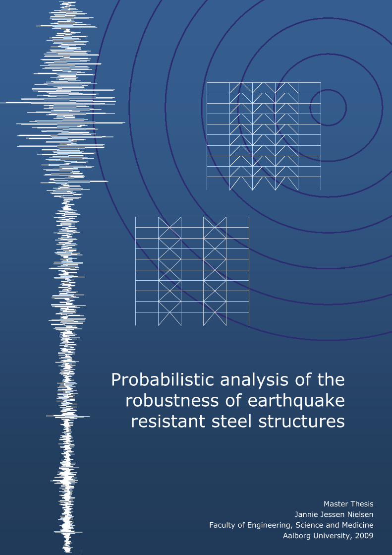
Probabilistic analysis of the robustness of earthquake resistant steel structures
Master Thesis
Jannie Jessen Nielsen
Faculty of Engineering, Science and Medicine
Aalborg University, 2009

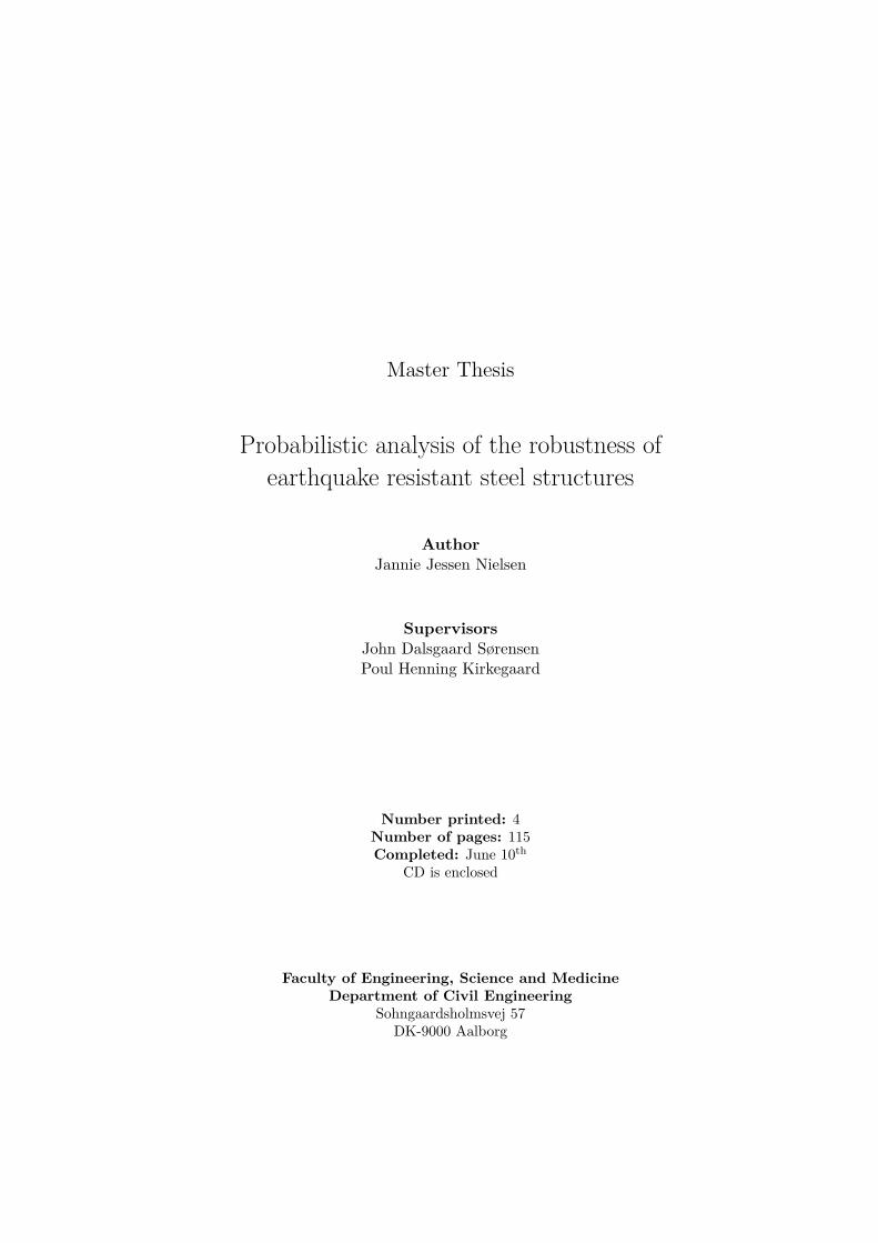
Master Thesis
Probabilistic analysis of the robustness ofearthquake resistant steel structures
AuthorJannie Jessen Nielsen
SupervisorsJohn Dalsgaard SørensenPoul Henning Kirkegaard
Number printed: 4Number of pages: 115Completed: June 10th
CD is enclosed
Faculty of Engineering, Science and MedicineDepartment of Civil Engineering
Sohngaardsholmsvej 57DK-9000 Aalborg

2
Preface
This master thesis serves as documentation of the authors Master of Sci-ence degree in Civil Engineering and it has been prepared at the Faculty ofEngineering, Science and Medicine at Aalborg University.
The title is Probabilistic analysis of the robustness of earthquake resistantsteel structures, and it is a short candidate project prepared in the periodFebruary 2nd – June 10th 2009. Basis knowledge about earthquake designwas gained during an internship at Ramboll Aalborg at the 3th semester ofthe candidate program, and additional knowledge has been gained throughliterature study.
A CD with MATLAB programs, finite element models and this thesis inpdf-format is enclosed.
Acknowledgements
The undersigned would like to acknowledge Ramboll Aalborg for putting acomputer with Robot [Robobat 2008] license for disposal.
June 10th 2009 Jannie Jessen Nielsen
3

4
Abstract
The aim of this project was to investigate whether structures designed forearthquake loads were robust too. Two steel structures with ten stories andfive bays in each direction and with eccentric and concentric braces in thefacades respectively have been analyzed using pushover analyzes. The per-formance for a given ground acceleration have been found using a responsespectrum reduced due to the ductile behavior found in the pushover analysiswith the method from ATC-40.
The robustness has been assessed using a deterministic, probabilistic andrisk based approach, where intact and damaged structures were analyzed. Inthe deterministic assessment the robustness was analyzed in relation to staticand seismic horizontal loads, and the influence of ductility and hardeningof the material was investigated. In the probabilistic assessment aleatoricand epistemic uncertainties were taken into account in the estimation of theannual probability of failure due to earthquakes, and two different robustnessindices were calculated, one based on the probability of failure and one basedon the reliability index. Finally a risk based approach was used where bothdirect and indirect consequences were taken into account.
The analyzes have shown that the damaged structures will often have a be-havior that is different from that of the original structure, because the yield-ing mechanisms does not work the way they are designed to when membersare missing. Thus the global ductile behavior for damaged structures wasfound to have great importance for the earthquake related robustness, andthe structural configuration was especially important for the performance.This means that structures designed for seismic actions will not necessarilybe robust towards seismic loads, as this depends on the structural configu-ration.
5

6

Resume
Formålet med dette projekt var at undersøge om konstruktioner dimen-sioneret for seismiske laster også er robuste. To stålkonstruktioner medhver ti etager og fem sektioner i hver retning og med hhv. excentriske ogkoncentriske afstivere er blevet analyseret vha. pushoveranalyser. Opførslenved en givet grundacceleration er beregnet vha. et responsspektrum reduc-eret afhængigt af duktiliteten fundet med pushoveranalysen med metodenfra ATC-40.
Robustheden er blevet vurderet med hhv. en deterministisk, probabilistiskog risikobaseret tilgang, hvor intakte og skadede konstruktioner blev analy-seret. Med den deterministiske tilgang blev robustheden analyseret i relationtil både statisk og seismisk horisontal last, og påvirkningen af duktilitet oghærdning af materialet blev undersøgt. Med den probabilistiske tilgang blevder taget hensyn til aleatoriske og epistemiske usikkerheder i beregningen afden årlige svigtsandsynlighed pga. jordskælv, og to forskellige robusthedsin-dekser blev beregnet, ét baseret på svigtsandsynligheden og ét baseret påsikkerhedsindekset. Endelig blev der brugt en risikobaseret tilgang, hvor derblev taget højde for både direkte og indirekte konsekvenser.
Analyserne viste, at skadede konstruktioner ofte vil have en opførsel som erforskellig fra den intakte konstruktion, idet de energidissiperende mekanis-mer ikke virker på den måde de er dimensioneret til, når nogle konstruktion-selementer mangler. Derfor havde den globale duktile opførsel af skadedekonstruktioner stor indflydelse på den jordskælvsrelaterede robusthed, ogden strukturelle konfiguration var særligt vigtig for opførslen. Dette bety-der, at konstruktioner der er dimensioneret for seismiske påvirkninger ikkenødvendigvis er robuste ift. seismiske laster, da det afhænger af den struk-turelle konfiguration.
7

8
Contents
1 Introduction 111.1 Performance based seismic design . . . . . . . . . . . . . . . . 11
1.1.1 Response of structures . . . . . . . . . . . . . . . . . . 121.2 Robustness . . . . . . . . . . . . . . . . . . . . . . . . . . . . 16
1.2.1 Strategies to ensure robustness . . . . . . . . . . . . . 181.2.2 Methods to assess robustness . . . . . . . . . . . . . . 21
1.3 Robustness in seismic design . . . . . . . . . . . . . . . . . . 241.4 Aim of the project . . . . . . . . . . . . . . . . . . . . . . . . 26
1.4.1 Methods . . . . . . . . . . . . . . . . . . . . . . . . . . 261.4.2 Contents . . . . . . . . . . . . . . . . . . . . . . . . . 26
2 Structural seismic analyzes 292.1 Structures . . . . . . . . . . . . . . . . . . . . . . . . . . . . . 29
2.1.1 Lateral load resisting systems . . . . . . . . . . . . . . 312.1.2 Seismic demands . . . . . . . . . . . . . . . . . . . . . 31
2.2 Nonlinear modeling of the structures . . . . . . . . . . . . . . 332.2.1 Structural systems . . . . . . . . . . . . . . . . . . . . 332.2.2 Nonlinear hinges . . . . . . . . . . . . . . . . . . . . . 342.2.3 Modeling of eccentrically braced frame . . . . . . . . . 352.2.4 Modeling of concentrically braced frame . . . . . . . . 39
2.3 Performance of structures . . . . . . . . . . . . . . . . . . . . 412.3.1 Eccentrically braced frame . . . . . . . . . . . . . . . . 412.3.2 Concentrically braced frame . . . . . . . . . . . . . . . 44
2.4 Summary . . . . . . . . . . . . . . . . . . . . . . . . . . . . . 47
3 Assessment of robustness 493.1 Structural configuration . . . . . . . . . . . . . . . . . . . . . 49
3.1.1 Redundancy and ductility . . . . . . . . . . . . . . . . 493.1.2 Isolation by compartmentalization . . . . . . . . . . . 503.1.3 Design of key elements . . . . . . . . . . . . . . . . . . 51
3.2 Behavior of damaged systems . . . . . . . . . . . . . . . . . . 513.2.1 Eccentrically braced frame . . . . . . . . . . . . . . . . 523.2.2 Concentrically braced frame . . . . . . . . . . . . . . . 55
3.3 Deterministic assessment of robustness . . . . . . . . . . . . . 56
9
10 CONTENTS
3.3.1 Load type . . . . . . . . . . . . . . . . . . . . . . . . . 563.3.2 Results . . . . . . . . . . . . . . . . . . . . . . . . . . 58
3.4 Other materials . . . . . . . . . . . . . . . . . . . . . . . . . . 643.4.1 Analyzes . . . . . . . . . . . . . . . . . . . . . . . . . 65
3.5 Summary . . . . . . . . . . . . . . . . . . . . . . . . . . . . . 69
4 Probabilistic seismic analysis 714.1 Uncertainties in seismic risk assessment . . . . . . . . . . . . 714.2 Procedure for seismic risk assessment . . . . . . . . . . . . . . 72
4.2.1 Capacity . . . . . . . . . . . . . . . . . . . . . . . . . 734.2.2 Demand . . . . . . . . . . . . . . . . . . . . . . . . . . 74
4.3 Probabilistic seismic analyzes of the structures . . . . . . . . 764.3.1 Capacity of the structure . . . . . . . . . . . . . . . . 764.3.2 Seismic demand . . . . . . . . . . . . . . . . . . . . . 764.3.3 Limit state probability . . . . . . . . . . . . . . . . . . 794.3.4 Sensitivity analysis . . . . . . . . . . . . . . . . . . . . 80
4.4 Probabilistic assessment of robustness . . . . . . . . . . . . . 824.4.1 Eccentrically braced frame . . . . . . . . . . . . . . . . 824.4.2 Concentrically braced frame . . . . . . . . . . . . . . . 83
4.5 Comparison . . . . . . . . . . . . . . . . . . . . . . . . . . . . 844.6 Summary . . . . . . . . . . . . . . . . . . . . . . . . . . . . . 86
5 Risk analysis 875.1 Analyzes . . . . . . . . . . . . . . . . . . . . . . . . . . . . . . 89
5.1.1 Robustness index . . . . . . . . . . . . . . . . . . . . . 925.2 Summary . . . . . . . . . . . . . . . . . . . . . . . . . . . . . 93
6 Summary 956.1 Conclusion . . . . . . . . . . . . . . . . . . . . . . . . . . . . 97
Bibliography 99
A Time history analysis in Robot 105A.1 Time history of linear SDOF system . . . . . . . . . . . . . . 105A.2 Time history of nonlinear SDOF system . . . . . . . . . . . . 108A.3 Conclusion on tests . . . . . . . . . . . . . . . . . . . . . . . . 108
B Nonlinear static performance based analysis 109B.1 Capacity curve . . . . . . . . . . . . . . . . . . . . . . . . . . 109B.2 Performance point . . . . . . . . . . . . . . . . . . . . . . . . 110
B.2.1 Hysteretic damping . . . . . . . . . . . . . . . . . . . 111
C Programs 115
Chapter 1
Introduction
During the last decade there has been increased focus on the subject robust-ness. This is caused by collapses such as Ronan Point (1968), World TradeCenter (2001), Siemens Arena in Ballerup (2003), and The Bad ReichenhallIce-Arena Collapse (2006). In Eurocode 0 the following robustness require-ment can be found: ”A structure shall be designed and executed in such away that it will not be damaged by events such as: explosion, impact, andthe consequences of human errors, to an extent disproportionate to the orig-inal cause.”[EN 1990:2002 2002]. Lots of research has been done within thearea, and different definitions and methods to assess robustness have beenproposed (eg [Starossek & Wolff 2005] [Canasius, Sørensen & Baker 2007][Baker, Schubert & Faber 2008]). In this project the robustness of structuresdesigned for seismic loads is considered when the structures are exposed toseismic loads. This chapter introduces the two main topics for the project,seismic design and robustness.
1.1 Performance based seismic design
The load from an earthquake is an inertia load, caused by the accelerationsof the masses in the structure. Due to the equal displacement theory pro-posed by [Newmark & Hall 1982] the displacements of a yielding structurewill be the same as those of an elastic structure. When a structure yieldsduring an earthquake energy is dissipated in the yielding regions by hys-teresis processes, and the accelerations of the structure and thus the inertialload will be decreased compared to an elastic structure. The term seismicdemand is often used for an earthquake load.
Modern seismic codes use the concept of performance based design, where
11
12 CHAPTER 1. INTRODUCTION
different allowable damage levels (limit states) are set for different returnperiods of the earthquakes, with the objective to control the loss due toearthquakes [Bommer & Pinho 2006]. The damage of the structure is foundto be related to the maximum inter-story drift angle (ISDA) during an earth-quake [Ellingwood 2001]. Therefore the starting point for performance basedseismic design is the allowable ISDA, even though most present codes useforce based methods of analysis [Bazeos 2009].
The limit states can be defined as: [Ellingwood & Kinali 2009]
• Immediate Occupancy (IO):Onset of inelastic behavior
• Structural Damage (SD):Global lateral stiffness drops to half of initial value
• Collapse Prevention (CP):Onset of instability
For each limit state the corresponding ISDA can be found for a given struc-ture.
The design criteria for a seismic limit state is that the capacity has to exceedthe seismic demand. The capacity is a property of the structure, whereas thedemand is a property of the earthquake, but is changed due to the ductilityof the structure. There exist several different methods to design earthquakeresistant structures, and in the following some of the methods are outlined.
1.1.1 Response of structures
The dynamic response of a structure is dependent on the mass, stiffness,damping and load. For a viscously damped multi degree of freedom (MDOF)system the governing equation is:
Mx(t) + Cx(t) + K(x)x(t) = F(t) (1.1)
where M is the mass matrix, C is the damping matrix, K is the stiffnessmatrix, x is the node displacement vector, and F is the load vector. For anearthquake load F is time dependent, and if the analysis is nonlinear, K isdependent on x.
The performance of a structure is best evaluated using nonlinear meth-ods. The most precise analysis can be utilized with nonlinear time historyanalyzes of a spatial model with several bidirectional earthquake records
1.1. PERFORMANCE BASED SEISMIC DESIGN 13
as input motions. This analysis precisely takes the ductility into account,and it tells where the structure is damaged, thus it gives a good estimateof the performance of the entire structure during an earthquake. [Wen &Song 2003]
Response spectrum analysis
The nonlinear time history analysis has the disadvantage that various timeconsuming analyzes has to be run in order to use this design method. Amuch faster analysis can be performed, if a linear analysis is made, andthe nonlinearity is taken into account by reducing the seismic demand witha behavior factor. Instead of making a time history analysis, the MDOFsystem can be decoupled to a number of single degree of freedom (SDOF)systems, and a response spectrum can be used.
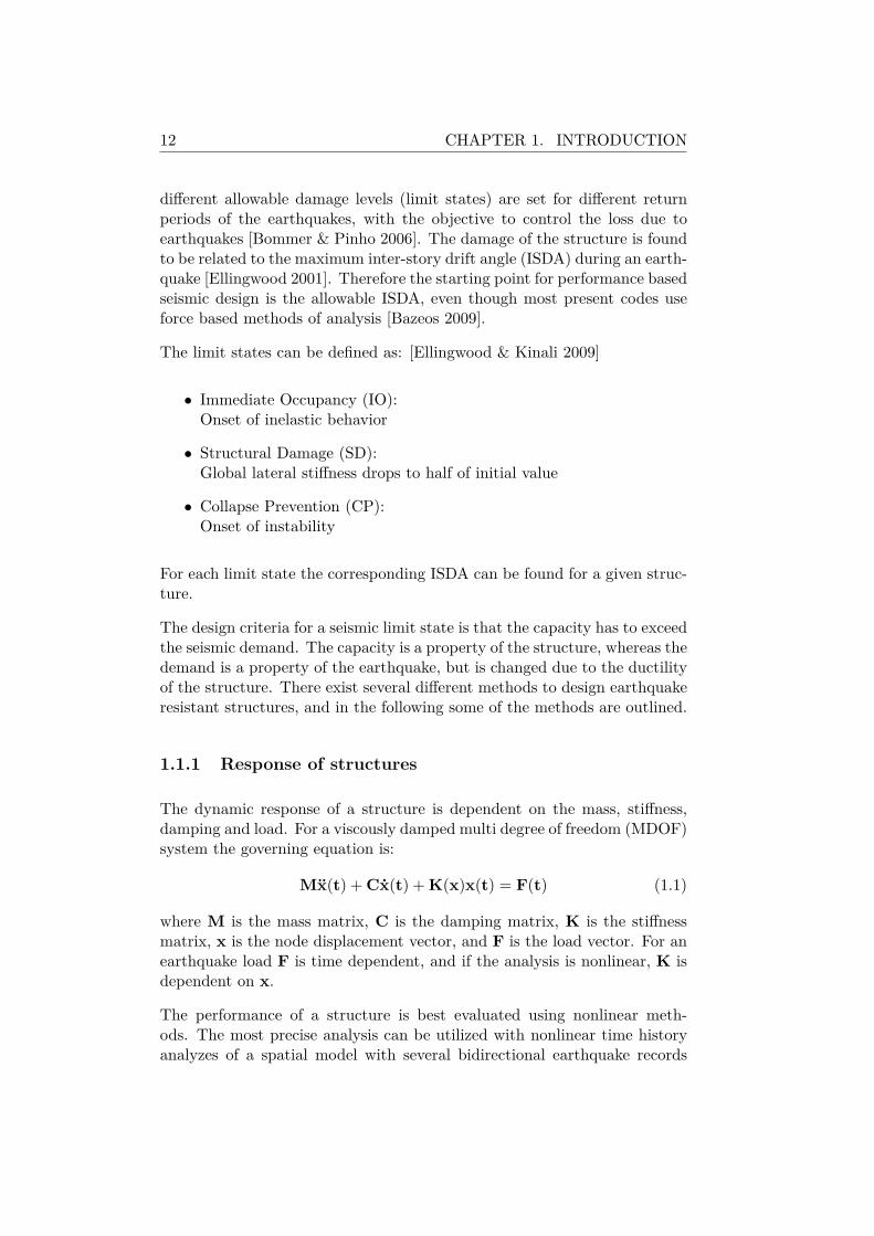
A response spectrum uses that for a linear SDOF system the peak responseacceleration to a given time history of an earthquake load can be found tobe dependent on the natural period of vibrations of the system. If there isa large amount of energy in the time history near the natural period of thestructure, the response is large. A response spectrum takes advantage of thisas it gives the peak spectral acceleration as function of the natural periodof vibrations of the structure for a specific damping level. The process ofmaking a response spectrum from a specific time history is shown in figure1.1.
For an elastic MDOF system a modal analysis can be utilized, which re-sults in the natural vibration periods, mode shapes, and mass participationpercentages for the structure. For each natural period the peak spectral ac-celeration, reduced due to the ductility, is found and applied to the massescorresponding to the the mode shapes and mass participation percentages.At last the total response is found by combining the responses of each mode.Many codes eg [EN 1998-1:2004 2004] allows the use of this method forearthquake analyzes.
The main flaw of this method is related to the way, ductility is taken intoaccount. The reduction factor is set due to the type of structural system,the deformations are calculated with large uncertainty, and the analysis tellsnoting about the size and location of the structural damage. This can bedone with the static pushover analysis that has become a frequently usedtool for seismic design [Poursha, Khoshnoudian & Moghadam 2009].
14 CHAPTER 1. INTRODUCTION
a
k2
k1
k3
k4
T1 T2 T3 T4 T
Sp
ectr
al
Accele
rati
on
[m
/s
2]
a
a
t
t
t
t
Structural
response
T2
T1
T3
T4
Input
Input
Input
Input
SDOF
systems
a
t
Earthquake
time series
m2
m1
m3
m4
a
Figure 1.1: Calculation of a response spectrum based on an earthquake acceleration timeseries. This is used as input for SDOF systems with different natural vibration periods,and a time series of the structural response is calculated for each SDOF system. Themaximum response is determined for each, and the values are plotted as function of thenatural vibration periods.
1.1. PERFORMANCE BASED SEISMIC DESIGN 15
Pushover analysis
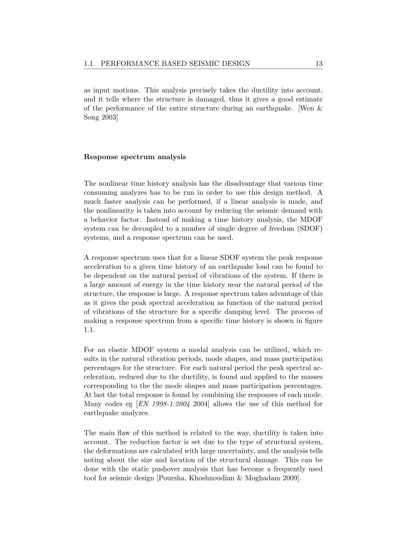
The pushover analysis is a static nonlinear analysis, where the post yieldbehavior of the structure is investigated. A lateral force, distributed due tothe masses and the mode shape with largest mass participation, is appliedand increased until collapse is reached. The corresponding deformations arefound for each load step. The total lateral force is plotted as function of theroof displacement to form the capacity curve, as shown in figure 1.2.
Figure 1.2: Use of pushover analysis to make the capacity curve.
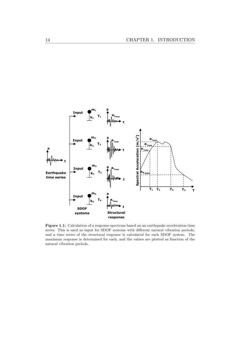
This curve can be converted to a capacity spectrum corresponding to aSDOF system where the spectral acceleration is plotted as function of thespectral displacement. The seismic demand is controlled by the elastic re-sponse spectrum that can be plotted in this diagram as well, as shown infigure 1.3.
Figure 1.3: Capacity spectrum and elastic demand spectrum.
Due to the hysteretic damping, estimated on basis of the shape of the ca-pacity spectrum, the elastic response spectrum is reduced. The intersectionbetween the reduced response spectrum and the capacity spectrum is theperformance point, and gives an estimate on the displacement and the dam-age of the structure for a given elastic response spectrum. The method is
16 CHAPTER 1. INTRODUCTION
explained further in appendix B.
This method is limited to structures where only one mode shape contributessignificantly to the response, but several extended methods have been pro-posed, where more modes are taken into account [Poursha et al. 2009].
1.2 Robustness
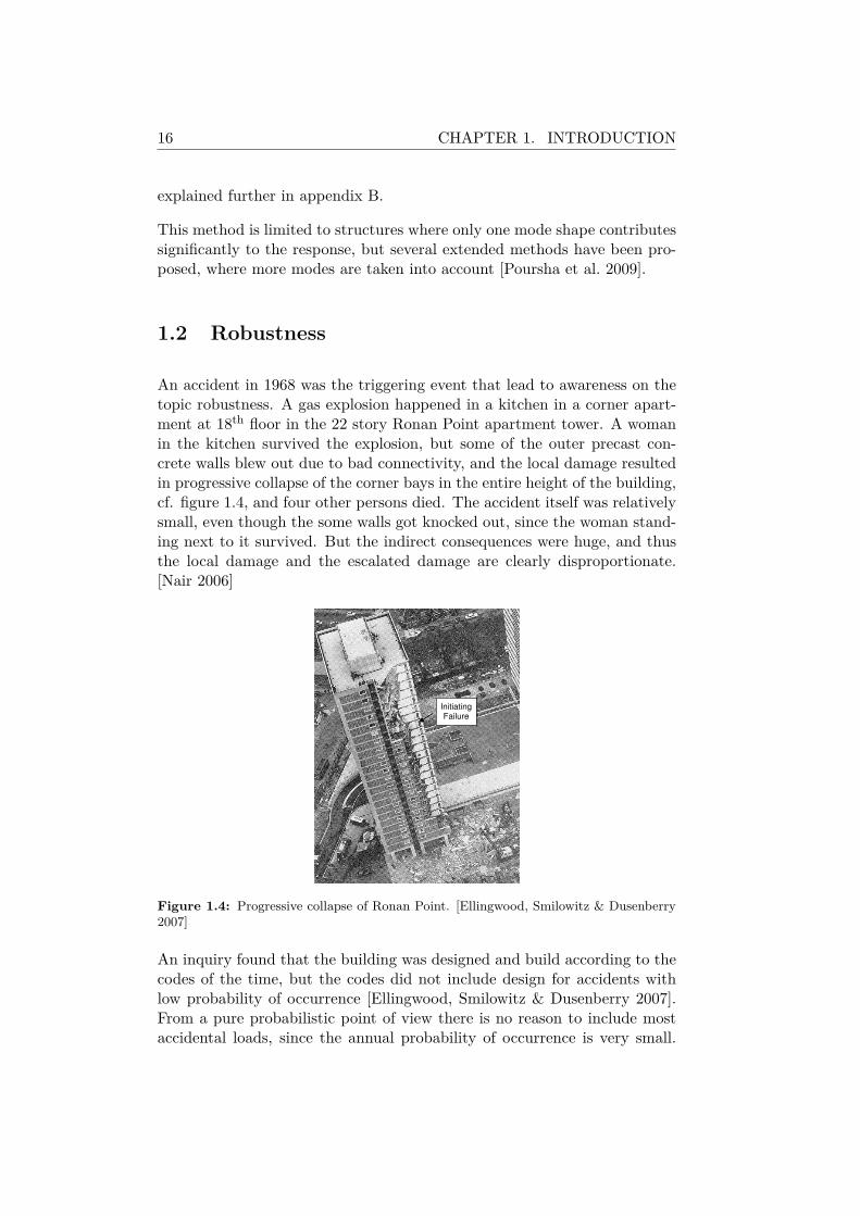
An accident in 1968 was the triggering event that lead to awareness on thetopic robustness. A gas explosion happened in a kitchen in a corner apart-ment at 18th floor in the 22 story Ronan Point apartment tower. A womanin the kitchen survived the explosion, but some of the outer precast con-crete walls blew out due to bad connectivity, and the local damage resultedin progressive collapse of the corner bays in the entire height of the building,cf. figure 1.4, and four other persons died. The accident itself was relativelysmall, even though the some walls got knocked out, since the woman stand-ing next to it survived. But the indirect consequences were huge, and thusthe local damage and the escalated damage are clearly disproportionate.[Nair 2006]
InitiatingFailure
Figure 1.4: Progressive collapse of Ronan Point. [Ellingwood, Smilowitz & Dusenberry2007]
An inquiry found that the building was designed and build according to thecodes of the time, but the codes did not include design for accidents withlow probability of occurrence [Ellingwood, Smilowitz & Dusenberry 2007].From a pure probabilistic point of view there is no reason to include mostaccidental loads, since the annual probability of occurrence is very small.
1.2. ROBUSTNESS 17
The consequences, however, can be very huge if an accident happens anyway.This can be included in the design by examining the risk, R, defined basicallyas:
R = PfC (1.2)
where Pf is the probability of failure and C are the consequences with anappropriate measure.
Another flaw of the design procedures in the building codes is that thesafety of structures is examined on element level instead of system level,thus the total safety of the structure is not directly investigated. If moreelements work together in a series system, the safety of the building can besignificantly less than the safety for each element. [Starossek & Wolff 2005]
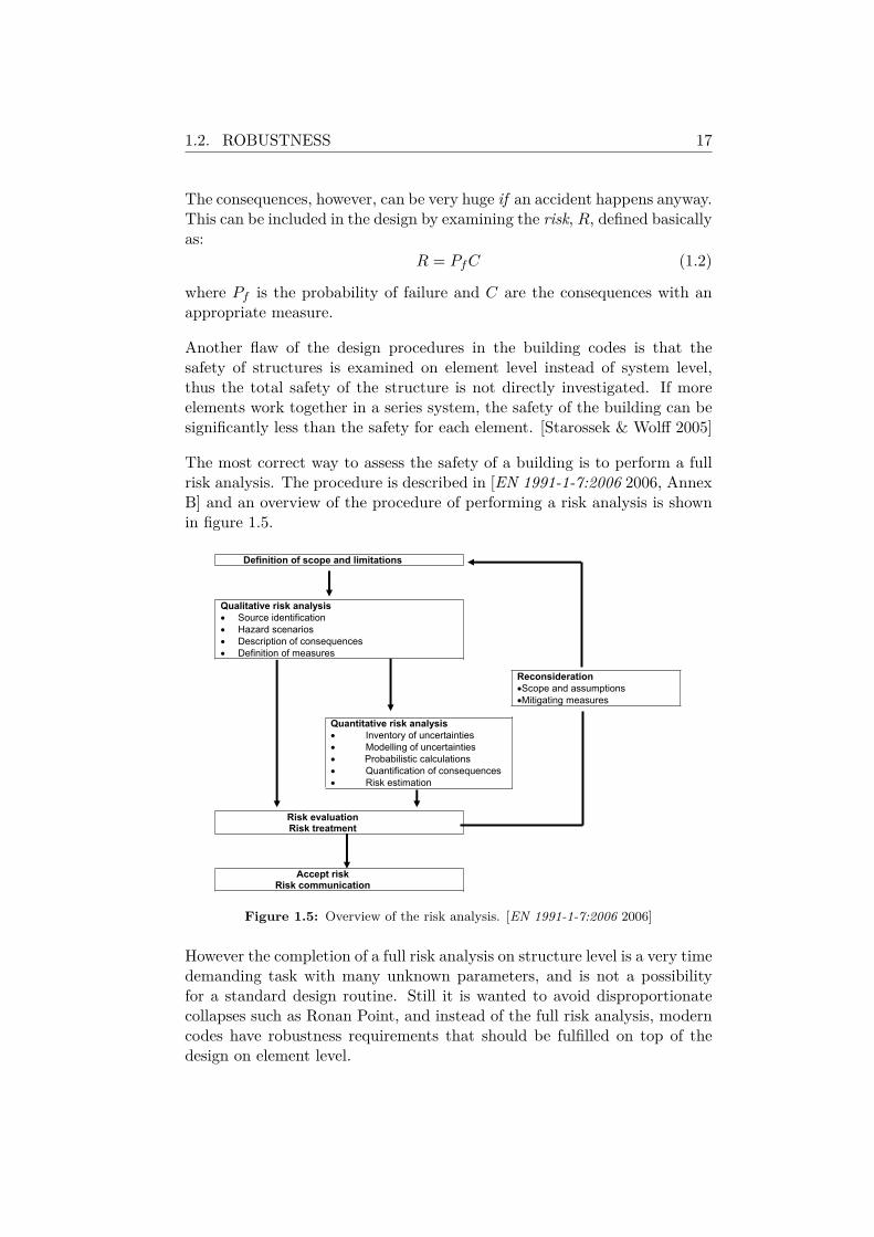
The most correct way to assess the safety of a building is to perform a fullrisk analysis. The procedure is described in [EN 1991-1-7:2006 2006, AnnexB] and an overview of the procedure of performing a risk analysis is shownin figure 1.5.
Definition of scope and limitations
Qualitative risk analysis
Source identification
Hazard scenarios
Description of consequences
Definition of measures
Reconsideration
Scope and assumptions
Mitigating measures
Quantitative risk analysis
Inventory of uncertainties
Modelling of uncertainties
Probabilistic calculations
Quantification of consequences
Risk estimation
Risk evaluation Risk treatment
Accept risk Risk communication
Figure 1.5: Overview of the risk analysis. [EN 1991-1-7:2006 2006]
However the completion of a full risk analysis on structure level is a very timedemanding task with many unknown parameters, and is not a possibilityfor a standard design routine. Still it is wanted to avoid disproportionatecollapses such as Ronan Point, and instead of the full risk analysis, moderncodes have robustness requirements that should be fulfilled on top of thedesign on element level.
18 CHAPTER 1. INTRODUCTION
1.2.1 Strategies to ensure robustness
In the Eurocodes such robustness requirements can be found in two docu-ments, [EN 1990:2002 2002] and [EN 1991-1-7:2006 2006]. The first requiresthat ”A structure shall be designed and executed in such a way that it willnot be damaged by events such as: explosion, impact, and the consequencesof human errors, to an extent disproportionate to the original cause.”[EN1990:2002 2002].
Robustness is meant to avoid failures caused by:
• Errors in the design
• Error during construction
• Lack of maintenance
• Unforeseeable events
The first three are most often caused by human errors, whereas the lastpoint is accidental loads. [Munch-Andersen 2009]
Accidental loads
In [EN 1991-1-7:2006 2006] different strategies for designing for accidentaldesign situations are listed.
In general there are strategies within two categories, design for identifiedactions and limiting extent of local damage. For identified accidents thestrategies fall into three categories:
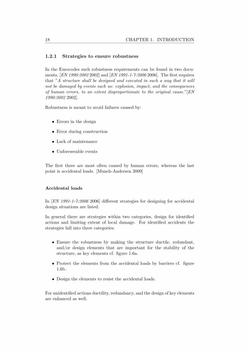
• Ensure the robustness by making the structure ductile, redundant,and/or design elements that are important for the stability of thestructure, as key elements cf. figure 1.6a.
• Protect the elements from the accidental loads by barriers cf. figure1.6b.
• Design the elements to resist the accidental loads.
For unidentified actions ductility, redundancy, and the design of key elementsare enhanced as well.
1.2. ROBUSTNESS 19
(a) Specific local resistance. (b) Protective barriers.
Figure 1.6: Strategies to survive accidental loads. [Starossek & Wolff 2005]
Loss of structural element scenario
These demands can also be found in the NIST document Best Practise forReducing the Potential for Progressive Collapse in Buildings [Ellingwood,Celik & Kinali 2007]. To avoid progressive collapses in an event with a lossof a structural element the structure should have the following properties:(cite from [Vrouwenvelder & Sørensen 2009])
Redundancy: Incorporation of redundant load paths in the vertical loadcarrying system.
Ties: Using an integrated system of ties in three directions along the prin-cipal lines of structural framing.
Ductility: Structural members and member connections have to maintaintheir strength through large deformations (deflections and rotations)so the load redistribution(s) may take place.
Adequate shear strength: As shear is considered as a brittle failure, struc-tural elements in vulnerable locations should be designed to withstandshear load in excess of that associated with the ultimate bending mo-ment in the event of loss of an element.
Capacity for resisting load reversals: The primary structural elements(columns, girders, roof beams, and lateral load resisting system) andsecondary structural elements (floor beams and slabs) should be de-signed to resist reversals in load direction at vulnerable locations.
Connections (connection strength): Connections should be designed insuch way that it will allow uniform and smooth load redistributionduring local collapse.
Key elements: Exterior columns and walls should be capable of spanningtwo or more stories without bucking, columns should be designed towithstand blast pressure etc.
20 CHAPTER 1. INTRODUCTION
Alternate load path(s): After the basic design of structure is done, a re-view of the strength and ductility of key structural elements is requiredto determine whether the structure is able to ”bridge” over the initialdamage.
Key elements are elements that are important for the overall stability of thestructure, and thereby corresponds to elements in a series system. Accordingto the Danish National Annex for Eurocode 0, [EN 1990 DK NA:2007 2007],the partial factor on key elements should be increased with a factor 1.2. Thisvalue corresponds to the factor the strength of elements in a series systemshould be increased, to obtain the same safety as equivalent elements in aparallel system [Sørensen & Christensen 2006].
In many cases, however, it is better to ensure the robustness by choosinga redundant structure. A redundant structure is characterized by beingstatically indeterminate. Like a parallel system the structure is able toprovide alternate load paths, if the structure is damaged. Ductility is aproperty of the material to allow large strains. In general a ductile structureis more redundant than a brittle, as the elements retain its strength at largestrains, at thereby allows the structure to activate the alternate load paths.
Isolation by compartmentalization
Another strategy to prevent progressive collapse is isolation by compart-mentalization. Here the idea is to allow local damage to happen with thepurpose that the remaining structure is not overloaded.
The Bad Reichenhall Ice-Arena collapse in 2006 is an example where thisstrategy might have helped. The collapse happened a winter day, where theroof was covered by snow. The load caused a timber beam to collapse, andas the purlins where strong and stiff, a progressive collapse caused the entireroof to collapse. An investigation found that the snow load did not exceedthe design load, but design errors and unforeseen degradation of the strengthof the glue due to the use of a new technology, had caused the beams to besignificantly weaker that expected. The redundancy of the structure was thereason that the design errors caused a total collapse and not just a limitedcollapse. [Dietsch 2009]
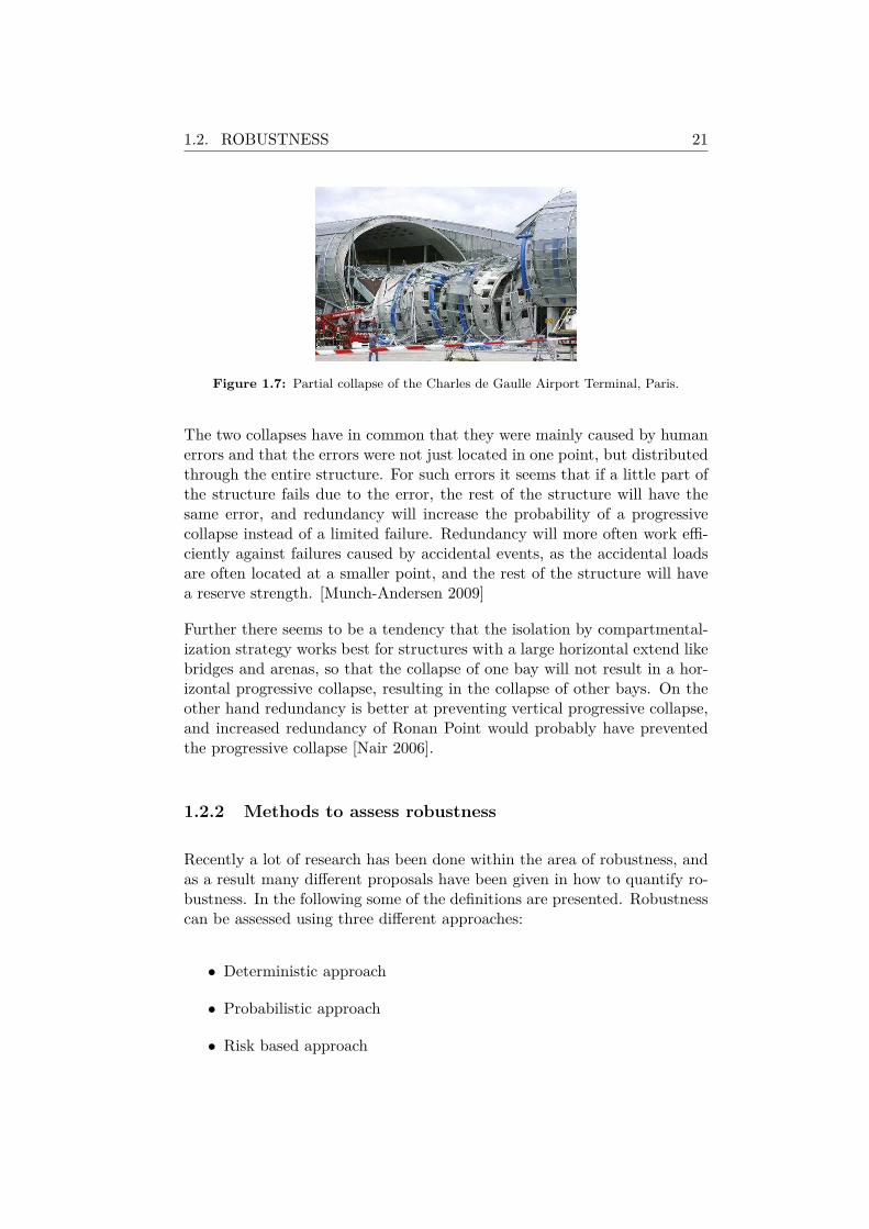
In the case of the partial collapse of the Charles de Gaulle Airport Terminalin 2004, there were limited interconnections between the bays, and only onebay collapsed cf. figure 1.7. The collapse was caused by poor workman-ship and design errors, and increased redundancy might have resulted in aprogressive collapse of more bays. [Starossek & Wolff 2005]
1.2. ROBUSTNESS 21
Figure 1.7: Partial collapse of the Charles de Gaulle Airport Terminal, Paris.
The two collapses have in common that they were mainly caused by humanerrors and that the errors were not just located in one point, but distributedthrough the entire structure. For such errors it seems that if a little part ofthe structure fails due to the error, the rest of the structure will have thesame error, and redundancy will increase the probability of a progressivecollapse instead of a limited failure. Redundancy will more often work effi-ciently against failures caused by accidental events, as the accidental loadsare often located at a smaller point, and the rest of the structure will havea reserve strength. [Munch-Andersen 2009]
Further there seems to be a tendency that the isolation by compartmental-ization strategy works best for structures with a large horizontal extend likebridges and arenas, so that the collapse of one bay will not result in a hor-izontal progressive collapse, resulting in the collapse of other bays. On theother hand redundancy is better at preventing vertical progressive collapse,and increased redundancy of Ronan Point would probably have preventedthe progressive collapse [Nair 2006].
1.2.2 Methods to assess robustness
Recently a lot of research has been done within the area of robustness, andas a result many different proposals have been given in how to quantify ro-bustness. In the following some of the definitions are presented. Robustnesscan be assessed using three different approaches:
• Deterministic approach
• Probabilistic approach
• Risk based approach
22 CHAPTER 1. INTRODUCTION
Deterministic
For offshore structures a robustness measure can be obtained using the re-serve strength ratio (RSR) defined as:
RSR = RCSC
(1.3)
where RC is the base shear capacity and SC is the design load. [Straub &Faber 2005]
The redundancy (robustness) can be evaluated using the residual influencefactor (RIF ):
RIFi = RSRFiRSRintact
(1.4)
Where RSRintact and RSRFi is the reserve strength ratio for an intact struc-ture and a structure where element i is damaged respectively.
If the design load is equal for the intact and damaged structure, the RIFcan be rewritten to:
RIFi =RC(Fi)RC(intact)
(1.5)
Thus the redundancy can be evaluated as the fraction between the capacityof the damaged and the intact structure. If the intact and damaged struc-tures have same capacity the value is one, if the damaged structure has nocapacity it is zero.
For a lateral load the base shear capacities can be found by performing astatic pushover analysis.
Probabilistic
In a probabilistic formulation the total probability of collapse P (C) can bewritten as:
P (C) =∑
i
∑
j
P (C|Ei ∩Dj)P (Dj |Ei)P (Ei) (1.6)
where Ei is the i’th exposure and Dj is the j’th damage type, P (Ei) is theprobability of the exposure, P (Dj |Ei) is the probability of damage given theexposure, and P (C|Ei∩Dj) is the probability of collapse given the exposureand damage. Thus the robustness can be increased by decreasing one of thefactors. [Sørensen & Christensen 2006]
For unidentified accidental loads the probability of the exposure, P (Ei), isin general very small and can be very hard to assess, and the probability
1.2. ROBUSTNESS 23
of damage given the exposure, P (Dj |Ei), is hard to assess too. Regardlessof the accidental load the robustness can then be increased by decreasingthe probability of collapse given the exposure and damage, P (C|Ei ∩ Dj).This corresponds to investigating the ability of the structure to resist loadin a damaged state using the the alternate load path method. [Ellingwood,Smilowitz & Dusenberry 2007]
A probabilistic redundancy index, βR, was proposed by [Frangopol & Curley1987]:
βR = βintactβintact − βdamaged (1.7)
where βintact is the reliability index of the intact structure and βdamagedis the reliability index of the damaged structure. If the reliability index isunchanged for the damaged structure it is infinite, and if there is no capacityof the damaged structure it is one.
The probability of failure and the reliability index is related through thefollowing expression:
P (C) = Φ(−β) (1.8)
A vulnerability index was proposed by [Lind 1995] as:
V = P (Rd,S)P (R0,S) (1.9)
where P (Rd,S) is the probability of failure for a damaged structure, andP (R0,S) is the probability of failure for the intact structure. The reciprocalof this is the damage tolerance factor:
Td = P (R0,S)P (Rd,S) (1.10)
which is also a measure of the robustness of the structure. This measureis one if the failure probability is equal for the damaged and undamagedstructure, and zero if the failure probability of the damaged structure isinfinite. Hereby this measure can be compared with the deterministic RIFvalue.
Risk analysis
A risk analysis is the most complete way to assess the safety of a structure.In a risk analysis there are three influencing factors; hazard, consequencesand context. The hazard could be an earthquake, the consequences couldbe economic losses and losses of lives caused by a collapse. The context
24 CHAPTER 1. INTRODUCTION
is important too, as individuals and eg a government have different viewsupon acceptable risk. Acceptable risk in structural engineering is a relativeterm, and must be calibrated against other risks in the society. Further thecost for decreasing the risk, or gain for increasing the risk will influence thechoice. The acceptable risk is orders of magnitude larger for risks taken vol-untary than those taken by society. Risk can be measured in different terms,and in building codes the main objective is to protect human lives and tominimize considerable societal consequences (economic and environmental).[Ellingwood, Smilowitz & Dusenberry 2007]
The total risk can be found as:
R = Rdir +Rindir =∑
i
∑
j
Cdir,ijP (Dj |Ei)P (Ei)+∑
i
∑
j
∑
k
Cindir,ijkP (Sk|Dj)P (Dj |Ei)P (Ei)
(1.11)
where Cdir,ij consequence of damage Dj due to exposure Ei and Cindir,ijk isthe consequence of comprehensive damages Sk given local damage Dj dueto exposure Ei [Vrouwenvelder & Sørensen 2009].
One way to increase the robustness is to minimize the indirect risk, givenby the second term in equation 1.11. With that in mind the risk basedrobustness index was proposed by [Baker et al. 2008]:
IRob = RdirRdir +Rindir
(1.12)
where Rdir is the direct risk associated to local damage, and Rindir is indirectrisk associated to comprehensive damage. It is one for a robust structurewith no indirect risk and zero for a structure that is not robust at all.
However, the risk can also be reduced by reducing the first term in equation1.11, and this means that the risk based robustness index will not always beconsistent with a full risk analysis. [Vrouwenvelder & Sørensen 2009]
1.3 Robustness in seismic design
As the previous sections might have illustrated, seismic resistant structuresare in general born with some attributes that ensures some robustness of thestructures. This is due to requirements in seismic codes and the methodsused for the seismic design.
The influence of different factors, normally considered as contributing tothe redundancy of structures was investigated by [Wen & Song 2003]. They
1.3. ROBUSTNESS IN SEISMIC DESIGN 25
evaluated the factors by calculating the column drift ratio for different lat-eral systems using nonlinear time history analyzes with earthquake recordsas input. Because of the large uncertainty in seismic excitation and struc-tural resistance the redundancy was measured in terms of the probabilityof exceeding a limit state measured in terms of story drift. They foundthat the structural configuration was very important for the redundancy,and that the number of shear walls did not have a great importance for theredundancy, thus it is not crucial for the seismic behavior how many timesindeterminate a structure is.
The resistance against progressive collapse for seismically designed bracedsteel frames was investigated by [Khandelwal, El-Tawil & Sadek 2009]. Thedynamic response was found when columns and adjoining braces were in-stantaneously removed. The brace system, able to resist seismic loads, wasalso found to be capable of preventing progressive collapse. Only the non-braced corner columns were sensitive, thus the structural configuration wasfound very important for the progressive collapse resistance.
In general seismic resistant structures are designed to act inelastic duringsevere earthquakes, which requires that the proportion between columnsand beams is set due to the concept of capacity design. For a momentresistant structure this is ensured by the concept of strong column/weakbeam, meaning that plastic hinges will be developed in the beams and not inthe columns, so that many hinges have to be developed before the structurefails. Thus the structure is designed to fail in less fatal failure modes first,what gives an increase in the redundancy.
It is also a demand that the materials in a seismic resistant structure actductile, so that the structure retains its strength at large deformation, elsethe structure cannot benefit from the formation of the hinges. This was alsopointed out by [Bertero & Bertero 1999] as redundancy cannot be quantifiedalone in terms of over strength, since it is highly important that sufficientrotation capacity is available. This is an important feature for a redundantstructure, but the demands are even more crucial for a seismic resistantstructure. Not only shall it provide ductile behavior against a static load,but it also has to be able to survive hysteretic cycles in and out the plasticarea without loosing its strength. This sets requirements for the connectionsand for use of stiffeners, so that buckling of the web will not prevent thecycles.
26 CHAPTER 1. INTRODUCTION
1.4 Aim of the project
Since seismic resistant structures are in general ductile and redundant, onemight assume that they are also robust. The aim of this project is to analyzethe robustness of seismically designed steel structures, and thereby seek toinvestigate it. The robustness will be quantified through different measures,and in addition the influence of the ductility of the material is investigated.
The analyzes of the robustness will be performed in connection with seismicloads. The studied case is seismic resistant steel structures that are damagedeg by an impact or because of design or execution errors. It is investigatedhow these damaged structures will perform during an earthquake comparedto the intact structure. The behavior towards vertical loads is not includedin the analysis.
1.4.1 Methods
The seismic behavior is best evaluated using time history analyzes withbidirectional earthquake records as input for inelastic spatial models [Wen& Song 2003]. It has been chosen to use the finite element program Robotby Robobat [Robobat 2008] for the structural analyzes in this project. Sim-ple analyzes have been made in Robot to investigate, whether the build inopportunity to make time history analyzes could be used to make nonlinearanalyzes where the supports were subjected to an acceleration time history.As explained in appendix A this could not be done with reliable results, andthe options were to find another program or to make simpler analyzes. Thelatter was chosen because of limited time.
Instead nonlinear static pushover analyzes are used. To minimize the timeconsumption the analyzes are performed for plane structures, and thus thespatial effects are not taken into account.
The robustness is evaluated using a deterministic, probabilistic, and riskbased approach. For the probabilistic analyzes first order reliability methods(FORM) are used.
1.4.2 Contents
Two seismically designed braced steel structures are chosen for case studiesfor this project. At first the nonlinear modeling of the structures is evalu-ated, and the seismic behavior is analyzed for both structures.

1.4. AIM OF THE PROJECT 27
The overall robustness of the structures is discussed, and it is assessed forhorizontal loads only, both for seismic loads and static loads. It is assessedusing deterministic, probabilistic and risk based approaches. The robustnessis evaluated on basis of the difference between the intact structure and adamaged structure. For the analysis of the damaged structure a limitedpart of the structure is removed, that is, a column and adjoining braces.
Further the influence of the material is investigated by making similar ana-lyzes for structures where the ductility and hardening is changed.

28 CHAPTER 1. INTRODUCTION
Chapter 2
Structural seismic analyzes
In this chapter the seismic behavior of two steel structures are investigated.
2.1 Structures
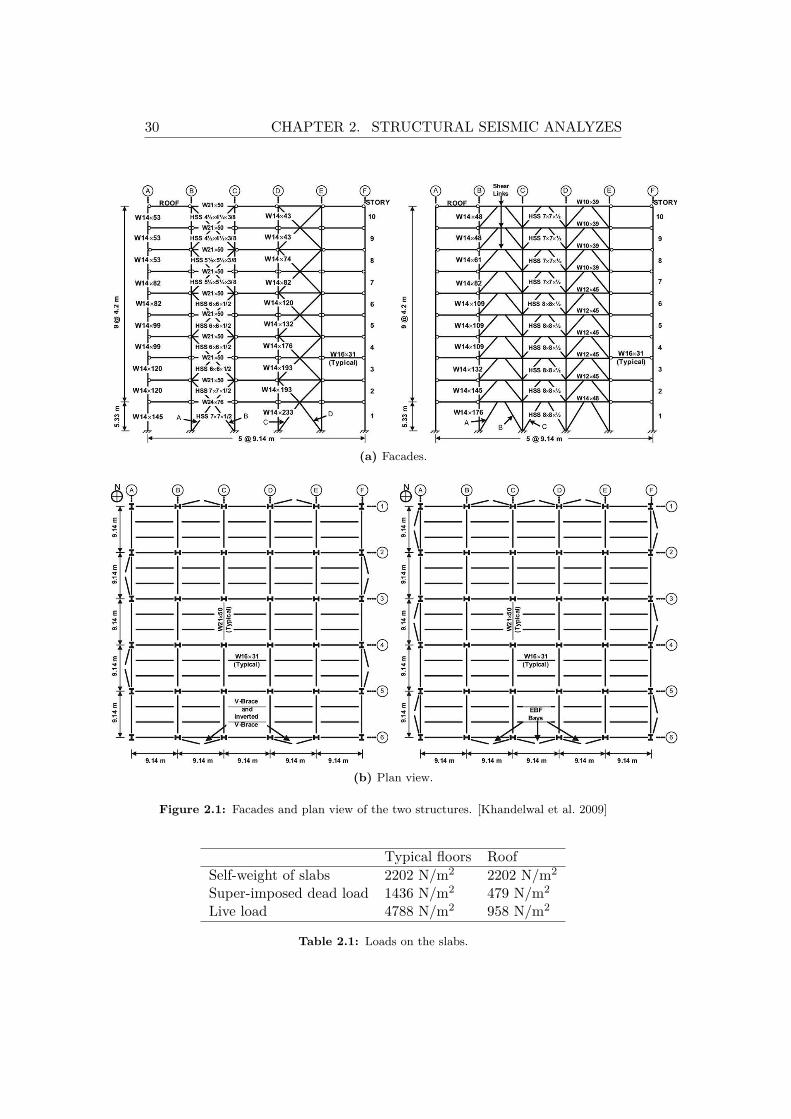
The prototype structures chosen for this analysis were originally design byThe National Institute of Standards and Technology (NIST), and have beenused for progressive collapse studies by [Khandelwal et al. 2009]. Both struc-tures have ten stories and five bays in each direction. They are steel struc-tures with a lateral load resisting system consisting of braced frames in thefacades and concrete slaps are distributing the loads to the facades.
The structures are designed for seismic actions corresponding to Seattle,Washington with high seismic activety and Atlanta, Georgia with less seis-mic activity respectively. The structure designed for high seismic activityis an eccentrically braced frame (EBF), whereas the other is a special con-centrically braced frame (SCBF), and both structures can be seen in figure2.1.
All sections are taken from the American AISC Shapes Database. Thebraces are made of Hollow Steel Sections (HSS), and the other members areI-sections from the W-series. A500-46 steel (Fy = 317 MPa) is used for thebraces and A992-50 (Fy = 345 MPa) is used for the other sections.
The loads on the slabs are listed in table 2.1. The live load is reduced basedon [ASCE 7-05 2005, Sec. 4.8.1]. Each facade gets the seismic load fromhalf of the building.
29
30 CHAPTER 2. STRUCTURAL SEISMIC ANALYZES
(a) Facades.
(b) Plan view.
Figure 2.1: Facades and plan view of the two structures. [Khandelwal et al. 2009]
Typical floors RoofSelf-weight of slabs 2202 N/m2 2202 N/m2
Super-imposed dead load 1436 N/m2 479 N/m2
Live load 4788 N/m2 958 N/m2
Table 2.1: Loads on the slabs.
2.1. STRUCTURES 31
2.1.1 Lateral load resisting systems
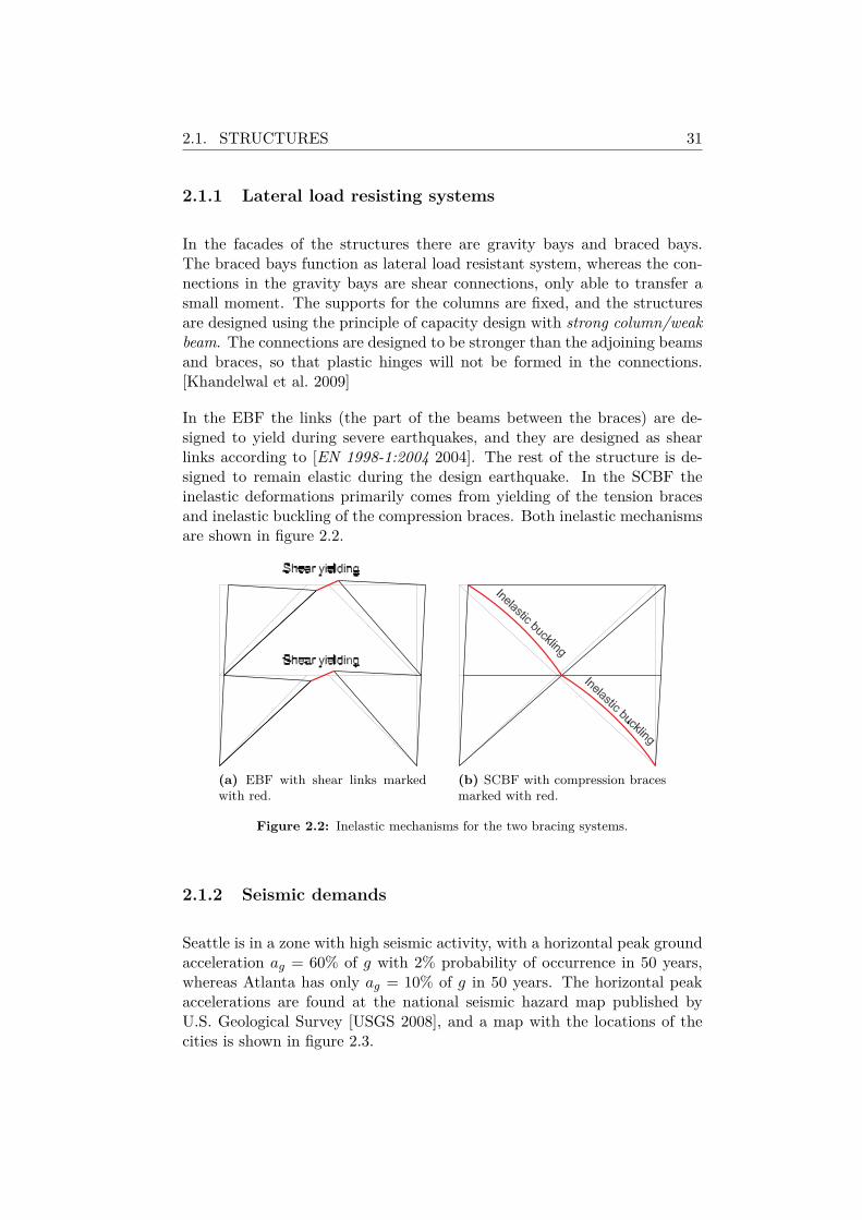
In the facades of the structures there are gravity bays and braced bays.The braced bays function as lateral load resistant system, whereas the con-nections in the gravity bays are shear connections, only able to transfer asmall moment. The supports for the columns are fixed, and the structuresare designed using the principle of capacity design with strong column/weakbeam. The connections are designed to be stronger than the adjoining beamsand braces, so that plastic hinges will not be formed in the connections.[Khandelwal et al. 2009]
In the EBF the links (the part of the beams between the braces) are de-signed to yield during severe earthquakes, and they are designed as shearlinks according to [EN 1998-1:2004 2004]. The rest of the structure is de-signed to remain elastic during the design earthquake. In the SCBF theinelastic deformations primarily comes from yielding of the tension bracesand inelastic buckling of the compression braces. Both inelastic mechanismsare shown in figure 2.2.
(a) EBF with shear links markedwith red.
(b) SCBF with compression bracesmarked with red.
Figure 2.2: Inelastic mechanisms for the two bracing systems.
2.1.2 Seismic demands
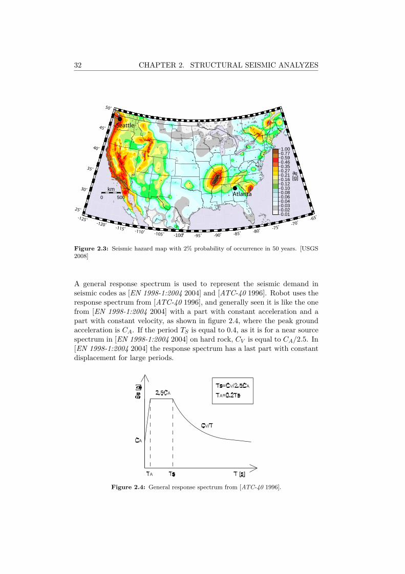
Seattle is in a zone with high seismic activity, with a horizontal peak groundacceleration ag = 60% of g with 2% probability of occurrence in 50 years,whereas Atlanta has only ag = 10% of g in 50 years. The horizontal peakaccelerations are found at the national seismic hazard map published byU.S. Geological Survey [USGS 2008], and a map with the locations of thecities is shown in figure 2.3.
32 CHAPTER 2. STRUCTURAL SEISMIC ANALYZES
-100
0 500
km
0.010.020.030.040.060.080.100.120.160.210.270.350.460.590.771.00
ag
[g]
Atlanta
Seattle
Figure 2.3: Seismic hazard map with 2% probability of occurrence in 50 years. [USGS2008]
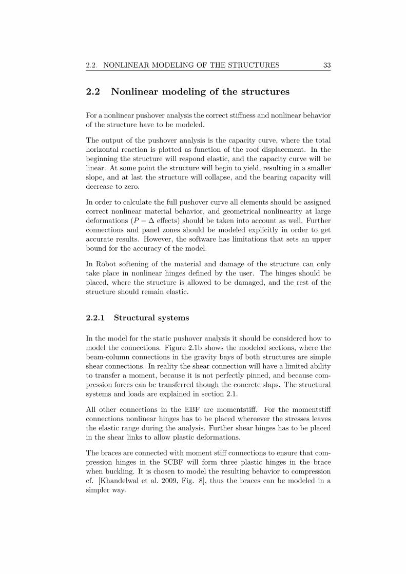
A general response spectrum is used to represent the seismic demand inseismic codes as [EN 1998-1:2004 2004] and [ATC-40 1996]. Robot uses theresponse spectrum from [ATC-40 1996], and generally seen it is like the onefrom [EN 1998-1:2004 2004] with a part with constant acceleration and apart with constant velocity, as shown in figure 2.4, where the peak groundacceleration is CA. If the period TS is equal to 0.4, as it is for a near sourcespectrum in [EN 1998-1:2004 2004] on hard rock, CV is equal to CA/2.5. In[EN 1998-1:2004 2004] the response spectrum has a last part with constantdisplacement for large periods.
Figure 2.4: General response spectrum from [ATC-40 1996].
2.2. NONLINEAR MODELING OF THE STRUCTURES 33
2.2 Nonlinear modeling of the structures
For a nonlinear pushover analysis the correct stiffness and nonlinear behaviorof the structure have to be modeled.
The output of the pushover analysis is the capacity curve, where the totalhorizontal reaction is plotted as function of the roof displacement. In thebeginning the structure will respond elastic, and the capacity curve will belinear. At some point the structure will begin to yield, resulting in a smallerslope, and at last the structure will collapse, and the bearing capacity willdecrease to zero.
In order to calculate the full pushover curve all elements should be assignedcorrect nonlinear material behavior, and geometrical nonlinearity at largedeformations (P −∆ effects) should be taken into account as well. Furtherconnections and panel zones should be modeled explicitly in order to getaccurate results. However, the software has limitations that sets an upperbound for the accuracy of the model.
In Robot softening of the material and damage of the structure can onlytake place in nonlinear hinges defined by the user. The hinges should beplaced, where the structure is allowed to be damaged, and the rest of thestructure should remain elastic.
2.2.1 Structural systems
In the model for the static pushover analysis it should be considered how tomodel the connections. Figure 2.1b shows the modeled sections, where thebeam-column connections in the gravity bays of both structures are simpleshear connections. In reality the shear connection will have a limited abilityto transfer a moment, because it is not perfectly pinned, and because com-pression forces can be transferred though the concrete slaps. The structuralsystems and loads are explained in section 2.1.
All other connections in the EBF are momentstiff. For the momentstiffconnections nonlinear hinges has to be placed whereever the stresses leavesthe elastic range during the analysis. Further shear hinges has to be placedin the shear links to allow plastic deformations.
The braces are connected with moment stiff connections to ensure that com-pression hinges in the SCBF will form three plastic hinges in the bracewhen buckling. It is chosen to model the resulting behavior to compressioncf. [Khandelwal et al. 2009, Fig. 8], thus the braces can be modeled in asimpler way.
34 CHAPTER 2. STRUCTURAL SEISMIC ANALYZES
2.2.2 Nonlinear hinges
In Robot there can only be defined one hinge in each node, thus if twobeams meets a column in the same point, there can only be defined a hingein one of them. To overcome this problem it may be necessary to place thehinge a bit away from the intersection point. For tension/compression bars,however this is not an option, since hinges can only be defined at the ends.
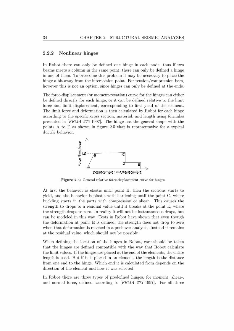
The force-displacement (or moment-rotation) curve for the hinges can eitherbe defined directly for each hinge, or it can be defined relative to the limitforce and limit displacement, corresponding to first yield of the element.The limit force and deformation is then calculated by Robot for each hingeaccording to the specific cross section, material, and length using formulaspresented in [FEMA 273 1997]. The hinge has the general shape with thepoints A to E as shown in figure 2.5 that is representative for a typicalductile behavior.
Figure 2.5: General relative force-displacement curve for hinges.
At first the behavior is elastic until point B, then the sections starts toyield, and the behavior is plastic with hardening until the point C, wherebuckling starts in the parts with compression or shear. This causes thestrength to drops to a residual value until it breaks at the point E, wherethe strength drops to zero. In reality it will not be instantaneous drops, butcan be modeled in this way. Tests in Robot have shown that even thoughthe deformation at point E is defined, the strength does not drop to zerowhen that deformation is reached in a pushover analysis. Instead it remainsat the residual value, which should not be possible.
When defining the location of the hinges in Robot, care should be takenthat the hinges are defined compatible with the way that Robot calculatethe limit values. If the hinges are placed at the end of the elements, the entirelength is used. But if it is placed in an element, the length is the distancefrom one end to the hinge. Which end it is calculated from depends on thedirection of the element and how it was selected.
In Robot there are three types of predefined hinges, for moment, shear-,and normal force, defined according to [FEMA 273 1997]. For all three
2.2. NONLINEAR MODELING OF THE STRUCTURES 35
types of hinges the force-displacement curve is linear from origo until thepoint where yielding begins, where the values are the limit displacementand the limit force. This limit displacement, however, corresponds to theelastic displacement, which takes place in the length of the element already.If the predefined hinges are used directly, the elastic deformation of theelements with hinges will be twice the size of those of a structure withouthinges, which is clearly wrong. Instead the hinges should be infinitely stiffuntil the limit force in reached, so that the only contribution is the plasticdeformation. To be able to find a numerical solution it is necessary to havesome slope though.
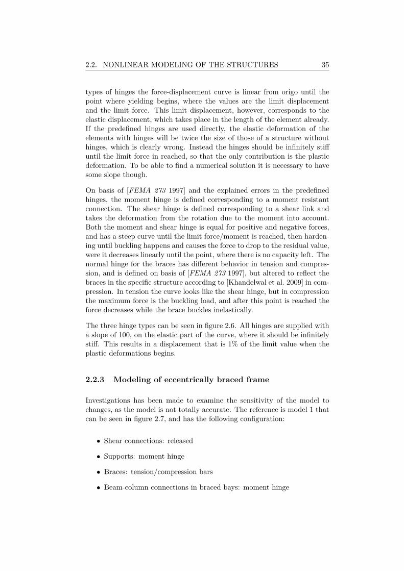
On basis of [FEMA 273 1997] and the explained errors in the predefinedhinges, the moment hinge is defined corresponding to a moment resistantconnection. The shear hinge is defined corresponding to a shear link andtakes the deformation from the rotation due to the moment into account.Both the moment and shear hinge is equal for positive and negative forces,and has a steep curve until the limit force/moment is reached, then harden-ing until buckling happens and causes the force to drop to the residual value,were it decreases linearly until the point, where there is no capacity left. Thenormal hinge for the braces has different behavior in tension and compres-sion, and is defined on basis of [FEMA 273 1997], but altered to reflect thebraces in the specific structure according to [Khandelwal et al. 2009] in com-pression. In tension the curve looks like the shear hinge, but in compressionthe maximum force is the buckling load, and after this point is reached theforce decreases while the brace buckles inelastically.
The three hinge types can be seen in figure 2.6. All hinges are supplied witha slope of 100, on the elastic part of the curve, where it should be infinitelystiff. This results in a displacement that is 1% of the limit value when theplastic deformations begins.
2.2.3 Modeling of eccentrically braced frame
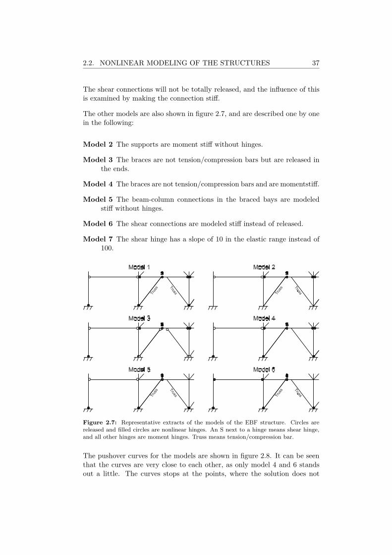
Investigations has been made to examine the sensitivity of the model tochanges, as the model is not totally accurate. The reference is model 1 thatcan be seen in figure 2.7, and has the following configuration:
• Shear connections: released
• Supports: moment hinge
• Braces: tension/compression bars
• Beam-column connections in braced bays: moment hinge
36 CHAPTER 2. STRUCTURAL SEISMIC ANALYZES
−6 −4 −2 0 2 4 6−1.5
−1
−0.5
0
0.5
1
1.5
Rotation/limit rotation
Mom
ent/l
imit
mom
ent
(a) Moment hinge with 2% hardening.
−20 −10 0 10 20−2
−1
0
1
2
Displacement/limit displacement
She
ar fo
rce/
limit
shea
r fo
rce
(b) Shear hinge with 3% hardening.
−10 −5 0 5 10 15−1.5
−1
−0.5
0
0.5
1
1.5
Displacement/limit displacement
Nor
mal
forc
e/lim
it no
rmal
forc
e
(c) Normal hinge with 2% tension hard-ening.
Figure 2.6: Force-displacement relationships for the hinges.
• Shear links: shear links in left side of the link
The hinges in the beam-column connection in the center bay is moved 1/100of the length of the beam towards the center, because two hinges cannot beplaced in the same point.
The moment and shear hinges are not modeled totally stiff until the limitrotation is reached because of convergence difficulties, and models are madeto examine the effect of this. This is done by replacing moment hinges withstiff connections. The shear hinges are not removed, because the nonlinearbehavior primarily takes place in those, instead it is made 10 times less stiff,to examine the influence of the stiffness.
In reality the braces are connected with stiff connections, but because thenonlinear compression behavior is taken into account with the shape of thehinge, the brace can be modeled as a tension/compression bar or a bar thatis released in the ends instead. The influence of the way it is modeled isexamined.
2.2. NONLINEAR MODELING OF THE STRUCTURES 37
The shear connections will not be totally released, and the influence of thisis examined by making the connection stiff.
The other models are also shown in figure 2.7, and are described one by onein the following:
Model 2 The supports are moment stiff without hinges.
Model 3 The braces are not tension/compression bars but are released inthe ends.
Model 4 The braces are not tension/compression bars and are momentstiff.
Model 5 The beam-column connections in the braced bays are modeledstiff without hinges.
Model 6 The shear connections are modeled stiff instead of released.
Model 7 The shear hinge has a slope of 10 in the elastic range instead of100.
Figure 2.7: Representative extracts of the models of the EBF structure. Circles arereleased and filled circles are nonlinear hinges. An S next to a hinge means shear hinge,and all other hinges are moment hinges. Truss means tension/compression bar.
The pushover curves for the models are shown in figure 2.8. It can be seenthat the curves are very close to each other, as only model 4 and 6 standsout a little. The curves stops at the points, where the solution does not
38 CHAPTER 2. STRUCTURAL SEISMIC ANALYZES
0 5 10 15 20 25 300
1000
2000
3000
4000
5000
6000
Displacement [cm]
She
ar fo
rce
[kN
]
1: Basis model2: Support: stiff3: Brace: released4: Brace: stiff5: Beam−column: stiff6: Shear connection: stiff7: Shear link: 0.1 hinge
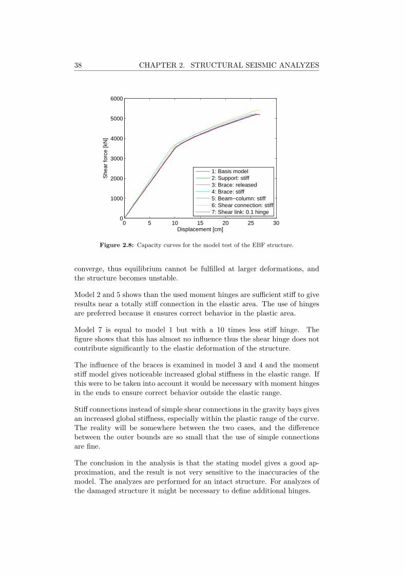
Figure 2.8: Capacity curves for the model test of the EBF structure.
converge, thus equilibrium cannot be fulfilled at larger deformations, andthe structure becomes unstable.
Model 2 and 5 shows than the used moment hinges are sufficient stiff to giveresults near a totally stiff connection in the elastic area. The use of hingesare preferred because it ensures correct behavior in the plastic area.
Model 7 is equal to model 1 but with a 10 times less stiff hinge. Thefigure shows that this has almost no influence thus the shear hinge does notcontribute significantly to the elastic deformation of the structure.
The influence of the braces is examined in model 3 and 4 and the momentstiff model gives noticeable increased global stiffness in the elastic range. Ifthis were to be taken into account it would be necessary with moment hingesin the ends to ensure correct behavior outside the elastic range.
Stiff connections instead of simple shear connections in the gravity bays givesan increased global stiffness, especially within the plastic range of the curve.The reality will be somewhere between the two cases, and the differencebetween the outer bounds are so small that the use of simple connectionsare fine.
The conclusion in the analysis is that the stating model gives a good ap-proximation, and the result is not very sensitive to the inaccuracies of themodel. The analyzes are performed for an intact structure. For analyzes ofthe damaged structure it might be necessary to define additional hinges.
2.2. NONLINEAR MODELING OF THE STRUCTURES 39
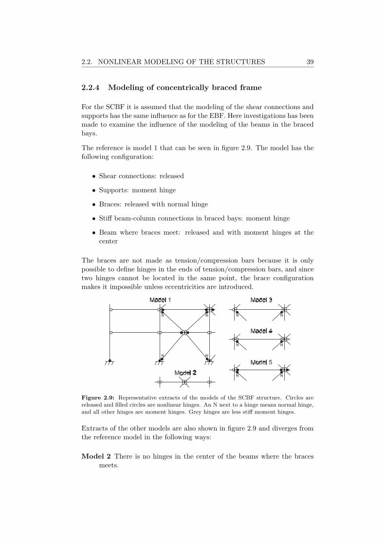
2.2.4 Modeling of concentrically braced frame
For the SCBF it is assumed that the modeling of the shear connections andsupports has the same influence as for the EBF. Here investigations has beenmade to examine the influence of the modeling of the beams in the bracedbays.
The reference is model 1 that can be seen in figure 2.9. The model has thefollowing configuration:
• Shear connections: released
• Supports: moment hinge
• Braces: released with normal hinge
• Stiff beam-column connections in braced bays: moment hinge
• Beam where braces meet: released and with moment hinges at thecenter
The braces are not made as tension/compression bars because it is onlypossible to define hinges in the ends of tension/compression bars, and sincetwo hinges cannot be located in the same point, the brace configurationmakes it impossible unless eccentricities are introduced.
Figure 2.9: Representative extracts of the models of the SCBF structure. Circles arereleased and filled circles are nonlinear hinges. An N next to a hinge means normal hinge,and all other hinges are moment hinges. Grey hinges are less stiff moment hinges.
Extracts of the other models are also shown in figure 2.9 and diverges fromthe reference model in the following ways:
Model 2 There is no hinges in the center of the beams where the bracesmeets.
40 CHAPTER 2. STRUCTURAL SEISMIC ANALYZES
Model 3 The stiff beam-column connections are modeled stiff without hinges.
Model 4 The stiff beam-column connections are modeled with hinges thathave a slope in the elastic range of 1.
Model 5 The stiff beam-column connections are modeled as released.
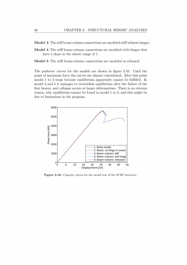
The pushover curves for the models are shown in figure 2.10. Until thepoint of maximum force the curves are almost coincidental. After this pointmodel 1 to 3 stops because equilibrium apparently cannot be fulfilled. Inmodel 4 and 5 it manages to reestablish equilibrium after the failure of thefirst braces, and collapse occurs at larger deformations. There is no obviousreason, why equilibrium cannot be found in model 1 to 3, and this might bedue to limitations in the program.
0 5 10 15 20 25 30 35 400
1000
2000
3000
4000
5000
6000
Displacement [cm]
She
ar fo
rce
[kN
]
1: Basis model2: Beam: no hinge in centre3: Beam−column: stiff4: Beam−column: soft hinge5: Beam−column: released
Figure 2.10: Capacity curves for the model test of the SCBF structure.
2.3. PERFORMANCE OF STRUCTURES 41
2.3 Performance of structures
In this section the performance of the structures at the earthquake with 2%probability of occurrence in 50 years is found, and the nonlinear behavior isinvestigated. Forces and deformations originating from the lateral force isinvestigated, but the influence of the vertical load from self and live load isnot taken into account due to limitations in the program.
2.3.1 Eccentrically braced frame
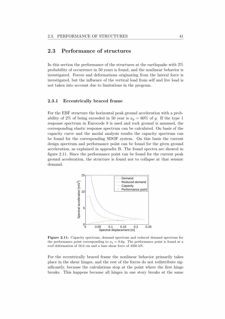
For the EBF structure the horizontal peak ground acceleration with a prob-ability of 2% of being exceeded in 50 year is ag = 60% of g. If the type 1response spectrum in Eurocode 8 is used and rock ground is assumed, thecorresponding elastic response spectrum can be calculated. On basis of thecapacity curve and the modal analysis results the capacity spectrum canbe found for the corresponding SDOF system. On this basis the currentdesign spectrum and performance point can be found for the given groundacceleration, as explained in appendix B. The found spectra are showed infigure 2.11. Since the performance point can be found for the current peakground acceleration, the structure is found not to collapse at that seismicdemand.
0 0.05 0.1 0.15 0.2 0.250
5
10
15
Spectral displacement [m]
Spe
ctra
l acc
eler
atio
n [m
/s2 ]
DemandReduced demandCapacityPerformance point
Figure 2.11: Capacity spectrum, demand spectrum and reduced demand spectrum forthe performance point corresponding to ag = 0.6g. The performance point is found at aroof deformation of 16.6 cm and a base shear force of 4356 kN.
For the eccentrically braced frame the nonlinear behavior primarily takesplace in the shear hinges, and the rest of the forces do not redistribute sig-nificantly, because the calculations stop at the point where the first hingebreaks. This happens because all hinges in one story breaks at the same
42 CHAPTER 2. STRUCTURAL SEISMIC ANALYZES
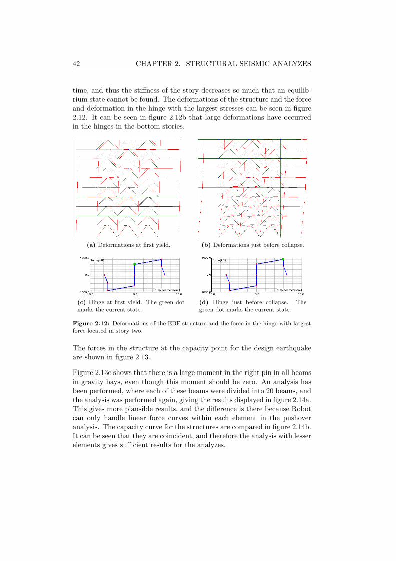
time, and thus the stiffness of the story decreases so much that an equilib-rium state cannot be found. The deformations of the structure and the forceand deformation in the hinge with the largest stresses can be seen in figure2.12. It can be seen in figure 2.12b that large deformations have occurredin the hinges in the bottom stories.
(a) Deformations at first yield. (b) Deformations just before collapse.
(c) Hinge at first yield. The green dotmarks the current state.
(d) Hinge just before collapse. Thegreen dot marks the current state.
Figure 2.12: Deformations of the EBF structure and the force in the hinge with largestforce located in story two.
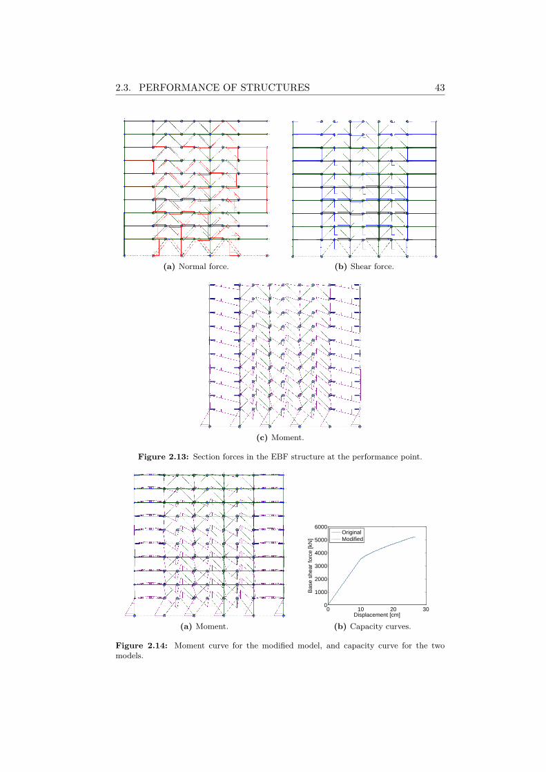
The forces in the structure at the capacity point for the design earthquakeare shown in figure 2.13.
Figure 2.13c shows that there is a large moment in the right pin in all beamsin gravity bays, even though this moment should be zero. An analysis hasbeen performed, where each of these beams were divided into 20 beams, andthe analysis was performed again, giving the results displayed in figure 2.14a.This gives more plausible results, and the difference is there because Robotcan only handle linear force curves within each element in the pushoveranalysis. The capacity curve for the structures are compared in figure 2.14b.It can be seen that they are coincident, and therefore the analysis with lesserelements gives sufficient results for the analyzes.
2.3. PERFORMANCE OF STRUCTURES 43
(a) Normal force. (b) Shear force.
(c) Moment.
Figure 2.13: Section forces in the EBF structure at the performance point.
(a) Moment.
0 10 20 300
1000
2000
3000
4000
5000
6000
Displacement [cm]
Bas
e sh
ear
forc
e [k
N]
OriginalModified
(b) Capacity curves.
Figure 2.14: Moment curve for the modified model, and capacity curve for the twomodels.
44 CHAPTER 2. STRUCTURAL SEISMIC ANALYZES
2.3.2 Concentrically braced frame
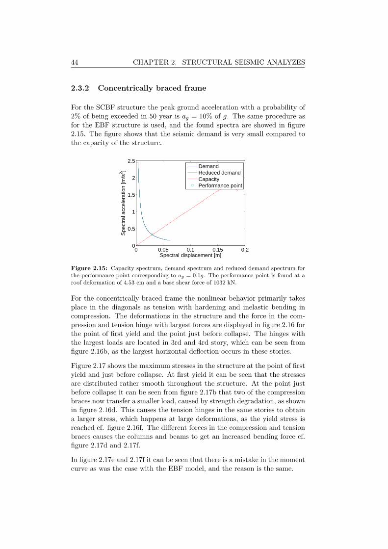
For the SCBF structure the peak ground acceleration with a probability of2% of being exceeded in 50 year is ag = 10% of g. The same procedure asfor the EBF structure is used, and the found spectra are showed in figure2.15. The figure shows that the seismic demand is very small compared tothe capacity of the structure.
0 0.05 0.1 0.15 0.20
0.5
1
1.5
2
2.5
Spectral displacement [m]
Spe
ctra
l acc
eler
atio
n [m
/s2 ]
DemandReduced demandCapacityPerformance point
Figure 2.15: Capacity spectrum, demand spectrum and reduced demand spectrum forthe performance point corresponding to ag = 0.1g. The performance point is found at aroof deformation of 4.53 cm and a base shear force of 1032 kN.
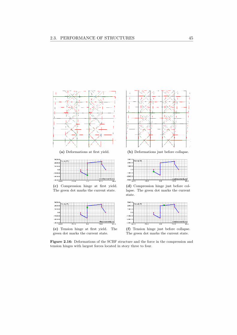
For the concentrically braced frame the nonlinear behavior primarily takesplace in the diagonals as tension with hardening and inelastic bending incompression. The deformations in the structure and the force in the com-pression and tension hinge with largest forces are displayed in figure 2.16 forthe point of first yield and the point just before collapse. The hinges withthe largest loads are located in 3rd and 4rd story, which can be seen fromfigure 2.16b, as the largest horizontal deflection occurs in these stories.
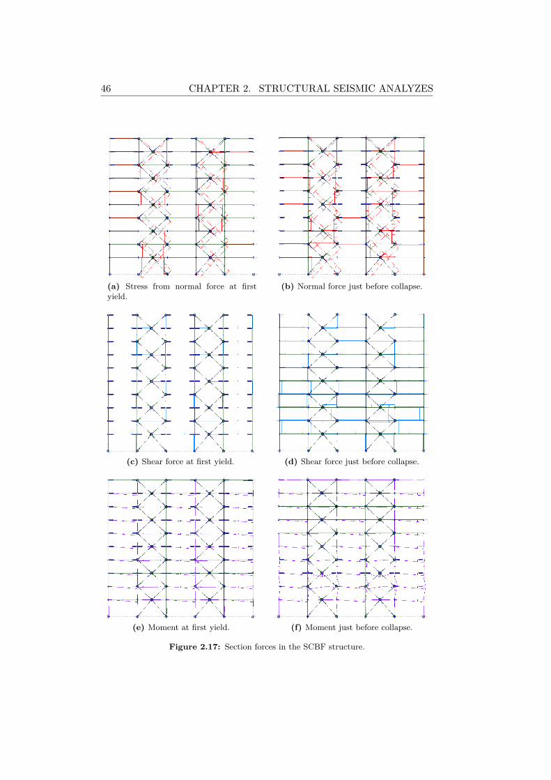
Figure 2.17 shows the maximum stresses in the structure at the point of firstyield and just before collapse. At first yield it can be seen that the stressesare distributed rather smooth throughout the structure. At the point justbefore collapse it can be seen from figure 2.17b that two of the compressionbraces now transfer a smaller load, caused by strength degradation, as shownin figure 2.16d. This causes the tension hinges in the same stories to obtaina larger stress, which happens at large deformations, as the yield stress isreached cf. figure 2.16f. The different forces in the compression and tensionbraces causes the columns and beams to get an increased bending force cf.figure 2.17d and 2.17f.
In figure 2.17e and 2.17f it can be seen that there is a mistake in the momentcurve as was the case with the EBF model, and the reason is the same.
2.3. PERFORMANCE OF STRUCTURES 45
(a) Deformations at first yield. (b) Deformations just before collapse.
(c) Compression hinge at first yield.The green dot marks the current state.
(d) Compression hinge just before col-lapse. The green dot marks the currentstate.
(e) Tension hinge at first yield. Thegreen dot marks the current state.
(f) Tension hinge just before collapse.The green dot marks the current state.
Figure 2.16: Deformations of the SCBF structure and the force in the compression andtension hinges with largest forces located in story three to four.
46 CHAPTER 2. STRUCTURAL SEISMIC ANALYZES
(a) Stress from normal force at firstyield.
(b) Normal force just before collapse.
(c) Shear force at first yield. (d) Shear force just before collapse.
(e) Moment at first yield. (f) Moment just before collapse.
Figure 2.17: Section forces in the SCBF structure.
2.4. SUMMARY 47
2.4 Summary
Two structures have been chosen for this analysis, an EBF located in Seattleand a SCBF located in Atlanta. A plane finite element model of each hasbeen made, and nonlinear hinges have been placed to ensure the correctnonlinear behavior. More different models have been made to investigatethe sensitivity of the pushover curve towards minor changes in the models.
The EBF was found to have a ductile behavior and it collapses at the point,where all shear hinges in one story fail. For the SCBF equilibrium couldnot be found after the failure of the first compression braces except for twoof the alternate models, where the moment connections were less stiff. Thisindicates that it might be due to limitations in the program that the struc-ture does not retain some strength after the failure of the first compressionhinges.
The performance of structures was found for earthquakes with 2% proba-bility of occurrence in 50 years for the respective locations. Both structureswere found to have sufficient capacity using the performance based methodin [ATC-40 1996], and the SCBF had a capacity much higher than necessaryfor the given earthquake.

48 CHAPTER 2. STRUCTURAL SEISMIC ANALYZES
Chapter 3
Assessment of robustness
In this chapter the robustness of the structures is evaluated through a qual-itative discussion and through deterministic analyzes.
3.1 Structural configuration
In section 1.2.1 different strategies to ensure the robustness were discussed.The robustness of the structures is evaluated through a discussion of thethree different strategies:
• Redundancy and ductility
• Isolation by compartmentalization
• Design of key elements
3.1.1 Redundancy and ductility
Redundancy and ductility are two properties of a structure that is able toprovide alternate load paths if damaged. The structures, cf. section 2.1,are made of steel that is a highly ductile material, and are able to absorblarge deformations without breaking. The braced bays of the structures areseveral times statically undetermined, and thus it might be able to providealternate load paths if damaged.
The progressive collapse behavior of the structures was studied by [Khandelwalet al. 2009], and they found the structures capable of providing alternate load
49
50 CHAPTER 3. ASSESSMENT OF ROBUSTNESS
paths in most cases. For the SCBF structure they found that the Achillesheel was the corner columns. This is quite obvious because they are nothold by any brace, and all beam-column connections are shear connections.If the column in the lower story is damaged or removed, only the concreteslaps that will work as cantilevers, and the very limited moment capacity ofthe shear connections can help the corner bays from collapsing.
The same is the case for the interior columns, where there are no braceseither. But because the slaps are supported in the entire perimeter by theintact columns, they will be able to hold a larger load because this will givea smaller moment and due to the membrane forces in the slap.
An alternative system, where at least one braced bay was placed next toall outer columns, would eliminate the problem with the corner columns.Alternatively the robustness might be increased by making moment resistantconnections instead of shear connections. This will increase the number ofalternate load paths and increase the stiffness of the structure. But it mightnot be a good system, since it might require larger beams and it will increasethe loading of the columns.
3.1.2 Isolation by compartmentalization
Isolation by compartmentalization is a strategy that allows a partial collapseof the structure with the aim of avoiding a complete collapse. If ”removalof column”-scenarios are examined it might be necessary to allow a bay tocollapse in the entire height of the building, if that strategy is to be used.It might be relevant in connection with the corner columns that are notsupported by braces. Due to this strategy, the corner bay should be allowedto break like in the case of Ronan Point, to save the remaining structure.But failure of the corner bays in the entire height of the structure will stillbe disproportionate, when the local damage is only one column, and it isnot an acceptable damage.
In addition the strategy will not help much if the resistance against hori-zontal loads is investigated. The seismic load will be a little bit smaller,since the mass is smaller, but unless a larger part of the structure is al-lowed to collapse, the influence will be infinitesimal. Further it will be hardto implement in this type of structure, without a general weakening of thestructure.
3.2. BEHAVIOR OF DAMAGED SYSTEMS 51
3.1.3 Design of key elements
If the structure contains key elements the partial factor on these can beincreased with a factor 1.2 to increase the overall safety of the structure.For the current structures it might be relevant to regard the corner columnsthat are not next to a braced bay in any direction, as key elements. Sincethe columns in general are designed with respect to the principle of strongcolumn-weak beam (capacity design) they might already be oversized fortheir design loads.
3.2 Behavior of damaged systems
The robustness can be evaluated on basis of the capacity of the intact systemversus the capacity of a damaged structure, where a limited part of thestructure is removed (eg a column and adjoining braces). In this projectonly the resistance against horizontal load is evaluated, as the resistanceagainst vertical load was studied by [Khandelwal et al. 2009]. The capacityagainst horizontal load is found through a pushover analysis, and the verticalload is not taken into account in the analysis because of limitations in theprogram.
In this analysis different scenarios are investigated, where a column and ad-joining braces in the lower story is removed, and the capacity is found. Theconsidered facades has six columns, and thus six different damage scenariosare possible. The corner columns in the SCBF, however, are key elementsas they are placed next to gravity bays, and removal of those columns wouldresult in an instable model, where the gravity bay is movable, and where thecapacity of the rest of the model would not be changed significantly. For theEBF the corner columns are hold by braces in the other direction, but sincethe model is plane it would not make sense to remove them in this analysis.Further the structures are symmetric, and only two basically different sce-narios are possible. Those are referred to as Damage1 and Damage2, andcan be seen in figure 3.1.
Three different limit states for the structure as system are investigated, withdefinitions from [Ellingwood & Kinali 2009]:
• Immediate Occupancy (IO):Onset of inelastic behavior
• Structural Damage (SD):Global lateral stiffness drops to half of initial value
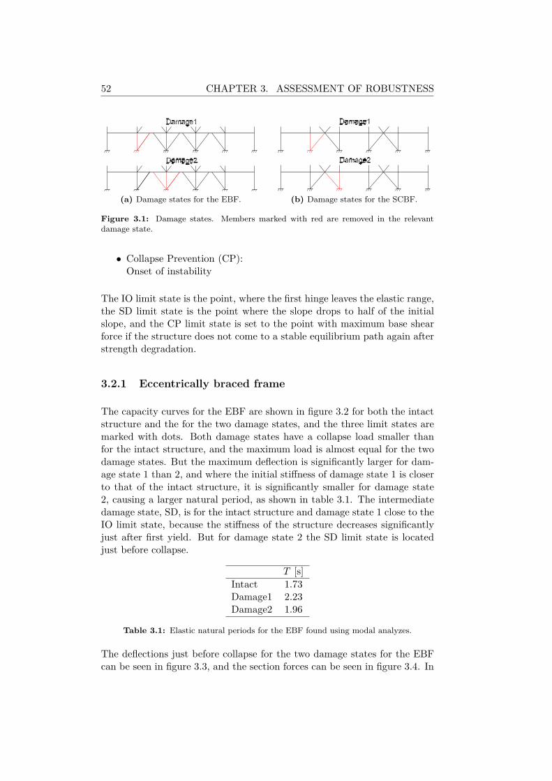
52 CHAPTER 3. ASSESSMENT OF ROBUSTNESS
(a) Damage states for the EBF. (b) Damage states for the SCBF.
Figure 3.1: Damage states. Members marked with red are removed in the relevantdamage state.
• Collapse Prevention (CP):Onset of instability
The IO limit state is the point, where the first hinge leaves the elastic range,the SD limit state is the point where the slope drops to half of the initialslope, and the CP limit state is set to the point with maximum base shearforce if the structure does not come to a stable equilibrium path again afterstrength degradation.
3.2.1 Eccentrically braced frame
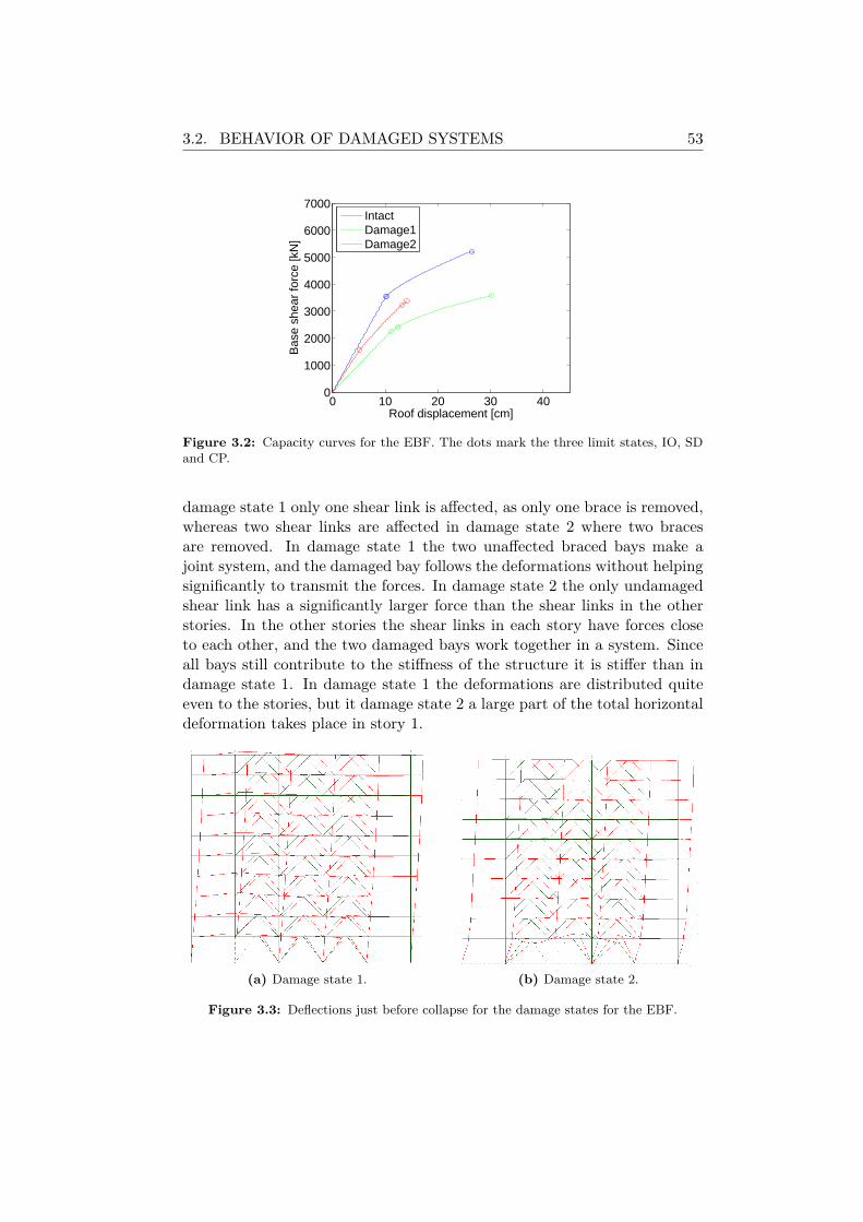
The capacity curves for the EBF are shown in figure 3.2 for both the intactstructure and the for the two damage states, and the three limit states aremarked with dots. Both damage states have a collapse load smaller thanfor the intact structure, and the maximum load is almost equal for the twodamage states. But the maximum deflection is significantly larger for dam-age state 1 than 2, and where the initial stiffness of damage state 1 is closerto that of the intact structure, it is significantly smaller for damage state2, causing a larger natural period, as shown in table 3.1. The intermediatedamage state, SD, is for the intact structure and damage state 1 close to theIO limit state, because the stiffness of the structure decreases significantlyjust after first yield. But for damage state 2 the SD limit state is locatedjust before collapse.
T [s]Intact 1.73Damage1 2.23Damage2 1.96
Table 3.1: Elastic natural periods for the EBF found using modal analyzes.
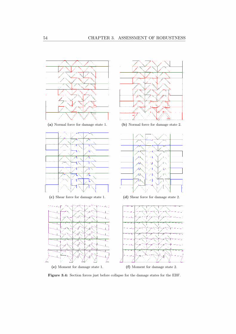
The deflections just before collapse for the two damage states for the EBFcan be seen in figure 3.3, and the section forces can be seen in figure 3.4. In
3.2. BEHAVIOR OF DAMAGED SYSTEMS 53
0 10 20 30 400
1000
2000
3000
4000
5000
6000
7000
Roof displacement [cm]
Bas
e sh
ear
forc
e [k
N]
IntactDamage1Damage2
Figure 3.2: Capacity curves for the EBF. The dots mark the three limit states, IO, SDand CP.
damage state 1 only one shear link is affected, as only one brace is removed,whereas two shear links are affected in damage state 2 where two bracesare removed. In damage state 1 the two unaffected braced bays make ajoint system, and the damaged bay follows the deformations without helpingsignificantly to transmit the forces. In damage state 2 the only undamagedshear link has a significantly larger force than the shear links in the otherstories. In the other stories the shear links in each story have forces closeto each other, and the two damaged bays work together in a system. Sinceall bays still contribute to the stiffness of the structure it is stiffer than indamage state 1. In damage state 1 the deformations are distributed quiteeven to the stories, but it damage state 2 a large part of the total horizontaldeformation takes place in story 1.
(a) Damage state 1. (b) Damage state 2.
Figure 3.3: Deflections just before collapse for the damage states for the EBF.
54 CHAPTER 3. ASSESSMENT OF ROBUSTNESS
(a) Normal force for damage state 1. (b) Normal force for damage state 2.
(c) Shear force for damage state 1. (d) Shear force for damage state 2.
(e) Moment for damage state 1. (f) Moment for damage state 2.
Figure 3.4: Section forces just before collapse for the damage states for the EBF.
3.2. BEHAVIOR OF DAMAGED SYSTEMS 55
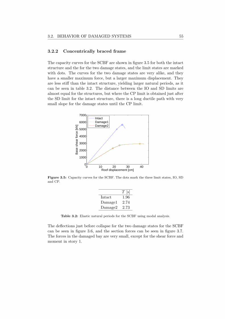
3.2.2 Concentrically braced frame
The capacity curves for the SCBF are shown in figure 3.5 for both the intactstructure and the for the two damage states, and the limit states are markedwith dots. The curves for the two damage states are very alike, and theyhave a smaller maximum force, but a larger maximum displacement. Theyare less stiff than the intact structure, yielding larger natural periods, as itcan be seen in table 3.2. The distance between the IO and SD limits arealmost equal for the structures, but where the CP limit is obtained just afterthe SD limit for the intact structure, there is a long ductile path with verysmall slope for the damage states until the CP limit.
0 10 20 30 400
1000
2000
3000
4000
5000
6000
7000
Roof displacement [cm]
Bas
e sh
ear
forc
e [k
N]
IntactDamage1Damage2
Figure 3.5: Capacity curves for the SCBF. The dots mark the three limit states, IO, SDand CP.
T [s]Intact 1.96Damage1 2.74Damage2 2.73
Table 3.2: Elastic natural periods for the SCBF using modal analysis.
The deflections just before collapse for the two damage states for the SCBFcan be seen in figure 3.6, and the section forces can be seen in figure 3.7.The forces in the damaged bay are very small, except for the shear force andmoment in story 1.
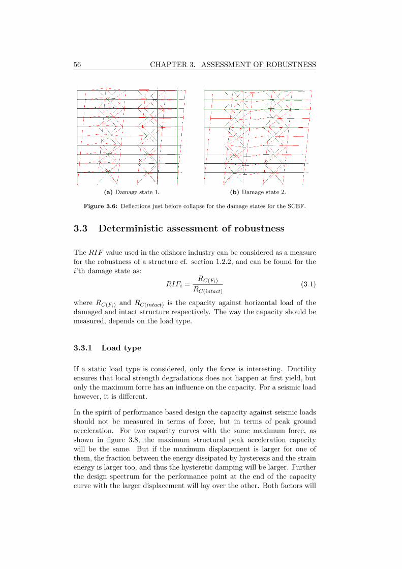
56 CHAPTER 3. ASSESSMENT OF ROBUSTNESS
(a) Damage state 1. (b) Damage state 2.
Figure 3.6: Deflections just before collapse for the damage states for the SCBF.
3.3 Deterministic assessment of robustness
The RIF value used in the offshore industry can be considered as a measurefor the robustness of a structure cf. section 1.2.2, and can be found for thei’th damage state as:
RIFi =RC(Fi)RC(intact)
(3.1)
where RC(Fi) and RC(intact) is the capacity against horizontal load of thedamaged and intact structure respectively. The way the capacity should bemeasured, depends on the load type.
3.3.1 Load type
If a static load type is considered, only the force is interesting. Ductilityensures that local strength degradations does not happen at first yield, butonly the maximum force has an influence on the capacity. For a seismic loadhowever, it is different.
In the spirit of performance based design the capacity against seismic loadsshould not be measured in terms of force, but in terms of peak groundacceleration. For two capacity curves with the same maximum force, asshown in figure 3.8, the maximum structural peak acceleration capacitywill be the same. But if the maximum displacement is larger for one ofthem, the fraction between the energy dissipated by hysteresis and the strainenergy is larger too, and thus the hysteretic damping will be larger. Furtherthe design spectrum for the performance point at the end of the capacitycurve with the larger displacement will lay over the other. Both factors will
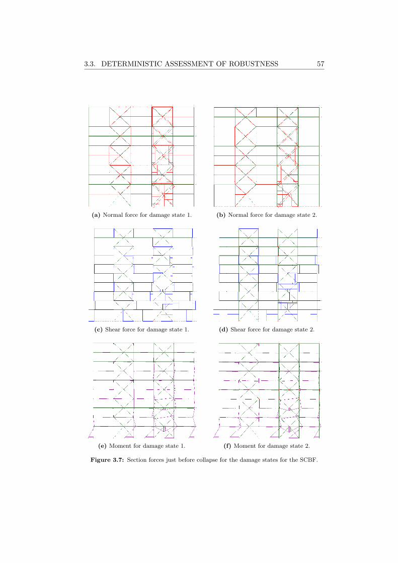
3.3. DETERMINISTIC ASSESSMENT OF ROBUSTNESS 57
(a) Normal force for damage state 1. (b) Normal force for damage state 2.
(c) Shear force for damage state 1. (d) Shear force for damage state 2.
(e) Moment for damage state 1. (f) Moment for damage state 2.
Figure 3.7: Section forces just before collapse for the damage states for the SCBF.
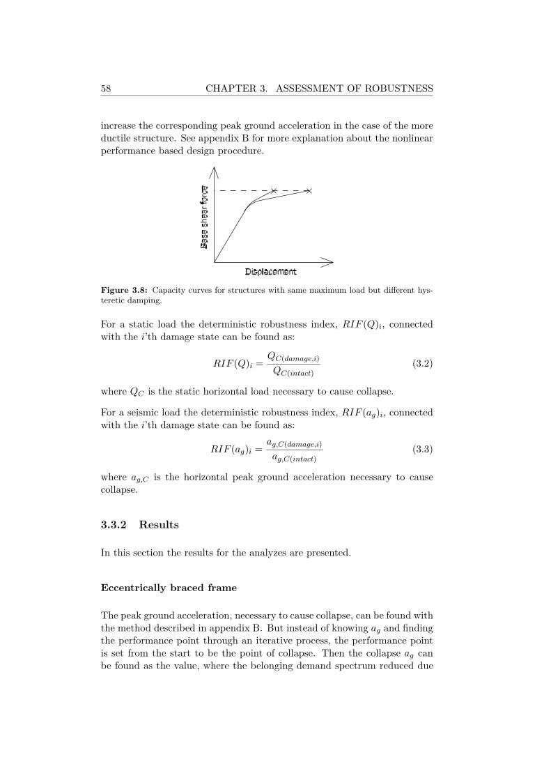
58 CHAPTER 3. ASSESSMENT OF ROBUSTNESS
increase the corresponding peak ground acceleration in the case of the moreductile structure. See appendix B for more explanation about the nonlinearperformance based design procedure.
Figure 3.8: Capacity curves for structures with same maximum load but different hys-teretic damping.
For a static load the deterministic robustness index, RIF (Q)i, connectedwith the i’th damage state can be found as:
RIF (Q)i =QC(damage,i)QC(intact)
(3.2)
where QC is the static horizontal load necessary to cause collapse.
For a seismic load the deterministic robustness index, RIF (ag)i, connectedwith the i’th damage state can be found as:
RIF (ag)i =ag,C(damage,i)ag,C(intact)
(3.3)
where ag,C is the horizontal peak ground acceleration necessary to causecollapse.
3.3.2 Results
In this section the results for the analyzes are presented.
Eccentrically braced frame
The peak ground acceleration, necessary to cause collapse, can be found withthe method described in appendix B. But instead of knowing ag and findingthe performance point through an iterative process, the performance pointis set from the start to be the point of collapse. Then the collapse ag canbe found as the value, where the belonging demand spectrum reduced due
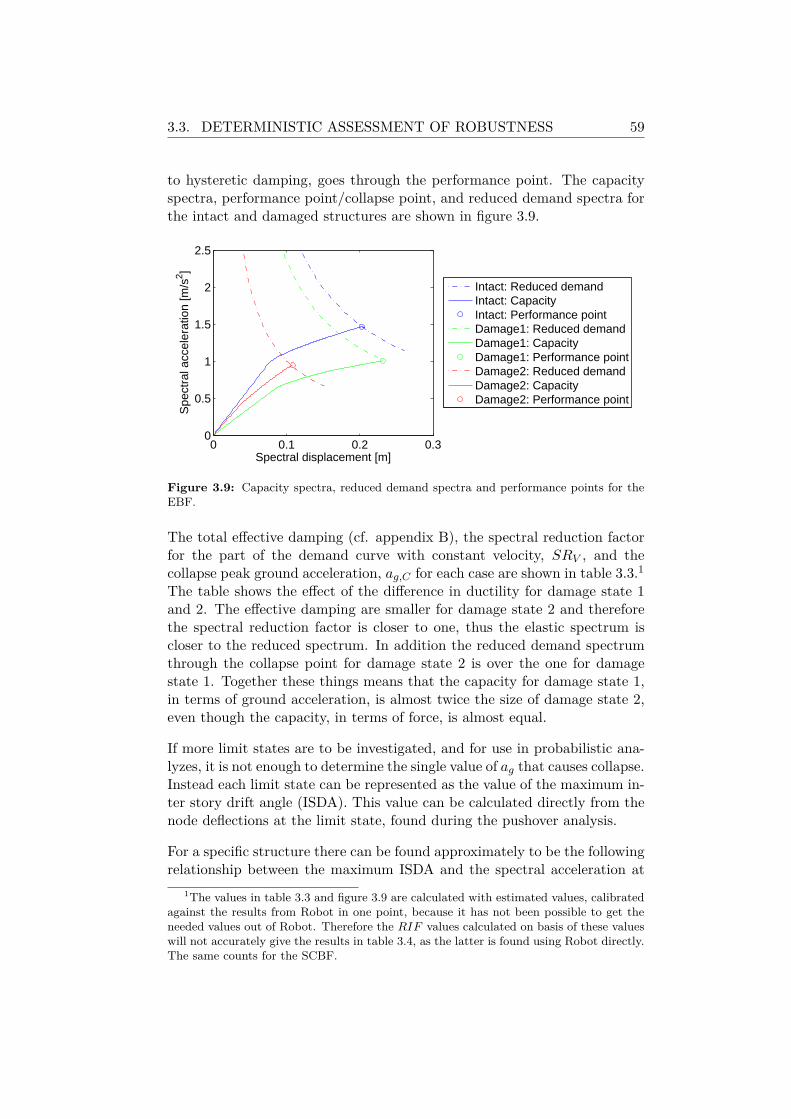
3.3. DETERMINISTIC ASSESSMENT OF ROBUSTNESS 59
to hysteretic damping, goes through the performance point. The capacityspectra, performance point/collapse point, and reduced demand spectra forthe intact and damaged structures are shown in figure 3.9.
0 0.1 0.2 0.30
0.5
1
1.5
2
2.5
Spectral displacement [m]
Spe
ctra
l acc
eler
atio
n [m
/s2 ]
Intact: Reduced demandIntact: CapacityIntact: Performance pointDamage1: Reduced demandDamage1: CapacityDamage1: Performance pointDamage2: Reduced demandDamage2: CapacityDamage2: Performance point
Figure 3.9: Capacity spectra, reduced demand spectra and performance points for theEBF.
The total effective damping (cf. appendix B), the spectral reduction factorfor the part of the demand curve with constant velocity, SRV , and thecollapse peak ground acceleration, ag,C for each case are shown in table 3.3.1The table shows the effect of the difference in ductility for damage state 1and 2. The effective damping are smaller for damage state 2 and thereforethe spectral reduction factor is closer to one, thus the elastic spectrum iscloser to the reduced spectrum. In addition the reduced demand spectrumthrough the collapse point for damage state 2 is over the one for damagestate 1. Together these things means that the capacity for damage state 1,in terms of ground acceleration, is almost twice the size of damage state 2,even though the capacity, in terms of force, is almost equal.
If more limit states are to be investigated, and for use in probabilistic ana-lyzes, it is not enough to determine the single value of ag that causes collapse.Instead each limit state can be represented as the value of the maximum in-ter story drift angle (ISDA). This value can be calculated directly from thenode deflections at the limit state, found during the pushover analysis.
For a specific structure there can be found approximately to be the followingrelationship between the maximum ISDA and the spectral acceleration at
1The values in table 3.3 and figure 3.9 are calculated with estimated values, calibratedagainst the results from Robot in one point, because it has not been possible to get theneeded values out of Robot. Therefore the RIF values calculated on basis of these valueswill not accurately give the results in table 3.4, as the latter is found using Robot directly.The same counts for the SCBF.
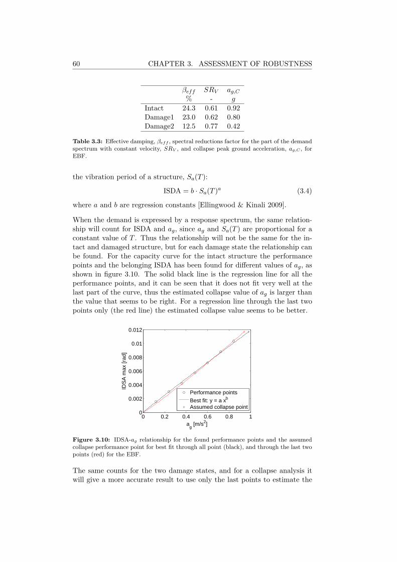
60 CHAPTER 3. ASSESSMENT OF ROBUSTNESS
βeff SRV ag,C% - g
Intact 24.3 0.61 0.92Damage1 23.0 0.62 0.80Damage2 12.5 0.77 0.42
Table 3.3: Effective damping, βeff , spectral reductions factor for the part of the demandspectrum with constant velocity, SRV , and collapse peak ground acceleration, ag,C , forEBF.
the vibration period of a structure, Sa(T ):
ISDA = b · Sa(T )a (3.4)
where a and b are regression constants [Ellingwood & Kinali 2009].
When the demand is expressed by a response spectrum, the same relation-ship will count for ISDA and ag, since ag and Sa(T ) are proportional for aconstant value of T . Thus the relationship will not be the same for the in-tact and damaged structure, but for each damage state the relationship canbe found. For the capacity curve for the intact structure the performancepoints and the belonging ISDA has been found for different values of ag, asshown in figure 3.10. The solid black line is the regression line for all theperformance points, and it can be seen that it does not fit very well at thelast part of the curve, thus the estimated collapse value of ag is larger thanthe value that seems to be right. For a regression line through the last twopoints only (the red line) the estimated collapse value seems to be better.
0 0.2 0.4 0.6 0.8 10
0.002
0.004
0.006
0.008
0.01
0.012
ag [m/s2]
IDS
A m
ax [r
ad]
Performance points
Best fit: y = a xb
Assumed collapse point
Figure 3.10: IDSA-ag relationship for the found performance points and the assumedcollapse performance point for best fit through all point (black), and through the last twopoints (red) for the EBF.
The same counts for the two damage states, and for a collapse analysis itwill give a more accurate result to use only the last points to estimate the
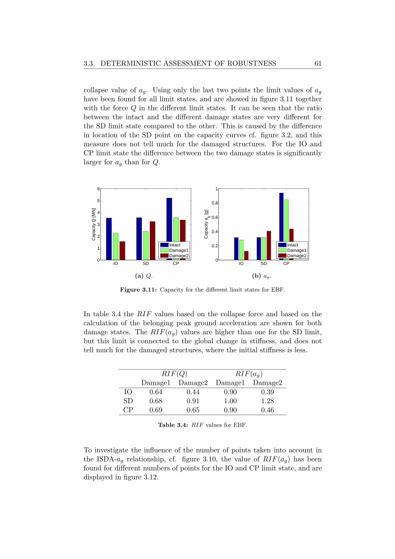
3.3. DETERMINISTIC ASSESSMENT OF ROBUSTNESS 61
collapse value of ag. Using only the last two points the limit values of aghave been found for all limit states, and are showed in figure 3.11 togetherwith the force Q in the different limit states. It can be seen that the ratiobetween the intact and the different damage states are very different forthe SD limit state compared to the other. This is caused by the differencein location of the SD point on the capacity curves cf. figure 3.2, and thismeasure does not tell much for the damaged structures. For the IO andCP limit state the difference between the two damage states is significantlylarger for ag than for Q.
IO SD CP0
1
2
3
4
5
6
Cap
acity
Q [M
N]
IntactDamage1Damage2
(a) Q.
IO SD CP0
0.2
0.4
0.6
0.8
1
Cap
acity
ag [g
]
IntactDamage1Damage2
(b) ag.
Figure 3.11: Capacity for the different limit states for EBF.
In table 3.4 the RIF values based on the collapse force and based on thecalculation of the belonging peak ground acceleration are shown for bothdamage states. The RIF (ag) values are higher than one for the SD limit,but this limit is connected to the global change in stiffness, and does nottell much for the damaged structures, where the initial stiffness is less.
RIF (Q) RIF (ag)Damage1 Damage2 Damage1 Damage2
IO 0.64 0.44 0.90 0.39SD 0.68 0.91 1.00 1.28CP 0.69 0.65 0.90 0.46
Table 3.4: RIF values for EBF.
To investigate the influence of the number of points taken into account inthe ISDA-ag relationship, cf. figure 3.10, the value of RIF (ag) has beenfound for different numbers of points for the IO and CP limit state, and aredisplayed in figure 3.12.
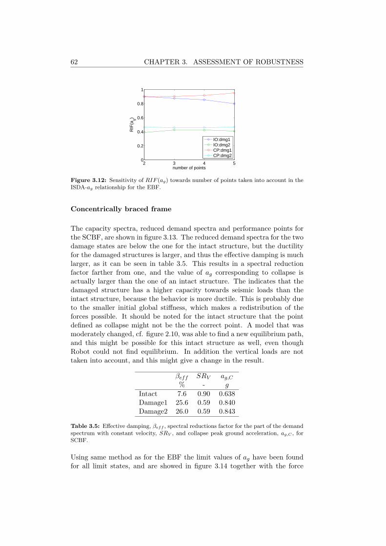
62 CHAPTER 3. ASSESSMENT OF ROBUSTNESS
2 3 4 50
0.2
0.4
0.6
0.8
1
number of points
RIF
(ag)
IO:dmg1IO:dmg2CP:dmg1CP:dmg2
Figure 3.12: Sensitivity of RIF (ag) towards number of points taken into account in theISDA-ag relationship for the EBF.
Concentrically braced frame
The capacity spectra, reduced demand spectra and performance points forthe SCBF, are shown in figure 3.13. The reduced demand spectra for the twodamage states are below the one for the intact structure, but the ductilityfor the damaged structures is larger, and thus the effective damping is muchlarger, as it can be seen in table 3.5. This results in a spectral reductionfactor farther from one, and the value of ag corresponding to collapse isactually larger than the one of an intact structure. The indicates that thedamaged structure has a higher capacity towards seismic loads than theintact structure, because the behavior is more ductile. This is probably dueto the smaller initial global stiffness, which makes a redistribution of theforces possible. It should be noted for the intact structure that the pointdefined as collapse might not be the the correct point. A model that wasmoderately changed, cf. figure 2.10, was able to find a new equilibrium path,and this might be possible for this intact structure as well, even thoughRobot could not find equilibrium. In addition the vertical loads are nottaken into account, and this might give a change in the result.
βeff SRV ag,C% - g
Intact 7.6 0.90 0.638Damage1 25.6 0.59 0.840Damage2 26.0 0.59 0.843
Table 3.5: Effective damping, βeff , spectral reductions factor for the part of the demandspectrum with constant velocity, SRV , and collapse peak ground acceleration, ag,C , forSCBF.
Using same method as for the EBF the limit values of ag have been foundfor all limit states, and are showed in figure 3.14 together with the force
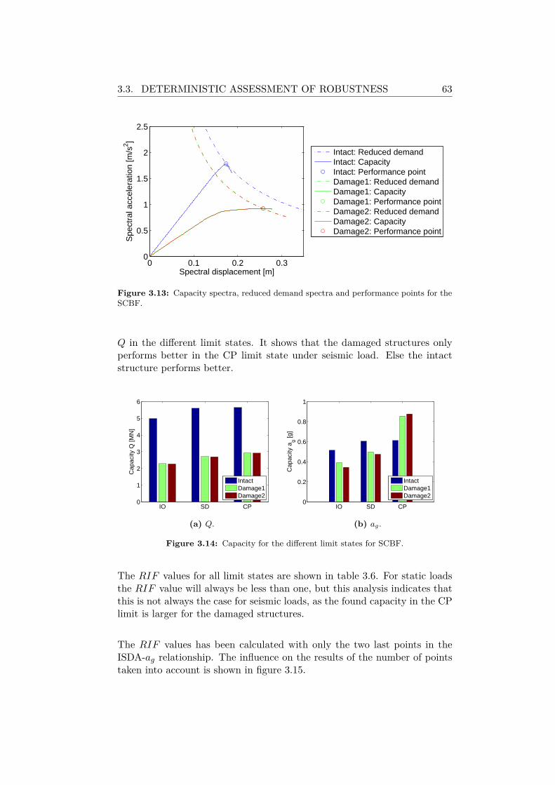
3.3. DETERMINISTIC ASSESSMENT OF ROBUSTNESS 63
0 0.1 0.2 0.30
0.5
1
1.5
2
2.5
Spectral displacement [m]
Spe
ctra
l acc
eler
atio
n [m
/s2 ]
Intact: Reduced demandIntact: CapacityIntact: Performance pointDamage1: Reduced demandDamage1: CapacityDamage1: Performance pointDamage2: Reduced demandDamage2: CapacityDamage2: Performance point
Figure 3.13: Capacity spectra, reduced demand spectra and performance points for theSCBF.
Q in the different limit states. It shows that the damaged structures onlyperforms better in the CP limit state under seismic load. Else the intactstructure performs better.
IO SD CP0
1
2
3
4
5
6
Cap
acity
Q [M
N]
IntactDamage1Damage2
(a) Q.
IO SD CP0
0.2
0.4
0.6
0.8
1
Cap
acity
ag [g
]
IntactDamage1Damage2
(b) ag.
Figure 3.14: Capacity for the different limit states for SCBF.
The RIF values for all limit states are shown in table 3.6. For static loadsthe RIF value will always be less than one, but this analysis indicates thatthis is not always the case for seismic loads, as the found capacity in the CPlimit is larger for the damaged structures.
The RIF values has been calculated with only the two last points in theISDA-ag relationship. The influence on the results of the number of pointstaken into account is shown in figure 3.15.
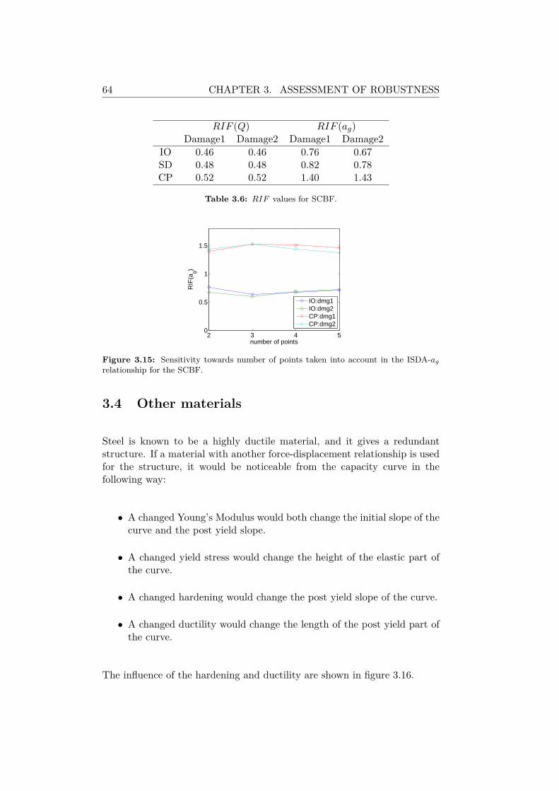
64 CHAPTER 3. ASSESSMENT OF ROBUSTNESS
RIF (Q) RIF (ag)Damage1 Damage2 Damage1 Damage2
IO 0.46 0.46 0.76 0.67SD 0.48 0.48 0.82 0.78CP 0.52 0.52 1.40 1.43
Table 3.6: RIF values for SCBF.
2 3 4 50
0.5
1
1.5
number of points
RIF
(ag)
IO:dmg1IO:dmg2CP:dmg1CP:dmg2
Figure 3.15: Sensitivity towards number of points taken into account in the ISDA-agrelationship for the SCBF.
3.4 Other materials
Steel is known to be a highly ductile material, and it gives a redundantstructure. If a material with another force-displacement relationship is usedfor the structure, it would be noticeable from the capacity curve in thefollowing way:
• A changed Young’s Modulus would both change the initial slope of thecurve and the post yield slope.
• A changed yield stress would change the height of the elastic part ofthe curve.
• A changed hardening would change the post yield slope of the curve.
• A changed ductility would change the length of the post yield part ofthe curve.
The influence of the hardening and ductility are shown in figure 3.16.
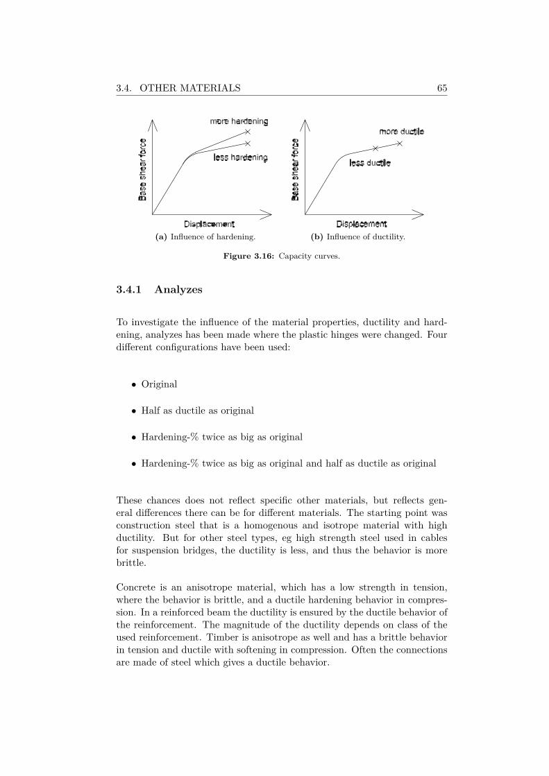
3.4. OTHER MATERIALS 65
(a) Influence of hardening. (b) Influence of ductility.
Figure 3.16: Capacity curves.
3.4.1 Analyzes
To investigate the influence of the material properties, ductility and hard-ening, analyzes has been made where the plastic hinges were changed. Fourdifferent configurations have been used:
• Original
• Half as ductile as original
• Hardening-% twice as big as original
• Hardening-% twice as big as original and half as ductile as original
These chances does not reflect specific other materials, but reflects gen-eral differences there can be for different materials. The starting point wasconstruction steel that is a homogenous and isotrope material with highductility. But for other steel types, eg high strength steel used in cablesfor suspension bridges, the ductility is less, and thus the behavior is morebrittle.
Concrete is an anisotrope material, which has a low strength in tension,where the behavior is brittle, and a ductile hardening behavior in compres-sion. In a reinforced beam the ductility is ensured by the ductile behavior ofthe reinforcement. The magnitude of the ductility depends on class of theused reinforcement. Timber is anisotrope as well and has a brittle behaviorin tension and ductile with softening in compression. Often the connectionsare made of steel which gives a ductile behavior.
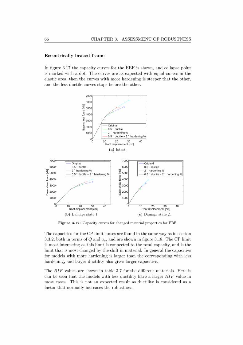
66 CHAPTER 3. ASSESSMENT OF ROBUSTNESS
Eccentrically braced frame
In figure 3.17 the capacity curves for the EBF is shown, and collapse pointis marked with a dot. The curves are as expected with equal curves in theelastic area, then the curves with more hardening is steeper that the other,and the less ductile curves stops before the other.
0 10 20 30 400
1000
2000
3000
4000
5000
6000
7000
Roof displacement [cm]
Bas
e sh
ear
forc
e [k
N]
Original0.5 ´ ductile2 ´ hardening %0.5 ´ ductile − 2 ´ hardening %
(a) Intact.
0 10 20 30 400
1000
2000
3000
4000
5000
6000
7000
Roof displacement [cm]
Bas
e sh
ear
forc
e [k
N]
Original0.5 ´ ductile2 ´ hardening %0.5 ´ ductile − 2 ´ hardening %
(b) Damage state 1.
0 10 20 30 400
1000
2000
3000
4000
5000
6000
7000
Roof displacement [cm]
Bas
e sh
ear
forc
e [k
N]
Original0.5 ´ ductile2 ´ hardening %0.5 ´ ductile − 2 ´ hardening %
(c) Damage state 2.
Figure 3.17: Capacity curves for changed material properties for EBF.
The capacities for the CP limit states are found in the same way as in section3.3.2, both in terms of Q and ag, and are shown in figure 3.18. The CP limitis most interesting as this limit is connected to the total capacity, and is thelimit that is most changed by the shift in material. In general the capacitiesfor models with more hardening is larger than the corresponding with lesshardening, and larger ductility also gives larger capacities.
The RIF values are shown in table 3.7 for the different materials. Here itcan be seen that the models with less ductility have a larger RIF value inmost cases. This is not an expected result as ductility is considered as afactor that normally increases the robustness.
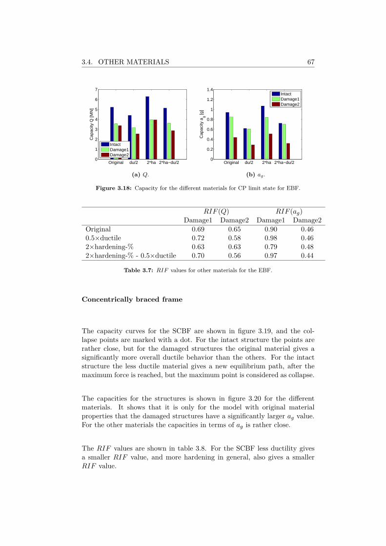
3.4. OTHER MATERIALS 67
Original du/2 2*ha 2*ha−du/20
1
2
3
4
5
6
7C
apac
ity Q
[MN
]
IntactDamage1Damage2
(a) Q.
Original du/2 2*ha 2*ha−du/20
0.2
0.4
0.6
0.8
1
1.2
1.4
Cap
acity
ag [g
]
IntactDamage1Damage2
(b) ag.
Figure 3.18: Capacity for the different materials for CP limit state for EBF.
RIF (Q) RIF (ag)Damage1 Damage2 Damage1 Damage2
Original 0.69 0.65 0.90 0.460.5×ductile 0.72 0.58 0.98 0.462×hardening-% 0.63 0.63 0.79 0.482×hardening-% - 0.5×ductile 0.70 0.56 0.97 0.44
Table 3.7: RIF values for other materials for the EBF.
Concentrically braced frame
The capacity curves for the SCBF are shown in figure 3.19, and the col-lapse points are marked with a dot. For the intact structure the points arerather close, but for the damaged structures the original material gives asignificantly more overall ductile behavior than the others. For the intactstructure the less ductile material gives a new equilibrium path, after themaximum force is reached, but the maximum point is considered as collapse.
The capacities for the structures is shown in figure 3.20 for the differentmaterials. It shows that it is only for the model with original materialproperties that the damaged structures have a significantly larger ag value.For the other materials the capacities in terms of ag is rather close.
The RIF values are shown in table 3.8. For the SCBF less ductility givesa smaller RIF value, and more hardening in general, also gives a smallerRIF value.
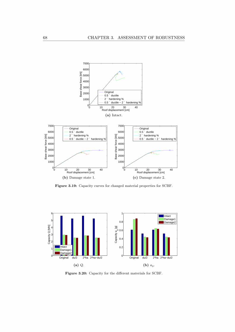
68 CHAPTER 3. ASSESSMENT OF ROBUSTNESS
0 10 20 30 400
1000
2000
3000
4000
5000
6000
7000
Roof displacement [cm]
Bas
e sh
ear
forc
e [k
N]
Original0.5 ´ ductile2 ´ hardening %0.5 ´ ductile − 2 ´ hardening %
(a) Intact.
0 10 20 30 400
1000
2000
3000
4000
5000
6000
7000
Roof displacement [cm]
Bas
e sh
ear
forc
e [k
N]
Original0.5 ´ ductile2 ´ hardening %0.5 ´ ductile − 2 ´ hardening %
(b) Damage state 1.
0 10 20 30 400
1000
2000
3000
4000
5000
6000
7000
Roof displacement [cm]
Bas
e sh
ear
forc
e [k
N]
Original0.5 ´ ductile2 ´ hardening %0.5 ´ ductile − 2 ´ hardening %
(c) Damage state 2.
Figure 3.19: Capacity curves for changed material properties for SCBF.
Original du/2 2*ha 2*ha−du/20
1
2
3
4
5
6
Cap
acity
Q [M
N]
IntactDamage1Damage2
(a) Q.
Original du/2 2*ha 2*ha−du/20
0.2
0.4
0.6
0.8
1
Cap
acity
ag [g
]
IntactDamage1Damage2
(b) ag.
Figure 3.20: Capacity for the different materials for SCBF.
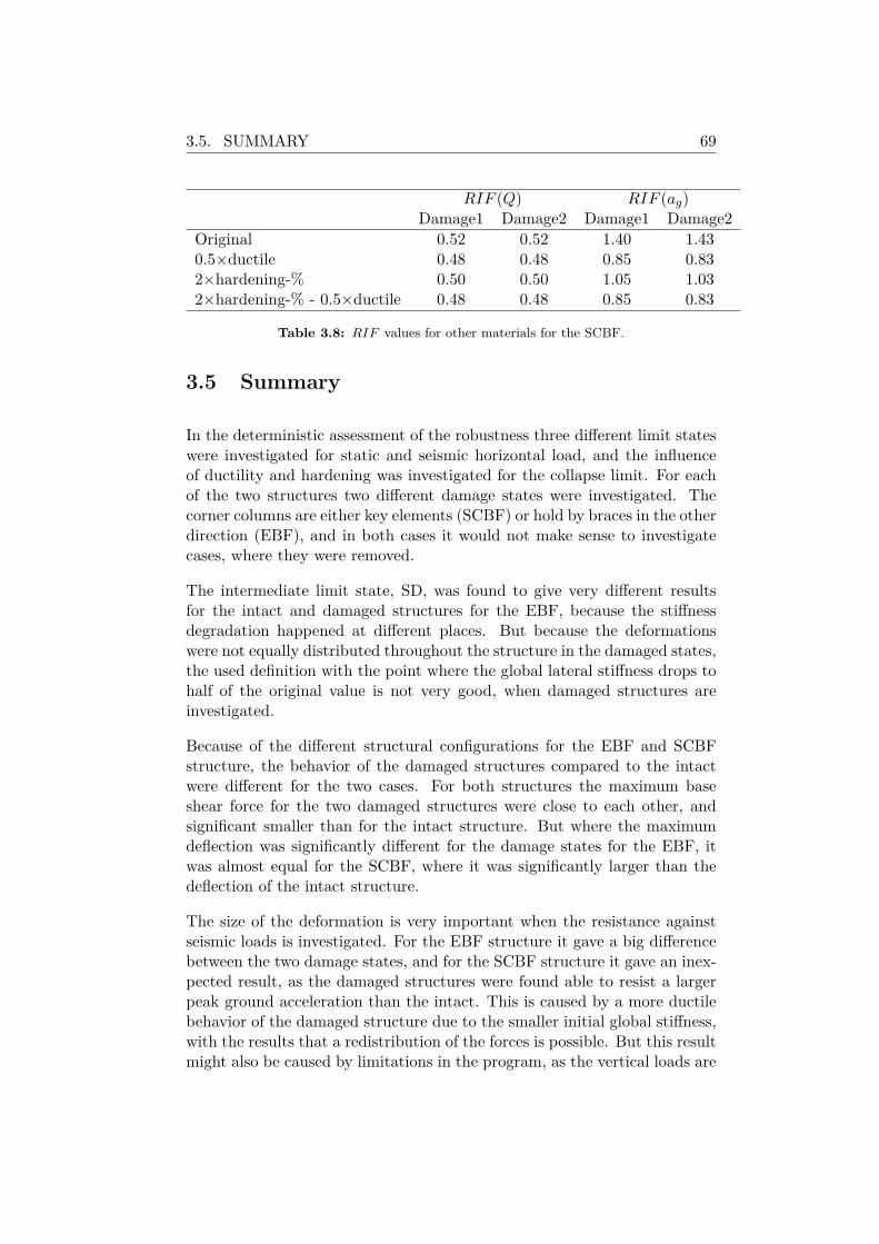
3.5. SUMMARY 69
RIF (Q) RIF (ag)Damage1 Damage2 Damage1 Damage2
Original 0.52 0.52 1.40 1.430.5×ductile 0.48 0.48 0.85 0.832×hardening-% 0.50 0.50 1.05 1.032×hardening-% - 0.5×ductile 0.48 0.48 0.85 0.83
Table 3.8: RIF values for other materials for the SCBF.
3.5 Summary
In the deterministic assessment of the robustness three different limit stateswere investigated for static and seismic horizontal load, and the influenceof ductility and hardening was investigated for the collapse limit. For eachof the two structures two different damage states were investigated. Thecorner columns are either key elements (SCBF) or hold by braces in the otherdirection (EBF), and in both cases it would not make sense to investigatecases, where they were removed.
The intermediate limit state, SD, was found to give very different resultsfor the intact and damaged structures for the EBF, because the stiffnessdegradation happened at different places. But because the deformationswere not equally distributed throughout the structure in the damaged states,the used definition with the point where the global lateral stiffness drops tohalf of the original value is not very good, when damaged structures areinvestigated.
Because of the different structural configurations for the EBF and SCBFstructure, the behavior of the damaged structures compared to the intactwere different for the two cases. For both structures the maximum baseshear force for the two damaged structures were close to each other, andsignificant smaller than for the intact structure. But where the maximumdeflection was significantly different for the damage states for the EBF, itwas almost equal for the SCBF, where it was significantly larger than thedeflection of the intact structure.
The size of the deformation is very important when the resistance againstseismic loads is investigated. For the EBF structure it gave a big differencebetween the two damage states, and for the SCBF structure it gave an inex-pected result, as the damaged structures were found able to resist a largerpeak ground acceleration than the intact. This is caused by a more ductilebehavior of the damaged structure due to the smaller initial global stiffness,with the results that a redistribution of the forces is possible. But this resultmight also be caused by limitations in the program, as the vertical loads are
70 CHAPTER 3. ASSESSMENT OF ROBUSTNESS
not taken into account, and the intact structure might still have additionalcapacity left at the point defined as collapse. The use of more complicatedanalysis methods might give another result, and also the use of a spatialmodel instead of a plane model would make it possible to take torsional ef-fects into account. But in principle it is possible for a damaged structure toact more ductile, and thereby perform better during an earthquake, yieldinga RIF value of more than one.
The ductility is a parameter that is normally considered as important for therobustness when the alternate load path strategy is used. The analyzes withdifferent ductility and hardening showed that the structures with more duc-tile behavior were in fact able to resist a larger force and ground accelerationthan those with smaller ductility. But when the RIF value is calculated amore ductile behavior both makes the intact and damaged structures per-form better, and in fact it was found to increase the capacity more for theintact than for the damaged structures, yielding that more ductility gives asmaller RIF value, with the used definition. This means that if earthquakeresistant structures are designed taking the actual ductility into account, astructure with less ductile behavior would have a higher seismic resistancein a damaged case.
In general increased hardening was found to give larger capacities, exceptfor damaged states for the SCBF. Here the hardening seems to restrict thedeformations, giving less ductile behavior, and thus a smaller capacity interms of peak ground acceleration.
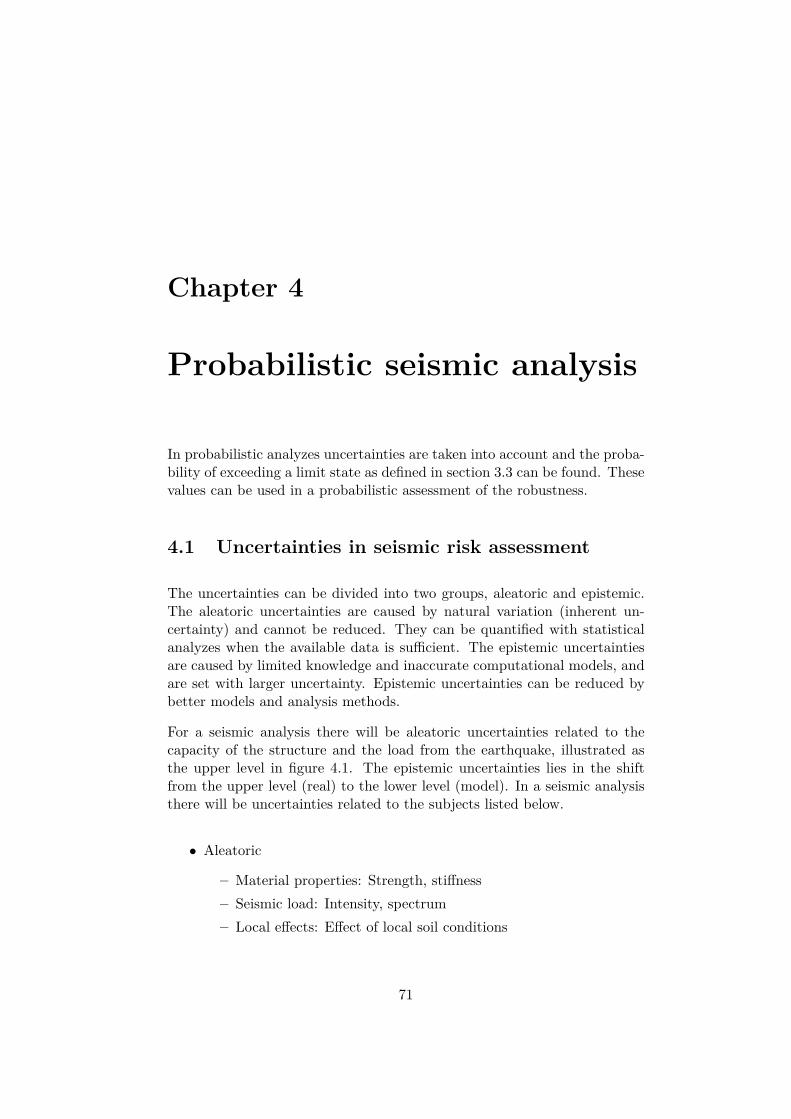
Chapter 4
Probabilistic seismic analysis
In probabilistic analyzes uncertainties are taken into account and the proba-bility of exceeding a limit state as defined in section 3.3 can be found. Thesevalues can be used in a probabilistic assessment of the robustness.
4.1 Uncertainties in seismic risk assessment
The uncertainties can be divided into two groups, aleatoric and epistemic.The aleatoric uncertainties are caused by natural variation (inherent un-certainty) and cannot be reduced. They can be quantified with statisticalanalyzes when the available data is sufficient. The epistemic uncertaintiesare caused by limited knowledge and inaccurate computational models, andare set with larger uncertainty. Epistemic uncertainties can be reduced bybetter models and analysis methods.
For a seismic analysis there will be aleatoric uncertainties related to thecapacity of the structure and the load from the earthquake, illustrated asthe upper level in figure 4.1. The epistemic uncertainties lies in the shiftfrom the upper level (real) to the lower level (model). In a seismic analysisthere will be uncertainties related to the subjects listed below.
• Aleatoric
– Material properties: Strength, stiffness– Seismic load: Intensity, spectrum– Local effects: Effect of local soil conditions
71
72 CHAPTER 4. PROBABILISTIC SEISMIC ANALYSIS
Figure 4.1: Uncertainties in seismic risk assessment.
• Epistemic
– Model of structure: Connections, panel zones, inelastic behavior,plane vs. spatial, mass distribution
– Analysis of structural model: Time history analysis (dynamic)vs. static analysis with equal effective damping
– Model of earthquake: Time history→ general response spectrum– Failure functions: Definition of limit states
4.2 Procedure for seismic risk assessment
A procedure for assessing the annual probability of exceeding a limit statewas proposed by [Ellingwood & Kinali 2009].
The limit state probability, PLS, in seismic risk assessment is defined as:
PLS =∑x
P [Sa = x] · P [LS|Sa = x] (4.1)
where Sa is the intensity measured in terms of the peak spectral accelerationat the period of the structure, P [Sa = x] is the probability that the intensityof the seismic demand is x, and P [LS|Sa = x] is the probability of exceeding adefined limit state given that Sa = x. In this way the problem is divided intotwo quantities, the first dependent on the seismic demand and the seconddependent on the capacity of the structure. [Ellingwood & Kinali 2009]
4.2. PROCEDURE FOR SEISMIC RISK ASSESSMENT 73
4.2.1 Capacity
The failure function can be written as:
g = MR −X (4.2)
whereMR is the capacity in terms of Sa and X is the seismic demand (load)in terms of Sa. If both are considered as lognormal distributed stochasticvariables the failure function can equivalently be expressed as:
g = ln(MR)− ln(X) (4.3)
Using the definition of the reliability index, β, the probability of exceedinga given limit state can for a specific Sa be calculated as:
P [LS|Sa = x] = Φ(−β) = Φ(− ln(mR)− ln(x)
σR
)= Φ
( ln(x/mR)σR
)(4.4)
wheremR and σR is the median value and the logarithmic standard deviationof the capacity respectively, and x is the given demand.
As described in section 3.3.2 the limit states can be expressed as limit valuesof ISDA, and thus the capacity in terms of Sa can be transmitted into acapacity in terms of ISDA. This can be done using the relationship:
mc = a ·mRb (4.5)
where mc is the capacity in terms of ISDA and a and b are regression con-stants. In [Ellingwood & Kinali 2009] this relationship was found using timehistory analyzes with a range of different earthquake records as input. As iscan be seen in figure 4.2 there are uncertainty connected with this model, asthe found points are not located at a perfect curve, and the logarithmic stan-dard deviation connected with the relationship is called σD|Sa (drift (ISDA)given Sa). In [Ellingwood & Kinali 2009] this is referred to as aleatoric un-certainty, because it is caused by the structures different behavior towardsthe natural difference in earthquakes. But it it also connected to the modelgiving the relationship between the ISDA and Sa, which is an argumentthat is should be counted as epistemic uncertainty, but in [Ellingwood &Kinali 2009] it is assumed that the deviance from the curve is caused byaleatoric uncertainty alone. The epistemic uncertainty connected to themodel and the time history analyzes is called σRU .
Insertion of equation 4.5 into 4.4 gives the following expression for the prob-ability of exceeding a given limit state given Sa = x.
P [LS|Sa = x] = Φ(
ln(axb/mc)σR
)(4.6)
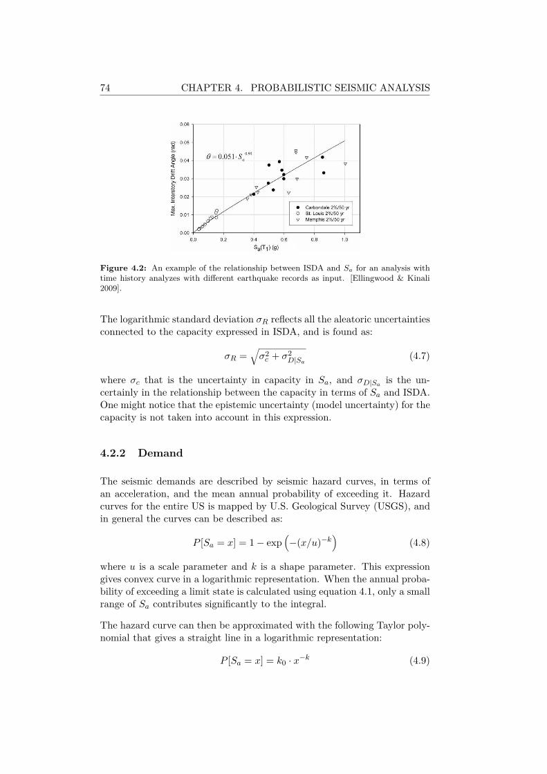
74 CHAPTER 4. PROBABILISTIC SEISMIC ANALYSIS
Figure 4.2: An example of the relationship between ISDA and Sa for an analysis withtime history analyzes with different earthquake records as input. [Ellingwood & Kinali2009].
The logarithmic standard deviation σR reflects all the aleatoric uncertaintiesconnected to the capacity expressed in ISDA, and is found as:
σR =√σ2c + σ2
D|Sa (4.7)
where σc that is the uncertainty in capacity in Sa, and σD|Sa is the un-certainly in the relationship between the capacity in terms of Sa and ISDA.One might notice that the epistemic uncertainty (model uncertainty) for thecapacity is not taken into account in this expression.
4.2.2 Demand
The seismic demands are described by seismic hazard curves, in terms ofan acceleration, and the mean annual probability of exceeding it. Hazardcurves for the entire US is mapped by U.S. Geological Survey (USGS), andin general the curves can be described as:
P [Sa = x] = 1− exp(−(x/u)−k
)(4.8)
where u is a scale parameter and k is a shape parameter. This expressiongives convex curve in a logarithmic representation. When the annual proba-bility of exceeding a limit state is calculated using equation 4.1, only a smallrange of Sa contributes significantly to the integral.
The hazard curve can then be approximated with the following Taylor poly-nomial that gives a straight line in a logarithmic representation:
P [Sa = x] = k0 · x−k (4.9)
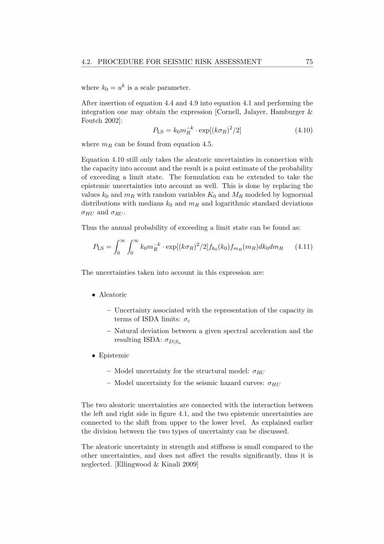
4.2. PROCEDURE FOR SEISMIC RISK ASSESSMENT 75
where k0 = uk is a scale parameter.
After insertion of equation 4.4 and 4.9 into equation 4.1 and performing theintegration one may obtain the expression [Cornell, Jalayer, Hamburger &Foutch 2002]:
PLS = k0m−kR · exp[(kσR)2/2] (4.10)
where mR can be found from equation 4.5.
Equation 4.10 still only takes the aleatoric uncertainties in connection withthe capacity into account and the result is a point estimate of the probabilityof exceeding a limit state. The formulation can be extended to take theepistemic uncertainties into account as well. This is done by replacing thevalues k0 and mR with random variables K0 and MR modeled by lognormaldistributions with medians k0 and mR and logarithmic standard deviationsσHU and σRU .
Thus the annual probability of exceeding a limit state can be found as:
PLS =∫ ∞
0
∫ ∞0
k0m−kR · exp[(kσR)2/2]fk0(k0)fmR(mR)dk0dmR (4.11)
The uncertainties taken into account in this expression are:
• Aleatoric
– Uncertainty associated with the representation of the capacity interms of ISDA limits: σc
– Natural deviation between a given spectral acceleration and theresulting ISDA: σD|Sa
• Epistemic
– Model uncertainty for the structural model: σRU– Model uncertainty for the seismic hazard curves: σHU
The two aleatoric uncertainties are connected with the interaction betweenthe left and right side in figure 4.1, and the two epistemic uncertainties areconnected to the shift from upper to the lower level. As explained earlierthe division between the two types of uncertainty can be discussed.
The aleatoric uncertainty in strength and stiffness is small compared to theother uncertainties, and does not affect the results significantly, thus it isneglected. [Ellingwood & Kinali 2009]
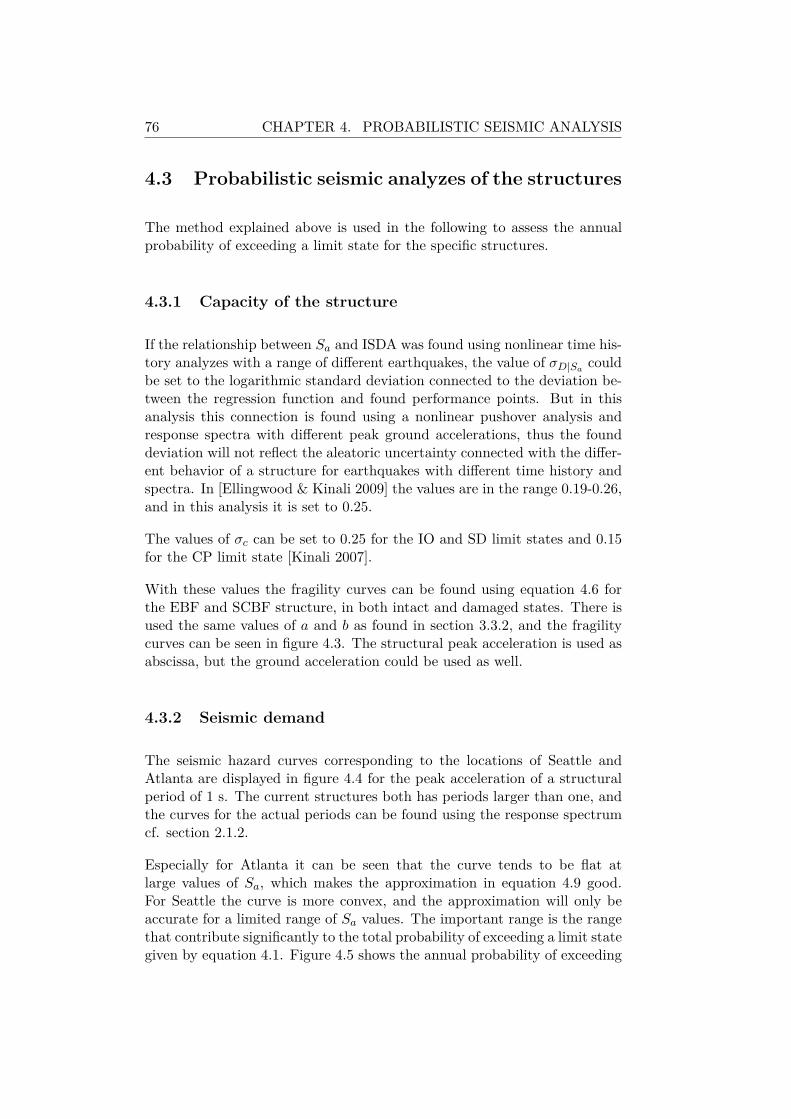
76 CHAPTER 4. PROBABILISTIC SEISMIC ANALYSIS
4.3 Probabilistic seismic analyzes of the structures
The method explained above is used in the following to assess the annualprobability of exceeding a limit state for the specific structures.
4.3.1 Capacity of the structure
If the relationship between Sa and ISDA was found using nonlinear time his-tory analyzes with a range of different earthquakes, the value of σD|Sa couldbe set to the logarithmic standard deviation connected to the deviation be-tween the regression function and found performance points. But in thisanalysis this connection is found using a nonlinear pushover analysis andresponse spectra with different peak ground accelerations, thus the founddeviation will not reflect the aleatoric uncertainty connected with the differ-ent behavior of a structure for earthquakes with different time history andspectra. In [Ellingwood & Kinali 2009] the values are in the range 0.19-0.26,and in this analysis it is set to 0.25.
The values of σc can be set to 0.25 for the IO and SD limit states and 0.15for the CP limit state [Kinali 2007].
With these values the fragility curves can be found using equation 4.6 forthe EBF and SCBF structure, in both intact and damaged states. There isused the same values of a and b as found in section 3.3.2, and the fragilitycurves can be seen in figure 4.3. The structural peak acceleration is used asabscissa, but the ground acceleration could be used as well.
4.3.2 Seismic demand
The seismic hazard curves corresponding to the locations of Seattle andAtlanta are displayed in figure 4.4 for the peak acceleration of a structuralperiod of 1 s. The current structures both has periods larger than one, andthe curves for the actual periods can be found using the response spectrumcf. section 2.1.2.
Especially for Atlanta it can be seen that the curve tends to be flat atlarge values of Sa, which makes the approximation in equation 4.9 good.For Seattle the curve is more convex, and the approximation will only beaccurate for a limited range of Sa values. The important range is the rangethat contribute significantly to the total probability of exceeding a limit stategiven by equation 4.1. Figure 4.5 shows the annual probability of exceeding
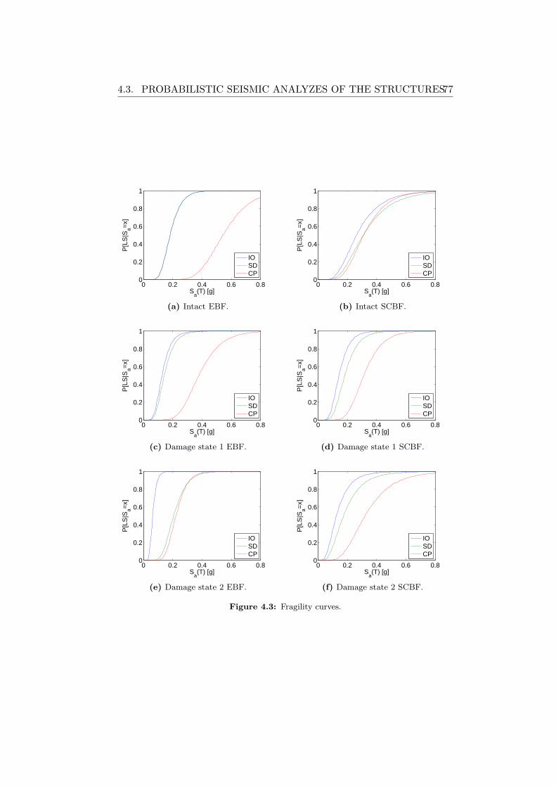
4.3. PROBABILISTIC SEISMIC ANALYZES OF THE STRUCTURES77
0 0.2 0.4 0.6 0.80
0.2
0.4
0.6
0.8
1
Sa(T) [g]
P[L
S|S
a=x]
IOSDCP
(a) Intact EBF.
0 0.2 0.4 0.6 0.80
0.2
0.4
0.6
0.8
1
Sa(T) [g]
P[L
S|S
a=x]
IOSDCP
(b) Intact SCBF.
0 0.2 0.4 0.6 0.80
0.2
0.4
0.6
0.8
1
Sa(T) [g]
P[L
S|S
a=x]
IOSDCP
(c) Damage state 1 EBF.
0 0.2 0.4 0.6 0.80
0.2
0.4
0.6
0.8
1
Sa(T) [g]
P[L
S|S
a=x]
IOSDCP
(d) Damage state 1 SCBF.
0 0.2 0.4 0.6 0.80
0.2
0.4
0.6
0.8
1
Sa(T) [g]
P[L
S|S
a=x]
IOSDCP
(e) Damage state 2 EBF.
0 0.2 0.4 0.6 0.80
0.2
0.4
0.6
0.8
1
Sa(T) [g]
P[L
S|S
a=x]
IOSDCP
(f) Damage state 2 SCBF.
Figure 4.3: Fragility curves.
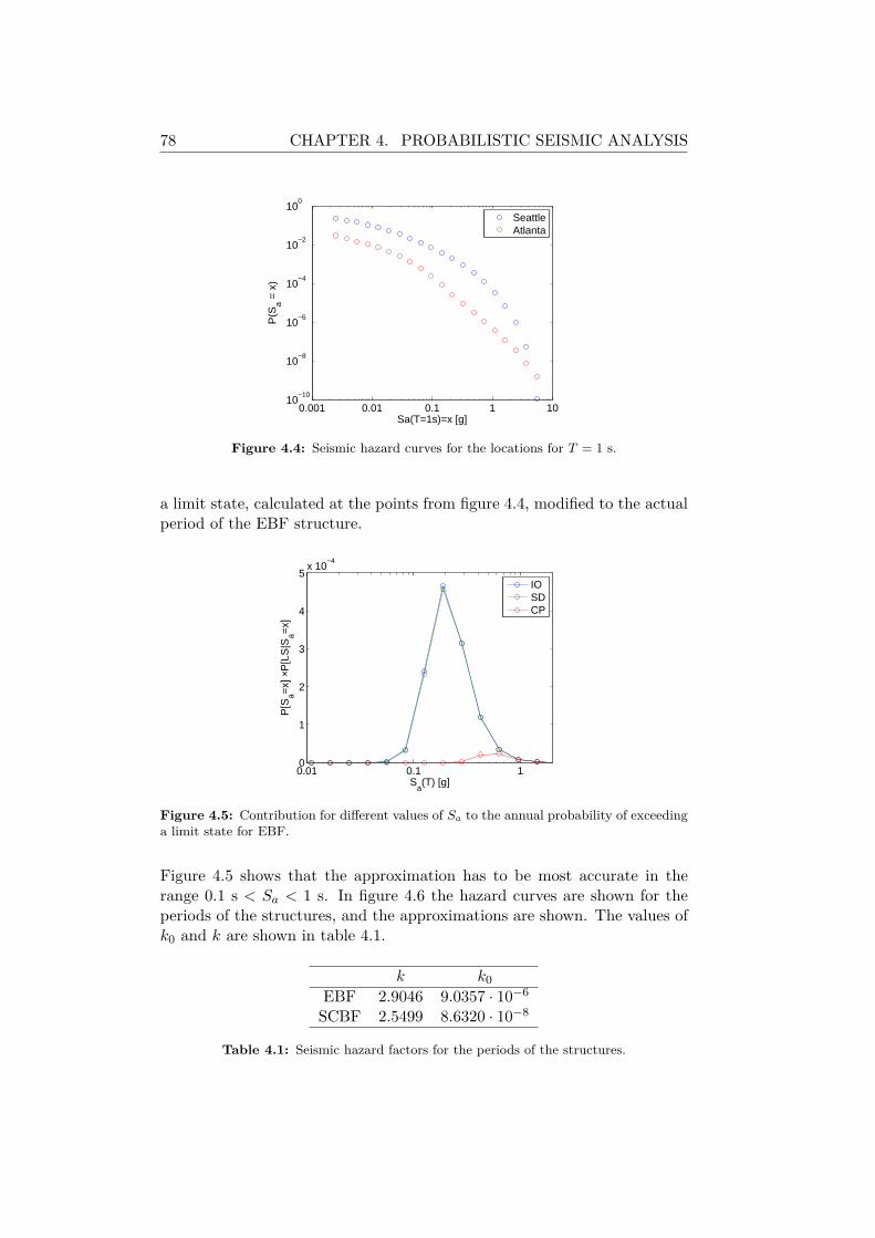
78 CHAPTER 4. PROBABILISTIC SEISMIC ANALYSIS
0.001 0.01 0.1 1 1010
−10
10−8
10−6
10−4
10−2
100
Sa(T=1s)=x [g]
P(S
a = x
)
SeattleAtlanta
Figure 4.4: Seismic hazard curves for the locations for T = 1 s.
a limit state, calculated at the points from figure 4.4, modified to the actualperiod of the EBF structure.
0.01 0.1 10
1
2
3
4
5x 10
−4
Sa(T) [g]
P[S
a=x]
× P
[LS
|Sa=
x]
IOSDCP
Figure 4.5: Contribution for different values of Sa to the annual probability of exceedinga limit state for EBF.
Figure 4.5 shows that the approximation has to be most accurate in therange 0.1 s < Sa < 1 s. In figure 4.6 the hazard curves are shown for theperiods of the structures, and the approximations are shown. The values ofk0 and k are shown in table 4.1.
k k0EBF 2.9046 9.0357 · 10−6
SCBF 2.5499 8.6320 · 10−8
Table 4.1: Seismic hazard factors for the periods of the structures.
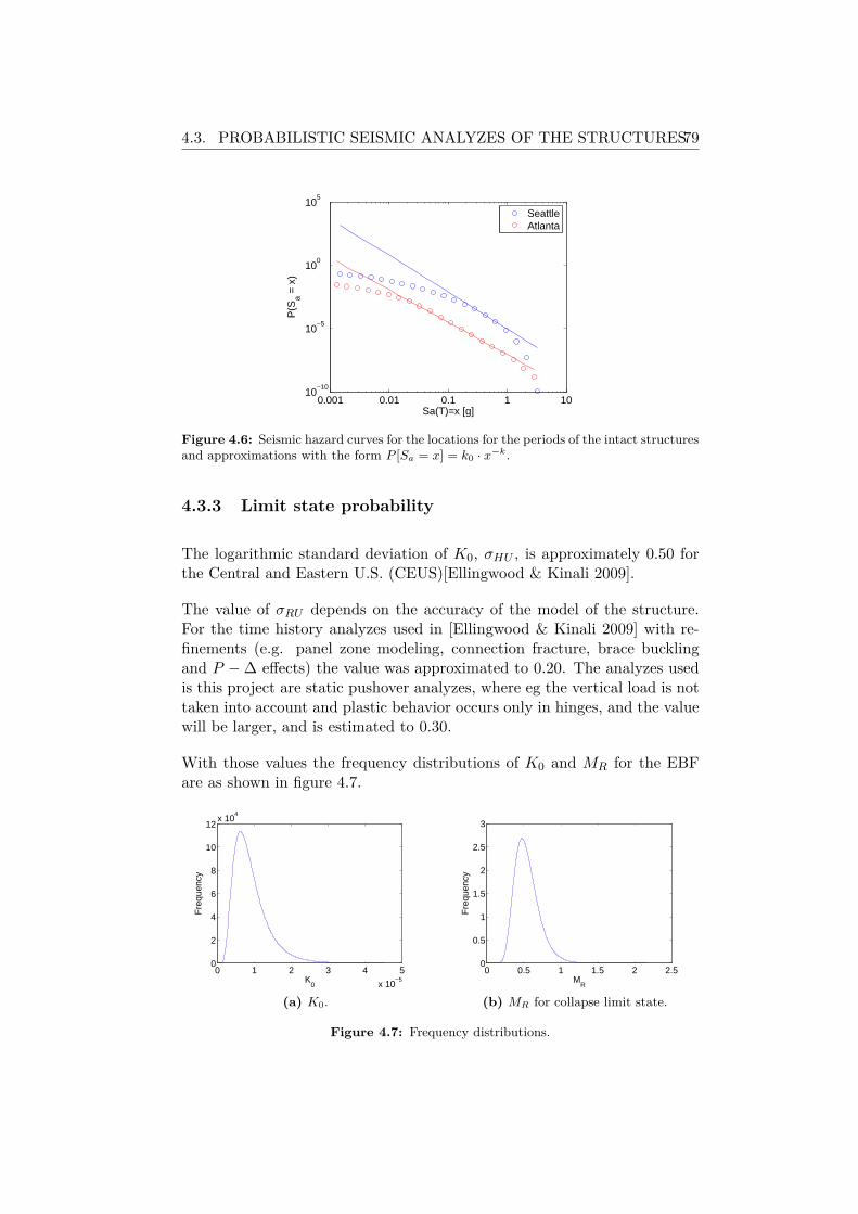
4.3. PROBABILISTIC SEISMIC ANALYZES OF THE STRUCTURES79
0.001 0.01 0.1 1 1010
−10
10−5
100
105
Sa(T)=x [g]
P(S
a = x
)
SeattleAtlanta
Figure 4.6: Seismic hazard curves for the locations for the periods of the intact structuresand approximations with the form P [Sa = x] = k0 · x−k.
4.3.3 Limit state probability
The logarithmic standard deviation of K0, σHU , is approximately 0.50 forthe Central and Eastern U.S. (CEUS)[Ellingwood & Kinali 2009].
The value of σRU depends on the accuracy of the model of the structure.For the time history analyzes used in [Ellingwood & Kinali 2009] with re-finements (e.g. panel zone modeling, connection fracture, brace bucklingand P −∆ effects) the value was approximated to 0.20. The analyzes usedis this project are static pushover analyzes, where eg the vertical load is nottaken into account and plastic behavior occurs only in hinges, and the valuewill be larger, and is estimated to 0.30.
With those values the frequency distributions of K0 and MR for the EBFare as shown in figure 4.7.
0 1 2 3 4 5
x 10−5
0
2
4
6
8
10
12x 10
4
K0
Fre
quen
cy
(a) K0.
0 0.5 1 1.5 2 2.50
0.5
1
1.5
2
2.5
3
Fre
quen
cy
MR
(b) MR for collapse limit state.
Figure 4.7: Frequency distributions.
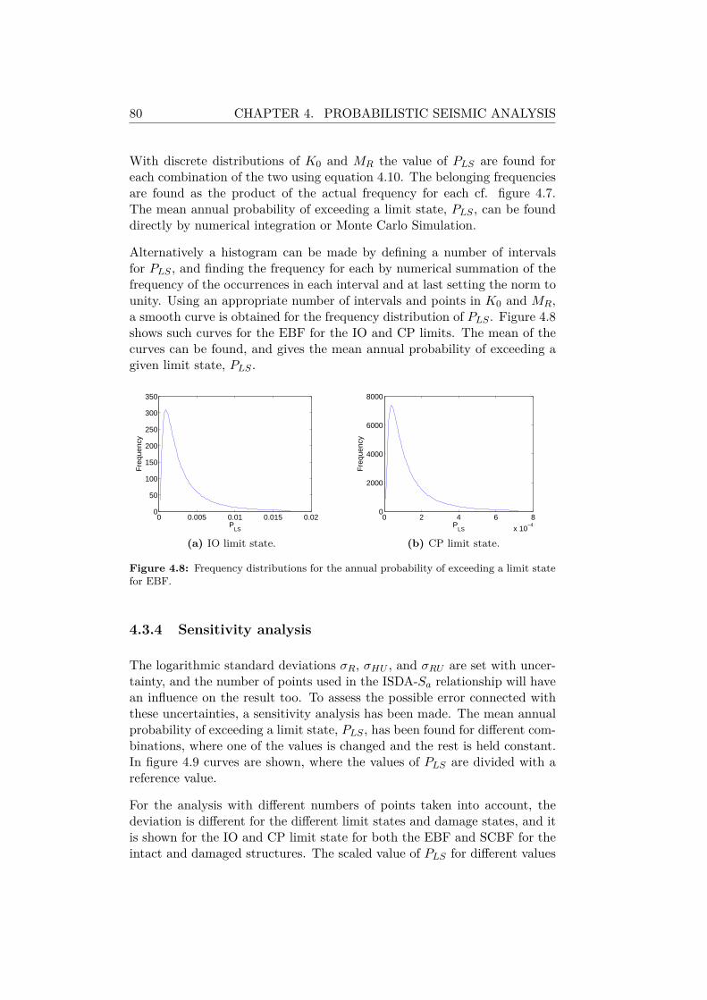
80 CHAPTER 4. PROBABILISTIC SEISMIC ANALYSIS
With discrete distributions of K0 and MR the value of PLS are found foreach combination of the two using equation 4.10. The belonging frequenciesare found as the product of the actual frequency for each cf. figure 4.7.The mean annual probability of exceeding a limit state, PLS , can be founddirectly by numerical integration or Monte Carlo Simulation.
Alternatively a histogram can be made by defining a number of intervalsfor PLS , and finding the frequency for each by numerical summation of thefrequency of the occurrences in each interval and at last setting the norm tounity. Using an appropriate number of intervals and points in K0 and MR,a smooth curve is obtained for the frequency distribution of PLS . Figure 4.8shows such curves for the EBF for the IO and CP limits. The mean of thecurves can be found, and gives the mean annual probability of exceeding agiven limit state, PLS .
0 0.005 0.01 0.015 0.020
50
100
150
200
250
300
350
PLS
Fre
quen
cy
(a) IO limit state.
0 2 4 6 8
x 10−4
0
2000
4000
6000
8000
PLS
Fre
quen
cy
(b) CP limit state.
Figure 4.8: Frequency distributions for the annual probability of exceeding a limit statefor EBF.
4.3.4 Sensitivity analysis
The logarithmic standard deviations σR, σHU , and σRU are set with uncer-tainty, and the number of points used in the ISDA-Sa relationship will havean influence on the result too. To assess the possible error connected withthese uncertainties, a sensitivity analysis has been made. The mean annualprobability of exceeding a limit state, PLS , has been found for different com-binations, where one of the values is changed and the rest is held constant.In figure 4.9 curves are shown, where the values of PLS are divided with areference value.
For the analysis with different numbers of points taken into account, thedeviation is different for the different limit states and damage states, and itis shown for the IO and CP limit state for both the EBF and SCBF for theintact and damaged structures. The scaled value of PLS for different values
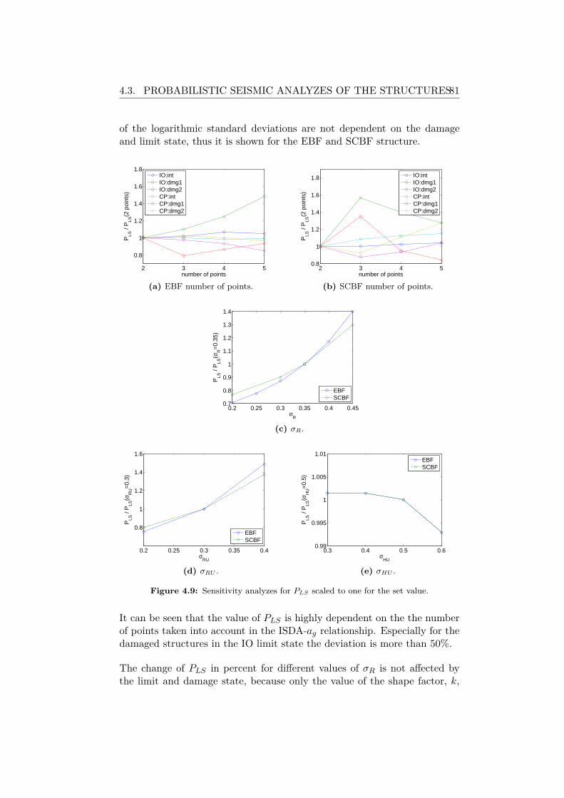
4.3. PROBABILISTIC SEISMIC ANALYZES OF THE STRUCTURES81
of the logarithmic standard deviations are not dependent on the damageand limit state, thus it is shown for the EBF and SCBF structure.
2 3 4 5
0.8
1
1.2
1.4
1.6
1.8
number of points
PLS
/ P
LS(2
poi
nts)
IO:intIO:dmg1IO:dmg2CP:intCP:dmg1CP:dmg2
(a) EBF number of points.
2 3 4 50.8
1
1.2
1.4
1.6
1.8
number of points
PLS
/ P
LS(2
poi
nts)
IO:intIO:dmg1IO:dmg2CP:intCP:dmg1CP:dmg2
(b) SCBF number of points.
0.2 0.25 0.3 0.35 0.4 0.450.7
0.8
0.9
1
1.1
1.2
1.3
1.4
σR
PLS
/ P
LS(σ
R=
0.35
)
EBFSCBF
(c) σR.
0.2 0.25 0.3 0.35 0.4
0.8
1
1.2
1.4
1.6
σRU
PLS
/ P
LS(σ
RU=
0.3)
EBFSCBF
(d) σRU .
0.3 0.4 0.5 0.60.99
0.995
1
1.005
1.01
σHU
PLS
/ P
LS(σ
HU=
0.5)
EBFSCBF
(e) σHU .
Figure 4.9: Sensitivity analyzes for PLS scaled to one for the set value.
It can be seen that the value of PLS is highly dependent on the the numberof points taken into account in the ISDA-ag relationship. Especially for thedamaged structures in the IO limit state the deviation is more than 50%.
The change of PLS in percent for different values of σR is not affected bythe limit and damage state, because only the value of the shape factor, k,
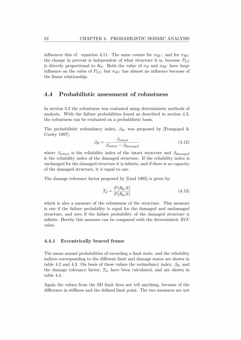
82 CHAPTER 4. PROBABILISTIC SEISMIC ANALYSIS
influences this cf. equation 4.11. The same counts for σRU , and for σHUthe change in percent is independent of what structure it is, because PLSis directly proportional to K0. Both the value of σR and σRU have largeinfluence on the value of PLS , but σHU has almost no influence because ofthe linear relationship.
4.4 Probabilistic assessment of robustness
In section 3.3 the robustness was evaluated using deterministic methods ofanalysis. With the failure probabilities found as described in section 4.3,the robustness can be evaluated on a probabilistic basis.
The probabilistic redundancy index, βR, was proposed by [Frangopol &Curley 1987]:
βR = βintactβintact − βdamaged (4.12)
where βintact is the reliability index of the intact structure and βdamagedis the reliability index of the damaged structure. If the reliability index isunchanged for the damaged structure it is infinite, and if there is no capacityof the damaged structure, it is equal to one.
The damage tolerance factor proposed by [Lind 1995] is given by:
Td = P (R0,S)P (Rd,S) (4.13)
which is also a measure of the robustness of the structure. This measureis one if the failure probability is equal for the damaged and undamagedstructure, and zero if the failure probability of the damaged structure isinfinite. Hereby this measure can be compared with the deterministic RIFvalue.
4.4.1 Eccentrically braced frame
The mean annual probabilities of exceeding a limit state, and the reliabilityindices corresponding to the different limit and damage states are shown intable 4.2 and 4.3. On basis of these values the redundancy index, βR, andthe damage tolerance factor, Td, have been calculated, and are shown intable 4.4.
Again the values from the SD limit does not tell anything, because of thedifference in stiffness and the defined limit point. The two measures are not
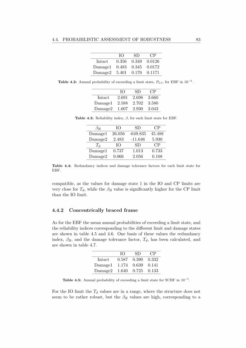
4.4. PROBABILISTIC ASSESSMENT OF ROBUSTNESS 83
IO SD CPIntact 0.356 0.349 0.0126
Damage1 0.483 0.345 0.0172Damage2 5.401 0.170 0.1171
Table 4.2: Annual probability of exceeding a limit state, PLS , for EBF in 10−2 .
IO SD CPIntact 2.691 2.698 3.660
Damage1 2.588 2.702 3.580Damage2 1.607 2.930 3.043
Table 4.3: Reliability index, β, for each limit state for EBF.
βR IO SD CPDamage1 26.056 -649.835 45.488Damage2 2.483 -11.646 5.930
Td IO SD CPDamage1 0.737 1.013 0.733Damage2 0.066 2.056 0.108
Table 4.4: Redundancy indices and damage tolerance factors for each limit state forEBF.
compatible, as the values for damage state 1 in the IO and CP limits arevery close for Td, while the βR value is significantly higher for the CP limitthan the IO limit.
4.4.2 Concentrically braced frame
As for the EBF the mean annual probabilities of exceeding a limit state, andthe reliability indices corresponding to the different limit and damage statesare shown in table 4.5 and 4.6. One basis of these values the redundancyindex, βR, and the damage tolerance factor, Td, has been calculated, andare shown in table 4.7.
IO SD CPIntact 0.587 0.390 0.332
Damage1 1.174 0.639 0.141Damage2 1.640 0.725 0.133
Table 4.5: Annual probability of exceeding a limit state for SCBF in 10−5.
For the IO limit the Td values are in a range, where the structure does notseem to be rather robust, but the βR values are high, corresponding to a
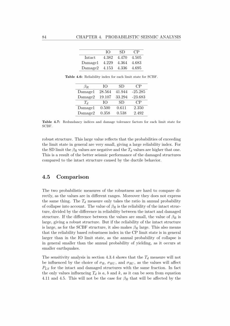
84 CHAPTER 4. PROBABILISTIC SEISMIC ANALYSIS
IO SD CPIntact 4.382 4.470 4.505
Damage1 4.229 4.364 4.683Damage2 4.153 4.336 4.695
Table 4.6: Reliability index for each limit state for SCBF.
βR IO SD CPDamage1 28.564 41.944 -25.285Damage2 19.107 33.294 -23.683
Td IO SD CPDamage1 0.500 0.611 2.350Damage2 0.358 0.538 2.492
Table 4.7: Redundancy indices and damage tolerance factors for each limit state forSCBF.
robust structure. This large value reflects that the probabilities of exceedingthe limit state in general are very small, giving a large reliability index. Forthe SD limit the βR values are negative and the Td values are higher that one.This is a result of the better seismic performance of the damaged structurescompared to the intact structure caused by the ductile behavior.
4.5 Comparison
The two probabilistic measures of the robustness are hard to compare di-rectly, as the values are in different ranges. Moreover they does not expressthe same thing. The Td measure only takes the ratio in annual probabilityof collapse into account. The value of βR is the reliability of the intact struc-ture, divided by the difference in reliability between the intact and damagedstructure. If the difference between the values are small, the value of βR islarge, giving a robust structure. But if the reliability of the intact structureis large, as for the SCBF structure, it also makes βR large. This also meansthat the reliability based robustness index in the CP limit state is in generallarger than in the IO limit state, as the annual probability of collapse isin general smaller than the annual probability of yielding, as it occurs atsmaller earthquakes.
The sensitivity analysis in section 4.3.4 shows that the Td measure will notbe influenced by the choice of σR, σHU , and σRU , as the values will affectPLS for the intact and damaged structures with the same fraction. In factthe only values influencing Td is a, b and k, as it can be seen from equation4.11 and 4.5. This will not be the case for βR that will be affected by the
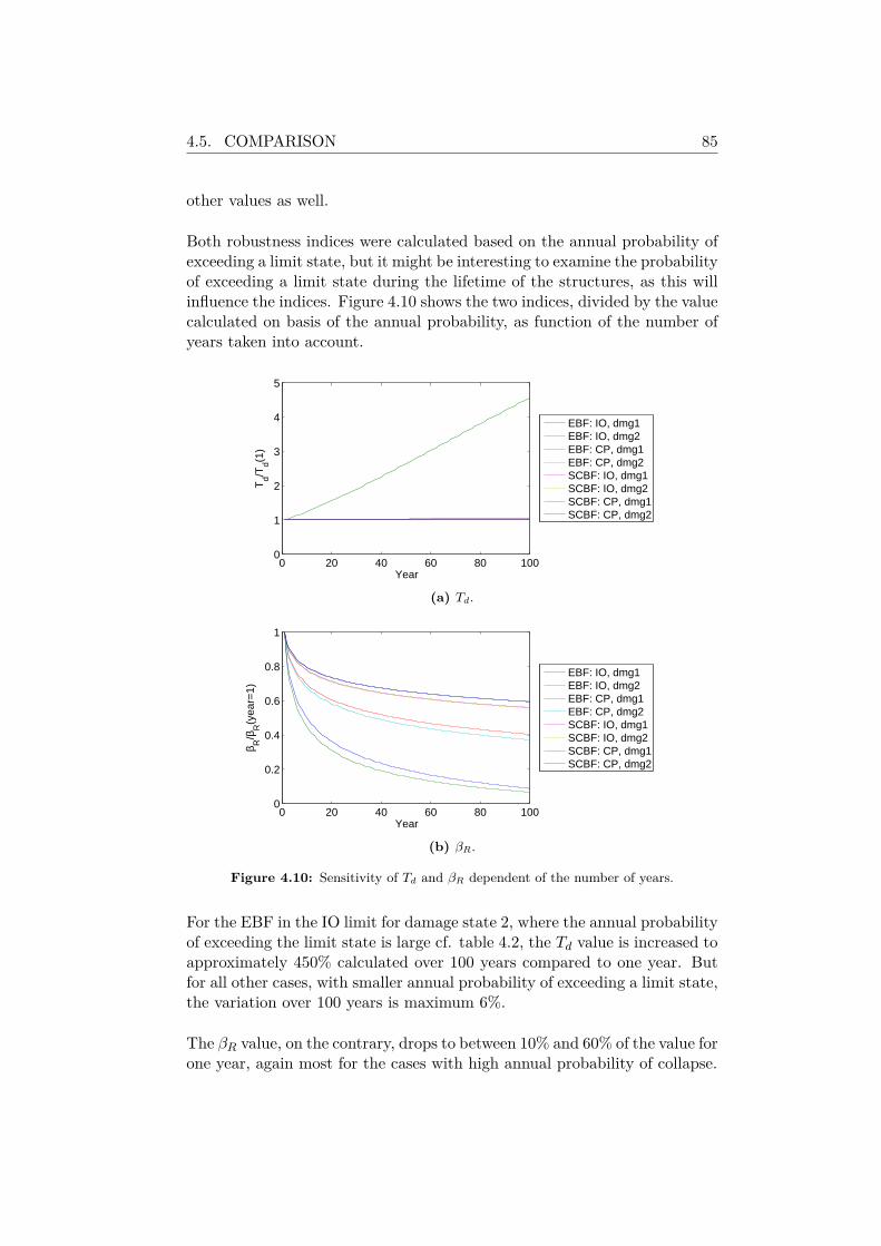
4.5. COMPARISON 85
other values as well.
Both robustness indices were calculated based on the annual probability ofexceeding a limit state, but it might be interesting to examine the probabilityof exceeding a limit state during the lifetime of the structures, as this willinfluence the indices. Figure 4.10 shows the two indices, divided by the valuecalculated on basis of the annual probability, as function of the number ofyears taken into account.
0 20 40 60 80 1000
1
2
3
4
5
Year
Td/T
d(1)
EBF: IO, dmg1EBF: IO, dmg2EBF: CP, dmg1EBF: CP, dmg2SCBF: IO, dmg1SCBF: IO, dmg2SCBF: CP, dmg1SCBF: CP, dmg2
(a) Td.
0 20 40 60 80 1000
0.2
0.4
0.6
0.8
1
Year
β R/β
R(y
ear=
1)
EBF: IO, dmg1EBF: IO, dmg2EBF: CP, dmg1EBF: CP, dmg2SCBF: IO, dmg1SCBF: IO, dmg2SCBF: CP, dmg1SCBF: CP, dmg2
(b) βR.
Figure 4.10: Sensitivity of Td and βR dependent of the number of years.
For the EBF in the IO limit for damage state 2, where the annual probabilityof exceeding the limit state is large cf. table 4.2, the Td value is increased toapproximately 450% calculated over 100 years compared to one year. Butfor all other cases, with smaller annual probability of exceeding a limit state,the variation over 100 years is maximum 6%.
The βR value, on the contrary, drops to between 10% and 60% of the value forone year, again most for the cases with high annual probability of collapse.
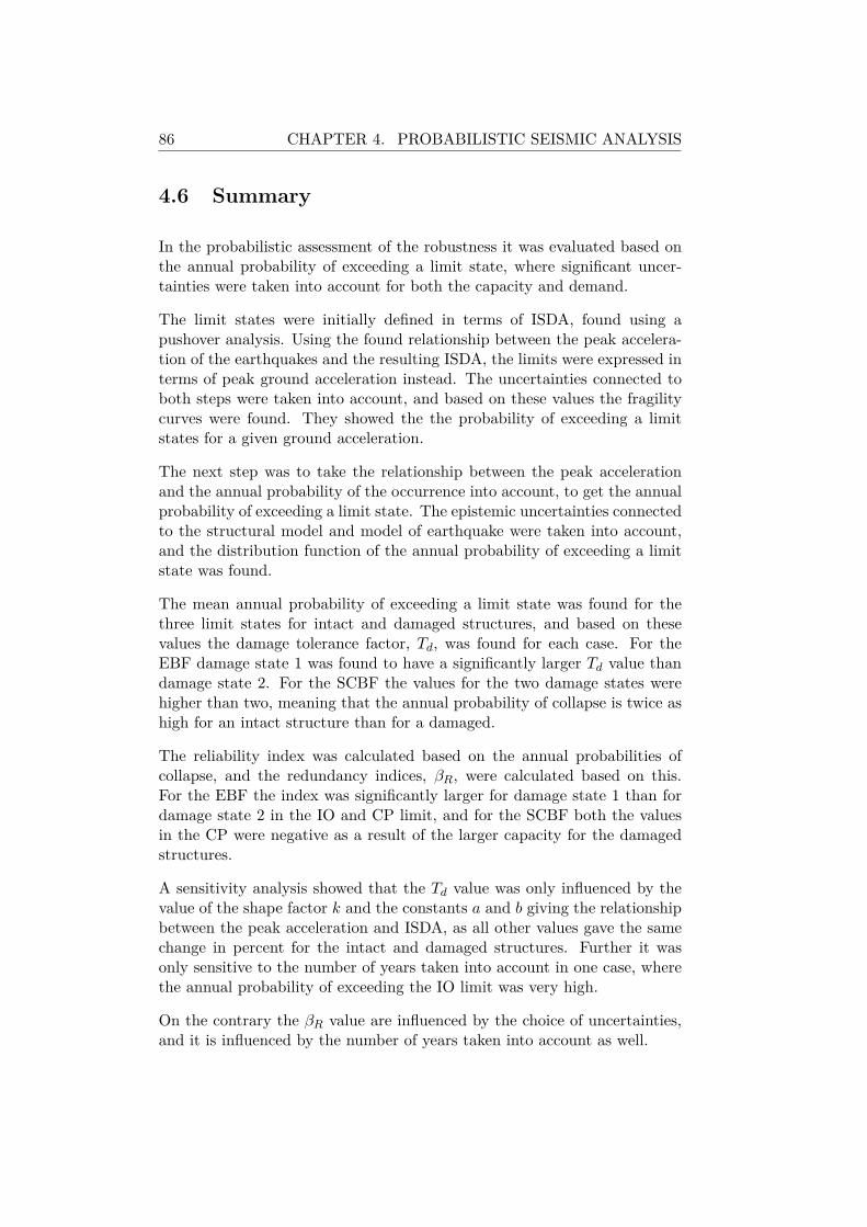
86 CHAPTER 4. PROBABILISTIC SEISMIC ANALYSIS
4.6 Summary
In the probabilistic assessment of the robustness it was evaluated based onthe annual probability of exceeding a limit state, where significant uncer-tainties were taken into account for both the capacity and demand.
The limit states were initially defined in terms of ISDA, found using apushover analysis. Using the found relationship between the peak accelera-tion of the earthquakes and the resulting ISDA, the limits were expressed interms of peak ground acceleration instead. The uncertainties connected toboth steps were taken into account, and based on these values the fragilitycurves were found. They showed the the probability of exceeding a limitstates for a given ground acceleration.
The next step was to take the relationship between the peak accelerationand the annual probability of the occurrence into account, to get the annualprobability of exceeding a limit state. The epistemic uncertainties connectedto the structural model and model of earthquake were taken into account,and the distribution function of the annual probability of exceeding a limitstate was found.
The mean annual probability of exceeding a limit state was found for thethree limit states for intact and damaged structures, and based on thesevalues the damage tolerance factor, Td, was found for each case. For theEBF damage state 1 was found to have a significantly larger Td value thandamage state 2. For the SCBF the values for the two damage states werehigher than two, meaning that the annual probability of collapse is twice ashigh for an intact structure than for a damaged.
The reliability index was calculated based on the annual probabilities ofcollapse, and the redundancy indices, βR, were calculated based on this.For the EBF the index was significantly larger for damage state 1 than fordamage state 2 in the IO and CP limit, and for the SCBF both the valuesin the CP were negative as a result of the larger capacity for the damagedstructures.
A sensitivity analysis showed that the Td value was only influenced by thevalue of the shape factor k and the constants a and b giving the relationshipbetween the peak acceleration and ISDA, as all other values gave the samechange in percent for the intact and damaged structures. Further it wasonly sensitive to the number of years taken into account in one case, wherethe annual probability of exceeding the IO limit was very high.
On the contrary the βR value are influenced by the choice of uncertainties,and it is influenced by the number of years taken into account as well.
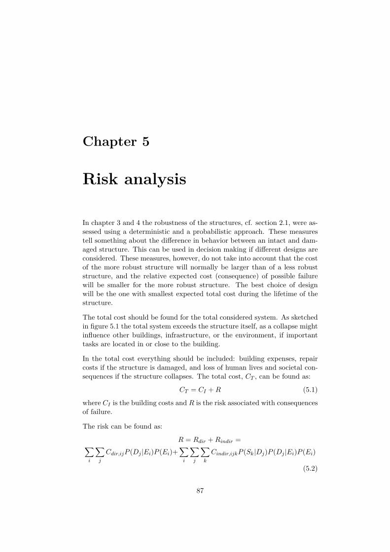
Chapter 5
Risk analysis
In chapter 3 and 4 the robustness of the structures, cf. section 2.1, were as-sessed using a deterministic and a probabilistic approach. These measurestell something about the difference in behavior between an intact and dam-aged structure. This can be used in decision making if different designs areconsidered. These measures, however, do not take into account that the costof the more robust structure will normally be larger than of a less robuststructure, and the relative expected cost (consequence) of possible failurewill be smaller for the more robust structure. The best choice of designwill be the one with smallest expected total cost during the lifetime of thestructure.
The total cost should be found for the total considered system. As sketchedin figure 5.1 the total system exceeds the structure itself, as a collapse mightinfluence other buildings, infrastructure, or the environment, if importanttasks are located in or close to the building.
In the total cost everything should be included: building expenses, repaircosts if the structure is damaged, and loss of human lives and societal con-sequences if the structure collapses. The total cost, CT , can be found as:
CT = CI +R (5.1)
where CI is the building costs and R is the risk associated with consequencesof failure.
The risk can be found as:
R = Rdir +Rindir =∑
i
∑
j
Cdir,ijP (Dj |Ei)P (Ei)+∑
i
∑
j
∑
k
Cindir,ijkP (Sk|Dj)P (Dj |Ei)P (Ei)
(5.2)
87
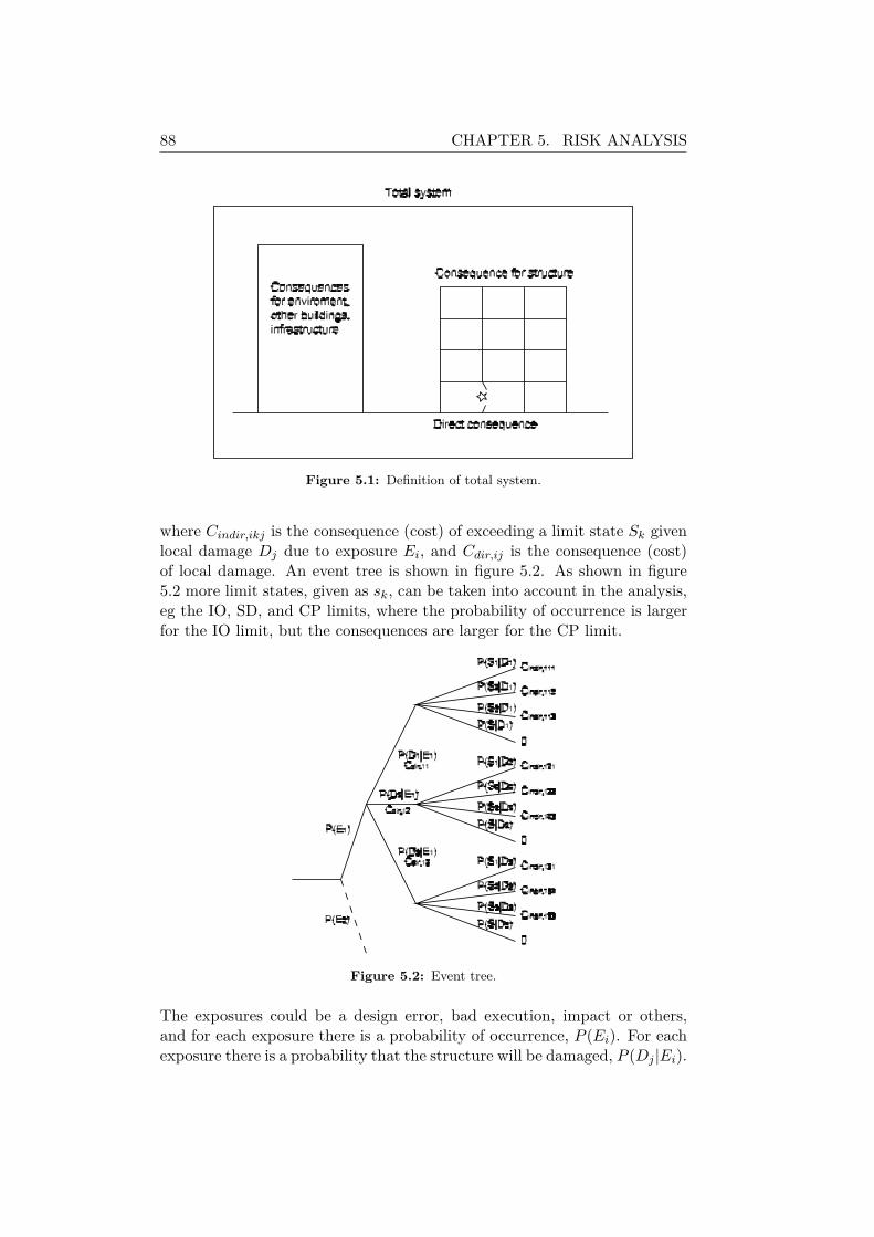
88 CHAPTER 5. RISK ANALYSIS
Figure 5.1: Definition of total system.
where Cindir,ikj is the consequence (cost) of exceeding a limit state Sk givenlocal damage Dj due to exposure Ei, and Cdir,ij is the consequence (cost)of local damage. An event tree is shown in figure 5.2. As shown in figure5.2 more limit states, given as sk, can be taken into account in the analysis,eg the IO, SD, and CP limits, where the probability of occurrence is largerfor the IO limit, but the consequences are larger for the CP limit.
Figure 5.2: Event tree.
The exposures could be a design error, bad execution, impact or others,and for each exposure there is a probability of occurrence, P (Ei). For eachexposure there is a probability that the structure will be damaged, P (Dj |Ei).
5.1. ANALYZES 89
This local damage might have a consequence Cdir,ij , but there might also be aprobability P (Sk|Dj) that the local damage leads to the exceeding of a limitstate on system level that will have the consequences Cindir,ijk. Examplesof exposures and probabilities of damage given exposures are shown in table5.1, where D1 is the intact state where there is no local damage, and D2and D3 are different damage states.
E P (E) P (D1|E) P (D2|E) P (D3|E)Large design error 0.001 0.4 0.35 0.25Small design error 0.05 0.9 0.05 0.05
Large impact 0.005 0.2 0.3 0.5Small impact 0.04 0.4 0.4 0.2
Table 5.1: Examples of exposures and probabilities of damage given exposures.
5.1 Analyzes
If different structural configurations are considered, the best choice will bethe one where the total costs, CT , is smaller. In the previous analyzes inthis project, it has been assumed that a column might be damaged. If allcolumns were designed as key elements, the design would be more expensive,but the probability that one column is damaged is smaller, and the annualprobability of collapse caused by an earthquake, will be smaller.
For a structure that is not designed for earthquake loads, an earthquakecould be regarded as an exposure in the assessment of robustness. In thiscase however the earthquake is regarded as the most crucial load designedfor, and it is taken into account with the factor P (Sk|Dj). That correspondsto the annual probability of exceeding a limit state due to earthquakes thatwas found for both intact and damaged structures in chapter 4.
To compare the two designs similar analyzes should be performed for bothstructural models. Here it is assumed that the change in design only affectsthe probability of damage Dj given the exposure Ei, given as P (Dj |Ei). Ifthe intact state is regarded as a damage state as well, the sum∑
j P (Dj |Ei)is equal to one. The assumed values of the probability of each damage stategiven an exposure are shown in table 5.2 for two different designs. Design 2is a more expensive design, where the probability of damage is smaller, andcould be a case where the columns were designed as key elements.
With these values and the annual probabilities of exceeding a limit state,found in chapter 4, the expected total cost of the two different designs canbe found, if the the probability of the exposure, the building costs, the
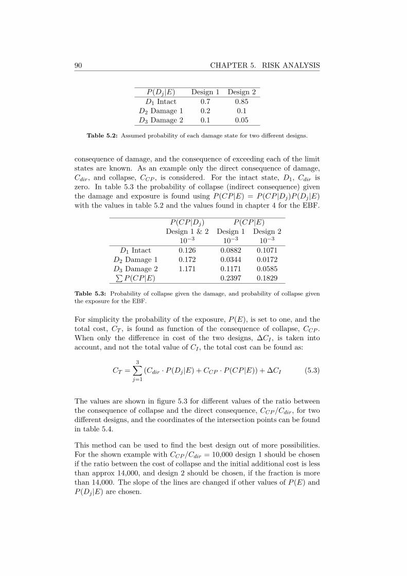
90 CHAPTER 5. RISK ANALYSIS
P (Dj |E) Design 1 Design 2D1 Intact 0.7 0.85
D2 Damage 1 0.2 0.1D3 Damage 2 0.1 0.05
Table 5.2: Assumed probability of each damage state for two different designs.
consequence of damage, and the consequence of exceeding each of the limitstates are known. As an example only the direct consequence of damage,Cdir, and collapse, CCP , is considered. For the intact state, D1, Cdir iszero. In table 5.3 the probability of collapse (indirect consequence) giventhe damage and exposure is found using P (CP |E) = P (CP |Dj)P (Dj |E)with the values in table 5.2 and the values found in chapter 4 for the EBF.
P (CP |Dj) P (CP |E)Design 1 & 2 Design 1 Design 2
10−3 10−3 10−3
D1 Intact 0.126 0.0882 0.1071D2 Damage 1 0.172 0.0344 0.0172D3 Damage 2 1.171 0.1171 0.0585∑
P (CP |E) 0.2397 0.1829
Table 5.3: Probability of collapse given the damage, and probability of collapse giventhe exposure for the EBF.
For simplicity the probability of the exposure, P (E), is set to one, and thetotal cost, CT , is found as function of the consequence of collapse, CCP .When only the difference in cost of the two designs, ∆CI , is taken intoaccount, and not the total value of CI , the total cost can be found as:
CT =3∑
j=1(Cdir · P (Dj |E) + CCP · P (CP |E)) + ∆CI (5.3)
The values are shown in figure 5.3 for different values of the ratio betweenthe consequence of collapse and the direct consequence, CCP /Cdir, for twodifferent designs, and the coordinates of the intersection points can be foundin table 5.4.
This method can be used to find the best design out of more possibilities.For the shown example with CCP /Cdir = 10,000 design 1 should be chosenif the ratio between the cost of collapse and the initial additional cost is lessthan approx 14,000, and design 2 should be chosen, if the fraction is morethan 14,000. The slope of the lines are changed if other values of P (E) andP (Dj |E) are chosen.
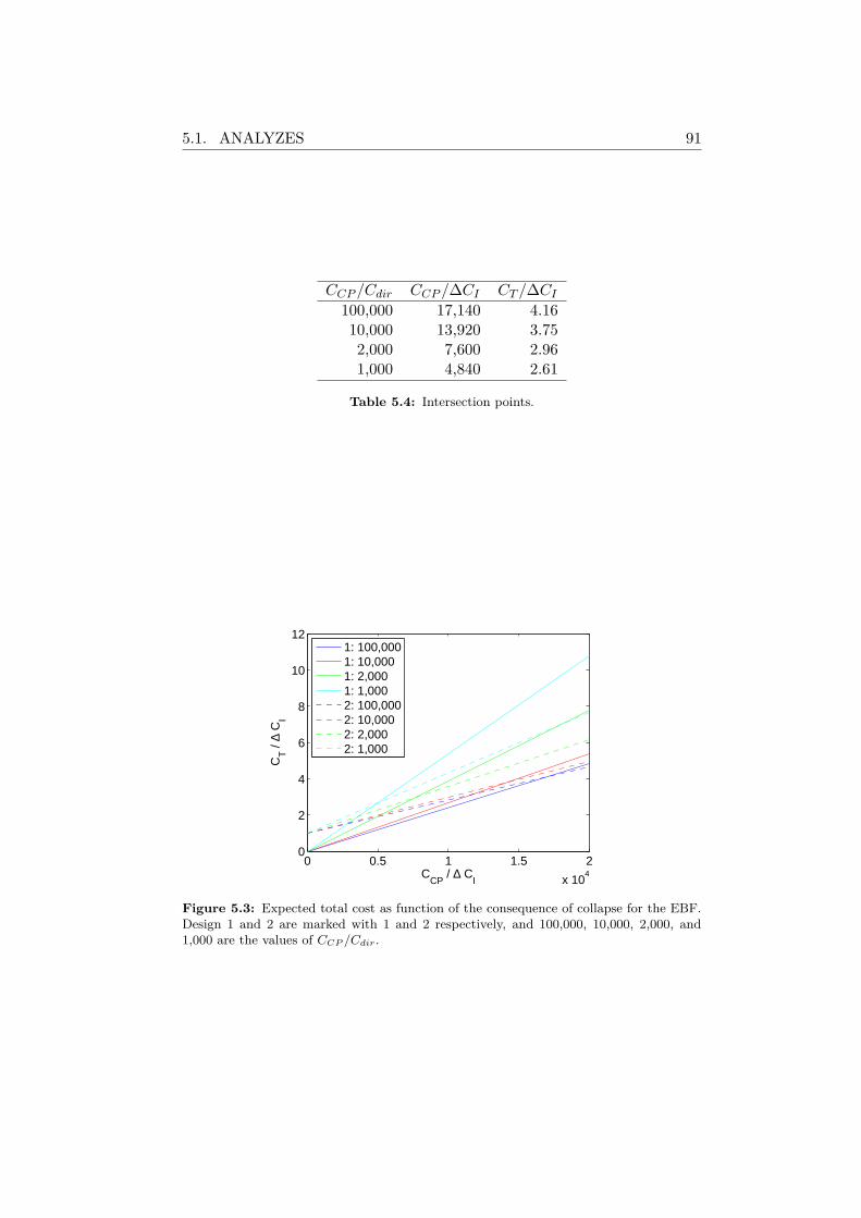
5.1. ANALYZES 91
CCP /Cdir CCP /∆CI CT /∆CI100,000 17,140 4.1610,000 13,920 3.752,000 7,600 2.961,000 4,840 2.61
Table 5.4: Intersection points.
0 0.5 1 1.5 2
x 104
0
2
4
6
8
10
12
CCP
/ ∆ CI
CT /
∆ C
I
1: 100,0001: 10,0001: 2,0001: 1,0002: 100,0002: 10,0002: 2,0002: 1,000
Figure 5.3: Expected total cost as function of the consequence of collapse for the EBF.Design 1 and 2 are marked with 1 and 2 respectively, and 100,000, 10,000, 2,000, and1,000 are the values of CCP /Cdir.
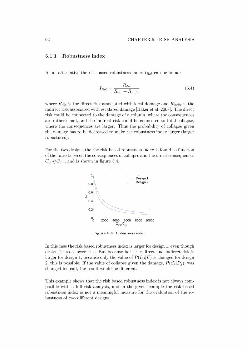
92 CHAPTER 5. RISK ANALYSIS
5.1.1 Robustness index
As an alternative the risk based robustness index IRob can be found:
IRob = RdirRdir +Rindir
(5.4)
where Rdir is the direct risk associated with local damage and Rindir is theindirect risk associated with escalated damage [Baker et al. 2008]. The directrisk could be connected to the damage of a column, where the consequencesare rather small, and the indirect risk could be connected to total collapse,where the consequences are larger. Thus the probability of collapse giventhe damage has to be decreased to make the robustness index larger (largerrobustness).
For the two designs the the risk based robustness index is found as functionof the ratio between the consequences of collapse and the direct consequencesCCP /Cdir, and is shown in figure 5.4.
0 2000 4000 6000 8000 100000
0.2
0.4
0.6
0.8
1
CCP
/Cdir
I Rob
Design 1Design 2
Figure 5.4: Robustness index.
In this case the risk based robustness index is larger for design 1, even thoughdesign 2 has a lower risk. But because both the direct and indirect risk islarger for design 1, because only the value of P (Dj |E) is changed for design2, this is possible. If the value of collapse given the damage, P (Sk|Dj), waschanged instead, the result would be different.
This example shows that the risk based robustness index is not always com-patible with a full risk analysis, and in the given example the risk basedrobustness index is not a meaningful measure for the evaluation of the ro-bustness of two different designs.
5.2. SUMMARY 93
5.2 Summary
The risk analysis is the most complete way to assess the robustness, and tochoose the best design out of more possibilities. The flaw of the method isclosely connected to the advantage, as much information is needed to makethe complete analysis. The results found in this chapter cannot be comparedwith the other methods because of limited knowledge of the values used inthe analysis.
The analysis shows how the risk analysis can be used to assess the robustness,and to rank more designs due to the expected total cost of each. In thisanalysis the damage states are linked together in a total analysis, instead ofbeing looked upon one by one.
The value of the risk based robustness index is highly dependent on the ratiobetween the consequence of collapse and the direct consequence of damage cf.figure 5.4. But as this analysis has shown, it can only be used meaningfullyif two different designs have a different value of the probability of collapsegiven the damage P (Sk|Dj). If a structure not designed for earthquakewas compared to a structure designed for earthquake there would be a bigdifference in the value of P (Sk|Dj), and the robustness index of the structuredesigned for earthquake loads would be larger.
For this analysis to make sense the damage has to be somehow caused by theearthquake or to be a hidden error eg in the design. If the damage was causedby an impact, independent of an earthquake, it would be repaired withina short time, and the probability than an earthquake would occur in thatlimited time is very small. For a hidden design error the local damage willnot have a consequence until an earthquake happens, because it would havebeen noticed and repaired in that case. This is not taken into account in thegiven example, as the probability of an earthquake should have influence onthe hidden error becoming a missing column, with the related consequences.

94 CHAPTER 5. RISK ANALYSIS
Chapter 6
Summary
In this project the robustness of two steel structures originally designed forearthquake loads in Seattle and Atlanta respectively has been assessed. Onlythe robustness in connection with horizontal loads was investigated in thisanalysis, and both deterministic, probabilistic and risk based analyzes wereused.
The seismic resistance is for both structures ensured by braces in the fa-cades, for the structure in Seattle by eccentrically braced frames (EBF)and in Atlanta by special concentrically braced frames (SCBF). For bothstructures a plane finite element model of one facade has been made, andnonlinear hinges have been assigned to reflect the post yield behavior of theelements. Nonlinear static pushover analyzes were used to find the globalnonlinear behavior of the models, and different configurations were tested toinvestigate the sensitivity of the model. The SCBF was found to have a verylimited ductile behavior, because equilibrium could not be found after thefirst failure of braces in compression. This might be caused by limitationsin the program, which is made probable by the fact that onesome of theother tested models were able to find equilibrium. The performance basedmethod in [ATC-40 1996] was used to find the performance of the structuresusing the pushover analyzes and the response spectra from the locations.
The robustness of the structures was examined by investigating the differ-ence in capacity between an intact and damaged structure, where a columnin the first floor was removed. Three limit states were investigated corre-sponding to first yield (IO), structural damage (SD) and collapse (CP). Thedrift limits were set based on the capacity curves, and the used definition ofthe SD limit was found not to be used meaningful in this kind of analysis,where damaged structures were investigated. The limit states were linked tovalues of the ground acceleration using a regression line through the found
95
96 CHAPTER 6. SUMMARY
points. The used approximation did not fit very well to the results fromthe pushover analysis, thus only two points nearest to the collapse state wasused, to give the best result.
In general the damaged structures could resist a smaller static load than theintact structure, but when the resistance against seismic loads was examinedit was found that the global ductility was very important for the capacitymeasured in terms of ground acceleration. Thus the SCBF was able to resista larger ground acceleration in the damaged cases that the intact because ofa more ductile behavior. For the EBF the intact structure performed best,but there was a big difference between the two investigated damage states.As a measure of the robustness the residual influence factor (RIF ) used inthe offshore industry was used, and it was found for the capacity measuredin terms of both the load in force and in peak ground acceleration.
To investigate the influence of the properties of the material analyzes wereperformed, where the ductility and hardening of the plastic hinges werechanged. Both a larger ductility and more hardening was found to givelarger capacities, but smaller RIF values because the ductility and hard-ening helped more for an intact structure than a damaged. However forthe damaged SCBF increased hardening seemed to hinder the global ductilebehavior, and the capacity towards seismic loads became smaller.
Probabilistic seismic analyzes were performed, where both aleatoric andepistemic uncertainties were taken into account, and the annual probabilityof exceeding a limit state was found. The seismic demand was modeled by afunction that only fitted the hazards curves provided by USGS in a limitedrange, and the fit was chosen in the point where the contribution to theprobability of exceeding a limit state was largest.
Two different probabilistic measures of the robustness was used, one basedon the probabilities of failure (Td) and one based on the reliability indices(IR). The fist gave results in the same range as the RIF values, but werein general farther away from one. This is caused by the shape of the hazardcurves. If the hazards curves had been linear the results would be equal tothe RIF values. The size of the logarithmic standard deviations used formodeling of the uncertainties did not have any influence on this measurebecause a change would work for both the intact and damaged structures.Only the relationship between a given ground acceleration and the resultingdrift had influence on the result.
The measure based on reliability indices (IR) was in another range and wastherefore harder to compare to the other. However it could be seen thatthey were not compatible as a general higher reliability gave higher redun-dancy index, where the general reliability level did not affect the Td measure.
6.1. CONCLUSION 97
Further the uncertainties and the considered range of years affected the IRmeasure.
Finally a risk based approach was used to assess the robustness, where theconsequences were taken into account. The probability of the occurrenceof damage and the exposure causing the damage were taken into account,thus the result was more accurate than the deterministic and probabilisticvalues, where it did not matter where the damage came from. In the riskbased robustness index the ratio between the direct and total risk was found.The value was highly dependent on the ratio between the consequence oflocal damage and the consequence of collapse, and was found not always tobe compatible with the result from the risk analysis.
Both the risk analysis and the different robustness indices can be used tofind the best out of more designs. The risk analysis is the most completeanalysis, but also the one than needs most information.
6.1 Conclusion
The aim of this project was to investigate whether structures designed forearthquake loads were robust too.
The common denominator in design for earthquake and robustness is theimportance of ductile behavior. For earthquake design it is necessary todissipate energy to decrease the force acting on the structure, and for ro-bustness ductility is important to make use of alternate load paths.
The analyzes have shown that the damaged structures will often have a be-havior that is different from that of the original structure, because the yield-ing mechanisms does not work the way they are designed to when membersare missing. In one damage state for the EBF the behavior was more brittle,giving a low robustness index, and in the case of the SCBF the behavior wasfound to be more ductile, giving a larger capacity. The structural configu-ration is very important for the capacity of the damaged structure, becausethe structures are less sensitive if the damage of one column only affectsone energy dissipating member, eg a shear link. This means that structuresdesigned for seismic actions will not necessarily be robust towards seismicloads, as this depends on the structural configuration.
When the robustness is investigated towards earthquake loads at least adeterministic approach, where the capacity is measured in terms of groundacceleration, should be used. The probabilistic damage tolerance factortakes the shape of the hazard curve into account, and thereby gives a valuecloser related to the annual expected damage. The reliability based index

98 CHAPTER 6. SUMMARY
takes the total reliability into account, and the structure is not ’punished’for being safer to begin with.
A risk analysis gives the most complete assessment of the robustness, andthe risk based robustness index should not be used uncritically as that maylead to wrong conclusions.
An increased capacity of the intact structure will make the structure morerobust, and only the reliability based robustness index and the risk analysistakes this into account. Both risk based approaches takes the consequencesinto account, and only the risk analysis takes the effect of a decrease of theprobability of the damage into account correct.
Increased ductility of the material was found to give a smaller deterministicrobustness, but if the reliability based index or the risk analysis was used,it would most likely be seen to increase the robustness.
In general the ductility and redundancy will provide robustness against un-foreseen vertical and horizontal loads, and human errors located in oneelement or connection. But for human errors distributed throughout thestructure redundancy will not help.

Bibliography
ASCE 7-05 [2005], American Society of Civil Engineers, New York.Minimum design loads for buildings and other structures.
ATC-40 [1996], Vol. 1, Applied Technology Council. Seismic Evaluationand Retrofit of Concrete Buildings.
Baker, J. W., Schubert, M. & Faber, M. H. [2008], ‘On the assessment ofrobustness’, Structural Safety 30(3), 253–267.
Bazeos, N. [2009], ‘Comparison of three seismic design methods for planesteel frames’, Soil Dynamics and Earthquake Engineering29(3), 553–562.
Bertero, R. D. & Bertero, V. V. [1999], ‘Redundancy inearthquake-resistant design’, Journal of Structural Engineering125(1), 81–88.
Bommer, J. J. & Pinho, R. [2006], ‘Adapting earthquake actions ineurocode 8 for performance-based seismic design’, EarthquakeEngineering and Structural Dynamics 35(1), 39–55.
Canasius, T. D. G., Sørensen, J. D. & Baker, J. W. [2007], ‘Robustness ofstructural systems’, A new focus for the Joint Committee onStructural Safety (JCSS) .
Cornell, C. A., Jalayer, F., Hamburger, R. O. & Foutch, D. A. [2002],‘Probabilistic basis for 2000 sac federal emergency managementagency steel moment frame guidelines’, Journal of StructuralEngineering 128(4), 526–533.
Dietsch, P. [2009], ‘The bad reichenhall ice-arena collapse’, COST E55 .
Ellingwood, B. R. [2001], ‘Earthquake risk assessment of buildingstructures’, Reliability Engineering and System Safety 74(3), 251–262.
99

100 BIBLIOGRAPHY
Ellingwood, B. R., Celik, O. C. & Kinali, K. [2007], ‘Fragility assessmentof building structural systems in mid-america’, EarthquakeEngineering and Structural Dynamics 36(13), 1935–1952.
Ellingwood, B. R. & Kinali, K. [2009], ‘Quantifying and communicatinguncertainty in seismic risk assessment’, Structural Safety31(2), 179–187.
Ellingwood, B. R., Smilowitz, R. & Dusenberry, D. O. [2007], BestPractices for Reducing the Potential for Progressive Collapse inBuildings, National Institute of Standards and Technology.
EN 1990:2002 [2002], European Committee for Standardization. Eurocode- Basis of structural design.
EN 1990 DK NA:2007 [2007], Erhvervs- og Byggestyrelsen. NationaltAnneks til Eurocode 0: Projekteringsgrundlag for bærendekonstruktioner.
EN 1991-1-7:2006 [2006], European Committee for Standardization.Eurocode 1 - Actions on structures - Part 1-7: General actions -Accidental actions.
EN 1998-1:2004 [2004], European Committee for Standardization.Eurocode 8 - Design of structures for earthquake resistance.
Fajfar, P. [2000], ‘A nonlinear analysis method for performance-basedseismic design’, Earthquake Spectra 16(3), 573–592.
FEMA 273 [1997], Federal Emergency Management Agency. NEHRPGuidelines for the Seismic Rehabilitation of Buildings.
Frangopol, D. M. & Curley, J. P. [1987], ‘Effects of damage andredundancy on structural reliability.’, Journal of structuralengineering New York, N.Y. 113(7), 1533–1549.
Khandelwal, K., El-Tawil, S. & Sadek, F. [2009], ‘Progressive collapseanalysis of seismically designed steel braced frames’, Journal ofConstructional Steel Research 65(3), 699–708.
Kinali, K. [2007], Seismic fragility assessment of steel frames in the centraland eastern United States, PhD thesis, Department of Civil andEnvironmental Engineering, Atlanta (GA): Georgia Institute ofTechnology.
Lind, N. C. [1995], ‘A measure of vulnerability and damage tolerance’,Reliability Engineering and System Safety 48(1), 1–6.
Munch-Andersen, J. [2009], ‘Robustness versus human errors’, COST E55 .

BIBLIOGRAPHY 101
Nair, R. S. [2006], ‘Preventing disproportionate collapse’, Journal ofPerformance of Constructed Facilities 20(4), 309–314.
Newmark, N. M. & Hall, W. J. [1982], ‘Earthquake spectra and design’,Earthquake Spectra and Design .
Nielsen, S. R. K. [2004], Vibration Theory, 3rd edn, Aalborg tekniskeUniversitetsforlag.
Poursha, M., Khoshnoudian, F. & Moghadam, A. S. [2009], ‘A consecutivemodal pushover procedure for estimating the seismic demands of tallbuildings’, Engineering Structures 31(2), 591–599.
Robobat [2008], Robot Millennium 20.1, Autodesk Inc.
Sørensen, J. D. & Christensen, H. H. [2006], ‘Danish requirements forrobustness of structures: Background and implementation’, StructuralEngineering International: Journal of the International Associationfor Bridge and Structural Engineering (IABSE) 16(2), 172–177.
Starossek, U. & Wolff, M. [2005], ‘Design of collapse resistant structures’,JCSS and IABSE Workshop on Robustness of Structures .
Straub, D. & Faber, M. H. [2005], ‘Risk based acceptance criteria for jointssubject to fatigue deterioration’, Journal of Offshore Mechanics andArctic Engineering 127(2), 150–157.
USGS [2008], U.s. geological survey national seismic hazard maps.http://earthquake.usgs.gov/research/hazmaps/products_data/2008/.
Vrouwenvelder, T. & Sørensen, J. D. [2009], ‘Robustness of structures’, EUCOST action TU0601 .
Wen, Y. K. & Song, S.-H. [2003], ‘Structural reliability/redundancy underearthquakes’, Journal of Structural Engineering 129(1), 56–67.

102 BIBLIOGRAPHY

Appendix
103


Appendix A
Time history analysis inRobot
The FEM program Robot by Robobat [Robobat 2008] has been chosen forthis project, due to it’s applicability for time history analyzes and nonlinearanalyzes. Further Robot is able to make time history analyzes, where thesupports are subjected to an acceleration time history, or alternate a dis-placement or velocity time history. However it is not clear from the manual[Robobat 2008], whether it is possible to combine these options. The ques-tion was asked to Robot support that told that the use of elasto plastic ele-ments was not recommended in a time history analysis, because of problemswith convergence and very long calculation time. Instead they suggestedthe use of nonlinear hinges. Two test setups has been made to investigate,whether Robot is able to make the required analyzes which reliable results.
A.1 Time history of linear SDOF system
The first test setup was a simple SDOF system, with a vertical weightlesscantilever beam with a point mass at the end, as shown in figure A.1. Thenatural vibration period is found to be 1.07 s.
The system is subjected to three different load cases with a horizontal forceddisplacement, forced velocity and forced acceleration time history of thesupport. The displacement time history was defined as:
d(t) = 0.2 m sin( 2π
0.8 s t)
(A.1)
105
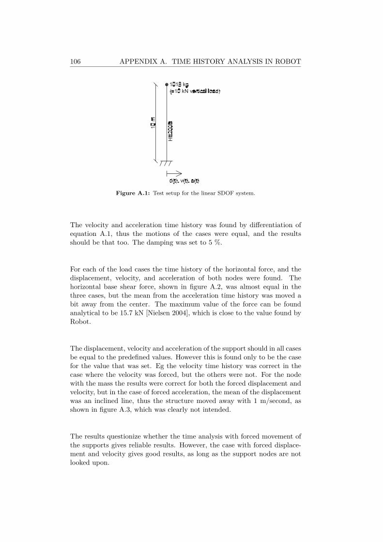
106 APPENDIX A. TIME HISTORY ANALYSIS IN ROBOT
Figure A.1: Test setup for the linear SDOF system.
The velocity and acceleration time history was found by differentiation ofequation A.1, thus the motions of the cases were equal, and the resultsshould be that too. The damping was set to 5 %.
For each of the load cases the time history of the horizontal force, and thedisplacement, velocity, and acceleration of both nodes were found. Thehorizontal base shear force, shown in figure A.2, was almost equal in thethree cases, but the mean from the acceleration time history was moved abit away from the center. The maximum value of the force can be foundanalytical to be 15.7 kN [Nielsen 2004], which is close to the value found byRobot.
The displacement, velocity and acceleration of the support should in all casesbe equal to the predefined values. However this is found only to be the casefor the value that was set. Eg the velocity time history was correct in thecase where the velocity was forced, but the others were not. For the nodewith the mass the results were correct for both the forced displacement andvelocity, but in the case of forced acceleration, the mean of the displacementwas an inclined line, thus the structure moved away with 1 m/second, asshown in figure A.3, which was clearly not intended.
The results questionize whether the time analysis with forced movement ofthe supports gives reliable results. However, the case with forced displace-ment and velocity gives good results, as long as the support nodes are notlooked upon.
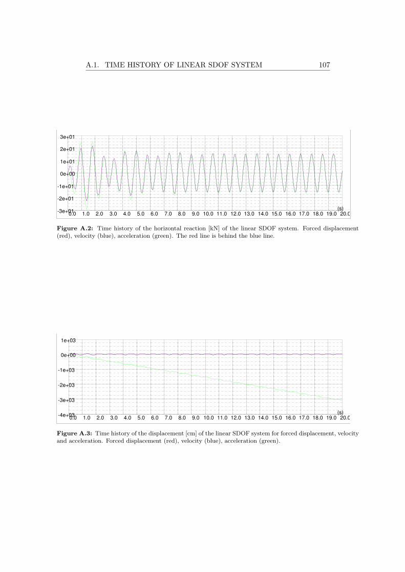
A.1. TIME HISTORY OF LINEAR SDOF SYSTEM 107
0.0 1.0 2.0 3.0 4.0 5.0 6.0 7.0 8.0 9.0 10.0 11.0 12.0 13.0 14.0 15.0 16.0 17.0 18.0 19.0 20.0-3e+01
-2e+01
-1e+01
0e+00
1e+01
2e+01
3e+01
(s)
Figure A.2: Time history of the horizontal reaction [kN] of the linear SDOF system. Forced displacement(red), velocity (blue), acceleration (green). The red line is behind the blue line.
0.0 1.0 2.0 3.0 4.0 5.0 6.0 7.0 8.0 9.0 10.0 11.0 12.0 13.0 14.0 15.0 16.0 17.0 18.0 19.0 20.0-4e+03
-3e+03
-2e+03
-1e+03
0e+00
1e+03
(s)
Figure A.3: Time history of the displacement [cm] of the linear SDOF system for forced displacement, velocityand acceleration. Forced displacement (red), velocity (blue), acceleration (green).
108 APPENDIX A. TIME HISTORY ANALYSIS IN ROBOT
A.2 Time history of nonlinear SDOF system
To test whether the nonlinear solver gives reliable results for a time historyanalysis with forced movements of the support, the linear problem is solvedusing the implemented nonlinear solvers. It is possible to choose betweenNewmark (acceleration) and Hilbert-Huges-Taylor. Both solvers were usedfor both forced displacement, velocity and acceleration, but in all cases theyeither gave the result zero, did not converge, or in case of forced acceleration,had the same problem as the linear solver.
A.3 Conclusion on tests
Based on the investigations it can be concluded that the nonlinear timehistory analyzes with moving supports in Robot are not sufficient reliableto be used for the analyzes in this project. Alternatively an other programcould be used, but due to limited time and resources it is chosen to use asimpler analysis type, the static pushover analysis.
Appendix B
Nonlinear static performancebased analysis
This appendix describes the nonlinear performance based analysis procedureused in [ATC-40 1996]. The method is used to find the performance of astructure for a specific elastic response spectrum, when a static pushoveranalysis has been performed, and the capacity curve is found cf. section1.1.1. There exist other methods for this task, eg the method proposed by[Fajfar 2000] and the method used in [EN 1998-1:2004 2004]. The methodfrom [ATC-40 1996] is chosen because it is build into the finite elementsoftware Robot, and because the method provides a clear sight into how thehysteretic energy dissipation is taken into account, even though only a staticanalysis is performed.
B.1 Capacity curve
To get the capacity curve, is it necessary to complete a static pushoveranalysis. First a modal analysis is performed to find the mode shapes of thestructure. Based on the mass distribution of the structure and the modeshape with largest mass participation, a set of lateral forces is applied tothe structure. The force is increased in small steps until collapse is reached.Then a capacity curve with the base shear force as function of the horizontalroof displacement can be plotted. The procedure is shown in figure B.1.
109
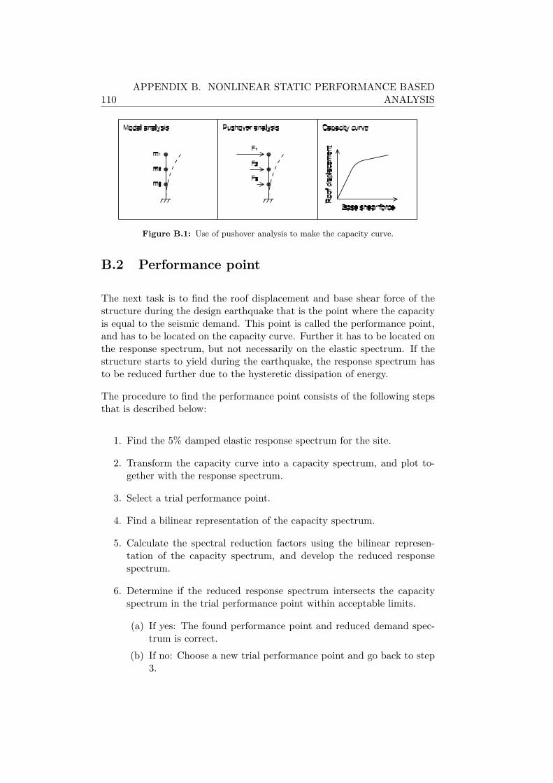
110APPENDIX B. NONLINEAR STATIC PERFORMANCE BASED
ANALYSIS
Figure B.1: Use of pushover analysis to make the capacity curve.
B.2 Performance point
The next task is to find the roof displacement and base shear force of thestructure during the design earthquake that is the point where the capacityis equal to the seismic demand. This point is called the performance point,and has to be located on the capacity curve. Further it has to be located onthe response spectrum, but not necessarily on the elastic spectrum. If thestructure starts to yield during the earthquake, the response spectrum hasto be reduced further due to the hysteretic dissipation of energy.
The procedure to find the performance point consists of the following stepsthat is described below:
1. Find the 5% damped elastic response spectrum for the site.
2. Transform the capacity curve into a capacity spectrum, and plot to-gether with the response spectrum.
3. Select a trial performance point.
4. Find a bilinear representation of the capacity spectrum.
5. Calculate the spectral reduction factors using the bilinear represen-tation of the capacity spectrum, and develop the reduced responsespectrum.
6. Determine if the reduced response spectrum intersects the capacityspectrum in the trial performance point within acceptable limits.
(a) If yes: The found performance point and reduced demand spec-trum is correct.
(b) If no: Choose a new trial performance point and go back to step3.
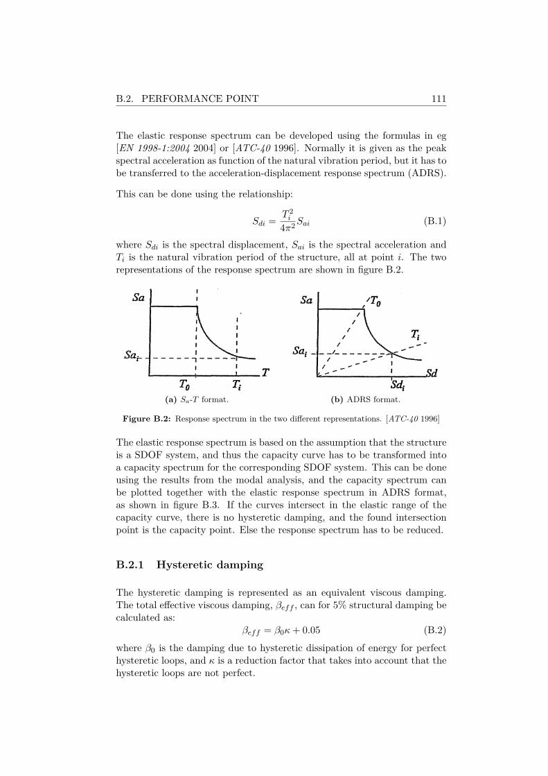
B.2. PERFORMANCE POINT 111
The elastic response spectrum can be developed using the formulas in eg[EN 1998-1:2004 2004] or [ATC-40 1996]. Normally it is given as the peakspectral acceleration as function of the natural vibration period, but it has tobe transferred to the acceleration-displacement response spectrum (ADRS).
This can be done using the relationship:
Sdi = T 2i
4π2Sai (B.1)
where Sdi is the spectral displacement, Sai is the spectral acceleration andTi is the natural vibration period of the structure, all at point i. The tworepresentations of the response spectrum are shown in figure B.2.
(a) Sa-T format. (b) ADRS format.
Figure B.2: Response spectrum in the two different representations. [ATC-40 1996]
The elastic response spectrum is based on the assumption that the structureis a SDOF system, and thus the capacity curve has to be transformed intoa capacity spectrum for the corresponding SDOF system. This can be doneusing the results from the modal analysis, and the capacity spectrum canbe plotted together with the elastic response spectrum in ADRS format,as shown in figure B.3. If the curves intersect in the elastic range of thecapacity curve, there is no hysteretic damping, and the found intersectionpoint is the capacity point. Else the response spectrum has to be reduced.
B.2.1 Hysteretic damping
The hysteretic damping is represented as an equivalent viscous damping.The total effective viscous damping, βeff , can for 5% structural damping becalculated as:
βeff = β0κ+ 0.05 (B.2)
where β0 is the damping due to hysteretic dissipation of energy for perfecthysteretic loops, and κ is a reduction factor that takes into account that thehysteretic loops are not perfect.
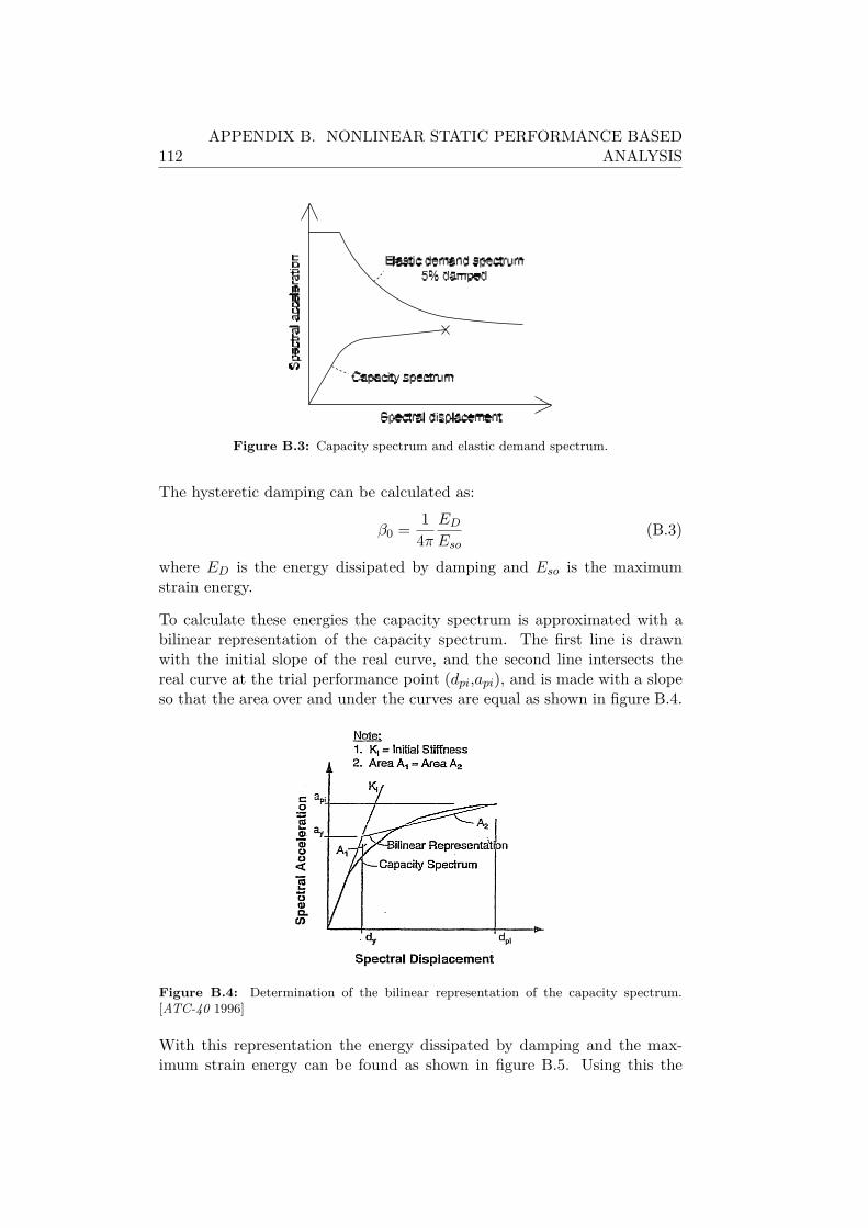
112APPENDIX B. NONLINEAR STATIC PERFORMANCE BASED
ANALYSIS
Figure B.3: Capacity spectrum and elastic demand spectrum.
The hysteretic damping can be calculated as:
β0 = 14π
EDEso
(B.3)
where ED is the energy dissipated by damping and Eso is the maximumstrain energy.
To calculate these energies the capacity spectrum is approximated with abilinear representation of the capacity spectrum. The first line is drawnwith the initial slope of the real curve, and the second line intersects thereal curve at the trial performance point (dpi,api), and is made with a slopeso that the area over and under the curves are equal as shown in figure B.4.
Figure B.4: Determination of the bilinear representation of the capacity spectrum.[ATC-40 1996]
With this representation the energy dissipated by damping and the max-imum strain energy can be found as shown in figure B.5. Using this the
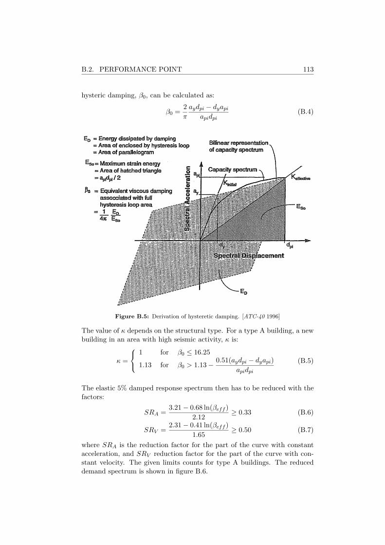
B.2. PERFORMANCE POINT 113
hysteric damping, β0, can be calculated as:
β0 = 2π
aydpi − dyapiapidpi
(B.4)
Figure B.5: Derivation of hysteretic damping. [ATC-40 1996]
The value of κ depends on the structural type. For a type A building, a newbuilding in an area with high seismic activity, κ is:
κ =
1 for β0 ≤ 16.25
1.13 for β0 > 1.13− 0.51(aydpi − dyapi)apidpi
(B.5)
The elastic 5% damped response spectrum then has to be reduced with thefactors:
SRA = 3.21− 0.68 ln(βeff )2.12 ≥ 0.33 (B.6)
SRV = 2.31− 0.41 ln(βeff )1.65 ≥ 0.50 (B.7)
where SRA is the reduction factor for the part of the curve with constantacceleration, and SRV reduction factor for the part of the curve with con-stant velocity. The given limits counts for type A buildings. The reduceddemand spectrum is shown in figure B.6.
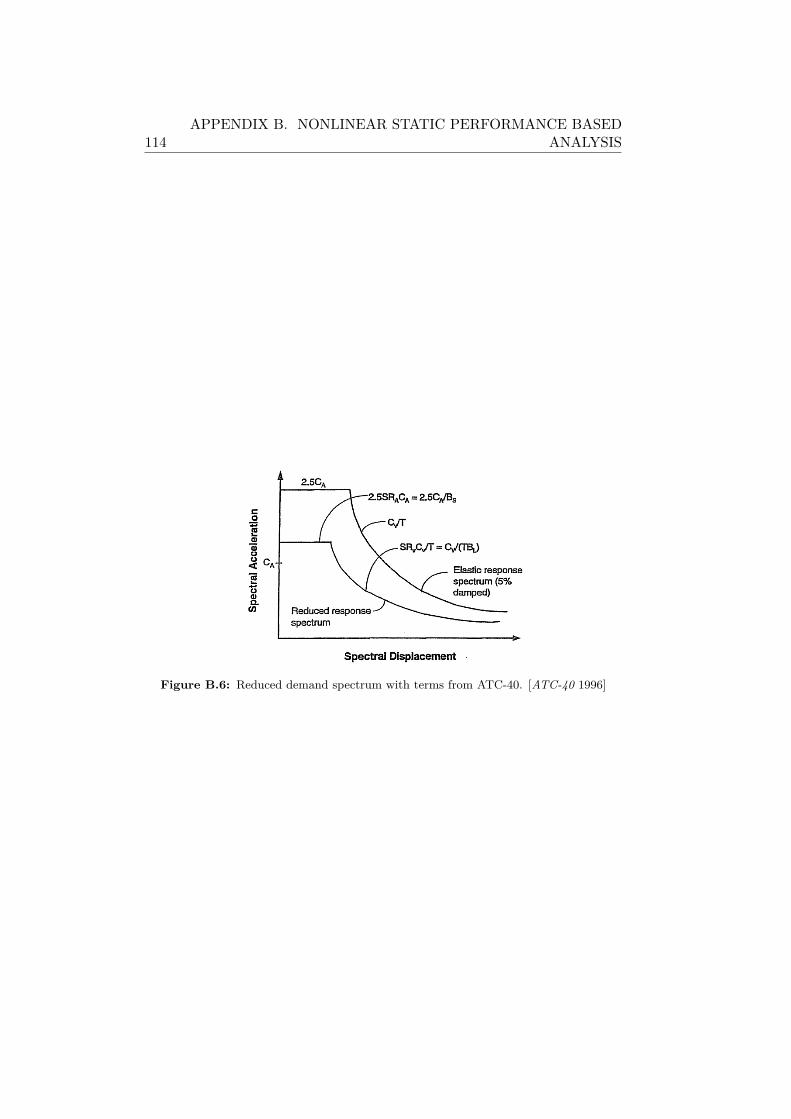
114APPENDIX B. NONLINEAR STATIC PERFORMANCE BASED
ANALYSIS
Figure B.6: Reduced demand spectrum with terms from ATC-40. [ATC-40 1996]

Appendix C
Programs
The enclosed CD contains MATLAB programs used for the calculations inthis project. The major files are listed below and in addition a number ofinput files can be found on the cd.
main_deterministic.m Main file for deterministic analyzes
main_probabilistic.m Main file for probabilistic analyzes
pushover.m Function that calculates step nr. for the SD limit and perfor-mance points
isdaldef.m Function that calculates ISDA
powerreg.m Function that performs regression for ISDA-Sa relationship
hazard.m Function with data for seismic hazard curves
fragility.m Function that calculates the fragility curves and the annualprobability of exceeding a limit state
hazardcurve.m Calculates fit to data from USGS
riskanalysis.m Calculations for the risk analysis
Irob.m Calculations for the risk based robustness index
sensitivitytears.m Calculates probabilistic indices for a number of years
115