
Probabilistic Analysis of a Monod-type equation by use of … · 2008-08-12 · and the...
34
Probabilistic Analysis of a Monod-type equation by use of a single chamber Microbial Fuel Cell Eric A. Zielke December 9, 2005
Transcript of Probabilistic Analysis of a Monod-type equation by use of … · 2008-08-12 · and the...
Probabilistic Analysis of a Monod-type equation by useof a single chamber Microbial Fuel Cell
Eric A. Zielke
December 9, 2005
i
Abstract
Renewable energy forms have become an increasing need for our society. Microbial fuelcells (MFCs) represent a new form of renewable energy by converting organic matter intoelectricity by using bacteria already present in wastewater while simultaneously treating thewastewater. Most of the current research on MFCs is concerned with increasing the powerof the system with respect to the peripheral anode surface area; little research has beendone on determining the effects of uncertainty associated with the power density. The powerdensity produced in a MFC can be modeled as a function of substrate concentration usingan empirical Monod-type equation. This particular study used a Monte Carlo simulationto demonstrate that the uncertainty intrinsic to the parameters of maximum power densityand the half-saturation constant associated with the Monod-type equation by use of a singlechamber Microbial Fuel Cell affect the power density produced in the Microbial Fuel Cell.The Monte Carlo simulation was used to justify the uncertainty associated with power densityto be a continuous uniform distribution. The simulation determined that the maximumpower density parameter from the Monod-type equation has a greater effect on power density,P , then the half-saturation constant parameter. Given the same probability range, the powerdensity exhibited a range of 93.29 to 227.1 mW/m2 when the maximum power density wasused in the Monte Carlo simulation in comparison to a range of 226.7 to 254.3 mW/m2 of thepower density when the half-saturation constant was used in the Monte Carlo simulation.A derived distribution was determined for the power density assuming a normal populationdistribution. The Chebyshev inequality determined a probability of P [P ≤ (29720)] ≥ 0.75corresponding to 2 sigma bounds. A Taylor series approximation of the mean and variancecorresponded to values of 259.1 and 14720.
Probabilistic Analysis Zielke ii
Contents
1 Introduction 1
2 Problem Formulation 2
3 Literature Review 2
3.1 The Monod Model . . . . . . . . . . . . . . . . . . . . . . . . . . . . . . . . 3
3.2 Parameter Uncertainty . . . . . . . . . . . . . . . . . . . . . . . . . . . . . . 3
4 Model Formulation and Development 4
4.1 Model Assumptions and Limitations . . . . . . . . . . . . . . . . . . . . . . 6
5 Model Application 6
5.1 Characterizing Uncertainty in the Model Parameters . . . . . . . . . . . . . 6
5.2 Random Number Generation . . . . . . . . . . . . . . . . . . . . . . . . . . . 8
5.3 Validation of the Random Variable . . . . . . . . . . . . . . . . . . . . . . . 11
5.3.1 Chi-Squared Test . . . . . . . . . . . . . . . . . . . . . . . . . . . . . 11
5.3.2 Kolmogorov-Smirnov Test . . . . . . . . . . . . . . . . . . . . . . . . 13
5.4 Monte Carlo Application . . . . . . . . . . . . . . . . . . . . . . . . . . . . . 14
6 Model Results 14
6.1 Monte Carlo results . . . . . . . . . . . . . . . . . . . . . . . . . . . . . . . . 16
6.2 Validation of the Monod Model’s State Variable . . . . . . . . . . . . . . . . 16
6.3 Calculating Probabilities and Random Variables from the Cumulative Distri-butions . . . . . . . . . . . . . . . . . . . . . . . . . . . . . . . . . . . . . . . 19
6.4 Derived Probability Distribution . . . . . . . . . . . . . . . . . . . . . . . . . 22
Probabilistic Analysis Zielke iii
6.5 Chebyshev inequality . . . . . . . . . . . . . . . . . . . . . . . . . . . . . . . 22
6.6 Taylor Series Approximation . . . . . . . . . . . . . . . . . . . . . . . . . . . 23
7 Conclusions 24
8 Further Research 25
9 References 26
10 Appendix 28
Probabilistic Analysis Zielke iv
List of Figures
1 Graphical display of 100 randomly generated numbers. (a) Histogram of max-imum power density data; (b) cumulative frequency distribution of maximumpower density data. . . . . . . . . . . . . . . . . . . . . . . . . . . . . . . . . 9
2 Graphical display of 100 randomly generated numbers. (a) Histogram ofhalf-saturation constant data; (b) cumulative frequency distribution of half-saturation constant data. . . . . . . . . . . . . . . . . . . . . . . . . . . . . . 10
3 Empirical cumulative frequency vs. theoretical distribution function (a) Rep-resentative of maximum power density, Pmax (mW/m2); (b) representative ofhalf-saturation constant, Ks (mg/L). . . . . . . . . . . . . . . . . . . . . . . 15
4 Histogram of evaluating the random variable associated with state variableP (mW/m2) (a) by changing Pmax (mW/m2) while holding the parameterof Ks constant at the average value of randomly generated numbers; (b) bychanging Ks (mg/L) while holding the parameter of Pmax (mW/m2) constantat the average value of randomly generated numbers. . . . . . . . . . . . . . 17
5 Empirical cumulative frequency vs. theoretical distribution function (a) Rep-resentative of power density, P , by changing the maximum power density,Pmax (mW/m2); (b) representative of power density, P , by changing the half-saturation constant, Ks (mg/L). . . . . . . . . . . . . . . . . . . . . . . . . . 21
Probabilistic Analysis Zielke v
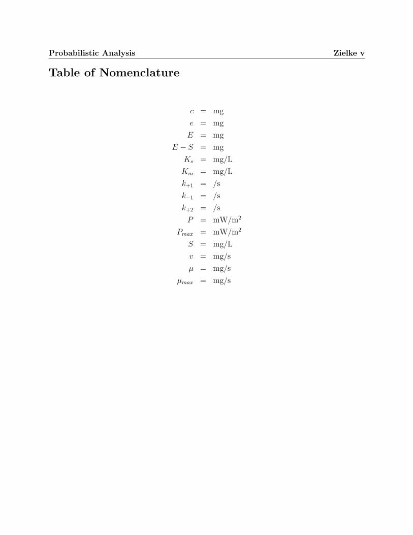
Table of Nomenclature
c = mg
e = mg
E = mg
E − S = mg
Ks = mg/L
Km = mg/L
k+1 = /s
k−1 = /s
k+2 = /s
P = mW/m2
Pmax = mW/m2
S = mg/L
v = mg/s
µ = mg/s
µmax = mg/s
Probabilistic Analysis Zielke 1
1 Introduction
Renewable energy has become an increasing need to our society. Microbial fuel cell (MFC)
technology represents a new form of renewable energy by generating electricity from what
would otherwise be considered waste. This technology can use bacteria already present in
wastewater as a catalyst to electricity generation while simultaneously treating wastewater
(Lui et al., 2004, Min and Logan, 2004). Although MFCs generate a lower amount of
energy than hydrogen fuel cells, a combination of both electricity production and wastewater
treatment may help reduce the cost of treating primary effluent wastewater.
A typical MFC consists of two chambers separated by a Proton Exchange Membrane
(PEM) such as Nafion (Oh et al. 2004). The disadvantage of the two chamber system is
that the cathode chamber needs to be filled with a chemical liquid and aerated to provide
oxygen to the cathode (Lui et al., 2004). In hydrogen fuel cells, the cathode is bonded to
the PEM which allows oxygen from the air to directly react at the cathode. This same
principle is used on single chamber MFCs where the anode chamber is separated from the
air-cathode chamber by a gas diffusion layer (GDL) allowing oxygen from the air to transfer
to the cathode (Lui et al., 2004). This eliminates the need for energy intensive air sparging
of a chemical liquid such as ferrocyanide (Lui et al., 2004). Power generation of a single
chamber MFC has been shown in the absence of a PEM decreasing the overall cost (Lui et
al., 2004).
The power density produced in a single chamber MFC can be modeled as a function
of substrate concentration using an empirical Monod-type equation (Lui et al. 2005). This
algebraic equation exhibits power density as a state variable, substrate concentration as
the independent variable, and maximum power density and the half-saturation constant as
parameters (Lui et al. 2005). This particular equation uses empirical data of the power
density and substrate concentration to solve for the parameters. The parameters are then
used to develop a function of power density, the state variable, versus substrate concentration,
Probabilistic Analysis Zielke 2
the independent variable following that of enzyme reaction kinetics (Aiba et al., 1965).
There exists uncertainty between the parameters within the Monod-type equation due
to correlations between them (Liu, 2001). These uncertainties will effect the value of the
power density. The probabilistic analysis of the this model will include a Monte Carlo
simulation to develop histograms displaying frequency diagrams and cumulative frequency
diagrams pertaining to power density. A better understanding of how these uncertainties
effect the power density in this model will lead the way to a better understanding of how to
improve the power density and, ultimately, the design of the MFC.
2 Problem Formulation
The objective of this study is to analyze data of the model variables from experimentation of
a single chamber MFC to determine the range of values these parameters exhibit. Random
numbers will then be generated by a random number generator intrinsic to the Microsoft
Excel computer program to use as the population model. The population model will be
validated by the chi-squared test, and K-S test. The population model of the random num-
bers will be computed according to the Monod-type equation for a Monte Carlo simulation.
This simulation will be used to develop histograms displaying the frequency diagrams and
cumulative frequency diagrams to determine how the effects of uncertainty change the value
of the power density.
3 Literature Review
The purpose of this literature review is to organize relevent information to refer back to in an
optimal fashion when applying principles of probablistic analysis to the Monod-type equation
Probabilistic Analysis Zielke 3
used on a MFC. This section contains an overview of the Monod model and uncertainties
within the parameters of the model.
3.1 The Monod Model
The Monod model can describe several important characteristics of microbial growth in
a simple periodic culture of microorganisms (Dette et al., 2003). This model was first
proposed by Nobel Laureate J. Monod more then 50 years ago and is one of the basic models
for quantitative microbiology (Monod, 1949; Dette et al., 2003). This model is typically
defined by a differential equation (Dette et al., 2003). Many limitations of this model as
well as restrictions of its applications are well known (Pirt, 1975; Baranyi and Roberts,
1995; Ferenci, 1999; Dette et al., 2003). With these limitations, many modifications of the
model have also been proposed within specific cases (Ellis et al., 1996; Fu and Mathews,
1999; Schirmer et al., 1999; Vanrolleghem et al., 1999; Dette et al., 2003). The Monod-type
equation used in this analysis is in an algebraic form under the assumption of a steady state
condition.
3.2 Parameter Uncertainty
Within one specific study on a single chamber MFC, a change in the experimental condi-
tions varied the half-saturation constant from 9-141 mg/L and the maximum power density
from 86-661mW/m2 (Lui et al, 2005). One study suggested the Monod model parameters
are correlated to each other linearly and are not to be considered statistically independent
(Liu et al., 2001). However, this particular study will make the assumption of statistical
independence between the models parameters. Since no distribution has ever been proposed
on a specific case such as this, this study will assume the parameters of maximum power
Probabilistic Analysis Zielke 4
density and the half-saturation constant within this model are random, uniformly distributed
variables.
4 Model Formulation and Development
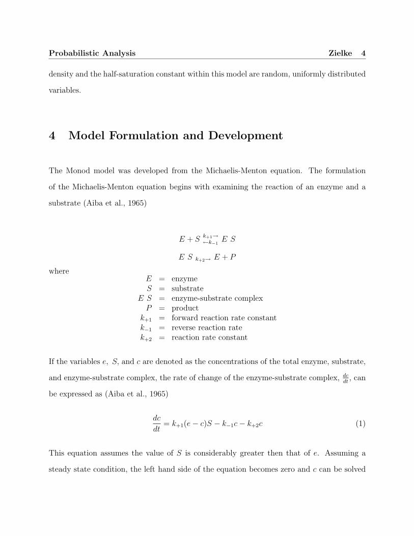
The Monod model was developed from the Michaelis-Menton equation. The formulation
of the Michaelis-Menton equation begins with examining the reaction of an enzyme and a
substrate (Aiba et al., 1965)
E + Sk+1→←k−1
E S
E S k+2→ E + P
whereE = enzymeS = substrate
E S = enzyme-substrate complexP = product
k+1 = forward reaction rate constantk−1 = reverse reaction ratek+2 = reaction rate constant
If the variables e, S, and c are denoted as the concentrations of the total enzyme, substrate,
and enzyme-substrate complex, the rate of change of the enzyme-substrate complex, dcdt
, can
be expressed as (Aiba et al., 1965)
dc
dt= k+1(e− c)S − k−1c− k+2c (1)
This equation assumes the value of S is considerably greater then that of e. Assuming a
steady state condition, the left hand side of the equation becomes zero and c can be solved
Probabilistic Analysis Zielke 5
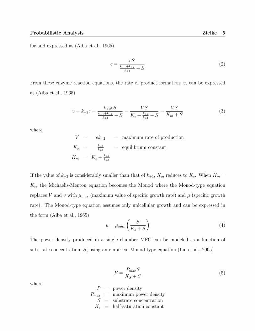
for and expressed as (Aiba et al., 1965)
c =eS
k−1+k+2
k+1+ S
(2)
From these enzyme reaction equations, the rate of product formation, v, can be expressed
as (Aiba et al., 1965)
v = k+2c =k+2eS
k−1+k+2
k+1+ S
=V S
Ks + k+2
k+1+ S
=V S
Km + S(3)
where
V = ek+2 = maximum rate of production
Ks = k−1
k+1= equilibrium constant
Km = Ks + k+2
k+1
If the value of k+2 is considerably smaller than that of k+1, Km reduces to Ks. When Km =
Ks, the Michaelis-Menton equation becomes the Monod where the Monod-type equation
replaces V and v with µmax (maximum value of specific growth rate) and µ (specific growth
rate). The Monod-type equation assumes only unicellular growth and can be expressed in
the form (Aiba et al., 1965)
µ = µmax
(S
Ks + S
)(4)
The power density produced in a single chamber MFC can be modeled as a function of
substrate concentration, S, using an empirical Monod-type equation (Lui et al., 2005)
P =PmaxS
KS + S(5)
whereP = power density
Pmax = maximum power densityS = substrate concentration
Ks = half-saturation constant
Probabilistic Analysis Zielke 6
4.1 Model Assumptions and Limitations
The progression from equation (1) to (2) assumes that substrate concentration will greatly
exceed that of the total enzyme concentration. Equation (2) assumes a steady state con-
dition. The later assumption suggests the model’s state variable varies only with substrate
concentration and not time. The progression of equation (3) to (4) assumes the forward
reaction rate constant to be much greater then that of the reverse reaction rate, i.e. Km
is replaced with Ks (Aiba et al., 1965). The assumption of equation (4) is based on ob-
servations of unicellular growth limited by a single substrate type. Equation (5) replaces µ
and µmax with P and Pmax suggesting power density to act according to the specific growth
rate of microorganisms. The model used in this particular study will assume statistical in-
dependence of the parameters, Pmax and Ks even though case studies of similar monod-type
equations have stated these parameters are not statistically independent (Liu et al., 2001).
5 Model Application
This section details the primer process of the Monte Carlo method. This includes the char-
acterization of uncertainty in the model parameters, random number generation and the
validation of the random variable to each parameter Ks and Pmax.
5.1 Characterizing Uncertainty in the Model Parameters
The probability density function and the mathematical expectation value and variance of
the random variable are represented when characterizing the uncertainty of a probability
distribution. For a continuous random variable, X, along the interval (a, b) the probability
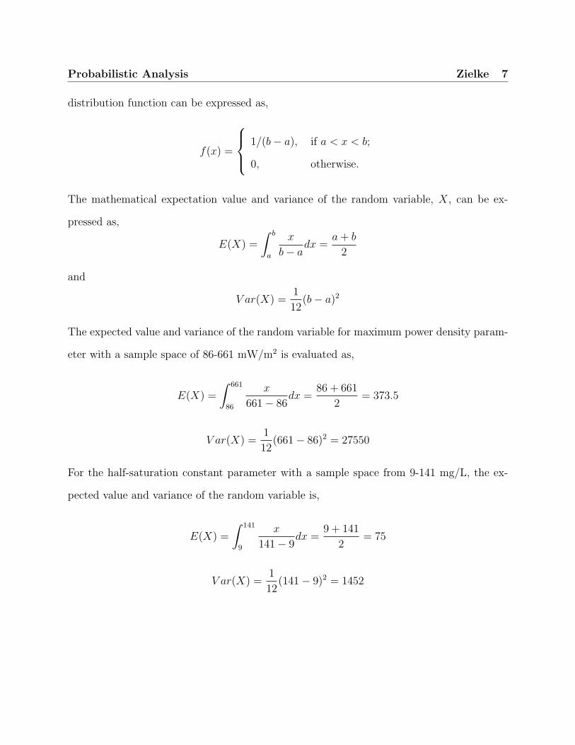
Probabilistic Analysis Zielke 7
distribution function can be expressed as,
f(x) =
1/(b− a), if a < x < b;
0, otherwise.
The mathematical expectation value and variance of the random variable, X, can be ex-
pressed as,
E(X) =
∫ b
a
x
b− adx =
a + b
2
and
V ar(X) =1
12(b− a)2
The expected value and variance of the random variable for maximum power density param-
eter with a sample space of 86-661 mW/m2 is evaluated as,
E(X) =
∫ 661
86
x
661− 86dx =
86 + 661
2= 373.5
V ar(X) =1
12(661− 86)2 = 27550
For the half-saturation constant parameter with a sample space from 9-141 mg/L, the ex-
pected value and variance of the random variable is,
E(X) =
∫ 141
9
x
141− 9dx =
9 + 141
2= 75
V ar(X) =1
12(141− 9)2 = 1452
Probabilistic Analysis Zielke 8
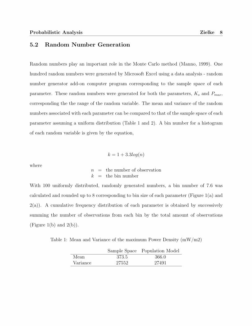
5.2 Random Number Generation
Random numbers play an important role in the Monte Carlo method (Manno, 1999). One
hundred random numbers were generated by Microsoft Excel using a data analysis - random
number generator add-on computer program corresponding to the sample space of each
parameter. These random numbers were generated for both the parameters, Ks and Pmax,
corresponding the the range of the random variable. The mean and variance of the random
numbers associated with each parameter can be compared to that of the sample space of each
parameter assuming a uniform distribution (Table 1 and 2). A bin number for a histogram
of each random variable is given by the equation,
k = 1 + 3.3log(n)
wheren = the number of observationk = the bin number
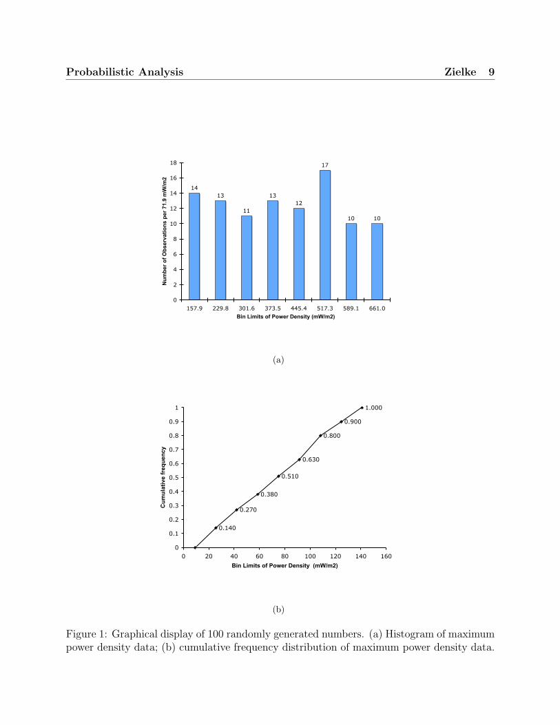
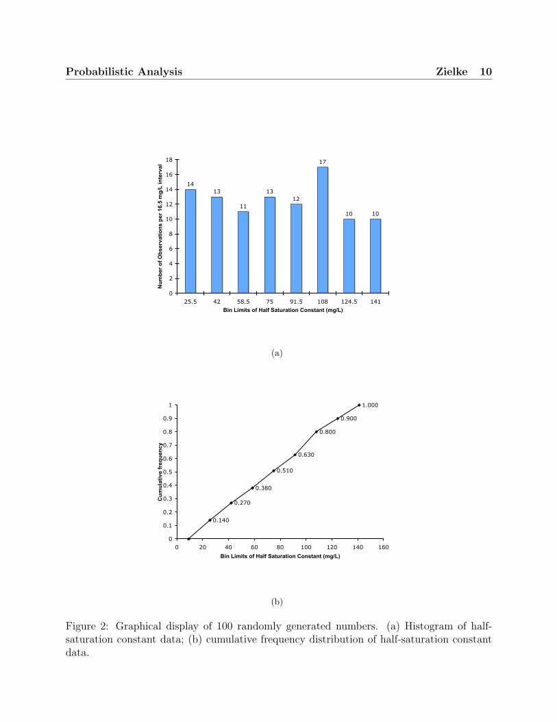
With 100 uniformly distributed, randomly generated numbers, a bin number of 7.6 was
calculated and rounded up to 8 corresponding to bin size of each parameter (Figure 1(a) and
2(a)). A cumulative frequency distribution of each parameter is obtained by successively
summing the number of observations from each bin by the total amount of observations
(Figure 1(b) and 2(b)).
Table 1: Mean and Variance of the maximum Power Density (mW/m2)
Sample Space Population ModelMean 373.5 366.0Variance 27552 27491
Probabilistic Analysis Zielke 9
1010
17
1213
11
1413
0
2
4
6
8
10
12
14
16
18
157.9 229.8 301.6 373.5 445.4 517.3 589.1 661.0Bin Limits of Power Density (mW/m2)
Num
ber o
f Obs
erva
tions
per
71.
9 m
W/m
2
(a)
0.140
0.270
0.380
0.510
0.630
0.800
0.900
1.000
0
0.1
0.2
0.3
0.4
0.5
0.6
0.7
0.8
0.9
1
0 20 40 60 80 100 120 140 160
Bin Limits of Power Density (mW/m2)
Cum
ulat
ive
freq
uenc
y
(b)
Figure 1: Graphical display of 100 randomly generated numbers. (a) Histogram of maximumpower density data; (b) cumulative frequency distribution of maximum power density data.
Probabilistic Analysis Zielke 10
1413
11
1312
17
10 10
0
2
4
6
8
10
12
14
16
18
25.5 42 58.5 75 91.5 108 124.5 141Bin Limits of Half Saturation Constant (mg/L)
Num
ber o
f Obs
erva
tions
per
16.
5 m
g/L
inte
rval
(a)
0.140
0.270
0.380
0.510
0.630
0.800
0.900
1.000
0
0.1
0.2
0.3
0.4
0.5
0.6
0.7
0.8
0.9
1
0 20 40 60 80 100 120 140 160
Bin Limits of Half Saturation Constant (mg/L)
Cum
ulat
ive
freq
uenc
y
(b)
Figure 2: Graphical display of 100 randomly generated numbers. (a) Histogram of half-saturation constant data; (b) cumulative frequency distribution of half-saturation constantdata.
Probabilistic Analysis Zielke 11
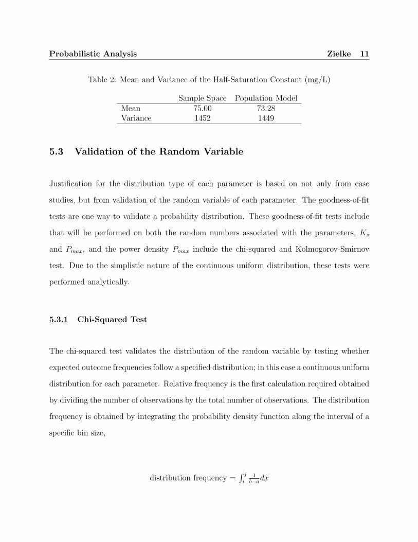
Table 2: Mean and Variance of the Half-Saturation Constant (mg/L)
Sample Space Population ModelMean 75.00 73.28Variance 1452 1449
5.3 Validation of the Random Variable
Justification for the distribution type of each parameter is based on not only from case
studies, but from validation of the random variable of each parameter. The goodness-of-fit
tests are one way to validate a probability distribution. These goodness-of-fit tests include
that will be performed on both the random numbers associated with the parameters, Ks
and Pmax, and the power density Pmax include the chi-squared and Kolmogorov-Smirnov
test. Due to the simplistic nature of the continuous uniform distribution, these tests were
performed analytically.
5.3.1 Chi-Squared Test
The chi-squared test validates the distribution of the random variable by testing whether
expected outcome frequencies follow a specified distribution; in this case a continuous uniform
distribution for each parameter. Relative frequency is the first calculation required obtained
by dividing the number of observations by the total number of observations. The distribution
frequency is obtained by integrating the probability density function along the interval of a
specific bin size,
distribution frequency =∫ j
i1
b−adx
Probabilistic Analysis Zielke 12
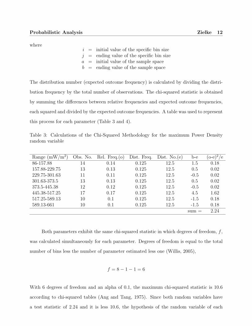
wherei = initial value of the specific bin sizej = ending value of the specific bin sizea = initial value of the sample spaceb = ending value of the sample space
The distribution number (expected outcome frequency) is calculated by dividing the distri-
bution frequency by the total number of observations. The chi-squared statistic is obtained
by summing the differences between relative frequencies and expected outcome frequencies,
each squared and divided by the expected outcome frequencies. A table was used to represent
this process for each parameter (Table 3 and 4).
Table 3: Calculations of the Chi-Squared Methodology for the maximum Power Densityrandom variable
Range (mW/m2) Obs. No. Rel. Freq.(o) Dist. Freq. Dist. No.(e) b-e (o-e)2/e86-157.88 14 0.14 0.125 12.5 1.5 0.18157.88-229.75 13 0.13 0.125 12.5 0.5 0.02229.75-301.63 11 0.11 0.125 12.5 -0.5 0.02301.63-373.5 13 0.13 0.125 12.5 0.5 0.02373.5-445.38 12 0.12 0.125 12.5 -0.5 0.02445.38-517.25 17 0.17 0.125 12.5 4.5 1.62517.25-589.13 10 0.1 0.125 12.5 -1.5 0.18589.13-661 10 0.1 0.125 12.5 -1.5 0.18
sum = 2.24
Both parameters exhibit the same chi-squared statistic in which degrees of freedom, f ,
was calculated simultaneously for each parameter. Degrees of freedom is equal to the total
number of bins less the number of parameter estimated less one (Willis, 2005),
f = 8− 1− 1 = 6
With 6 degrees of freedom and an alpha of 0.1, the maximum chi-squared statistic is 10.6
according to chi-squared tables (Ang and Tang, 1975). Since both random variables have
a test statistic of 2.24 and it is less 10.6, the hypothesis of the random variable of each
Probabilistic Analysis Zielke 13
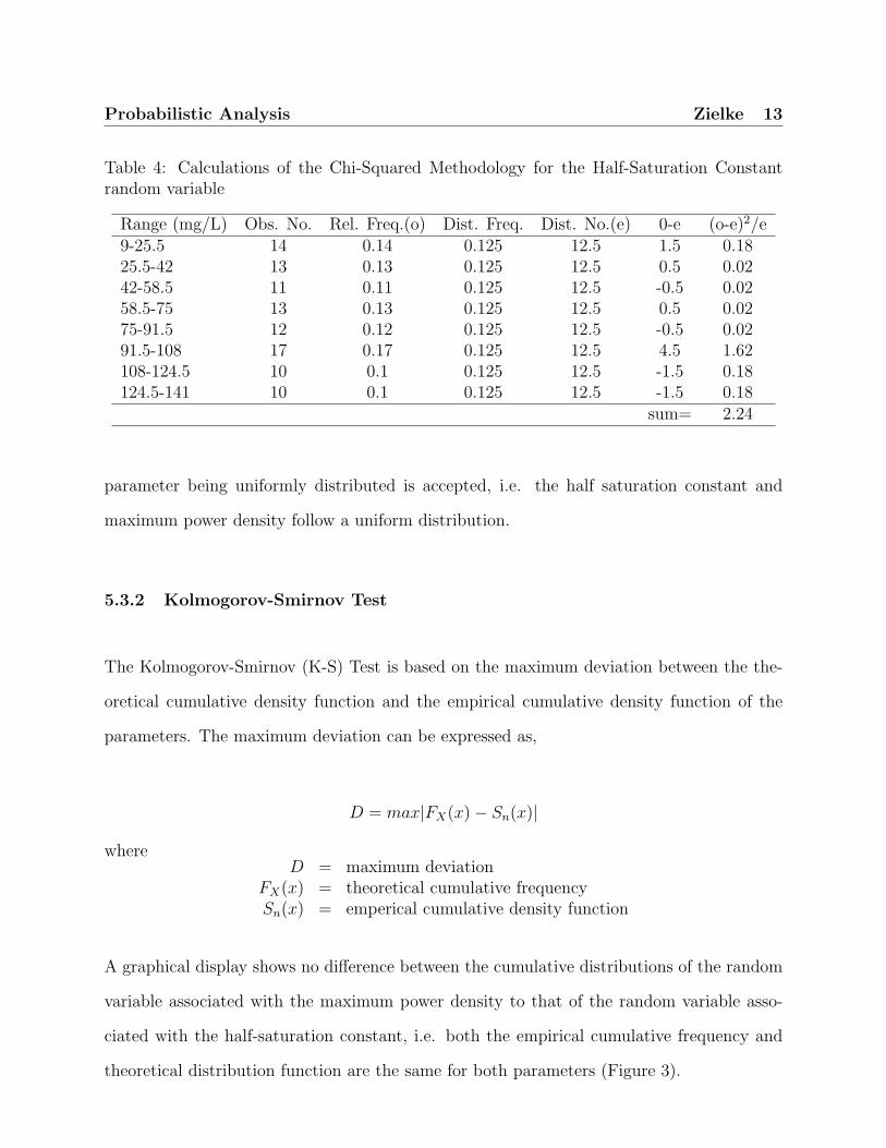
Table 4: Calculations of the Chi-Squared Methodology for the Half-Saturation Constantrandom variable
Range (mg/L) Obs. No. Rel. Freq.(o) Dist. Freq. Dist. No.(e) 0-e (o-e)2/e9-25.5 14 0.14 0.125 12.5 1.5 0.1825.5-42 13 0.13 0.125 12.5 0.5 0.0242-58.5 11 0.11 0.125 12.5 -0.5 0.0258.5-75 13 0.13 0.125 12.5 0.5 0.0275-91.5 12 0.12 0.125 12.5 -0.5 0.0291.5-108 17 0.17 0.125 12.5 4.5 1.62108-124.5 10 0.1 0.125 12.5 -1.5 0.18124.5-141 10 0.1 0.125 12.5 -1.5 0.18
sum= 2.24
parameter being uniformly distributed is accepted, i.e. the half saturation constant and
maximum power density follow a uniform distribution.
5.3.2 Kolmogorov-Smirnov Test
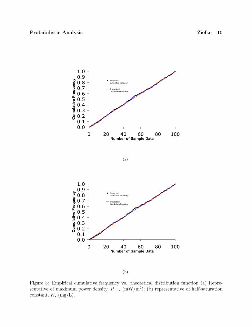
The Kolmogorov-Smirnov (K-S) Test is based on the maximum deviation between the the-
oretical cumulative density function and the empirical cumulative density function of the
parameters. The maximum deviation can be expressed as,
D = max|FX(x)− Sn(x)|
whereD = maximum deviation
FX(x) = theoretical cumulative frequencySn(x) = emperical cumulative density function
A graphical display shows no difference between the cumulative distributions of the random
variable associated with the maximum power density to that of the random variable asso-
ciated with the half-saturation constant, i.e. both the empirical cumulative frequency and
theoretical distribution function are the same for both parameters (Figure 3).
Probabilistic Analysis Zielke 14
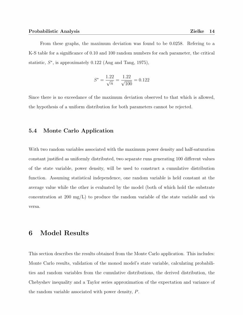
From these graphs, the maximum deviation was found to be 0.0258. Refering to a
K-S table for a significance of 0.10 and 100 random numbers for each parameter, the critical
statistic, S∗, is approximately 0.122 (Ang and Tang, 1975),
S∗ =1.22√
n=
1.22√100
= 0.122
Since there is no exceedance of the maximum deviation observed to that which is allowed,
the hypothesis of a uniform distribution for both parameters cannot be rejected.
5.4 Monte Carlo Application
With two random variables associated with the maximum power density and half-saturation
constant justified as uniformly distributed, two separate runs generating 100 different values
of the state variable, power density, will be used to construct a cumulative distribution
function. Assuming statistical independence, one random variable is held constant at the
average value while the other is evaluated by the model (both of which hold the substrate
concentration at 200 mg/L) to produce the random variable of the state variable and vis
versa.
6 Model Results
This section describes the results obtained from the Monte Carlo application. This includes:
Monte Carlo results, validation of the monod model’s state variable, calculating probabili-
ties and random variables from the cumulative distributions, the derived distribution, the
Chebyshev inequality and a Taylor series approximation of the expectation and variance of
the random variable associated with power density, P .
Probabilistic Analysis Zielke 15
0.00.10.20.30.40.50.60.70.80.91.0
0 20 40 60 80 100Number of Sample Data
Cum
ulat
ive
Freq
uenc
y Empericalcumulative frequency
TheoreticalDistribution Function
(a)
0.00.10.20.30.40.50.60.70.80.91.0
0 20 40 60 80 100Number of Sample Data
Cum
ulat
ive
Freq
uenc
y Empericalcumulative frequency
TheoreticalDistribution Function
(b)
Figure 3: Empirical cumulative frequency vs. theoretical distribution function (a) Repre-sentative of maximum power density, Pmax (mW/m2); (b) representative of half-saturationconstant, Ks (mg/L).
Probabilistic Analysis Zielke 16
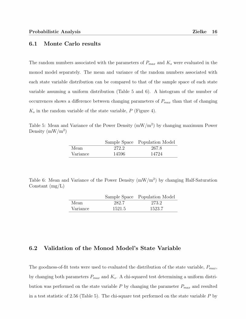
6.1 Monte Carlo results
The random numbers associated with the parameters of Pmax and Ks were evaluated in the
monod model separately. The mean and variance of the random numbers associated with
each state variable distribution can be compared to that of the sample space of each state
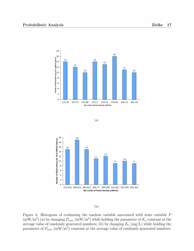
variable assuming a uniform distribution (Table 5 and 6). A histogram of the number of
occurrences shows a difference between changing parameters of Pmax than that of changing
Ks in the random variable of the state variable, P (Figure 4).
Table 5: Mean and Variance of the Power Density (mW/m2) by changing maximum PowerDensity (mW/m2)
Sample Space Population ModelMean 272.2 267.8Variance 14596 14724
Table 6: Mean and Variance of the Power Density (mW/m2) by changing Half-SaturationConstant (mg/L)
Sample Space Population ModelMean 282.7 273.2Variance 1521.5 1523.7
6.2 Validation of the Monod Model’s State Variable
The goodness-of-fit tests were used to evaluated the distribution of the state variable, Pmax,
by changing both parameters Pmax and Ks. A chi-squared test determining a uniform distri-
bution was performed on the state variable P by changing the parameter Pmax and resulted
in a test statistic of 2.56 (Table 5). The chi-square test performed on the state variable P by
Probabilistic Analysis Zielke 17
14
12
10
1413
16
1110
0
2
4
6
8
10
12
14
16
18
115.25 167.57 219.88 272.2 324.51 376.83 429.14 481.45Bin Limits of Power Density (mW/m2)
Num
ber o
f Obs
erva
tions
per
52.
3 m
W/m
2 in
terv
al
(a)
15
19
15
1112
910
9
0
2
4
6
8
10
12
14
16
18
20
232.016 248.914 265.812 282.71 299.609 316.507 333.405 350.303
Bin Limits of Power Density (mW/m2)
Num
ber o
f Obs
erva
tions
per
16.
9 m
W/m
2 in
terv
al
(b)
Figure 4: Histogram of evaluating the random variable associated with state variable P(mW/m2) (a) by changing Pmax (mW/m2) while holding the parameter of Ks constant at theaverage value of randomly generated numbers; (b) by changing Ks (mg/L) while holding theparameter of Pmax (mW/m2) constant at the average value of randomly generated numbers.
Probabilistic Analysis Zielke 18
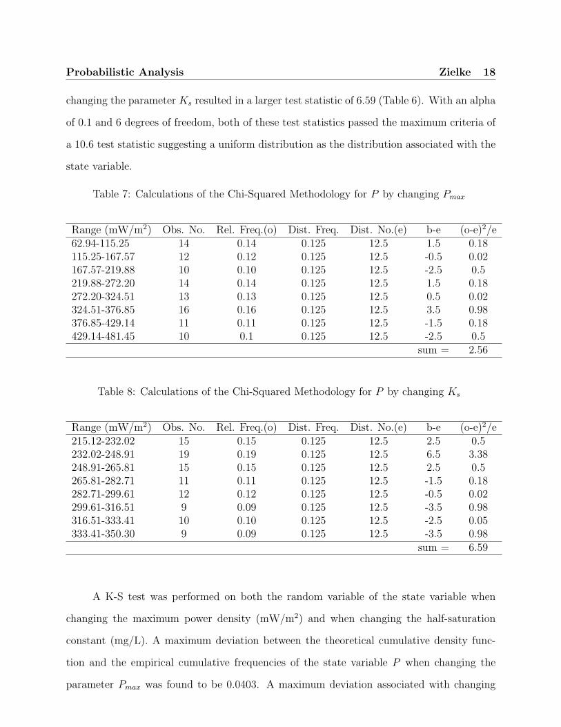
changing the parameter Ks resulted in a larger test statistic of 6.59 (Table 6). With an alpha
of 0.1 and 6 degrees of freedom, both of these test statistics passed the maximum criteria of
a 10.6 test statistic suggesting a uniform distribution as the distribution associated with the
state variable.
Table 7: Calculations of the Chi-Squared Methodology for P by changing Pmax
Range (mW/m2) Obs. No. Rel. Freq.(o) Dist. Freq. Dist. No.(e) b-e (o-e)2/e62.94-115.25 14 0.14 0.125 12.5 1.5 0.18115.25-167.57 12 0.12 0.125 12.5 -0.5 0.02167.57-219.88 10 0.10 0.125 12.5 -2.5 0.5219.88-272.20 14 0.14 0.125 12.5 1.5 0.18272.20-324.51 13 0.13 0.125 12.5 0.5 0.02324.51-376.85 16 0.16 0.125 12.5 3.5 0.98376.85-429.14 11 0.11 0.125 12.5 -1.5 0.18429.14-481.45 10 0.1 0.125 12.5 -2.5 0.5
sum = 2.56
Table 8: Calculations of the Chi-Squared Methodology for P by changing Ks
Range (mW/m2) Obs. No. Rel. Freq.(o) Dist. Freq. Dist. No.(e) b-e (o-e)2/e215.12-232.02 15 0.15 0.125 12.5 2.5 0.5232.02-248.91 19 0.19 0.125 12.5 6.5 3.38248.91-265.81 15 0.15 0.125 12.5 2.5 0.5265.81-282.71 11 0.11 0.125 12.5 -1.5 0.18282.71-299.61 12 0.12 0.125 12.5 -0.5 0.02299.61-316.51 9 0.09 0.125 12.5 -3.5 0.98316.51-333.41 10 0.10 0.125 12.5 -2.5 0.05333.41-350.30 9 0.09 0.125 12.5 -3.5 0.98
sum = 6.59
A K-S test was performed on both the random variable of the state variable when
changing the maximum power density (mW/m2) and when changing the half-saturation
constant (mg/L). A maximum deviation between the theoretical cumulative density func-
tion and the empirical cumulative frequencies of the state variable P when changing the
parameter Pmax was found to be 0.0403. A maximum deviation associated with changing
Probabilistic Analysis Zielke 19
the parameter Ks was found to be 0.0871. Although both these deviations are larger then
the previous deviations found for the random variables associated for the parameters, both of
these deviations associated with the state variable are of lesser value then the critical statistic
of 0.122, i.e. pass the test (Ang and Tang, 1975). Both of these distributions were passed
through a FORTRAN 90 computer program named FA1NEW after compiling the source
code named FA1NEW.f. The results from FA1NEW of the state variable when changing
the maximum power density, Pmax passed both the chi-squared and K-S test for a normal
distribution. For the state variable associated with changing the half-saturation constant,
Ks, FA1NEW results suggested either a Type I Extremal distribution or a Log-Pearson
Type III distribution. Since the uniform distribution is the most simplistic distribution that
passed for both random variables associated with the state variable, the continuous uniform
distribution is chosen as the distribution of power density.
6.3 Calculating Probabilities and Random Variables from the Cu-
mulative Distributions
Both the cumulative frequencies and the cumulative density function can be used to deter-
mine the probability of occurrence of a random variable. They can also be used to determine
a particular probability given a random variable. The examples described in this particular
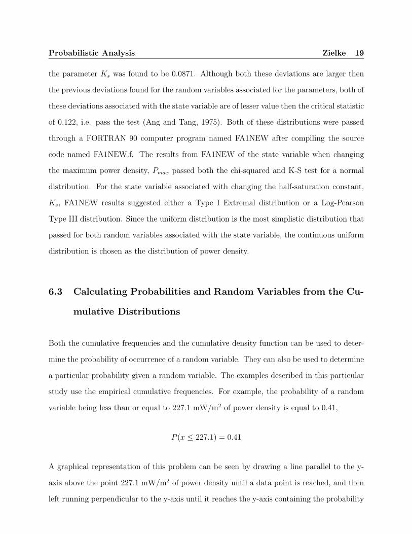
study use the empirical cumulative frequencies. For example, the probability of a random
variable being less than or equal to 227.1 mW/m2 of power density is equal to 0.41,
P (x ≤ 227.1) = 0.41
A graphical representation of this problem can be seen by drawing a line parallel to the y-
axis above the point 227.1 mW/m2 of power density until a data point is reached, and then
left running perpendicular to the y-axis until it reaches the y-axis containing the probability
Probabilistic Analysis Zielke 20
value (Figure 5 (a)). This can also be done in reverse, i.e. given a probability of 0.41, what
is the value of the random variable?
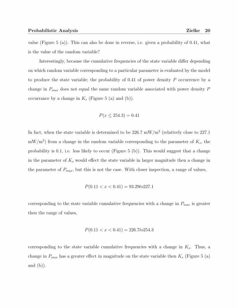
Interestingly, because the cumulative frequencies of the state variable differ depending
on which random variable corresponding to a particular parameter is evaluated by the model
to produce the state variable; the probability of 0.41 of power density P occurrence by a
change in Pmax does not equal the same random variable associated with power density P
occurrance by a change in Ks (Figure 5 (a) and (b)).
P (x ≤ 254.3) = 0.41
In fact, when the state variable is determined to be 226.7 mW/m2 (relatively close to 227.1
mW/m2) from a change in the random variable corresponding to the parameter of Ks, the
probability is 0.1, i.e. less likely to occur (Figure 5 (b)). This would suggest that a change
in the parameter of Ks would effect the state variable in larger magnitude then a change in
the parameter of Pmax, but this is not the case. With closer inspection, a range of values,
P (0.11 < x < 0.41) = 93.29to227.1
corresponding to the state variable cumulative frequencies with a change in Pmax is greater
then the range of values,
P (0.11 < x < 0.41) = 226.7to254.3
corresponding to the state variable cumulative frequencies with a change in Ks. Thus, a
change in Pmax has a greater effect in magnitude on the state variable then Ks (Figure 5 (a)
and (b)).
Probabilistic Analysis Zielke 21
0.41
227.10
0.1
0.2
0.3
0.4
0.5
0.6
0.7
0.8
0.9
1
60 100 140 180 220 260 300 340 380 420 460
Random Variable of Power Density (mW/m2)
Prob
abili
ty o
f Occ
urre
nce
EmpericalCumulativeFrequency
TheoreticalCumulativeDistributionFunction
(a)
0.11
0.41
254.3226.70.0
0.1
0.2
0.3
0.4
0.5
0.6
0.7
0.8
0.9
1.0
200 240 280 320 360
Random Variable of Power Density (mW/m2)
Prob
abili
ty o
f Occ
urre
nce
Emperical CumulativeFrequencyTheoretical CumulativeDensity Function
(b)
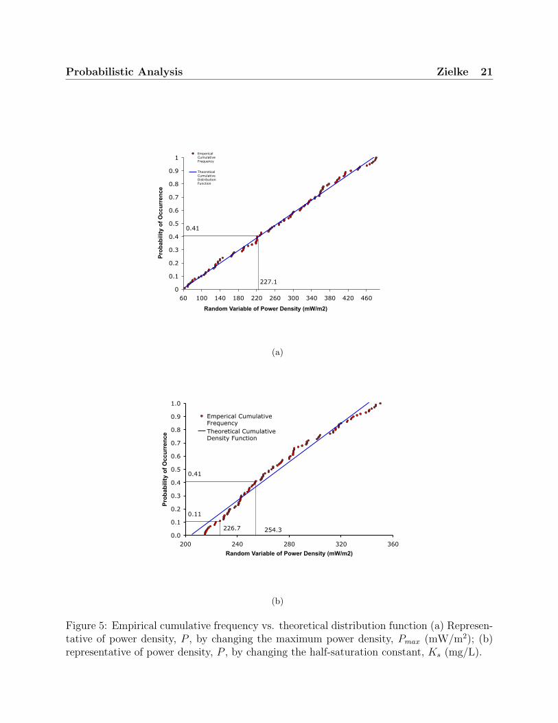
Figure 5: Empirical cumulative frequency vs. theoretical distribution function (a) Represen-tative of power density, P , by changing the maximum power density, Pmax (mW/m2); (b)representative of power density, P , by changing the half-saturation constant, Ks (mg/L).
Probabilistic Analysis Zielke 22
6.4 Derived Probability Distribution
Since the parameter Pmax has the greatest effect on the state variable, it was chosen to be
used as the inverse. The random variable of the state variable, P , associated with a change in
Pmax was determined to have a normal distribution with the computer program FA1NEW so
the parameter can be assumed a normal distributed random variable. The inverse function
of the monod equation can be expressed as,
Pmax =P (Ks + S)
S
The derived density function can then be expressed as,
fP (p) =1√2πσ
e
24− 12
P (Ks+S)
S−µ
σ
!235 (Ks+S)
S
which can be simplified and expressed as,
fP (p) =1√
2πσ S(Ks+S)
e
24− 12
P− S
(Ks+S)µ
σ S(Ks+S)
!235
6.5 Chebyshev inequality
The Chebyshev inequality can show that the mean and standard deviation alone can deter-
mine a probability of a random variable lying within any given bound. The expression can
be denoted as,
P [(mX − hσX) ≤ X ≤ (mX + hσX)] ≥ 1− 1
h2
Probabilistic Analysis Zielke 23
corresponding to one, two and three sigma bounds; h equals 1, 2 and 3. Using P as the
random variable associated with a change in Pmax and with a mean of 267.8 and a standard
deviation of 14724, the expression can be expressed as,
P [(267.8− 14724h) ≤ P ≤ (267.8 + 14724h)] ≥ 1− 1
h2
if h = 2 corresponding to 2 sigma bounds
P [(−29180) ≤ P ≤ (29716)] ≥ 0.75
and assuming non-negativity of power density
P [P ≤ (29716)] ≥ 0.75
In this case, due to the very large magnitude of variance, the bounds are much larger than
the exact bounds. This suggests that the variance associated with the maximum power
density is much larger then what may be thought of as a typical magnitude of variance.
6.6 Taylor Series Approximation
The Taylor series can be used to approximate the mean and variance of the state variable
given empirical data of the state variable. From one case study, twenty seven data points of
the maximum power density correspond to a mean of 356.3 and a variance of 23987 (Lui,
2005). The expected value can then be computed (assuming substrate concentration of 200
mg/L and Ks at the average of the random variable),
E(P ) ' g(µPmax) =356.3 ∗ 200
75 + 200= 259.1
Probabilistic Analysis Zielke 24
The variance can be computed as,
V ar(P ) ' V ar(P )
(dg
dPmax
)2
= V ar(P )S
Ks + S= 23987
200
75 + 200= 17445
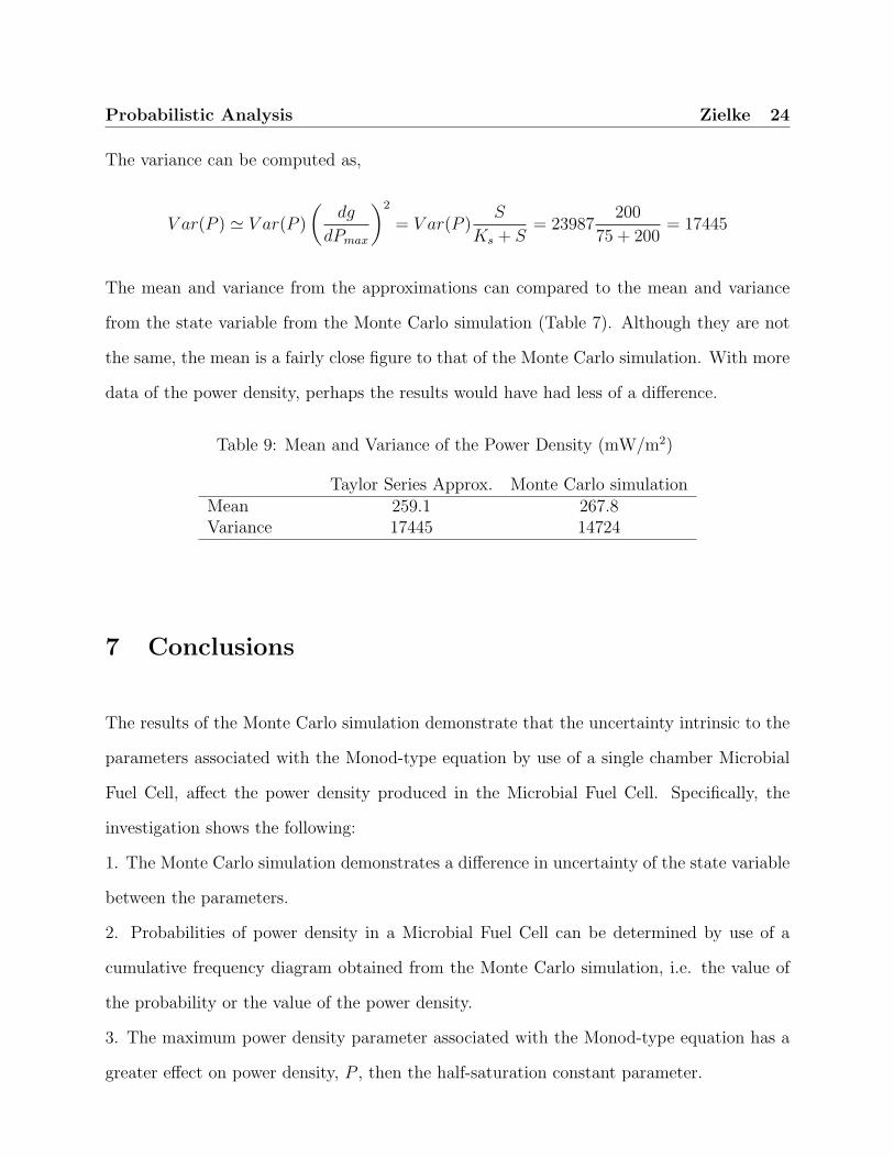
The mean and variance from the approximations can compared to the mean and variance
from the state variable from the Monte Carlo simulation (Table 7). Although they are not
the same, the mean is a fairly close figure to that of the Monte Carlo simulation. With more
data of the power density, perhaps the results would have had less of a difference.
Table 9: Mean and Variance of the Power Density (mW/m2)
Taylor Series Approx. Monte Carlo simulationMean 259.1 267.8Variance 17445 14724
7 Conclusions
The results of the Monte Carlo simulation demonstrate that the uncertainty intrinsic to the
parameters associated with the Monod-type equation by use of a single chamber Microbial
Fuel Cell, affect the power density produced in the Microbial Fuel Cell. Specifically, the
investigation shows the following:
1. The Monte Carlo simulation demonstrates a difference in uncertainty of the state variable
between the parameters.
2. Probabilities of power density in a Microbial Fuel Cell can be determined by use of a
cumulative frequency diagram obtained from the Monte Carlo simulation, i.e. the value of
the probability or the value of the power density.
3. The maximum power density parameter associated with the Monod-type equation has a
greater effect on power density, P , then the half-saturation constant parameter.
Probabilistic Analysis Zielke 25
4. The Taylor series approximation of the mean and variance associated with the power
density is a close approximation to that of the random variable determined in the Monte
Carlo simulation.
5. The variance associated with the maximum power density in a Microbial Fuel Cell is
large.
8 Further Research
There is suspicion as to a joint distribution associated with the parameters in the Monod-type
equation. Further research might show this relationship.
Probabilistic Analysis Zielke 26
9 References
Aiba, S.; Humphrey, A.E.; Millis, N.F.; Biochemical Engineering. Academic Press. NewYork. 1965
Ang, A.H-S; Tang, W. H; Probability Concepts in Engineering Planning and Design JohnWiley and Sons. New York. 1975
Baranyi, J.; Roberts, T.A.; Mathematics of predictive food microbiology. Int. J. Food.Microbiol. 1995, 26, 2, 199-218
Benjamin, J. R.; Cornell, C. A.; Probability, Statistics, and Decision for Civil EngineersMcGraw-Hill. New York. 1970
Dette, H; Melas, B.V.; Pepelyshev, A.; Strigul, N.; Efficient design of experiments in theMonod model. Journal of the Royal Statistical Society: Series B (Statistical Methodolgy),2003, 65, 3, 725-742(18)
Ellis, T.G.; Barbeau, D.S.; Smets, B.F.; Grady Jr, C.P.L.; Respirometric technique fordetermination of extant kinetic parameters describing biodegradation. Water Environ. Res,1996, 68, 5, 917-926
Ferenci, Th.; ”Growth of bacterial cultures” 50 years on: towards an uncertainty princi-ple instead of constants in bacterial growth kinetics. Res. Microbiol. 1999, 150, 7, 431-438
Fu, W; Mathews, A.P.; Lactic acid production from lactose by Lactobacillus plantarum:kinetic model and effects of pH, substrate, and oxygen. Biochem. Eng. J., 3, 3, 163-170
Gottesfeld, S.; Zawodzinski, T.A.; Polymer electrolyte fuel cell. Adv. Electrochem. Sci.1997, 5, 195-301
Liu, C; Zachara, J. M.; Uncertainties of Monod kinetic parameters nonlinearly estimatedfrom batch experiments. Envrion. Sci. Tech. 2001, 35, 133-141
Lui, H.; Cheng, S; Logan, B.E.; Production of Electricity from Acetate or Butyrate Us-ing a Single Chamber Microbial Fuel Cell. Environ. Sci. Tech. 2005, 39, 658-662
Lui, H.; Logan, B.E.; Electricity generation using an air-cathode single chamber micro-bial fuel cell in the presence and absence of a proton exchange membrane. Environ. Sci.Tech. 2004, 38, 4040-4046
Lui, H,; Ramnarayanan, R.; Logan, B.E.; Production of electricity during wastewater treat-ment using a single chamber microbial fuel cell. Environ. Sci. Tech. 2004, 38, 2281-2285
Probabilistic Analysis Zielke 27
Manno, I; Introduction to the Monte-Carlo Method. Akademiai Kiado. Budapist, Hun-gary. 1999
Min, B.; Logan, B.E.; Continuous electricity generation from domestic wastewater and or-ganic substrates in a flat plate microbial fuel cell. Environ. Sci. Tech. 2004, 38, 5809-5814
Monod, J.; The growth of baterial cultures. Ann. Rev. Microbiol., 3, 371-393
Oh, S.; Min, B.; Logan, B.E.; Cathode performance as a factor in electricity generationin Microbial Fuel Cells. Environ. Sci. Technol. 2004, 38, 4900-4904
Schirmer, M; Butler, B.J.; Roy, J.W.; Frind, E.O.; Barker, J.F.; A relative-least-squarestechnique to determine unique Monod kinetic parameters of BTEX compounds using batchexperiments. J. Contam. Hydrol., 1999 37, 1-2, 69-86
Vanrolleghem, P.A.; Spanjers, H.; Petersen, B; Ginestet, Ph.; Takacs, I.; Estimating (com-binations of) activated sludge model no. 1 parameters and components by respirometry.Water Sci. Technol., 1999, 39, 1, 195-214
Willis, R.; Personal Communication. October, 2005.

Probabilistic Analysis Zielke 28
10 Appendix