Proactive Optimal Variable Speed Limit Control for...

Proactive Optimal Variable Speed Limit Control for Recurrently

Congested Freeway Bottlenecks

By

Xianfeng Yang (Corresponding Author)

Ph.D Candidate

Department of Civil & Environmental Engineering

University of Maryland

1173 Glenn L. Martin Hall, College Park, MD 20742

Tel: (301)-405-2638

Email: [email protected]

Yang (Carl) Lu

Ph.D Candidate




Tel: (301)-405-2638


Gang-Len Chang

Ph.D., Professor




Tel: (301)-405-2638


Word Count: 5000 + (9 Figures + 1 table)*250 = 7,500 words

2013 Transportation Research Board 92nd Annual Meeting

Paper #: 13-3139

mailto:[email protected]



Yang, X., Lu, Y., Chang, G.L. 1

ABSTRACT 1

This study presents two models for proactive VSL control on recurrently congested freeway segments. 2

The proposed basic model uses embedded traffic flow relations to predict the evolution of congestion 3

pattern over the projected time horizon, and computes the optimal speed limit. To contend with the 4

difficulty in capturing driver responses to VSL control, this study also proposes an advanced model 5

that further adopts Kalman Filter to enhance the accuracy of traffic state prediction. Both models have 6

been investigated with different traffic conditions and different control objectives. Our extensive 7

simulation analysis with a VISSIM simulator, calibrated with field data from our previous VSL 8

demonstration site, has revealed the benefits of the proposed VSL control model, compared with the 9

case without VSL. Also the results indicated that both proposed proactive models can outperform the 10

basic models and significantly reduce the travel time as well as number of stops over the recurrent 11

bottleneck locations. With respect to several selected MOEs, such as average number of stops and 12

average travel time, it has been found that the one with the control objective of minimizing speed 13

variance clearly outperforms other models. 14


INTRODUCTION 1

VSL is initially designed to reduce the speed difference on some hazardous highway segments, so as 2 to decrease the rear-end collision rate and improve traffic safety (1-3). Recently, it has been 3 recognized that VSL may offer the potential to mitigate traffic congestion and improve traffic 4 efficiency at work-zones and freeway bottlenecks. Through properly displayed and dynamically 5 changed speed limit along a controlled segment, VSL can smooth the transition between the upstream 6 and congested downstream flows to minimize the impact of shockwave on traffic conditions. The 7 mitigation of stop-and-go traffic speed variance can facilitate traffic flows to better utilize the 8 available roadway capacity during peak periods. 9

Despite the potential benefits of VSL for recurrent congestion, design of reliable algorithms 10 to ensure its benefits remains a challenging issue. For example, the Dutch VSL experiment (5) 11 showed no improvement in capacity which may be attributed to its advisory purpose. Bertini (6) 12 analyzed the data obtained from German Autobahn 9 (A9) near Munich, Germany and found strong 13 correlations between the VSL and traffic condition dynamics at bottleneck locations. More recently, 14 Chang et al. (7) reported a successful implementation of an integrated VSL and travel time 15 information system on MD 100 near Coca-Cola Drive which achieved travel time and throughput 16 improvements. 17

Along the same line, a study on the I-495 Capital Beltway (8) revealed that VSL can delay 18 the formation of bottleneck congestion. Abdel-Aty et al. (9, 10) developed a VSL system for I-4 19 through Orlando, Florida and reported to reduce both crash risk and travel time under a simulated 20 environment. Hegyi et al. (11, 12) modified the METANET macroscopic traffic flow model to 21 incorporate the VSL effect and adopted the model predictive control (MPC) approach to determine 22 the optimal speed limit. Papageorgiou et al. (13) and Carlson et al. (14) analyzed the effect of VSL on 23 aggregated traffic flow behavior from the theoretical perspective, and proposed an open-loop 24 integrated optimal control framework to coordinate ramp metering with VSL control. Their 25 simulation results show a reduction of 15 percent in total travel time. Most recently, Hadiuzzaman et 26 al. (15) proposed a modified CTM based VSL control and also used the model predictive control 27 (MPC) method to dynamically change the speed limit in real time. Their VISSIM simulation results 28 showed a reduction of 15-17 percent in travel time and flow rate. 29

In brief, most reactive control algorithms reported in the literature show some difficulty in 30 improving the traffic flow efficiency, while most proactive models seem to yield better control results. 31 Hence, further exploration of the proactive VSL control will be essential for its effective 32 implementation on recurrently congested highway segments. Some priority research issues to be 33 addressed include the effect of prediction accuracy of traffic conditions on a VSL’s effectiveness, and 34 the best control objective to maximize the operational efficiency. This study proposed two types of 35 VSL model in response to these issues: a basic model based on the modified macroscopic traffic flow 36 model (16, 17), and an advanced model with its prediction function enhanced by Kalman Filter. Each 37 VSL model has been tested with two control objectives: total travel time minimization and speed 38 variance minimization. 39

This paper is organized as follows: The key features of the proposed VSL system are briefly 40 described in the next section. Formulations of the basic proactive are introduced in Section 3. Section 41 4 addresses the design of the traffic state estimator, based on the Kalman filtering methodology, 42 followed by presentation of the enhanced VSL model. Design of simulation experiments for 43 evaluating the performance of our proposed models under simulated real-time control environments is 44 reported in Section 6. Conclusions and future research are summarized in the last section. 45


VSL SYSTEM DESCRIPTION 1

As shown in FIGURE 1, due to the perceived congestion the upstream approaching vehicles are often 2

forced to slow down before reaching the bottleneck. The formation of bottleneck may be caused by 3

various factors such as lanes reduction or weaving maneuvers from heavy off-ramp flows. Without 4

proper control, the approaching vehicles are likely to slow their speeds abruptly just upstream of the 5

bottleneck location, often dropping from a “free-flow” to “stop-and-go” conditions and consequently 6

producing shockwaves to reduce the throughput as well as the speed over the bottleneck segment. The 7

VSL proposed in this study is designed to mitigate such shockwave impacts and to best use the 8

available roadway capacity of the congested segment. 9

Bottleneck

On-ramp

Off-rampDetectors

VSL VSL

Flow Direction

10

FIGURE 1 Configuration of a VSL system 11

The proposed VSL system consists of detectors, variable speed limit signs, and a central 12 processing unit to execute control actions. For a target freeway stretch, the upstream detector is used 13 to capture the free-flow arrival rate, and a downstream detector is designed to record the discharging 14 rate from the bottleneck. Also, additional detectors are placed at those on-ramps and off-ramps to 15 record ramp arriving and departing flows. Several VSL signs along with detectors would be installed 16 between the upstream and downstream detectors. In a field application, those VSL signs will 17 dynamically update their displayed speed limit based on the computed optimal set of speeds and the 18 specified criteria for VMS display. 19

Depending on the approaching volume, driver compliance rate, and the resulting congestion 20 along the target freeway segment, a VSL system’s central processing unit is responsible to produce 21 the time-varying optimal speed limits. Note that for the safety concern and effective communications 22 with drivers, all displayed speed limits are supposed to remain unchanged over the length of T

C 23

seconds. 24

BASIC PROACTIVE CONTROL MODEL 25

The operational structure of the proposed VSL control system includes the following two principal 26

components: 27

Macroscopic Traffic Flow Model: Given the detected upstream flow rate and downstream 28

discharging rate, the traffic flow model is used to predict the traffic state evolution in each freeway 29

subsection; 30

Optimization model: Based on the predicted conditions from traffic flow model, the optimization 31

model is adopted to find the optimal set of speed limits with respect to a specified objective 32

function. 33


For convenience of discussion, the control variables and parameters are listed below: 1

Control time and subsection index 2

- ΔT: Unit time interval for control operations; 3

- TP: Time interval for prediction horizon; 4

- TC: Time interval for control horizon; 5

- k: Time interval index for control operation; 6

Network geometric and physical data 7

- Δl: Length of each freeway segment; 8

- ni: Number of lanes in subsection i; 9

Traffic states 10

- qi(k): Transition flow rate entering segment (i-1) from segment i during interval k; 11

- ri(k): On-ramp flow rate entering segment i during interval k; 12

- si(k): Off-ramp flow rate entering segment i during interval k; 13

- Qi(k): Average flow rate in segment i during interval k; 14

- di(k): Mean traffic density in segment i during interval k; 15

- ui(k): Mean speed in segment i during interval k; 16

Control variables and boudaries 17

- vi(k): Variable speed limit ratio in segment i during interval k; 18

- dJ: Jam traffic density; 19

- uJ: Minimum mean speed; 20

- dc: Critical traffic density; 21

- uf(k): Free flow speed; 22

Model Parameters 23

- αi: Transition flow weigh factor; 24

- βi, γ: Speed-density adjustment factor; 25

- ν, τ, κ: Traffic state model parameter. 26

Macroscopic Traffic Flow Model 27

To perform a proactive dynamic VSL control, a reliable prediction model is essential to predict the 28

traffic state evolution under the detected traffic conditions and driver responses. This study employs a 29

calibrated traffic flow model to predict traffic conditions over the target time horizon and to provide 30

the essential information for the VSL optimization module. 31

VSL1 VSL2

Qf(k)

Uf(k)Qi(k)

ui(k)

di(k)

12...ii+1N

qi(k)Qb(k)

Ub(k)

0

32

FIGURE 2 Typical freeway segments 33


As shown in FIGURE 2, for convenience of computation, the target freeway segment is 1 divided into N subsections with a unit length of Δl. While dividing a freeway segment into 2 subsections, the length of subsections should be sufficiently long so that vehicles cannot pass one 3 subsection during one time interval k. Moreover, each subsection is allowed to have at most one on-4 ramp and one off-ramp. For each subsection i, the mean density, di(k), can be determined by the 5 difference between the input and output flows as follows: 6

1( ) ( 1) [ ( ) ( ) ( ) ( )]*

i i i i i i

i

Td k d k q k q k r k s k

l n

(1) 7

The transition flow rate is determined by the mean speed, density, the capacity of target 8 segment, and the remaining capacity of the downstream segment, that is: 9

1 max 1( ) { ( ) (1 ) ( ), , ( ( )) }i i i i i i J i iq k Min Q k Q k q n d d k n (2) 10

where, αi (transition flow weight factor) can be calibrated with field measurements. Wu and 11 Chang (17) stated that it should lie in the interval [0.5,1.0]. 12

For the average speed, ui(k), one can also establish its evolution relation with the following 13 properly selected speed-density relation and shock-wave formation equations: 14

( ) ( 1) { [ ( 1)] ( 1)} ( 1)i i i i i iu k u k S d k u k g k (3) 15

The second component describes an adaptation of the average speed to the speed-density 16 characteristics, as: 17

if ( )

( 1)[ ( ), ( )] ( )

if ( )

( 1)

f

i i c

J

i i f ii i c

J

c

u d k d

d

S d k v k d ku d k d

d

d

(4) 18

Eq.(4) was originally formulated by Hadiuzzaman (15); and the third component gi(k) of 19 Eq.(3) takes into account the density difference between downstream and upstream segments (18), 20 that is: 21

( 1, ) ( , )( )

( , )i

v T d i k d i kg k

l d i k

(5) 22

Constraints 23

In a field application, drivers may begin to reduce the speed when they perceive the VSL sign. 24

Therefore, assuming a driver’s perception distance to be Δl, the target controlled area shall start from 25

one segment ahead of the VSL location (e.g., as shown In FIGURE 2, the controlled area with VSL-2 26

includes segment 0 to segment 3; the controlled sections with VSL-1 are segment 4 to segment i+1). 27

For each subsection i, the mean speed shall be constrained by: 28


( ) , segment i without VSL control;

( ) (k), segment i with VSL control.

J i f

J i f i

u u k u

u u k u v

(6) 1

And, 2

0 (k) 1iv (7) 3

In view of the jam density, one shall also set the density boundaries as follows: 4

0 ( )i Jd k d (8) 5

Also, for safety concern the speed variation between consecutive intervals is set to be within 6 the following boundaries. 7

( ) ( 1)f f

i i i iu v k u v k (9) 8

where, δ is the maximum allowable difference between two successive speed displays on 9 VMS. 10

Objective Functions 11

As the primary focus of VSL is to increase traffic flow speed and its stability, this study first adopts 12

the following minimization of total travel time over the controlled segment as the objective function: 13

min ( )i i

k i

n d k T (10) 14

Note that depending on the response of drivers to the displayed speeds, the embedded 15 macroscopic traffic flow models and the above objective function may not fully capture the complex 16 traffic dynamics and yield the true optimal results. 17

Some existing studies report that a proper VSL control can help smooth speed transition, 18 which will consequently reduce the number of vehicle stops and shockwave impact on the traffic 19 conditions (7). Hence, this study has further explored the following objective function of minimizing 20 the speed variance along the target freeway for a VSL control: 21

2min ( ( ) )i ave

k i

u k u (11) 22

where, uave is the average speed of the target freeway stretch, and is given as follows: 23

( )

( / )

i

k iave c

u k

uT T N

(12) 24


For safety concern the speed variation between consecutive intervals is limited within a given 1

range, as Shown in Eq. (9). Therefore, the feasible solution set is quite small and one can thus adopt 2

enumerative search for the optimal solution. 3

ENHANCED PROACTIVE CONTROL MODEL 4

To fully capture the complex interrelations between speed and density, this study has further adopted 5

the Kalman Filter to improve the accuracy of the predicted traffic conditions over the target time 6

horizon for proactive VSL control. The Kalman Filter is an optimal state estimator applied to a 7

dynamic system that involves random noise and includes a limited amount of noisy real-time 8

measurements. The correction and update process of a typical Kalman Filter process is summarized in 9

FIGURE 3: 10

ŷ-(k) = Ay(k-1) + Bu(k)

(priori estimate state)

P-(k) = AP(k-1)AT + Q

(priori estimate error covariance

Prediction (Time Update)

(1) Project the state ahead

(2) Project the error covariance ahead

Correction (Measurement Update)

(1) Compute the Kalman Gain

(2) Update estimate with measurement zk

(3) Update Error Covariance

ŷ(k) = ŷ-(k) + K(z(k) - H ŷ-(k) )

(posterior estimate state)

K = P-(k)HT(HP-(k)HT + R)-1

(Blending factor)

P(k) = (I - KH)P-(k)

(posterior estimate error covariance)

11

FIGURE 3 An Illustration of Kalman Filter Correction and Update Process 12

where, y(k) is the estimated traffic state vector, and u(k) is the system input: 13

1 1 2 2

0 0 1 1 1 1

[ ( ) ( ) ( ) ( ) ( ) ( ) ]

[ ( ) ( ) ( ) ( ) ( ) ( ) ( ) ( )]

T

N N

T

N N N N

k q k u k q k u k q k u k

k q k v k q k v k r k r k s k s k

y( )

u( ) 14

z(k) is the vector of measurement, and has the following relation with y(k): 15

k k kz( ) = Hy( ) + v( ) (14) 16

where, v(k) is the measurement error. 17

By using Kalman Filter, the predicted traffic state can be constantly updated based on the 18 detector data, and the new optimal speed limits can then be generated with the proposed optimization 19 model. 20


As mentioned in Section 2, to prevent confusing drivers, the displayed speed limits are not 1 allowed to change frequently. Therefore, by defining a control horizon T

C, the speed limits will 2

remain unchanged over the specified time interval. Also note that the optimization model will be 3 activated once all detector data have been updated, where the control horizon is normally equal to the 4 length of multiple detector update intervals. Therefore, during each control horizon, the optimization 5 model will produce multiple estimates of the optimal speed limit, and the process to select the robust 6 one prior to its execution is shown below. 7

For example, assuming that he VSL’s display interval (control horizon) is set as 5 minutes 8 and the detector data is updated at every 1 minute, then each control interval will have five sets of 9 estimated optimal speed limits prior to its implementation time, as shown in FIGURE 4. 10

Time(min)k k+1 k+5 k+10

1st Iteration

Opt. v(1)

A new Speed will be

displayed

2nd

Iteration

3rd

Iteration

4th Iteration

5th Iteration

Opt. v(2)

Opt. v(3)

Opt. v(4)

Opt. v(5)

KF

KF

KF

KF

KF

11

FIGURE 4 An example of the VSL control Strategy 12

Given the set of computed optimal speed limits for the same horizon, {v(1),v(2),…,v(n)}, one 13 can determine the speed limits to be displayed based on the following procedure as used in most 14 online systems (19): 15

1) Define a counter M to identify the moving direction of the speed limit, and then denote vt as the 16

displayed speed limit of the current horizon, where M is updated by the following expression: 17

1, if v(i)>v

, if v(i)=v , i=1,2, n;

1, if v(i)<v

t

t

t

M

M M

M

(15) 18

2) The new displayed speed limit for the next horizon will be readjusted with the predetermined 19

increment Δ, based on the value of M: 20

1

, if M>0

, if M=0

, if M<0

t

t t

t

v

v v

v

(16) 21


In summary, the entire proactive control process includes the following primary steps: 1

Step 0: Divide the target freeway segment into a set of subsections and then deploy the VSL signs and 2 detectors; determine the length of control time interval. 3

Step 1: Apply the Kalman Filter module to revise the predicted traffic conditions produced from the 4 macroscopic traffic model, and execute the optimization model to generate a new set of 5 optimal speed limits for each detector data update interval. 6

Step 2: Update the counter M by comparing the new optimal speed limit with the current displayed 7 speed, (see Eq.(15)). 8

Step 3: Select the new speed limits to display, based on Eq.(16). 9 Step 4: Stop the VSL operations if traffic flow speed has evolved back to its normal prevailing speed. 10

The operational flow chart of the VSL control system is presented in FIGURE 5: 11

Freeway Segmentation

Locate VSL and Detectors

Traffic Flow

Model

Optimization

Model

Kalman Filter

correction

update

Initialization

t=0, M=0

Detector Data

t = t+1

Counter M

update

t < Tc ?

Control

Strategy

Display new

speed limit

Stop VSL?

Stop

Yes

No

No

Yes

Start

12

FIGURE 5 Flow chart of the enhanced proactive model VSL control system 13

SYSTEM EVALUATION 14

Case Description 15

To evaluate the proposed optimization models, this study selected the segment MD-100 West from 16

MD 713 to Coca-Cola Drive, our previous VSL field demonstration site, for simulation analysis. On 17

typical weekdays, the speed during the peak hours usually drops quickly from 60 to 20 mph (e.g., in 5 18

mins) after the onset of congestion, and recovers to about 40 mph after passing Coca-Cola Drive. 19


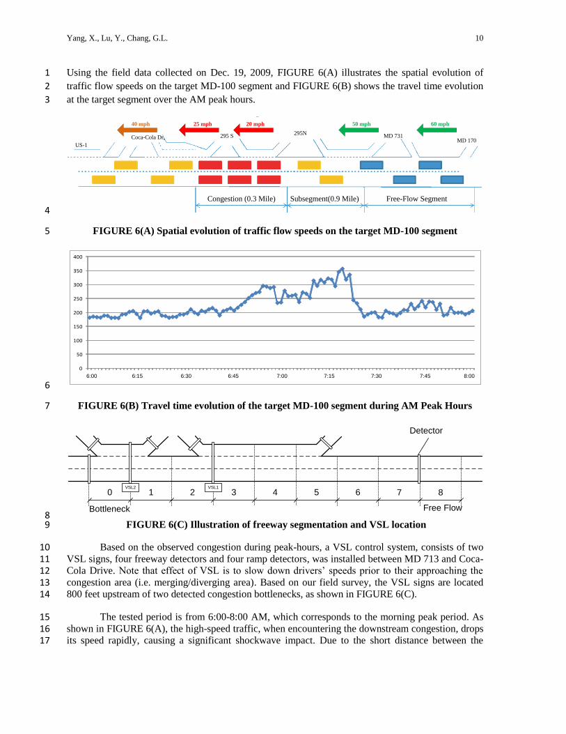
Using the field data collected on Dec. 19, 2009, FIGURE 6(A) illustrates the spatial evolution of 1

traffic flow speeds on the target MD-100 segment and FIGURE 6(B) shows the travel time evolution 2

at the target segment over the AM peak hours. 3

MD 170MD 731

295N295 SCoca-Cola Dr,

US-1

Congestion (0.3 Mile) Subsegment(0.9 Mile) Free-Flow Segment

20 mph25 mph40 mph 50 mph 60 mph

4

FIGURE 6(A) Spatial evolution of traffic flow speeds on the target MD-100 segment 5

0

50

100

150

200

250

300

350

400

1 3 5 7 9 11

13

15

17

19

21

23

25

27

29

31

33

35

37

39

41

43

45

47

49

51

53

55

57

59

61

63

65

67

69

71

73

75

77

79

81

83

85

87

89

91

93

95

97

99

10

1

10

3

10

5

10

7

6:00 6:15 6:30 6:45 7:00 7:15 7:30 7:45 8:00

6

FIGURE 6(B) Travel time evolution of the target MD-100 segment during AM Peak Hours 7

0 1 2 3 4 5 6 7 8VSL2 VSL1

Detector

Bottleneck Free Flow8

FIGURE 6(C) Illustration of freeway segmentation and VSL location 9

Based on the observed congestion during peak-hours, a VSL control system, consists of two 10 VSL signs, four freeway detectors and four ramp detectors, was installed between MD 713 and Coca-11 Cola Drive. Note that effect of VSL is to slow down drivers’ speeds prior to their approaching the 12 congestion area (i.e. merging/diverging area). Based on our field survey, the VSL signs are located 13 800 feet upstream of two detected congestion bottlenecks, as shown in FIGURE 6(C). 14

The tested period is from 6:00-8:00 AM, which corresponds to the morning peak period. As 15 shown in FIGURE 6(A), the high-speed traffic, when encountering the downstream congestion, drops 16 its speed rapidly, causing a significant shockwave impact. Due to the short distance between the 17


diverging (295N off-ramp) and merging (295N on ramp) points, the congestion compounded with 1 weaving activities has resulted in a large capacity reduction at the bottleneck subsection. 2

To create a more congested downstream bottleneck for better evaluation of proposed models, 3 the tested traffic flow pattern is adjusted according to the filed data. As shown in FIGURE 7, around 4 55 percent of traffic flows come from the upstream segment and the rest are from the MD 713 and 5 295 N on-ramp. Also, about 15 percent of the approaching flows take the route via bottleneck 6 segment to the 295 S off-ramp, and the remaining 85 percent flows enter the downstream freeway. 7

1000

1400

18002000

2500

2800 2800 28002600

2400 23002200

0

500

1000

1500

2000

2500

3000

6:15 6:30 6:37 6:45 6:52 7:00 7:07 7:15 7:22 7:30 7:45 8:00

Upstream flow in

FIGURE 7(A) Time-varying approaching flows

from upstream segment

400500

600

800

1000

1300 13001200

1100

900800

500

0

200

400

600

800

1000

1200

1400

6:15 6:30 6:37 6:45 6:52 7:00 7:07 7:15 7:22 7:30 7:45 8:00

MD 713 flow in

FIGURE 7(B) Time-varying approaching flows

from MD 713

500600

800

10001100

1350 1350 14001300

1100

900

700

0

200

400

600

800

1000

1200

1400

1600

6:15 6:30 6:37 6:45 6:52 7:00 7:07 7:15 7:22 7:30 7:45 8:00

295 N flow in

FIGURE 7(C) Time-varying approaching flows

from 295 N on-ramp

263

368

474 526

658

737 737 737 684

632 605 579

0

100

200

300

400

500

600

700

800

6:15 6:30 6:37 6:45 6:52 7:00 7:07 7:15 7:22 7:30 7:45 8:00

295 N flow out

FIGURE 7(D) Time-varying leaving flows via 295

N off-ramp

Design of Simulation Tests and Parameter Selection 8

For performance evaluation, the micro-simulation software VISSIM, with its key parameters 9

calibrated with data collected from our previous field study (7), is used as an unbiased platform. On 10

the selected freeway segment (see FIGURE 6), our research group implemented two VSL signs, four 11

sensors along with License-plate-recognition (LPR) system on Dec. 2009- Jan 2010. With the sensor 12

data and real travel time information from the LPR, the calibration objective is to minimize the 13

difference between simulated travel time and real travel time along the target freeway segment. For 14

the car-following parameters, the max look ahead distance was calibrated to be 1000 ft, and the CC1 15

(headway time) was set as 0.80 s. Lane-changing parameters were also calibrated: the maximum 16

deceleration is -20.11 ft/s2 for own and -19.85 ft/s

2 for trailing vehicle; the accepted deceleration is -17

8.27 ft/s2 and -6.63 ft/s

2 for own and trailing vehicle respectively; the waiting time before diffusion is 18

90 s. 19


To simulate the on-line VSL control with our proactive algorithms, this study has developed a 1

VB.NET program to capture the online interaction between execution of the control algorithm and the 2

time-varying traffic conditions. This mechanism has been programmed to enable our developed 3

optimal VSL module to communicate with VISSIM during every simulation interval. Also note that 4

the compliance rate of VSL is assumed to be 100% in this study. 5

To compare the proposed VSL models with No-control scenario, this study has designed the 6 following four scenarios: 7

Scenario-1: the basic proactive model with the objective of total travel time minimization; 8

Scenario-2: the enhanced proactive model with the objective of total travel time minimization; 9

Scenario-3: the basic proactive model with the objective of speed variance minimization; and 10

Scenario-4: the enhanced proactive model with the objective of speed variance minimization. 11

The key model parameters for the experimental analysis are set as follows: 12

The transition flow weigh factor αi is 0.95; 13

The Speed density adjustment factor βi is 0.8; 14

The congestion wave speed γ is 25 km/h; 15

The Jam traffic density is 100 veh/lane/km; 16

The Critical traffic density is 35 veh/lane/km; 17

The free flow speed is 100 km/h; 18

The allowed speed limit variance δ between two adjacent interval is 10 km/h; 19

Parameter ν, τ, κ, calibrated by Wang (18), are 35 km/h, 20s and 13 veh/lane/km, respectively. 20 Note that we full recognize the need to calibrate these parameters in field applications. However, this 21 study presents our work at the exploratory stage, not for final model and for field application. Hence, 22 our proposed model has directly taken the values of those parameters from the literature. Also, please 23 note that those parameters adopted from the literature serve only as the initial values of the KF 24 updating process, and thus its impact on the prediction results will be diminished over time when 25 more and more data are detected from traffic sensors. 26

In the Kalman Filter model, the deviation of measurement errors for the flow rate and speed 27 are selected from an extensive analysis of the experimental results and field data: 28

( ( )) 50 veh/h, ( ( )) 50 veh/h, ( ( )) 50 veh/h;

( ( )) 5 km/h;

q q q

i i i

u

i

D k D r k D s k

D k

29

The deviation of prediction errors for the flow rate and speed are assumed to be: 30

( ( )) 250 veh/h, ( ( )) 10 km/hq u

i iD k D k 31

Analysis of Experimental Results 32

Based on the objective of minimizing the total travel time, FIGURE 8(A) shows the distribution of 33

mean speeds at the bottleneck segment-0 under Scenario-1, Scenario-2, and No-control scenario, 34

revealing that the speeds under different scenarios are identical during the first hour (6:00-7:00AM) 35


due to the light traffic condition. However, during the peak hour (7:00-8:00AM), the traffic demands 1

increase significantly and result in the downstream congestion. Comparing these three scenarios, it is 2

clear that Scenario-2 can offer a higher speed (20 km/h) at the beginning of the congestion period 3

(7:10-7:15AM), and maintain a more stable speed over the rest period (7:15-8:00AM) compared to 4

the No-VSL control scenario. However, Scenario-1 (without update by the Kalman Filter method) 5

fails to provide a proper control during the whole control period, which is due likely to its deficiency 6

in offering an accurate traffic prediction and consequently unable to generate effective control speeds. 7

On contrast, FIGURE 8(B) represents mean speed evolution of the scenarios with the control 8 objective of minimizing speed variance at the bottleneck. Obviously, Scenario-4 is able to maintain a 9 stable bottleneck speed, starting from beginning of the traffic congestion period (7:00-8:00AM). Also, 10 it can help reduced the congested duration, based on the speed evolution over the period (7:55-11 8:00AM). Scenario-3 can also offer acceptable control results. Compared with the No-Control 12 scenario, the basic model was able to keep a higher speed at the beginning of congestion period (7:08-13 7:15AM), but lost its efficiency during the remaining period, as shown in FIGURE 8(B). The reason, 14 as stated previously, is that the basic model is unable to capture the rapidly changing traffic condition 15 and to revise the speed limit in time during the on-line applications. 16

Among all scenarios, the KF models with their proactive nature can always outperform the 17 Basic models. Therefore, this study has further investigated the properties of these two KF models 18 with different objective functions, and the results are shown in FIGURE 8(C). 19

0

20

40

60

80

100

120

6: 00 6: 15 6: 30 6: 45 7: 00 7: 15 7: 30 7 : 8

No-VSL Scenario-1 Scenario-2

6:00 6:15 6:30 6:45 7:00 7:15 7:30 7:45 8:00

Time

Sp

ee

d (

km

/h)

20

FIGURE 8(A) Mean speed at segment 0: Scenario 1,2 v.s. No-VSL scenario 21

0

20

40

60

80

100

120

6: 00 6: 15 6: 30 6: 45 7: 00 7: 15 7: 30 7 : 8


Sp

ee

d (

km

/h)

6:00 6:15 6:30 6:45 7:00 7:15 7:30 7:45 8:00

Time

22


FIGURE 8(B) Mean speed at segment 0: Scenario 3,4 v.s. No-VSL scenario 1

0

20

40

60

80

100

120

6: 00 6: 15 6: 30 6: 45 7: 00 7: 15 7: 30 7 : 8


Sp

ee

d (

km

/h)

6:00 6:15 6:30 6:45 7:00 7:15 7:30 7:45 8:00

Time

2

FIGURE 8(C) Mean speed at segment 0: Scenario 2,4 v.s. No-VSL scenario 3

As a major MOE to evaluate traffic efficiency, the time-dependant travel time can clearly 4 reflect the effectiveness of each control strategy. FIGURE 9(A) presents the resulting travel time from 5 these two models with the objective of minimizing travel time and the No-VSL scenario. Notably, the 6 travel time starts to increase when the freeway is becoming congested (after 7:00AM). Compared 7 with the No-control scenario, the average travel time is reduced by 70 seconds in Scenario-2, 8 demonstrating the benefits under the VSL control. From FIGURE 9(B), it is clear that both speed-9 variance minimization models can reduce the travel time during the congested period (7:00-8:00AM). 10 Also, the KF based model in Scenario-4 clearly outperforms the basic model in Scenario-3. 11

A further comparison between two KF models is shown in FIGURE 9(C). Note that during 12 the period 6:45~7:00AM, Scenario-2 with the travel time minimization objective produces a lower 13 travel time (20 secs on average) than Scenario-4 of minimizing the speed variance. However, as the 14 congestion increases from 7:15AM, Scenario-4 begins to show better performance. To understand the 15 reason of this interesting finding, we further analyzed the simulation process and found out that the 16 variance-minimization model in Scenario-4 is more sensitive to the change in traffic conditions 17 because it can immediately adjust the speed limit in advance even during the moderate congested 18 period. The capability to sensitively adjust speed control in time can reduce the flow rate to the 19 downstream segments, and consequently mitigate the potential shockwave impact. 20

0

100

200

300

400

500

600

6 : 0 0 6 : 1 5 6 : 3 0 6 : 4 5 7


6:00 6:15 6:30 6:45 7:00 7:15 7:30 7:45 8:00

Time

Me

an

Tra

ve

l T

ime

(se

cs)

21

FIGURE 9(A) Time-dependent travel time: Scenario 1,2 v.s. No-VSL scenario 22


0

50

100

150

200

250

300

350

400

450

500

6 : 0 0 6 : 1 5 6 : 3 0 6 : 4 5 7


6:00 6:15 6:30 6:45 7:00 7:15 7:30 7:45 8:00

Time

Me

an

Tra

ve

l T

ime

(se

cs)

1

FIGURE 9(B) Time-dependent travel time: Scenario 3,4 v.s. No-VSL scenario 2

0

50

100

150

200

250

300

350

400

450

500

6 : 0 0 6 : 1 5 6 : 3 0 6 : 4 5 7


6:00 6:15 6:30 6:45 7:00 7:15 7:30 7:45 8:00

Time

Me

an

Tra

ve

l T

ime

(se

cs)

3

FIGURE 9(C) Time-dependent travel time: Scenario 2,4 v.s. No-VSL scenario 4

0

5

10

15

20

25

6 : 0 0 6 : 1 5 6 : 3 0 6 : 4 5 7


6:00 6:15 6:30 6:45 7:00 7:15 7:30 7:45 8:00

Time

Ave

. n

um

be

r o

f S

top

s

5

FIGURE 9(D) Time-dependent # of stops: Scenario 1,2 v.s. No-VSL scenario 6


0

5

10

15

20

25

6 : 0 0 6 : 1 5 6 : 3 0 6 : 4 5 7


6:00 6:15 6:30 6:45 7:00 7:15 7:30 7:45 8:00

Time

Ave

. n

um

be

r o

f S

top

s

1

FIGURE 9(E) Time-dependent # of stops: Scenario 3,4 v.s. No-VSL scenario 2

0

5

10

15

20

25

6 : 0 0 6 : 1 5 6 : 3 0 6 : 4 5 7


6:00 6:15 6:30 6:45 7:00 7:15 7:30 7:45 8:00

Time

Ave

. n

um

be

r o

f S

top

s

3

FIGURE 9(F) Time-dependent # of stops: Scenario 2,4 v.s. No-VSL scenario 4

As reported in the literature, an effective VSL system can reduce a driver’s “stop-and-go” 5 frequency. Therefore, the number of vehicle stops can also be viewed as an effective MOE for 6 evaluating the efficiency of each proposed VSL system. FIGURE 9(D) ~ 9(F) also compare the time-7 dependent number of vehicle stops among different scenarios, and the results also indicate the 8 promising property of the KF models, especially the one with the objective of minimizing speed 9 variance (Scenario-4). 10

TABLE 1 summarizes the MOEs for all scenarios. To prevent the randomness of results, the 11 data have been averaged over 10 simulation replications. Moreover, to distinguish the performance 12 between the congested (7:00-8:00AM) and uncongested periods (6:00-7:00AM), TABLE 1 shows the 13 overall results over the entire period and over the congested period. Notably, all three effective modes 14 can yield significant reduction in both total travel time and vehicle stops. Among those three, 15 Scenario-4 is the best one which yielded a reduction of 42.4 percent on the vehicle stops and 17.6 16 percent on the average travel time during the two-hour period. Scenarios-2 with its dynamic update 17 function outperforms Scenario-3, and achieves a reduction in vehicle stops and travel time, 18 respectively, by 19.9 percent and 9.6 percent. 19

20

21


TABLE 1 Performance Comparison between Different Scenarios 1

Scenario 6:00-8:00

Ave. # of

Stops

Improvement 6:00-8:00

Ave. Travel

Time

Improvement 7:00-8:00

Ave. Travel

Time

Improvement

No-VSL 3.78 / 215 / 302 /

Scenario-1 4.23 11.9% 240 11.8% 344 13.7%

Scenario-2 3.03 -19.9% 194 -9.6% 270 -11.0%

Scenario-3 3.27 -13.53% 201 -6.2% 280 -7.6%

Scenario-4 2.18 -42.4% 177 -17.6% 235 -22.4%

2

In brief, one can tentatively reach the following preliminary conclusions from above experimental 3 analysis: 4

An inappropriate VSL system may deteriorate the traffic condition, as reflected by the increased 5 travel and number of stops in Scenario 1; 6

A proper VSL system can effectively reduce the number of stops and travel time over a recurrently 7 congested freeway segment; 8

The accuracy of the predicted traffic congestion can significantly affect the effectiveness of a VSL 9 control system, as evidenced by the superior performance of two models with an embedded KF 10 functions. 11

The Kalman Filter is proved as a useful tool in the VSL system implementation as on traffic 12 prediction model can fully capture the complex traffic dynamics. 13

Speed variance minimization seems to be a better control objective, as the speed data is directly 14 measurable from detectors and is the most sensitive variable to the VSL control. 15

Speed variance minimization model is less sensitive to the prediction accuracy, as reflected in the 16 performance evaluation results. 17

CONCLUSIONS AND FUTURE RESEARCH 18

In summary, this study has proposed two proactive VSL control models on recurrently congested 19 freeway segments. The basic proactive model used embedded traffic flow relations to predict the 20 evolution of congestion pattern and computed the optimal speed limit. To contend with the difficulty 21 in capturing driver responses to VSL control, this study also proposed an advanced model with an 22 embedded KF functions. Both models have been investigated with different traffic conditions and 23 different control objectives. The extensive simulation analysis with VISSIM has revealed that both 24 proactive VSL control models can significantly reduce the travel time and the number of vehicle stops 25 over the recurrent bottleneck locations, and the one with minimizing speed variance as its control 26 objective clearly outperforms other models, as reflected in the performance evaluation results. 27

Despite the acceptable performance of our proposed models at this exploratory stage, the 28 authors full recognize that much remains to be done on this subject. One of our on-going tasks is to 29 calibrate those important parameters based on field data. Also the sensitivity of the results to the 30 traffic measurement errors is not answered in this study. Other on-going research tasks associated 31 with VSL implementation include: exploring the potential of using multiple control objectives, 32 identification of optimal detector locations for updating traffic conditions, and optimization of 33 number of VMS speed displays for smoothing speed transition between the free-flow and the 34 bottleneck traffic conditions. 35

36


REFERENCES 1

1. Steel, P., and R. McGregor. Application of Variable Speed Limits along the Trans Canada 2

Highway in Banff National Park. Presented at 2005 Annual Conference of the Transportation 3

Association of Canada, Calgary, Alberta, 2005. 4

2. Ulfarsson, G., and V. Shankar. The Effect of Variable Message and Speed Limit Signs on Mean 5 Speeds and Speed Deviations. International Journal of Vehicle Information and Communication 6 Systems, Vol. 1, No. 1–2, 2005, pp. 69–87. 7

3. Anund, A., and A. Ahlström. Evaluation of Local ITS Solutions in Urban Areas. No. 646. 8 Swedish National Road and Transport Research Institute, Linköping, Sweden, 2009. 9

4. Lyles, R. W., W. C. Taylor, and J. Grossklaus. Field Test of Variable Speed Limits in Work 10 Zones (in Michigan). Final Report RC-1467. Michigan Department of Transportation and 11 Michigan State University, Lansing, 2003. 12

5. Smulders, S., Control of freeway traffic flow by variable speed signs. Transportation Research 13 Part B 24 (2), 1990, pp. 111–132. 14

6. Bertini, R. L., S. Boice, and K. Bogenberger. Dynamics of Variable Speed Limit System 15 Surrounding Bottleneck on German Autobahn. In Transportation Research Record: Journal of the 16 Transportation Research Board, No. 1978, Transportation Research Board of the National 17 Academies, Washington, D.C., 2006, pp. 149–159. 18

7. Chang, G-L, S. Y. Park and J. Paracha. Intelligent Transportation System Field Demonstration 19 Integration of Variable Speed Limit Control and Travel Time Estimation for a Recurrently 20 Congested Highway. TRR, No. 2243, 2011, pp. 55-66. 21

8. Sisiopiku, V. P., A. Sullivan, and G. Fadel. Implementing Active Traffic Management Strategies 22 in the U.S. University Transportation Center Report for Alabama, No. 08206, Birmingham, 2009. 23

9. Abdel-Aty, M., J. Dilmore, and L. Hsia. Applying Variable Speed Limits and the Potential for 24 Crash Migration. TRR, No. 1953, pp. 21–30. 25

10. Abdel-Aty, M., R. J. Cunningham, V. V. Gayah, and L. Hsia. Dynamic Variable Speed Limit 26 Strategies for Real-Time Crash Risk Reduction on Freeways. TRR, No. 2078, pp. 108–116. 27

11. Hegyi, A. Model predictive control for integrating traffic control measures. Ph.D. thesis, TRAIL 28 Thesis Series T2004/2, Delft University of Technology, Delft, The Netherlands, 2004 29

12. Heygi, A., B. De Schutter, and J. Hellendoorn. Optimal Coordination of Variable Speed Limits to 30 Suppress Shock Waves. IEEE Transactions on ITS, Vol. 6, No. 1, March 2005, pp. 102–112. 31

13. Papageorgiou, M., E. Kosmatopoulos, I. Papamichail. Effects of variable speed limits on 32 motorway traffic flow. TRR, No. 2047, 2008, pp. 37–48. 33

14. Carlson, R. C., I. Papamichail, M. Papageorgiou, and A. Messmer, Optimal motorway traffic 34 flow control involving variable speed limits and ramp metering, Transportation Science, vol. 44, 35 no. 2, pp. 238–253, 2010. 36

15. Hadiuzzaman, Md., Tony Z. Qiu. Cell Transmission Model Based Variable Speed Limit Control 37 for Freeway. Presented at 91th Annual Meeting of TRB, Washington, D.C., 2012. 38

16. Chang, G.-L., J. Wu, and H. Lieu. Real-Time Incident-Responsive System for Corridor Control: 39 Modeling Framework and Preliminary Results. TRR, No.1452, TRB, 1994, pp. 42–51. 40

17. Wu, J., and G.-L. Chang. Heuristic Method for Optimal Diversion Control in Freeway Corridors. 41 In Transportation Research Record: TRR, No. 1667, TRB, 1999, pp. 8–15. 42

18. Wang, Y., M. Papageorgiou. Real-time freeway traffic state estimation based on extended 43 Kalman filter: a general approach. Transportation Research Part B, Vol. 39, No. 2, 2005, pp. 141-44 167 45

19. Sims, A. G., and K. W. Dobinson. The Sydney Coordinated Adaptive Traffic (SCAT) System 46 Philosophy and Benefits. IEEE Transactions on Vehicular Technology, Vol. VT-29, No. 2, 1980, 47 pp. 130-137. 48

49

http://www.sciencedirect.com/science/journal/01912615

http://www.sciencedirect.com/science/journal/01912615/39/2

Proactive Optimal Variable Speed Limit Control for...

Documents

Transcript of Proactive Optimal Variable Speed Limit Control for...