ii

THE PURDUE UNIVERSITY GRADUATE SCHOOL

STATEMENT OF DISSERTATION APPROVAL

Dr. Stanley Yung-Ping Chien, Co-chair

School of Engineering and Technology

Dr. Xiaojun Lin, Co-chair

School of Electrical and Computer Engineering

Dr. Feng Li

School of Engineering and Technology

Dr. Jianghai Hu


Dr. Edward J. Delp


Approved by:

Dr. Dimitrios Peroulis

Head of the Graduate Program

iii

ACKNOWLEDGMENTS

Four years have passed since my first visit to Indiana. During the four years,

happiness is accompanied by sadness. However, at this moment, the end moment,

all the joy and pain are not so important any more. The only remaining thing is my

gratitude. My gratitude to the four year’s time period. My gratitude to many many

people around me.

First I would like to raise special appreciation and thanks to my advisor, Dr. Feng

Li, for his support of my studies. I am grateful for you:

• showing me the beauty of research;

• guiding me when I was wondering;

• discussing our interesting ideas together;

• taking care of my study, my work, and my life.

I am grateful for Dr. Xiaojun Lin, Dr. Stanley Yung-Ping Chien, Dr. Jianghai

Hu, and Dr. Edward J. Delp, who kindly serve on my advisory committee. Dr. Lin

helped a lot to manage my Ph.D. program. All my committee members show their

patience, kindness, helpfulness, and professionalism during the four years. I would

also thank Dr. Avi Kak for his guidance in my first year study. Thank you.

Research is somewhat a lonely journey, but life isn’t. New Ph.D. students, Yuchen

Xie and Taotao Jing, brought happiness to our lab. Sherrie and Matt helped me

tons of times when I face troubles with the complicated processes. Professors in the

department, Dr. Liu, Dr. Luo, Dr. Guo, and Dr. Ding, gave me a lot suggestions on

both study and life.

Last but not least, my family is what sustained me thus far. Thanks to the love

and encourage of my beloved parents Jin Gao and Jihong Xu. I would not keep it up

without you. I would also like to express my deepest thanks to my aunt, Lin Gao.

iv

When I first came to the US, she drove hours from Canada to Michigan and brought

numerous life necessities for me. To my aunt: Be happy in heaven; your nephew

becomes a man; everything will be good.

v

TABLE OF CONTENTS

Page

LIST OF TABLES . . . . . . . . . . . . . . . . . . . . . . . . . . . . . . . . . . ix

LIST OF FIGURES . . . . . . . . . . . . . . . . . . . . . . . . . . . . . . . . . x

SYMBOLS . . . . . . . . . . . . . . . . . . . . . . . . . . . . . . . . . . . . . . xiv

ABBREVIATIONS . . . . . . . . . . . . . . . . . . . . . . . . . . . . . . . . . . xvi

ABSTRACT . . . . . . . . . . . . . . . . . . . . . . . . . . . . . . . . . . . . xvii

1 INTRODUCTION . . . . . . . . . . . . . . . . . . . . . . . . . . . . . . . . 1

1.1 Anonymization with Privacy Criterion - Local Differential Privacy . . . 6

1.2 Anonymization with Graph Abstraction Model - Combined dK . . . . . 8

1.3 Anonymization with Utility Metric - Persistent Homology . . . . . . . . 9

1.4 Anonymization with Novel Method - Sketching . . . . . . . . . . . . . . 11

1.5 De-anonymization with Mapping Seeds - Persistent Structures . . . . . 12

1.6 De-anonymization with Novel Method - Generating-based Attack . . . 13

1.7 Contribution . . . . . . . . . . . . . . . . . . . . . . . . . . . . . . . . . 14

2 RELATED WORK . . . . . . . . . . . . . . . . . . . . . . . . . . . . . . . . 17

2.1 Online social network anonymization . . . . . . . . . . . . . . . . . . . 17

2.2 Online social network de-anonymization . . . . . . . . . . . . . . . . . 24

2.3 Privacy preserving online data sharing . . . . . . . . . . . . . . . . . . 27

2.3.1 Cryptographic currencies . . . . . . . . . . . . . . . . . . . . . . 27

2.3.2 Content delivery network . . . . . . . . . . . . . . . . . . . . . . 28

2.3.3 Android application . . . . . . . . . . . . . . . . . . . . . . . . . 29

3 ANONYMIZATION WITH PRIVACY CRITERION - LOCAL DIFFER-ENTIAL PRIVACY . . . . . . . . . . . . . . . . . . . . . . . . . . . . . . . . 32

3.1 Preliminaries . . . . . . . . . . . . . . . . . . . . . . . . . . . . . . . . 33

3.1.1 1-Neighborhood Graph . . . . . . . . . . . . . . . . . . . . . . . 33

vi

Page

3.1.2 Hierarchical random graph model . . . . . . . . . . . . . . . . . 34

3.2 Scheme . . . . . . . . . . . . . . . . . . . . . . . . . . . . . . . . . . . . 35

3.2.1 Group based local differential privacy . . . . . . . . . . . . . . . 36

3.2.2 Maximum independent set . . . . . . . . . . . . . . . . . . . . . 37

3.2.3 HRG extraction . . . . . . . . . . . . . . . . . . . . . . . . . . . 39

3.2.4 HRG grouping and sampling . . . . . . . . . . . . . . . . . . . . 43

3.2.5 Subgraph regeneration and connection . . . . . . . . . . . . . . 45

3.3 Evaluation . . . . . . . . . . . . . . . . . . . . . . . . . . . . . . . . . . 48

3.3.1 Experimental settings . . . . . . . . . . . . . . . . . . . . . . . . 48

3.3.2 Evaluation result . . . . . . . . . . . . . . . . . . . . . . . . . . 49

3.3.3 Impact of parameters . . . . . . . . . . . . . . . . . . . . . . . . 57

3.3.4 Evaluation conclusion . . . . . . . . . . . . . . . . . . . . . . . . 59

3.4 Conclusion . . . . . . . . . . . . . . . . . . . . . . . . . . . . . . . . . . 60

4 ANONYMIZATION WITH GRAPH ABSTRACTION MODEL - COM-BINED dK . . . . . . . . . . . . . . . . . . . . . . . . . . . . . . . . . . . . 61

4.1 Preliminaries . . . . . . . . . . . . . . . . . . . . . . . . . . . . . . . . 62

4.2 Scheme . . . . . . . . . . . . . . . . . . . . . . . . . . . . . . . . . . . . 64

4.2.1 dK-2 perturbation . . . . . . . . . . . . . . . . . . . . . . . . . 65

4.2.2 dK-3 construction . . . . . . . . . . . . . . . . . . . . . . . . . . 66

4.2.3 dK-1 recovery . . . . . . . . . . . . . . . . . . . . . . . . . . . . 68

4.2.4 Graph regeneration . . . . . . . . . . . . . . . . . . . . . . . . . 69

4.2.5 Target rewiring . . . . . . . . . . . . . . . . . . . . . . . . . . . 73

4.3 Analysis . . . . . . . . . . . . . . . . . . . . . . . . . . . . . . . . . . . 76

4.3.1 Sensitivity analysis . . . . . . . . . . . . . . . . . . . . . . . . . 76

4.3.2 Performance analysis . . . . . . . . . . . . . . . . . . . . . . . . 77

4.4 Evaluation . . . . . . . . . . . . . . . . . . . . . . . . . . . . . . . . . . 80

4.5 Conclusion . . . . . . . . . . . . . . . . . . . . . . . . . . . . . . . . . . 86

5 ANONYMIZATION WITH UTILITY METRIC - PERSISTENTHOMOLOGY . . . . . . . . . . . . . . . . . . . . . . . . . . . . . . . . . . . 87

vii

Page

5.1 Preliminaries . . . . . . . . . . . . . . . . . . . . . . . . . . . . . . . . 88

5.2 Scheme . . . . . . . . . . . . . . . . . . . . . . . . . . . . . . . . . . . . 91

5.2.1 System model . . . . . . . . . . . . . . . . . . . . . . . . . . . . 91

5.2.2 Anonymization . . . . . . . . . . . . . . . . . . . . . . . . . . . 93

5.2.3 Regeneration . . . . . . . . . . . . . . . . . . . . . . . . . . . . 97

5.3 Analysis . . . . . . . . . . . . . . . . . . . . . . . . . . . . . . . . . . 105

5.3.1 Privacy . . . . . . . . . . . . . . . . . . . . . . . . . . . . . . 105

5.3.2 High-dimensional holes . . . . . . . . . . . . . . . . . . . . . . 105

5.4 Evaluation . . . . . . . . . . . . . . . . . . . . . . . . . . . . . . . . . 106

5.4.1 Barcodes . . . . . . . . . . . . . . . . . . . . . . . . . . . . . . 107

5.4.2 Utility metrics . . . . . . . . . . . . . . . . . . . . . . . . . . . 110

5.5 Conclusion . . . . . . . . . . . . . . . . . . . . . . . . . . . . . . . . . 114

6 ANONYMIZATION WITH NOVEL METHOD - SKETCHING . . . . . . 115

6.1 Preliminary . . . . . . . . . . . . . . . . . . . . . . . . . . . . . . . . 116

6.2 Threat modeling . . . . . . . . . . . . . . . . . . . . . . . . . . . . . 117

6.2.1 Spear attacker . . . . . . . . . . . . . . . . . . . . . . . . . . . 118

6.2.2 General attacker . . . . . . . . . . . . . . . . . . . . . . . . . 119

6.3 Scheme . . . . . . . . . . . . . . . . . . . . . . . . . . . . . . . . . . . 120

6.3.1 Bottom-(l, k) ADS . . . . . . . . . . . . . . . . . . . . . . . . 121

6.3.2 Impact analysis of edge addition/deletion . . . . . . . . . . . . 125

6.3.3 Edge changing . . . . . . . . . . . . . . . . . . . . . . . . . . . 128

6.4 Analysis . . . . . . . . . . . . . . . . . . . . . . . . . . . . . . . . . . 131

6.4.1 Privacy analysis . . . . . . . . . . . . . . . . . . . . . . . . . . 131

6.5 Evaluation . . . . . . . . . . . . . . . . . . . . . . . . . . . . . . . . . 134

6.6 Conclusion . . . . . . . . . . . . . . . . . . . . . . . . . . . . . . . . . 139

7 DE-ANONYMIZATION WITH MAPPING SEEDS - PERSISTENT STRUC-TURES . . . . . . . . . . . . . . . . . . . . . . . . . . . . . . . . . . . . . 140

7.1 Threat model . . . . . . . . . . . . . . . . . . . . . . . . . . . . . . . 141

viii

Page

7.2 Scheme . . . . . . . . . . . . . . . . . . . . . . . . . . . . . . . . . . . 142

7.2.1 Self mapping . . . . . . . . . . . . . . . . . . . . . . . . . . . 142

7.2.2 Persistent structure extracting and mapping . . . . . . . . . . 146

7.2.3 Match growing . . . . . . . . . . . . . . . . . . . . . . . . . . 151

7.3 Experiment . . . . . . . . . . . . . . . . . . . . . . . . . . . . . . . . 153

7.4 Conclusion . . . . . . . . . . . . . . . . . . . . . . . . . . . . . . . . . 154

8 DE-ANONYMIZATION WITH NOVEL METHOD - GENERATING-BASEDATTACK . . . . . . . . . . . . . . . . . . . . . . . . . . . . . . . . . . . . 156

8.1 Preliminaries . . . . . . . . . . . . . . . . . . . . . . . . . . . . . . . 157

8.2 Problem statement . . . . . . . . . . . . . . . . . . . . . . . . . . . . 158

8.3 Scheme . . . . . . . . . . . . . . . . . . . . . . . . . . . . . . . . . . . 159

8.3.1 CGAN structure . . . . . . . . . . . . . . . . . . . . . . . . . 161

8.3.2 Background-knowledge data embedding . . . . . . . . . . . . . 164

8.3.3 Published data embedding . . . . . . . . . . . . . . . . . . . . 167

8.3.4 Graph classifier . . . . . . . . . . . . . . . . . . . . . . . . . . 169

8.4 Evaluation . . . . . . . . . . . . . . . . . . . . . . . . . . . . . . . . . 172

8.4.1 Evaluation settings . . . . . . . . . . . . . . . . . . . . . . . . 173

8.4.2 Similarity analysis . . . . . . . . . . . . . . . . . . . . . . . . 175

8.4.3 De-anonymization accuracy analysis . . . . . . . . . . . . . . . 177

8.4.4 Case study: user de-anonymization enhancement . . . . . . . 181

8.4.5 Case study: anonymized graph de-anonymization . . . . . . . 183

8.5 Conclusion . . . . . . . . . . . . . . . . . . . . . . . . . . . . . . . . . 184

9 SUMMARY AND FUTURE WORK . . . . . . . . . . . . . . . . . . . . . 186

REFERENCES . . . . . . . . . . . . . . . . . . . . . . . . . . . . . . . . . . . 189

VITA . . . . . . . . . . . . . . . . . . . . . . . . . . . . . . . . . . . . . . . . 203

ix

LIST OF TABLES

Table Page

3.1 Network dataset statistics . . . . . . . . . . . . . . . . . . . . . . . . . . . 47

3.2 Parameters . . . . . . . . . . . . . . . . . . . . . . . . . . . . . . . . . . . 49

4.1 Network dataset statistics . . . . . . . . . . . . . . . . . . . . . . . . . . . 80

5.1 Barcodes of polygons . . . . . . . . . . . . . . . . . . . . . . . . . . . . . 100

5.2 Network dataset statistics . . . . . . . . . . . . . . . . . . . . . . . . . . 106

6.1 Number of edges and non-edges in G and Gp . . . . . . . . . . . . . . . . 131

7.1 Example of calculating the optimal matching cost Cost . . . . . . . . . . 144

8.1 User (node) de-anonymization success rate . . . . . . . . . . . . . . . . . 180

8.2 Recall and accuracy of our edge de-anonymization attack, published datais anonymized . . . . . . . . . . . . . . . . . . . . . . . . . . . . . . . . . 183

x

LIST OF FIGURES

Figure Page

1.1 Visual depiction of the dissertation organization. . . . . . . . . . . . . . . . 3

1.2 Overview . . . . . . . . . . . . . . . . . . . . . . . . . . . . . . . . . . . . 4

3.1 Toy example of the OSN graph . . . . . . . . . . . . . . . . . . . . . . . . 33

3.2 1-neighborhood graphs getting from graph in Figure 3.1 . . . . . . . . . . 33

3.3 HRGs generated from G(B) . . . . . . . . . . . . . . . . . . . . . . . . . . 34

3.4 Scheme diagram . . . . . . . . . . . . . . . . . . . . . . . . . . . . . . . . . 36

3.5 Two neighbor configuration samples of r’s subtree . . . . . . . . . . . . . . 40

3.6 One possible change on G(B) . . . . . . . . . . . . . . . . . . . . . . . . . 47

3.7 Running time with different sizes of graphs . . . . . . . . . . . . . . . . . . 50

3.8 Degree distribution of Facebook, ε = 0.1. . . . . . . . . . . . . . . . . . . . 51

3.9 Degree distribution of ca-HepPh, ε = 0.1 . . . . . . . . . . . . . . . . . . . 51

3.10 Clustering coefficient distribution of Enron . . . . . . . . . . . . . . . . . . 52

3.11 Clustering coefficient distribution of BA graph,ε = 0.1. . . . . . . . . . . . 53

3.12 K-means clustering of Facebook dataset. . . . . . . . . . . . . . . . . . . . 54

3.13 Shortest-path length distribution of Facebook, ε = 0.1 . . . . . . . . . . . . 55

3.14 Shortest-path length distribution of BA graph, ε = 0.1 . . . . . . . . . . . 55

3.15 Shortest-path length distribution of ca-HepPh, ε = 0.1 . . . . . . . . . . . 56

3.16 Percentage of influenced users in Facebook, ε = 0.1 . . . . . . . . . . . . . 56

3.17 Percentage of influenced users in Enron, ε = 0.1 . . . . . . . . . . . . . . . 57

3.18 Degree distribution of Facebook, ε = 1 . . . . . . . . . . . . . . . . . . . . 57

3.19 Clustering coefficient distribution of Facebook, ε = 1 . . . . . . . . . . . . 58

4.1 An example of the dK model . . . . . . . . . . . . . . . . . . . . . . . . . 62

4.2 Scheme overview . . . . . . . . . . . . . . . . . . . . . . . . . . . . . . . . 64

4.3 Perturbed dK series . . . . . . . . . . . . . . . . . . . . . . . . . . . . . . 67

xi

Figure Page

4.4 LTH results . . . . . . . . . . . . . . . . . . . . . . . . . . . . . . . . . . . 72

4.5 CAT result . . . . . . . . . . . . . . . . . . . . . . . . . . . . . . . . . . . 72

4.6 Examples of rewiring . . . . . . . . . . . . . . . . . . . . . . . . . . . . . . 73

4.7 dK-1 rewiring . . . . . . . . . . . . . . . . . . . . . . . . . . . . . . . . . . 76

4.8 dK-2 rewiring . . . . . . . . . . . . . . . . . . . . . . . . . . . . . . . . . . 77

4.9 Example of the dK-1 rewiring . . . . . . . . . . . . . . . . . . . . . . . . . 78

4.10 Clustering coefficient distribution under different ε . . . . . . . . . . . . . . 81

4.11 Clustering coefficient distribution in different datasets . . . . . . . . . . . . 82

4.12 Shortest path length distribution in different datasets . . . . . . . . . . . . 84

4.13 Average degree, ca-HepTh . . . . . . . . . . . . . . . . . . . . . . . . . . . 85

4.14 Error, Facebook . . . . . . . . . . . . . . . . . . . . . . . . . . . . . . . . . 85

5.1 An example of the simplicial complex . . . . . . . . . . . . . . . . . . . . . 88

5.2 Scheme overview . . . . . . . . . . . . . . . . . . . . . . . . . . . . . . . . 90

5.3 An example of the barcode . . . . . . . . . . . . . . . . . . . . . . . . . . . 92

5.4 An example of dividing the Ma . . . . . . . . . . . . . . . . . . . . . . . . 96

5.5 Example of 2-D hole in H1 . . . . . . . . . . . . . . . . . . . . . . . . . . . 98

5.6 Example of none 2-D hole in H1 . . . . . . . . . . . . . . . . . . . . . . . . 99

5.7 Example of 3-D hole in H2 . . . . . . . . . . . . . . . . . . . . . . . . . . 101

5.8 Example of edge exchanging steps . . . . . . . . . . . . . . . . . . . . . . 102

5.9 Examples of edges in M3 matrices . . . . . . . . . . . . . . . . . . . . . 103

5.10 Comparing δ with n3

. . . . . . . . . . . . . . . . . . . . . . . . . . . . . 105

5.11 Barcodes of the ca-HepPh graph . . . . . . . . . . . . . . . . . . . . . . . 107

5.12 Barcodes of the Facebook network . . . . . . . . . . . . . . . . . . . . . 108

5.13 Degree distribution . . . . . . . . . . . . . . . . . . . . . . . . . . . . . . 109

5.14 Clustering coefficient distribution . . . . . . . . . . . . . . . . . . . . . . 111

5.15 Percentage of influenced users . . . . . . . . . . . . . . . . . . . . . . . . 113

6.1 Example of bottom-1 ADS. ADS(A) = {(A, 0), (B, 1), (D, 3)}. . . . . . . 117

6.2 Example of second-round ADS attack . . . . . . . . . . . . . . . . . . . . 119

xii

Figure Page

6.3 Graph example of ADS . . . . . . . . . . . . . . . . . . . . . . . . . . . . 122

6.4 A part of Md with nodes I and F . . . . . . . . . . . . . . . . . . . . . . 123

6.5 Initial Mr with nodes I and F . . . . . . . . . . . . . . . . . . . . . . . . 124

6.6 Part of the sketched graph Gs . . . . . . . . . . . . . . . . . . . . . . . . 126

6.7 Part of the published graph Gp . . . . . . . . . . . . . . . . . . . . . . . 126

6.8 Example of edge addition and deletion; solid edges mean true relationshipsin Gs . . . . . . . . . . . . . . . . . . . . . . . . . . . . . . . . . . . . . . 127

6.9 Edge-to-path matrix Mp of the graph in Figure 6.6 . . . . . . . . . . . . 129

6.10 Degree distribution, Facebook. . . . . . . . . . . . . . . . . . . . . . . . . 134

6.11 Shortest path length distribution, Facebook. . . . . . . . . . . . . . . . . 134

6.12 Shortest path length distribution, ca-HepPh. . . . . . . . . . . . . . . . . 135

6.13 Clustering coefficient distribution, ca-HepPh. . . . . . . . . . . . . . . . . 135

6.14 Betweenness distribution, Facebook . . . . . . . . . . . . . . . . . . . . . 136

6.15 Closeness centrality distribution, Enron . . . . . . . . . . . . . . . . . . . 136

7.1 Example of growing mapping . . . . . . . . . . . . . . . . . . . . . . . . 145

7.2 Example of hole mapping . . . . . . . . . . . . . . . . . . . . . . . . . . 146

7.3 Example of converted graph GA . . . . . . . . . . . . . . . . . . . . . . . 147

7.4 Example of growing mapping with weighted edges . . . . . . . . . . . . . 151

7.5 Evaluation result . . . . . . . . . . . . . . . . . . . . . . . . . . . . . . . 153

8.1 Structure of GAN . . . . . . . . . . . . . . . . . . . . . . . . . . . . . . . 157

8.2 Example of two attacks . . . . . . . . . . . . . . . . . . . . . . . . . . . . 160

8.3 Generator structure . . . . . . . . . . . . . . . . . . . . . . . . . . . . . . 162

8.4 Discriminator structure . . . . . . . . . . . . . . . . . . . . . . . . . . . . 163

8.5 Generator with conditional information . . . . . . . . . . . . . . . . . . . 164

8.6 Conditional generative adversarial network . . . . . . . . . . . . . . . . . 167

8.7 Utility metrics comparison between regenerated graphs, Facebook . . . . 172

8.8 Utility metrics comparison between regenerated graphs, ca-HepPh . . . . 174

8.9 Recall and accuracy of our edge de-anonymization attack, published datapartially covers target persons . . . . . . . . . . . . . . . . . . . . . . . . 178

xiii

8.10 Recall and accuracy of our edge de-anonymization attack, published datadoes not cover target persons . . . . . . . . . . . . . . . . . . . . . . . . 179

xiv

SYMBOLS

G graph

Gn graph at epoch n

D database

E set of edges

V set of nodes

A set of attributes

Kn set of simplicial complex in n-th dimension

T hierarchical random graph tree

A algorithm

|.| absolute value, cardinality of the set

||.|| magnitude of the vector

〈.〉 dK series

∅ empty set

u-z node

eu,v edge between node u and node v

p probability

du degree of node u

L, R left, right subtree

Ma adjacency matrix

Md distance matrix

Sp topology similarity

Sa attribute similarity

σ simplicial complex

Hn persistent homology barcode in n-th dimension

xv

∆ sensivity

ε differential privacy parameter

δ distance parameter

α, β scaling parameter

∨ wedge dK-3 series

5 triangle dK-3 series

Lap Laplace distribution

e, exp exponential distribution

OS output space

C confidence

err error of dK series

xvi

ABBREVIATIONS

OSN online social network

HRG hierarchical random graph

PHDP persistent homology and differential privacy

ADS all-distance sketch

NDL neighbor degree list

GAN generative adversarial network

CGAN conditional generative adversarial network

GAE graph auto-encoder

CDN content delivery network

xvii

ABSTRACT

Gao, Tianchong. Ph.D., Purdue University, December 2019. Privacy Preserving inOnline Social Network Data Sharing and Publication. Major Professors: StanleyYung-Ping Chien and Xiaojun Lin.

Following the trend of online data sharing and publishing, researchers raise their

concerns about the privacy problem. Online social networks (OSNs), for example, of-

ten contain sensitive information about individuals. Therefore, anonymizing network

data before releasing it becomes an important issue. This dissertation studies the

privacy preservation problem from the perspectives of both attackers and defenders.

To defenders, preserving the private information while keeping the utility of the

published OSN is essential in data anonymization. At one extreme, the final data

equals the original one, which contains all the useful information but has no privacy

protection. At the other extreme, the final data is random, which has the best privacy

protection but is useless to the third parties. Hence, the defenders aim to explore

multiple potential methods to strike a desirable tradeoff between privacy and utility

in the published data. This dissertation draws on the very fundamental problem,

the definition of utility and privacy. It draws on the design of the privacy criterion,

the graph abstraction model, the utility method, and the anonymization method to

further address the balance between utility and privacy.

To attackers, extracting meaningful information from the collected data is essen-

tial in data de-anonymization. De-anonymization mechanisms utilize the similarities

between attackers’ prior knowledge and published data to catch the targets. This

dissertation focuses on the problems that the published data is periodic, anonymized,

and does not cover the target persons. There are two thrusts in studying the de-

anonymization attacks: the design of seed mapping method and the innovation of

xviii

generating-based attack method. To conclude, this dissertation studies the online

data privacy problem from both defenders’ and attackers’ point of view and intro-

duces privacy and utility enhancement mechanisms in different novel angles.

1

1. INTRODUCTION

Online Social Networks (OSNs) have exploded in popularity. The OSN providers,

like Facebook and Twitter, own a vast amount of personal data and relationship in-

formation between their users. OSN service providers always have incentives to share

data with third parties. Service providers publish the data for new friendship rec-

ommendations, targeted advertisement feeding, application evaluation, human social

relationships analysis, etc.

However, leaking private information, e.g., users’ interests, users’ profiles, and the

linking relationships between users, can cause great panic to OSN users and service

providers. Cambridge Analytica gained access to approximately 87 million Facebook

accounts [149]. Following the data scandal, Facebook apologized amid public outcry

and fallen stock prices in 2018.

This dissertation mainly focuses on privacy preservation problems in OSN data

sharing. Intuitively, the OSN data is modeled by a graph, where the nodes show

the users and the edges show the relationships. Previously, researchers demonstrated

that naive ID removal, which simply removes users’ identities, was also vulnerable

[76, 106]. Attackers can utilize the unchanged structural information to apply a de-

anonymization attack. Hence, various anonymization techniques have been proposed

to preserve privacy. These techniques only mask the identities but also perturb the

graph structures. They include the k-anonymity based methods, i.e., making at least

k users similar to each other, and differential privacy based methods, i.e., limiting the

private information leakage.

While existing OSN anonymization schemes, especially differential privacy-based

ones, are rich in preserving privacy, the regenerated graph lacks enough utility, which

is the usefulness to the benign third parties for network analysis. Generally, this

dissertation studies the following problems that may exist in data anonymization:

2

the angle to balance utility and privacy, the measurement of utility and privacy,

and the unnecessary utility and privacy loss. Specifically, the main challenges of the

anonymization schemes are:

1. Network data is susceptible to the changes in the graph structure. Although

the global differential privacy techniques have a strict privacy guarantee, noise

in the published graph affects the utility of the data.

2. In differential privacy-based schemes, abstraction models are employed to trans-

form network data into numerical type. However, deploying one abstraction

model can only capture some aspects of information, while the published graph

loses the information in other aspects.

3. Existing differential-privacy schemes claim to preserve graph utility under cer-

tain graph metrics. However, each graph utility metric reveals the whole graph

in specific aspects.

4. When the privacy level of the published graph is adjustable, the utility preser-

vation of existing schemes is out of control.

Rising to these challenges, we propose several new angles to strike a smart balance

between privacy and utility. For example, when setting the privacy level, we give the

notion of local differential privacy when global differential privacy requires too much

noise. When studying the graph abstraction models, we design a comprehensive

model to combine existing models. When choosing utility metrics, we introduce a

novel metric to measure graph utility. When designing the anonymization scheme,

we choose a novel route which can adjust the utility level.

Besides OSN anonymization, OSN de-anonymization also has privacy issues but

from the attacker’s perspectives. De-anonymization helps the researchers to find

weak points in anonymization design and provides valuable insights to OSN privacy

preservation. Existing de-anonymization mechanisms mainly apply a mapping attack

between adversary’s background knowledge and the published data. After successfully

mapping the unidentified users, adversaries gather information from the published

data. The main challenges of the de-anonymization schemes are:

3

Fig. 1.1.: Visual depiction of the dissertation organization.

1. Existing schemes do not take advantage of periodically published data. Most of

them can only handle the static data or cut dynamic data into pieces of static

data.

2. Based on existing de-anonymization schemes, attackers can hardly learn infor-

mation about targets if published data is not related to these users. Existing

mapping attack requires that adversary’s background knowledge and published

data involve the same group of users.

Rising to these challenges, we propose several designs to help attackers capture

meaningful information from the published data. We introduce persistent structures

to model the part in the dynamic OSN data. We use the generative adversarial

network, a deep learning model, to apply a generating-based attack.

4

Fig

.1.

2.:

Ove

rvie

w

5

Figure 1.1 shows the overall organization of this dissertation. This dissertation

studies the privacy preservation problem in both anonymization and de-anonymization

aspects. Several drawbacks in existing schemes, e.g., the privacy criterion of anonymiza-

tion and the seed mapping algorithm in de-anonymization, are analyzed. This disser-

tation aims to design new schemes and improve existing schemes to avoid drawbacks.

Figure 1.2 gives a detailed technical taxonomy. This dissertation contains the follow-

ing chapters:

1. Chapter 2, “Related work” introduces the related researches in online social

network anonymization and de-anonymization.

2. Chapter 3, “Anonymization with Privacy Criterion - Local Differential Privacy”

gives the novel notion of group-based local differential privacy for achieving

higher utility when the privacy level is the same as global differential privacy.

Because hiding one node in the whole graph requires a large amount of noise,

our main idea is to hide each node in a small subgraph and hide these subgraphs

in groups.

3. Chapter 4, “Anonymization with Graph Abstraction Model - Combined dK”

gives a comprehensive model combining dK-1, dK-2, and dK-3. Because existing

graph abstraction models only extract some aspects of information from the

graph data, our main idea is to use the dK-1 and dK-2 models, which are easy

to reconstruct the graph, together with the dK-3 model, which contains more

information.

4. Chapter 5, “Anonymization with Utility Metric - Persistent Homology” pre-

serves persistent structures and differential privacy at the same time. Because

existing utility metrics cannot reveal the whole graph in different dimensions,

our main idea is to introduce the novel utility metric called persistent homology

and preserve this information in differential-private graphs.

5. Chapter 6, “Anonymization with Novel Method - Sketching” proposes a novel

route to anonymize graphs based on sketching. Because existing anonymization

mechanisms cannot adjust the utility level, our main idea is to introduce a new

6

anonymization mechanism based on distance preserving sketch. In the published

graph, both the utility, i.e., the distance information, and the privacy, i.e., the

released information, is adjustable.

6. Chapter 7, “De-anonymization with Mapping Seeds - Persistent Structures”

employs persistent homology to de-anonymize OSN users. Because existing

de-anonymization schemes cannot take advantage of the OSN evolution infor-

mation, our main idea is to use persistent homology to extract the holes in

different OSN epochs and map these holes.

7. Chapter 8, “De-anonymization with Novel Method - Generating-based Attack”

employs the conditional generative adversarial network model to generate in-

formation for the attackers. Because existing de-anonymization attacks cannot

utilize information not related to target users, our main idea is to apply the

deep learning model to inject this information into attackers’ results.

1.1 Anonymization with Privacy Criterion - Local Differential Privacy

In Chapter 3, our anonymization scheme is based on the Hierarchical Random

Graph (HRG) model [28]. The HRG model is a rooted binary tree with |V | leaf

nodes corresponding to |V | vertices in the graph G. Each non-leaf node on the tree

has a number on it that shows the probability of connection between its left part and

right part. Xiao et al. applied this HRG model to achieve global ε-differential privacy

over the entire dataset [153]. However, network data is sensitive to changes in the

network structure. Although these global differential-privacy techniques are rich in

preserving privacy, the regenerated graph lacks enough utility for network analysis.

The challenge in OSN anonymization is to find the genuine privacy demands and

avoid adding unnecessary noise which damages utility. Analyzing the de-anonymization

attack process can give us better guidance in designing anonymization schemes. Ex-

isting de-anonymization algorithms compute the structural similarities and attribute

similarities of nodes. Some of these algorithms choose a group of nodes as mapping

7

candidates of the target node [90, 120]. Some other algorithms group nodes into clus-

ters and then do subgraph matching [27, 106]. These de-anonymization algorithms

imply that anonymization does not need to hide one node with all other nodes. More-

over, the subgraph is an essential component in de-anonymization that we need to

make subgraphs similar to each other.

In this chapter, our first step towards achieving such balance is to split the whole

graph into multiple subgraphs. Graph segmentation has two main advantages: First,

it helps to reduce the noise scale of differential privacy. The notion of local differential

privacy preserves more graph utility than global differential privacy under the same

privacy parameter ε. Second, it also helps to reduce the HRG output space size.

Therefore, each HRG has higher posterior probability, and regenerating a perturbed

graph from it loses less information. The subgraph model we use is the 1-neighborhood

graph, which contains a central node and its 1-hop neighborhoods.

After separating the whole graph into subgraphs, the HRG model is deployed to

extract the features with a differential-privacy approach. We introduce a grouping

algorithm based on the similarity of HRG models to enhance anonymization power.

Specifically, the HRGs with the overlap in their output space are grouped to form

a representative HRG. We use this representative HRG to smooth other subgraphs

inside the group. Since all sanitized subgraphs in a group are regenerated from one

HRG, the adversary is not able to differentiate the target even with the help of prior

knowledge.

Finally, we design the graph regeneration process. In order to replace the original

1-neighborhood graph with the perturbed one, the number of nodes in the new sub-

graph should not be fewer than that of the original graph. However, grouping makes

it possible to merge subgraphs of different sizes. Generating the representative HRG

from the largest subgraph will add many dummy nodes. Hence, we introduce two

methods called ‘virtual node’ and ‘outlier distinction’ to solve this problem. Gen-

erally, the two methods avoid adding too many nodes when satisfying the grouping

criteria, which balances privacy with graph utility.

8

1.2 Anonymization with Graph Abstraction Model - Combined dK

In Chapter 4, our anonymization scheme is based on the dK graph model Mahade-

van et al.. The dK model is separated into different dimensions. The dK-N model

captures the degree distribution of connected components of size N. For example,

dK-1, also known as the node degree distribution, counts the number of nodes in

each degree value. The dK-2 model, also called joint degree distribution, captures

the number of edges in each combination of two-degree values. Sala et al. employed

the dK-2 series as the graph abstraction model to achieve differential privacy [129].

However, deploying one abstraction model can only capture some aspects of informa-

tion, while other utilities are lost in the published graph. For example, because the

dK-2 graph model is the record of edges, it may not preserve information involving

more than two nodes, e.g., the clustering coefficient.

Hence, choosing an abstraction model becomes an important issue. Mahadevan

et al. proved that dK models in higher dimensions have more information than the

ones in lower dimensions, e.g., the dK-3 model is more precise than the dK-2 model

[95]. Our initial idea is to preserve differential privacy on the dK-3 model. In our

study, we find that it is hard to reconstruct the graph with only the dK-3 series.

After studying the different properties between the dK-1, dK-2, and dK-3 series. We

find that low dimensional models, e.g., dK-1, are less sensitive to noise, and can

efficiently regenerate a graph. High dimensional models can preserve more structural

information.

In this chapter, we absorb the benefits of different models and design a new com-

prehensive model that combines three levels of dK graph models. To achieve differ-

ential privacy, we introduce noise on the dK-2 level, which causes less distortion than

on the dK-3 level. Then we use the perturbed dK-2 series to get the corresponding

dK-3 and dK-1 series. After that, we use three levels of dK abstractions together in

our scheme to construct a new graph.

9

The noise impact is the major challenge in the graph regeneration process. Al-

though the three models in our scheme are closely related, they may conflict with

each other because of noise. Hence, we first use some dK information to regenerate

an intermediate graph, then use the remaining information to rewire the edges. In

particular, we propose two sub-schemes, called consider all together (CAT) and low

to high (LTH), with different executing sequences in the dK series.

After getting the target dK series, the general purpose of graph regeneration is

to minimize the error between it and the published graph in all three levels. In the

rewiring part, we develop three dK rewiring algorithms to reduce the errors graph-

ically. The rewiring algorithms also help us inject the remaining dK information to

the graph. The algorithms analyze the differences to find potential rewiring pairs.

Because one level of rewiring may have negative impacts on other dK levels, both

intermediate graphs apply the rewiring from lower to higher except that the LTH

graph needs no dK-1 rewiring.

1.3 Anonymization with Utility Metric - Persistent Homology

In Chapter 5, our anonymization scheme is based on persistent homology [58].

Persistent homology tracks the topological features of the whole graph at different

distance resolutions in different dimensions. In OSNs, each persistent homology bar-

code is an interval showing a component or a hole in the corresponding dimension.

The intervals begin with the distances the holes born; end with the distances the

holes die. For example, the square structure in OSN is an H1 bar [1, 2) in persistent

homology barcode.

Although existing anonymization schemes, e.g., dK-2 based one and HRG-based

one, claim to preserve graph utility under some specified utility metrics, the actural

utility of the published graphs is questionable for two reasons: First, the chosen

metrics are limited by the graph abstraction models. Previous studies have shown that

none of the schemes have energetic performance under all the metrics [47]. Second,

10

existing metrics only describe the graph at a certain angle. For example, while the

degree distribution and the clustering coefficient disjointedly reveal graph utility in

two specific aspects, each aspect does not cover the other. Thus, lots of useful graph

information gets lost or distorted during the graph anonymization process, primarily

when the anonymization schemes are based on these types of graph metrics.

In this chapter, persistent homology is employed to analyze graph utility. Unlike

the well-studied utility metrics, persistent homology gives a comprehensive summa-

rization of the graph. Since persistent homology is a novel utility metric, the main

challenge of our anonymization scheme is to extract the corresponding persistent

homology information and preserve it in the published graph.

First, our scheme model the OSN by an adjacency matrix for two reasons: (1), the

adjacency matrix contains the same topological information as the distance matrix.

Because the persistent homology filtering phase tracks the persistent structures with

different distances, the structures in the distance matrix can be easily mapped to the

ones in an adjacency matrix. (2), the adjacency matrix has less sensitivity in edge

adding or deleting than other graph abstraction models, i.e., it requires less noise

under the same privacy level.

Second, to preserve the persistent homology in OSNs, we analyze the structural

meaning of barcodes. We find that the OSN graph has the possibility of folding, which

is different from existing studies of point cloud data [13, 116]. Initially, persistent

homology defines H1 bars as circular holes and H2 bars as voids. However, folding

complicates the analysis of high-dimensional holes but also opens the opportunity to

extract the actual shapes of the persistent structures in OSNs. Particularly, high-

dimensional voids are folded into unique kinds of holes. Therefore, preserving the

polygons defined by the barcodes is preserving persistent homology.

Third, we design an anonymization algorithm that preserves the holes and satisfies

differential privacy. The holes occupy a small part of the network; differential privacy

is maintained through modifying the other parts. Notably, we divide the adjacency

11

matrix into four kinds of sub-matrices, according to the corresponding subgraphs with

or without holes. Then different regeneration algorithms are employed to each kind

of matrix to satisfy differential privacy and preserve the holes at the same time.

1.4 Anonymization with Novel Method - Sketching

In Chapter 6, we embed All-Distance Sketch (ADS) in our OSN anonymization

mechanism. ADS has two advantages:

First, ADS accurately preserves some structural information, e.g., distances, neigh-

bors, and betweenness, with bounded error. Several OSN data applications, includ-

ing analyzing the information transmission speed and building the rumor spreading

model, have specific demands of the accurate information in the published graph.

Thus, the ADS graph is appropriate to preserve the data.

Second, ADS eliminates insignificant edges, e.g., edges not on shortest paths and

parallel edges between clusters, from the original graph. After edges removal, the

adversary will have high uncertainty whether the original graph has some specific

edges or not. Most de-anonymization attacks are seed-based [27, 119]. They use

special attributes, e.g., high degree and profile similarity, to build mapping seeds and

then extend the mapping attack [145]. Other de-anonymization attacks are often

based on subgraph isomorphism [7, 128]. Since ADS graph dramatically changes the

network structure, it is capable of defending against these attacks.

However, ADS is not designed for private data sharing. When the adversaries

are intelligent, directly sharing ADS graph leaves two main challenges in preserving

privacy:

First, because the ADS scheme does not add any edge to the published graph, the

adversary knows that every edges in the ADS graph must be in the original graph.

Hence, the performance of this anonymization scheme decreases when there is no

false positive in adversaries’ intelligent guesses on the links. In order to overcome this

shortfall, we design an edge addition and deletion algorithm, in addition to the ADS.

12

Our analysis demonstrates that both the privacy and utility of our published graph

are related to the total number of edges added/deleted. Hence, we can modify the

tradeoff between privacy and utility with edge addition/deletion.

Second, even if the anonymization mechanism naively adds dummy edges, real

edges have higher importance than dummy edges. Compared with dummy edges,

real edges are more likely to be the edges along the shortest paths, which are the

backbones in the network. Therefore, an intelligent attack strategy is to generate

the ADS sample of the ADS graph. Edges in the ADS of ADS graph have a high

probability of being contained in the original graph. To tackle this problem, we

design the bottom-(l, k) sketch scheme based on the original bottom-k sketch. While

bottom-k requires k nodes with the lowest ranks, bottom-(l, k) requires each node has

at least l different paths to the source node. The newly added paths make it more

challenging to find the real paths and enhance the privacy of the published data.

Moreover, we design a new ADS graph generation process that achieves bottom-(l, k)

sketch.

1.5 De-anonymization with Mapping Seeds - Persistent Structures

In Chapter 7, our de-anonymization scheme is also based on persistent homology.

However, we apply persistent homology to dynamic OSNs. Persistent homology in

this chapter tracks the topological features of the dynamic graph at different time

resolutions in different dimensions. The barcode intervals begin with the time the

holes born; end with the time the holes die. For example, the square structure exists

from epoch 1 to epoch 2 in dynamic OSN is an H1 bar [1, 2) in persistent homology

barcode.

Although existing de-anonymization attacks mainly focus on the static graphs of

OSN data, OSNs are time-variant [90, 120]. Researchers also designed de-anonymization

attacks on dynamic OSNs. Some schemes use the same methods that are used to de-

anonymization attacks upon static data. Here, a time-series graph is considered as a

13

combination of pieces of graphs [41]. Hence, the method to de-anonymize dynamic

graphs is mere to sequentially de-anonymize static graphs. These schemes cannot

use the time to conduce de-anonymization. Therefore, the de-anonymization attacks

upon dynamic OSN data may face the same problems that are faced when trying to

de-anonymize static OSN data.

In this chapter, we use persistent homology to give a multi-scale description of

the time-series graphs. In particular, persistent homology filters persistent structures

over time. Persistent homology barcodes show the birth time and death time of the

holes. We examine the similarities between holes in two time-series graphs, instead

of individually considering the similarities between nodes in each piece of the graph.

If two holes match with each other, we use the nodes on the holes as seeds to further

grow the node mapping, until two time-series graph are mapped.

1.6 De-anonymization with Novel Method - Generating-based Attack

In Chapter 8, we introduce the idea of a generating-based de-anonymization at-

tack to replace existing mapping-based attacks. Specifically, we apply a deep neural

network model called Generative Adversarial Network (GAN) to absorb the high-

dimensional structure information and generate a new network to enhance the at-

tacker’s background knowledge. GAN designs a game theory scenario between the

generator and the discriminator. In this game, the generator strives to generate fake

examples similar to real examples, while the discriminator strives to discriminate be-

tween fake examples and real examples. After the game gets coverage, the generator

can generate fake examples that are indistinguishable with the discriminator.

This chapter is based on the assumption that different parts of the OSN should

have similar structural properties, e.g., degree distribution, clustering coefficient, and

some high-dimensional properties. In real-world cases, OSN service providers or third

parties sometimes directly publish a subgraph of the original OSN, but the target

persons may not be in the published graph. Hence, we would like to deploy GAN to

14

generate a subgraph that contains the target persons and is similar to the published

graph. Finally, the newly generated edges may enhance the adversary’s background

knowledge, i.e., telling friendship information about the targets.

Although it is innovative to apply the GAN model to the graph domain, there

leave three main challenges:

1. How to embed the adversary’s background knowledge into our GAN model?

The adversary always has some knowledge (albeit incomplete) about target

users. This knowledge is the basic information in both a traditional mapping-

based scheme and our generating-based scheme. In this chapter, we first apply

Graph Auto-Encoder (GAE) to project the graph information into the feature

domain. Then, we deploy the Conditional-GAN (CGAN) model to inject this

information as conditional labels.

2. How to embed published data into our GAN model? The purpose of GAN is

to generate a graph having properties similar to the published graph, but not

exactly the same as any part of the graph in the published data. In this chapter,

we apply the mini-batch method to defend against the model-collapse problem.

3. How to design the deep neural network architecture in both the generator and

the discriminator? In order to collect the information of graph structure and

attributes, we choose a specific classifier model, Graph Neural Network (GNN),

in our GAN.

1.7 Contribution

In conclusion, this dissertation studies the OSN data privacy preservation problem.

The major technical contributions can also be divided into the anonymization aspect

and de-anonymization aspect.

To anonymization, this dissertation designs four novel anonymization schemes for

OSN service providers to protect data privacy. Comparing with existing anonymiza-

tion schemes, the proposed schemes achieve a different balance between privacy and

15

utility from the following angles: privacy criterion, graph abstraction model, utility

metric, and impact on utility. The proposed schemes are evaluated on the real-world

OSN dataset. The evaluation results show that the proposed schemes preserve more

graph utility when the data privacy levels are similar to the existing anonymization

schemes.

To de-anonymization, this dissertation designs two novel de-anonymization schemes

for the attackers to find private information. The proposed schemes focus on the sce-

narios that the OSN service providers periodically publish data, and the published

data does not contain the targets. The experiments on real-world datasets demon-

strate that the proposed schemes have better de-anonymization accuracy than existing

schemes.

Publications related to this dissertation is listed as follows:

• Gao, Tianchong, and Feng Li, ”Privacy-Preserving Sketching for Online So-

cial Network Data Publication,” Proceedings of the 2019 16th Annual IEEE In-

ternational Conference on Sensing, Communication, and Networking (SECON).

IEEE, 2019.

• Gao, Tianchong, and Feng Li, ”De-anonymization of Dynamic Online Social

Networks via Persistent Structures,” Proceedings of the 2019 IEEE International

Conference on Communications (ICC), pp.1-6, May 2019, Shanghai, China.

• Gao, Tianchong, and Feng Li, ”PHDP: Preserving Persistent Homology in

Differentially Private Graph Publications,” Proceedings of the IEEE Conference

on Computer Communications (INFOCOM), pp.1-9, April 2019, Paris, France.

• Gao, Tianchong, and Feng Li, ”Sharing Social Networks Using a Novel Differ-

entially Private Graph Model,” Proceedings of the 2019 16th IEEE Annual Con-

sumer Communications & Networking Conference (CCNC), pp.1-4, Jan 2019,

Shanghai, China.

16

• Gao, Tianchong, Feng Li, Yu Chen, and XuKai Zou, ”Local Differential Pri-

vately Anonymizing Online Social Networks Under HRG-Based Model,” IEEE

Transactions on Computational Social Systems, vol. 5, num. 4, pp. 1009-1020,

IEEE, 2018.

• Gao, Tianchong, and Feng Li, ”Studying the utility preservation in social

network anonymization via persistent homology,” Computers & Security, vol.

77, num. 1, pp. 49-64, Elsevier, 2018.

• Gao, Tianchong, Wei Peng, Devkishen Sisodia, Tanay Kumar Saha, Feng Li,

and Mohammad Al Hasan, ”Android Malware Detection via Graphlet Sam-

pling,” IEEE Transactions on Mobile Computing, vol. 1, num. 1, pp. 1-15,

IEEE, 2018.

• Gao, Tianchong, and Feng Li. ”Preserving Graph Utility in Anonymized

Social Networks? A Study on the Persistent Homology.” Proceedings of the 2017

IEEE 14th International Conference on Mobile Ad Hoc and Sensor Systems

(MASS), pp. 348-352. Jan 2017, Silicon Valley, CA.

• Gao, Tianchong, Feng Li, Yu Chen, and XuKai Zou, ”Preserving local dif-

ferential privacy in online social networks,” Proceedings of the International

Conference on Wireless Algorithms, Systems, and Applications, pp. 393-405,

Jun 2017, Gulin, China.

• Peng, Wei, Tianchong Gao, Devkishen Sisodia, Tanay Kumar Saha, Feng Li,

and Mohammad Al Hasan, ”ACTS: Extracting android App topological signa-

ture through graphlet sampling.” Proceedings of the 2016 IEEE Conference on

Communications and Network Security (CNS), pp. 37-45, Oct 2016, Philadel-

phia, PA.

17

2. RELATED WORK

2.1 Online social network anonymization

This dissertation aims to preserve the private information in online data sharing

and publication. The main topic of the dissertation focuses on publishing Online So-

cial Networks (OSNs) while preserving individual’s security and keeping information

of the network. To preserve privacy, removing the identity of each user is a straight

forward procedure before sharing the data [106]. To the adversaries, they hardly take

advantage of the released data when they cannot link the attributes/profiles with the

owners. To the third parties, removing the identities has little impact to the statistics

of the data. Naive ID removal gained widely commercial usage because of its simplic-

ity [76]. However, naive ID removal is vulnerable to inference attacks, which means

the adversaries infer the true identity with their background knowledge [100]. When

the OSN data is defined as a graph, naive ID remove does not perturb the structure of

the graph. The released data suffered from structure information de-anonymization

attacks [111, 142].

Hence, existing OSN data anonymization techniques not only removed the identi-

ties and modified the profiles, but also perturb the graph structures. Several privacy

criteria from database privacy preservation were introduced to provide guidance on

OSN anonymization. Two famous criteria are called k-anonymity and differential

privacy. k-anonymity requires that there are at least k elements in each category,

then it is hard for the attacker to differentiate these k elements in the inference at-

tack [138]. k-anonmity has many privacy-preservation applications. For example,

k-anonymity was embedded in the credit incentive system, or the query answering

system to preserve location data privacy [91, 144].

18

In OSN anonymization, researchers defined several graph structural semantics,

e.g., a cluster, a clique, and a node-hierarchy, as the categories to achieve k-anonymity

[26, 131, 166]. These researchers designed their structure perturbation algorithms to

get graph automorphism or isomorphism with the minimum modification to original

graphs. Unfortunately, most of these k-anonymity techniques have strict limitation on

adversarial background knowledge. After choosing the specific structure semantics,

k-anonymity may be overcome by other structure semantics [76].

Differential privacy is another kind of privacy preservation criterion [? ]. It is

designed to protect the privacy between neighboring databases that differ by only

one element [42]. It means that the adversary cannot determine whether one of the

elements changed based on the releasing result. In our model of OSNs, the adversary

is not able to tell whether or not two users are linked in the original network.

Definition 1 (NEIGHBOR DATABASE). Given a database D1, its neighbor

database D2 differs from D1 in at most one element.

In our research, the neighbor database/graph refers to an OSN with one edge

added or deleted.

Definition 2 (SENSITIVITY). The sensitivity (4f) of a function f is the

maximum distance of any two neighbor databases in the `1 norm.

∆f = maxD1,D2

‖f(D1)− f(D2)‖ (2.1)

Definition 3 (ε-DIFFERENTIAL PRIVACY). A randomized algorithm A

achieves ε-differential privacy if for all neighbor datasets D1 and D2 and all S ⊆

Range(A),

Pr[A(D1) ∈ S] ≤ eε × Pr[A(D2) ∈ S] (2.2)

Equation (2.2) calculates the probability that two neighbor databases have the

same result under the same algorithm. Based on the definition, researchers designed

the Laplace mechanism to achieve ε-differential privacy when the entries have real

19

values. It adds Laplace noise with respect to the sensitivity 4f and the desired

security parameters ε to the result. In particular, the noise is drawn from a Laplace

distribution with the density function p(x|λ) = 12λe−|x|λ , where λ = 4f

ε.

Theorem 1 (LAPLACE MECHANISM). For a function f : D → Rd, the

randomized algorithm A,

A(G) = f(G) + Lap(4fε

) (2.3)

achieves ε-differential privacy [99].

Researchers also designed the exponential mechanism to achieve ε-differential pri-

vacy when the query’s result is an output space instead of a real value [99].

Theorem 2 (EXPONENTIAL MECHANISM). For a function f : (G,OS)→

R, the randomized algorithm A that samples an output O from OS with the probability

proportional to exp(ε·f(G,OS)

24f

)achieves ε-differential privacy.

The exponential mechanism resamples the original output space OS with a new

probability sequence. In particular, it assigns exponential probabilities with respect

to the sensitivity (4f) and the desired security parameters ε such that the final

output space is smoothed [153].

Nowadays, differential privacy has been widely adopted in privacy preservation

for research purposes and commercial purposes, e.g., Apple and Google [36, 139].

Differential privacy theoretically guarantees that the probability of the adversaries to

differentiate any piece of information from the released data is bounded. Differential

privacy has been applied to protect the electricity usage information [162], to estimate

the cardinality of set operations [135], to answer a collection of Structured Query

Language (SQL) queries [78].

Similarly to k-anonymity, differential privacy was originally proposed for numerical-

type data in databases. The perturbation mechanisms, e.g., the Laplace mechanism,

the exponential mechanism, and the random response mechanism, are only designed

to add noise to numerical-type data. Hence, researchers designed different graph

20

abstraction models, e.g., the dK graph model [60], the Hierarchical Random Graph

(HRG) model [29], and the adjacency matrix model [24], to transform OSN from

graph-type data into numerical-type data.

The choice of graph abstraction model restricts the information preserved in the

final data. For example, in the degree sequence model (dK-1) or the joint degree

model (dK-2), the relationship information involved with more than three nodes is

abandon. Hence, we designed a comprehensive model which contains the existing

dK-1 and dK-2 model as well as the high dimensional dK-3 model [49].

Although differential privacy provides strict privacy guarantee, graph utility dra-

matically loses because the criteria aims to hide any piece of data in the whole dataset.

The noise is proportional to the size of the dataset and it damages the final output.

We combined differential privacy with k-anonymity to design a novel kind of privacy

criterion, which called group-based local differential privacy [55]. This novel criterion

ensures differential privacy in a local area and achieves k-anonymity among these

areas.

A different definition of local differential privacy is also introduced in other re-

searches [80, 81]. Kairouz et al. defined the local as the individual who anonymize

his/her data before disclose to the untrusted data curator. Google and other com-

panies adopted this definition to collect personal data [79]. Recently, researchers

also apply this definition to anonymize OSNs [121]. Under this definition, the pri-

vacy is more strict than the common differential-privacy definition but at the cost

of introducing more noise than regular differential-privacy mechanisms. In our work,

the local differential privacy is defined based on a trusted curator. Although the

curator also anonymizes subgraphs one by one, it should be aware of the global struc-

ture in subgraph connection. While the other definition requires OSNs fully locally

anonymize the data, our definition holds a global view about the network and locally

deals with the network. The results prove that our scheme is an enhancement to com-

21

mon differential-privacy schemes that it reduces unnecessary noise. The two different

definitions of local differential privacy have different purpose in advancing privacy or

utility.

When analyzing the graph utility for the published data, different anonymization

mechanisms may have different advantages. For example, the dK-2 model is good

at degree distribution preservation while the HRG model does well in the cluster-

ing coefficient preservation. However, our experiments show that none of existing

anonymization mechanisms preserve good utility under all utility metrics, and there

is no graph utility metric which can comprehensively describe utility [48]. We intro-

duced persistent homology as the summary metric for graph utility. We also designed

the anonymization mechanism to preserve differential privacy as well as persistent

homology on the adjacency matrix model [50].

Persistent homology is a description of topology [165]. It has many applications,

e.g., analyzing persistent aircraft networks [116], calculating the distance between net-

works [71], and scheduling robot paths in uncertain environments [13]. Persistent ho-

mology is novel in security analysis. Speranzon and Bopardikar achieved k-anonymity

based on the zigzag persistent homology [21, 134]. Ghrist proposed the barcode to

demonstrate persistent homology [58]. It was applied to analyze the structure of the

complex network [70] and random complexes [1]. The persistent landscape, which

is the abstraction of the barcodes, was also deployed to analyze the topology data

[17]. Compared to the landscapes, barcodes present the persistent structures more

directly.

The anonymization mechanisms based on k-anonymity, differential privacy, and

other privacy criteria all set a specific privacy-level, e.g., k, as their target. However,

the impact of these mechanisms to utility is unbounded. Then we proposed a novel

anonymization mechanism which has bounded impact to both privacy and utility. Our

anonymization mechanism is based on All-Distance Sketch (ADS). This mechanism

preserves node distance information extremely well, under a comparable privacy-level

with differential privacy based mechanisms.

22

The most basic sketch is called the MinHash sketch, which randomly summarizes

a subset of k items from the original set [16]. Researchers designed three variations of

MinHash sketch, named bottom-k, k-mins, and k-partition [30, 32, 34]. Specifically,

bottom-k sketch samples k items with the lowest hash values; k-mins sketch samples

one item each iteration with the lowest hash value and repeats the iteration k times

(in each iteration, the hash values are different); k-partition sketch divides the original

set into k subsets and samples one item from each subset. Based on MinHash sketch,

researchers define the all-distance sketch to sample the data with graph structures

[31]. The main idea of ADS is to keep nodes with the lowest hash values within a

specific distance to the central node.

Storing network data into ADS, which is in the format of set of node-distance

pairs, saves several orders of space [39]. However, publish this format of data is not

appropriate to the third parties who want to analyze the graph utility of OSN. Sketch

Retrieval Shortcuts (SRS) is introduced to publish a graph which summarizes ADSs

of different nodes [3]. Generally, SRS combines ADS graphs with edge merging. SRS

graph is not designed for privacy preserving data publication that it has no false

positive and it is vulnerable to attacks.

Although existing privacy and utility measurement works well with previous OSN

data application, machine learning methods have been widely applied to graph struc-

ture data which impacts both benign third parties and malicious users. Various

machine learning methods have been introduced to analyze the graph structure data.

Goyal and Ferrara divided them into four categories, e.g., factorization methods, ran-

dom walk methods, deep learning methods, and other miscellaneous methods [63].

Factorization methods applied spectrum analysis methods to factorize the graph ma-

trices, e.g., the adjacency matrix and the Laplacian matrix [2, 11]. Random walk

methods, e.g., DeepWalk and node2vec, used the nodes along a random walk as the

feature of the source node [64, 115].

23

Recently, deep learning methods, which gain huge success in image area and nat-

ural language area, are applied to graph data. These methods include the graph

convolution network [84, 107], graph attention network [140], gated graph sequence

network [92], and graph auto-encoder [83]. These deep learning models aim to learn

a vector representation for each node, in which the graph structural information is

embedded. For example, the information of source node’s 1-hop neighborhoods is

embedded in the source node’s vector representation after we apply one graph con-

volution layer.

After learning the vector representation, several downstream learning tasks could

be done. These learning tasks are in two categories, node classification tasks and

graph classification tasks. Xu et al. showed the difference as the existence of informa-

tion aggregation in the classification task [155]. Their work also summarized various

types of aggregation methods, e.g., sum, average, and max. Sum preserves more in-

formation than the other two. Their ideas about the difference between individual

learning tasks and group learning tasks inspired our work.

Innovation of the graph learning methods brought the development of real-world

applications, e.g., OSN data analysis, as well as the growth of adversaries’ inter-

ests. Researchers showed the possibility of employing the gradient decent method,

which is well-studied in attacking learning of image data, to the discrete graph data

[37]. Researchers, behaving as attackers, introduced several attack methods to obtain

wrong node classification result [37, 168], change node embedding [14], and damage

the learning model [167].

One may notice the similarity between the adversarial attack task to graph data

and our privacy preservation task. Both tasks aim to obtain wrong classification

results of nodes. While the privacy preservation task has the utility preservation

requirement, the adversarial attack task also has the unnoticeable demand. These re-

quirements both limits the total amount of perturbation. However, existing limitation

considering in adversarial attacks are a bit outdated. Previous researchers still define

unnoticeable as small amount of change to statistics, e.g., limit changes of number

24

of edges, and limit changes to degree distribution [167, 168]. When the adversaries

utilized machine learning tools to apply attacks, benign users have unreasonable lim-

ited access to use machine learning tools to detect the attacks. This limitation is a

bit outdated and not suitable with the development of graph data analysis.

The learning tasks, including node classification and graph classification, are ex-

tremely suitable with the OSN data. For example, third parties can apply these

machine learning models to group nodes or subgraphs into several categories. Unfor-

tunately, previous researchers did not take the machine learning results preservation

in their utility measurement. In the future, we aim to design novel anonymization

techniques with updated privacy and utility measurement based on learning.

2.2 Online social network de-anonymization

The attack upon the OSN data, i.e., the de-anonymization of published OSN

data, mainly focuses on identify the target users in the released graphs [19, 61]. The

adversaries can build an auxiliary graph with their background knowledge. Then the

task of finding the target users is transformed into a graph mapping problem [106]. If

the adversaries successfully map the nodes from their auxiliary graph into the nodes

in the released graph, they can take advantage of the information in the released

OSN, e.g., the relationships in the graph and the salary amounts in the profile.

Some existing de-anonymization mechanisms examine both the structure simi-

larity and the attribute similarity of nodes from the two graphs [90, 120]. These

de-anonymization attack can be divided into two categories, the seed-based attack

and the seed-free attack. In the seed-based attack, attackers first choose high simi-

larity nodes and map them together [4, 77, 147]. Then the attackers design several

seed-and-grow algorithms to further expand the mapping [7, 113]. In the seed-free at-

tack, attackers map nodes from the global view of matching probability [74, 110]. For

example, the Bayesian model is applied to get the pairwise matching probabilities of

25

nodes in the two graphs [110]. Previous researchers theoretically and experimentally

compared the two categories of de-anonymization attacks. Seed-based attacks were

believed to have better performance with the same prior knowledge.

In the seed-based attacks, the most important part is the seed-chosen stage.

The structure change, which is introduced by both errors in adversaries’ background

knowledge and the noise injected by anonymization mechanisms, greatly affects the

performance of seed chosen [76]. OSN data is time variant although existing de-

anonymization attacks mainly focus on the static graphs. For example, Facebook

periodically releases their up-to-date OSN data, and the adversary sequentially add

his/her new knowledge to the auxiliary graph. De-anonymizing dynamic OSNs should

extract the time variant information and employ this kind of information in de-

anonymization. Otherwise, the de-anonymization attacks upon dynamic OSN data

may face the same problems that are faced when trying to de-anonymize static OSN

data.

Existing de-anonymization attack to dynamic OSNs naively combine slices of

graphs [41]. A time-series graph is considered as a combination of pieces of graphs.

Then the overall probability of mapping two nodes is the product of mapping prob-

abilities in all time-series graphs [41]. Some other work only considers the similarity

of path building time when mapping two nodes together [94]. Although these attacks

embed some temporal features in de-anonymization, there is not enough temporal

information to describe the evolution of OSNs, especially when the OSN graphs are

complex. Persistent homology provides a novel angle to analyze the evolution of

OSNs. Persistent homology barcodes show the birth time and death time of homology

structures, i.e., holes. These structures are utilized as seeds in our de-anonymization

attacks [51].

Another shortage of existing de-aonymization attack is that the mapping attack

only focuses on the overlap part between the published data and the attackers’ back-

ground knowledge. However, the published graph may partially cover the target per-

sons or it may not cover them at all. When the attackers seek a one-to-one mapping,

26

losing one user in the published graph will greatly impact the attack performance.

Then we introduced the novel generating attack to replace existing mapping attack.

The deep neural network structure Generative Adversarial Network (GAN) can learn

the high-dimensional structures and generate fake samples which are similar to input

[62]. Specifically, GAN designs a game between the two parties, the generator and

the discriminator. The generator aims to generate fake samples which can fool the

discriminator, while the discriminator aims to discriminate the fake samples with real

samples. After this game get equilibrium, our generator can generate OSNs which

are very similar to the real ones. Attackers can utilize the generator to produce graph

containing target users.

The idea of GAN is based on adversarial machine learning, in which the adversary

searches the best angle to add noise to fool the traditional machine learning classifier.

GAN extends this conception, in that it adds a virtual adversary in the learning

process [103]. The virtual adversary generates confusing samples, which are leveraged

to improve the performance and robustness of machine learning models. GAN is

widely applied in semi-supervised learning since part of the samples are self-generated

and automatically labelled [130].

Moreover, GAN can also be utilized to generate new samples that are similar to

inputs. Mirza and Osindero introduced Conditional-GAN, which generates samples

under the guidance of conditional information [101]. CGAN was applied to transfer

text description to images, extract clothes from dressed-person photos, reconstruct

objects from edge maps, colorize images, and transfer day-view photos into night-

view ones [72, 158, 160]. When handling graph structure data, e.g., OSNs, knowledge

graphs, and recommendation graphs, GAN is applied to learn the graph representa-

tion, calculate network embedding, and mimic real-world graphs [9, 15, 143]. How-

ever, among the existing studies of GAN on graph structure data focused on high-level

structure learning and analysis, few of them have applications in privacy preservation.

27

GAN is also adopted in privacy attack/defense research due to its capacity for

samples generation. Hitaj et al. deployed GAN to attack the online collaborative deep

learning system [69]. Unlike the traditional design of GAN, with a virtual adversary,

the researchers act like the adversary and force the target person to progressively leak

sensitive information in the two-person game. GAN was also deployed in inferring

membership, attacking the text captcha system, and so forth [67, 157].

2.3 Privacy preserving online data sharing

Besides social network, several other kinds of online data also formalize as net-

works, e.g., the cryptographic currency network, the content delivery network. Shar-

ing these kinds of data has similarities and differences with sharing OSN data. For

example, in the cryptographic currency network, the privacy concern is similar with

the OSN data, i.e., the transaction history should keep private to other individuals.

However, the utility concern is different. There is no centralized third party car-

ing about the overall statistics, while the statistics of a specific node may be useful.

Studying these kinds of online data gives us insights in OSN data privacy preservation.

2.3.1 Cryptographic currencies

Cryptographic currencies reached a market capitalization of approximately 170

billion dollars in October 2017 [35]. The best known digital currency, Bitcoin (BTC),

had a price of 0.005 dollars when it launched in 2009. Eight years later, each BTC

equals 5000 dollars, which is 1 million higher than the original value. The explosion

in BTC price demonstrates huge success in cryptographic currency. However, some

existing cryptographic currencies face privacy leakage problems.

Based on previous digital currency system including eCash and b-money, Nakamoto

introduced Bitcoin, which is the most successful cryptographic currency in the world

[22, 23, 38]. Ethereum is another important work in cryptographic currency [152].

28

It includes contracts as well as transactions in the blockchain. While the contracts

allow the users to build decentralized applications besides cryptographic currency,

these contracts also introduce vulnerabilities such as the DAO attack [6].

Nakamoto claimed that Bitcoin can achieve privacy by keeping public keys anony-

mous, but researchers studied anonymity of the public blockchain data [68, 108, 126].

Some researchers drew the Bitcoin transaction graph and analyzed the stationary

parameters in the graph [108]. Some researchers combined public keys, which are the

inputs in the same transaction, and viewed them as the same person [126]. Then

some external information, like context discovery and flow analysis, is combined with

the graph to de-anonymize the identity.

Because of privacy and latency concerns, some off-chain payment network, e.g.,

the lightning network and other payment channel networks, are built on top of ex-

isting cryptographic currencies [82, 97, 117]. Malavolta et al. studied security and

privacy problems in credit networks [96]. They built the pairwise cryptographic credit

network, which encourages we should combine it with the blockchain.

2.3.2 Content delivery network

Content Delivery Networks (CDNs) are widely used in data sharing. CDNs dis-

tribute high-performance service to end-users according to their spatial position [18].

Some end-users, who directly download the data through a cellular network, can be-

have as the data servers. CDN then has the ability of mobile data offloading, making

the trade-off between the low-cost short-range communications and the high-quality

but expensive cellular network. It is first proved that Wi-Fi could be used to build

the CDN [8]. The feasibility of communication with bluetooth is discussed [66]. The

edge caching technique and the new 5G technique contain the possibility of mobile

data offloading in device-to-device communications [10, 104]. Although some of their

model also use the Poisson process to model the download requests, these techniques

lack a design to guide the behavior of the end-users from the point of view of the

29

global network. In [43], helper caches, i.e., seeds, are totally randomly chosen. Re-

cently, researchers analyzed the topology of the network and proposed specific seeding

algorithms to build CDNs [112].

Some current researches are about the caching problems in CDNs. Berger et al.

studied the algorithm to choose the hot object to download [12]. Their work is

orthogonal to the proposed scheme. When their work is about choosing the right

contents to download, our work is about choosing the right users as the servers.

Retal et al. designed a platform to provide Content Delivery Network as a Service,

which is another good addition to our work [127].

Some other researchers employed content delivery cloudlets to improve the network

performance [133]. However, the users should wear a GPS sensor and the system is

assumed to be perfectly aware of the moving path, which is unrealistic in real mobile

environments. Wang et al. proposed a probabilistic model about the mobility of users

[146]. This model analyzed spatial properties and temporal properties. In [154], the

authors employed the probabilistic model to embed the social relationships in CDN

design, but their scheme is restricted by the particular social network. Nevertheless,

previous studies give us insights to design caching schemes based on the probabilistic

mobility model.

The study of the CDN data sharing is previously published as a conference paper

in IEEE International Conference on Communications (ICC), 2019 [52].

2.3.3 Android application

Android systems are widely used in mobile & wireless environment. However, the

Android application data sometimes not shared on official store [150]. The third party

applications installed from alternative software repositories may contain malicious

code, which cause security and privacy threats to users. We study the Android

malware detection problem with the topological signature of applications based on

the function call graphs [56, 114].

30

Our study follows a line of recent works [5, 57, 98, 156, 163? ] that apply ad-

vances in machine learning and data mining for Android malware detection. Some of

them were based on semantic information, which includes the signatures, API calls,

opcode, and Java methods. DroidAPIMiner focused on API level information within

the bytecode since APIs convey substantial semantics about the apps behavior [? ].

More specifically, DroidAPIMiner extracted the information about critical API calls,

their package level information, as well as their parameters and use these features

as the input of classification. Droid Analytics designs a signature based analytic

system [163]. This system can automatically generate the signatures based on the

input Android application’s semantic meaning at the opcode level. Unlike previous

signature-based approaches, which are vulnerable with bytecode-level transformation

attacks, Droid Analytics can defense against repackaging, code obfuscation, and dy-

namic payloads [125]. Drebin was a combination of previous semantic based detection

methods [5]. It extracted string features from multiple Android-specific sources, e.g.,

intent/permission requests, API calls, network addresses. Although these semantic

features directly reflect the application’s behavior, novel code encryption and obfus-

cation method made these methods hard to extract the useful information [46]. In

our study, our idea is exploring the application feature space to find some special

features, which may be indirect with application’s behavior, but they should be hard

to be obfuscated.

One major kind of indirect feature space is the structure information. Researchers

first builded a FCG to show the relationships between functions. Then, Martinelli

et al. compared the subgraphs in the input FCGs with known benign or malicious

applications’ FCGs, which formulates the malware detection problem as a subgraph

mining problem [98]. Zhang et al. introduced weight to FCGs and their FCGs con-

tained both Java methods and APIs [161]. They selected critical APIs and set dif-

ferent weights to nodes when these nodes’ APIs have different importance. After

that, a similarity score is given between two FCGs to measure the distance when con-

verting one FCG to another, by adding/deleting edges and nodes. In MaMaDroid,

31

Onwuzurike et al. also added API information in FCGs [109]. They used a Markov

chain to extract the structural information in FCGs. Although these structure-based

detection method focused on the indirect features, all these features, e.g., the big

subgraphs, the distance between graphs, and the linear linking relationships, are easy

to be obfuscated. For example, adversaries can simply add some edges, i.e., dummy

call relationships, to make the malicious subgraph looks benign. In our study, we

choose the frequency of graphlets because it is harder to build desired graphlets with-

out affecting existing graphlets. The term of graphlet was first propose by Przulj

et al. [118]. Two recent advances on graph mining, GRAFT [123] and GUISE [124],

inspire our use of GFD as a robust and efficient topological signature for apps.

Besides semantic information and structure information, researchers also use other

features to enhance static classification performance. FeatureSmith did not directly

give the feature space. Instead, it applied Natural Language Processing (NLP) anal-

ysis to automatically collect features from other security papers [164]. However, the

performance of FeatureSmith relied on other detection methods. DroidSieve used

semantic features as well as resource centric features, e.g., certificates and their time,

nomenclature, inconsistent representations, incognito applications, and native codes.

Although DroidSieve gained success with the comprehensive feature space, it would

be vulnerable if the attackers are aware about the feature space and obfuscate every

feature.

The study of the Android malware detection is previously published as a con-

ference paper in IEEE International Conference on Communications and Network

Security (CNS), 2016 [114]. Then it is extended as a journal article in IEEE Trans-

actions on Mobile Computing (TMC), 2018 [56].

32

3. ANONYMIZATION WITH PRIVACY CRITERION -

LOCAL DIFFERENTIAL PRIVACY

In this chapter, we begin with studying the privacy and utility preservation in ex-

isting anonymization mechanisms. Our analysis shows that existing anonymization

mechanisms choose the global differential privacy, which is so strict that significantly

damage the utility preservation. Hence, this chapter defines the notion of group-based

local differential privacy. In particular, by resolving the network into 1-neighborhood

graphs and applying HRG-based methods, our scheme preserves differential privacy

and reduces the noise scale on the local graphs. By deploying the grouping algorithm,

our scheme abandons the attempt to anonymize every relationship to be ordinary, but

we focus on the similarities in HRG models. In the final released graph, each individ-

ual user in one group is not distinguishable, which greatly enhances the OSN privacy.

The major technical contributions of this chapter are the following:

1. We define the notion of local differential privacy, which could preserve more

information when the privacy level is the same as global differential privacy.

2. We group the nodes with similar local features. By carefully designing two

heuristic methods, we show the grouping algorithm could enhance the privacy

level without loss of too much information.

3. We design a uniform framework to publish perturbed networks, satisfying group-

based local ε-differential privacy.

This chapter is previously published as a conference paper in International Con-

ference on Wireless Algorithms, Systems, and Applications (WASA), 2017 [54]. The

extended version of this chapter is published as a journal article in IEEE Transactions

on Computational Social Systems, 2018 [55].

33

D

E�

F�C

B

A

Fig. 3.1.: Toy example of the OSN graph, nodes are users and edges are linking

relationships

D

E�

F�C

(a)1-neighborhood graph G(F)

E�

C

B

A

(b)1-neighborhood graph G(B)

Fig. 3.2.: 1-neighborhood graphs getting from graph in Figure 3.1

3.1 Preliminaries

In this chapter, an online social network graph is modeled as an undirected graph

G = (V,E), where V is the set of vertices and E is the set of edges. |V | is the

cardinality of the set V . Figure 3.1 shows a toy example of the OSN graph.

3.1.1 1-Neighborhood Graph

For each node v in V , we define its 1-neighborhood graph to contain all the

neighbors of v and the node v itself [93]. The 1-neighborhood graph of v is denoted

as G(v) = (V (v), E(v)), where V (v) = v ∪ {u|ev,u ∈ E} and E(v) = {ew,u|w, u ∈

34

CA B E�

1

1�

1/3�

(a) HRG TB1

CA B E�

1 1�

1/2�

(b) HRG TB2

Fig. 3.3.: HRGs generated from G(B)

V (v) ∧ ew,u ∈ E}. The node v is marked as the central node of the 1-neighborhood

graph. Figure 3.2 gives two 1-neighborhood graphs of the original graph in Figure

3.2(a). The two subgraphs have the central nodes F and B.

3.1.2 Hierarchical random graph model

Because the connection probability between two vertices depends on their degrees,

the HRG model is captured by statistical collection [28]. Specifically, an HRG model

here is an HRG T , which is a rooted binary tree with |V | leaf nodes corresponding to

|V | vertices in the graph G. Each node on the tree except the leaf node has a number

on it that shows the probability of connection between its left part and right part.

Assume r is one of the interior nodes of the HRG T ; then the probability is denoted

as pr. For example, Figure 3.3(a) is an HRG of the graph in Figure 3.2(b). The four

leaf nodes on the tree correspond to the nodes in the graph. And the connection

probability pr of the subtrees {A,C,B} and {E} is 13.

Let Lr and Rr denote the left and right subtrees rooted at r respectively. nLr and

nRr are the numbers of leaf nodes in Lr and Rr. Let Er be the total number of edges

between the two groups of nodes Lr and Rr. Then, the posterior probability for the

35

subtrees rooted at r is pr=Er/(nLrnRr). The posterior probability of the whole HRG

model T to represent G is given by,

p(T ) =∏r∈T

pErr (1− pr)nLrnRr−Er (3.1)

Figure 3.3 gives an example of two possible HRGs of B’s 1-hop neighborhood graph

in Figure 1(c). The pr in each root node is first calculated. For instance, in the HRG

TB2, the root node of subtrees {A, C} and {B, E} has a probability 1/2. Because

there are two edges between the two sets of nodes, we have Er=2, pr=2/(2*2)=1/2.

Then we get the posterior probability of the two HRGs. p(TB1) = (1/3)(2/3)2 ≈

0.148 while p(TB2) = (1/2)2(1/2)2 ≈ 0.006. p(TB1) is greater than p(TB2), so TB1 has

more probability to represent G(B). In addition, since the size of 1-hop neighborhood

graphs are often small, there are few candidate HRGs. Actually, if the sequential

change of leaf nodes is ignored, G(B) just has two possible structures of HRG shown

in Figure 2, and TB1 is the more plausible one.

3.2 Scheme

Given a OSN graph, our goal is to publish an anonymized graph that preserves

the structural utility as much as possible, while satisfying the privacy criteria. The

overall diagram of the scheme is shown in Figure 3.4. There are four steps, as follows:

1. Finding the approximate maximum independent set and getting the 1-neighborhood

graph of each node in the set.

2. Extracting the HRGs to each node’s subgraph under the criteria of differential

privacy.

3. Grouping the HRGs and sampling one representative for each group.

4. Regenerating the 1-neighborhood graph and pasting the sanitized one to the

whole graph.

36

Original graph G

Subgraph A Subgraph B Subgraph N…

HRG A1 ……

Subgraph a*

HRG X

HRG A1 HRG B1 HRG B2 …

Subgraph b* …

Original graph G New graph G*

1.Graph segmentation

2.HRG extraction

3.HRG grouping & sampling

4.Subgraph regeneration

4.Subgraph replacing

Fig. 3.4.: Scheme diagram

3.2.1 Group based local differential privacy

To preserve link privacy, previous research advocated differential privacy, where

the output changes at a small probability (less than eε) with the modification of one of

its tuple [129, 153]. It is a rigorous privacy guarantee and it may create a significant

negative impact on utility because the amount of necessary noise is proportional to

the complete graph size, which is a huge number in online social network analysis.

Researchers proposed different techniques to reduce the noise. Sala et al., for example,

sorted and clustered the query results so that less noise was needed in some clusters

[129].

37

Instead of hiding every link in the network with the same probability, we reduce

the scale of the network to 1-neighborhood graphs. Also, the grouping algorithm is

adopted in our scheme to construct a confidential group. The users are hidden with

the users having similar structural information, instead of being hidden with all users

in the network.

In this chapter, we define the concept of group-based local ε-differential privacy,

which can preserve privacy with less information loss.

Definition 4 (GROUP-BASED LOCAL ε-DIFFERENTIAL PRIVACY).

For a group of at least k nodes, a randomized algorithm A extracts local features. A

achieves group-based local ε-differential privacy if for all neighbor graphs, D1 and

D2, with one edge adding/deleting, the resultant probability Pr[A(D) ∈ S] satisfies

Equation (2.2).

In the following sections, our anonymized graph satisfies group-based local ε-

differential privacy.

3.2.2 Maximum independent set

Since we split the original network G into multiple 1-neighborhood graphs and

then perturb them, we carefully choose a set of subgraphs that could be sanitized

together without mutual influence. Initially, this requires that the two subgraphs’

central nodes are neither adjacent nor have common neighbors.

However, if the central nodes are not adjacent and the subgraph sizes are not

smaller than the original, we find a solution to assign the outer nodes and then the

perturbed subgraph can replace the original. Here, outer nodes means the nodes in

V (v) excluding the central node v. The definition of the HRG model indicates that

the leaf nodes in the HRG are always equal to the total size of the graph, which

means that the perturbation work does not change the number |V (v)|. Hence, the

straightforward approach is to search the non-adjacent nodes, which is also called

searching the maximum independent set of graph G.

38

Algorithm 1 Find independent sets

Input: G: the original graph

Output: Set1: the approximate maximum independent set

1: G1 ← G

2: |V | ← G’s total number of nodes

3: Let S be an empty stack

4: while size(S) < |V | do I the stack S is not full

5: x← the node with lowest degree in G1

6: S.push(x)

7: d← the maximum number of neighbors

8: G1 ← G1 − x I delete x’s 1-neighborhood graph from the graph G1

9: end while

10: while size(S) > 0 do I the stack is not empty

11: x← S.pop() I let x be the node painted now

12: G1 = G1 + x I add x to the graph G1 according to graph G

13: c← color label I paint the node x using the lowest label that x’s neighbors

haven’t used

14: end while

15: {Set1, Set2, ..., Setd} ← G(cn) I divide the nodes according to the color label

16: return Set1

The problem of finding the maximum independent set is a NP-hard optimization

problem. There are some greedy algorithms to find the approximation results. How-

ever, as differential privacy is defined on edges in this chapter, the algorithm should

guarantee that all edges are contained in at least one 1-neighborhood graph. Hence,

the output set should be the maximum independent set as well as the dominating set

of the graph. Although there are several greedy algorithms for finding independent

set or dominating set, few of them combine the two purposes together.

39

Here we propose Algorithm 1 to get the approximation result. Algorithm 1 is

inspired by the graph coloring algorithm. The adjacent nodes could not have the same

color, which is similar to the limitation of the independent set. Because Algorithm 1

requires the color label to be as low as possible, every node in G is painted as label

1 or is a neighbor of label 1 nodes, which means that the Set1 is also a dominating

set. Therefore, searching the independent set maintains the privacy guarantee of our

algorithm.

3.2.3 HRG extraction

After collecting the maximum independent set, we get the 1-neighborhood graphs

whose central nodes are in Set1. Then the HRGs of these 1-neighborhood graphs are

extracted. The Hierarchical Random Graph (HRG) model is deployed to capture the

local features because it is easy to integrate local ε-differential privacy into the HRG

and a new graph could be regenerated from the sanitized HRG. Also the HRG model

tends to group a cluster of nodes in the same branch on the tree, which preserves

more clustering information compared with other models. In this section, we first

introduce the work to extract HRG model, then derive the amount of noise necessary

to achieve a given local ε-privacy level.

The number of possible HRGs is |T |=(2|V |-3)!! for a network with |V | vertices,

where !! is the semi-factorial symbol. Compared with the global extraction, the

segmentation work largely reduces the size of graph so as the amount of computation.

Furthermore, each single HRG has higher posterior probability to represent the graph

because the HRG output space OS is reduced. It means that regenerating a graph

from a HRG loses less utility compared with the global technique. However, extracting

the entire output space OS is still expensive especially for large subgraphs. In our

scheme, we introduce a Markov chain Monte Carlo (MCMC) process to control the

time complexity and give an approximate result.

40

BA C D

r�

(a) Original

BA C D

r

(b) Sequential change

BA C D

r�

(c) Structural change

Fig. 3.5.: Two neighbor configuration samples of r’s subtree

In a profile {T 1...T m} with the desired size m, the T 1 stores the HRG with

the highest posterior probability p(T 1), T 2 is the second highest, etc. Specifically,

Algorithm 2 first chooses an initial HRG T0. Assume T 1i−1 is the most possible HRG of

the last step, then in the new step the MCMC process randomly chooses a root node

r in T 1i−1 and then configure a neighbor HRG of T 1

i−1 called T ′. There are A14 ∗ 2 = 48

candidate neighbors of a four-leaf-node subtree and two of the neighbor examples is

shown in Figure 3.5. The HRGs in the profile are replaced by T ′ at the acceptance

ratio p(T ′)p(Ti−1)

. When equilibrium of p(T 1) is reached, the set of m possible HRGs are

stored.

According to Theorem 3, if the expected result is to achieve ε-differential privacy,

there should be another sample process after we draw the original output space. In

Algorithm 2, the MCMC process picks the HRG profile and simulate the exponential

mechanism at the same time. The exponential mechanism requires to resample the

output space OS with the probability exp(ε·f(G,OS)

24f

). So the acceptance ratio is

changed from p(T ′)p(Ti−1)

toexp( ε

24f p(T′))

exp( ε24f p(Ti−1))

.

Here, we still need to analyze the local sensitivity 4f to finish the acceptance

ratio equation. We consider the ε-differential privacy only in the link privacy area,

which means the neighbor of a graph is a graph with just one edge changes according

41

to Definition 4. We assume the edge is missing without loss of generality. So the

sensitivity could be denoted as:

4f = max (p(T (Er))− p(T (Er − 1))) (3.2)

In order to simplify the analysis, we calculate the log-based sensitivity.

log(4f) = max

(nLrnRr

(h

(Er

nLrnRr

)− h

(Er − 1

nLrnRr

)))(3.3)

where h is the entropy function and h(p) = −plog(p)− (1− p) log(1− p).

After analyzing the relationship between the log(4f) and nLr · nRr, we find that

log(4f) monotonically increases when nLr · nRr increase. Because 4f shows the

maximum distance between two neighborhood databases, it gets the value when nLr

and nRr have the same value equal to half of the total vertices number |V |2

. And we

have,

4f =|V |2

4∗

(1 +

1|V |2

4 − 1

) |V |24−1

log(4f) = log

(|V |2

4

)+

(|V |2

4− 1

)log

(1 +

1|V |2

4 − 1

) (3.4)

We can make,

y =

(|V |2

4− 1

)log

(1 +

1

y

)y=

(|V |2

4− 1

)log

(1 +

1|V |2

4− 1

) (3.5)

Because y ∈ R+ when there are more than two nodes, we can further zoom the

log(4f) as follows:

log

(1 +

1

y

)y6 log e

log(4f) 6 log

(|V |2

4

)+ 1

(3.6)

Hence, if we use log(|V |2

4

)+ 1 as the log-based sensitivity, the differential-privacy

criteria is satisfied. The amplitude of noise increases as |V | increases. Because |V | is

the total number of nodes in the graph, Resolving the graph greatly reduce the size

42

Algorithm 2 Extract differential private HRG profile

Input: G(v): the subgraph, m: profile size,

ε: privacy parameter

Output: HRG profile {T 1...T m}

1: 4f ← f(G) I calculate the local sensitivity according to the size of graph G(v)

2: choose a random starting HRG T0

3: {T 1...T m} ← T0

4: while step number i < maximum iteration time do

5: randomly pick an internal node r

6: pick a neighbor HRG T ′ of T 1i−1 by randomly

choosing a configuration of r’s subtrees

7: T 1i ← T ′ with the probability

min

(1,

exp( ε24f p(T

′))exp( ε

24f p(T1i−1))

)8: ...

9: T mi ← T ′ with the probability

min

(1,

exp( ε24f p(T

′))exp( ε

24f p(Tmi−1)

)10: if equilibrium of p(T 1

i ) is researched then

11: break

12: end if

13: end while

of 1-neighborhood graph from |V | to |V (v)|. Prior studies have demonstrated that in

large network graphs, the maximum value of |V (v)| is upper bounded by O(√|V |)

[87]. Furthermore, our algorithm adds sufficient noise to different HRGs according to

different |V (v)| but not the maximum value. So if the desired privacy criteria ε is the

same, there is more utility preserved under the local ε-differential privacy compared

with the global ε-differential privacy.

43

3.2.4 HRG grouping and sampling

Instead of hiding every user/relationship globally, we only consider the 1-neighborhood

graph with local features in the previous sections. Here our scheme adopts a grouping

algorithm to enhance the privacy power, which means that although the user could

not hide behind the whole graph, it hides in a group with other users having similar

structural information. The general procedure here is to group the similar HRGs

together and make them indistinguishable.

Intuitively, the HRGs extracted from the same 1-neighborhood graph should be

grouped together. Based on this stating point, the procedure of HRGs grouping can

also be viewed as the procedure of node grouping. Since the number of leaf nodes in

an HRG is equal to the number of nodes in the original graph, only the subgraphs

with the same size may have overlap in their output HRG space OS. Hence, for a

given graph G = (V,E), we group nodes {v} ∈ V according to the metric |V (v)|,

number of nodes in its 1-hop neighborhood graph.

Although the group formulation procedure groups the subgraphs with the same

sizes together, not all groups have a size greater than or equal to our desired size k.

Therefore, we merge the small groups if they have the most similar |V (v)| to make

sure each group has an appropriate size which is at least k. Then, the sampling space

OS is grouped together, each group contains at least k ∗m candidate HRGs.

To achieve the group-based local ε-differential privacy, each group chooses a rep-

resentative HRG from the group’s output space OS. There is a naive method that

samples one HRG according to its probability exp(

ε24f p(T )

)in the profile. In the

groups of HRGs with exact same number of leaf nodes, the naive method works well.

However, several groups have different |V (v)| because they were merged. A small

graph cannot be used to replace a large one because there is not a solution to assign

the outer nodes. Hence the naive method requires a representative HRG with at

least |V | − 1 leaf nodes. It’s not hard to imagine that the naive method uses larger

44

sanitized graphs to replace smaller ones and add a huge group of dummy nodes. It

damages the utility of final graph. In order to preserve the node number, we design

the following two different methods.

Method 1 (VIRTUAL NODE). In the begining, we sort the node numbers

of subgraphs to {|V1|, |V2|, ..., |Vmed|, ..., |Vk|}. Assuming |V1| is the largest number

and |Vmed| means the median number. Then the group representative HRG is chosen

from the HRGs with |Vmed| leaf nodes, because we want to use the |Vmed| to average

other subgraphs’ size in the group.

If the subgraph’s size is larger than |Vmed|, taking |V1| as the example, we make

the following changes. First, we get the central node of the 1-neighborhood graph,

denoted as u. Second, we add⌈|V1||Vmed|

⌉-1 virtual nodes into the original graph G, u’s

|V1| edges are partition into these virtual nodes and u averagely. Third, since u’s and

virtual nodes’ subgraphs are all smaller than |Vmed|, their sanitized graph could be

generated from HRG with |Vmed| leaf nodes. Finally, we combine all the virtual nodes

to u.

Method 2 (OUTLIER DISTINCTION). Compared with Method 1, there is

no special change to the subgraphs but the outliers with more special information are

caught and treated differently. Specifically, we calculate the standard deviation of the

size sequence {|V1|, |V2|, ..., |Vk|} and set a threshold std to the standard deviation. If

the group’s standard deviation is greater than std, we break the group and use each

subgraph’s own HRGs to get the sanitized graph.

In this method, we use an absolute value, standard deviation, to simulate the

amount of dummy nodes needed in the naive method. Hence, the perturbation which

adds too much dummy nodes is prevented. Although not every subgraph is grouped,

if we choose an appropriate std, it does not affect the privacy guarantee too much.

Because the group breaking only happens when the standard deviation is greater than

the threshold, in most of the real-world social networks, these groups has very high

degree nodes and their degrees are different. According to the previous research in

[75], these high-degree outliers carrying more structural information are more vulner-

45

able to structural de-anonymization attacks. So instead of being considered in the

same way, different users have different importance in grouping and sampling. In this

method, these outliers are not grouped with other users.

In the HRG extraction algorithm in Section 3.2.3, our scheme introduces noise

proportional to ε to make each node’s subgraph similar to all its possible neighbors.

Not like the particular group-mates in the grouping algorithm, differential privacy uses

a manner to create neighbors, or we can call it building synthetic group-mates. In the

group sampling algorithm in this section, our scheme also finds k−1 particular group-

mates for each subgraph, and makes these group-mates extremely similar to each

other. Hence, an attacker is not able to identify the target node from a confidential

group of at least k members even with the help of releasing graph and prior knowledge

of 1-neighborhood relationship.

3.2.5 Subgraph regeneration and connection

In the last part of our scheme, the subgraphs are restored from HRGs and we want

to publish the entire perturbed graph G. Firstly, the sanitized 1-neighborhood graph

is generated according to the group representative HRG. It is shown in the Subgraph

Regeneration procedure in Algorithm 3. For each internal node r, the algorithm

randomly generates Er edges between the two node groups Lr and Rr.

Secondly, the sanitized subgraph replaces the original 1-neighborhood graph. Specif-

ically, for each node v, the sanitized graph randomly chooses |V (v)|-1 nodes as v’s

neighbor, and we call them v’s outer nodes. No auxiliary information like the degree

sequence is used to choose these outer nodes to maintain the privacy guarantee. The

perturbed graph could be easily pasted on the original graph G when the neighbor

nodes’ label is changed to its corresponding label in the original graph. However,

the connecting algorithm forces to deal with the subgraphs having at least |V (v)|-1

nodes. A small graph is not appropriate to replace a large subgraph because it does

not have enough outer nodes. Hence in Section 3.2.4, we add a restriction in the

46

Algorithm 3 Subgraph regeneration and connection

Input: G: the original graph,

{T 1...T b|V |k c}: representative HRGs for each group

Output: A perturbed graph G

1: for each node v ∈ V do

2: T ← v’s representative HRG

3: procedure Subgraph Regeneration(v,T )

4: for each internal node r ∈ T do

5: Er ← pr ∗ nLr ∗ nRr I pr is recorded in T

6: find the two groups Lr and Rr

7: randomly place Er edges between nodes from

Lr and nodes from Rr

8: end for

9: end procedure

10: random choose |V (v)| − 1 nodes in G(v) I v

has |V (v)| − 1 neighbors in G

11: G← G+ G(v) I paste the perturbed subgraph

according to the neighbors

12: G← G−G(v) I cut v’s original 1-neighborhood

graph

13: end for

14: return G IFor every node in the independent set, its 1-neighborhood graph

has been replaced

group sampling algorithm that the HRGs having less than |V (v)|max-1 leaf nodes do

not contribute to the group sampling result, where |V (v)|max means the maximum

subgraph size in the group.

47

(a) Sanitized subgraph from TB2 (b) Graph G with perturbed G(B)

Fig. 3.6.: One possible change on G(B)

Table 3.1.: Network dataset statistics

Dataset # of nodes # of edges Max subgraph size

Facebook 4039 88234 1045

Enron 33692 183831 1383

ca-HepPh 12008 118521 491

BA graph 10000 49975 418

Figure 3.6 shows an example of subgraph regeneration and connection. The orig-

inal subgraph is G(B) in Figure 1(c), and the sanitized subgraph is based on TB2 in

Figure 2(b). The HRG TB2 requires to have two pairs of linked nodes, and they are

randomly connected with two edges. Figure 4(a) is one possible sanitized subgraph

rather than the original G(B). Then the Algorithm 3 randomly chooses three nodes

in the sanitized subgraph to be the node A, C, and E in the original graph. Using

the three nodes, the sanitized subgraph is pasted on the original graph. Finally, for

simplicity and anonymization purpose, the sanitized subgraphs do not contain the

labels, as well as the final releasing graph G.

48

3.3 Evaluation

In this section, we evaluate our anonymization scheme over three real-world datasets,

namely Facebook, Enron and ca-HepPh [88], and a synthetic network, Barabasi-

Albert (BA) graph. Facebook is a famous social network containing users and their

relationships. Enron email communication network covers around half million emails

in Enron. ca-HepPh is collaboration networks which cover scientific collaboration

among authors in the area of high energy physics. BA graph is a generated random

scale-free network, while OSNs are thought to be approximately scale-free. Due to

space constraint, results of some datasets are omitted and readers can find them in

[54]. The statistics of these datasets are given in Table 5.2. It shows that the original

graph is 4 to 30 times bigger than the biggest 1-neighborhood graph. All experiments

have been done on a desktop workstation (8-core Intel Core i7-3820 CPU at 3.60GHz

with 12GB RAM).

3.3.1 Experimental settings

Table 3.2 shows the important parameters in our experiment. ε is a privacy

parameter to measure the ability of hiding existence edges. The smaller ε is, the

better the privacy protection is [153]. In this chapter, we set a strict criteria where

ε=0.1 to test the utility performance of the local privacy scheme. We set the minimum

group size to 10, corresponding to the size of networks, which contain 400-1300 users.

Each subgraph has 3 candidate HRGs, so the representative HRG is sampled from

the profile with at least 30 HRGs. In the ’outlier distinction’ method, the threshold

std is initially set to 5 and the Facebook, Enron, ca-HepPh datasets results show that

there are only 0.50%, 0.03%, 0.18% nodes are not grouped and their degrees are all

greater than 45. So these nodes can be treated as outliers appropriately. We also test

the impact of different ε and std.

49

Table 3.2.: Parameters

Differential privacy parameter ε 0.1

Group minimum size k 10

HRG profile size of one subgraph m 3

Standard deviation threshold std 5

For comparison purposes, we implement one state-of-the-art technique, the basic

global differential-privacy algorithm with HRG models in [153] under the same privacy

criteria. Our evaluation is based on the python implementation of the work in [28].

In the following figures, previous global differential-privacy HRG scheme’s result is

marked as ‘reference’, two of our methods are marked as their name ‘virtual node’

and ‘outlier distinction’.

3.3.2 Evaluation result

To show the scalability of our scheme, we test the running time of the algorithms.

To show the utility of the released networks, we compare three most robust mea-

sures of network topology, the degree distribution, the shortest-path length and the

clustering results.

Running time. We test the efficiency of our two sub-schemes and the reference

scheme with different input graph size. Specifically, we cut the Enron email graph

into subgraphs with desired number of nodes from 1k to 15k. Then the algorithms

are evaluated on these subgraphs and the running time is shown in Figure 3.7. The

running time of the reference scheme linearly increases with the size of the graph.

Every 1k nodes addition results in an increase of about 120s in running time. The

running time of our two methods are shorter especially when the graph size is huge.

The ‘virtual node’ and the ‘outlier distinction’ methods only take about 230s to deal

with a graph having 10k nodes.

50

Fig. 3.7.: Running time with different sizes of graphs

Although a graph with |V | nodes have (2|V |-3)!! possible HRGs, the MCMC

procedure gives the upper bound of the HRG space size to all the three methods.

The difference in running time mainly come from the difference of the complexity

of building HRGs. In the reference method, the global algorithm has no splitting

so that the number of nodes |V | of the graph is also the number of leaf nodes of

the HRG. The result of the reference method demonstrates that the complexity is

approximately linearly correlated with the number of nodes.

In our two methods, splitting helps to reduce the HRG size from |V | to V (v),

and V (v) has an upper bound O(√|V |) [87]. The result of the ‘outlier distinction’

method shows that the running time is in proportional to√|V |. The ‘virtual node’

method further divides the big subgraphs. And this division significantly reduce the

running time when the graph is small. The results prove that our two methods are

scaleable to real OSNs with millions of nodes and they are more efficient than the

reference method.

Degree distribution. Degree distribution is a utility metric to show the similar-

ity of two graphs. For example, if the third-parties want to count the number of users

with 5-10 friends in the OSN, graphs with a similar degree distribution can give more

51

Fig. 3.8.: Degree distribution of Facebook, ε = 0.1

Fig. 3.9.: Degree distribution of ca-HepPh, ε = 0.1

precise information. Figure 3.8 and 3.9 show the degree distribution of the Facebook

dataset and ca-HepPh. For better presentation, we use a base-10 log scale for the X

axis because these schemes have different results in the low degree space.

52

Fig. 3.10.: Clustering coefficient distribution of Enron, ε = 0.1

Our two methods follow the trend that there are less nodes when degree becomes

higher as the origin. However, the global differential-privacy scheme has a new trend

that the degree centralizes in a small range. There is no node degree lower than 23

in the reference anonymized result while other results have a lot of low degree nodes.

The strict differential-privacy criteria makes the nodes to be similar with each other.

So in the global algorithm result, the degree distribution is centralized in a small

area. The results under local differential privacy just have slight change because they

only take the local neighborhoods into consideration and the node is easy to be an

ordinary one. The global differential-privacy result has worse utility because it needs

to hide every node under a global version.

Clustering. Clustering coefficient is a measure of how nodes in a graph tend to

cluster together. Similar clustering coefficient distribution means the graph is a good

simulation of the clustering behavior in the original graph. While other models like

dk2 [129] may break the features of cluster, HRG model is believed to protect some

clustering information because it is a procedure of grouping close nodes together to

build the HRG.

53

Fig. 3.11.: Clustering coefficient distribution of BA graph,ε = 0.1.

Figure 3.10, and 3.11 show the clustering coefficient distribution of Enron and BA

graph. The global differential-privacy scheme also reduces the clustering coefficient

to a very low level. In the Enron dataset result, the highest clustering coefficient

under the global differential-privacy scheme is 0.17, the original dataset and two

local differential-privacy methods have 34.2%, 25.3% and 37.8% nodes with clustering

coefficient higher than 0.95. These nodes are the critical users in the Enron dataset

and our local differential-privacy scheme could preserve some of them.

In order to analyze the difference between the schemes in preserving clustering

results, we apply the K-means clustering method to the Facebook dataset and the

result is shown in Figure 3.12. The global differential-privacy scheme mixes the

clusters all together. On the contrary, our local privacy methods could preserve the

clustering information. Because changes happen in 1-hop neighborhood graphs in our

scheme, and the cluster size is always bigger than the size of subgraphs, then most of

the changes are inside the clusters and does not affect the clustering property. Under

the global differential-privacy scheme, nodes may randomly pick the same number of

neighbors. While there is no special rules to choose neighbors, there is no clusters

and outliers.

54

(a) Original (b) Virtual node

(c) Outlier elimination (d) Reference

Fig. 3.12.: K-means clustering of Facebook dataset. Four graphs are the original

graph and three anonymized graph. K = 5 that all graphs have five clusters. Nodes

in the same cluster are in the same color

Shortest-path length. The shortest-path length measures the average length

from one node to every other node. Similar shortest path length distribution means

similar information transmission time in the two graphs. In order to avoid discon-

nected part, we choose to measure the maximum connected subgraphs, Figure 3.13,

3.14, and 3.15 show the distribution of average shortest length. The global differential-

privacy scheme makes every path to nearly the same length while the local differential-

privacy scheme could preserve the information.

55

Fig. 3.13.: Shortest-path length distribution of Facebook, ε = 0.1

Fig. 3.14.: Shortest-path length distribution of BA graph, ε = 0.1

Influence maximization. Influence maximization [25] is an application metric

to measure the percentage of users which are influenced by the information diffusion.

In the evaluation, the greedy algorithm described in [73] is selected to choose the

seed users. Then the independent cascade model is applied to propagate information

while the propagation probability is 0.02 for each dataset. Figure 3.16 and 3.17 show

56

Fig. 3.15.: Shortest-path length distribution of ca-HepPh, ε = 0.1

Fig. 3.16.: Percentage of influenced users in Facebook, ε = 0.1

the percentage of influenced users with different number of seeds. The anonymized

graphs of the global differential-privacy scheme are too easy (Facebook) or too difficult

(Enron) to propagate information. The local differential-privacy anonymized graphs

have similar properties in influence maximization with the original network.

57

Fig. 3.17.: Percentage of influenced users in Enron, ε = 0.1

Fig. 3.18.: Degree distribution of Facebook, ε = 1

3.3.3 Impact of parameters

In previous researches, the privacy parameter ε is 1 in [153] and 5 to 100 in [129],

more loose than our setting. Theoretically, higher ε means loose privacy that the

adversaries may have more confidence in guessing the existence of edges. However,

58

Fig. 3.19.: Clustering coefficient distribution of Facebook, ε = 1

higher ε may also lead to more utility of the published graph because less noise is

introduced. Here we evaluate the utility of the published graph when ε = 1. Figure

3.18 and 3.19 show the results.

Compared with the result in Figure 3.8, the degree distribution performs closer

to the original distribution when the ε is 10 times than before, especially using the

local differential-privacy algorithm. When ε = 0.1, the degree error, which is a sum of

absolute difference of the number of nodes in all degree levels, are 6192, 1818 and 1515

matching with the reference result, ‘virtual node’ and ‘outlier distinction’ methods

results compared with the original graph. When ε = 1, the degree error are 6146,

1421, 1460, respectively.

The local differential-privacy scheme outperforms the global one under the clus-

tering coefficient when δ = 1. The overall average clustering coefficient are 0.60, 0.01,

0.57 and 0.58 corresponding to the original graph, the result of ‘virtual node’ method

and ‘outlier distinction’ method. And the standard deviation of clustering coefficient

is 0.21, 0.003, 0.22 and 0.22. The overall average shortest-path length are 3.69, 2.60,

3.93, 3.68. The standard deviation of shortest-path length is 0.56, 0.04, 0.56, 0.58.

59

Although local differential-privacy methods achieves better utility with looser pri-

vacy criteria, the improvement of global method is not remarkable. It means that

the main reason of information loss may be the low probability of each single HRG,

so that the regeneration graph has low probability to be similar to the original one.

And using local features instead of global ones can significantly reduce the damage

of HRG extraction.

We also test different std in the ‘outlier distinction’ method. The higher std, the

more outliers are grouped. Taking the result of ca-HepPh dataset as the example,

the degree error is 3836 when std = 5 in Figure 3.9. There are 0.18% nodes which

are not grouped. When std = 3, the degree error is 3344. There are 0.27% nodes

considered as outlier. When std = 1, the degree error is 3045. There are 0.36%

nodes considered as outlier. It shows that changing std modifies the balance between

privacy and utility.

3.3.4 Evaluation conclusion

Based on the above three measures, two of the heuristic methods perform well in

all three datasets. However, the ‘virtual node’ method could give a more strict privacy

guarantee while the result of ‘outlier elimination’ method is related with the parameter

std. Compared with the global differential-privacy algorithm, our local differential-

privacy scheme is more robust under the same strict privacy criteria. Although global

scheme takes more edges into consideration, in reality, attackers always focus on the

direct neighbors as our scheme does. And the evaluation result shows that it is

worthy reducing the network scale because it can decrease the noise level, increase

single HRG’s probability and reduce the computation work.

60

3.4 Conclusion

In this chapter, we started from the utility preservation problem in existing global

differential-privacy criterion. We identified the group-based local differential-privacy

criterion and proposed a uniform framework based on HRG models to generate a

perturbed social network under that criteria. We adopted a more realistic model,

1-neighborhood graph, to capture the local features and reduce the total amount of

noise. Our scheme also contained a grouping algorithm to enhance the privacy level.

The experimental study verified that our scheme has less damage to graph utility

compared with previous global privacy schemes.

When analyzing the privacy and utility preservation of the proposed scheme, we

found that the graph abstraction model playing an important role. As discussed in

this chapter, low posterior probability of a HRG tree means regenerating the graph

may loss huge amount of information. While this chapter mainly focuses on the HRG

model, next chapter will study another graph abstraction model, the dK model. We

may continue reduce the unnecessary utility loss in the dK model in Chapter 4.

61

4. ANONYMIZATION WITH GRAPH ABSTRACTION

MODEL - COMBINED DK

As discussed in the last chapter, graph abstraction model is essential in privacy and

utility preservation. In this chapter, our analysis shows that choosing inappropriate

graph abstraction model may cause unnecessary utility loss. This chapter focuses

on the dK model. Comparing with the HRG model discusses before, the dK model

preserves degree information extremely well. However, existing anonymization mech-

anisms, which based on the dK-1 model or the dK-2 model, cannot preserve the

clustering information [40, 60].

Therefore, we design and analyze a comprehensive differentially private graph

model that combines the dK-1, dK-2, and dK-3 series together. The dK-1 series

stores the degree frequency, the dK-2 series adds the joint degree frequency, and the

dK-3 series contains the linking information between edges. In our scheme, low dimen-

sional data makes the regeneration process more executable and effective, while high

dimensional data preserves additional utility of the graph. As the higher dimensional

model is more sensitive to the noise, we carefully design the executing sequence and

add three levels of rewiring algorithms to further preserve the structural information.

The final releasing graph increases the graph utility under differential privacy.


1. We are the first to use the dK-3 model in graph anonymization, which helps to

preserve more utility than existing dK models.

2. We combine the dK-3 model with both dK-1 and dK-2 models in sampling and

graph regeneration, which mitigates the high sensitivity and complexity in the

dK-3 model and makes the design practical.

3. We design two different routes, CAT and LTH, to generate the graph efficiently

and effectively, even under the noise impact.

62

v

y

x

w

z

u

4

1

2

4

1

2

Fig. 4.1.: An example of the dK model

4. We use three levels of rewiring algorithms to comprehensively utilize three kinds

of dK information in the published graph.

5. We reveal the insights and challenges of using different levels of dK abstraction

models jointly to enhance the utility under differential privacy.

This chapter is previously published as a conference paper in IEEE Annual Con-

sumer Communications & Networking Conference (CCNC), 2019 [49].

4.1 Preliminaries

In this chapter, an OSN graph is modeled as an undirected graph G = (V,E). dv

is the degree of the vertex v. eu,v means an edge between nodes u and v.

Since differential privacy is applied on the query result, the dK graph model is

chosen to transform an input graph into a set of structural statistics. Although many

models can give graph statistical information, the dK graph model is better than

most of them because the dK series could be used to construct a new graph having

structural similarities with the original graph.

63

The dK-N model captures the degree distribution of connected components of size

N in a target graph [95]. Figure 4.1 gives an example of the dK model. The dK-1

model, also known as the node degree distribution, counts the number of nodes in

each degree value. The dK-2 model, also called joint degree distribution, captures

the number of edges in each combination of two degree values. In this chapter, we

define the dimension of dK information as the subgraph size (N). Hence, the dK-1

series has lower dimension than dK-2. The dK-3 model captures the number of 3-

node subgraphs with different combinations of node degrees. Specifically, there are

two kinds of 3-node subgraphs with different structures, wedges and triangles.

The wedge dK-3 entry: The dK-3 entry 〈∨, du, dv, dw〉 = k means that there

are k 3-node wedges which have the node degree values equal to du, dv, and dw, and

each of the two subgraphs have at least one different node. In order to prevent double

counting, du should be less than or equal to dw. Assume the combination of nodes u,

v and w forms such a subgraph, then w should not be the neighbor of u. The node

set of the subgraph should be V = {u} ∪ {v|eu,v ∈ E} ∪ {w|ev,w ∈ E ∧ eu,w /∈ E}.

The triangle dK-3 entry: The dK-3 entry 〈5, du, dv, dw〉 = k means that there

are k triangles with node degree du , dv, and dw. To prevent double counting, we

have du 6 dv 6 dw. The node set of the subgraph should be V = {u} ∪ {v|eu,v ∈

E} ∪ {w|ev,w ∈ E ∧ eu,w ∈ E}.

The error between two dK-3 series is defined as the sum of all absolute differences

in each corresponding dK-3 entry.

err3 =∑

dK-3 entry

|ki − k′i|. (4.1)

Similarly, err1 and err2 measure the errors in the dK-1 and dK-2 series. And our

work focuses on minimizing the error between the dK series in the published graph

and the target dK series calculated under differential privacy.

64

Socialnetwork�

dK-2series�

PerturbeddK-2series�

dK-2query�

dK-2perturba9on�

dK-1recovery�

dK-3construc9on�

dK-2+graphregenera9on�

Re-constructnetwork�

dK-1rewire�

dK-2&dK-3rewire�

dK-2&dK-3rewire�

Finalgraph�

Finalgraph�

dK-1graphregenera9on�



Re-constructnetwork�

CAT�

LTH�

both�

Fig. 4.2.: Scheme overview

4.2 Scheme

Given an OSN, our goal is to publish an anonymized network that preserves

the structural utility as much as possible while satisfying ε-differential privacy. The

general idea is to add sufficient noise to the dK model and reconstruct a graph G

based on the perturbed dK series.

As mentioned in previous research, a model of higher dimension is more precise,

but it is difficult to directly reconstruct the graph from the dK-3 series [95, 129].

Moreover, our analysis in Section 4.3.1 shows that the dK-3 model is more sensitive

than the dK-2 model. Hence, it is not a good idea to start with adding noise to

the dK-3 series. Another option is to add noise to the dK-1 series. However, the

dK-2 and dK-3 series also need the corresponding perturbation in order to maintain

consistency. Because the dK-1 series has no information of edges, it is hard to do

those perturbations. In the scheme, we inject noise into the dK-2 series.

After injecting noise, our purpose in the graph regeneration process is to publish

a graph with similar dK series as the perturbed results (in all three levels). There

are two main routes in graph regeneration, starting with the dK-1 series or starting

65

with the dK-2 series. We design two sub-schemes, shown in Figure 4.2, called CAT

and LTH, and the mutual steps are marked in ‘both’. LTH uses the dK-1 series to

reconstruct an intermediate graph, then we do two steps of rewiring on it. In CAT,

we find that when we use the dK-2 series to place edges, there is some freeness in

the sequence of placing edges, in which we can invoke the dK-3 series. Hence we call

it consider all together, which has all three levels of information. As a result, these

two sub-schemes are especially good at reducing the dK-1 or dK-2 error. After the

regeneration part, both sub-schemes have an active rewiring procedure to mitigate

their errors, e.g., the dK-2 and dK-3 series have not been used by LTH.

In the following sections, we discuss these components, which are also shown in

Figure 4.2:

1. dK-2 perturbation: perturb the dK-2 series under differential privacy,

2. dK-3 construction: build the dK-3 model with perturbed dK-2 series,

3. dK-1 recovery: recover the dK-1 information,

4. Graph regeneration: reconstruct the perturbed graph with different combina-

tions of dK series,

5. Target rewiring: rewire some of the edges according to the dK series.

4.2.1 dK-2 perturbation

We find that achieving dK-3 differential privacy needs much more information

distortion, which largely reduces the benefits of the dK-3 model after the analysis in

Section 4.3.1. What’s more, as the dK-2 series is the record of edges, we can make it

indistinguishable to achieve edge differential privacy. Hence, we choose to inject noise

at the dK-2 level. In particular, after counting the dK-2 entries, we add sufficient

Laplace noise to achieve differential privacy. According to Equation 2.3, the noise

level is determined by the sensitivity 4f and the privacy parameter ε.

66

The sensitivity shows the impact of adding or deleting an edge in the model. For

a given entry 〈dx, dy〉 = k, the sensitivity is 2 · dx + 2 · dy + 1 (see Section 4.3.1). The

perturbed dK-2 entry is 〈dx, dy〉 = k + Lap(4fε

).

Example. Figure 4.1 shows a running example, which is also used in the following

sections. Figure 4.3 has the perturbed dK-2 series. If the value of an entry changes, it

is marked in red. We can find that some dK-2 series, like 〈2, 3〉, although not present

in the original example (have a value of 0), are created. Because of the differential

privacy request, any entries in the range between 〈1, 1〉 and 〈dmax, dmax〉 are modified.

4.2.2 dK-3 construction

Given the dK-2 model, we construct the dK-3 model to preserve edge linking

information. Particularly, if one dK-2 entry is perturbed, its corresponding dK-3

entries are also perturbed, which leaks no edge information beyond differential privacy.

Hence, we examine the influence of dK-2 perturbation on the dK-3 model in the

example of one edge eu,v, then do the modification.

First, there is a simple case in which all three-node pairs in the graph are wedges.

There are du − 1 edges connected with the node u. Then the edge produces du − 1

dK-3 entries in the form of 〈∨, dx, du, dv〉 or 〈∨, dv, du, dx〉. Similarly, it also produces

dv − 1 dK-3 entries in the form of 〈∨, dy, dv, du〉 or 〈∨, du, dv, dy〉. Hence, there are

totally du + dv − 2 dK-3 wedges entries produced by the edge eu,v.

Second, we improve the case that the graph has some triangles. Adding an edge

eu,v between node u and v, if they have a common neighbor x, the original entry

〈∨, du, dx, dv〉 will be changed to 〈5, du, dx, dv〉. However, if they do not have a com-

mon neighbor, there will be some new entries added, like the case before. Therefore,

the total number of dK-3 entries containing the edge eu,v is also affected by the number

of triangles.

67

Fig. 4.3.: Perturbed dK series

Adjusted dK-3 model. We find that if we deploy some specific counting method

for triangles, the wedges and triangles can be treated equally. Thus, the adjusted dK-3

model is proposed to simplify the calculation of the dK-3 series. The adjusted model is

completely based on the basic dK-3 series. Using the adjusted model will not increase

or decrease the ability of the dK-3 series to present or reconstruct the graph. The

new model does not change the wedge entry 〈∨, du, dv, dw〉. But if there is a triangle

entry 〈5, du, dv, dw〉 = k, it will be replaced by three entries, 〈5, du, dv, dw〉 = k,

〈5, dv, dw, du〉 = k, and 〈5, dw, du, dv〉 = k. In the following sections, all dK-3 series

are sampled in the adjusted dK-3 model. After deploying the adjusted dK-3 model,

deleting or adding an edge eu,v always changes du + dv − 2 dK-3 entries. In the

following sections, a wildcard character ∗ is used to match ∨ and 5. The dK-3 entry

is like 〈∗, du, dv, dw〉.

In the above section, the dK-2 series is perturbed for privacy. Each unit of incre-

ment or decrement in dK-2 entries could be viewed as one edge adding or deleting.

Then we do corresponding modifications on the dK-3 series. Specifically, for increas-

ing or decreasing, there are three possible changes in dK-3 entries.

68

The first possible change is called replacement. If 〈du, dv〉 decreased by one and

〈du, dw〉 increased by one, the graph replaces the edge eu,v by eu,w. So we pick

min(dw, dv) + du − 2 dK-3 entries and use the number dw to replace dv in the dK-3

entries.

The second possible change is subtracting. For each unit of decrement in 〈du, dv〉,

the graph deletes the edge eu,v. So we reduce the dK-3 entries containing 〈du, dv〉 by

the total value of du + dv − 2.

The third possible change is adding. For each unit of increment in 〈du, dv〉, the

graph adds an edge eu,v. The formation part is a little special because there is no

original record of the neighbors of u or v. So we randomly pick a structure, wedge or

triangle, and a degree number, dx, in the range of [1, dmax]. Then we add the total

value of du + dv − 2 to the dK-3 entries containing 〈du, dv, dx〉.

Example. In the example of Figure 4.1, the dK-2 entry 〈4, 4〉 has a total of

4 + 4 − 2 = 6 corresponding dK-3 entries 〈∨, 1, 4, 4〉 and 〈5, 2, 4, 4〉 in the adjusted

model. In Figure 4.3, the corresponding dK-3 series is constructed. Taking the dK-2

entry 〈1, 4〉 as an example, because the dK-2 perturbation causes 1 unit of decrease,

the corresponding dK-3 series has 1 + 4− 2 = 3 units of decrease. In the constructed

dK-3 series, the first three modifications are ‘-3’, ‘+1’, and ‘-1’, while the total amount

of decrease is 3.

4.2.3 dK-1 recovery

The dK-1 series is also important in the generation of the graph. Unlike the dK-

3 series, it can be recovered directly from the dK-2 series. It is calculated by the

following equation.

〈dv〉 =

∑dK-2 entry〈du, dv〉+

∑dK-2 entry〈dv, du〉

dv. (4.2)

The recovery process shows that the high dimensional data, e.g., dK-2, contains

all the information of the low dimensional data, e.g., dK-1.

69

Example. In the example of Figure 4.3, as the number ‘4’ total appears 1 + 3 +

1 ∗ 2 + 1 = 7 times in the dK-2 series, the dK-1 series should be 〈4〉 = 1.75 ≈ 2.

Although the perturbed dK-2 values are integers, the recovery dK-1 values may not

be integers. Here we can only round the value to integers because these values show

the number of nodes and we have no information besides the dK-2 series. And the

round-off error causes the two levels of dK series, dK-1 and dK-2, mismatch. In the

rewiring section, we discuss the mismatch problem.

4.2.4 Graph regeneration

Given the target dK-2, dK-3, and dK-1 series, we need to regenerate the cor-

responding graph. Focusing on a different level of dK series, we propose two sub-

schemes, namely CAT and LTH, with different regeneration algorithms.

The LTH scheme starts from the dK-1 series because of the idea that dK-1 series

is the base of the graph. If the degree of a node has an error, there will be large

distortion on the corresponding dK-2 and dK-3 series. Hence, LTH just needs the

dK-1 information and to generate a graph with the least err1. It leaves the task of

mitigating err2 and err3 to the rewiring procedure.

By contrast, the CAT scheme considers the dK-2 and dK-3 series in regeneration

because rewiring cannot guarantee to achieve the lowest err2 and err3. This scheme

aims to reduce err2 the most, while preserving some dK-3 information as well.

In both schemes, we call a node ‘saturated’ if it has as many neighbors as its label

(dK-1 information), and call it ‘unsaturated’ otherwise. If the value of a dK entry in

the graph reaches the target value, we call it ‘full’.

LTH Algorithm 4 firstly sorts the degree sequence into a non-increasing order,

which means d1 > d2 > ... > d|V |. Each number in the sequence also represents the

target degree value of a corresponding node. Then, beginning from the first node

with degree d1, the algorithm links the node with d1 nodes. These nodes are chosen

from the set of nodes that are unconnected with the first node, and they have the

70

Algorithm 4 dK-1 graph regeneration (LTH)

Input: dK-1

Output: G1(V1, E1): the perturbed graph

1: V1 ← dK-1 I add nodes with degree labels

2: {d1, d2, ..., d|V |} ← dK-1

3: for i = 1, i 6 |V |, i+ + do

4: pick a node u with degree di

5: while u is unsaturated do

6: if all nodes are connected with u then break

7: I the dK-1 is non-graphical

8: pick v with the highest degree among all unsaturated nodes unconnected with u

9: E1 adds edge eu,v

10: end while

11: end for

12: return G1

highest degree values in the set. According to [40], a graph can be reconstructed with

the exact dK-1 information if and only if every node v is connected to all dv nodes in

the leftmost part of the degree sequence (having the highest degree values).

CAT In each iteration, Algorithm 5 picks one dK-3 entry and tries to add one

edge to the graph. If this algorithm can find two nodes, having corresponding degrees

in the dK-3 entry, it can pass the edge check. Here, the edge check means there are

two unsaturated nodes with the correct degree, the two nodes are not connected, and

the corresponding dK-2 entry is not full. When an edge is added in the graph, its

corresponding dK-2 and dK-3 entries are updated. The regeneration process stops

when there are no node pairs that can pass the edge check. Also, in the edge check

process, it may happen that the only pair of unsaturated nodes are already connected.

Simply connecting them together forms multi-edges in the graph, which is forbidden

in OSNs. Algorithm 6 switches one neighbor from a saturated node to an unsaturated

node with the same label.

71

Algorithm 5 dK-2+ graph regeneration (CAT)

Input: dK-1, dK-2, dK-3

Output: G1(V1, E1): the perturbed graph

1: V1 ← dK-1 I add nodes with degree labels

2: dK-2′ ← 0, dK-3′ ← 0 I initialize the dK-2 and dK-3

3: while exists dK-2 entry not full do

4: ———————–beginning phase————————

5: randomly pick 〈∗, du, dv, dw〉 not full in dK-3′

6: if 〈du, dv〉 not full in dK2′ then

7: if exists u and v unconnected and unsaturated

8: if ∗ = ∨, add edge eu,v

9: if ∗ = 5, add edge eu,v, eu,w

10: update dK-2 and dK-3 entries

11: else if exists u and v connected and unsaturated

12: I adding edge causes multi-edges

13: NeighborSwitch(u, v)

14: else mark 〈du, dv〉 full, continue

15: I 〈du, dv〉 cannot form an edge

16: else continue

17: end if

18: do Step 6-17, between v and w

19: ——————–continuing phase————————–

20: pick 〈∗, dv, dw, dx〉, do Step 6-17 between w and x

21: ...

22: end while

23: return G1

There are two phases in which the Algorithm 5 chooses dK-3 entries and adds

edges. In the beginning phase, if the node pairs could pass the edge check, we ran-

domly picks a dK-3 entry and adds two or three edges to the graph accordingly. In

the continuing phase, we use the last chosen dK-3 entry, denoted as 〈∗, du, dv, dw〉, to

72

Algorithm 6 NeighborSwitch(u,v)

1: find unsaturated node v′ with degree dv, eu,v′ /∈ E1

2: assume z is a neighbor of v′, ez,v′ ∈ E1 and ez,v /∈ E1

3: E1 removes edge ez,v′ , adds edge ez,v and eu,v′

4: increase 〈du, dv〉 in dK-2′

4

2

3

4

1

2

Fig. 4.4.: LTH results

4

2

3

4

1

2

Fig. 4.5.: CAT result

find a new dK-3 series 〈∗, dv, dw, dx〉. Assuming the node w could pass the edge check

with another node x, the algorithm links w, which is used in the last step with the

new node x. It stops if the newly picked node cannot pass the edge check with any

other node, then it jumps to the beginning phase again.

Algorithm 5 makes distinctions between wedges and triangles. It builds triangles

if the three users link with each other originally, and forces no edge between u and

w if the dK-3 entry is in the form of 〈∨, du, dv, dw〉. The dK-3 information used in

Algorithm 5 could preserve more structural information on the triangles and wedges,

which is helpful in reconstructing a network with similar clustering information.

Example. Figure 4.4 and Figure 4.5 give the example of regenerated graphs

from the perturbed dK series in Figure 4.3. When the numbers on nodes represent

the request degree, the LTH result satisfies the dK-1 series. However, it has no dK-2

information, e.g., 〈2, 4〉 = 4 in the graph, but the desired value is 3. Compared with

the given dK series in Figure 4.3, we have err1 = 0, err2 = 4, err3 = 18.

73

u

x�

v� w

z�y�

u

x�

v� w

z�y�

u

x�

v� w

z�y�

Or�

u

x�

v�

y�

u

x�

v�

y�

dK-3rewiring�

dK-2rewiring�

Fig. 4.6.: Examples of rewiring

By contrast, the CAT result seems to satisfy the dK-2 requirement perfectly.

However, one node with mark ‘3’ and one with ‘4’ do not have the required degree,

and all the dK-2 series are exhausted. err1 happens because of mismatch, and has

a impact on err2 and err3. Compared with the given dK series, we have err1 = 2,

err2 = 4, and err3 = 13. Comparing the two results of the example, each sub-scheme

has an advantage in preserving information.

4.2.5 Target rewiring

As mentioned in the last section, there is no dK-2 and dK-3 information preserved

in the LTH intermediate graphs. LTH needs to compare the graph with the target

dK-2 and dK-3 series and apply rewiring. Intuitively, the CAT intermediate graph

only needs to apply the dK-3 rewiring because it does not consider the dK-3 entries

in their entirety. However, after analyzing the noise impact in Section 4.3.2, we

find that the result that satisfies the dK-2 series may have non-trivial error in dK-1

information. As a result, the CAT scheme needs dK-1, dK-2, and dK-3 rewiring, from

74

Algorithm 7 Target rewiring

Input: dK-1, dK-2, dK-3, G1

Output: G2(V2, E2): a new graph

1: G2=G1

2: ————————–dK-1 rewiring————————–

3: u, v unsaturated and unconnected, E2 adds edge eu,v

4: u, v unsaturated and connected, NeighborSwitch(u, v)

5: u needs two or more edges, NeighborSwitch(u, u)

6: ————————–dK-2 rewiring————————–

7: dK-2′ ← G2 I count the dK-2 in dK-1 rewired graph

8: while there exists dK-2 rewiring pairs do

9: E2 removes eu,v, ex,y, adds eu,y, ev,x

10: end while

11: ————————–dK-3 rewiring————————–

12: dK-30 ← G2 I count the dK-3 in dK-2 rewired graph

13: err03 ←dK-30− dK-3 I store the initial error

14: i = 0 I the step number

15: while there exists dK-3 rewiring pairs do

16: Ei+12 removes ev,w, ey,z, adds ev,z, ey,w

17: get new dK-3i+1 and erri+13

18: if erri+13 > erri3, reject the rewiring, Gi+1

2 = Gi2

19: i = i+ 1

20: do the rewiring check, Step 11-14, between eu,v, ex,y

21: end while

22: return G2

lower to higher. Here we propose three levels of dK rewiring algorithms: each level of

the rewiring preserves the lower dimensional information, but may change the higher

dimensional information.

75

dK-1 rewiring. Given G1 as the input, we build edges between pairs of unsatu-

rated nodes. Building each edge reduces err1 by two. There are two special cases in

the dK-1 rewiring shown in Algorithm 7. First, there are just two unsaturated nodes

and they are already linked. A neighbor switch process should be applied on these two

nodes. Second, there is just one node unsaturated, but it needs at least two edges.

Then the neighbor switch should also be applied on this node. Here the neighbor

switch process in dK-1 rewiring is slightly different from the one in Algorithm 6. It

has no limitation on the degree of v′; it just needs v′ and u to be unconnected.

dK-2 rewiring. In this step, err2 is reduced while keeping the result from the

first step. Figure 4.6 shows the dK-2 rewiring process described in Algorithm 7.

The dK-2 series in the intermediate graph is compared with the target dK-2. The

algorithm applies the rewiring procedure if the prerequisites are satisfied. We define

the dK-2 rewiring prerequisites such that 〈dv, dw〉 and 〈dy, dz〉 are higher than the

target, and 〈dv, dz〉 and 〈dy, dw〉 are lower than the target. When at least three out

of four prerequisites are satisfied, we admit a rewiring pair to reduce err2 by at least

two.

dK-3 rewiring. err3 is reduced with a similar procedure. Figure 4.6 shows two

kinds of rewiring on the same six nodes. It is notable that the two different solutions

lead to the same direct dK-3 changes, which is denoted as the direct impact of dK-3

rewiring. However, the rewiring process may also have indirect impact on dK-3, e.g.,

some entries involving nodes u and v are also changed. Hence, in each iteration,

Algorithm 7 calculates the dK-3 series of the new graph called dK-3i and finds the

dK-3 rewiring pairs. We admit a step of dK-3 rewiring only if the dK-3 error is

decreased.

Numerically, in the example of Figure 4.6, the rewiring changes the dK-3 series

directly but keeps the dK-2 unchanged if and only if du 6= dx, dv = dy and dw 6= dz.

Hence, we define the dK-3 rewiring prerequisites as 〈∗, du, dv, dw〉 and 〈∗, dx, dv, dz〉

are higher than the target, and 〈∗, du, dv, dz〉 and 〈∗, dx, dv, dw〉 are lower than the

target. We also admit the pair when at least three requirements are satisfied. Here

76

4

2

3

4

1

2

Fig. 4.7.: dK-1 rewiring

the rewiring can directly reduce err3 by at least two. Structurally, the two types of

dK-3 series have additional prerequisites on the existence of edges. For example, if

the value of the entry 〈5, du, dv, dz〉 is lower than the target value, there should be one

edge between u and z before rewiring, then rewiring builds a triangle automatically.

Example. Figure 4.7 shows the example of dK-1 rewiring when the original

graph is in Figure 4.5. When the original graph has two unsaturated nodes but the

two nodes are linked, a neighbor switch process involving the right node with mark

‘2’ can help all nodes satisfy the dK-1 series.

Figure 4.8 shows the example of dK-2 rewiring when the original graph is in Figure

4.4. In the simple example, Figure 4.7 and Figure 4.8, are the same graph which shows

that the CAT result after dK-1 rewiring can get the same graph as the LTH result

after dK-2 rewiring. Both graphs have err2 = 1 and err3 = 2, which shows that the

rewiring algorithms can significantly reduce the error in the dK series.

4.3 Analysis

4.3.1 Sensitivity analysis

The sensitivity shows the impact of adding or deleting an edge in the dK-2 model.

77

4

2

3

4

1

2

Fig. 4.8.: dK-2 rewiring

Theorem 3. Given an entry 〈dx, dy〉 in the dK-2 model, the sensitivity 4f is

upper bounded by 2 · dx + 2 · dy + 1.

Proof: Let ex,y be a new edge added to the graph G between nodes x and y. There

is one new dK-2 series 〈dx, dy〉 getting incremented by 1. Also, the degrees of x and

y increase from dx and dy to dx + 1 and dy + 1, respectively. In the original dK-2

model, there are dx series related with the node x. They are in the form of 〈du, dx〉

and 〈dx, du〉. They are deleted and new series, 〈du, dx+1〉 and 〈dx+1, du〉, are added.

Hence, totally 2 · dx + 2 · dy + 1 dK-2 series are changed when adding the edge.

Similarly, given the dK-3 series 〈∗, dx, dv, dz〉, the sensitivity of the adjusted model

is 2 · (dy + dz) · dmax + (dy + dz), where dmax is the max degree value in the graph.

4.3.2 Performance analysis

In this section, we analyze the noise impact on dK graph models and then show

the ability of our schemes to reduce dK error under noise.

If the dK series is graphical, which means it can build a graph, it must obey the

following rules:

1. The values of dK entries being non-negative integers.

78

v� wu

(a) target graph

v� wu

(b) regeneration result

Fig. 4.9.: Example of the dK-1 rewiring

2. The dK-1 information, if in non-increasing degree sequence form, following the

Erdos-Gallai theorem [44],

j∑i=0

di 6 j(j + 1) +

|V |−1∑i=j+1

min{j + 1, di}. (4.3)

3. The dK-2 entries having 〈dx, dy〉 6 〈dx〉 · 〈dy〉,

〈dx, dy〉 6 dx · 〈dx〉, 〈dx, dy〉 6 dy · 〈dy〉

, if dx = dy, and 〈dx, dx〉 6 〈dx〉2 − 〈dx〉.

4. The dK-3 entries having 〈∗, dx, dy, dz〉 6 〈dx, dy〉 · 〈dy, dz〉,

〈∗, dx, dy, dz〉 6 dy · 〈dx, dy〉, 〈∗, dx, dy, dz〉 6 dy · 〈dy, dz〉

, if dx = dz, and 〈∗, dx, dy, dx〉 6 〈dx, dy〉2 − 〈dx, dy〉

In most of the real cases, the perturbed dK-2 and dK-3 series are non-graphical,

so we need to fix the dK-2 and dK-1 values to non-negative integers. However, the

approximation makes the dK series conflict with one another. For instance, if the

degree value 3 appears 4 times in the dK-2 series, we can just make 〈3〉 = 43≈ 1.

Hence, we introduce the rewiring algorithms and apply the approximation graphically

from lower to higher.

79

When considering the ability of reducing err1, our LTH scheme has such a prop-

erty.

Property 1. The dK-1 regeneration result (LTH) has less err1 than the dK-2+

regeneration result (CAT), although CAT has the dK-1 rewiring algorithm.

Proof: Because the dK-1 regeneration algorithm is directed by the Erdos-Gallai

theorem [44], it always builds a graph when the dK-1 information is graphical. If

the dK-1 information is not graphical, the dK-1 regeneration algorithm adds possible

links to high-degree nodes as much as possible, which does not form a forbidden link

enlarging err1 [40].

We also show the shortage of the CAT scheme in an example. Assuming the

target dK-1 information is 〈6〉 = 1, 〈2〉 = 6, Figure 4(a) is a correct result of the

dK-1 regeneration algorithm. Although Figure 4(b) violates the dK-2 series of the

graph, it is still a possible intermediate graph published by the dK-2+ regeneration

algorithm. Then the dK-1 rewiring algorithm cannot add neighbors to unsaturated

node v. Although the nodes u and w are the possible candidates, the neighbor switch

process is impossible because all neighbors of them are linked with v, which is the

only unsaturated node in the graph. Hence, the dK-1 rewiring cannot get the correct

graph, while the LTH scheme can.

As shown in the example, the ability of the dK-1 rewiring algorithm is limited.

Also, our analysis shows that the dK-2 and dK-3 rewiring algorithms have the possi-

bility of trapping in a local area when searching for the global minimum. The detailed

analysis is omitted for space. Here the term local minimum is defined as there is no

neighbor graph (with one edge changing) having lower error than the rewiring re-

sult. The rewiring pairs reduce the error by two or four in dK-2 and dK-3 rewiring

algorithms. Considering some particular pairs may trap the error in the local area.

In conclusion, all three kinds of rewiring algorithms have the possibility of trapping

in a local area when searching for the global minimum. It is significant to choose a

start graph before rewiring. LTH starts from a graph with the best dK-1, the most

80


Dataset # of nodes # of edges

ca-HepTh 9877 25998

Facebook 4039 88234

Enron 2977 7198

basic information. CAT starts from a graph with some dK-3 information, which

restricts the level of err3. Our two schemes use two routes to deal with the noise and

the conflict problem. Each of them has its own advantages in reducing the error.

4.4 Evaluation

In this section, we evaluate our anonymization scheme over three real-world datasets,

namely ca-HepTh, Facebook, and Enron [88].

ε is a privacy parameter to measure the ability of hiding existing edges. Smaller

ε means a more strict privacy guarantee, as well as more noise injected into the

model. We generate ε-private graphs with ε ∈ [5, 100] to evaluate the performance

under different different-privacy levels. For comparison purposes, we implement one

state-of-the-art technique as the reference method, which is the differential privacy

algorithm, with only the dK-2 model [129, 148]. In the following figures, results of

this scheme are marked as ‘reference’, two of our sub-schemes are marked as ‘CAT’

and ‘LTH’, respectively.

To show the utility of the released networks, we apply experiments on the ro-

bust measures of network topology: the average shortest path length, the clustering

coefficient, and the average degree. We also evaluate the three levels of errors.

Clustering coefficient. Clustering coefficient is a measure of how nodes in

a graph tend to cluster together. While the dK-2 model may break the features

of a cluster, a scheme with the dK-3 series is believed to preserve partial clustering

81

(a) ca-HepTh, ε=5

(b) ca-HepTh, ε=20

(c) ca-HepTh, ε=100

Fig. 4.10.: Clustering coefficient distribution under different ε

82

(a) Facebook, ε=20

(b) Enron, ε=20

Fig. 4.11.: Clustering coefficient distribution in different datasets

83

information because structural information like the triangles and wedges are included.

Figure 4.10 shows the clustering coefficient distribution under different ε. In the

original ca-HepTh graph, 28% of nodes have the median clustering coefficient (0.2 to

0.8). However, when ε=20, this kind of node only occupies the 9% of total nodes in

the reference result, 12% in the CAT graph, and 13% in the LTH graph. The three

dK anonymization methods all lose some clustering information.

The original ca-HepTh dataset has an average clustering coefficient of 0.47. When

ε = 5, the average clustering coefficient of the reference result is 0.21, and it’s 0.24

for CAT and 0.26 for LTH. When ε = 100, the average clustering coefficient is 0.12,

0.25, and 0.27 for the reference, CAT, and LTH result, respectively. The figures show

that the clustering coefficient distribution of our two schemes are always closer to

the original distribution than the reference result. The dK-3 series in our scheme

preserves the structure information of triangles and wedges, which determines the

clustering coefficient. Hence, the reference scheme shows more randomness, while our

schemes can preserve more clustering information.

Average shortest path length. The average shortest path length measures

the average length of the shortest path from one node to every other node. Figure

4.12 shows the average shortest length distribution in three datasets when ε = 20.

Take the result of the Enron dataset as an example: the overall average shortest path

length of the original data is 3.61, and the reference, CAT, and LTH schemes have

the result 4.20, 3.54, and 11.35, respectively. The figure shows that the reference

scheme and the CAT scheme can preserve the shortest path length information well

in all three datasets. However, the nodes in the LTH anonymized graph have a longer

distance between each other than the nodes in the original graph.

As shown in the analysis in Section 4.3.2, the dK-2 rewiring algorithm cannot

help LTH to minimize err2. The LTH scheme just uses the dK-1 information in

graph regeneration, and the probability of high degree nodes linking with each other

is much higher than the original. We can make an observation that the shortest path

length is closely related with the dK-2 series.

84

(a) Facebook, ε=20

(b) ca-HepTh, ε=20

(c) Enron, ε=20

Fig. 4.12.: Shortest path length distribution in different datasets

85

original reference CAT LTH2

2.1

2.2

2.3

2.4

2.5

2.6

2.7

2.8

2.9

3

Method

Aver

age

degr

ee

ε=5ε=20

Fig. 4.13.: Average degree, ca-HepTh

err1 (*1E2) err2 (*1E3) err3 (*1E5)0

0.5

1

1.5

2

2.5

3

3.5

4

4.5

5

Method

Error

reference

CAT

LTH

Fig. 4.14.: Error, Facebook

Degree. The degree of a node in the network is the number of edges incident

to the node. Figure 4.13 shows the average degree in the ca-HepPh dataset. The

published graph is more similar to the original when noise level is lower in all three

schemes. When ε = 5, the average degree difference of the reference result is 0.37,

while CAT has a difference of 0.24, and LTH has a difference of 0.19. Compared with

the reference method, the CAT scheme has an additional dK-1 rewiring algorithm,

which effectively reduces err1, so the CAT result is better than the reference result.

The LTH scheme achieves the best result in reducing err1. In the regeneration part,

it just uses the dK-1 information while other schemes begin with the dK-2 series.

Here we can make the observation that LTH has better performance than CAT even

though CAT has the dK-1 rewiring algorithm, which is consistent with Property 1.

Error. We also compare the dK series in the original graph with different regen-

eration results. Figure 4.14 gives the three levels of error in the Facebook dataset.

The reference result has 284 units of err1, while the CAT result has 96, and the LTH

result has no err1. It shows that the dK-1 rewiring algorithm can reduce a large

amount of err1, but using dK-1 in graph regeneration is better. Reducing err1 also

helps the CAT result, which has smaller err2 (2.6K) than the reference result (4.8K).

Because of the cumulative error in the dK series and no dK-3 rewiring algorithm,

86

the reference result has 0.19M err3, while CAT has 0.12M and LTH has 0.11M. The

closer dK-3 distance between our results and the original graph is a reason that our

schemes can preserve more structural information in the published graph.

Conclusion. From the above experiments, we can conclude that the CAT and

LTH schemes perform better in most measurements than the reference scheme. The

LTH scheme can better preserve degree information but it lacks the ability to preserve

average shortest path information. The CAT scheme generally produces better results

in all other graph metrics we evaluated.

4.5 Conclusion

In this chapter, we propose a uniform scheme that combines three levels of dK

graph models to publish a perturbed social network. We design two different sub-

schemes, CAT and LTH, and three levels of rewiring algorithms to regenerate the

graph and reduce the error under the differential privacy noise impact. The empirical

study indicates that our two schemes have different merits in preserving graph utility.

The design, analysis, and comparison also reveal more insights and challenges in

using multiple levels of graph abstraction models together in differential private graph

releasing for OSNs.

This chapter and Chapter 3 achieve differential privacy based on the two graph

abstraction models, dK and HRG. The two chapters aim to reduce the unnecessary

and unbearable utility loss in graph anonymization. The proposed schemes achieve

a good utility and privacy balance under existing measurement. However, existing

measurement of utility, i.e., the graph utility metrics, have some limitations. Next

chapter may focus on these limitations and introduce a new measurement of utility.

87

5. ANONYMIZATION WITH UTILITY METRIC -

PERSISTENT HOMOLOGY

In the previous two chapters, the proposed anonymization schemes are evaluated

with some traditional graph utility metrics, i.e., degree distribution, clustering coef-

ficient, and shortest path length. However, the true utility of the published graphs

is questionable for two reasons: First, the chosen metrics are limited by the graph

abstraction models. Previous studies have shown that none of the mechanisms have

good performance under all the metrics [48]. Second, existing metrics only describe

the graph in a certain angle. For example, while the degree distribution and the

clustering coefficient disjointedly reveal the graph utility in two specific aspects, each

aspect does not cover the other. Thus, lots of useful graph information gets lost or

distorted during the graph anonymization process, especially when the anonymization

mechanisms are based on these types of graph metrics.

This chapter introduces a comprehensive utility metric called persistent homology.

We propose a novel anonymization scheme, called PHDP, which preserves persistent

homology and satisfies differential privacy. To strengthen privacy protection, we add

exponential noise to the adjacency matrix and find the number of adding/deleting

edges. To maintain persistent homology, we collect edges along persistent struc-

tures and avoid perturbation on these edges. Our regeneration algorithms balance

persistent homology with differential privacy, publishing an anonymized graph with a

guarantee of both. Evaluation result show that the PHDP-anonymized graph achieves

high graph utility, both in graph metrics and application metrics.


1. We introduce a novel utility metric, persistent homology, in the analysis of

OSNs.

88

Fig. 5.1.: An example of the simplicial complex

2. We propose the PHDP scheme to balance differential privacy and persistent

homology in graph anonymization.

3. We evaluate the PHDP scheme with two real-world datasets and comparing it

with other anonymization schemes.

This chapter is previously published as a conference paper in IEEE Conference on

Computer Communications (INFOCOM), 2019 [50].

5.1 Preliminaries

Persistent homology is a utility metric that summarizes the graph in multi-scales.

Persistent homology is presented in the form of barcodes, which have two parts. The

Vietoris-Rips (VR) simplicial complex describes the structural change at different

spatial resolutions in one dimension, while the Betti number describes the dimensions

[20].

VR simplicial complex. Persistent homology is based on the simplicial com-

plex. A simplicial complex set K contains points, line segments, triangles and high-

dimension components. K satisfies the following conditions:

1. Any face of a simplex from K is in K, where the face of Kn is the convex hull

of the non-empty subset of the n+ 1 points, which define Kn.

89

2. The intersection of any two simplices, σ1, σ2 ∈ K, is either ∅ or a face of both

σ1 and σ2.

In a simplicial k-complex, the highest dimension of simplices is k . For instance,

the 1-complex is the line segment, the 2-complex is the convex hull of the triangle

and the 3-complex is the convex hull of the tetrahedron.

The VR complex is one of the abstract models of the simplicial complex. It

introduces the distance parameter δ, and then forms the simplicial complex set K,

such that for all node pairs (vi, vj) ∈ K, the distance between vi and vj is less than

or equal to δ.

Figure 5.1 shows an example with one 3-complex, one 2-complex and some 1-

complexes. The node set {O,U,T,W} has no 2-complex because the pairwise distance

within O-W and T-U both are above δ.

Barcode. While the VR complex is defined on the specific δ, persistent homology

chooses various δ and gives an increasing sequence of VR complexes.

K0 ⊆ K1 ⊆ ... ⊆ Kn = K (5.1)

Persistent homology collects the features in a wide range of distance and gives a

comprehensive description of the structure.

Through applying Betti numbers, the persistent homology overcomes the restric-

tion of dimension. The Betti number Bettin gives the number of (n+1)-dimensional

holes. Particularly, Betti0 is the number of connected components, Betti1 is the

number of holes and Betti2 is the number of voids.

In n dimension, the vector space of n-holes is represented by Hn, which can be

calculated by the n-cycles and n-boundaries [165]. This calculation gives the Betti

intervals to describe the homology of Hn. These intervals are called barcode, where

each interval means a component or a hole in the corresponding dimension [58]. For

example, the H1 interval [1, 2) in Figure 5.3 is related with the H1 hole {P, Q, S, R}.

The intervals begin with the δ the holes born. And they end with the δ the holes die.

90

��

��

��

��

��

��

��

��

��

��

Fig. 5.2.: Scheme overview

The intervals show the birth time and death time of the components. In conclusion,

the barcode collects the information of the existing periods of all components and

holes when changing the distance δ.

In OSNs, a 2-D hole is a polygon with at least 4 sides. Because there is no ideal

circle in the OSN, polygons are appropriate for the common definition of holes, which

has a circular boundary and the inside is empty. The high-dimensional holes are the

voids, which have triangles as surface and an empty interior. Further discussion of

high-dimensional holes are given in Section 5.2.3. A polygon with at least 4 sides

implies that all nodes on the polygon have at least one node which is not directly

connected, while the triangles have all nodes pair-wisely connected. When we increase

the δ, there are more triangles in the network. However, increasing the δ can both

build and destroy holes. Hence, we can analyze the persistence of the hole structures

and open a novel angle in graph anonymization.

91

5.2 Scheme

Given an OSN G, our goal is to publish an anonymized network G′ that maximally

preserves persistent homology while satisfying ε-differential privacy. The general idea

of the PHDP scheme is to preserve the persistent structures in the anonymized graph.

Figure 5.2 shows the structure of the scheme. Section 7.2.1 describes how the OSN

graph is modeled as an adjacency matrix and the corresponding distance matrix.

Section 5.2.2 describes the division of the adjacency matrix into four types depending

on if the corresponding subgraph has holes. Afterwards, the PHDP scheme applies

an MCMC procedure to output the number of flips required to achieve differential

privacy. Section 5.2.3 describes the application of different regeneration algorithms

to the varying types of sub-matrices in order to preserve existing holes and prevent

the creation of new ones.

Anonymizing user identity without perturbing the graph structural information

leaves the OSN vulnerable to potential de-anonymization attacks [76]. Hence, the

PHDP scheme includes both the naive ID removal and the differential-privacy topo-

logical anonymization. Since the published graph G′ contains no identity information,

the original vertex label is trivial. Only the graph topology information is applied

with anonymization and utility preservation.

5.2.1 System model

The PHDP scheme employs the adjacency matrix model. Compared to the other

graph abstraction models, e.g., dK-2 and HRG, the adjacency matrix model has the

least sensitivity (∆f=1). Because the differential privacy noise is proportional to

sensitivity, the resulting adjacency model has the least distortion. Another reason

for choosing the adjacency matrix model is that it can be easily transformed to a

distance matrix—the input for barcode extraction.

92

Fig. 5.3.: An example of the barcode

To link the adjacency matrix with the distance matrix, we must first establish the

definition of distance. Given an unweighted OSN graph G, the most direct definition

of distance δ is the length of the shortest path between a pair of users. Following that

definition, persistent homology is captured based on the distance matrix. Figure 5.3

gives an example of the barcode. In the original network, four nodes P, Q, S, R form

a square. When δ < 1, there are no edges in the graph. Each node is a component

in H0, so there are four bars in [0, 1). When δ > 1, the nodes are connected together

to form a component and this component exists until the end. So there is one bar of

H0 in [1,∞). When δ < 2, the node pairs P-S and R-Q are not connected. Then the

four nodes form a hole in 2-dimension. So there is one bar of H1 in [1, 2).

Obviously, under this definition of distance, there is an equivalent relationship

among the graph topology, the adjacency matrix Ma and the distance matrix Md.

For example, we can use Ma to build an isomorphic graph for graph G. We can

also traversing the edges to generate the distance matrix. Because the user identities

are removed in the final graph G′, the PHDP scheme chooses the adjacency matrix

model.

93

The process of capturing persistent homology is a filtration in Md. Taking Figure

5.3 as the example, we have,

Ma =

0 1 0 1

1 0 1 0

0 1 0 1

1 0 0 0

Md =

0 1 2 1

1 0 1 2

2 1 0 1

1 2 1 0

Equation 5.1 suggests that filtration is also employed among three adjacency ma-

trices with δ = 0, 1, 2. And δ = 0 is omitted because Ma is a zero matrix and K0 = ∅.

K1 ∈

0 1 0 1

1 0 1 0

0 1 0 1

1 0 1 0

⊆

K2 ∈

0 1 1 1

1 0 1 1

1 1 0 1

1 1 1 0

= K

The example shows that given δ, the new graph connects all the node pairs with

distance less than or equal to δ in the original graph. While the general barcodes

show the filtration of persistent structures, the barcodes in OSNs show the filtration

of relationships among distances. Various δ can be viewed as different definitions of

relationships. For example, the relationship definition expands from direct friendship

to both direct friendship and having mutual friends when δ changes from 1 to 2.

Under various relationship scales, barcodes reveal the persistent structures in the

network.

5.2.2 Anonymization

With the adjacency matrix Ma, Algorithm 8 has two phases for anonymization.

The first phase is dividing: Ma splits into sub-matrices according to the barcode. The

second phase is noise injection: the number of flips of 0s and 1s in the sub-matrix

are calculated based on the differential-privacy criteria. Then in the regeneration

sub-scheme, the position of the 1s preserves the persistent homology.

94

Dividing. In the dividing phase, the nodes are divided into different groups

according to the barcodes they involved. The input of the dividing algorithm is the

whole graph and the corresponding adjacency matrix, while the output is a node

sequence, placing nodes in the same group adjacent to each other.

In order to preserve the H0 bars, we need to locate the connected components and

extract the corresponding nodes. When δ = 0, each node in the graph is a component.

The number of H0 bars equals the number of nodes, which is trivial because it equals

the size of the adjacency matrix. When δ > 1, the number of H0 bars equals to

the number of disconnected subgraphs. For preserving these H0 bars, the adjacency

matrix should have a node label sequence that groups the nodes according to the

subgraphs they belong to.

In order to protect the H1 and H2 bars, we need to locate the holes in the network.

The nodes involved in each bar are extracted based on the Morse Theory [102]. In

particular, for each 2-D and 3-D hole, the 2-D boundaries and 3-D boundaries are

extracted. The nodes belonging to the same boundary, i.e., the same hole, are grouped

together. If the original graph has disconnected subgraphs, each hole is contained in

a single subgraph. Hence, grouping them together does not violate the previous

grouping result. Figure 5.1, for example, has one subgraph (itself) and one hole. The

new node sequence can be {{O, T, U, W}, {P, S, Q, R}}.

The two steps of grouping give a new vertex label sequence and the corresponding

adjacency matrix Ma. Then Ma is divided into four kinds of sub-matrices according

to the node groups of barcodes.

• M0, which only contains 0, shows there are 0 edges between two disconnected

subgraphs.

• M1, whose nodes are extracted from H1 and H2 bars, shows the edges within

a hole component (in Figure 5.1, the nodes {O, T, U, W}).

• M2, whose nodes are not extracted from barcode, shows the edges in a subgraph

without holes (in Figure 5.1, the nodes {P, S, Q, R}).

95

Algorithm 8 Anonymization algorithm

Input: Adjacency matrix Ma, privacy budget ε.

Output: Number of flips f0 and f1 in each sub-matrix

1: Get the barcodes, group nodes correspond with each bar.

2: Get a sequence of node labels, rebuild Ma with the sequence.

3: Divide Ma into sub-matrices according to groups.

4: for each sub-matrix in Ma do

5: Apply the MCMC procedure, get the distribution of (f0, f1).

6: Apply the exponential mechanism, sample (f0, f1) = (a, b) with probability

exp(ε·p(a,b)

2

).

7: end for

8: return f0, f1 for each sub-matrix.

• M3 shows the edges between the nodes from M1 and M2 matrices (in Figure

5.1, the nodes {O, U, S}).

From the description, M1 and M2 are matrices on the diagonal; M0 and M3 are

not on the diagonal. Figure 5.4 shows the Ma corresponding to a simple graph with

two disconnected subgraphs. One subgraph has one H1 bar (in M11) while the other

has two H1 bars (in M12 and M13).

Noise injection. In this phase, each sub-matrix is perturbed to satisfy the

differential-privacy criteria. The perturbed matrix M ′a is graphic, meaning it can

regenerate a graph, if and only if M ′a has the following three properties: First, M ′

a

only contains 0s and 1s. Second, M ′a is symmetric. Third, the values on the diagonal

of M ′a are all 0, because self-loop is not allowed in OSNs.

Hence, only one of two symmetric matrices needs the anonymization. For instance,

in Figure 5.4, the algorithm perturbs M31 then copies it to M33. When the sub-

matrix is on the diagonal, only the upper triangle of the matrix is perturbed. The

row number and column number of a matrix is represented by h and w. Then to a

96

Fig. 5.4.: An example of dividing the Ma

sub-matrix not on the diagonal, the effective size S = h · w. To a sub-matrix on the

diagonal, the effective size S is the size of the upper triangle (except the diagonal),

which is h2−h2

.

Because the basic step of graph anonymization is edge addition or deletion when

the differential privacy is defined on edges, we use two numbers f0 and f1 to model

the anonymization process. f0 shows the number of 0s flipping to 1s, and f1 shows

the number of 1s flipping to 0s. It requires the data structure, i.e., the adjacency

matrix, to store the 0s and 1s.

In order to achieve ε-differential privacy, we apply the exponential mechanism to

the adjacency matrix of the graph. However, the exponential mechanism requires

the natural distribution of (f0, f1), then it calculates the two numbers f0 and f1.

Thus, we employ a Markov Chain Monte Carlo (MCMC) procedure to obtain the

approximate natural distribution. MCMC is a class of algorithms for sampling from

a probability distribution [59]. After the Markov chain reaches its stationary distribu-

tion, the subsequently visited states of the chain can be used to simulate the natural

distribution.

97

In our work, the states of the Markov chain are adjacency matrices and the neigh-

bor states are two adjacency matrices with one number difference, i.e., one edge

adding or deleting. Particularly, beginning from the original sub-matrix, each step

of the Markov chain has the following sub-steps: (1) Uniformly and randomly choose

one out of S numbers in the adjacency matrix. (2) Flip that number, i.e., 0 changes

to 1 or 1 changes to 0, and build the new adjacency matrix. (3) Compare the new

matrix with the very beginning matrix to get the numbers of flips f0 and f1; record

the two numbers. (4) Go to the next MCMC step.

Applying the MCMC procedure described above from zero to a large step size, we

can find the approximate distribution of (f0, f1). Particularly, the probability of a

target pair (f0, f1) = (a, b) is denoted as p(a, b), which is the number of times f0 = a

and f1 = b divided by the total number of steps of the Markov chain.

Finally, the exponential mechanism is embedded with the MCMC procedure to

satisfy differential privacy. Specifically, the Markov chain is the same. Instead of

the unperturbed probability p(a, b), the algorithm samples (f0, f1) = (a, b) with

perturbed probability exp(ε·p(a,b)

2∆f

), where ∆f = 1.

5.2.3 Regeneration

The regeneration sub-scheme designs algorithms to choose the 1s and 0s to flip,

which preserves the persistent homology as well as satisfies the requests of f0 and f1.

Although all sub-matrices have the corresponding flipping numbers, the four kinds of

sub-matrix M0,M1,M2,M3 have different regeneration algorithms. For the matrices

representing the barcodes, i.e., M0 and M1, we need to preserve the structures in it.

For the matrices not directly representing the barcodes, i.e., M2 and M3, we have

more freedom to change edges.

M0. In order to preserve H0, the M0 matrix has a strict restriction that all values

in it are 0. Although the M0 matrix does not produce any f1, the regenerated matrix

cannot consume any f0 or f1 either. Similarly, the f0 and f1 consumption in M1

98

(a) Original graph (b) δ=1 (c) δ=2

Fig. 5.5.: Example of 2-D hole in H1

matrices is also restricted because the holes need to be preserved. However, directly

transferring f0 and f1 violates the differential privacy requirement. For instance, two

matrices form a super-matrix. Because p(a1, b1) + p(a2, b2) 6= p(a1 + a2, b1 + b2) (i.e.,

the sum of the two distributions of (f0, f1) in the two matrices is not equal to the

distribution in the super-matrix) the privacy is broken.

The PHDP scheme employs a procedure called conquer-and-divide to ‘transfer’

f0 and f1. Unlike other divide-and-conquer procedures, our procedure combines the

matrices together, calculates the (f0, f1) in the super-matrix, then divides the super-

matrix, and distributes the (f0, f1). Particularly, the procedure has three steps: (1)

An M0 or M1 matrix combines with an M2 or M3 matrix to form a super-matrix.

The two matrices individually calculate their own effective size, S, and the number

of 1s, x. The S of the super-matrix is the sum of the two S of the two matrices as

well as the x. (2) The super-matrix deploys the MCMC procedure in Section 5.2.2 to

calculate (f0, f1). (3) f0 and f1 are distributed to the two matrices. If all f0 and

f1 can be consumed, the procedure ends. When the other matrix cannot consume

any f0 or f1, the super-matrix chooses another super-matrix, M2 matrix, or M3

matrix, and returns to the first step. In the worst case, all sub-matrices are combined

together. When the adjacent matrix with noise is graphic, the conquer-and-divide

procedure can find a solution to assign the f0 and f1.

99

(a) Folding result 1 (b) Folding result 2

Fig. 5.6.: Example of none 2-D hole in H1

M1. The M1 matrices are related with H1 and H2 bars. According to the

definition of persistent homology, the barcode in Hn shows the (n+1)-dimensional

holes. Figure 5.3 and Figure 5.5 give examples of 2-dimensional holes, which both

have a [1, 2) bar in H1. Their distance matrices are,

Md(4) =

0 1 2 1

1 0 1 2

2 1 0 1

1 2 1 0

Md(5) =

0 1 2 2 1

1 0 1 2 2

2 1 0 1 2

2 2 1 0 1

1 2 2 1 0

(5.2)

Md(4) is a square. Md(5) is a pentagon. The distance matrices suggest that the

necessary condition of a 2-D hole (H1) existing is that δ is less than the maximum

value in Md.

When δ = 0, no edges are formed. Therefore, the birth time of H1 bars is no less

than 1. The 2-D hole is defined as a polygon with at least 4 sides. In OSNs, since

the holes are in the form of polygons, we use polygons as the basic hole structure to

analysis barcodes.

100

Table 5.1.: Barcodes of polygons

n-sided barcode (higher than H0) dn3e bn

2c

n=4 [1, 2) in H1 2 2

n=5 [1, 2) in H1 2 2

n=6 [1, 2) in H1, [2, 3) in H2 2 3

n=7 [1, 3) in H1 3 3

n=8 [1, 3) in H1, [3, 4) in H3 3 4

n=9 [1, 3) in H1, [3, 4) in H2 3 4

Unlike other data structures with fixed positions for each node, OSNs only define

the relationships between nodes. Consequently, OSNs have the possibility called

folding. In a 2-D view of the OSN, a node can be put inside or outside a hole with

different folding results, which influences the existence of the hole. Taking Figure 5.6

as the example, in the first result, the square {P,Q, S,R} is a 2-D hole. However,

in the second result, there are no holes because all the components are triangles.

Considering all the folding results, there are no H1 bars in the barcode of Figure 5.6.

The necessary and sufficient condition of H1 bar existing is that under a specific δ,

in all folding results, there is at least one area which is not filled with a triangle.

The persistent homology also has the ability to capture high-dimensional holes.

For example, a sphere with the surface and a void is a simple 3-D hole. When it folds

to 2-D, there should be two layers of surface overlapping with each other. A 3-D hole

is inferred from the two layers of surface and there is an H2 bar.

The hexagon in Figure 5.7 is another example. The maximum distance is 3 in Md.

When δ = 2, there are two folding results with the surface filled by triangles. Thus

the H1 bar dies and the H2 bar exists when δ = 2. And its barcode is in Table 5.1.

101

(a) δ = 1, original graph (b) δ = 2, folding 1 (c) δ = 2, folding 2

Fig. 5.7.: Example of 3-D hole in H2

We do experiment on the barcodes of polygons, as shown in Table 5.1. Because

polygons having more than 7 sides rarely exist in OSNs, the H0, H1 and H2 bars are

suitable to represent the persistent structures. Having the mapping between persis-

tent structures and the barcodes, we can generate M1 matrices without changing the

barcodes.

Similar to M0, the regeneration of the M1 matrices also has the restriction that

no edge is added or deleted. A conquer-and-divide procedure is also taken by the M1

matrix if the f0 or f1 is not exhausted. However, edge exchanging makes it possible

to reduce f0 and f1 at the same time inside the M1 matrices. Figure 5.8 shows an

example of edge exchanging.

The exchanging procedure has the following steps: (1) Choose two edges without

mutual nodes, like the dotted lines shown in Figure 5.8. (2) Switch one node from

the first edge with one node from the second edge, e.g., replacing the edge P-Q, R-

T with the edge P-T, Q-R. (3) Calculate the effective exchanging number, which is

the number of deleted edges existing in the original graph reduced by the number of

added edges existing in the original graph. In Figure 5.8, it is two in Round 1 and

Round 3 but one in Round 2. If the effective exchanging number is negative, the

algorithm will forbid that exchange and return to the first step. (4) Decrease both

f0 and f1 by the effective exchanging number. (5) Continue to do the first four steps

102

Q

RP

S

T Q

RP

S

T Q

RP

S

TQ

RP

S

T

(a) Original graph

Q

RP

S

T Q

RP

S

T Q

RP

S

TQ

RP

S

T

(b) Round 1

Q

RP

S

T Q

RP

S

T Q

RP

S

TQ

RP

S

T

(c) Round 2

Q

RP

S

T Q

RP

S

T Q

RP

S

TQ

RP

S

T

(d) Round 3

Fig. 5.8.: Example of edge exchanging steps

until min(f0, f1) = 0 or all possible exchanges have been tried. Finally, generate a

new adjacency M1 matrix and use the other parts in the super-matrix to consume

the remaining f0 and f1.

Observing Table 5.1, we also make a hypothesis about the high dimensional holes.

For a polygon with n sides (n > 3), it has an H1 bar [1, dn3e). When dn

3e < bn

2c, it

has at least one bar [dn3e, bn

2c) in high dimension (higher than H1). Several properties

related to the hypothesis are analyzed in Section 5.3.

103

(a) Basic example (b) Counter example 1

(c) Counter example 2 (d) Counter example 3

Fig. 5.9.: Examples of edges in M3 matrices

M3. The purpose of regenerating the M3 matrices is to avoid creating new holes

while adding or deleting edges. As shown in Figure 5.9(a), the M3 matrices capture

the edges between two structures, denoted by A and B. The nodes in A that connect

to B form the set A∗. The nodes in B that connect to the node Ai forms the set A∗i .

In the basic example, A∗ = {A2, A3, A4}, A∗2 = {B2, B3}.

When the regeneration step successfully preserves the barcodes, the M3 matrices

and corresponding edges should obey the following rules:

1. The nodes in A∗ should be adjacent to each other, i.e., ∀Ai ∈ A∗,∃Aj ∈

A∗, (Ai, Aj) ∈ E.

2. Sorting the sequence ofA∗i according to size in non-decreasing orderA∗i , A∗j , ..., A

∗k,

the sequence should have A∗i ⊆ A∗j ⊆ ... ⊆ A∗k.

104

3. The structure belonging to M1 should have at most three nodes to connect to

the other structure. For instance, if A is a hole, then |A∗| 6 3, where |A∗| shows

the cardinality of the set A∗.

The examples of violating these three rules are shown in Figure 5.9(b), 5.9(c),

and 5.9(d), respectively. When the nodes in B∗ are not adjacent, they simply create

polygons with more than three sides. When A∗i and A∗j both have exclusive nodes,

they also create polygons. When |A∗| = 4, according to the second rule, there is at

least one node in B connecting the four nodes in A. Then a polygon with n sides

becomes a polygon with n− 1 sides, and the barcode has been changed.

The edges are added or deleted based on the three rules. In particular, when

deleting edges, our scheme chooses the smallest set A∗i and deletes the nodes in the

set, ensuring A∗i ⊆ A∗j . After this step, our scheme chooses A∗j and resumes the same

deleting process. When adding edges, our scheme begins from adding nodes to the

largest set A∗k. Furthermore, A∗ is restricted to three nodes if A belongs to M1.

When structure A contains both hole components and non-hole components, our

scheme should not choose more than three nodes that originally belonged to the M1

matrices. Taking the M32 in Figure 5.4 as the example, we can first add three nodes

from M11 to A∗. And if we want more edges, we can also add nodes from M21 to

A∗, but nodes in A∗ should be connected.

M2. Given the rules of the M3 matrix, regenerating M2 matrices becomes simple.

Intuitively, an M2 matrix can be divided into two M2 matrices and two M3 matrices.

And the two M2 matrices can be further divided until the size of each matrix is only

one. Because the diagonal value of M2 matrices should all be 0, regenerating the M2

matrix can be viewed as regenerating a group of M3 matrices. In these M3 matrices,

both A and B contain no holes. So only the first and second properties need to be

considered in the regeneration.

After regenerating all the sub-matrices, we combine them together to form M ′a,

and use M ′a to build the new graph G′.

105

(a) n = 12, δ = 4 (b) n = 10, δ = 3

Fig. 5.10.: Comparing δ with n3

5.3 Analysis

5.3.1 Privacy

Property 1. The anonymization algorithm achieves ε edge differential privacy.

Proof: In the MCMC procedure, the true distribution of (f0, f1) is well approx-

imated when the total step number is large enough. Then applying the exponential

mechanism in sampling gives the (f0, f1) under differential privacy.

The conquer-and-divide procedure achieves differential privacy when f0 and f1

of the super-matrix is calculated and satisfied. Because differential privacy is only

concerned about the value f0 and f1, dividing the (f0, f1) into different matrices

does not violate the differential privacy criteria for the super-matrix.

Furthermore, the persistent structure has the characteristic of preventing identity

leakage. The polygons are the basic structure of persistent homology bars. The nodes

on a polygon are isomorphic to each other. Also the barcode often has a group of the

same bars. Hence, preserving the barcodes does not mean revealing the identity.

5.3.2 High-dimensional holes

Two properties related to the hypothesis of high-dimensional holes follow:

Property 2. For a polygon with n nodes, holes do not exist when δ > bn2c.

106


Dataset # of nodes # of edges

ca-HepTh 574 2802

Facebook 2216 16308

Proof: In a polygon with n nodes, the maximum pairwise distance is bn2c. When

δ > bn2c, all pair of nodes are connected, and all holes die.

Property 3. For a polygon with n nodes, there are no H1 holes existing when

δ > dn3e.

Proof: According to the definition of H1 holes, it exists if and only if there is at

least one area not filled with triangles in 2-D, which means there is at least one area

that has more than three sides. As shown in Figure 5.10(a), when δ = n3, there are

three areas in which all the distances are no greater than δ, and a triangle which is

not a hole. When δ < n3, if the three areas still keep distances no greater than δ,

then the remaining component is a hole like Figure 5.10(b). If δ is only defined to be

integers, the upper limit of H1 hole is dn3e.

Intuitively, a high-dimensional hole exists only if the low-dimensional surface is

complete. Considering a ball, when there is a hole on its surface, the void inside is

broken. Then we have the hypothesis that high dimensional-holes only exist when

δ ∈ [dn3e, bn

2c).

5.4 Evaluation

The proposed scheme aims to preserve the persistent structures in the OSN. How-

ever, the ultimate impact of the persistent homology on the utility of the graph

needs further validation through evaluation. The evaluation is based on the Face-

book dataset, and the ca-HepPh dataset [89]. The detailed information is shown in

Table 5.2. The barcode extraction program is based on Perseus [102]. The dK-2 graph

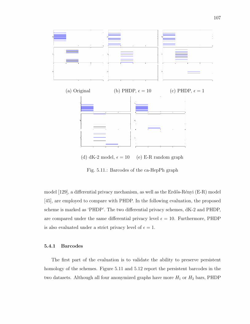
107

(a) Original (b) PHDP, ε = 10 (c) PHDP, ε = 1

(d) dK-2 model, ε = 10 (e) E-R random graph

Fig. 5.11.: Barcodes of the ca-HepPh graph

model [129], a differential privacy mechanism, as well as the Erdos-Renyi (E-R) model

[45], are employed to compare with PHDP. In the following evaluation, the proposed

scheme is marked as ‘PHDP’. The two differential privacy schemes, dK-2 and PHDP,

are compared under the same differential privacy level ε = 10. Furthermore, PHDP

is also evaluated under a strict privacy level of ε = 1.

5.4.1 Barcodes

The first part of the evaluation is to validate the ability to preserve persistent

homology of the schemes. Figure 5.11 and 5.12 report the persistent barcodes in the

two datasets. Although all four anonymized graphs have more H1 or H2 bars, PHDP

108

(a) Original (b) PHDP, ε = 10 (c) PHDP, ε = 1

(d) dK-2 model, ε = 10 (e) E-R random graph

Fig. 5.12.: Barcodes of the Facebook network

has much less distortion in barcodes. In the original ca-HepPh graph, there are 16 H1

bars and 1 H2 bar. PHDP (ε = 10) performs the best in preserving the bars: there

are 22 H1 bars and 1 H2 bar. The PHDP (ε = 1) result has 28 H1 bars and 3 H2

bars. The dK-2 result has 300 H1 bars and 17 H2 bars. The H2 bars are [3, 4) which

implies that the anonymized graph has a 9-sided polygon. The E-R result has 591

H1 bars and 49 H2 bars.

The Facebook barcodes show a similar distribution. In the original graph, there

are 185 H1 bars and 28 H2 bars. And the two numbers are 314 and 71 in the PHDP

(ε = 10) result, 327 and 58 in the PHSP (ε = 1) result, 1142 and 76 in the dK-2

result, and 1688 and 21 in the E-R result.

109

(a) ca-HepPh

(b) Facebook

Fig. 5.13.: Degree distribution

The increase of the H1 and H2 bars suggests that there are more holes in the

anonymized graph. The users ‘on hole’ are farther apart than the users ‘on non-

hole’. While PHDP is confirmed to preserve the persistent homology information

under differential privacy criteria, the utility of dK-2 and E-R anonymized graphs is

questionable because of the injected holes. The evaluation results demonstrate that

110

an OSN with hundreds of nodes or thousands of nodes has very limited number of

holes. Although the building of an OSN seems uncontrolled, the true OSNs are more

strongly connected than artificial graphs in view of persistent homology.

5.4.2 Utility metrics

To demonstrate the links between preserving persistent structures and graph util-

ity, the performance of published graph under utility metrics are compared. The

evaluation includes two graph utility metrics, the degree distribution and the cluster-

ing coefficient, and one application utility metric, the influence maximization.

Degree distribution. Degree distribution is the number of connections of nodes

among the graph. Figure 6.10 shows the degree distribution of the two datasets. The

PHDP and dK-2 anonymized graphs match the degree distribution of the original

graph. Compared to the original ca-HepPh graph, the degree distribution of the

PHDP result (ε = 10) has a root-mean-square error (RMSE) of 0.018, the PHDP

result (ε = 1) has a RMSE of 0.022, the dK-2 result (ε = 10) has a RMSE of 0.018,

but the E-R result has a RMSE of 0.110. Compared to the original Facebook graph,

the PHDP (ε = 10), PHDP (ε = 1), dK-2 and E-R results have RMSE of 0.053, 0.062,

0.036 and 0.072.

The dK-2 anonymized graph maintains a similar degree distribution because it

stores the paired degree information. The PHDP anonymized results suggest that the

persistent homology information may have a soft impact on the degree. Intuitively,

the holes restrict the edges. The E-R model only has the information of the average

degree.

Clustering coefficient. The clustering coefficient shows the level of nodes clus-

tering together. Figure 6.13 is the clustering coefficient of the two datasets. Only

the PHDP anonymized graphs preserve some clustering information. The original

ca-HepPh graph has an average clustering coefficient of 0.52, and it is 0.40 to PHDP

(ε = 10), 0.37 to PHDP (ε = 1), 0.16 to dK-2 (ε = 10) and 0.09 to E-R. The average

111

(a) ca-HepPh

(b) Facebook

Fig. 5.14.: Clustering coefficient distribution

clustering coefficients of the original Facebook graph, the PHDP (ε = 10) result, the

PHDP (ε = 1), the dK-2 result and the E-R result are 0.45, 0.33, 0.30, 0.13 and 0.10,

respectively.

112

As shown in the evaluation of the barcodes, in a increasing order of number

of holes the graphs are the original graph, the PHDP (ε=10), the PHDP (ε=10),

the dK-2 and the E-R results. This order is also the decreasing order of clustering

coefficient. It implies that holes occupy the position of clusters and then decrease the

clustering coefficient. While holes are the opposite of clusters, the PHDP anonymized

graphs preserve the clustering information by protecting the holes. When all holes

in the graph are established, then remaining parts can be filled with clusters. In a

real OSN, this shows that the number of holes are less than the number of clusters.

Hence, storing holes opens a novel angle to maintain the graph structure.

Influence maximization. Influence maximization [73] is an application that first

chooses the important users as seeds, then uses the seeds to influence other people.

In the evaluation, a greedy algorithm based on the independent cascade model [25]

is employed to choose the seeds who have the most ability to broadcast information.

Then the percentage of influenced users are compared among different anonymized

graphs, with the same propagation probability, 0.2.

Figure 5.15 shows the percentage of influenced users. Although all four anonymized

graphs achieve a similar data with the original graph, the PHDP results outperform

the other. Compared to the original ca-HepPh data, the PHDP (ε=10) result has a

RMSE of 0.40, the PHDP (ε=1) has a RMSE of 0.37, the dK-2 result has a RMSE

of 2.50 and the E-R result has a RMSE of 2.30. Compared to the original Facebook

data, the RMSEs are 1.58 of PHDP (ε=10), 2.43 of PHDP (ε=1), 7.57 of dK-2 (ε=10)

and 2.13 of E-R.

This experiment suggests that the PHDP anonymized graphs are good at simulat-

ing the information broadcasting ability of OSNs. Since the influence maximization

problem is closely related to the recommendation and advertisement application, the

PHDP anonymized graph achieves high utility.

Conclusion. This evaluation proves that the PHDP scheme is capable of pre-

serving both persistent homology and differential privacy. The PHDP anonymized

result achieves high utility in both graph metrics and application metrics. Although

113

(a) ca-HepPh

(b) Facebook

Fig. 5.15.: Percentage of influenced users

the PHDP scheme is weaker than the dK-2 scheme in preserving the degree distribu-

tion, it achieves good results under all the utility metrics. It implies that the PHDP

scheme does not target at a specific utility metric but comprehensively preserves the

graph utility.

114

5.5 Conclusion

In this chapter, we address the utility concerns of the published graph by designing

a novel anonymization scheme called PHDP under differential privacy. Unlike the

existing anonymization schemes based on traditional components, e.g., node degree

or clusters, PHDP employs a novel metric called persistent homology. When the

persistent structures are in the form of holes, PHDP preserves the holes as well

as satisfies the differential-privacy criteria. Evaluations on real OSNs confirm that

protecting the holes help PHDP outperform the other schemes in both the graph

utility metric and application metric. In the future, in addition to MCMC as the

approximation method, we will try other methods to optimize the noise injection

phase.

Although persistent homology gives a comprehensive measurement of graph utility,

the proposed anonymization schemes, including PHDP, all passively affect the graph

utility. While we actively set the differential privacy level ε, we cannot direct set the

utility level. In the following chapter, we may discuss how to design an anonymization

scheme which can actively adjust the privacy and utility balance.

115

6. ANONYMIZATION WITH NOVEL METHOD -

SKETCHING

In Chapter 3, 4, and 5, the proposed anonymization schemes based on differential

privacy can only directly adjust the privacy level but not the utility level. In this

chapter, we aim to design a scheme which can actively adjust both utility level and

privacy level, i.e., trim the privacy and utility balance.

In this chapter, we introduce the anonymization scheme based on All-Distance

Sketch (ADS). Sketching can significantly limit attackers’ confidence, as well as pro-

vide accurate estimation about shortest path length and other utility metrics. Be-

cause sketching removes large amounts of edges, it is invulnerable to seed-based and

subgraph-based de-anonymization attacks. However, existing sketching algorithms

do not add dummy edges and paths. Adversaries have low false positive in extracting

linking information, which challenges the privacy performance. We propose the novel

bottom-(l, k) sketch to defend against these advanced attacks. We develop a scheme

to add and delete enough edges to satisfy our privacy demand.


1. We embed the ADS algorithm, which preserves the distance information with

bounded error, in OSN anonymization.

2. We propose the bottom-(l, k) sketch algorithm to improve the privacy of our

anonymization scheme, which is suitable to defend against the advanced attacks.

3. We design the edge addition/deletion algorithm based on the ADS graph. Our

algorithm intelligently add/delete edges without interrupting the properties of

bottom-(l, k) sketch.

This chapter is previously published as a conference paper in IEEE International

Conference on Sensing, Communication, and Networking (SECON), 2019 [53].

116

6.1 Preliminary

In this chapter, an OSN is modeled as an unweighted graph G = (V,E), where V

is the set of all vertices and E is the set of all edges. |V | shows the cardinality of set

V , i.e., the number of vertices. Moreover, we denote the ADS graph as Gs = (V,Es)

and the final published graph as Gp = (V,Ep).

MinHash sketch. MinHash sketch randomly summarizes a subset of k items

from the original set [16]. Researchers designed three variations of MinHash sketch,

named bottom-k, k-mins, and k-partition [30, 32, 34]. Specifically, bottom-k sketch

samples k items with the lowest hash values; k-mins sketch samples one item each

iteration with the lowest hash value and repeats the iteration k times (in each iter-

ation, the hash values are different); k-partition sketch divides the original set into

k subsets and samples one item from each subset. When the hash value of each

item is randomly assigned, the sampled subset is a sketch of the original set. Among

these sketching methods, bottom-k was proved to have the following benefits: (1)

uniformly distributed ranking is an unbiased estimator; (2) with the same value of k,

it gives higher performance in distance estimation than k-mins. Hence, our chapter

concentrates on bottom-k sketch.

All-distance sketch. Based on MinHash sketch, researchers define the all-

distance sketch to sample the data with graph structures [31]. The main idea of

ADS is to keep nodes with the lowest hash values within a specific distance to the

central node. In particular, we uniformly assign a rank r(u) to each node u, where

r(u) ∈ [0, 1]. ADS(v) contains a set of nodes and their distances to the central node

v. If u ∈ ADS(v), comparing all nodes w with distances dvw 6 dvu, node u has the

bottom-k ranks.

Figure 6.1 gives an example of ADS when k = 1. In this graph, each node has

a number to show the rank, e.g., r(A) = 0.74. Each edge has a number to show

the distance, e.g., dAB = 1. When sketching ADS(A), we first add node A itself in

its ADS. Then, we examine nodes within distance one, i.e., node B. Node B has the

117

A

B

C

D

1

2

3

0.74

0.37

0.62

0.23

Fig. 6.1.: Example of bottom-1 ADS. ADS(A) = {(A, 0), (B, 1), (D, 3)}.

bottom-1 rank so add it to ADS(A). We examine nodes within distance two, i.e.,

nodes {B,C}. Because node C does not have the bottom-1 rank in the set, we do not

add it to ADS(A). Finally, in the set of nodes within distance three, node D has the

bottom-1 rank. Hence, ADS(A) = {(A, 0), (B, 1), (D, 3)}.

Hitherto two main approaches are introduced to compute ADS [31]. One combines

pruning algorithms with Dijkstra’s algorithm. The other is based on the dynamic

programming process of the Bellman-Ford algorithm. Because the ADS computa-

tion algorithms can ignore nodes with high ranks, calculating ADS for one node is

more efficient than other traversing algorithms, e.g., breadth-first search. Cohen and

Kaplan prove that the bottom-k ADS is O(k|E| log |V |) [32].

6.2 Threat modeling

In this section, we model the ability of adversaries to capture true relationships,

i.e., to ascertain the existence of edges in the original graph G, from examining

the published graph Gp. Modeling helps us derive privacy and utility of our ADS

anonymization scheme. Specifically, we model two kinds of adversaries who both

have some information about the total number of added/deleted edges and the ADS

anonymization scheme. The first kind of adversary focuses on target relationships.

118

The other kind of adversary wants to collect as much information as they can. These

two kinds of adversaries are called ‘spear attacker’ and ‘general attacker’, respectively,

in the following sections.

6.2.1 Spear attacker

In a spear attack, an attacker has some target users and he or she wants to know

the properties of these users, e.g., the distances between two target users. The OSN

service provider cannot predict the target users; however, the service provider can

calculate the average of privacy and utility among all users to simulate an attack.

We use a parameter C to show the average confidence of the adversary to believe

an edge exists in the original graph G when the adversary has the ADS graph Gs. In

our assumption, this adversary knows the original graph size and the parameter of k

in the ADS graph. In a graph with |V | nodes, there are at most |Ef | edges, where

|Ef | = |V |2−|V |2

. Then the average confidence C is given by,

C =|Es||Ef |

+|Ef | − |Es||Ef |

· |Ef | − |E||Ef | − |Es|

=|Ef |+ |Es| − |E|

|Ef |. (6.1)

Here |Es||Ef |is the probability that the adversary chooses a pair of nodes that has an

edge in Gs. Because all edges in Gs are inherited from edges in G, they are all true

relationships.|Ef |−|Es||Ef |

is the probability that the adversary chooses a pair of nodes

that does not have an edge in Gs. For these nonexistent edges, the probability that

the edge also does not exist in G is|Ef |−|E||Ef |−|Es|

. Hence, the adversary has the confidence

C =|Ef |+|Es|−|E|

|Ef |.

Utility of the ADS graph can be evaluated in several ways, according to specific

utility metrics. For example, the theoretical bounds of distance is given by,

duv ∈[duv,

(2

⌈log|V |logk

⌉− 1

)duv

], (6.2)

where duv is the true distance in G and duv is the distance in the sketched graph

Gs [33].

119

A C

F

B

G

D E

A C

F

B

G

D E

A C

F

B

G

D E

A C

F

B

G

D E(a) Original graph

A C

F

B

G

D E

A C

F

B

G

D E

A C

F

B

G

D E

A C

F

B

G

D E(b) ADS graph

A C

F

B

G

D E

A C

F

B

G

D E

A C

F

B

G

D E

A C

F

B

G

D E

(c) ADS graph with edge pertur-

bation

A C

F

B

G

D E

A C

F

B

G

D E

A C

F

B

G

D E

A C

F

B

G

D E

(d) Second-round ADS graph

Fig. 6.2.: Example of second-round ADS attack

6.2.2 General attacker

A general attacker does not have target users. Instead, he or she would like to

infer as much information as possible from the published graph. For instance, the

attacker wants to know if two users are connected in the original graph when these

two users are connected in the published graph. Because important edges have a

higher probability of being preserved in the ADS graph, the adversary can apply a

second-round ADS attack to eliminate some unimportant edges.

120

Figure 6.2 shows an example of that attack. In Figure 6.2(c), we use an anonymiza-

tion algorithm to add perturbed edges. However, having this perturbed graph, the

adversary can make the ADS graph from Figure 6.2(c), which is shown in Figure

6.2(d).

Edges in the second-round ADS graph have a high probability of being the edges

in the original graph. For example, path A− B− C is the only path that maintains

the distance between A and C. The anonymization algorithm cannot use other paths

to replace this path, because if it did, the distance measure between A and C would

not be true.

By contrast, the misleading edges, e.g., edge E−C, are eliminated in the second-

round ADS graph. If the anonymization algorithm cannot add dummy edges that

have the same importance as the edges in the ADS, other dummy edges will not

obfuscate adversaries as intended. After applying a second-round ADS to eliminate

misleading edges, true edges in the original graph become distinct.

6.3 Scheme

When analyzing two kinds of adversaries, we find two main problems with directly

applying ADS to anonymize OSNs. First, ADS only has edge removal, so spear

attackers have no false positives when extracting linking information. Second, a

second-round ADS attack enables the general attackers to extract linking information

even though we randomly add dummy edges to the graph. Hence, we need to design

an anonymization algorithm to effectively sketch the graph and add dummy edges.

In order to defend against the second-round ADS attack, we propose the bottom-

(l, k) ADS graph, which has the following definition:

Definition 5 (Bottom-(l, k) ADS graph). If node u ∈ ADS(v) with the bottom-

k sketch, there should be at least l paths between u and v in Gs, except that duv = 1.

The graph Gs is the bottom-(l, k) ADS graph of G if and only if for all nodes v in G,

Gs contains all nodes in v’s ADS and all these l paths.

121

Note that it is meaningless to build l paths between two connected nodes. Because

OSNs are simple graphs without multiple edges, the sketched graph should also be

simple graphs, otherwise the adversary can easily remove redundant edges.

The purpose of our scheme is to output a published graph Gp when the input is

the original graph G. Gp is based on the bottom-(l, k) ADS graph Gs and Gp should

maintain a balance between utility and privacy. Our scheme has the following parts:

1. We design an algorithm to generate the bottom-(l, k) ADS graph Gs.

2. We analyze the privacy and utility impact of edge addition and deletion, which

guides graph perturbation.

3. We change the edges in Gs and publish Gp to achieve the privacy and utility

balance.

6.3.1 Bottom-(l, k) ADS

Existing bottom-k ADS algorithms have proven to be effective and efficient. How-

ever, these algorithms focus on generating the ADS sets and graphs, while our purpose

is to preserve privacy in the sketched graph. For privacy purpose, reviewing the pre-

vious example in Figure 6.1, after knowing node D is in ADS(A), we should build at

least l paths between nodes A and D.

The approach to draw the sketched graph has two parts: (A) extracting ADS

for each node, and (B) building paths between nodes. Our new sketching algorithm,

Algorithm 9, has the following steps:

1. We get the distance matrix Md from the graph.

2. For each node in the matrix, we get its ADS set, and mark the nodes in this

set.

3. We build a residual matrix Mr that initially sets the marked place to l.

4. For each number l in the residual matrix, we try to build l paths in three ways:

directly linking, leaving to other paths, and adding new edges.

122

Algorithm 9 Bottom-(l, k) ADS

Input: Original graph G

Output: Sketched graph Gs, newly added edge |Ea|

1: Get distance matrix Md of the graph G

2: For each node u, if node v ∈ ADS(u), mark position (v, u)

3: Create residual matrix Mr. If position (v, u) is marked in Md, set Mr(v, u) = l.

4: Create graph Gs with no edge.

5: for each position (v, u) in Mr do

6: If Md(v, u) = 1, link u and v, set Mr(v, u) = 0.

7: Else if there is a node w ∈ ADS(v), and it has Md(v, u) = Md(v, w)+Md(w, u)

and Md(v, u) > 2, set Mr(v, u) = 0.

8: Else add Mr(v, u) paths between v and u

9: end for

A B C

D E F

G H I

(a) Original graph

A B C

D E F

G H I

2

3

2

(b) ADS graph

Fig. 6.3.: Graph example of ADS

Here we use an example to show the sketching steps. Initially, we have the original

graph G, which is shown in Figure 6.3(a). Our purpose is to generate the bottom-

(2, 1) sketched graph. This means that the ADS set is the bottom-1 sketch of the

graph. And for each node u ∈ ADS(v), there are at least 2 paths between u and v.

123

In the first step, we build the distance matrix Md, Md(u, v) = duv. In the second

step, we extract the ADS set for each node. For example, if we want to get the ADS

set of nodes I and F, we extract the two lines related to these two nodes (shown in

Figure 6.4).

node A B C D E F G H Irank 0.6 0.1 0.3 0.2 0.8 0.4 1 0.5 0.9

I 0.9 4 3 2 3 2 1 2 1 0F 0.4 3 2 1 2 1 0 3 2 1

Fig. 6.4.: A part of Md with nodes I and F

Having a line of Md, we can get the ADS set for the corresponding nodes. For

example, we have ADS(I) = {B,C,F, I} and their corresponding distances. In Figure

6.4, we mark these nodes in blue. In Figure 6.3(b), we link the nodes in ADS(I) with

node I. The dotted edge between C and I, for instance, means that C ∈ ADS(I) and

the distance between the two nodes is 2.

In the third step, we build the residual matrix Mr to show the number of residual

paths between nodes. Initially, Mr is a zero matrix. If a position is marked in blue

in Md, we set this position to l. There is an exception for the same node cases, e.g.,

Mr(I, I) = 0.

124

node A B C D E F G H Irank 0.6 0.1 0.3 0.2 0.8 0.4 1 0.5 0.9

I 0 0 2 2 0 0 2 0 0 0F 0 0 2 2 0 0 0 0 0 0

Fig. 6.5.: Initial Mr with nodes I and F

In the forth step, we need to build paths according to Mr. Specifically, there are

three cases: First, if we need to build l paths between u and v, and the two nodes

are directly linked in G, we link the two nodes in Gs to complete this step. The edge

F−I in Figure 6.3(b) is an example of this case.

Second, we try to find an intermediate node w ∈ ADS(v) between u and v. It is

clear that if there are l paths between w and u (or between w and v), there should be

at least l paths between u and v. However, we cannot leave all building tasks to w

without checking the distances. Because between two directly connected nodes there

is only the direct link, then if both u− w and v − w are directly connected, there is

only one path between u and v instead of l different paths. Hence, we require that

Md(u, v) > 2, which means that the intermediate node is disconnected with at least

one end node. Path B−I is an example of the second case. However, path C−I is a

counter example since Md(C, I) = 2.

Third, we need to build paths according to the updated Mr. In this example,

we only need to build 2 paths between B−F and 2 paths between C−I. The process

of building paths is the same as the process of choosing intermediate node sets.

Consequently, building l paths is the same as choosing l node sets, and every two sets

differ by at least one element. We have two cases in choosing intermediate nodes:

(1) The intermediate nodes can link the two end points with the desirable dis-

tance. For example, node E is the intermediate node between path B−F. The chosen

intermediate nodes should satisfy the following criteria: First, the distances between

125

two end points should be larger than the distance between each intermediate nodes

and each one of end points. Second, the distances between the intermediate nodes

and one end point are in an incremental order, e.g., 1, 2, 3,... In this example,

Md(B,E) = 1 and Md(B,F) = 2. Although E /∈ ADS(B) and E /∈ ADS(F), choosing

E as the intermediate node between B and F still maintains the distance. Similarly,

path C−F−I and path B−C−F are in this case.

(2) When we cannot find intermediate nodes in the first case, we choose a node set

{w} with the lowest distance increment. For example, we need to build another path

between C and I in addition to C−F−I. When we choose node E (or B, H) as the

intermediate node, we have the lowest distance increment 2. In general cases, when

{w} = {w1, w2, ..., wn}, and the two end nodes are marked as u and v, it requires that

Md(u,w1) +Md(w1, w2) + ...+Md(wn, v)−Md(u, v) is lowest compared to other sets

of intermediate nodes.

The first case do not change the distances between nodes because they still sample

edges in the original graph to build paths. However, the second case builds new edges

and changes distances between some pairs of nodes. For example, after adding path

C−E−I, dCE changes. Fortunately, our algorithm has tolerance of edge addition, and

its impact is analyzed in Section 6.3.2. Here we need to record the number of added

edges, denoted by |Ea|. In the following sections, these edges occupies a part of our

edge changing budget.

Finally, we get the sketched graph Gs. Gs of this example is shown in Figure 6.6.

6.3.2 Impact analysis of edge addition/deletion

As discussed in Section 6.2.1, a simple ADS graph is not suitable for preserving

privacy in OSN data publication. In this section, we analyze the achieved privacy

and preserved utility when we add/delete edges in the ADS graph.

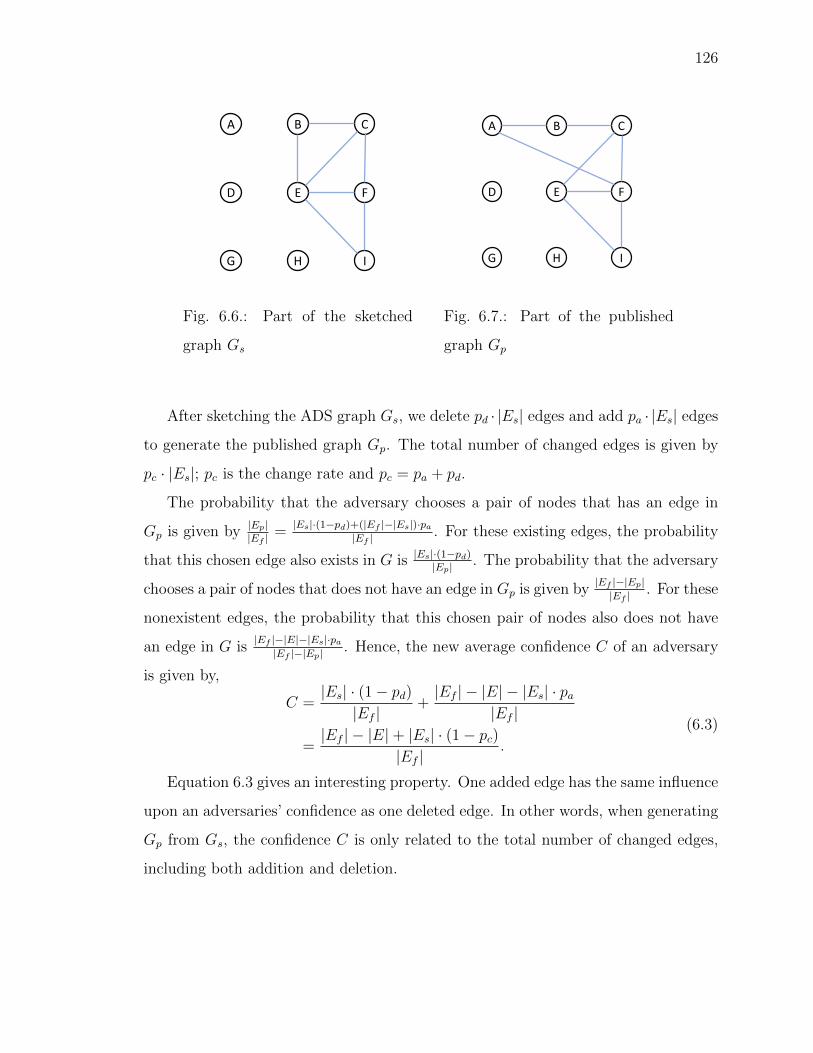
126

A B C

D E F

G H I

Fig. 6.6.: Part of the sketched

graph Gs

A B C

D E F

G H I

Fig. 6.7.: Part of the published

graph Gp

After sketching the ADS graph Gs, we delete pd · |Es| edges and add pa · |Es| edges

to generate the published graph Gp. The total number of changed edges is given by

pc · |Es|; pc is the change rate and pc = pa + pd.

The probability that the adversary chooses a pair of nodes that has an edge in

Gp is given by |Ep||Ef |

=|Es|·(1−pd)+(|Ef |−|Es|)·pa

|Ef |. For these existing edges, the probability

that this chosen edge also exists in G is |Es|·(1−pd)|Ep| . The probability that the adversary

chooses a pair of nodes that does not have an edge in Gp is given by|Ef |−|Ep||Ef |

. For these

nonexistent edges, the probability that this chosen pair of nodes also does not have

an edge in G is|Ef |−|E|−|Es|·pa|Ef |−|Ep|

. Hence, the new average confidence C of an adversary

is given by,

C =|Es| · (1− pd)

|Ef |+|Ef | − |E| − |Es| · pa

|Ef |

=|Ef | − |E|+ |Es| · (1− pc)

|Ef |.

(6.3)

Equation 6.3 gives an interesting property. One added edge has the same influence

upon an adversaries’ confidence as one deleted edge. In other words, when generating

Gp from Gs, the confidence C is only related to the total number of changed edges,

including both addition and deletion.

127

A

B C

D

E F

G H

Fig. 6.8.: Example of edge addition and deletion; solid edges mean true relationships

in Gs

How does the edge addition/deletion affect utility? We analyze the example in

Figure 6.8. We assume node D is in ADS(A). In this example, we would like to

switch the path from A−B−C−D to A− E− F−D. This means that we need to

delete three edges and add the new edge E−F. In this example, dAD = 3 is the total

length of the path. In a general case, if we add d′ edges (d′ 6 d), the total number

of changed edges is given by d + d′. Moreover, the total number of changed edges is

also given by pc · |Es|, we have pc · |Es| = d+ d′.

When calculating utility metrics, e.g., distances between nodes, we find that newly

added edges cause some wrong results. These wrong results happen only if the follow-

ing two conditions are satisfied: (1) We call the end nodes of newly added edges as

‘trigger node’. Then the source node should be a ‘trigger node’, i.e., nodes E and F.

When the source node is not a ‘trigger node’, e.g., nodes G and H, the utility metrics

calculation is correct. (2) The distance between the source node and the target node

should be farther than the distance between another ‘trigger node’ and the target

node. For example, when calculating dDE, the shortest path uses the newly added

edge E− F and the distance is incorrect. In another example, when calculating dDF,

the newly added edge is not used. In a general case, each ‘trigger node’ chooses a

target node and outputs a wrong distance result with probability about 50%. If ‘trig-

128

ger nodes’ exists, each node averagely has 50% probability to give a wrong distance

result. The number of ‘trigger nodes’ is d′ + 1. Hence, the probability of getting a

correct distance is given by,

Pdistance = 1− d′ + 1

2|V |

= 1− pc · |Es| − d+ 1

2|V |

6 1− pc · |Es|+ 2

4|V |.

(6.4)

Reviewing the impact of edge addition/deletion upon privacy and utility, we

made the following observation: When the release graph can give confidence C =

|Ef |−|E|+|Es|·(1−pc)|Ef |

, the probability of getting the distance between nodes u and v as

described in Equation 6.2 is given by Pdistance 6 1− pc·|Es|+24|V | . Therefore, both privacy

and utility is affected by pc, i.e., the total number of added and deleted edges.

6.3.3 Edge changing

Based on the impact analysis, this subsection provides method to further perturb

the sketched graph Gs. We control the privacy and utility tradeoff in the edge chang-

ing step by setting a desirable edge change rate pc. Having a target pc, we would like

to change pc · |Es| edges in total, and publish the graph Gp. Since |Ea| edges have

already been added when sketching Gs, we need to change |Ec| edges. |Ec| is the edge

changing budget and |Ec| = pc · |Es| − |Ea|.

The main challenge of this part is that our perturbation should not violate the

properties of bottom-(l, k) sketch. Specifically, if the perturbation deletes one path

between u and v in this phase, we should add another path from u to v. Otherwise, our

published graph cannot preserve as much utility as discussed in the impact analysis.

Hence, our edge changing algorithm, Algorithm 10, has the following steps:

1. We build an edge-to-path matrix Mp to show the mapping relationships from

edges to paths.

129

Algorithm 10 Edge changing

Input: Sketched graph Gs, change rate pc, number of added edges |Ea|

Output: Final published graph Gp

1: Get number of edges need to change |Ec| = pc · |Es| − |Ea|

2: Get path-to-edge matrix Mp

3: Initialize Gp as Gs

4: while |Ec| > 0 do

5: Randomly pick an edge in Gp, delete it, |Ec|− = 1

6: Search this edge’s mapping paths.

7: For each path, find the alternative path and build it.

8: For each adding edge, |Ec|− = 1.

9: Update Mp

10: end while

2. We randomly choose an edge in Mp, delete that edge and add other edges to

maintain the paths.

3. We continue doing the second step until our budget |Ec| is exhausted.

Similarly, we explain the details of edge changing steps in this example. The input

graph is Gs, shown in Figure 6.6. Our purpose is to generate the published graph Gp.

path edge B-C B-E B-F C-E C-F E-F E-I F-I E-H F-H H-IF-I 0 0 0 0 0 0 0 1 0 0 0C-F 0 0 0 0 1 0 0 0 0 0 0C-I 0 0 0 1 1 0 1 1 0 0 0B-F 1 1 0 0 1 1 0 0 0 0 0B-I 1 1 0 0 1 1 0 1 0 0 0

Fig. 6.9.: Edge-to-path matrix Mp of the graph in Figure 6.6

130

In the first step, we build the edge-to-path matrix Mp, which is shown in Figure

6.9. The first line shows the edges in Gs. An edge is marked in grey while it exists

in the original graph G. In the following steps, we choose only these marked edges to

delete because deleting other edges does not influence the confidence of the adversary.

The first column shows the paths (named in two end points). The remaining part

contains 0s and 1s to show whether an edge contributes to paths between the two

end nodes.

In the second step, we randomly choose an edge and delete it. After we delete

an edge, we search Mp for the corresponding paths and build these paths. In the

path-building process, we search for intermediate nodes, which have the same two

cases as previously discussed in Section 6.3.1.

In this example, we plan to delete the edge B−E. From matrix Mp, we find that we

need to build one new path for B−F and one for B−I, when deleting B−E. Because

path B−F is part of path B−I, building a new path with B−F will also bring a new

path with B−I. Hence, we only focus on building B−F here. dBF = 2 means we need

to find one intermediate node. Because we cannot find the intermediate node in the

first case, i.e., with the desirable distance, we need to search nodes in the second case,

i.e., with the lowest distance increment. In this example, it is node A. Then, we link

edges B−A and A−F to form the path B−F.

In the third step, we count the number of edges that have already been added or

deleted and compare this number with our budget |Ec|. In this example, we delete

one edge B−E and add two edges B−A and A−F, so the budget is consumed by

three. If |Ec| 6 3, the budget is exhausted and we meet our privacy requirement.

Finally, we get the published graph Gp. Gp of our example is shown in Figure 6.7.

131

Table 6.1.: Number of edges and non-edges in G and Gp

Edges in G Non-edges in G Sum

Edges in Gp |Es| · (1− pd) |Es| · pa |Es| · (1− pd + pa)

Non-edges in Gp |E| − |Es|+ |Es| · pd |Ef | − |E| − |Es| · pa |Ef | − |Es| · (1− pd + pa)

Sum |E| |Ef | − |E| |Ef |

6.4 Analysis

6.4.1 Privacy analysis

Privacy is always measured from the third parties’ perspective, i.e., how much

information is released to the third parties. This chapter focuses on edge privacy.

Hence, C denotes the confidence of the attacker about a target edge exists (or does

not exist) in the original graph G, when he or she holds the published graph Gp.

C =|Ef | − |E|+ |Es| · (1− pc)

|Ef |

=|V |2 − |V | − 2|E|+ 2|Es| · (1− pc)

|V |2 − |V |.

(6.5)

Differential privacy gives another measurement of privacy. It formalizes the re-

lationship between G and Gp. Specifically, for an anonymization mechanism A to

achieve ε-differential privacy, two neighboring graphs G1 and G2 should have the

following relationship,

Pr[A(G1) ∈ S] ≤ eε × Pr[A(G2) ∈ S], (6.6)

where S is the output space of A. To satisfy edge differential privacy, the neigh-

boring graphs G1 and G2 have one edge difference. Equation 6.6 suggests that the

probability of Gp having one specific edge is not greater than eε times of the proba-

bility of this edge does not exist, and vice versa. Hence, information leakage in Gp is

bounded with the parameter ε.

Here, we propose a similar privacy bound in an average manner.

132

Property 4. To an attacker who holds the published graph Gp, the average proba-

bility that all edges exist (resp. do not exist) in the original graph is not higher than eεa

times the probability that these edges do not exist (resp. exist) in the original graph,

where εa = ln(|Es|·(|Ef |−|E|)·(1−pd)·(1−pd+pa)

|Ef |·|E|·pa+|Ef |−|Es|·(1−pd+pa)

|Ef |· (|E|−|Es|+|Es|·pd)(|Ef |−|E|)

(|Ef |−|E|−|Es|·pa)·|E|

).

Proof: Without loss of generality, we assume the attacker randomly chooses a pair

of nodes (u, v). In the two neighboring graphs G1 and G2, this node pair is an edge

in G1 and a non-edge in G2. Hence, we have (u, v) ∈ E1 and (u, v) /∈ E2. After

anonymization, the two published graphs Gp1 and Gp2 should have the same output.

There are two different cases, (u, v) ∈ Ep and (u, v) /∈ Ep.

In the first case, the two published graphs both contain edge (u, v), S = {(u, v) ∈

Ep}. We have,

Pr[A(G1) ∈ S] = Pr[(u, v) ∈ Ep1|(u, v) ∈ E1]

Pr[A(G2) ∈ S] = Pr[(u, v) ∈ Ep2|(u, v) /∈ E2](6.7)

Table 6.1 shows the number of edges in G and Gp. For example, the number of

node pairs that are connected both in G and Gp is |Es| · (1−pd). Table 6.1 gives that,

Pr[(u, v) ∈ Ep1|(u, v) ∈ E1] =Pr[(u, v) ∈ Ep1 ∩ (u, v) ∈ E1]

Pr[(u, v) ∈ E1]

=|Es| · (1− pd)

|E|

Pr[(u, v) ∈ Ep2|(u, v) /∈ E2] =Pr[(u, v) ∈ Ep2 ∩ (u, v) /∈ E2]

Pr[(u, v) /∈ E2]

=|Es| · pa|Ef | − |E|

(6.8)

Then,

eε1 =Pr[A(G1) ∈ S]

Pr[A(G2)]=

(|Ef | − |E|) · (1− pd)|E| · pa

(6.9)

133

In the second case, the two published graphs both contain non-edge (u, v), S =

{(u, v) /∈ Ep}. Similarly, we get,

Pr[A(G1) ∈ S] = Pr[(u, v) /∈ Ep1|(u, v) ∈ E1]

=|E| − |Es|+ |Es| · pd

|E|

Pr[A(G2) ∈ S] = Pr[(u, v) /∈ Ep2|(u, v) /∈ E2]

=|Ef | − |E| − |Es| · pa

|Ef | − |E|

eε2 =(|E| − |Es|+ |Es| · pd)(|Ef | − |E|)

(|Ef | − |E| − |Es| · pa) · |E|

(6.10)

The probabilities of the first and second case are |Es|·(1−pd+pa)|Ef |

and|Ef |−|Es|·(1−pd+pa)

|Ef |,

respectively. Finally, we can get the average privacy parameter εa.

eεa =|Es| · (1− pd + pa)

|Ef |eε1

+|Ef | − |Es| · (1− pd + pa)

|Ef |eε2

εa = ln

(|Es| · (|Ef | − |E|) · (1− pd) · (1− pd + pa)

|Ef | · |E| · pa

+|Ef | − |Es| · (1− pd + pa)

|Ef |

∗ (|E| − |Es|+ |Es| · pd)(|Ef | − |E|)(|Ef | − |E| − |Es| · pa) · |E|

)(6.11)

The main idea behind Property 4 is to apply the parameter eεa to measure the

information leakage. Our sketch scheme does not follows steps in the traditional

differential privacy mechanisms, e.g., using sensitivity to calibrate the amount of

noise and designing the perturbed distribution. However, we claim that sketching

has a similar impact to data with traditional differential privacy perturbation with

the proof.

134

Fig. 6.10.: Degree distribution, Facebook.

Fig. 6.11.: Shortest path length distribution, Face-

book.

6.5 Evaluation

In this section, we evaluate our sketching scheme over three real-world datasets,

namely ca-HepTh, Facebook, and Enron [88]. We demonstrate the utility of our

published graphs with different (l, k) and desired change rate pc. For comparison

135

Fig. 6.12.: Shortest path length distribution, ca-

HepPh.

Fig. 6.13.: Clustering coefficient distribution, ca-

HepPh.

purposes, we implement one anonymization mechanism as reference, which is the

differential privacy algorithm with the dK-2 model [129, 148]. We use Equation

6.11 to calculate the corresponding εa of our scheme; then we set ε = εa as the

136

Fig. 6.14.: Betweenness distribution, Facebook

Fig. 6.15.: Closeness centrality distribution, Enron

privacy requirement in the reference dK-2 anonymization method. When the two

anonymization schemes have similar privacy requirement, we evaluate and compare

the utility preservation of the published graphs.

137

Degree. The degree of a node in the network is the number of edges incident

to the node. While the dK-2 model preserves the degree of nodes, our sketching

algorithm removes large amounts of unnecessary edges, which has a great impact on

degree. Figure 6.10 shows the degree distribution of the Facebook dataset. When

(l, k, pc) = (1, 2, 0.2), we have εa = 0.92. When (l, k, pc) = (2, 2, 0.2), we have εa =

1.01. Then the degree distributions of corresponding εs are also analyzed.

The average degrees of the original Facebook graph, our sketching result (l = 1),

the dK-2 anonymized result (ε = 0.92), our sketching result (l = 2), and the dK-2

anonymized result (ε = 1.01) are 36.14, 6.51, 40.08, 7.36, and 41.74, respectively. In

all of our experiments, there are about 20% edges remaining in our sketched results.

The deletion of edges greatly impacts the degree distribution of our published graph.

Moreover, when there are less paths remaining in the graph (lower l), more edges are

deleted.

Average shortest path length. Average shortest path length implies the in-

formation transmission speed in the network. The dK-2 node can only indirectly

preserve the shortest path length information when combining two edges with one

same-degree node. ADS is appropriate to preserve distance information, as is our

anonymized sketching algorithm. Figure 6.11 and 6.12 show the shortest path length

distribution in the Facebook and the ca-HepPh datasets. In the ca-HepPh dataset,

when (l, k, pc) = (2, 2, 0.3), we have εa = 1.20. When (l, k, pc) = (2, 2, 0.2), we have

εa = 1.43. Then the shortest path length distributions of corresponding εs are also

analyzed.

The average shortest path length of the original ca-HepPh graph, our sketching

result (pc = 0.3), the dK-2 anonymized result (ε = 1.20), our sketching result (pc =

0.2), and the dK-2 anonymized result (ε = 1.43) are 2.78, 3.36, 6.14, 3.04, 6.11,

respectively. While the dK-2 anonymized graphs double the shortest path lengths,

our published graphs preserve these lengths with only about 20% edges. Moreover,

when there are more paths (higher l) or lower privacy demand (lower pc), our sketched

graph can more precisely preserve the shortest path length information.

138

Clustering coefficient. Clustering coefficient is a measure of how nodes in a

graph tend to cluster together. Figure 6.13 shows the clustering coefficient distribu-

tion of the ca-HepPh dataset. The average clustering coefficient of the original ca-

HepPh graph, our sketching result (pc = 0.3), the dK-2 anonymized result (ε = 1.20),

our sketching result (pc = 0.2), and the dK-2 anonymized result (ε = 1.43) are 0.27,

0.10, 0.05, 0.18, 0.02, respectively. Neither anonymization algorithm can preserve this

information theoretically or experimentally.

Betweenness. Betweenness centrality shows the number of shortest paths that

pass through a node. Figure 6.14 shows the betweenness distribution of the Facebook

dataset. The average betweenness of the original Facebook graph, our sketching result

(l = 1), the dK-2 anonymized result (ε = 0.92), our sketching result (l = 2), and the

dK-2 anonymized result (ε = 1.01) are 0.0026, 0.0035, 0.0002, 0.0034, and 0.0002,

respectively.

Because our anonymized sketching algorithm preserves a part of shortest paths,

its distribution is very similar to the original distribution. Moreover, in our bottom-

(l, k) sketch, when we slightly increase l, the published graph has better performance

in preserving betweenness than the basic bottom-k sketch. Because there always

have more than one path between two nodes, l is a compensation to edge removal in

sketching.

Closeness centrality. Closeness centrality measures the reciprocal of the sum of

the length of the shortest paths between the node and all other nodes in the graph.

Figure 6.15 shows the closeness centrality distribution of Enron network. In the Enron

dataset, when (l, k, pc) = (2, 1, 0.2), we have εa = 1.00. When (l, k, pc) = (2, 2, 0.2),

we have εa = 1.11. Then the closeness centrality distributions of corresponding εs are

also analyzed.

The average closeness centrality of the original Enron graph, our sketching result

(k = 1), the dK-2 anonymized result (ε = 1.00), our sketching result (k = 2), and the

dK-2 anonymized result (ε = 1.11) are 0.34, 0.30, 0.17, 0.30, and 0.18, respectively.

Similarly, we find that our anonymized sketching algorithm preserves closeness cen-

139

trality distribution better than the dK-2 anonymization algorithm. To conclude, the

proposed scheme outperforms the existing dK-2 scheme in preserving utility under

the similar privacy requirement, which shows a better balance between privacy and

utility in the published graph.

6.6 Conclusion

In this chapter, we apply sketching to anonymize OSN data. We propose the

bottom-(l, k) sketch algorithm to prevent second-round ADS attack. We introduce

the edge changing algorithm to increase attackers’ uncertainty and strike the balance

between utility and privacy. The experiments show that our anonymized sketching

algorithm can better preserve graph utility when the privacy preservation level is close

to differential privacy.

In this chapter and previous chapters, we study the anonymization scheme, e.g.,

the privacy and utility preservation, from the defenders’ point of view. However, the

attacker also plays an important role in the privacy preservation problem. Analyzing

the attackers’ abilities and behaviors may give us hints about how to prevent them.

In the following chapters, we may discuss how can the attackers de-anonymize the

anonymized data.

140

7. DE-ANONYMIZATION WITH MAPPING SEEDS -

PERSISTENT STRUCTURES

In previous four chapters, we study the OSN data anonymization problem. In this

chapter, we focus on the OSN data de-anonymization problem. We start with a tradi-

tional de-anonymization techniques called seed-and-grow mapping. The OSN service

providers may sequentially release data and the adversaries can get the dynamic OSN

data. This chapter introduces a scheme which extracts dynamic information and im-

proves existing seed finding algorithm.

In this chapter, we deploy persistent homology to capture the evolution of OSNs.

Persistent homology barcodes show the birth time and death time of holes, i.e., poly-

gons, in dynamic OSNs. By extracting the evolution of holes, persistent homology

captures the addition/deletion of edges, which is the crucial feature of dynamic OSNs.

After extracting the evolution of holes, we apply a two-phase de-anonymization at-

tack. First, holes are mapped together according to the similarity of birth/death

time. Second, already mapped holes are converted into super nodes, which are seed

nodes; we then grow the mapping based on these seed nodes. Our de-anonymization

scheme is extremely compatible to the adversaries who suffer latency in relationship

collection, which is very similar to real-world cases.


1. We probabilistically model the ability of adversaries to get the true relationships,

which is realistic in real-world cases.

2. We apply persistent homology to capture the persistent structures in dynamic

graphs.

3. We introduce a seed-and-grow algorithm to map nodes in dynamic graphs.

This chapter is previously published as a conference paper in IEEE International

Conference on Communications (ICC), 2019 [51].

141

7.1 Threat model

In this chapter, the OSN service provider continues releasing the time-series graph

GA. GA = (V A, EA), where V A is the set of vertices, if that vertex exists in at least

one time period in GA, and EA is the set of edges. GA is modeled as a set of static

graphs. GA = {GA1 , G

A2 , ..., G

An}, where GA

i is the graph in i-th epoch. Meanwhile,

the attacker builds another time-series graph GB with his/her background knowledge.

The purpose of this chapter is to map nodes from GB to nodes in GA.

In this chapter, we assume all nodes in GB form a node set V B, which is the subset

of V A (all nodes in GA). The edge set EAs is a subset of the edge set EA, EA

s contains

all edges whose both nodes have corresponding nodes in V B. When discussing the

edges in GA, we only focus on the edges in EAs .

However, the mapping task has two major challenges. First, the service provider

does not directly release the graph. The service provider not only removes the identi-

ties in each static graph, but also perturb the graph before releasing. In the original

graph, because new links may form and old links may drop, the self mapping of GA

is as hard as the de-anonymization work between two static graphs.

Second, the attacker cannot have perfect background knowledge graph, which is

reflected in GB. In this chapter, we model the shortfall of the attacker’s background

knowledge by two factors: latency and unknown. Latency means that for some rela-

tionships forming/dropping in epoch i in the original OSN, the attacker knows this

relationship is forming/dropping in epoch j, where j > i. Unknown means the at-

tacker always have wrong information about some specific relationships. Particularly,

if an edge is added/deleted in GAi , GB

j adds/deletes that corresponding edge with

probability,

p = 1− β · exp−α·(j−i), j > i (7.1)

Two scaling parameters, α and β, represent the similarity between GA and GB.

α ∈ [0,∞) shows the latency of the attacker to collect the information. If α =∞, the

attacker instantly collects the edge forming/dropping information. β shows the error

142

of the attacker’s collected information. If β = 0, there are no unknown relationships

to the attacker. Having an edge forming in epoch i1 and dropping in i2, the existing

probability of this edge in epoch j is,

p =

β, j ∈ [0, i1)

1− β · exp−α·(j−i1), j ∈ [i1, i2)

β ·(exp−α·(j−i2)− exp−α·(j−i1)

), j ∈ [i2,∞)

(7.2)

7.2 Scheme

Given two dynamic graphs GA and GB, our goal is to map the nodes between GA

and GB. The general idea of the scheme is to use the persistent structures as seeds

in mapping. Our scheme has the following steps:

1. Self mapping: Having GA = {GA1 , G

A2 , ..., G

An}, if the node identifiers are not

retained in GA, we map the nodes between the series GA.

2. Persistent structure extracting and mapping: We extract the barcode and the

corresponding structures of GA and GB. Then for each persistent structure in

GA, we try to find a similar structure in GB.

3. Match growing: After getting the pairwise persistent structures between GA

and GB, we use the persistent structures as seeds to grow node mapping.

7.2.1 Self mapping

In some cases, the time-series graph is anonymized and then published by the

OSN provider. The adversaries cannot have coherent identities of users in each epoch.

Hence, we need to first mapping nodes of graphs in different epochs in GA.

The process of self mapping a dynamic graph is similar to the process de-anonymization

process with static graphs. Particularly, we sequentially de-anonymize the graphs GA1

with GA2 , GA

2 with GA3 , and so on. For each mapping, we perform a two-stage de-

anonymization attack in Algorithm 12 [113]. The general idea of Algorithm 12 is that

143

Algorithm 11 Self mapping

Input: Two neighboring slices of GA, GAi and GA

i+1

Output: A node mapping result between users in GAi and GA

i+1

1: Set GL = GAi , GR = GA

i+1,

2: In GL and GR, both select k users with highest degree values as seeds,

3: for each pair of seeds u and v do

4: Compute similarity score S1 = αS1p + βS1

a

5: end for

6: Exhaustively search mapping results to get max∑

u,v S1,



a

9: end for

10: loop

11: Pick a node u with the BFS algorithm,

12: Find the best match nodes v with maxS2

13: end loop

the pop stars are more difficult to hide during anonymization than common users.

Moreover, there is low probability that these popular users are newly added/deleted

in OSNs.

In the two graphs GL and GR, e.g., GA1 and GA

2 in the dynamic graph, we first

choose k nodes with the highest degree. To each pair of nodes, which chosen from

GL and one chosen from GR, we calculate a similarity score S. The similarity score

considers both the topology similarity Sp and the attribute similarity Sa.

Sp is based on the cost Cost of optimally matching two neighbor degree lists

(NDLs) [137]. Specifically, for the chosen node in GL, we first get its neighbor list

and the corresponding degrees. Then we construct the NDL of that node and compare

it with the NDL of the node in GR. Finally, we calculate Sp.

Sp(u, v) = −Cost(NDL(u),NDL(v)), u ∈ GL, v ∈ GR. (7.3)

144

Table 7.1.: Example of calculating the optimal matching cost Cost

NDL(u) 5 3 0

NDL(v) 4 2 1

Costs -1 -1 +1

See Table 1 for an illustration of calculating costs to determine Sp. If, for example,

the node u in GL has two neighbors with degrees 3 and 5, and the node v in GR has

three neighbors with degrees 1, 4, and 2, then we can use the method shown in Table

7.1 to calculate the cost. First, we transform the two NDLs into decreasing order and

add 0 to make them having the same length. Second, we calculate the differences

between the two bits in the same position. Third, we get the total cost, which is the

sum of the absolute values of all costs. In this example, Cost equals 3 and Sp = −3.

Sa is the similarity of two users’ attributes. We use the Jaccard index to measure

the two sets of attributes A(u) and A(v).

S1a(u, v) =

A(u) ∩ A(v)

A(u) ∪ A(v)(7.4)

Then we have S1 = S1p + θS1

a, where θ is a scaling parameter to balance topology

similarity and attribute similarity. After getting the similarity score for top-k users,

we assign a bipartite matching process to obtain the maximum sum of scores. Because

the k users only occupy a very small part of the graph, we can exhaustively search all

matching pairs to get the optimal result. We set a threshold St in order to prevent

mismatching, in the case that some seeds in GL are not seeds in GR. If the similarity

score S < St, that pair is eliminated.

After matching the seeds of GL and GR, we further grow the user mapping based

on these seeds. Similarly, each pair of nodes, except the seeds, have a similarity score

S2 = αS2p + βS2

a. While the attribute similarity is the same as the one in Equation

7.4, the topology similarity score considers the current and potential matching pairs.

Specifically, each node has two sets: N1 shows the mapped neighbors, and N0 shows

145

U P

Q

W R S

T

(a) Graph GL

U P

Q

W R S

T

(b) Graph GR

Fig. 7.1.: Example of growing mapping

the unmapped neighbors. The similarity score is given by both the mapped neighbors

(with Jaccard index) and unmapped neighbors (with elements count).

S2p(u, v) =

N1(u) ∩N1(v)

N1(u) ∪N1(v)− ||N0(u)| − |N0(v)||

max(|N0(u)|, |N0(v)|)(7.5)

In the example of Figure 7.1, we have two pairs of already mapped nodes, U −R

and P − S. Consider the topology similarity between Q and T : we have N1(Q) =

{U, P}, N0(Q) = ∅, N1(T ) = {R}, N0(T ) = {W}. Then the similarity score is

S2p(Q, T ) = 1

2− 1

1= −0.5.

After getting the similarity scores for all pairs of users, we need to do another round

of bipartite matching to get the optimal mapping result. However, the searching space

is almost all the users (except the seeds), which is much larger than seed mapping.

Hence, we implement a heuristic searching method based on the breadth-first-search

(BFS) algorithm. We set the seeds as the first layer of the tree to do BFS. The

intuition of our algorithm is that the users neighboring the seeds should map with

each other first to grow the mapping result.

146

�

�

�

�

�

�

�

�

�

�

�

�

��

��

��

� � � �

��

(a) Time-series graph GA and its barcode

�

�

�

��

��

��

� � � �

�

�

�

�

�

�

�

�

�

��

(b) Time-series graph GB and its barcode

Fig. 7.2.: Example of hole mapping

7.2.2 Persistent structure extracting and mapping

Persistent homology is a utility metric that summarizes the graph in multi-scales.

Persistent homology is presented in the form of barcodes [58]. In OSN graphs, a H1

hole is a polygon with at least 4 sides. A polygon with at least 4 sides implies that all

147

�

�

�

�

� � �

��

�

�

�

�

�

�

�

�

�

�

�

�

�

�

�

�

�

�

�

�

�

��

��

�

�

��

Fig. 7.3.: Example of converted graph GA

nodes on the polygon have at least one node which is not directly connected, while

the triangles have all nodes pair-wisely connected. Persistent homology barcodes can

capture the birth time and death time of these polygons.

Figure 7.2 gives a simple example of hole mapping. GA has a hole from GA2 to

GA3 . Then its barcode has an H1 bar [1, 2). GB has a hole from GB

2 to GB4 . Then

its barcode has an H1 bar [1, 3). If the two holes match each other, the nodes along

the hole, {P,Q,R, S}, are successfully mapped. Also, the node outside the hole, e.g.,

U in the example, can find its mapping with the help of the seed nodes on the hole.

In the example, the barcode is not perfectly matched. However, this scenario also

occurs in real-world cases because the adversaries’ relationship building or breaking

information may have errors. With the help of persistent homology, we can extract

the similarity over several continuous time periods.

148

Each persistent structure has three important features: the number of nodes in-

volved in the structure, birth time, and death time. When we map the persistent

structures, each structure is combined into a super node. We assign a weight w on

each edge. There are two kinds of edges in the converted graph: (1) edges between

two super nodes, and (2) edges between a simple node and a super/simple node.

Hence the weights also have two meanings. On the first kind of edge, the weight

shows the distance between two super nodes. On the second kind of edge, the weight

shows the connectivity of the two nodes. Finally, we have the converted graph GA

based on the original graph GA.

For example, Figure 7.3 shows a converted graph GA and its original time-series

graph GA. In the converted graph GA, the node P with label ‘4, [2, 3)’ means that it

is a super-node of the persistent structure with 4 nodes, and the persistent structure

exists from time 2 to time 3. The node R with label ‘1,NA’ means that it is a

simple node. The edge P-Q has a weight w = 2 because the two persistent structures

have the minimum distance 2 in all static graphs of GA. The edge P-R has a weight

w = 1.33, which equals to the total number of edges, which is (1 + 1 + 2), divided

by the number of time slots, which is 3. This weight shows that on the average 1.33

edges exist between the two nodes in all time slots.

After getting the converted graph, we map the nodes according to this graph.

Specifically, we first map super nodes in this graph as seeds, then we grow the map.

When we map super nodes, we temporarily discard all simple nodes and related edges,

e.g., solid edges in GA in Figure 7.3.

The mapping of super nodes has the following steps:

1. We divide the super nodes into groups according to the first number on their

label (which indicates the number of nodes involved).

149

Algorithm 12 Seed and grow mapping with weight

Input: Two weighted graph GA and GB

Output: A node mapping result between users in GA and GB

1: —————————Seed mapping————————–

2: Set GL = GA, GR = GB,

3: In GL and GR, both select k users with highest degree values as seeds,


5: Compute similarity score S3

6: end for

7: for each pair of seeds u and v with the highest S3 do

8: Exhaustively search mapping results to get maxS4,

9: end for

10: ——————————Growing—————————–

11: for each pair of simple nodes u and v do


a

13: end for

14: loop

15: Pick a node u with the BFS algorithm,

16: Find the best match nodes v with maxS5

17: end loop

2. For nodes in the same group, we calculate the dissimilarity, which equals the

differences among birth times and death times. We have,

S3 =

−∞ if birthGA > birthGB ,

or deathGA > deathGB

−(∆birth+ ∆death) otherwise

(7.6)

Then each possible mapping pair has a similarity score.

150

3. Begin with a mapped pair with the highest S3, we iteratively try to map other

nodes to get the maximum S4, so we have,

S4 =∑

all pairs

S3 · exp−w (7.7)

where w is the distance weight.

4. Then we change the initial mapping of step 3 to another pair, choosing the pair

with the second highest S3, as we get the maximum S4. We repeat this step

and record the best initial mapping and the following mapping.

Because the persistent structures with different sizes have a low probability to of

showing the same group of users, we divide the super nodes into groups in step 1.

Step 2 ensures that two persistent structures have a probability of mapping together

when they have similar birth times and death times, but the existence periods are not

required to be exactly the same. Hence, even if some relationship information is not

expediently collected by the adversary, our mapping algorithm still has the chance

to map the persistent structures together. Note that if the adversary has incorrect

information of edge addition or deletion, which happens in the true case of an OSN,

we do not map the persistent structures together.

The intuition behind step 3 is that we need to take the distance between persistent

structures into consideration. The farther the distance, the less impact the structure

has upon central mapping. However, the best S4 calculated in step 3 is only mean-

ingful to the initial mapping. It may be locally optimal result. Hence, in step 4 we

iteratively change the initial mapping pair and get the best mapping result. In real

cases, the initial mapping pairs may be the persistent structures with the same sizes

and existence periods. So we need to test all possibilities when initial mapping has

S3 = 0. Although the final result may not be the globally optimal result, different ini-

tial pairs help our heuristic algorithm get better performance without an exhaustive

search.

151

W SR

T

PU

Q

1 2 2

1.2 1.5 1.2 1.3

(a) Graph GL

W SR

T

PU

Q

1 2 2

1.2 1.5 1.2 1.3

(b) Graph GR

Fig. 7.4.: Example of growing mapping with weighted edges

7.2.3 Match growing

In the match-growing process, we need to map the simple nodes with the help

of persistent structures. Moreover, we need to differentiate the nodes inside each

persistent structure. First, the whole graph GA should be recovered, which means

the simple nodes, solid edges, and the connectivity weights are back.

Compared the match-growing process discussed in Section 7.2.1, the match grow-

ing here needs to consider the weights, i.e., the connectivities, between the sim-

ple nodes and the super nodes. Each pair of simple nodes has a similarity score

S5 = αS5p +βS1

a. The attribute similarity is the same as the one in Equation 7.4, and

the topology similarity is given by,

S5s (u, v) =−

∑N(u),N(v) ∆w∑

N(u) w +∑

N(v)w

− ||N0(u)| − |N0(v)||max(N0(u), (N0(v)))

(7.8)

The first item, based on ∆w, shows the dissimilarity of weights between mapped

seeds. The second item is the same as the one in Equation 7.5, which shows the

unmapped neighbors. For example, in Figure 7.4, we have two pairs of already

mapped super nodes, U − R and P − S. However, when calculating S5p between

nodes Q and T , only the pair U − R is mapped seeds. ∆w between U and R is

152

(a) Number of edges in each month

(b) Mapping accuracy with different β, α = 1

dRT−dUQ = 0.3. Moreover, Q and T also have unmapped or potential mapped neigh-

bors. Then∑

N(u),N(v) ∆w = (dRT − dUQ) + dPQ + dWT = 2.8,∑

N(u) w +∑

N(v) w =

(dUQ + dPQ) + (dWT + dRT ) = 5.2, so we have S5p(u, v) = −2.8

5.2= −0.54

153

(c) Mapping accuracy with different α, β = 0.2

Fig. 7.5.: Evaluation result

7.3 Experiment

In this section, we evaluate our de-anonymization algorithm with a real-world

dataset, Facebook wall network [86, 141]. This dataset collects users’ posts to other

users’ walls on Facebook from 2005 to 2009. The nodes of the network are Facebook

users, and each edge means one post. Since users may write multiple posts on a

single wall, the dataset collects each post and its timestamp. Figure 7.5(a) shows the

number of edges in each month.

In our evaluation, we consider a post as a linking relationship between two users.

And we combine time slices into time periods. If two users do not post anything

between one time period, we consider their relationship to be broken in this time

period. Here we set the length of time period to three months. Then, the dataset

contains 17 time periods, which means 17 static OSN graphs. There are 46k users and

274k edges in the dataset among all time slices. We combine the whole dataset into

a dynamic graph to capture the birth and death information of persistent structures.

154

Figure 7.5(b) and (c) show the mapping accuracy of our de-anonymization algo-

rithm. When we have a fixed α = 1, we get the highest mapping accuracy when

β = 0.1, and the mapping accuracy is 99.58%. When β equals 0.2, 0.3, 0.4, and

0.5, the mapping accuracy is 70.98%, 59.11%, 54.90%, and 26.56%, respectively. We

find that the error amount in adversaries’ background knowledge largely impacts the

de-anonymization ability of the adversaries. If the adversaries can capture the true

information of edge addition/deletion, our algorithm is able to capture the persistent

structures and de-anonymize the users.

When we have a fixed β = 0.2, we get the highest mapping accuracy when α = 10,

and the mapping accuracy is 89.44%. When alpha equals 0.01, 0.1, 1, and 10, the

mapping accuracy is 65.99%, 69.49%, 70.98%, and 89.44%, respectively. We find

that the latency of the adversaries’ ability to capture information does not affect the

mapping accuracy very much. Since most of the late edge addition/deletion in GB will

be corrected in the following time periods, our algorithm checks similarity between

persistent structures in different time periods. Unlike other algorithms, which are

required to precisely map edges in each time, our algorithm has the ability to capture

the similarities among different time periods. Hence, our algorithm is robust to late

edge addition/deletion.

7.4 Conclusion

In this chapter, we propose a new de-anonymization algorithm to deal with the

dynamic OSNs. We introduce the persistent structures to capture the edge addi-

tion/deletion among different time periods. Our algorithm can map two similar per-

sistent structures without having the same edge building time. The evaluation result

shows the effectiveness of our algorithm, especially when the adversaries have less

incorrect information.

155

This chapter analyze the de-anonymization performance when the error and la-

tency challenges the attacker. However, the attacker may also face other challenges.

One major problem is that the entities in the published data are different from the

target persons. Previous researchers proposed some schemes to de-anonymize the

data when the two group of entities have small non-overlap. In the following chap-

ter, we may discuss the de-anonymization attack when there is dramatical difference

between the two groups and/or the attacker has obvious error information.

156

8. DE-ANONYMIZATION WITH NOVEL METHOD -

GENERATING-BASED ATTACK

Several problems may challenge the de-anonymization performance, including latency,

error, and non-overlap of users. Chapter 7 and many existing attacks focus on the

first and the second problems. However, these attacks are based on the assumption

that the users in the published data have an approximated one-to-one mapping with

the target users. If the assumption is not true, existing attacks which are based on

mapping may have bad performance. This chapter studies the second and the third

problems with a different attack route.

In this chapter, we introduce machine learning methods to analyze the graph struc-

tures. While existing de-anonymization mechanisms collect information by mapping

users from adversary’s background knowledge to published data, the proposed scheme

directly generates a graph containing the link information and attribute information

of targets. In particular, the property of the Generative Adversarial Network (GAN)

ensures that the generated graph is undistinguishable with the published graph. The

adversaries’ background knowledge is embedded as conditional information into the

GAN. We also adopt the specially designed graph auto-encoder and graph neural

network to extract graph features. The evaluation on real-world OSN datasets proves

that the new de-anonymization scheme can generate new graphs similar to the orig-

inal OSN, de-anonymize the edge information with high accuracy, and enhance the

existing user de-anonymization schemes.


1. Unlike existing mapping-based attacks, we raise a new idea, which is to generate

the graph in a de-anonymization attack.

2. We apply the CGAN model in new graph generation. We extract graph features

and feed them as conditions into the CGAN.

157

Noise Generator

Fake graph

DiscriminatorRealorFake

Real graphsz

Fig. 8.1.: Structure of GAN

3. We carefully design the generator and the discriminator model to make it ap-

propriate with the graph format data.

8.1 Preliminaries

In this chapter, the OSN is modeled as a graph G = (V,E,A). V is the set of

vertices and each vertex is a user in the original OSN. E is the set of edges and each

edge is a relationship between two users in the OSN. A is the set of attributes and each

attribute is an entry in a user’s profile, e.g., name, age, gender. Before attacking, the

adversary holds two graphs, one is his/her background-knowledge graph Gb concluded

by the adversary himself/herself, the other is the published graph Gp retrieved from

the OSN service provider or third parties.

In order to make up the incomplete information in Gb, we apply the GAN model

to build a new graph. GAN is a deep neural network architecture comprised of two

networks, a generator and a discriminator [62]. The detailed structure of GAN is

shown in Figure 8.1. The generator is the neural network that generates a synthetic

sample from the input noise vector z. The discriminator is the neural network that

discriminates the generated sample with the real sample x. Typically, the optimiza-

158

tion goal for the generator is to minimize the probability that the generated (fake)

samples are caught by the discriminator.

minGen

Ez∼pz[log(1−Dis(Gen(z))], (8.1)

where Gen is the generator model and Dis is the discriminator model. pz is a

random noise distribution.

The optimization goal for the discriminator is to maximize the probability that

real samples are classified as real, and fake samples are classified as fake.

maxDis{Ex∼preal

[logDis(x)] + Ez∼pz[log(1−Dis(Gen(z))]} , (8.2)

where preal is the distribution of real data. In the OSN de-anonymization problem,

preal is retrieved from the published graph Gp.

Then, we can combine the two goals, from generator and discriminator, into a

minimax game [62]. The overall optimization goal is,

minGen

maxDis{Ex∼preal

[logDis(x)] + Ez∼pz[log(1−Dis(Gen(z))]} . (8.3)

While the generator wants to minimize the objective function, the discriminator

wants to maximize it.

In GAN, the generator and the discriminator compete with each other in a zero-

sum game framework. After the overall architecture gets coverage, the two players are

expected to achieve a Nash-equilibrium [130]. It should be hard for the discriminator

to differentiate the generated graphs with real graphs. Moreover, the output graph

should contain more information than Gb, which enhances an adversary’s knowledge.

8.2 Problem statement

The main purpose of this chapter is to design a new de-anonymization method,

which allows the adversary to discover the true linking relationships among the target

area. The tools of the adversary are the published graph data and some knowledge

of the target users. For example, in a company, the attacker wants to know which

159

users are friends on Facebook. Facebook service providers may release some network

data to third parties, which eventually becomes accessible to the attacker. There are

three different scenarios of published data:

1. The published data contains all the target persons. However, after ID removal,

the attacker needs to find a mapping between the published data and the target

person. Moreover, the attacker only knows part of the linking relationships and

attributes, which makes the mapping difficult.

2. The published data partially covers target persons in the company. The attacker

needs to carefully discover which users are not in the published data.

3. The published data is not about the target persons at all. The attacker needs

to infer linking relationships and attributes from other parts of the OSN.

While most existing de-anonymization schemes focus on the first scenario, some

schemes can handle the second scenario but have limited performance [136]. The

third scenario is a new problem to de-anonymization attacks. Usually, the attacker

has no idea which scenario characterizes the published data. It is not realistic to

restrict the problem. Hence, in this chapter, we design a universal scheme which is

suitable to all scenarios.

8.3 Scheme

Before introducing our scheme, we would like to give a comparison between the

mapping-based attack and the generating-based attack, with the example shown in

Figure 8.2. In both of the two types of attacks, the input data is the published

graph Gp and the background-knowledge graph Gb. Because the information in Gb is

very limited, the attacker can use the information in Gp to greatly improve his/her

knowledge about the target users.

160

B

D

A

E

F

C

H

J

G

K

I

B

D

A

E

F

C

H

J

G

K

I

H

J

G

K

I

(a) Gp

B

D

A

E

F

C

H

J

G

K

I

B

D

A

E

F

C

H

J

G

K

I

H

J

G

K

I

(b) Gb

B

D

A

E

F

C

H

J

G

K

I

B

D

A

E

F

C

H

J

G

K

I

H

J

G

K

I

(c) Mapping-based attack

B

D

A

E

F

C

B

D

A

E

F

C

H

J

G

K

I

H

J

G

K

I

(d) Generating-based attack

Fig. 8.2.: Example of two attacks

In mapping-based de-anonymization schemes, the attacker focuses on mapping the

nodes in Gp with the nodes in Gb. In Figure 8.2(c), the attacker first builds mapping

links between the two graphs, e.g., A-G and B-H. Then, the attacker knows there

should be edges between G-H and I-K in the background-knowledge graph. This

information is the result of the de-anonymization attack.

161

In generating-based de-anonymization schemes, the attacker focuses on building a

new graph. The new graph should contain information both in Gb and Gp. In Figure

8.2(d), the generated graph is shown on the right side. Although the attacker does

not map users, he/she can still obtain the knowledge that there are edges between

G-H and I-K. In conclusion, the two de-anonymization schemes can have the same

result in this example.

However, there is still a big challenge, to inject information from Gb and Gp into

the generated graph. In this scheme, we deploy a CGAN model to deal with the two

kinds of information. Particularly, the information in Gp is marked as real data when

training the GAN structure. The information in Gb is injected as the conditional

information to the CGAN model. In the following sections, we will give technique

details about the following aspects.

1. CGAN structure: We give the overview of the structure of our CGAN model.

2. Background knowledge data embedding: We apply the CGAN model to inject

the conditional information.

3. Published data embedding: We apply mini-batch against model collapse.

4. Graph classifier: We apply Graph Neural Network (GNN) and Graph Auto-

Encoder (GAE) to collect the graph information.

8.3.1 CGAN structure

In this section, we give the overview of the de-anonymization process in our

scheme, which is based on the CGAN structure. Similar to the description of GAN

in Section 8.1, the CGAN structure also has two components, the generator and the

discriminator. In this section, we separately introduce the two parts in our scheme

to clarify our design.

The structure of the generator is shown in Figure 8.3. Typically, the input to the

basic generator is a noise vector z, which is an independent and identically distributed

noise vector drawn from the uniform distribution [0, 1). However, in this chapter, the

162

Noise Generated graph

Generator

z

Background knowledge Encoder

Decoder

GAE

+

yb

Fig. 8.3.: Generator structure

scheme also adopts the background knowledge of the adversary as the input to the

generator. The background knowledge first composes the graph Gb. Then Gb is fed

into the GAE, an encoder-decoder structure. The encoder in the GAE is utilized

to derive the vector representation yb of the background knowledge. GAE training

takes the whole published graph as the input since it is the most complete graph the

adversary holds. After training, GAE embeds graph structural information into the

graph vector. Then the adversary collects the graph vector as well as the noise vector,

and feeds them together into the generator to get the generated graph.

The structure of the discriminator is shown in Figure 8.4. The input of the

discriminator can be divided into two categories, the real samples and the fake (gen-

erated) samples. The adversary first divides the published graph into a group of

subgraphs. Each subgraph has a number of nodes equal to the node number of the

target area. Then the adversary samples the subgraphs with his/her estimation of

background knowledge. For example, if the adversary thinks he/she can collect 50%

of the edges, then he/she samples 50% of the edges from the published graph to build

the condition-information graph.

163

Mini-batch

Generated graph

Published graph

Group of subgraphs

Conditioninformation

RealorFake

DiscriminatorEncoder

Decoder

GAE

x

yp

+

+

yb

Fig. 8.4.: Discriminator structure

Thereafter, the same well-trained GAE is applied to get the graph vector. For

each real graph, GAE here derives the vector representation yp of the sampling of

the published graph. For each fake graph, GAE in the generator has already derived

the vector representation yb of the background knowledge graph. The graph and its

corresponding conditional vector are combined together and fed into the discrimi-

nator. Before feeding, the scheme also deploys the technique called mini-batch to

avoid model collapse. We combine the feeding data into small batches, so that the

generated graph batch should have a similar distribution with the input real graph

batch.

The purpose of the generator is to fool the discriminator that all generated graphs

are real, while the purpose of the discriminator is to correctly discriminate real or fake

graphs. After the two networks are well trained, our scheme utilizes the generator to

generate new graphs. The graph contains information both from Gp and Gb.

164

Noisepz

Gb

Generator (GNN)

z

y

Fig. 8.5.: Generator with conditional information

8.3.2 Background-knowledge data embedding

Embedding the attacker’s background knowledge into the final generated graph

is one of the most important parts of the de-anonymization scheme. If the final

generated graph contains no specific requirements about the target area, one may

find it is easy to generate graphs similar to the published graph. For example, every

subgraph cut from Gp is ‘similar’ to the graph Gp. However, generating edges fully

reliant upon other parts of the published graph is nonsense to the adversary. The

purpose of the adversary is to collect the information in the target area, not a subgraph

that can show the statistical properties of the network.

There are several methods to inject the background information, which is not only

the restriction but also the critical input, into the generated graph. Considering the

generation process in GAN, we introduce three different approaches in the scheme.

165

Generation from both noise and information. In a traditional GAN frame-

work, as demonstrated in Figure 8.1, the input of the generator is a noise vector z

from the prior distribution pz. The randomness introduced by z improves the ro-

bustness of the generated data, because we want the GAN to generate similar data

instead of directly duplicating the input. Then, there is a direct approach in which

we generate the data from not only the random noise, but also the prior information.

Following this idea, we modify the structure of the generator so that it is appro-

priate with Gp. The new structure is shown in Figure 8.5. Because the size of the

vector representation of Gp is significantly larger than the size of the noise vector z,

directly adding Gp may reduce the impact of z, which will decrease the robustness of

the generated results. Hence, we first apply a GAE to calculate the vector projection

y1 for Gp, whose detailed structure is introduced in Section 8.3.4. After that, we

combine the two vectors, y1 and z, together, as the input to the generator. The new

objective function of the GAN is given by,

minGen

maxDis{Ex∼preal

[logDis(x)] + Ez∼pz[log(1−Dis(Gen(z|y1))]} (8.4)

Punishment in discriminator. Besides injecting information in the generation

process, we can also inject the prior knowledge in the discrimination process. A

direct approach is to assign a big loss value if the generated graph does not have the

information specified in Gb. However, when training the discriminator, we also need

to add such punishment. Specifically, the adversary should build a synthetic Gb for

each subgraph of Gp before training. The synthetic Gb is built upon the attacker’s

estimation of his/her power to collect information, e.g., 50% edges and attributes. If

the final generated graph does not cover the information in Gb, the loss of generation

is increased, whenever it is the training phase with the synthetic Gb or it is the testing

phase with the real Gb.

166

Similarly, we denote the vector representation of the synthetic prior knowledge as

y2. When the discriminator classifies fake or real graphs, it considers the real graph

samples x, the generated graph, and the (synthetic) prior knowledge y2. The new

objective function of the GAN is given by,

minGen

maxDis{Ex∼preal

[logDis(x|yp)] + Ez∼pz[log(1−Dis(Gen(z))]} (8.5)

Conditional generative adversarial network. As described above, we analyze

the two information injection methods dealing with the generator or the discriminator,

respectively. Afterwards, we consider applying a combined model to impact both the

generator and the discriminator. CGAN is first introduced to generate objects condi-

tioned on class labels [101]. CGAN has been widely adopted in domain transfer, e.g.,

from drawing and sketching to photos and from text to images [72, 158, 160]. Similar

to the image translation from sketched images to real photos, the prior knowledge

graph Gb is another kind of sketch to the original graph, and our de-anonymization

purpose is to regenerate the original graph. Hence, CGAN is appropriate for appli-

cation to our OSN de-anonymization scheme.

The structure of CGAN is shown in Figure 8.6. To each piece of input data,

including the noise vector, generated data, and real data, we give it a condition

(label). After this CGAN model is well trained, it can generate new samples under

the specific condition. In the OSN de-anonymization problem, the condition is related

with the prior knowledge. Thus the CGAN model can generate graphs according to

adversary’s knowledge.

The method to extract the conditional vectors yb and yp is similar to the method

we discussed in the previous two approaches. In the generator part, Gb is transformed

into yb with the help of GAE. In the discriminator part, the adversary first estimates

his/her power to collect information. Then this adversary samples the attributes and

links to generate the subgraph. Finally the CGAN applies the same GAE to extract

yp from the published graph. The objective function of the CGAN is given by,

minGen

maxDis{Ex∼preal

[logDis(x|yp)] + Ez∼pz[log(1−Dis(Gen(z|yb))]} (8.6)

167

Noise

Generator

Fake graph

Gp +

DiscriminatorRealorFake

Real graphs

+

y

y

z

Fig. 8.6.: Conditional generative adversarial network

8.3.3 Published data embedding

In our CGAN model, the real samples are retrieved from the published graph Gp.

Although the basic GAN architecture has the design to feed real samples, directly

using Gp as the input may cause several problems, including graph size mismatch and

GAN model collapse.

Graph size mismatch. Usually the attack target graph only contains several

users, but the published graph may have thousands of other users. When the output

graph tries to imitate the input graph, the size mismatch may inject unnecessary

information into the output graph. Some properties that only exist in large OSNs

may also be injected into the small output graph. In the proposed scheme, the

168

method to deal with the size mismatch problem is subgraph sampling. Assuming the

adversary has nt users as the target user, he/she samples a group of subgraphs from

Gp, where each subgraph contains nt nodes.

GAN model collapse. The aim of training GAN is to find a Nash equilibrium

between the two-player game. However, it is a non-convex problem and the two neural

networks both have high-dimensional parameters. Hence, researchers typically trained

the GAN with some gradient descent methods, which search the minimum value of

the loss function [130]. These methods may cause the failure of GAN models when the

parameters of the generator collapse to a specific vector. Then the generator always

produces the same results. The collapse problem happens because of the imbalance

between the generator and the discriminator. When the generator has relatively lower

power, the noise inputs do not result in different outputs. Instead, the generator is

forced to output samples that are highly similar to one of the real samples.

In the OSN de-anonymization problem, our purpose in applying GAN is to gen-

erate a graph that contains the properties of the input graphs. When the input is

a group of subgraphs, we want the output to be a graph similar to all these graphs,

instead of restricted to one of the samples. Hence, the proposed scheme introduces

the mini-batch method to defend against the model collapse problem [130]. The

mini-batch method combines real graphs, as well as generated graphs, into small

batches. Rather than isolated feeding, we feed a batch of graphs at a time into the

discriminator. When the real graphs in a batch are expected to be diverse, the batch

of generated graphs would be classified as a fake batch if the graphs lack diversity.

Instead of training a GAN to duplicate some specific inputs, applying mini-batch

ensures the GAN learns the distribution of real graphs, and outputs the generated

graphs following that distribution.

169

8.3.4 Graph classifier

In this section, we need to design the classification model for graphs. Specifically,

there are two problems in this area: Which information (features) should be extracted

from the graph? What is the structure of the classification model?

Input information. The information in an OSN graph or other kinds of networks

can be divided into two categories: structural information and attribute information.

To represent structural information, the adjacency matrix is one of the most direct

and simple formats. The other representation of graph structure, including latent

features, random walk vectors, and Katz index, are correlated with each other, and

they are all based on the adjacency matrix. For example, we can directly extract

the PageRank score matrix from only the adjacency matrix. Hence, we only feed

adjacency matrix into the graph classifier to reduce input redundancy.

Another reason for choosing the adjacency matrix is that our scheme needs to

generate the graph with incomplete knowledge. When the adversary only holds partial

edge information in his/her prior knowledge, the loss of information may greatly

influence these high-level feature results. For example, the adversary can hardly

apply the random walk algorithm when 50% of edges are missing. On the contrary,

the adjacency matrix directly shows the impact of adding or deleting one edge, which

simplifies the structure of our learning process. Therefore, to a graph with |V | users,

our scheme uses a |V | ∗ |V | adjacency matrix to represent the structural information,

and a |V | ∗ |A| matrix to represent the attribute information. |A| is the number of

attributes, which includes gender, age, location, etc., in OSNs.

Classification model. Generally speaking, we design three kinds of classifier,

the auto-encoder, the generator, and the discriminator. Both the auto-encoder and

the discriminator take a graph, i.e., the |V | ∗ |V | adjacency matrix and the |V | ∗ |A|

attribute matrix, as the input.

170

The structure of the discriminator follows the research on Graph Neural Network

(GNN) to learn over graphs. A GNN typically contains graph convolution layers and

graph aggregation layers. The convolution layers quickly extract local substructure

features for each individual node, without designating weights to each neuron. The

aggregation layers aggregate node-level features together. After summarizing the

node-level features, the aggregation layer gets the graph features and finally outputs

the classified results, i.e., fake or real.

The structure of the generator reverses the structure of the discriminator. Specifi-

cally, the generator first has several reversed-aggregation layers. These layers are fully

connected with each other to generate graph features. Then, the graph features are

fed into the de-convolution layers to transform the graph-level features to node-level

features. Finally, the generator outputs a generated |V | ∗ |V | adjacency matrix and

a |V | ∗ |A| attribute matrix.

The structure of the Graph Auto-Encoder (GAE) is similar to the discriminator

because they have similar input. GAE also has some convolution layers to extract the

substructure features. However, GAE should be an unsupervised learning model to

learn these substructure features, and these features are the final output. Specifically,

we follow the design of GAE described in [83]. The GAE first has an encoder to extract

the features, then it also has a decoder to regenerate the graph based on the extracted

features. Here, the decoder has the inverse structure of the encoder, which is also

some convolution layers with reversed dimensions. The loss of the encoder-decoder

model is the dis-similarity between the original graph and the generated graph,

Loss = Eq(x′|y)[logp(y|x)]−DKL(q(x′|y)||p(x)) (8.7)

where x is the input adjacency matrix and feature matrix, x′ is the regener-

ated adjacency matrix, and y is the extracted substructure features. DKL shows the

Kullback–Leibler divergence between two domains p and q: p is the domain of the

input graph, and q is the domain of the regenerated graph [85].

171

Although the GAE and the GAN are both about regenerating graphs, their targets

are different. The generator-discriminator structure aims to generate graphs ‘similar’

to the input graph, i.e., the generated graphs have a similar probability distribution

with the original graph. The noise in the generator and the mini-batch method forbid

the overall system from generating samples exactly the same as a single input graph.

However, the encoder-decoder structure aims to copy. The greater the similarity of

the generated graph, the more precisely the encoder extracts structure features.

Therefore, the input of GAE does not require diversity between graphs. The

process of dividing the graph into subgraphs in training GAN may lead to the GAE

having more difficulty in structure learning. In our scheme, we choose to feed the

original published graph Gp without any segmentation. To an attacker, the original

Gp contains almost all the information about the graph structures. The GAE is first

trained with Gp. Then for each graph in Gp or Gb, the attacker applied the trained

GAE model to extract the structure feature vector y. Finally, this y is used as the

condition in the CGAN model.

172

Fig. 8.7.: Utility metrics comparison between regenerated graphs, Facebook

8.4 Evaluation

In this section, we first describe the evaluation settings, including the datasets

and CGAN structural design. Then we demonstrate the effectiveness of our de-

anonymization attacks under two aspects, similarity and accuracy. In the end, we use

a case study to show the capability of our generation based attack when combined

with a traditional mapping based attack.

173

8.4.1 Evaluation settings

Our evaluation is simulated on two real-world OSNs, the Facebook dataset and

the ca-HepPh dataset [89]. Facebook is a commercial OSN, while ca-HepPh is a

collaboration network showing co-author relationships between authors in the domain

of high energy physics.

As described in Section 8.2, the attacker may face three kinds of scenarios. Here

we evaluate the performance of our scheme under different scenarios. Firstly, we

test the second scenario. The target subgraph and the published graph are sampled

174

Fig. 8.8.: Utility metrics comparison between regenerated graphs, ca-HepPh

from the same graph, the whole OSN. In particular, we sample a 100-node subgraph

and set it as the attacker’s target area. The input training graphs are also sampled

from the original OSN, each having 100 nodes, as described in graph-size mismatch

problems in Section 8.3.3. We sampled 1200 subgraphs in total and fed them into

the CGAN to learn the structure of an OSN, e.g., Facebook. Secondly, we test the

third scenario. We first cut the whole OSN into two parts, one for target subgraph

sampling and one for published graph sampling. Then the same sampling procedure

is applied to the two parts of graphs but the only difference is that there is no overlap

between the target area and the published graph.

Our CGAN was implemented on TensorFlow based on previous research [62, 122].

The encoder-decoder structure was also built on TensorFlow based on graph auto-

encoders [83].

175

8.4.2 Similarity analysis

The final purpose of our scheme is to regenerate graphs that are similar to the

ones in the original OSN, but unseen to attackers. However, it is difficult to directly

compare two graphs since there are several edges and nodes. Here we present two

methods to compare the regenerated graph with the original graph: one is similarity

and the other is accuracy. The first is using several utility metrics that are widely

used in comparing the similarities between graphs. The second is considering each

pair of nodes as an instance. When there is an edge, it is a true instance, otherwise

it is a false instance. In this section, we do the similarity analysis.

Here, we choose three utility metrics, including degree distribution, clustering

coefficient distribution, and shortest path length distribution, to show the similarities

between two graphs. We compare our CGAN regenerated graph with the original

graph (target). For comparison purposes, we also compare our results with two other

regeneration methods. The first is generated with GAE, which is the encoder-decoder

structure embedded in our CGAN structure [83]. We reimplement the decoder to

decode the vector representation and regenerate the graph. The second is generated

with GAN, which is the base of our CGAN structure [62]. We apply the most basic

GAN structure and do not add any conditional information into it. Since GAN can

only learn information from the published graph but no information from the prior

knowledge graph, we compare the GAN regenerated graph with the whole published

graph, in degree distribution and other metrics. To conclude, there are five graphs

for comparison: the whole published graph, the original target graph, the CGAN

generated graph, the GAE generated graph, and the GAN generated graph.

All five graphs have 100 nodes (the size of the target area) except the whole

published graph. The whole Facebook graph has 4039 nodes and 88234 edges, while

the whole ca-HepPh graph has 9877 nodes and 25998 edges. We compare the degree

distribution, the clustering coefficient, and the shortest path length. The utility

metrics comparison results are shown in Figure 8.7 and Figure 8.8.

176

In Figure 8.7, the results from the Facebook dataset show that our CGAN regen-

erated graph is the most similar graph to the target graph, under all three utility

metrics. The average degree of the target graph, the CGAN regenerated graph, the

GAE regenerated graph, the GAN regenerated graph, and the whole OSN is 3.39,

2.70, 13.43, 9.09, and 43.69, respectively. The average clustering coefficient of the

target graph, the CGAN regenerated graph, the GAE regenerated graph, the GAN

regenerated graph, and the whole OSN is 0.27, 0.22, 0.60, 0.46, and 0.60, respectively.

The average shortest path length of the five graphs is 3.14, 3.06, 2.35, 4.13, and 3.69,

respectively.

In Figure 8.8, the results of ca-HepPh dataset also show our CGAN regenerated

graph outperforms other schemes. The average degree of the target graph, the CGAN

regenerated graph, the GAE regenerated graph, the GAN regenerated graph, and the

whole OSN is 6.92, 5.13, 9.17, 9.42, and 21.00, respectively. The average clustering

coefficient of the target graph, the CGAN regenerated graph, the GAE regenerated

graph, the GAN regenerated graph, and the whole OSN is 0.36, 0.22, 0.75, 0.11, and

0.62, respectively. The average shortest path length of the five graphs is 3.32, 3.08,

2.93, 2.39, and 4.67, respectively.

It is notable that the purpose of the CGAN regenerated graph, the GAE regener-

ated graph, is to imitate the target graph, while the purpose of the GAN regenerated

graph is to imitate the whole OSN. When our CGAN regenerated graph achieves the

task of impression, the GAE and the GAN regenerated results are not solid. The

problem of GAN may come from the size mismatch between the input graph and the

output graph, e.g., 4039 of the whole Facebook dataset and 100 of the regenerated

graph. Then it is a bit hard to mimic all the properties of the whole OSN in such

a 100-node graph. Fortunately, our CGAN scheme introduces the conditional infor-

mation to formalize the properties included. The CGAN regenerated graph does not

need to cover all properties of the whole graph, but just some specific properties in

the subgraphs that have similar conditional information as the target graph.

177

The problem of GAE may come from its regeneration power. Although previous

research demonstrates its encoding power, especially in node categorization and vec-

tor representation, the performance of decoding does not have enough proof [83, 159].

From the regenerated graph we can also find that the GAE regenerated graph has

properties similar to the whole OSN, e.g., the degree distribution and clustering co-

efficient distribution of the Facebook dataset. This result implies that GAE can have

a good view of the whole network (recall that the training of GAE takes the whole

published graph as the input). In this chapter, GAE is also applied to learn the

graph structure and extract vector representation. Instead of the encoder-decoder

structure, our CGAN scheme is based on the generator-discriminator structure. In-

voking the adversary in learning enables the CGAN for better generalization of graph

information and better generation of new graphs.

8.4.3 De-anonymization accuracy analysis

As discussed before, de-anonymization accuracy is another factor in demonstrating

the effectiveness of our scheme. While existing de-anonymization methods focus on

de-anonymizing the user, i.e., correctly mapping the nodes, our scheme focuses on

de-anonymizing the relationship, i.e., correctly building the edges. Here we set the

original target graph as the ground truth, and compare it with our regenerated graph.

If two users have edges in the original graph as well as the regenerated graph, we view

this instance as True Positive (TP). We also set the True Negative (TN), False Positive

(FP), and False Negative (FN) following a similar rule.

We test the de-anonymization accuracy under two scenarios. Firstly, we test the

performance of the second scenario, i.e., the published data partially cover the target

graph. We test the recall and accuracy of our de-anonymization attack, which are

defined as follows:

Recall =TP

TP + FN

Accuracy =TP + TN

TP + TN + FP + FN

(8.8)

178

Fig. 8.9.: Recall and accuracy of our edge de-anonymization attack, published data

partially covers target persons

The result of this scenario is shown in Figure 8.9, in the format of box plot [151].

When the attacker has 40%, 50%, 60%, 70%, and 80% information about the target

graph, the average recall is 0.62, 0.65, 0.64, 0.73, and 0.71, respectively; the average

accuracy is 0.87, 0.89, 0.88, 0.89, 0.89. These results demonstrate the effectiveness

of our de-anonymization attack. When the scheme maintains high accuracy (nearly

90%), the recall keeps higher than 60% and it increases when the attacker has more

information about edges.

179

Fig. 8.10.: Recall and accuracy of our edge de-anonymization attack, published data

does not cover target persons

Secondly, we test the performance of the second scenario, i.e., the published data

does not cover target persons. Under this scenario, we separate the whole OSN into

two parts, training and testing, at the very beginning. Similarly, we test the recall

and accuracy, and the results are shown in Figure 8.10. When the attacker has 40%,

50%, 60%, 70%, and 80% information about the target graph, the average recall

is 0.63, 0.56, 0.56, 0.55, and 0.55, respectively; the average accuracy is 0.80, 0.81,

0.80, 0.80, 0.81. These results show that our CGAN scheme can partially collect

some information even if the target persons are not related with the published data.

However, compared to the results in first scenario, the performances downgrade in

180

Table 8.1.: User (node) de-anonymization success rate

Prior knowledge

Attack success rate

Using original graphUsing original graph & regenerated graph

Not cover Partially cover

40% 5.26% 15.79% 17.89%

50% 7.37% 21.05% 20.00%

60% 9.47% 24.21% 47.37%

70% 10.53% 29.47% 55.79%

80% 17.89% 57.89% 65.26%

both recall and accuracy. The comparison implies that if the attacker knows graph

structures closer to the target area, he/she may extract more useful information.

After the separation, the target area may be far away from the released graph, both

in the sense of physical distance and in the sense of similarity distance. Then the

recall and accuracy of de-anonymization become lower.

Someone may argue that we miss the first scenario described in Section 8.2. In

the first scenario, there are two cases. First, when an adversary divides the published

graph into subgraphs, one subgraph coincidentally exactly matches the target area.

Second, no subgraph exactly matches. We argue that the probability of the first case

is so negligible that the adversary can hardly have that luck. The second case is usual.

However, our experiment shows that the attack performance in this case is similar to

the one in Figure 8.9. When existing de-anonymization mainly focuses on this case,

our CGAN scheme cannot fully take advantage of overlap between the published

graph and the target area. Graph division may break the area in the published

graph, which corresponds to the target area, into several parts. However, previous

experiments prove that our CGAN scheme is suitable with the case that there is

partial overlap or no overlap. Since the attacker cannot guarantee to collect releasing

data containing the target area, the proposed scheme can be generally applied.

181

8.4.4 Case study: user de-anonymization enhancement

As discussed in previous sections, our generating-based de-anonymization works

well when the published graph partially covers or does not cover target persons.

However, when the attacker is confident that the published graph contains all the

target persons, the proposed scheme cannot fully take advantage of this message.

This problem, published data containing all target users, was widely studied, and

researchers proposed several user de-anonymization methods based on mapping [65,

106, 113, 132]. These mapping-based de-anonymization attacks suffer from several

problems, including, the attacker does not have enough information to apply the

mapping. And our generating-based de-anonymization scheme is a good supplement

to them.

In the first attack scenario described in Section 8.2, the published data contains

all target users. Then we can view the big published graph in two parts, with or

without target users (there may be some overlap). The first part contains all the

users and there may be some other users. Our de-anonymization scheme can hardly

cut the subgraph with the exact target users. Hence, we can only add some graphs

into our training dataset that partially cover the targets. The second part contains no

targets or very few targets. When this part is very useful to our generating-based de-

anonymization attack, this part of data is redundant information to a mapping-based

de-anonymization attack. Hence, the two de-anonymization attacks, generating-based

and mapping based, are orthogonal with each other. If we can combine the two attacks

together, we can get better de-anonymization performance. It is notable that the two

attacks have different purposes: edge de-anonymization or node de-anonymization.

It is simpler to first apply a generating-based attack to complete the graph than to

apply a mapping-based attack to de-anonymize users.

In this case study, we implement a basic user de-anonymization scheme proposed in

[106], with the help of SALab framework [65]. In this experiment, the attacker holds

three graphs: (a) a prior knowledge graph, which is a 100-node graph containing

182

part of the edges, e.g., 40%-80% edges; (b) a published graph, which is also a 100-

node graph containing the exact target persons; (c) an auxiliary graph, which is

a big published graph that partially covers or does not cover target persons. In

the original user de-anonymization attack, the attacker directly maps users between

the prior knowledge graph and the published graph, but the auxiliary graph makes

no contribution. In the enhanced user de-anonymization attack, we feed the prior

knowledge graph (as conditional information) and the auxiliary graph (as training

data) into our CGAN to get the regenerated graph. Then we map users between the

CGAN regenerated graph and the published graph.

When we successfully map one user in the two graphs, we mark it as a successful

de-anonymization attack. In this case study, we sample the published graph into

five versions of prior knowledge graphs, with 40%, 50%, 60%, 70%, and 80% edges

left. The de-anonymization attack performance is shown in Table 8.1. Similarly,

the auxiliary graph can be divided into two scenarios: this graph partially covers

the target persons or this graph covers no target person. These results show that

when we directly map users, and when the attacker has little prior knowledge, the

attack has poor performance. However, after applying the CGAN, we can easily map

users from the regenerated graph to the published graph. There is an over three-time

success rate improvement of generation-and-mapping attack when comparing with

the mapping-only attack. These results prove that our CGAN structure can extract

information from the auxiliary graph and add the information into the regenerated

graph. Finally, the added structure information improves the attack performance.

Besides the basic de-anonymization scheme, we also try other mapping-based de-

anonymization algorithms and find some improvement in attack success rate. How-

ever, some of these de-anonymization algorithms are not suitable with the case that

the attacker only holds 40%-80% of edge information. Their basic attack perfor-

mances are poor. For example, the seed and grow de-anonymization scheme needs

the core area, the seeds, and their 1-hop neighbors, to have a structure as complete

183

Table 8.2.: Recall and accuracy of our edge de-anonymization attack, published data

is anonymized

Scheme Accuracy Recall Scheme Accuracy Recall

HRG, ε = 1 61.2% 58.6% HRG, ε = 0.1 67.3% 56.5%

dK-3, ε = 1 40.2% 43.0% dK-3, ε = 5 47.0% 43.3%

PHDP, ε = 1 46.7% 39.2% PHDP, ε = 10 53.3% 44.5%

Sketching, εa = 1.01 58.6% 56.8% Sketch, εa = 0.92 57.9% 56.4%

as possible [113]. Then the algorithm can successfully map the seeds and grow the

mapping on other areas. In the future, we would like to extend our generating-based

de-anonymization scheme to match with these application areas.

8.4.5 Case study: anonymized graph de-anonymization

Attackers may suffer two kinds of problems in their de-anonymization attack.

The first problem is that the published data partially covers or does not cover tar-

get persons, which is evaluated in Section 8.4.3. The second problem is that the

published data was anonymized. Ji et al. studied this problem with several kinds of

anonymization techniques and de-anonymization techniques [76]. In their study, all

the de-anonymization techniques they evaluated have poor performance under specific

anonymization techniques.

Although our generating-based de-anonymization attack is not designed for the

anonymized graphs, this kind of technique can be adapted to attack the anonymized

graphs. In our CGAN model design, we feed the published data as the ‘real’ data,

which is the target of the generated data. When the published data is anonymized, the

generating may have the wrong target. The CGAN model still utilizes the information

to generate the graph. However, the generated data should be influenced by the

correct information and the incorrect information in the published data.

184

The edge de-anonymization accuracy is shown in Table 8.2. Comparing with the

result in Figure 8.9, we find that the misinformation has an essential influence on

the de-anonymization attack performance. As discussed before, the anonymized data

set the wrong target to the attackers. Then the attacker can hardly use the CGAN

model to get the right information. Table 8.2 shows that the attacker may only know

about 40%-60% edge information with the anonymized data.

Besides the edge de-anonymization attack, we also evaluate the node de-anonymization

attack based on the user de-anonymization scheme proposed in [106]. However, the

anonymization schemes with the dK-3 and HRG models eliminate the user identities

when they perturb the graph. This elimination does not affect anonymization, but

it destroys the ground truth of the user de-anonymization attack. Hence, we only

evaluate the PHDP scheme and the sketching scheme. With the PHDP anonymized

data, the attacker can successfully de-anonymize 11.49% of users. With the sketching

anonymized data, the attacker can successfully de-anonymize 17.24% of users. The

results show that the noise in the anonymized data misleads the attack and downgrade

the attack performance.

8.5 Conclusion

In this chapter, we propose a new kind of attack, which is based on generating

graphs, to de-anonymize OSN data. We design the CGAN model to smartly con-

tain different sources of graph information into the newly generated graph. This

generating-based attack overcomes several limitations of existing mapping-based at-

tacks. The evaluation results prove that our new de-anonymization scheme can

not only de-anonymize edge information with high accuracy, but also enhance ex-

isting user de-anonymization attacks. In the future, we would like to extend the

application area of our generating-based de-anonymization scheme, to other user de-

anonymization schemes enhancement and to other data distribution tasks.

185

In the previous two chapters, we study the data de-anonymization problem from

the attackers’ point of view. In our study, we find that the anonymization, which

results in the error of attackers’ information, does restrict the de-anonymization per-

formance. Moreover, the attackers also struggle with other problems, e.g., latency

and non-overlap. However, the persistent structure extraction methods and the ma-

chine learning methods may support the attackers to deal with these problems. In

the future researches, one topic should be preventing the attackers get information

from these novel methods.

186

9. SUMMARY AND FUTURE WORK

This dissertation presents a study of the anonymization and de-anonymization of

online data sharing, especially the OSN data. In the anonymization defenses, the

dissertation aims to strike a better balance between privacy and utility in the pub-

lished data. The first concern (Chapter 3) is that existing global differential privacy

criterion is too strict to preserve graph information. Hence, we use local differential

privacy as the new privacy criterion to relax the privacy level. We embed group-

based anonymization together with local differential privacy to enhance privacy in

the published graph.

However, when analyze our anonymization scheme, we find that some utility loses

because of graph abstraction instead of the privacy criterion. Hence, our second

angle (Chapter 4) is reducing the utility loss in graph abstraction. We design a

comprehensive graph abstraction model which combines three levels of dK model

together to extract different levels of information from OSNs. We solve the conflicts

between different dK models.

When Chapter 3 and Chapter 4 are both based on existing utility measurement,

we raise questions about the graph utility metric. Existing utility metrics are disjoint

with each other and each of them can only reveal part of the graph utility. Then, our

third design (Chapter 5) is to introduce a comprehensive graph utility measurement

called persistent homology. In that chapter, we design a OSN anonymization scheme

which can preserve both differential privacy and persistent homology.

Chapter 3, 4, and 5 are all based on differential privacy. When the proposed

anonymization schemes have clear bound of privacy, the utility impact to the data

is unclear. Therefore, the forth idea (Chapter 6) is about design an anonymization

187

scheme that we can adjust both the privacy level and the utility preservation in the

anonymized graph. Our design is based on ADS and we solve some privacy problems

including low positive and second round ADS attack.

In the de-anonymization attacks, this dissertation aims to extract more meaningful

information from the anonymized data. In dynamic OSNs, existing researches did not

fully consider the time evolving information. In existing de-anonymization attacks,

seed-mapping is the essential step because it influences the following mapping result.

So our first design (Chapter 7) is introduce persistent structures in seed-mapping of

dynamic OSNs.

The second concern (Chapter 8) is that de-anonymization attackers may have pool

result when the published data is not about the targets. To learn the hidden informa-

tion in the published data, we introduce the deep learning model called CGAN. We

design a generating-based de-anonymization attack which generates new knowledge

based on existing background knowledge and published data.

In summary, studying the anonymization and the de-anonymization problems

gives us a more comprehensive view from both the attackers and the defenders. The

shortages in one side may become the opportunities in the other side. The novel

introduced techniques, e.g., persistent structures extraction, machine learning, and

sketch, help one group get advantages, but soon benefit the other group, and even-

tually raise the bars of both groups. When the competition between attackers and

defenders never ends, the following works may be essential in the future.

• To the attackers, the utility information emphasized by the anonymization tech-

nique, e.g., degree information of dK method, may be opportunity. The smart

attackers should consider the specific properties of anonymization schemes when

designing their de-anonymization scheme.

• To the defenders, the previous argument does not mean restrictions in preserv-

ing all kinds of information. The opportunity is the different goals between the

attackers and the benign third-party users. For example, the attackers con-

188

sider more about the target individuals while the third parties consider more

about the overall statistic information. While attackers seek the homogenous

information to de-anonymize, the defenders should focus on the heterogeneous

information and play their roles.

• To both the attackers and the defenders, novel introduced techniques are impor-

tant, especially the ones already used in the other side. For example, machine

learning has been widely used in data analysis. The defenders need to update

their notion about utility and privacy under machine learning. The attackers

need to search new attacks with machine learning.

REFERENCES

189

REFERENCES

[1] Robert J Adler, Omer Bobrowski, Matthew S Borman, Eliran Subag, ShmuelWeinberger, et al. Persistent homology for random fields and complexes. InBorrowing strength: theory powering applications–a Festschrift for Lawrence D.Brown, pages 124–143. Institute of Mathematical Statistics, 2010.

[2] Amr Ahmed, Nino Shervashidze, Shravan Narayanamurthy, Vanja Josifovski,and Alexander J Smola. Distributed large-scale natural graph factorization. InProceedings of the 22nd international conference on World Wide Web (WWW),pages 37–48, Rio de Janeiro, Brazil, May 2013. ACM.

[3] Takuya Akiba and Yosuke Yano. Compact and scalable graph neighborhoodsketching. In Proceedings of the 22nd ACM SIGKDD International Confer-ence on Knowledge Discovery and Data Mining (KDD), pages 685–694, SanFrancisco, CA, Aug 2016. ACM.

[4] Dalal Al-Azizy, David Millard, Iraklis Symeonidis, Kieron O-Hara, and NigelShadbolt. A literature survey and classifications on data deanonymisation.In International Conference on Risks and Security of Internet and Systems(CRiSIS), pages 36–51, Lesvos Island, Greece, Jun 2015. Springer.

[5] Daniel Arp, Michael Spreitzenbarth, Malte Hubner, Hugo Gascon, and Kon-rad Rieck. Drebin: Effective and explainable detection of Android malware inyour pocket. In Proceedings of ISOC Network and Distributed System SecuritySymposium (NDSS), San Diego, CA, Feb 2014.

[6] Nicola Atzei, Massimo Bartoletti, and Tiziana Cimoli. A survey of attackson ethereum smart contracts (sok). In International Conference on Principlesof Security and Trust (POST), pages 164–186, Uppsala, Sweden, Apr 2017.Springer.

[7] Lars Backstrom, Cynthia Dwork, and Jon Kleinberg. Wherefore art thour3579x?: anonymized social networks, hidden patterns, and structural steganog-raphy. In Proceedings of the 16th international conference on World Wide Web(WWW), pages 181–190, Banff, Canada, May 2007. ACM.

[8] Aruna Balasubramanian, Ratul Mahajan, and Arun Venkataramani. Augment-ing mobile 3g using wifi. In Proceedings of the 8th international conference onMobile systems, applications, and services (MobiSys), pages 209–222, New York,NY, Jun 2010. ACM.

[9] Yinfeng Ban, Juhua Pu, Yujun Chen, and Yuanhong Wang. Negan: Networkembedding based on generative adversarial networks. In 2018 InternationalJoint Conference on Neural Networks (IJCNN), pages 1–8, Rio, Brazil, Jul2018. IEEE.

190

[10] Ejder Bastug, Mehdi Bennis, and Merouane Debbah. Living on the edge: Therole of proactive caching in 5g wireless networks. IEEE Communications Mag-azine, 52(8):82–89, 2014.

[11] Mikhail Belkin and Partha Niyogi. Laplacian eigenmaps and spectral techniquesfor embedding and clustering. In Advances in neural information processingsystems (NIPS), pages 585–591, Vancouver, Canada, Dec 2002.

[12] Daniel S Berger, Ramesh K Sitaraman, and Mor Harchol-Balter. Adaptsize:Orchestrating the hot object memory cache in a content delivery network. InNSDI, pages 483–498, Boston, MA, Mar 2017.

[13] Subhrajit Bhattacharya, Robert Ghrist, and Vijay Kumar. Persistent homologyfor path planning in uncertain environments. IEEE Transactions on Robotics,31(3):578–590, 2015.

[14] Aleksandar Bojchevski and Stephan Gunnemann. Adversarial attacks on nodeembeddings via graph poisoning. In Proceedings of the 36th International Con-ference on Machine Learning (ICML), pages 695–704, Long Beach, CA, Jun2019.

[15] Aleksandar Bojchevski, Oleksandr Shchur, Daniel Zugner, and StephanGunnemann. Netgan: Generating graphs via random walks. In Proceedingsof the 35th International Conference on Machine Learning (ICML), pages 609–618, Stockholm, Sweden, Jul 2018.

[16] Andrei Z Broder, Moses Charikar, Alan M Frieze, and Michael Mitzenmacher.Min-wise independent permutations. Journal of Computer and System Sciences,60(3):630–659, 2000.

[17] Peter Bubenik. Statistical topological data analysis using persistence land-scapes. The Journal of Machine Learning Research, 16(1):77–102, 2015.

[18] Rajkumar Buyya, Mukaddim Pathan, and Athena Vakali. Content deliverynetworks, volume 9. Springer Science & Business Media, 2008.

[19] Zhipeng Cai, Zaobo He, Xin Guan, and Yingshu Li. Collective data-sanitizationfor preventing sensitive information inference attacks in social networks. IEEETransactions on Dependable and Secure Computing, 15(4):577–590, 2018.

[20] Erik Carlsson, Gunnar Carlsson, and Vin De Silva. An algebraic topologicalmethod for feature identification. International Journal of Computational Ge-ometry & Applications, 16(04):291–314, 2006.

[21] Gunnar Carlsson, Vin De Silva, and Dmitriy Morozov. Zigzag persistent ho-mology and real-valued functions. In Proceedings of the 25th annual symposiumon Computational geometry (SoCG), pages 247–256. ACM, 2009.

[22] David Chaum. Blind signatures for untraceable payments. In Advances incryptology (Crypto), pages 199–203, Santa Barbara, CA, Aug 1983. Springer.

[23] David Chaum, Amos Fiat, and Moni Naor. Untraceable electronic cash. In Pro-ceedings on Advances in cryptology (CRYPTO), pages 319–327, Sydney, Aus-tralia, Jan 1990. Springer.

191

[24] Rui Chen, Benjamin CM Fung, S Yu Philip, and Bipin C Desai. Correlatednetwork data publication via differential privacy. The VLDB Journal, 23(4):653–676, 2014.

[25] Wei Chen, Yajun Wang, and Siyu Yang. Efficient influence maximization insocial networks. In Proceedings of the 15th ACM SIGKDD international con-ference on Knowledge discovery and data mining (KDD), pages 199–208, Paris,France, Jun 2009. ACM.

[26] James Cheng, Ada Wai-chee Fu, and Jia Liu. K-isomorphism: privacy preserv-ing network publication against structural attacks. In Proceedings of the 2010ACM SIGMOD International Conference on Management of data (SIGMOD),pages 459–470, Indianapolis, Indiana, Jun 2010. ACM.

[27] Carla-Fabiana Chiasserini, Michel Garetto, and Emili Leonardi. De-anonymizing clustered social networks by percolation graph matching. ACMTransactions on Knowledge Discovery from Data (TKDD), 12(2):21, 2018.

[28] Aaron Clauset, Cristopher Moore, and Mark EJ Newman. Structural inferenceof hierarchies in networks. In Statistical network analysis: models, issues, andnew directions, pages 1–13. Springer, 2007.

[29] Aaron Clauset, Cristopher Moore, and Mark EJ Newman. Hierarchical struc-ture and the prediction of missing links in networks. Nature, 453(7191):98,2008.

[30] Edith Cohen. Size-estimation framework with applications to transitive closureand reachability. Journal of Computer and System Sciences, 55(3):441–453,1997.

[31] Edith Cohen. All-distances sketches, revisited: Hip estimators for massivegraphs analysis. IEEE Transactions on Knowledge and Data Engineering, 27(9):2320–2334, 2015.

[32] Edith Cohen and Haim Kaplan. Summarizing data using bottom-k sketches.In Proceedings of the 26th annual ACM symposium on Principles of distributedcomputing (PODC), pages 225–234, Portland, OR, Aug 2007. ACM.

[33] Edith Cohen, Daniel Delling, Fabian Fuchs, Andrew V Goldberg, Moises Gold-szmidt, and Renato F Werneck. Scalable similarity estimation in social net-works: Closeness, node labels, and random edge lengths. In Proceedings ofthe first ACM conference on Online social networks (COSN), pages 131–142,Boston, MA, Oct 2013. ACM.

[34] Edith Cohen, Daniel Delling, Thomas Pajor, and Renato F. Werneck. Sketch-based influence maximization and computation: Scaling up with guarantees.In Proceedings of the 23rd ACM International Conference on Conference onInformation and Knowledge Management (CIKM), CIKM ’14, pages 629–638,Shanghai, China, Nov 2014. ACM.

[35] CoinMarketCap. Cryptocurrency market capitalizations rankings, charts, andmore. https://coinmarketcap.com/, 2017. [Online; accessed 30-October-2017].

192

[36] Jorge Cortes, Geir E Dullerud, Shuo Han, Jerome Le Ny, Sayan Mitra, andGeorge J Pappas. Differential privacy in control and network systems. In IEEE55th Conference on Decision and Control (CDC), pages 4252–4272, Las Vegas,NV, Dec 2016. IEEE.

[37] Hanjun Dai, Hui Li, Tian Tian, Xin Huang, Lin Wang, Jun Zhu, and Le Song.Adversarial attack on graph structured data. In Proceedings of the 35th Interna-tional Conference on Machine Learning (ICML), pages 1115–1124, Stockholm,Sweden, Jul 2018.

[38] Wei Dai. b-money. http://www.weidai.com/bmoney.txt, 1998. [Online; ac-cessed 30-April-2018].

[39] Atish Das Sarma, Sreenivas Gollapudi, Marc Najork, and Rina Panigrahy. Asketch-based distance oracle for web-scale graphs. In Proceedings of the 3rdACM international conference on Web search and data mining (WSDM), pages401–410, New York, NY, Aug 2010. ACM.

[40] Charo I Del Genio, Hyunju Kim, Zoltan Toroczkai, and Kevin E Bassler. Effi-cient and exact sampling of simple graphs with given arbitrary degree sequence.PloS one, 5(4):e10012, 2010.

[41] Xuan Ding, Lan Zhang, Zhiguo Wan, and Ming Gu. De-anonymizing dynamicsocial networks. In IEEE Global Telecommunications Conference (GLOBE-COM), pages 1–6, Houston, TX, Dec 2011. IEEE.

[42] Cynthia Dwork. Differential privacy: A survey of results. In InternationalConference on Theory and Applications of Models of Computation (TAMC),pages 1–19, Xi’an, China, Apr 2008. Springer.

[43] Salah-Eddine Elayoubi, Antonia Maria Masucci, J Roberts, and Berna Sayrac.Optimal d2d content delivery for cellular network offloading. Mobile Networksand Applications, 22(6):1033–1044, 2017.

[44] Paul Erdos and Tibor Gallai. Graphs with prescribed degree of vertices (hun-garian). Matematikai Lapok, 11(1):264–274, 1960.

[45] Paul Erdos and Alfred Renyi. On the evolution of random graphs. Publ. Math.Inst. Hung. Acad. Sci, 5(1):17–60, 1960.

[46] Ali Feizollah, Nor Badrul Anuar, Rosli Salleh, and Ainuddin Wahid AbdulWahab. A review on feature selection in mobile malware detection. DigitalInvestigation, 13(C):22–37, 2015.

[47] Tianchong Gao and Feng Li. Preserving graph utility in anonymized socialnetworks? a study on the persistent homology. In The 14th International Con-ference on Mobile Ad-hoc and Sensor Systems (MASS), Orlando, FL, October2017.

[48] Tianchong Gao and Feng Li. Studying the utility preservation in social networkanonymization via persistent homology. Computers & Security, 77:49–64, 2018.

[49] Tianchong Gao and Feng Li. Sharing social networks using a novel differen-tially private graph model. In 16th IEEE Annual Consumer Communications& Networking Conference (CCNC), pages 1–4, Las Vegas, NV, Jan 2019. IEEE.

193

[50] Tianchong Gao and Feng Li. PHDP: preserving persistent homology in dif-ferentially private graph publications. In IEEE International Conference onComputer Communications (INFOCOM), Paris, France, April 2019.

[51] Tianchong Gao and Feng Li. De-anonymization of dynamic online social net-works via persistent structures. In 2019 IEEE International Conference onCommunications (ICC), Shanghai, P.R. China, May 2019.

[52] Tianchong Gao and Feng Li. Efficient content delivery via interest queueing. InIEEE International Conference on Communications (ICC): Mobile and Wire-less Networks Symposium (ICC), Shanghai, P.R. China, May 2019.

[53] Tianchong Gao and Feng Li. Privacy-Preserving sketching for online socialnetwork data publication. In 2019 16th Annual IEEE International Conferenceon Sensing, Communication, and Networking (SECON), Boston, USA, June2019.

[54] Tianchong Gao, Feng Li, Yu Chen, and XuKai Zou. Preserving local differen-tial privacy in online social networks. In International Conference on WirelessAlgorithms, Systems, and Applications (WASA), pages 393–405, Guilin, China,Jun 2017. Springer.

[55] Tianchong Gao, Feng Li, Yu Chen, and XuKai Zou. Local differential privatelyanonymizing online social networks under hrg-based model. IEEE Transactionson Computational Social Systems, 5(4):1009–1020, 2018.

[56] Tianchong Gao, Wei Peng, Devkishen Sisodia, Tanay Kumar Saha, Feng Li,and Mohammad Al Hasan. Android malware detection via graphlet sampling.IEEE Transactions on Mobile Computing, 1(1):1–15, 2018.

[57] Hugo Gascon, Fabian Yamaguchi, Daniel Arp, and Konrad Rieck. Structuraldetection of Android malware using embedded call graphs. In Proceedings ofACM Workshop on Artificial Intelligence and Security (AISec), Berlin, Ger-many, Nov 2013.

[58] Robert Ghrist. Barcodes: the persistent topology of data. Bulletin of theAmerican Mathematical Society, 45(1):61–75, 2008.

[59] Walter R Gilks, Sylvia Richardson, and David Spiegelhalter. Markov chainMonte Carlo in practice. Chapman and Hall/CRC, 1995.

[60] Minas Gjoka, Balint Tillman, and Athina Markopoulou. Construction of simplegraphs with a target joint degree matrix and beyond. In IEEE Conference onComputer Communications (INFOCOM), pages 1553–1561, Hong Kong, China,Apr 2015. IEEE.

[61] Neil Zhenqiang Gong and Bin Liu. Attribute inference attacks in online socialnetworks. ACM Transactions on Privacy and Security (TOPS), 21(1):3:1–3:30,2018.

[62] Ian Goodfellow, Jean Pouget-Abadie, Mehdi Mirza, Bing Xu, David Warde-Farley, Sherjil Ozair, Aaron Courville, and Yoshua Bengio. Generative adver-sarial nets. In Advances in neural information processing systems (NIPS), pages2672–2680, Montreal, Canada, Dec 2014.

194

[63] Palash Goyal and Emilio Ferrara. Graph embedding techniques, applications,and performance: A survey. Knowledge-Based Systems, 151(1):78–94, 2018.

[64] Aditya Grover and Jure Leskovec. node2vec: Scalable feature learning for net-works. In Proceedings of the 22nd ACM SIGKDD international conference onKnowledge discovery and data mining (KDD), pages 855–864, San Francisco,CA, Aug 2016. ACM.

[65] Gabor Gyorgy Gulyas, Benedek Simon, and Sandor Imre. An efficient androbust social network de-anonymization attack. In Proceedings of the 2016 ACMWorkshop on Privacy in the Electronic Society (WPES), pages 1–11, Vienna,Austria, Oct 2016. ACM.

[66] Bo Han, Pan Hui, and Aravind Srinivasan. Mobile data offloading in metropoli-tan area networks. ACM SIGMOBILE Mobile Computing and CommunicationsReview, 14(4):28–30, 2011.

[67] Jamie Hayes, Luca Melis, George Danezis, and Emiliano De Cristofaro. Logan:Membership inference attacks against generative models. In Proceedings onPrivacy Enhancing Technologies (PoPETs), Barcelona, Spain, Jul 2018. DeGruyter.

[68] Jordi Herrera-Joancomartı. Research and challenges on bitcoin anonymity. InData Privacy Management, Autonomous Spontaneous Security, and SecurityAssurance, pages 3–16. Springer, 2015.

[69] Briland Hitaj, Giuseppe Ateniese, and Fernando Perez-Cruz. Deep modelsunder the gan: information leakage from collaborative deep learning. In Pro-ceedings of the ACM SIGSAC Conference on Computer and CommunicationsSecurity (CCS), pages 603–618, Dallas, TX, Oct 2017. ACM.

[70] Danijela Horak, Slobodan Maletic, and Milan Rajkovic. Persistent homology ofcomplex networks. Journal of Statistical Mechanics: Theory and Experiment,2009(03):P03034, 2009.

[71] Weiyu Huang and Alejandro Ribeiro. Persistent homology lower bounds onnetwork distances. In IEEE International Conference on Acoustics, Speech andSignal Processing (ICASSP), pages 4845–4849, Shanghai, China, Mar 2016.IEEE.

[72] Phillip Isola, Jun-Yan Zhu, Tinghui Zhou, and Alexei A Efros. Image-to-imagetranslation with conditional adversarial networks. In Proceedings of the IEEEconference on computer vision and pattern recognition (CVPR), pages 1125–1134, Honolulu, HI, Jul 2017.

[73] Sergei Ivanov and Panagiotis Karras. Harvester: Influence optimization in sym-metric interaction networks. In IEEE International Conference on Data Scienceand Advanced Analytics (DSAA), pages 61–70, Montreal, Canada, Oct 2016.IEEE.

[74] Shouling Ji, Weiqing Li, Mudhakar Srivatsa, and Raheem Beyah. Structuraldata de-anonymization: Quantification, practice, and implications. In Pro-ceedings of the ACM SIGSAC Conference on Computer and CommunicationsSecurity (CCS), pages 1040–1053, Scottsdale, AZ, Nov 2014. ACM.

195

[75] Shouling Ji, Weiqing Li, Neil Zhenqiang Gong, Prateek Mittal, and Raheem ABeyah. On your social network de-anonymizablity: Quantification and largescale evaluation with seed knowledge. In Network and Distributed System Se-curity (NDSS), San Diego, CA, Feb 2015.

[76] Shouling Ji, Weiqing Li, Prateek Mittal, Xin Hu, and Raheem A Beyah. Sec-graph: A uniform and open-source evaluation system for graph data anonymiza-tion and de-anonymization. In 24th USENIX Security Symposium, pages 303–318, Washington, DC, Aug 2015.

[77] Shouling Ji, Weiqing Li, Shukun Yang, Prateek Mittal, and Raheem Beyah. Onthe relative de-anonymizability of graph data: Quantification and evaluation.In The 35th Annual IEEE International Conference on Computer Communica-tions (INFOCOM), San Francisco, CA, Apr 2016. IEEE.

[78] Noah Johnson, Joseph P Near, and Dawn Song. Towards practical differentialprivacy for sql queries. Proceedings of the VLDB Endowment, 11(5):526–539,2018.

[79] Peter Kairouz. Local differential privacy. http://web.stanford.edu/kairouzp/privacy google.pdf, 2017. [Online; accessed 29-October-2018].

[80] Peter Kairouz, Sewoong Oh, and Pramod Viswanath. Extremal mechanisms forlocal differential privacy. In Advances in neural information processing systems(NIPS), pages 2879–2887, Montreal, Canada, Dec 2014.

[81] Shiva Prasad Kasiviswanathan, Homin K Lee, Kobbi Nissim, Sofya Raskhod-nikova, and Adam Smith. What can we learn privately? SIAM Journal onComputing, 40(3):793–826, 2011.

[82] Rami Khalil and Arthur Gervais. Revive: Rebalancing off-blockchain paymentnetworks. In Proceedings of the 2017 ACM SIGSAC Conference on Computerand Communications Security (CCS), pages 439–453, Dallas, TX, Nov 2017.ACM.

[83] Thomas N. Kipf and Max Welling. Variational Graph Auto-Encoders. arXive-prints, page arXiv:1611.07308, 2016.

[84] Thomas N Kipf and Max Welling. Semi-supervised classification with graphconvolutional networks. In International Conference on Learning Representa-tions (ICLR), Toulon, France, Apr 2017.

[85] Solomon Kullback and Richard A Leibler. On information and sufficiency. Theannals of mathematical statistics, 22(1):79–86, 1951.

[86] Jerome Kunegis. KONECT – The Koblenz Network Collection. In Proceedingsof the international conference on world wide web (WWW), pages 1343–1350,Rio de Janeiro, Brazil, May 2013.

[87] H. Kwak, C. Lee, H. Park, and S. Moon. What is Twitter, a Social Network ora News Media? In Proceedings of the 19th international conference on Worldwide web (WWW), pages 591–600, Raleigh, NC, Apr 2010. ACM.

[88] Jure Leskovec and Andrej Krevl. Snap datasets: Stanford large network datasetcollection, June 2014.

196

[89] Jure Leskovec and Andrej Krevl. SNAP Datasets: Stanford large networkdataset collection. http://snap.stanford.edu/data, June 2014. [Online; accessed12-January-2019].

[90] Huaxin Li, Qingrong Chen, Haojin Zhu, Di Ma, Hong Wen, and Xuemin Sher-man Shen. Privacy leakage via de-anonymization and aggregation in heteroge-neous social networks. IEEE Transactions on Dependable and Secure Comput-ing, 1(1):1–1, 2017.

[91] Xinghua Li, Meixia Miao, Hai Liu, Jianfeng Ma, and Kuan-Ching Li. Anincentive mechanism for k-anonymity in lbs privacy protection based on creditmechanism. Soft Computing, 21(14):3907–3917, 2017.

[92] Yujia N Li, Daniel Tarlow, Marc Brockschmidt, and Richard Zemel. Gatedgraph sequence neural networks. In International Conference on Learning Rep-resentations (ICLR), San Juan, Puerto Rico, May 2016.

[93] Qin Liu, Guojun Wang, Feng Li, Shuhui Yang, and Jie Wu. Preserving pri-vacy with probabilistic indistinguishability in weighted social networks. IEEETransactions on Parallel and Distributed Systems, 28(5):1417–1429, 2017.

[94] Jun Long, Lei Zhu, Zhan Yang, Chengyuan Zhang, and Xinpan Yuan. Temporalactivity path based character correction in heterogeneous social networks viamultimedia sources. Advances in Multimedia, 2018(2058670):1–16, 2018.

[95] Priya Mahadevan, Dmitri Krioukov, Kevin Fall, and Amin Vahdat. Systematictopology analysis and generation using degree correlations. ACM SIGCOMMComputer Communication Review, 36(4):135–146, 2006.

[96] Giulio Malavolta, Pedro Moreno-Sanchez, Aniket Kate, and Matteo Maffei.Silentwhispers: Enforcing security and privacy in decentralized credit net-works. Cryptology ePrint Archive, Report 2016/1054, 2016. URL https://eprint.iacr.org/2016/1054.pdf. Accessed: 2017-06-29.

[97] Giulio Malavolta, Pedro Moreno-Sanchez, Aniket Kate, Matteo Maffei, and Sri-vatsan Ravi. Concurrency and privacy with payment-channel networks. In Pro-ceedings of the ACM SIGSAC Conference on Computer and CommunicationsSecurity (CCS), pages 455–471, Dallas, TX, Oct 2017. ACM.

[98] Fabio Martinelli, Andrea Saracino, and Daniele Sgandurra. Classifying androidmalware through subgraph mining. In Joaquin Garcia-Alfaro, Georgios Li-oudakis, Nora Cuppens-Boulahia, Simon Foley, and William M. Fitzgerald, ed-itors, Data Privacy Management and Autonomous Spontaneous Security, pages268–283, Berlin, Heidelberg, 2014. Springer.

[99] Frank McSherry and Kunal Talwar. Mechanism design via differential privacy.In 48th Annual IEEE Symposium on Foundations of Computer Science (FOCS),pages 94–103, Providence, RI, Oct 2007. IEEE.

[100] Bo Mei. Improving Social Network Inference Attacks via Deep Neural Networks.PhD thesis, The George Washington University, 2018.

[101] Mehdi Mirza and Simon Osindero. Conditional Generative Adversarial Nets.arXiv e-prints, page arXiv:1411.1784, Nov 2014.

197

[102] Konstantin Mischaikow and Vidit Nanda. Morse theory for filtrations and effi-cient computation of persistent homology. Discrete & Computational Geometry,50(2):330–353, 2013.

[103] Takeru Miyato, Shin ichi Maeda, Masanori Koyama, Ken Nakae, and Shin Ishii.Distributional smoothing with virtual adversarial training. In InternationalConference on Learning Representations (ICLR), pages 1–11, San Juan, PuertoRico, May 2016.

[104] Shahid Mumtaz and Jonathan Rodriguez. Smart device to smart device com-munication. Springer, 2014.

[105] Satoshi Nakamoto. Bitcoin: A peer-to-peer electronic cash system. https://bitcoin.org/bitcoin.pdf, 2008. [Online; accessed 18-June-2019].

[106] Arvind Narayanan and Vitaly Shmatikov. De-anonymizing social networks. In30th IEEE Symposium on Security and Privacy, pages 173–187, Oakland, CA,May 2009. IEEE.

[107] Mathias Niepert, Mohamed Ahmed, and Konstantin Kutzkov. Learning convo-lutional neural networks for graphs. In Proceedings of The 33rd InternationalConference on Machine Learning (ICML), pages 2014–2023, New York, NY,Jun 2016.

[108] Micha Ober, Stefan Katzenbeisser, and Kay Hamacher. Structure andanonymity of the bitcoin transaction graph. Future internet, 5(2):237–250, 2013.

[109] Lucky Onwuzurike, Enrico Mariconti, Panagiotis Andriotis, Emiliano De Cristo-faro, Gordon Ross, and Gianluca Stringhini. MaMaDroid: Detecting AndroidMalware by Building Markov Chains of Behavioral Models (Extended Version).ACM Transactions on Privacy and Security (TOPS), 22(2):14, 2019.

[110] Pedram Pedarsani, Daniel R Figueiredo, and Matthias Grossglauser. A bayesianmethod for matching two similar graphs without seeds. In 51st Annual Aller-ton Conference on Communication, Control, and Computing (Allerton), pages1598–1607, Champaign, IL, Oct 2013. IEEE.

[111] Wei Peng, Feng Li, Xukai Zou, and Jie Wu. Seed and grow: An attack againstanonymized social networks. In 9th Annual IEEE Conference on Sensor, Meshand Ad Hoc Communications and Networks (SECON), pages 587–595, Seoul,Korea, Jun 2012. IEEE.

[112] Wei Peng, Feng Li, Xukai Zou, and Jie Wu. The virtue of patience: Offloadingtopical cellular content through opportunistic links. In 2013 IEEE 10th In-ternational Conference on Mobile Ad-Hoc and Sensor Systems (MASS), pages402–410, Hangzhou, China, 2013 2013. IEEE.

[113] Wei Peng, Feng Li, Xukai Zou, and Jie Wu. A two-stage deanonymizationattack against anonymized social networks. IEEE Transactions on Computers,63(2):290–303, 2014.

[114] Wei Peng, Tianchong Gao, Devkishen Sisodia, Tanay Kumar Saha, Feng Li,and Mohammad Al Hasan. Acts: Extracting android app topological signaturethrough graphlet sampling. In 2016 IEEE Conference on Communications andNetwork Security (CNS), pages 37–45, Philadelphia, PA, Oct 2016. IEEE.

198

[115] Bryan Perozzi, Rami Al-Rfou, and Steven Skiena. Deepwalk: Online learning ofsocial representations. In Proceedings of the 20th ACM SIGKDD internationalconference on Knowledge discovery and data mining (KDD), pages 701–710,New York, NY, Aug 2014. ACM.

[116] Giovanni Petri, Martina Scolamiero, Irene Donato, and Francesco Vaccarino.Topological strata of weighted complex networks. PloS one, 8(6):e66506, 2013.

[117] Joseph Poon and Thaddeus Dryja. The bitcoin lightning network: Scalableoff-chain instant payments. draft version 0.5, 9:14, 2016.

[118] N Przulj, Derek G Corneil, and Igor Jurisica. Modeling interactome: scale-freeor geometric? Bioinformatics, 20(18):3508–3515, 2004.

[119] Jianwei Qian, Xiang-Yang Li, Chunhong Zhang, and Linlin Chen. De-anonymizing social networks and inferring private attributes using knowledgegraphs. In 35th Annual IEEE International Conference on Computer Commu-nications (INFOCOM), pages 1–9, San Francisco, CA, Apr 2016. IEEE.

[120] Jianwei Qian, Xiang-Yang Li, Chunhong Zhang, Linlin Chen, Taeho Jung, andJunze Han. Social network de-anonymization and privacy inference with knowl-edge graph model. IEEE Transactions on Dependable and Secure Computing,16(4):679–692, 2017.

[121] Zhan Qin, Ting Yu, Yin Yang, Issa Khalil, Xiaokui Xiao, and Kui Ren. Gen-erating synthetic decentralized social graphs with local differential privacy. InProceedings of the 2017 ACM SIGSAC Conference on Computer and Commu-nications Security (CCS), pages 425–438, Dallas, TX, Oct 2017. ACM.

[122] Alec Radford, Luke Metz, and Soumith Chintala. Unsupervised RepresentationLearning with Deep Convolutional Generative Adversarial Networks. arXiv e-prints, page arXiv:1511.06434, 2015.

[123] Mahmudur Rahman, Mansurul Bhuiyan, and Mohammad Al Hasan. GRAFT:An approximate graphlet counting algorithm for large graph analysis. In Pro-ceedings of ACM International Conference on Information and Knowledge Man-agement (CIKM), Maui, HI, Oct 2012.

[124] Mahmudur Rahman, Mansurul Alam Bhuiyan, Mahmuda Rahman, and Mo-hammad Al Hasan. GUISE: a uniform sampler for constructing frequency his-togram of graphlets. Knowledge and information systems, 38(3):511–536, 2014.

[125] Vaibhav Rastogi, Yan Chen, and Xuxian Jiang. Droidchameleon: evaluatingandroid anti-malware against transformation attacks. In Proceedings of the8th ACM SIGSAC symposium on Information, computer and communicationssecurity (Asia CCS), pages 329–334, Hangzhou, China, May 2013. ACM.

[126] Fergal Reid and Martin Harrigan. An analysis of anonymity in the bitcoinsystem. Security and privacy in social networks, 2:197–223, 2013.

[127] Sara Retal, Miloud Bagaa, Tarik Taleb, and Hannu Flinck. Content deliverynetwork slicing: Qoe and cost awareness. In IEEE International Conference onCommunications (ICC), pages 1–6, Paris, France, May 2017. IEEE.

199

[128] Huan Rong, Tinghuai Ma, Meili Tang, and Jie Cao. A novel subgraph k+-isomorphism method in social network based on graph similarity detection.Soft Computing, 22(8):2583–2601, 2018.

[129] Alessandra Sala, Xiaohan Zhao, Christo Wilson, Haitao Zheng, and Ben YZhao. Sharing graphs using differentially private graph models. In Proceedingsof the ACM SIGCOMM conference on Internet measurement conference (IMC),pages 81–98, Berlin, Germany, Nov 2011. ACM.

[130] Tim Salimans, Ian Goodfellow, Wojciech Zaremba, Vicki Cheung, Alec Radford,and Xi Chen. Improved techniques for training gans. In Advances in neuralinformation processing systems (NIPS), pages 2234–2242, Barcelona, Spain,Dec 2016.

[131] Vikas Kumar Sihag. A clustering approach for structural k-anonymity in socialnetworks using genetic algorithm. In Proceedings of the CUBE InternationalInformation Technology Conference, CUBE ’12, pages 701–706, New York, NY,2012. ACM.

[132] Benedek Simon, Gabor Gyorgy Gulyas, and Sandor Imre. Analysis of grasshop-per, a novel social network de-anonymization algorithm. Periodica PolytechnicaElectrical Engineering and Computer Science, 58(4):161–173, 2014.

[133] Hassan Sinky and Bechir Hamdaoui. Cloudlet-aware mobile content delivery inwireless urban communication networks. In Global Communications Conference(GLOBECOM), pages 1–7, Austin, TX, Dec 2016. IEEE.

[134] Alberto Speranzon and Shaunak D Bopardikar. An algebraic topological per-spective to privacy. In American Control Conference (ACC), pages 2086–2091,Boston, MA, Jul 2016. IEEE.

[135] Rade Stanojevic, Mohamed Nabeel, and Ting Yu. Distributed cardinality es-timation of set operations with differential privacy. In IEEE Symposium onPrivacy-Aware Computing (PAC), pages 37–48, Washington, DC, Aug 2017.IEEE.

[136] Ariel Stolerman, Rebekah Overdorf, Sadia Afroz, and Rachel Greenstadt.Breaking the closed-world assumption in stylometric authorship attribution. InInternational Conference on Digital Forensics (IFIP), pages 185–205, Vienna,Austria, Jan 2014. Springer.

[137] Matthias Studer and Gilbert Ritschard. What matters in differences between lifetrajectories: A comparative review of sequence dissimilarity measures. Journalof the Royal Statistical Society: Series A (Statistics in Society), 179(2):481–511,2016.

[138] Latanya Sweeney. k-anonymity: A model for protecting privacy. InternationalJournal of Uncertainty, Fuzziness and Knowledge-Based Systems, 10(05):557–570, 2002.

[139] Jun Tang, Aleksandra Korolova, Xiaolong Bai, Xueqiang Wang, and XiaofengWang. Privacy Loss in Apple’s Implementation of Differential Privacy on Ma-cOS 10.12. arXiv e-prints, page arXiv:1709.02753, 2017.

200

[140] Petar Velickovic, Guillem Cucurull, Arantxa Casanova, Adriana Romero, PietroLio, and Yoshua Bengio. Graph attention networks. In International Conferenceon Learning Representations (ICLR), Vancouver, Canada, Apr 2018.

[141] Bimal Viswanath, Alan Mislove, Meeyoung Cha, and Krishna P. Gummadi. Onthe evolution of user interaction in Facebook. In Proceedings of the 2nd ACMWorkshop on Online Social Networks (WOSN), pages 37–42, Barcelona, Spain,Aug 2009.

[142] Guojun Wang, Qin Liu, Feng Li, Shuhui Yang, and Jie Wu. Outsourcingprivacy-preserving social networks to a cloud. In The 32nd Annual IEEE Inter-national Conference on Computer Communications (INFOCOM), pages 2886–2894, Turin, Italy, Apr 2013. IEEE.

[143] Hongwei Wang, Jia Wang, Jialin Wang, Miao Zhao, Weinan Zhang, FuzhengZhang, Xing Xie, and Minyi Guo. Graphgan: Graph representation learningwith generative adversarial nets. In Proceedings of the 32rd Conference onArtificial Intelligence (AAAI), pages 2508–2515, New Orleans, LA, Feb 2018.

[144] Jinbao Wang, Zhipeng Cai, Yingshu Li, Donghua Yang, Ji Li, and Hong Gao.Protecting query privacy with differentially private k-anonymity in location-based services. Personal and Ubiquitous Computing, 22(3):453–469, 2018.

[145] Meiqi Wang, Qingfeng Tan, Xuebin Wang, and Jinqiao Shi. De-anonymizingsocial networks user via profile similarity. In IEEE 3rd International Conferenceon Data Science in Cyberspace (DSC), Guang zhou, China, Jun 2018. IEEE.

[146] Rui Wang, Xi Peng, Jun Zhang, and Khaled B Letaief. Mobility-aware cachingfor content-centric wireless networks: modeling and methodology. IEEE Com-munications Magazine, 54(8):77–83, 2016.

[147] Yazhe Wang and Baihua Zheng. Preserving privacy in social networks againstconnection fingerprint attacks. In IEEE 31st International Conference on DataEngineering (ICDE), pages 54–65, Seoul, South Korea, Apr 2015. IEEE.

[148] Yue Wang and Xintao Wu. Preserving differential privacy in degree-correlationbased graph generation. Transactions on data privacy, 6(2):127, 2013.

[149] Wikipedia. Facebook–cambridge analytica data scandal — Wikipedia, the freeencyclopedia. https://en.wikipedia.org/wiki/Facebook-Cambridge Analyticadata scandal, 2018. [Online; accessed 21-July-2018].

[150] Wikipedia. List of android app stores. https://en.wikipedia.org/wiki/List ofAndroid app stores, 2019. [Online; accessed 22-May-2019].

[151] David F Williamson, Robert A Parker, and Juliette S Kendrick. The box plot:a simple visual method to interpret data. Annals of internal medicine, 110(11):916–921, 1989.

[152] Gavin Wood et al. Ethereum: A secure decentralised generalised transactionledger. Ethereum Project Yellow Paper, 151(1):1–32, 2014.

[153] Qian Xiao, Rui Chen, and Kian-Lee Tan. Differentially private network datarelease via structural inference. In Proceedings of the 20th ACM SIGKDD in-ternational conference on Knowledge discovery and data mining (KDD), pages911–920, New York, NY, Aug 2014. ACM.

201

[154] Chen Xu, Caixia Gao, Zhenyu Zhou, Zheng Chang, and Yunjian Jia. Socialnetwork-based content delivery in device-to-device underlay cellular networksusing matching theory. IEEE Access, 5:924–937, 2017.

[155] Keyulu Xu, Weihua Hu, Jure Leskovec, and Stefanie Jegelka. How powerful aregraph neural networks? In International Conference on Learning Representa-tions (ICLR), New Orleans, LA, May 2019.

[156] Fabian Yamaguchi, Nico Golde, Daniel Arp, and Konrad Rieck. Modeling anddiscovering vulnerabilities with code property graphs. In Proceedings of IEEESymposium on Security and Privacy, San Jose, CA, May 2014.

[157] Guixin Ye, Zhanyong Tang, Dingyi Fang, Zhanxing Zhu, Yansong Feng, PengfeiXu, Xiaojiang Chen, and Zheng Wang. Yet another text captcha solver: Agenerative adversarial network based approach. In Proceedings of the ACMSIGSAC Conference on Computer and Communications Security (CCS), pages332–348, Toronto, Canada, Oct 2018. ACM.

[158] Donggeun Yoo, Namil Kim, Sunggyun Park, Anthony S Paek, and In SoKweon. Pixel-level domain transfer. In European Conference on ComputerVision (ECCV), pages 517–532, Amsterdam, Netherlands, Oct 2016. Springer.

[159] Jiaxuan You, Rex Ying, Xiang Ren, William Hamilton, and Jure Leskovec.Graphrnn: Generating realistic graphs with deep auto-regressive models. In In-ternational Conference on Machine Learning (ICML), pages 5694–5703, Stock-holm, Sweden, Jul 2018.

[160] Han Zhang, Tao Xu, Hongsheng Li, Shaoting Zhang, Xiaogang Wang, XiaoleiHuang, and Dimitris N Metaxas. Stackgan: Text to photo-realistic imagesynthesis with stacked generative adversarial networks. In Proceedings of theIEEE International Conference on Computer Vision (ICCV), pages 5907–5915,Venice, Italy, Oct 2017.

[161] Mu Zhang, Yue Duan, Heng Yin, and Zhiruo Zhao. Semantics-aware androidmalware classification using weighted contextual api dependency graphs. InProceedings of the ACM SIGSAC Conference on Computer and Communica-tions Security (CCS), pages 1105–1116, Scottsdale, AZ, Nov 2014. ACM.

[162] Zijian Zhang, Zhan Qin, Liehuang Zhu, Jian Weng, and Kui Ren. Cost-friendlydifferential privacy for smart meters: Exploiting the dual roles of the noise.IEEE Transactions on Smart Grid, 8(2):619–626, 2017.

[163] Min Zheng, Mingshen Sun, and John Lui. Droid Analytics: A signature basedanalytic system to collect, extract, analyze and associate Android malware. InProceedings of IEEE Trust, Security and Privacy in Computing and Communi-cations (TrustCom), Melbourne, Australia, Jul 2013.

[164] Ziyun Zhu and Tudor Dumitras. Featuresmith: Automatically engineering fea-tures for malware detection by mining the security literature. In Proceedings ofthe 2016 ACM SIGSAC Conference on Computer and Communications Security(CCS), pages 767–778, Vienna, Austria, Oct 2016. ACM.

[165] Afra Zomorodian and Gunnar Carlsson. Computing persistent homology. Dis-crete & Computational Geometry, 33(2):249–274, 2005.

202

[166] Lei Zou, Lei Chen, and M Tamer Ozsu. K-automorphism: A general frameworkfor privacy preserving network publication. Proceedings of the VLDB Endow-ment, 2(1):946–957, 2009.

[167] Daniel Zugner and Stephan Gunnemann. Adversarial attacks on graph neuralnetworks via meta learning. In International Conference on Learning Repre-sentations (ICLR), pages 1–15, New Orleans, LA, May 2019.

[168] Daniel Zugner, Amir Akbarnejad, and Stephan Gunnemann. Adversarial at-tacks on neural networks for graph data. In Proceedings of the 24th ACMSIGKDD International Conference on Knowledge Discovery & Data Mining(KDD), pages 2847–2856, London, United Kingdom, Aug 2018.

203

VITA

Tianchong Gao received his B.S. in Information Science and Technology from

Southeast University, China, in 2014. He received his M.S. in Electrical and Computer

Engineering from University of Michigan-Dearborn, USA, in 2015. He joined Purdue

University in August, 2015 to pursue his Ph.D. degree in computer engineering under

the supervision of Dr. Feng Li.

PRIVACY PRESERVING IN ONLINE SOCIAL NETWORK DATA …

Documents

Transcript of PRIVACY PRESERVING IN ONLINE SOCIAL NETWORK DATA …