Principles of Flight Simulation (Aerospace Series (PEP))
104
Transcript of Principles of Flight Simulation (Aerospace Series (PEP))

Contents
About the Author xiii
Preface xv
Glossary xvii
1 Introduction 11.1 Historical Perspective 1
1.1.1 The First 40 Years of Flight 1905–1945 11.1.2 Analogue Computing, 1945–1965 31.1.3 Digital Computing, 1965–1985 51.1.4 The Microelectronics Revolution, 1985–present 6
1.2 The Case for Simulation 91.2.1 Safety 91.2.2 Financial Benefits 101.2.3 Training Transfer 111.2.4 Engineering Flight Simulation 13
1.3 The Changing Role of Simulation 141.4 The Organization of a Flight Simulator 16
1.4.1 Equations of Motion 161.4.2 Aerodynamic Model 171.4.3 Engine Model 181.4.4 Data Acquisition 181.4.5 Gear Model 191.4.6 Weather Model 191.4.7 Visual System 201.4.8 Sound System 211.4.9 Motion System 211.4.10 Control Loading 221.4.11 Instrument Displays 231.4.12 Navigation Systems 231.4.13 Maintenance 24
1.5 The Concept of Real-time Simulation 241.6 Pilot Cues 27
1.6.1 Visual Cueing 281.6.2 Motion Cueing 29
1.7 Training versus Simulation 301.8 Examples of Simulation 32
1.8.1 Commercial Flight Training 32

viii Contents
1.8.2 Military Flight Training 341.8.3 Ab Initio Flight Training 341.8.4 Land Vehicle Simulators 341.8.5 Engineering Flight Simulators 351.8.6 Aptitude Testing 361.8.7 Computer-based Training 361.8.8 Maintenance Training 37References 37
2 Principles of Modelling 412.1 Modelling Concepts 412.2 Newtonian Mechanics 432.3 Axes Systems 512.4 Differential Equations 532.5 Numerical Integration 56
2.5.1 Approximation Methods 562.5.2 First-order Methods 582.5.3 Higher-order Methods 59
2.6 Real-time Computing 632.7 Data Acquisition 67
2.7.1 Data Transmission 672.7.2 Data Acquisition 69
2.8 Flight Data 742.9 Interpolation 772.10 Distributed Systems 822.11 A Real-time Protocol 912.12 Problems in Modelling 92
References 96
3 Aircraft Dynamics 973.1 Principles of Flight Modelling 973.2 The Atmosphere 983.3 Forces 100
3.3.1 Aerodynamic Lift 1003.3.2 Aerodynamic Side force 1043.3.3 Aerodynamic Drag 1053.3.4 Propulsive Forces 1063.3.5 Gravitational Force 107
3.4 Moments 1073.4.1 Static Stability 1093.4.2 Aerodynamic Moments 1113.4.3 Aerodynamic Derivatives 113
3.5 Axes Systems 1143.5.1 The Body Frame 1153.5.2 Stability Axes 1173.5.3 Wind Axes 1173.5.4 Inertial Axes 1183.5.5 Transformation between Axes 1183.5.6 Earth-centred Earth-fixed (ECEF) Frame 1193.5.7 Latitude and Longitude 122
3.6 Quaternions 122
Contents ix
3.7 Equations of Motion 1243.8 Propulsion 127
3.8.1 Piston Engines 1283.8.2 Jet Engines 136
3.9 The Landing Gear 1383.10 The Equations Collected 1433.11 The Equations Revisited – Long Range Navigation 148
3.11.1 Coriolis Acceleration 150References 154
4 Simulation of Flight Control Systems 1574.1 The Laplace Transform 1574.2 Simulation of Transfer Functions 1614.3 PID Control Systems 1634.4 Trimming 1694.5 Aircraft Flight Control Systems 1714.6 The Turn Coordinator and the Yaw Damper 1724.7 The Auto-throttle 1764.8 Vertical Speed Management 1794.9 Altitude Hold 1824.10 Heading Hold 1854.11 Localizer Tracking 1894.12 Auto-land Systems 1914.13 Flight Management Systems 195
References 201
5 Aircraft Displays 2035.1 Principles of Display Systems 2035.2 Line Drawing 2055.3 Character Generation 2115.4 2D Graphics Operations 2145.5 Textures 2165.6 OpenGL 2195.7 Simulation of Aircraft Instruments 2275.8 Simulation of EFIS Displays 235
5.8.1 Attitude Indicator 2375.8.2 Altimeter 2395.8.3 Airspeed Indicator 2405.8.4 Compass Card 241
5.9 Head-up Displays 242References 246
6 Simulation of Aircraft Navigation Systems 2476.1 Principles of Navigation 2476.2 Navigation Computations 2506.3 Map Projections 2526.4 Primary Flight Information 254
6.4.1 Attitude Indicator 2546.4.2 Altimeter 2556.4.3 Airspeed Indicator 255
x Contents
6.4.4 Compass 2556.4.5 Vertical Speed Indicator 2556.4.6 Turn Indicator 2556.4.7 Slip Ball 255
6.5 Automatic Direction Finding (ADF) 2556.6 VHF Omnidirectional Range (VOR) 2576.7 Distance Measuring Equipment (DME) 2586.8 Instrument Landing Systems (ILS) 2596.9 The Flight Director 2606.10 Inertial Navigation Systems 263
6.10.1 Axes 2646.10.2 INS Equations 2646.10.3 INS Error Model 2686.10.4 Validation of the INS Model 272
6.11 Global Positioning Systems 274References 282Further Reading 283
7 Model Validation 2857.1 Simulator Qualification and Approval 2857.2 Model Validation Methods 288
7.2.1 Cockpit Geometry 2917.2.2 Static Tests 2917.2.3 Open-loop Tests 2947.2.4 Closed-loop Tests 294
7.3 Latency 2987.4 Performance Analysis 3057.5 Longitudinal Dynamics 3127.6 Lateral Dynamics 3237.7 Model Validation in Perspective 328
References 329
8 Visual Systems 3318.1 Background 3318.2 The Visual System Pipeline 3328.3 3D Graphics Operations 3368.4 Real-time Image Generation 343
8.4.1 A Rudimentary Real-time Wire Frame IG System 3438.4.2 An OpenGL Real-time IG System 3478.4.3 An OpenGL Real-time Textured IG System 3508.4.4 An OpenSceneGraph IG System 352
8.5 Visual Database Management 3648.6 Projection Systems 3708.7 Problems in Visual Systems 374
References 376
9 The Instructor Station 3779.1 Education, Training and Instruction 3779.2 Part-task Training and Computer-based Training 3789.3 The Role of the Instructor 379

Contents xi
9.4 Designing the User Interface 3809.4.1 Human Factors 3829.4.2 Classification of User Operations 3839.4.3 Structure of the User Interface 3849.4.4 User Input Selections 3889.4.5 Instructor Commands 394
9.5 Real-time Interaction 3989.6 Map Displays 4049.7 Flight Data Recording 4099.8 Scripting 413
References 421
10 Motion Systems 42310.1 Motion or No Motion? 42310.2 Physiological Aspects of Motion 42510.3 Actuator Configurations 42810.4 Equations of Motion 43210.5 Implementation of a Motion System 43610.6 Hydraulic Actuation 44310.7 Modelling Hydraulic Actuators 44710.8 Limitations of Motion Systems 45110.9 Future Motion Systems 453
References 454
Index 457

About the AuthorDavid Allerton obtained a BSc in Computer Systems Engineering from Rugby College of Engineer-ing Technology in 1972 and a Postgraduate Certificate in Education (PGCE) in physical educationfrom Loughborough College of Education in 1973. He obtained his PhD from the University ofCambridge in 1977 for research on parallel computing before joining Marconi Space and DefenceSystems as a Principal Engineer developing software for embedded systems. He was appointed asa Lecturer in the Department of Electronics at the University of Southampton in 1981 and waspromoted to a Senior Lectureship in 1987. He moved to the College of Aeronautics at CranfieldUniversity as Professor of Avionics in 1991, establishing the Department of Avionics. In 2002, hewas appointed to the Chair in Computer Systems Engineering at the University of Sheffield.
Professor Allerton has developed five flight simulators at the universities of Southampton, Cran-field and Sheffield, and is a member and past-Chairman of the Royal Aeronautical Society’s FlightSimulation Group. He has also served on the UK Foresight Panel for Defence and Aerospace andNational Advisory Committees for avionics and also for synthetic environments. In 1998, he wasawarded £750,000 by the Higher Education Funding Council for England (HEFCE) to establish aresearch centre in flight simulation at Cranfield University. He was Director of the annual shortcourse in flight simulation at Cranfield University from 1992 until 2001. He is a Fellow of theInstitution of Engineering Technology and a Fellow of the Royal Aeronautical Society and is aChartered Engineer.
His research interests include computer architecture, real-time software, computer graphics,air-traffic management, flight simulation, avionics and operating systems. He holds a private pilotlicence with an IMC rating and represents Yorkshire at tennis (over 55).

PrefaceI was lucky – I was a schoolboy in the 1960s. In those days, we mended our own puncturesand learnt to take a motorcycle engine apart from first principles. Later on, as a student in the1970s, I worked on the early computers. They came with circuit diagrams and if they had a fault,as they often did, we laid the schematics out on the bench and fixed it. It was open-season forinitiative – we designed our own operating systems, invented our own computer languages andwrote our own compilers. We knew hexadecimal, could read binary paper tapes and wrote interruptservice routines. The computers were slow, so we had to design efficient algorithms and becausethere was very little memory, efficient organization of data was paramount.
So, in the early 1980s, when we developed microprocessor systems, graphics cards and arrayprocessors, building a flight simulator seemed a simple and natural progression. At the time, thesum total of my aeronautical knowledge was that the pilot sat at the front of the aeroplane and theair stewardess sat at the back. In fact, talking to several pilots, even the validity of this assumptionturns out to be somewhat flawed. Nevertheless, I embarked on the design of a flight simulator and,some twenty years on, having built five simulators and written over 250,000 lines of code, thatpractical knowledge forms the basis of this book.
I make no apology for being an engineer. I feel strongly that engineering is an applied disciplineand that the subject is learnt by understanding the theory and then applying it to problems1.Flight simulation brings together mathematics, computer science, electronics, mechanics and controltheory. In other words, flight simulation is an application of systems engineering and it provides afertile playground to enable undergraduate and postgraduate students to develop their understandingand practice new skills in these subjects. The book focuses on software and algorithms becausethese are the activities that underpin flight simulation. We were not daunted by machine codeprogramming of the early computers of the 1970s and likewise, students in the twenty-first centuryshould not be intimidated by the complexity and diversity of software needed for a flight simulator.
By the very nature of the subject, the book is wide ranging, which lends itself to criticism thatthe topics are not covered in sufficient depth. However, the book tries to balance breadth and depth,providing the majority of the software needed to construct a flight simulator, or to develop simulatormodules. The flight simulator covered in this book emphasizes modular design, at the level of adistributed network of computers and also at the level of software modules. The aim is to producea system of ‘Lego’ bricks, where a module can easily be removed or improved, for example, todevelop an aircraft model, or a display or a flight control system.
The first chapter provides the historical background and reviews the trends and concepts behindflight simulation, emphasizing its role in flight training. The general principles behind systemsmodelling are introduced in Chapter 2 to provide the background for aircraft dynamics coveredin Chapter 3, which formulates the equations of motion used in a modern flight simulator. Thesystems perspective is explored further in Chapter 4, where the design methods used in the flightcontrol systems found in modern aircraft are outlined. Chapter 5 concentrates on the computergraphics used in simulator displays and the use of OpenGL in real-time graphics applications.
1 ‘That which we must learn to do, we learn by doing’ – Aristotle.
xvi Preface
With the increasing role of avionic systems in civil and military aircraft, Chapter 6 addressesthe modelling and simulation of aircraft navigation systems, particularly satellite navigation andinertial navigation systems. A major part of simulator development is the validation of a simulator;the methods which underpin the simulator approval processes are introduced in Chapter 7. Thecomputer graphics covered in Chapter 5 is extended to the 3D real-time graphics used in simulatorimage generators in Chapter 8, where OpenGL and OpenSceneGraph are used to illustrate thetechniques used in real-time rendering. Chapter 9 focuses on the user interface needed for aninstructor station and ways to provide more effective training and evaluation. The final chapteroutlines the equations needed for modern motion platforms, the algorithms used to replicate motionand the inherent limitations of these methods. With such a wide ranging objective, certain topicshave had to be omitted and sound generation, control loading, electrical actuation, interfacing andthe human factors of flight training are, for the most part, not addressed.
Although flight simulation is not taught as a subject in most higher education organizations,it can provide a catalyst for the teaching of flight mechanics, flight dynamics and avionics andafford opportunities to apply computer graphics, electronics, electrical engineering and controlengineering to a research vehicle. The book brings together the specialist disciplines of flightsimulation to provide a primer for the newcomer to simulation or flight simulator users. It shouldprovide a springboard to enable colleges and universities to build their own flight simulator, tosupport project work and to provide an adjunct for teaching at both undergraduate and postgraduatelevels. Increasingly, simulation is being used in other industries and the book aims to outline theprinciples and provide illustrations and sample code for the practitioner faced with the task ofdeveloping a simulator.
Much of the software described or illustrated in the book and most of the examples are takenfrom working software running in the flight simulator at the University of Sheffield, based on thesoftware I have developed over the years. All of the software in the book can be downloaded insource form from www.wiley.com/go/allerton.
I am particularly fortunate in all the help I have received from colleagues and students. At theUniversity of Southampton, Ed Zalsuka developed hardware far in advance of its time that formedthe basis of our early simulators, giving a lead of some 10 years in low-cost simulation. Withouthis help and encouragement, I suspect I would still be working on software for integrated circuits.Dave White (now Chief Scientist at Thales Training and Simulation) introduced me to the funda-mentals of flight dynamics. At Cranfield University, Michael Rycroft and John Stollery providedencouragement and facilities to develop my research activities in flight simulation, culminating inthe development of a £750,000 research facility funded by the Higher Education Funding Councilfor England. At the University of Sheffield, David Owens supported the further development of anengineering simulator. Numerous students have helped over the years, particularly Tony Clare withradar modelling and image generation, Stefan Steffanson with OpenGL displays and Huamin Jiawith sensor modelling and Sebastien Delmon and Patrick Fayard for their work on Airbus flightcontrol laws. During the writing of the book I have been particularly indebted to Graham Spence,for his help with Linux and networking and the numerous diagrams, images and examples he hasprovided. He continues to rescue me from software cul-de-sacs I seem to drive into on a regularbasis. I am also grateful to Gerhard Serapins from CAE who allowed me to use some of his lecturematerial on motion systems, including Figures 10.2 and 10.3. As a member of the Flight Simula-tion Committee of the Royal Aeronautical Society, colleagues on the committee have, without fail,always supported requests for assistance or information and I am very grateful to British Airways,Westland Helicopter, Thales, CAE, Frasca, Colin Wood and Sons for their continued support, inparticular, the images provided by Thales, CAE and the Royal Aeronautical Society.

Glossary
AC Advisory Circular
ADF Automatic Direction Finding
AGARD Advisory Group for Aeronautical Research and Development
AIAA American Institute of Aeronautics and Astronautics
API Application Programming Interface
ARINC Aeronautical Radio, Inc
ASCII American Standard Code for Information Interchange
ATC Air Traffic Control
ATG Approval Test Guides
BSD Berkley Software Distribution
BSP Binary-Spaced Partition
CAA Civil Aviation Authority
CAD Computer-Aided Design
CAS Calibrated Airspeed
CBT Computer-Based Training
CEO Chief Executive Officer
CFD Computational Fluid Dynamics
CFR Code of Federal Regulations
CG Centre of Gravity
CMRR Common Mode Rejection Ratio
CRM Crew Resource Management
CRS Course
CRT Cathode Ray Tube

xviii Glossary
CSMA/CD Carrier Sense Multiple Access – Collision Detection
DC Direct Current
DCM Direction Cosine Matrix
DMA Direct Memory Access
DME Distance Measuring Equipment
DOF Degrees of Freedom
DOP Dilution of Precision
ECEF Earth-Centred, Earth-Fixed
EFIS Electronic Flight Instrument System
EICAS Engine Indicating and Crew Alerting System
EPR Engine Pressure Ratio
ESDU Engineering Sciences Data Unit
FAA Federal Aviation Administration
FAR Federal Aviation Regulation
FCU Flight Control Unit
FFT Fast Fourier Transform
FMS Flight Management System
FSTD Flight Simulation Training Device
GDOP Geometric Dilution of Precision
GPS Global Position System
GPWS Ground Proximity Warning System
GUI Graphical User Interface
HDG Heading
HMD Helmet-Mounted Display
HP Horse Power
HSI Horizontal Situation Indicator
HUD Head-Up Display
IAS Indicated Airspeed
IATA International Air Transport Association
IC Integrated Circuit
ICAO International Civil Aviation Organisation
IG Image Generation

Glossary xix
ILS Instrument Landing System
IMC Instrument Meteorological Conditions
INS Inertial Navigation System
IOS Instructor Operating Station
IP Internet Protocol
IQTG International Qualification Test Guide
ISA International Standard Atmosphere
ITER Incremental Transfer Effectiveness Ratio
JAA Joint Aviation Authorities
LCD Liquid Crystal Display
LORAN Long range navigation
LVDT Linear Voltage Differential Transformer
MAC Media Access Control
MCDU Multi-purpose Control Display Unit
MCQFS Manual of Criteria for the Qualification of Flight Simulators
NACA National Advisory Committee for Aeronautics
NASA National Aeronautics and Space Administration
NATO North Atlantic Treaty Organization
NDB Non-Directional Beacon
NED North- East- Down
NFD Navigation Flight Display
NOAA National Oceanic and Atmospheric Administration
OAT Outside Air Temperature
OBS Omni Bearing Selector
OSG OpenSceneGraph
OSI Open Systems Interconnection
PAPI Precision Approach Path Indicator
PC Personal Computer
PDOP Position Dilution of Precision
PEP Pilot Eye Point
PFD Primary Flight Display
PID Proportional, Integral, Derivative (control)

xx Glossary
QDM Direction (Magnetic)
QFE Pressure relative to Field Elevation
QNH Pressure relative to Nautical Height (sea-level)
RAE Royal Aircraft Establishment
RAF Royal Air Force
RAeS Royal Aeronautical Society
RBI Relative Bearing Indicator
RGB Red- Green-Blue
RMI Radio Magnetic Indicator
RPM Revolutions Per Minute
SGI Silicon Graphics Inc.
SI International system of units
TACAN Tactical Air Navigation
TAS True Airspeed
TCAS Traffic Collision Avoidance System
TCP Transmission Control Protocol
TDMA Time Division Multiple Access
TER Transfer Effectiveness Ratio
TSFC Thrust Specific Fuel Consumption
TTL Transistor-Transistor Logic
UAV Uninhabited Air Vehicle
UDP User Datagram Protocol
UK United Kingdom
US United States
USA United States of America
USAF United States Air Force
USSR Union of Soviet Socialist Republics
VFR Visual Flight Rules
VHF Very High Frequency
VLSI Very Large Scale Integrated (circuits)
VOR VHF Omni-directional Range
VSI Vertical Speed Indicator
ZFT Zero Flight Time

1Introduction
1.1 Historical Perspective
1.1.1 The First 40 Years of Flight 1905–1945
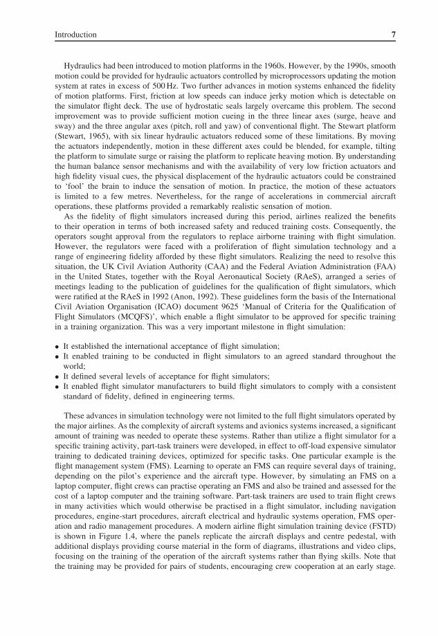
The aviation pioneers learned to fly by making short ‘hops’, progressively increasing the length ofthe ‘hop’ until actual flight was achieved (Turner, 1913). Training was mostly limited to advicegiven on the ground. There are a few examples of early training devices, but these were designedto enable pilots to experience the effects of the controls. The Sanders trainer (Haward, 1910),developed in 1910, comprised a cockpit which could be turned into the prevailing wind; if thewind was sufficiently strong, the cockpit would move in response to the pilot’s inputs. Similardevices were developed by Walters and Antionette (Adorian et al., 1979) in the same year, wheremotion of the cockpit was controlled by instructors, as shown in Figure 1.1.
During the First World War, flight training became established in dual-seat aircraft, notablythe AVRO 504 which was adopted as a basic trainer by the Royal Air Force (RAF) from 1916until 1933. The instructor demonstrated manoeuvres, which were practised by the student pilotuntil a satisfactory standard of proficiency was achieved to ‘go-solo’, with pilot and instructorcommunicating via a ‘Gosport speaking tube’. Despite the rapid advances in the early years ofaeronautics, the handling qualities of these aircraft were poor and many were unforgiving if flownbadly. It is claimed that more lives were lost in training1 than in combat during the First WorldWar (Winter, 1982).
By 1912, Sperry had developed rudimentary autopilot functions incorporating a gyroscope. In apublic demonstration in 1914, he flew a Curtiss flying boat ‘hands-off’ while a mechanic walkedalong the upper wing surface to the wing tip! By the late 1920s, flight instrumentation enabled pilotsto fly safely in cloud and rain, without visual reference to the ground. In instrument meteorologicalconditions (IMC), an artificial horizon, altimeter, airspeed indicator and a compass enabled pilotsto fly by reference to these instruments. Although the flying training syllabus had matured by the1930s, throughout this period the aircraft was accepted as the natural classroom for flight training,including training for instrument flying, with ground schools providing the theory to support flyingtraining.
In the late 1920s, Edwin Link, who is recognized as the founder of modern day flight simulation,developed a flight training device which enabled a significant part of instrument flying training to
1 In his book The First of the Few , Winter claims that 8000 of the 14,166 pilots killed in the First World War diedwhile training in the United Kingdom. In Parliament, on 20 June 1918, the Secretary of State attributed the lossesto the lack of discipline of the young pilots.
Principles of Flight Simulation D. J. Allerton 2009, John Wiley & Sons, Ltd

2 Principles of Flight Simulation
Figure 1.1 The Antionette flight training simulator circa 1911 (Courtesy: The Library of Congress)
be conducted in a ground-based trainer (Rolfe and Staples, 1986). Link worked in his father’sfactory in Binghamton, where they manufactured air-driven pianos and church organs. He had asound grasp of pneumatics and mechanisms and, having obtained a pilot’s licence in 1927, appliedhis knowledge of engineering to the construction of a flight trainer (Link, 1930), using compressedair to tilt the cockpit and to drive pressure gauges to replicate aircraft instruments. However, Linkexperienced considerable resistance to his ideas and initially sold his trainer (complete with a slotfor coins) to amusement parks.
Advances in aircraft design following the First World War saw a rapid expansion in aviation,including the delivery of freight and mail. The US Post Office subcontracted mail deliveries to theUS Army Air Corps. But in the early 1930s, they extended mail delivery to all-weather operations,leading to an alarming increase in fatalities. As a consequence, the US Army Air Corps purchasedsix flight trainers from Link, specifically for the task of instrument flight training – probably thefirst time that the value of flight simulation was recognized in flight training.
Link’s early contributions to flight training were fundamental:
• He exploited specific engineering technologies to produce a successful flight training device;• The flight trainer was developed to meet a specific training requirement;• Although his flight model was simple and inexact, the trainer was effective – it had a positive
benefit on pilot training;• The introduction of the Link trainer established the concept that flying training was not limited
to airborne training – effective training could also be undertaken in a ground-based trainer.
The problems of aircraft accidents occurring in instrument flight conditions resurfaced dur-ing the Second World War, with aircrews flying long distances in night-time operations and
Introduction 3
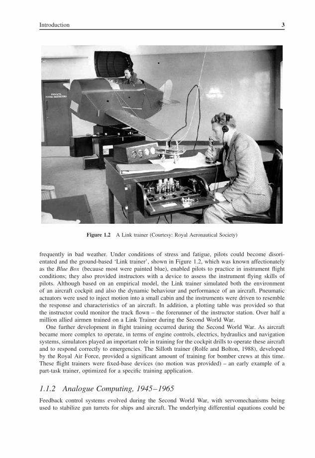
Figure 1.2 A Link trainer (Courtesy: Royal Aeronautical Society)
frequently in bad weather. Under conditions of stress and fatigue, pilots could become disori-entated and the ground-based ‘Link trainer’, shown in Figure 1.2, which was known affectionatelyas the Blue Box (because most were painted blue), enabled pilots to practice in instrument flightconditions; they also provided instructors with a device to assess the instrument flying skills ofpilots. Although based on an empirical model, the Link trainer simulated both the environmentof an aircraft cockpit and also the dynamic behaviour and performance of an aircraft. Pneumaticactuators were used to inject motion into a small cabin and the instruments were driven to resemblethe response and characteristics of an aircraft. In addition, a plotting table was provided so thatthe instructor could monitor the track flown – the forerunner of the instructor station. Over half amillion allied airmen trained on a Link Trainer during the Second World War.
One further development in flight training occurred during the Second World War. As aircraftbecame more complex to operate, in terms of engine controls, electrics, hydraulics and navigationsystems, simulators played an important role in training for the cockpit drills to operate these aircraftand to respond correctly to emergencies. The Silloth trainer (Rolfe and Bolton, 1988), developedby the Royal Air Force, provided a significant amount of training for bomber crews at this time.These flight trainers were fixed-base devices (no motion was provided) – an early example of apart-task trainer, optimized for a specific training application.
1.1.2 Analogue Computing, 1945–1965
Feedback control systems evolved during the Second World War, with servomechanisms beingused to stabilize gun turrets for ships and aircraft. The underlying differential equations could be

4 Principles of Flight Simulation
solved by electronic circuits. At the heart of these developments was the operational amplifier,constructed from thermionic valves. By providing a high gain amplifier with resistive feedback,signals could be summed algebraically and more importantly, by providing capacitive feedback, themathematical operation of integration could be applied to signals. These developments heraldedthe introduction of the analogue computer. Each amplifier could be configured as a summer orintegrator with gains implemented by potentiometers. Short wires were used to connect theseelements allowing complex sets of differential equations to be solved in real-time. The simplicity,relative low cost and capability of analogue computers to solve the equations inherent in nuclearpower generation, chemical reactions and electrical motor control established analogue computationas a major engineering discipline up to the mid-1960s.
In aeronautics, the analogue computer was used to model the equations of motion of aircraftdynamics (Allen, 1993) as sets of non-linear differential equations, giving the aircraft designer theopportunity to develop advanced control systems in the research laboratory. Indeed, the TSR-2 andConcord programmes made extensive use of analogue computers. Analogue computation offeredmajor advances: it enabled complex differential equations (including non-linear equations) to besolved; it offered real-time simulation; a program could be altered easily by changing the gain ofa potentiometer or by patching a few wires. However, this technology also had a number of majordrawbacks:
• The valves were unreliable and prone to drift, necessitating regular and complicated calibration;• The voltage range was limited – the equations had to be scaled manually in order to ensure that
the voltage range of the computer was not exceeded, without compromising the resolution ofvariables used in the computation;
• Multiplication and division of two variables was difficult and slow – mechanical multipliers andinverters were developed, but they lacked resolution;
• Non-linear terms, for example trigonometric functions were difficult to implement – resolvers,with predefined set-points were developed, but these elements were expensive and often limitedto a few linear segments.
Although analogue computation made a significant improvement to the fidelity of flight models,advances in motion systems and visual systems were much slower. These early simulators werelimited to simple motion drive platforms, often constrained to two or three degrees of freedom and,for the most part, were used to simulate instrument flight conditions. One significant developmentwas the provision of model boards, with very detailed scenery, where a camera was suspendedfrom a small gantry to follow the aircraft flight path over the terrain. The camera was mountedon a gimbal mechanism, allowing the camera to be synchronized with the flight model in pitch,roll and yaw. The camera video output was displayed on a monitor placed directly in front ofthe pilot, with the model board scaled exactly to the geometry of the pilot eye position. Althoughvery high levels of realism were achieved with detailed model boards, these systems had twopitfalls. First, the pilot could fly off the edge of the model board. One solution was to constructthe model board on a flexible base, passing over large rollers, so that the model board effectivelyrepeated. The second limitation was that the camera could collide with the model board, necessi-tating expensive repairs to the model board and even to the camera. These systems also providedendless opportunities for the prankster, for example, by placing a spider in front of the cameraduring finals.
There were two significant achievements during this period. First, airlines started to appreciatethe benefits of flight simulators, not only to reduce training accidents but also to reduce trainingcosts. Secondly, a significant industry developed in the United Kingdom and the United States tomanufacture flight simulators for airlines, notably Redifon and Link Miles in the United Kingdom.

Introduction 5
1.1.3 Digital Computing, 1965–1985
While analogue computers were used for real-time applications after the Second World War, digitalcomputers (developed from code-breaking devices) evolved more slowly, initially being introducedinto commercial applications, particularly data processing and payroll systems. During this period,the processing speeds advanced, early programming languages were developed and the capacity ofstorage devices increased. However, it was the development of the transistor in the mid-1960s thatinitiated the major advances in digital computation. By the 1970s, mini computers were used widelyfor scientific computing, evolving from the mainframe computers of the 1960s. As the processorspeeds increased, sufficient instructions could be executed to enable the equations of motion ofan aircraft to be solved at least 15 times per second (15 Hz). At rates below 15 Hz, delays in thecomputation can be perceived by human pilots, giving rise to unexpected or unusual responsesto pilot inputs. The early digital computers achieved this processing rate by using fixed-pointarithmetic rather than the slower floating-point arithmetic and by optimizing the code, typically byprogramming the equations in assembler code. However, by the late 1970s, the mini computerscould be programmed in a high-level language, using hardware floating-point processors to achievean update rate of 50 or 60 Hz. Indeed, several of the simulator companies developed their ownprocessors to meet the very demanding requirement of real-time processing, at this time.
As mini computers advanced in processing speeds, simulator manufacturers applied digital tech-nology to the development of visual systems with two notable achievements. First, with the use ofspecial-purpose hardware, light points defined in a scene could be transformed to the coordinatesof a cathode ray tube (CRT). With very fast response video amplifiers, the electron beam of a CRTcould be deflected to draw several thousand light points to provide a night or dusk scene. Notonly could the light points be rendered accurately, to provide a realistic night-time image, but theintensity of each light point could be modulated to simulate the effects of range or fog. The secondadvance came with projection. Up to this point, CRT displays were placed in front of the pilot.However, the image lacked realism; the pilot’s eyes were focused on the CRT screen, looking atpoints apparently several miles away. In addition, CRTs were much smaller than the windscreensof transport aircraft. After some experimentation with different lenses (including Fresnel lenses) thecollimated projector was introduced into airline simulators. The beams from a CRT reflected froma semi-silvered mirror onto a segment of a spherical mirror, passing back through the semi-silveredmirror to be seen by the pilot. This arrangement afforded two advantages:
• The image was magnified so that it was possible to fill an aircraft window with the image providedby a small CRT. The windows of a commercial transport aircraft are approximately rectangular,allowing the projection system to be mounted on the outside of the simulator cockpit – correctionfor optical distortion or reversal of the image was provided by adjustment to the CRT beamdeflection circuits;
• The light rays from the CRT seen by the pilot were almost parallel, producing an uncanny effectof distance (hence the phrase collimated).
Collimated projection systems were widely used from 1970 to the early 1990s. As monochromeCRTs gave way to colour CRTs to provide daylight images and the scene content increased withfaster graphics processors, the collimated projector had sufficient resolution and bandwidth to sustainthe 60 Hz frame rate provide by the image generators. However, these projectors had three inherentdisadvantages:
• Manufacturing an accurately machined curved mirror was expensive;• The weight of three or four mirrors added significantly to the (off-axis) load on the motion
platform;
6 Principles of Flight Simulation
• The image was only correct at the pilot eye-point – distortion increased away from the focalpoint of the projector mirror, to the extent that a pilot would be unable to see anything in thewindscreen in front of the other pilot.
1.1.4 The Microelectronics Revolution, 1985–present
Gordon Moore, one of the founders of the Intel Corporation, is widely attributed with encapsulatingthe advances of the microelectronics revolution in ‘Moore’s Law’ (Moore, 1965). By the 1980s,semiconductor companies were fabricating processors and memories as integrated circuits (ICs).Moore observed that the rate of progress was such that performance doubled with a fixed periodof time (and without a concomitant rise in cost), typically 18 months. In other words, every 18months or so, the capacity of memory chips or the processing speed of processor chips woulddouble, largely driven by a demanding and expanding domestic market for desktop PCs, computergames and audio and video equipment.
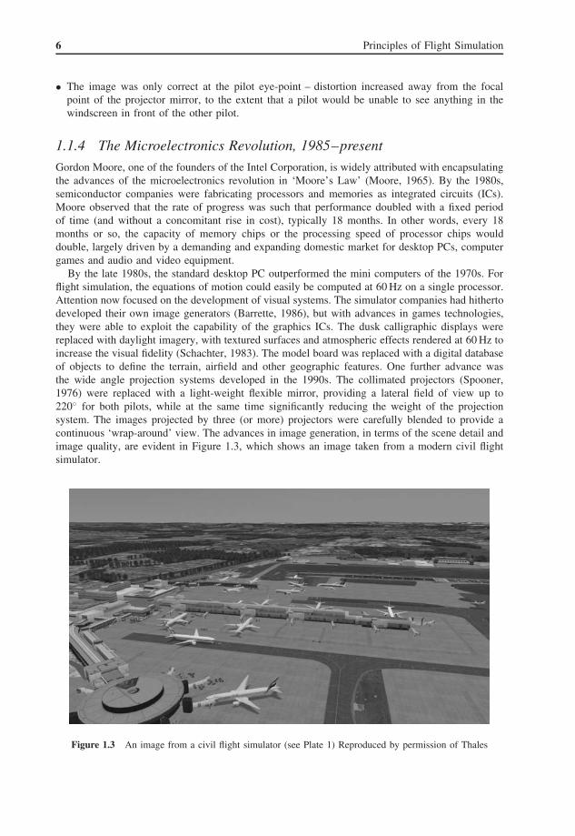
By the late 1980s, the standard desktop PC outperformed the mini computers of the 1970s. Forflight simulation, the equations of motion could easily be computed at 60 Hz on a single processor.Attention now focused on the development of visual systems. The simulator companies had hithertodeveloped their own image generators (Barrette, 1986), but with advances in games technologies,they were able to exploit the capability of the graphics ICs. The dusk calligraphic displays werereplaced with daylight imagery, with textured surfaces and atmospheric effects rendered at 60 Hz toincrease the visual fidelity (Schachter, 1983). The model board was replaced with a digital databaseof objects to define the terrain, airfield and other geographic features. One further advance wasthe wide angle projection systems developed in the 1990s. The collimated projectors (Spooner,1976) were replaced with a light-weight flexible mirror, providing a lateral field of view up to220◦ for both pilots, while at the same time significantly reducing the weight of the projectionsystem. The images projected by three (or more) projectors were carefully blended to provide acontinuous ‘wrap-around’ view. The advances in image generation, in terms of the scene detail andimage quality, are evident in Figure 1.3, which shows an image taken from a modern civil flightsimulator.
Figure 1.3 An image from a civil flight simulator (see Plate 1) Reproduced by permission of Thales
Introduction 7
Hydraulics had been introduced to motion platforms in the 1960s. However, by the 1990s, smoothmotion could be provided for hydraulic actuators controlled by microprocessors updating the motionsystem at rates in excess of 500 Hz. Two further advances in motion systems enhanced the fidelityof motion platforms. First, friction at low speeds can induce jerky motion which is detectable onthe simulator flight deck. The use of hydrostatic seals largely overcame this problem. The secondimprovement was to provide sufficient motion cueing in the three linear axes (surge, heave andsway) and the three angular axes (pitch, roll and yaw) of conventional flight. The Stewart platform(Stewart, 1965), with six linear hydraulic actuators reduced some of these limitations. By movingthe actuators independently, motion in these different axes could be blended, for example, tiltingthe platform to simulate surge or raising the platform to replicate heaving motion. By understandingthe human balance sensor mechanisms and with the availability of very low friction actuators andhigh fidelity visual cues, the physical displacement of the hydraulic actuators could be constrainedto ‘fool’ the brain to induce the sensation of motion. In practice, the motion of these actuatorsis limited to a few metres. Nevertheless, for the range of accelerations in commercial aircraftoperations, these platforms provided a remarkably realistic sensation of motion.
As the fidelity of flight simulators increased during this period, airlines realized the benefitsto their operation in terms of both increased safety and reduced training costs. Consequently, theoperators sought approval from the regulators to replace airborne training with flight simulation.However, the regulators were faced with a proliferation of flight simulation technology and arange of engineering fidelity afforded by these flight simulators. Realizing the need to resolve thissituation, the UK Civil Aviation Authority (CAA) and the Federal Aviation Administration (FAA)in the United States, together with the Royal Aeronautical Society (RAeS), arranged a series ofmeetings leading to the publication of guidelines for the qualification of flight simulators, whichwere ratified at the RAeS in 1992 (Anon, 1992). These guidelines form the basis of the InternationalCivil Aviation Organisation (ICAO) document 9625 ‘Manual of Criteria for the Qualification ofFlight Simulators (MCQFS)’, which enable a flight simulator to be approved for specific trainingin a training organization. This was a very important milestone in flight simulation:
• It established the international acceptance of flight simulation;• It enabled training to be conducted in flight simulators to an agreed standard throughout the
world;• It defined several levels of acceptance for flight simulators;• It enabled flight simulator manufacturers to build flight simulators to comply with a consistent
standard of fidelity, defined in engineering terms.
These advances in simulation technology were not limited to the full flight simulators operated bythe major airlines. As the complexity of aircraft systems and avionics systems increased, a significantamount of training was needed to operate these systems. Rather than utilize a flight simulator for aspecific training activity, part-task trainers were developed, in effect to off-load expensive simulatortraining to dedicated training devices, optimized for specific tasks. One particular example is theflight management system (FMS). Learning to operate an FMS can require several days of training,depending on the pilot’s experience and the aircraft type. However, by simulating an FMS on alaptop computer, flight crews can practise operating an FMS and also be trained and assessed for thecost of a laptop computer and the training software. Part-task trainers are used to train flight crewsin many activities which would otherwise be practised in a flight simulator, including navigationprocedures, engine-start procedures, aircraft electrical and hydraulic systems operation, FMS oper-ation and radio management procedures. A modern airline flight simulation training device (FSTD)is shown in Figure 1.4, where the panels replicate the aircraft displays and centre pedestal, withadditional displays providing course material in the form of diagrams, illustrations and video clips,focusing on the training of the operation of the aircraft systems rather than flying skills. Note thatthe training may be provided for pairs of students, encouraging crew cooperation at an early stage.

8 Principles of Flight Simulation
Figure 1.4 A flight simulation training device (FSTD) (see Plate 2) Reproduced by permission of Thales
One other role for flight simulation during this period has been to support engineering design(Allerton, 1999). The cost of flight trials of new equipment and aircraft systems is very expensiveand flight simulation has enabled engineers to design and evaluate aircraft systems. Errors eliminatedin the design phase are much less costly to rectify than at the flight trials stage. In addition,the simulator provides the designer with much more insight into ‘what-if’ studies, enabling thedesigner to compare prototype designs before committing to aircraft equipment. Consequently,the emphasis of flight trials has shifted towards the validation of data derived in simulator studies,rather than expanding the flight envelope. In both the Boeing 777 and the Airbus A380 programmes,engineering simulation made a major contribution to the design of these aircraft.
Since 1985, flight simulation has had a major impact in military flight training. It is arguablethat flight simulation was introduced too early into military flight training, giving rise to the viewthat military flight training was more effective in an aircraft. This argument was further reinforcedby the lack of fidelity of flight trainers in the 1960s, giving simulation a bad reputation in manymilitary organizations.
As the cost of training came under strict scrutiny and environmental issues became more promi-nent, military organizations reviewed the benefits that had been achieved by civil flight trainingorganizations and simulation became an integral part of flying training programmes throughout theworld. However, the technology of civil flight training is not appropriate to all military trainingprogrammes. In particular, the pilot of a fighter aircraft is not constrained to a forward lookingwindscreen and during turning manoeuvres, the sustained G-force cannot be replicated with a con-ventional motion platform. Two advances have, to a limited degree, ameliorated these problems.The motion platform has been replaced with a G-seat in a fixed-base cockpit (White, 1989), to pro-vide more effective training (Ashworth, 1984). As the pilot is subject to G-forces, actuators controlthe tightness of the harness and provide tactile cues to exert additional pressure on the pilot’sbody. In addition, the buffet experienced in combat manoeuvres near to the stall limit is provided
Introduction 9
by vibration of the seat assembly. Two solutions have been developed to provide a pilot with a360◦ field of view. In some simulators, the pilot’s helmet is instrumented to detect head and eyemovement. The image is derived from the eye and head position and is projected directly onto thepilot’s eye by a small optical system mounted on the front of the helmet. An alternative approachis the hemispherical dome, used in conjunction with an array of conventional projectors to projectthe terrain (at relatively low resolution) and several laser projectors to provide high-detail imagery(e.g. aircraft in the scene). The cockpit is placed at the centre of the dome and the projectors arepositioned near the base of the cockpit, giving the pilot an all-round view.
One particular area of success in military simulation has been mission rehearsal. By generatingthe visual database of a combat area (typically derived from satellite mapping), flight crews canrehearse a mission in a flight simulator, even to the extent of applying lessons learnt in the simulatorto the mission. Military simulators are also linked via high speed networks to enable flight crewsto practise multi-ship missions, either to test tactical manoeuvres against each other or to practisetactics for a specific mission.
1.2 The Case for SimulationNowadays, the use of flight simulation in both civil aviation and military training is commonplaceand widely accepted (Allerton, 2000). These simulators allow flight crews to practice potentiallylife-threatening manoeuvres in the relative comfort of a training centre. Similarly, military pilotsare able to rehearse complex missions and to practise piloting skills that may be unacceptablein environmental terms (in peace time) or prohibitively expensive, for example, the release ofexpensive weapons.
1.2.1 Safety
Aviation is underpinned by safety. The primary role of the aviation authorities is to ensure the safetyof all aircraft operations, including flight training. As recently as the 1970s, airlines would trainwith actual aircraft, practising circuits, takeoffs and landings and even simulate system failures.Unfortunately, there were a significant number of training accidents and one major benefit of flightsimulation has been to eliminate these accidents.
An airline pilot undergoes two days of training and checking every six months. Quite probably,if pilots had been asked in the 1960s if they would be prepared to renew their licence in a simulator,there would have been universal reluctance to consider such an option. Nowadays, if pilots wereasked to undertake this training in an aircraft, there would be a similar rejection of the suggestion.
This is a remarkable transition in a very short time and is simply attributable to the technicaladvances in modelling, visual systems and motion systems. Flight simulation is accepted by thepilots, operators, unions, regulatory authorities and manufacturers. Indeed, some simulators arequalified for zero flight-time (ZFT) training. With these flight simulators (and an approved flighttraining organization), all the conversion training is undertaken in a ZFT flight simulator. The firsttime the pilot will fly the aircraft is with fee-paying passengers on a scheduled flight. Of course,the pilot will be closely monitored by a training captain, but it reflects the advances and acceptanceof simulation technology throughout the world.
One further aspect of flight safety is reflected by air accident statistics. Following an accident,the regulatory authorities and airlines will study the report of the air accident investigators and mayrequire airlines to incorporate similar events in their training programmes to enable flight crews tobe aware of similar situations. The flight simulator allows pilots to experience a very wide range offlight conditions, so that a pilot will have experienced situations in a simulator within the last sixmonths that most pilots would not normally encounter in their full career. The crew of the Apollo 13mission attributed their success in coping with the malfunctions on their mission to the many hoursspent in a simulator, rehearsing the hundreds of possible flight situations they might encounter.
10 Principles of Flight Simulation
With the increase in air traffic since the 1970s, flight simulation has made a major contribution toincreased flight safety. In particular, flight simulation accelerates experience. In the flight simulator,the instructor can select fog, turbulence, wind-shear or icing conditions in a couple of touch-screeninputs. In normal operations, a pilot might only experience specific wind-shear once in five years.Indeed, with extended operations and four pilots per sector, airline pilots can struggle to completesufficient manual landings to remain current. In such situations, landings practised in a flightsimulator are accepted by the regulatory authorities. One future role for flight simulation may beto maintain the proficiency of pilot handling skills.
In the 1970s, a number of regulators and airlines recognized that a significant proportion ofair accidents and incidents were attributable to pilot error, particularly in multi-crew operations,where communications between flight crew or the management of situations broke down. The flightsimulator provided the ideal platform to practise crew cooperation procedures and to improve thetraining of flight crews to respond to hazardous situations. In many training organizations, the flightcrew response is recorded and reviewed in debriefing sessions. Lessons learnt from the analysis ofcockpit flight data recorders and cockpit voice recorders, following aircraft incidents and accidents,have been incorporated in simulator training programmes. It is probable that the aviation industryhas led the world in the use of simulation technology to improve training and safety.
1.2.2 Financial Benefits
A wide body transport aircraft typically has eight flight crews per aircraft and one flight simulatorper eight aircraft. With 128 pilots requiring four days flight training per year (four 8-hour shifts),simulation utilization approaches full capacity, without allowing for type conversion programmesfor flight crews joining the airline or converting onto type. With airborne operations at least 10times the cost of simulator operations, the cost of equivalent airborne training would bankrupt anairline. There is a strong case that flight simulation has enabled budget airlines to grow and that,without flight simulation, they would not be able to operate.
The major costs of flight training include:
• The cost of purchasing the flight simulator;• The cost of building the simulator facility;• The running costs of the simulator facility (electricity, air conditioning, computer maintenance,
spares provision, etc.);• The staff costs to provide flight training and maintenance of the simulator (instructors, mainte-
nance engineers, administrators, etc.).
The income to a simulator organization comes from selling training time on the simulator.Typically, flight simulators operate 23 hours per day and over 360 days per year. Assuming thesimulator and the training organization have the appropriate approvals, the role of the simulatormanager is to ensure utilization of the simulator and optimize the income.
In addition to the day-to-day operation of a simulation facility, the procurement of a simulatorcan also affect the financial return. First, there is a lead-time of the supply of both aircraft andsimulators to an airline. An airline will procure specific aircraft for its route structure and then trainits pilots to operate these aircraft. Balancing the number of simulators to aircraft types is difficultas route structures can change. Secondly, delays in construction of the building, the delivery ofthe aircraft or delivery of the simulator can cause a significant loss of revenue. Revenue can begenerated by selling spare capacity to other operators. Alternatively, a lack of availability mayrequire pilots travelling to train on simulators operated by other airlines. Thirdly, the long leadtimes can result in variation of bank rates (for loans) or changes in customer markets.
Clearly, these are tightly balanced financial equations for any simulator operator. However,many of the operational costs are fixed (such as instructor salaries and electrical consumption).

Introduction 21
three channels covering a total of 180◦, the forward channel is offset by 0◦ and the other channelsare offset by –60◦ and +60◦. In practice, the projected channels overlap by a few degrees, to avoidany visible gaps in the projected image. Strictly, two pilots seated at the front of an aircraft wouldnot see identical views. In practice, the angular differences are small and are ignored. The imageformed by the image generator is generated as a 2D image, in effect for a flat screen. If this imageis projected directly onto a curved screen, it will appear distorted. To ensure correct geometry in theprojection, as viewed at the pilot eye-point, the distortion of the image is corrected in the projectorcircuitry. This alignment is set up during installation and is checked regularly during maintenanceschedules.
1.4.8 Sound System
The aircraft cockpit or flight deck is a noisy environment. Pilots hear a wide range of soundsincluding slipstream, engines, sub-systems, air conditioning, ground rumble, actuators, radio chat-ter, navigation idents, warnings, weapon release and alarms. Although sounds are provided in asimulator to increase fidelity, they are also important cues and they must be consistent with thesounds heard in an aircraft.
Some sounds, such as airspeed or engine revolutions per minute (RPM), vary with flight con-ditions whereas other sounds give a constant tone (or set of tones), for example, a fire warning.Usually, a separate sound system is provided, taking inputs from other modules, for example, engineRPM from the engine module, slipstream magnitude from the flight model or marker ident fromthe navigation module.
Generally, two methods are used to generate cockpit sounds. The obvious technique is to recordactual aircraft sounds, using a high quality sound recording system placed in the cockpit or flightdeck, typically with a microphone suspended from the roof of the cabin. The drawback with thisapproach is the number of recordings needed to cover all flight conditions. For example, enginesounds vary with airspeed, altitude and engine state (RPM and thrust) and it would be necessaryto cover the full range of these variables. The recordings are then accessed every frame to outputa small fragment, 1/60th of a second at 60 Hz. The sound signals must also be continuous – anydiscontinuities between frames would result in interference which would be detectable. Althoughmany commercial sound cards are designed to replay recorded sounds, there are in excess of 50separate sound components which need to be generated and combined every frame.
The alternative method, and the one more commonly adopted, is to analyse the source of eachsound and generate the appropriate waveform. For simple sounds, such as a warning alarm, thisis straightforward as these sounds comprise a set of tones. The sound of jet engines, propellersand rotors are more complicated. Nevertheless, the fundamental frequencies of these noise sourcescan be identified and combined with different forms of white (i.e. random) noise. In effect, eachsound consists of several components and for each sound, these components are computed as afunction of its primary variables every frame. With earlier sound cards, synthesizer ICs were usedbut nowadays the sound waveform can be generated by a digital signal processor. One furtherattraction of this method is that synthetically generated sounds can be compared with actual aircraftsounds to confirm the authenticity of the generated sound, typically by applying a fast Fouriertransform (FFT) to the respective sounds and comparing the frequency spectra.
1.4.9 Motion System
As the simulated aircraft is manoeuvred, the pilot will expect to feel the accelerations that wouldbe experienced in actual flight. The accelerations are computed in the flight model and are passedto the motion system. For the standard motion platform comprising six linear hydraulic actuators,each actuator is moved to a new position to try to replicate the accelerations on the pilot’s body.

22 Principles of Flight Simulation
Very fast response actuators are used and these are updated at rates in excess of 500 Hz to eliminatejerkiness in the motion.
Of course, true motion cues cannot be generated. For example, a military aircraft can fly a 4Gturn for several minutes whereas the only positive G available from the platform is vertical heave,which is constrained by the length of the hydraulic actuators (typically 2–3 m). Similarly, in arolling aerobatic manoeuvre the pilot is subject to lateral accelerations and angular moments. Thearrangement of the legs of the platform restricts angular motion to 30–40◦. However, the humanmotion sensors and the brain can be fooled. The brain responds to the onset of motion but cannotdetect very low rates of motion, so that motion can ‘leak away’ without the pilot realizing thatmotion has changed. In addition, if the motion cues are reinforced with strong visual cues by thevisual system, the pilot can sense motion that is not actually applied to the platform. In some fixedbase simulators, the motion sensed from visual cues can convince pilots that the simulator has amoving platform. Indeed, there are (undocumented) instances where the motion system has beenswitched off without the flight crew realizing that motion cues had been suppressed.
The motion system contains computers to derive the actuation equations to move the platform tothe desired position, together with filters to optimize the platform trajectory and provide appropriatemotion for the pilot’s balance sensors. Of course, this is a compromise and moreover, differentpilots have different perceptions of motion. However, assessment of the motion is a very importantaspect of simulator qualification and is checked for critical phases of flight, particularly takeoff,landing and engine failures.
One final and important consideration for the motion platform is safety. The cabin could fallseveral metres under active control, as a result of a system failure, causing injury to the occupants.Redundant computer systems and extensive monitoring is used to detect unexpected motion, shuttingdown the hydraulic actuation within a few milliseconds to avoid any injury, if any undesired motionof the platform is detected. One other aspect of safety is that the platform is 4–5 m off the ground.In the case of a fire or emergency, the hydraulic system should lower the platform to its lowestpoint to allow the flight crew and instructor to escape via ladders.
1.4.10 Control Loading
As an aircraft flies, the slipstream passing over the control surfaces changes the load on thesesurfaces, particularly the primary flight controls: the elevator, aileron and rudder control surfaces.The force per unit displacement increases (non-linearly) with airspeed and affects the handling ofan aircraft. Such effects must also be simulated and this is the function of the control loadingsystem. Control loading is provided by attaching actuators to the flight controls in the simulator sothat the actuator provides resistance to motion, typically varying with airspeed.
Prior to 2000, most simulators used hydraulic actuators for control loading. By driving the actua-tor with a computer system, the control loading system can be programmed to emulate springiness,damping, end stops, backlash and dead bands. The characteristics of hydraulic actuation are sogood, that an emulated mechanical end stop feels as though the control column is in contact with amechanical end stop. Since 2000, advances in electrical motor drives have enabled control loadingto be implemented with a single motor drive per channel. Control loading is also an important partof simulator qualification and there have been concerns that residual torques can be detected aroundthe centre position, at very low values of torque where electrical systems lack response. With bothhydraulic and electrical control loading systems, the trimming function is simply implemented asa null datum offset for the zero load position. To provide force feedback for the control columnor centre stick, the inceptor displacement is sensed using an LVDT or stick force is measured bymeans of a strain gauge.
Both hydraulic and electrical control loading systems must meet strict safety requirements. Acontrol column, some 12 in. in front a pilot could cause considerable harm if accidentally driven at
Introduction 23
full power towards the pilot. Similarly, an auto-throttle lever quadrant has the potential to sever apilot’s fingers if moved unexpectedly. Consequently, the applied forces of control loading systemsare very closely monitored by separate systems, which can remove any control loading within afew milliseconds.
1.4.11 Instrument Displays
Aircraft instruments cover two eras of flight. Prior to 1980, most aircraft had mechanical instru-ments. Many of these instruments had complicated mechanisms, including multiple pointers, rotatingcards, digital readout and clutch mechanisms. Since 1980, many civil and military aircraft havemoved to electronic flight instrument systems, known as EFIS displays . These EFIS displays arebased on computer graphics with 8-in. ruggedized monitors, typically with the displays updatingat least 20 times per second (20 Hz). The graphics hardware in the display has a very fast drawingspeed to sustain the frame rate and includes anti-aliasing algorithms to smooth any jagged lines oredges as characters and lines are rendered.
The conventional mechanical displays have been implemented since the Link trainer, initiallyusing mechanically driven pointers or using pneumatics to drive adapted pressure gauges. Nowa-days, simulated instruments are driven by servo motors or stepper motors, using specializedmechanisms to provide all the functionality of aircraft instruments, for example, the fail flags of aVOR instrument or the barometric pressure setting for an altimeter. Such instruments are driven byanalogue voltage via an I/O card. Many of these instruments contain complex mechanisms to driveseveral pointers, rolling digits, rotating compass cards and clutch mechanisms for pilot settings.Consequently, with older simulators, these mechanical instruments are often unreliable, requiringregular inspection and maintenance.
With EFIS displays, the simulator manufacturer has the option of using the original aircraftequipment. Alternatively, a modern processor with a low performance graphics card is capable ofemulating the EFIS displays found on most aircraft. This option is sometimes referred to as the stim-ulate or simulate debate; either original equipment is stimulated, but the simulator must provide thecorrect input signals or the equipment is simulated, but then the simulator manufacturer must ensurethat all the possible operating modes and functionality have been correctly implemented. In terms ofcost, the latter option (in effect, reverse engineering) is generally preferred by simulator developers.
For military aircraft, and more recently for some civil transport aircraft, the simulator may alsorequire a head-up display (HUD). If the original aircraft equipment is used, the appropriate videosignal format must be generated for the HUD. Actual HUDs are collimated so that the imageappears to be overlaid on the outside world. The optical attenuation is small, so that the externalworld can be seen through the HUD together with the flight data optically projected via a CRT. Oneoption is to place a small monitor in front of the pilot, combining both 2D graphics (the HUD) with3D graphics aligned to the projection system. However, such systems can give rise to pilot fatigueas the focal length varies between looking at the HUD and looking at the projected image. Thisproblem can be overcome by projecting the HUD information as a graphical overlay on the visualsystem; in this case, the pilot simply looks through an open frame representing the HUD frame.This method has the advantage that the pilot does not need to accommodate the HUD informationas it is effectively focused at infinity. On the other hand, slight movement of the pilot’s head cancause information on the HUD to appear outside the HUD frame.
1.4.12 Navigation Systems
A significant part of flying training covers navigation training. Flight simulation offers two advan-tages: first, an airborne navigation exercise consumes fuel and secondly, navigation errors in trainingcan be hazardous. Consequently, simulators provide varying degrees of navigation capability. For

24 Principles of Flight Simulation
instrument approaches, VOR, automatic direction finding (ADF) and ILS systems are emulated.This requires integration with radio management panels or an FMS to select receiver frequenciesand an up-to-date database of navigation aids. In addition, the errors associated with these systemsmust be modelled correctly. For example, a VOR operates in the very high frequency (VHF) bandand therefore is line-of-sight; it can fail if the aircraft is too low to receive the signal or if thetransmitter is obstructed by a hill. Similarly, false glide slope indications, common at some ILSinstallations, need to be modelled.
For enroute navigation, VOR, inertial navigation systems (INS) and the Global Position System(GPS) are also simulated. In addition to simulation of the correct functionality, it is important tomodel the error properties of these systems. For example, an INS will drift and exhibit the slow‘Schuler loop’ oscillation. Similarly, GPS accuracy varies with the geometric dilution of precision(GDOP) caused by variations in the GPS satellite constellation. In an aircraft, these navigationsystems are integrated with the FMS and flight displays (typically via the aircraft databus) andsuch functionality must be replicated in the simulator, particularly the appropriate behaviour forthe relevant failure modes.
For short-range navigation, a ‘flat earth’ model may be adequate for navigation. Beyond rangesof 100 miles or so, a full spherical earth model is needed for navigation, transforming the aircraftmotion to earth latitude and longitude axes. For longer distances, Coriolis acceleration terms (theeffect of earth rotation on perceived motion) need to be modelled.
1.4.13 Maintenance
In addition to the systems outlined above, the simulator must be regularly checked to ensure thatit is operating within limits. Indeed, for qualified simulators, the operator must keep a log of allscheduled and unscheduled maintenance and repeat diagnostic tests to confirm that the simulatorcharacteristics have not changed significantly, following any maintenance procedures.
Specific tests are conducted for all the sub-system modules. If the module contains a processoror memory, these will be exercised and tested for failures. The visual system and projection systemwill be checked for alignment, where patterns of rectangles and dots are used to detect drift in theoptical systems. Light levels and grey scales are also checked for illumination intensity, togetherwith variation in colour bands for the red, blue and green components, often caused by ageing ofthe projector bulbs.
For mechanical systems, tests are made for excessive wear or increased friction. Such testsare typically computer-based, where tests are initiated and the results compared with results fromprevious bench-mark tests. In addition to problems with wear in actuators, sensors may also fail,with ingress of dirt or hydraulic fluid contamination. When sensors or actuators are replaced,extensive diagnostic software is run to check the sensor: that it operates over its full range, that ithas been reconnected correctly and that there is no discontinuity or noise on the sensor input.
In airline flight simulators, the simulator usage is constantly monitored and recorded. Usage isan important issue. If, for example, a simulator has been subjected to heavy landings, large jolts canaffect the visual system mirror or reduce the life of projector bulbs or motion platform bearings. Allfaults are logged and at the end of a training session, the instructor can report any malfunctions oranomalies that occurred during the session. Moreover, to guarantee over 95% availability, the airlinewill have technical support teams, with specialized knowledge of the simulator modules, to providefast response to any failures or problems and a large inventory of spares to minimize any down time.
1.5 The Concept of Real-time SimulationIn normal everyday life, everything seems to be continuous and instantaneous. The motion of a caralong a road is continuous; a ball follows a smooth trajectory through the air; a tree branch waves

Introduction 25
smoothly in the wind. Of course, we are not strictly solving any equations nor is a tree computingthe positions of all of its branches.
Computation is a very different world. We write software programs and the computer executesthe instructions of the program. These instructions may involve additions of machine registers,comparing memory locations and jumping from one address in the computer memory to anotheraddress. However, each of these instructions takes a finite number of machine cycles and each ofthese cycles is clocked at the speed of the processor. In other words, for a given computer, a smallfragment of code may take several microseconds to execute. This time may also vary dependingupon the program and its data. For example, to sort 100 numbers may take much longer than sorting20 numbers.
Anyone using a computer for office activities is subject to these delays. For example, spellchecking a document may take several seconds for a large section of text. The computer has toload its dictionary of words, access the file containing the text and then search for each word inthe dictionary. These operations may require several million computer instructions, but generally, auser is not too concerned whether it takes two seconds or three seconds to spell check a document.Of course, if it took five minutes, we might seek an alternative solution (e.g. a better algorithm ora faster computer or a faster disk).
There is one area of office computing where we might notice even small delays. If we movethe mouse we expect the cursor to move instantly over the screen, or if we press a key, we expectthe appropriate character to appear on the screen. In this case, there is a human in-the-loop andwe would expect a response within 1/10th of a second, anything less would be intolerable to theaverage computer user.
Consider an example where the user moves the mouse around the screen. The computer is, ineffect, executing the following code:
Check to see if the mouse needs redrawing, and if so
read the new mouse position
compute the screen coordinates (x, y) of the mouse
erase the cursor at its current position
draw the cursor at (x, y)
For each of these actions, a set of computer instructions is executed, but if the computer canexecute 107 instructions per second, say, then if we only need 10,000 instructions for this code,the software will be executed in 1 ms – from the human perspective, instantaneously. However, onan older computer, the same number of instructions might take 100 ms (or 1/10th of a second) andwe might discern a slight jerky motion of the mouse.
Of course, an office computer may be executing other tasks, such as printing a file and therefore,it will need to suspend the printing task frequently to check the mouse for movement. If themouse handling task is serviced 50 times per second, the cursor will appear to move smoothly inresponse to the mouse input. However, if the computer is occupied with other tasks, so that themouse is only serviced twice a second, the mouse will seem unresponsive or slow. Generally, officeoperating systems provide acceptable mouse management and the mechanism to ensure that themouse software is activated 50 times per second is part of the operating system and is transparentto the user.
What the operating system does is to discretize time, into very small time steps, so that themouse management code is guaranteed to be executed 50 times per second. These time steps aresmaller than we can discern with our eyes (and hand and brain), giving the mouse what appears tobe instantaneous and continuous motion, although it is actually implemented at discrete intervals.Of course, we are all used to such systems; television cameras at a football match capture framesevery 1/25th of second, which are transmitted to the television in a house. Because the time step
26 Principles of Flight Simulation
is so small, it appears that the players on the pitch are moving in the normal continuous way thatwe would expect to see if we sat in the stand at the match.
Exactly the same situation occurs in flight simulation. In an aircraft, the pilot moves the controlcolumn. Assuming direct cable linkage to the control surfaces (and ignoring the inertia of thecontrol surface), the elevator moves immediately, causing a perturbation to the aircraft, which isseen as a change in pitch by the pilot who responds with another movement of the control column tocorrect the pitch attitude. In a flight simulator, the stick position is sampled, the elevator deflectionis computed, a new pitch attitude is computed and an image is displayed by the visual systemwith the new pitch attitude, enabling the pilot to correct the aircraft attitude. The important point isthat the overall time for this computation must be sufficiently short so that it appears instantaneousto the pilot. In a modern simulator, these computations must be completed within 1/50th of a secondor 20 ms.
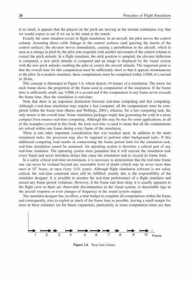
This concept is illustrated in Figure 1.6, which depicts 10 frames of a simulation. The arrow foreach frame shows the proportion of the frame used in computation of the simulation. If the frametime is sufficiently small, say 1/50th of a second and if the computation in any frame never exceedsthe frame time, then the simulation is real-time.
Note that there is an important distinction between real-time computing and fast computing.Although a real-time simulation may require a fast computer, all the computations must be com-pleted within the frame time (Burns and Wellings, 2001), whereas, for a fast computing task, theonly metric is the overall time. Some simulation packages imply that generating the code in a morecompact form ensures real-time computing. Although this may be true for some applications, in allof the examples covered in this book, the term real-time is used to mean that all the computationsare solved within one frame during every frame of the simulation.
There is one other important consideration that was touched upon. In addition to the mainsimulation tasks, the processor may also be required to perform other background tasks. If thisadditional computing load results in contravening the frame period limit for the simulation task,real-time simulation cannot be sustained. An operating system is therefore a critical part of anyreal-time simulator. The operating system must guarantee that it will execute the simulation taskevery frame and never introduce delays that cause the simulation task to exceed its frame limit.
In a safety critical real-time environment, it is necessary to demonstrate that the real-time framerate can never be violated beyond any reasonable level of doubt (which may be never more thanonce in 107 hours, or once every 1141 years). Although flight simulation software is not safetycritical, the real-time constraint must still be fulfilled; usually this is the responsibility of thesimulator designer. It is possible to monitor the real-time performance of a flight simulator andrecord any frame period violations. However, if the frame rate does drop, it is usually apparent tothe flight crew as there are observable discontinuities in the visual system, or discernible lags inthe aircraft response or even changes of frequency in the sound system outputs.
The simulator designer has, in effect, a time budget to complete all computations within the frameand consequently, tries to exploit as much of the frame time as possible, leaving a small margin forerror in these estimates (or for future expansion), particularly as some computation times are data
1 2 3 4 5 6 7 8 9 10 Frame
Figure 1.6 Real-time frames

Introduction 27
dependent. Given all the constraints on the scene content of the visual system, the processing ofthe flight model, the engine model, the weather model and so on, it is not uncommon for the frameperiod to be exceeded occasionally, even for a full flight simulator, particularly as the simulatormanufacturer may not have full control over the behaviour of a graphics card under all flightconditions. Nevertheless, ensuring real-time performance, particularly for worst-case conditions isan essential part of system validation and acceptance tests.
1.6 Pilot CuesA pilot in an aircraft perceives the sensation of flight from the stimulation of the pilot’s senses. Ofcourse, these are the same sensors we use in everyday life. They have evolved over millions of yearsand are optimized for survival. For example, we can perceive the colour, size and distance of a caron a motorway using our visual sensors or run down an escalator using our balance sensors. In flightsimulation, these stimuli are referred to as cues and, if we are to provide the same sensation of flightin a simulator, it is necessary to provide the same cues as those detected in flight. It is thereforeimportant to understand the cues we use in flight and also the mechanisms in the human body todetect these cues. In addition, if it is not possible to provide the same cues, an understanding of thesensors of the human body and the priority attached to specific cues in processing these cues, mayenable the simulator designer to reduce or simplify the cues that need to be provided in a simulator.
The issue of fidelity was discussed briefly in Section 1.2.3. The AGARD (Advisory Groupfor Aeronautical Research and Development) Flight Mechanics Panel observed in their report on‘Fidelity of Simulation for Pilot Training’ (AGARD, 1980) that ‘The degree of realism requiredof the simulation will depend upon the nature of the training task, the level of experience of thestudents and the level of proficiency they are required to attain’. In reducing fidelity, care is neededto ensure essential cues are not omitted, while on the other hand, considerable savings can be madeif unnecessary cues can be eliminated.
There are four stimuli we perceive as humans:
• Chemical – particularly smell and taste – generally, these do not need to be provided for flightsimulation;
• Thermal – temperature – for most simulators, the ambient operating temperature of the flightdeck or cockpit is sufficient;
• Photochemical – brightness and colour detected by the eyes;• Mechanical – these include auditory sensors to detect sounds, vestibular sensors to detect gravity
and angular and translational motion, kinaesthetic sensors to detect the position and movementof joints and pressure applied to the body and tactile sensors to detect pressure on the skin.
In addition to these sensors, the brain provides a fusion function, combining and processinginformation to provide the pilot with an understanding of position, orientation, speed and accelera-tion in the environment. This is an important consideration for the flight simulator designer; it mayallow one stimulus to be substituted for another. For example, motion is sensed by cues provided bythe visual system (the eyes) and by the motion platform (the vestibular system) offering a potentialtrade-off of visual cues against motion cues. These stimuli also have different paths through thenervous system of the human body and necessitate different amounts of processing by the brain.Consequently, the brain is able to compensate for these delays. However, if these delays are dif-ferent in a simulator (e.g. the response of instruments, the visual system or the motion platform toa pilot input), then this can lead to an unacceptable ‘feel’ of the simulator and in extreme cases,even lead to anxiety resulting in sweating and nausea (the so-called simulator sickness).

28 Principles of Flight Simulation
1.6.1 Visual Cueing
Visual cues (Buffet, 1980) are sensed by the eye. With two eyes, binocular vision provides furtherinformation of size and distance. The characteristics of the human eye are summarized in Table 1.2.
Note that, for a projection system with a lateral field of view of 180◦, acuity of 1 arc minute cor-responds to 1 part in 10,800. Assuming that three projectors are used, with each channel providing1000 pixels laterally (allowing for overlap), then current image generators and projectors need toincrease resolution by a factor of almost four, to achieve images that correspond to the acuity ofnormal vision, implying an increase by a factor of 16 of the pixel rendering rate.
The external world seen by a human observer covers the region within touch (1 m) of theobserver, the immediate vicinity (up to 30 m), where there is considerable detail and the likelihoodof dynamic objects and the far field (beyond 30 m), which is remote and provides a stable 3Denvironment. The human observer acquires different information in these three regions to perceiveimages, distance and movement (Farmer et al., 1999).
We perceive images by recognizing familiar shapes, for example, a tank with a turret and barrelwould be recognized over a wide range of distance and in different orientations. The brain is combin-ing colour and knowledge – basing its decision-making on the expected image, not necessarily theactual image. In other words, the context in which an image is generated will affect its credibility.For example, in a desert scene, an acceptable tank might be generated by a few hundred polygons,whereas in an urban scene, more detail may be necessary to provide an acceptable image of the tank.
We perceive depth in several ways. Muscles in the eye are used to focus on an object. Othermuscles in the eyes converge both eyes to provide a single image (binocular vision). The brain isalso able to process the different images formed on the retinas to provide further depth perception.From knowledge of the external world, occlusion (one object in front of another object) and relativesize of objects provide important depth cues. In other words, depth might be emphasized by thepositioning of objects in the environment. We are used to seeing perspective cues, such as a railwayline converging in the distance to provide depth cues. In a simulator, the arrangement of fields mightprovide useful depth cues in comparison with a more bland landscape. Also, objects placed on theground appear higher in the visual field towards the horizon. Accordingly, known objects on the
Table 1.2 Characteristics of the human eye
Attribute Characteristic Value
Field of view The angular range detected by the eye. Colour and detail is best inthe central region and attenuates significantly towards the limits.
±90◦ horizontally50◦ above70◦ below
Colour Cones in the eye detect the red, green and blue components incolour. The three types of cone receptors are most sensitive atspecific wavelengths of light and overall, in the green–yellowregion.
Wavelength 400–700 nm
Resolution The acuity of the eye allows the human to resolve detail. It ismaximum in the 3◦ band in the centre of the field of view.Towards the limits of the field of view, only movement can bedetected.
1 arc minute
Brightness A very wide range of luminance can be detected from darkness tobright sunlight, although discrimination between different levelsis best with dark stimuli and significantly reduced with brightstimuli.
Contrast Contrast is the ability to distinguish an object from the background,in terms of brightness or colour. Contrast depends on brightness,reducing in sensitivity at low or high levels of luminance.
Introduction 29
ground can reinforce depth cues. One further effect of depth is atmospheric attenuation, wheredistant objects appear hazy, providing a further (albeit coarse) estimate of distance.
In the personal space, occlusion, size, convergence and accommodation are most important. Inthe nearby region (up to 30 m) occlusion, height in the visual field and size are important whereasconvergence is negligible. Beyond 30 m, binocular vision reduces (both eyes receive the sameimage) and height in the visual field, occlusion, size and perspective are dominant.
The brain derives motion from visual cues in three ways: the angular field of an object increasesmoving towards the object; the appearance of an object may alter (e.g. windows in a buildingbecome visible); there is a visual reference to motion over a fixed terrain. In a static image, there isno implied motion of the viewer or the object. However, if the object moves it triggers a successionof receptors in the eye. Alternatively, if the head and eyes follow the target, there are sufficientchanges to the background to trigger the receptors.
In flight simulation, with the pilot looking forwards, the visual scene not only moves towardsthe viewer, but points in the scene move towards the edge of the display, which is known as visualstreaming (or optical flow). Strictly, this depicts relative motion – the same scene would be seenif the pilot moves towards the runway at 250 kt or if the runway were (somehow) moving towardsthe pilot at 250 kt. Of course, in an aircraft, the pilot may be moving towards a fixed runway at250 kt but in the simulator, the pilot is stationary and the scene is rendered so that it appears tobe moving towards the pilot at 250 kt. The brain finds it hard to distinguish between these casesand assumes that the pilot must be moving as the scene is static. A similar effect can occur in arailway station – if the adjacent train moves off there is a brief sensation that your train is movingand the other train is stationary. In many simulators, the effect of motion provided by a good visualsystem (known as vection) is compelling and has been used to support arguments to reduce therequirement to use a motion platform to provide motion cues.
The very nature of the simulator environment limits the visual cues that can be provided. Forthe most part, objects are several miles in the distance reducing the contrast, resolution and colourand losing visual cues from accommodation, convergence and retinal disparity. Often there are fewobjects to provide cues from occlusion, relative size or linear perspective. In addition, the field ofview may be limited by the windscreens.
The simulator designer is therefore constrained in the cues that can be provided while needing toensure that there is sufficient scene content and image resolution. The other requirement for visualfidelity depends on the application. In a civil simulator, considerable detail is usually provided inairport scenes, so that the approach and takeoff have appropriate visual cues, whereas a militaryhelicopter simulator may need to provide occlusion from groups of trees and vection cues for heightand speed estimation from detailed texture of the terrain. In subjective terms, the pilot is expectingto see the dominant visual cues that are experienced in flight and the content of the visual databaseand the performance of the visual system must match these expectations. Objectively, it is difficultto quantify matching the requirements of the visual system with the performance of the imagegenerators. Clearly, there are some cues that cannot be provided. For example, the binocular visionfrom looking at a screen placed 3 m in front of the pilot may conflict with the binocular visioncues provided during ground handling.
Remarks: these problems would for example occur in a Formula One racing car simulator, wherethe driver sees the wheels and suspension within 1 m range, the track in the range 2–5 m and alsodistant objects beyond 5 m. Yet, rendering tyres so that they appear in the correct position doesactually work surprisingly well with a collimated visual projector system in racing car simulators.
1.6.2 Motion Cueing
While it is clear that a motion platform, securely anchored to the ground inside a hangar can-not produce the same forces on the human body as an aircraft that can fly at 600 kt and climb

30 Principles of Flight Simulation
to 60,000 ft, an understanding of the human motion sensing system is essential for tworeasons:
• It explains the way the human body detects and responds to motion;• It may identify limitations with the human sensing systems that enable forces to be mimicked in
a way that is indiscernible to the pilot in a flight simulator.
The motion sensors of the human body comprise the vestibular system (Howard, 1986) and thehaptic system. The vestibular system detects static and dynamic orientation of the head. It alsostabilizes the eyes so that clear vision is achieved during movement of the head. In many ways, thevestibular system is equivalent to a gyro-stabilized inertial platform. The haptic system consists ofthe pressure and touch sensors over the human body, particularly interaction with the seat, pedalsand hand controls.
The vestibular system consists of two sets of sensors, one in each ear, which measure theangular and linear accelerations. The angular accelerations are sensed by the semi-circular canals,organized in three mutually perpendicular planes. At low angular frequency (below 0.1 Hz) theymeasure acceleration. At high frequency (above 5 Hz) they measure displacement. In the mid range,they measure velocity. Engineers will recognize this behaviour as similar to a second order filter.These are heavily damped systems with time constants of 0.1 s and approximately 11 s (yaw axis),5 s (pitch axis) and 6 s (roll axis). There is also a minimum value of acceleration below whichno motion is detectable. For flight, this threshold is between 0.5◦/s2 and 2◦/s2. In other words,someone placed inside a large box with no visual stimulus will be unable to detect that they arebeing moved about one of the three axes, if the acceleration is below 0.5◦/s2. If this box is a flightsimulator cabin, this observation implies that:
• The pilot can be rotated by applying a signal to the motion platform without being aware of therotation;
• Initial motion can be leaked away to allow additional acceleration to be applied, also withoutthe pilot being aware of the additional motion.
This threshold is exploited in motion systems to regain some of the limitation on displacement ofthe motion platforms used in flight simulation.
Whereas the semi-circular canals measure angular acceleration, the otoliths sense linear acceler-ations. The transfer function is similar to the semi-circular canals but with time constants of 0.66 sand 10 s and a threshold of 0.0004 m/s2. For combined motion of angular and linear accelerations,the semi-circular canal signals dominate with the otoliths providing measurements of predominantlylinear motion.
There is one further advantage in knowing the response of the body’s acceleration sensors. Ifthe transfer functions of the motion actuators are known, the desired motion of the platform can bematched as closely as possible to the actual motion. Nevertheless, it is important to note that thetraditional platform has, for the most part, been abandoned in military simulation in favour of highquality image generation systems, wide-angle projection systems and the use of G-seats to providetactile motion cues.
1.7 Training versus SimulationFlight simulators are used in flight training and it is easy to assume that both terms are synonymousand interchangeable. However, flight training is provided to fulfil a training requirement. The equip-ment used to provide this training may well include a flight simulator but in this role, the simulatoris simply equipment. The simulator, together with an instructor and a training syllabus constitutes

Introduction 31
the training package. Confusion has arisen because, in some cases, the flight simulator is purely areplacement for the aircraft and arguably this has led in the past to the procurement of flight sim-ulators that were poorly matched to the training requirement and therefore provided poor training.
The first stage of procurement for any flight training programme is to undertake a trainingrequirement analysis. This establishes what is required in the training programme, and also whatis not required. On the one hand, if the training equipment is underestimated, it may not provideeffective training. On the other hand, if the training equipment is overestimated, the cost of thesimulation equipment may be excessive.
An often cited example of an effective trainer is the ‘cardboard bomber’. In the early stagesof flying, pilots have to learn a range of checks, including pre-flight checks, in-flight checks, shutdown checks and emergency checks. Sitting in an ordinary seat, in front of a cardboard facsimileof the cockpit, with no moving parts whatsoever, a pilot can point to an instrument or touch aswitch appropriate to each check. Photographs are used so that each item resembles physicallythe actual equipment and is located in approximately the same place as in the aircraft. However,the training requirement of the equipment is simply to help the pilot to remember the checks.Obviously, such equipment would be inappropriate at later stages of training where actual aircraftinstruments or switches are needed. Similarly, the use of actual aircraft equipment would be anunnecessary expense in the initial phase of training.
For a major training programme, the training analysis will be conducted by a specialist team,with a good understanding of flying training, simulation technology, instructional methods andhuman factors. The team will not include flight instructors who will give the subsequent trainingor the simulator companies who will manufacture the equipment. For an airline or military trainingorganization, the training will be specified in terms of the desired outcomes (or output) of thetraining. For example, for an instrument trainer, the requirement might state ‘on completion oftraining, a pilot shall be able to demonstrate an ILS approach with a cross-wind up to the maximumallowable value for the aircraft with one engine failed’ as part of the training requirement. Theimplication of just this single statement is that the simulator requires an ILS instrument, a realisticmodel of engine failure, a weather model which includes cross-winds and presumably a databaseof navigation aids including ILS beacons. Note that the requirement omits the engine controls,the details of the weather model or the maximum number of ILS approaches to be provided.Presumably, such information would be given elsewhere in the training requirement.
The training needs analysis team will review the training syllabus, discuss the detailed require-ment with the customer (possibly to modify or clarify the requirement), review the technical options(to establish any constraints or parameters) and discuss the training methods used by the instruc-tors. For example, some of the questions to be asked about the ILS simulation might include thefollowing:
• The need for aural cues (e.g. Morse idents or marker idents);• The accuracy of the simulated ILS;• The range of the ILS;• The failure modes of the ILS;• The method of selecting an ILS frequency;• The number of ILS channels;• The failure modes that can be set by an instructor;• The physical representation of the ILS.
This final consideration might give the option of using a graphics display to represent the ILSinstrument rather than a mechanical emulation, leading to the clarification of further issues, including
• The resolution of the ILS display;

32 Principles of Flight Simulation
• The need for anti-aliasing;• The update rate of the display.
The important point to bear in mind is that the training requirement extends across the wholescope of the training programme, and even includes non-functional requirements, such as
• Access dimensions;• Power requirements;• Emergency lighting;• Reliability and availability figures;• Air-conditioning;• Safety issues.
Once the training requirements are clearly defined, these are passed to prospective manufacturerswho will be invited to tender to supply the training equipment. There is often some variability inthese requirements. For example, the requirement may simply state the tasks to be trained andthe level of skill to be attained, and possibly the time available to attain it, using the trainingequipment. In this case, the simulator manufacturer can match their equipment to the trainingrequirement, advocating one technology rather than another.
One further issue covered in a training requirement is the method of acceptance. For an airline,their senior pilots are likely to retain close links with the simulator company and go through aformal series of acceptance tests at the factory, prior to shipment and delivery of the simulator,followed by further acceptance tests following the installation.
1.8 Examples of Simulation
1.8.1 Commercial Flight Training
The classical application of flight simulation is the training of airline pilots. The simulator comprisesa motion platform, supporting an aircraft cabin with visual systems mounted above the cabin, asshown in Figure 1.7.
Pilots joining an airline from flying schools, general aviation or military organizations are trainedon a specific type. Their previous training for the commercial pilot’s licence will have covered basicflying skills and instrument flying whereas the simulator training for the airline covers operationof the aircraft type on the company’s routes. Pilots converting from one type to another type aretrained on the specific operational characteristics of the aircraft type, with the amount of trainingdepending on the similarity between types. Pilots are also checked every six months as part of theregulation of pilot ratings. These checks and recurrent training, lasting two days, cover a wide rangeof operating conditions and in particular, check that flight crews are able to manage all possibleemergency conditions. Because the training is specific to an aircraft, a Level-D full flight simulatoris used. The simulator is checked regularly by the regulatory authorities and the fidelity of theflight model, the motion platform and visual system is at the limit of current simulator technology.It is important to appreciate that a poor performance during these simulator exercises can lead toloss of a type rating for a pilot and therefore, the level of fidelity of the simulator is required tobe as high as possible. In addition, given the criticality of the simulator availability to the airline,the reliability of the simulator must be very high and this is achieved by the quality of both thesimulator equipment and maintenance undertaken by the airline.
In other areas of civil training, the relative cost of training in the aircraft compared with theequivalent training cost in an approved flight simulator is the dominant factor in determining

Introduction 33
Figure 1.7 A civil full flight simulator (see Plate 3). Reproduced by permission of Thales
the usefulness of simulator training. It is most significant in instrument flight training for flyingschools. Although the cost of a flight simulator for instrument training is similar to the cost alight twin-engine aircraft, the hourly operating costs of the simulator are far lower. Moreover,the simulator can accelerate training in comparison with airborne training, where hours are lostto bad weather, aircraft serviceability or obtaining clearances to practise navigation procedures.For example, in an instrument procedures trainer, the student can practise an NDB hold, beingre-positioned close to an ADF beacon. As the student progresses, the effect of wind on holdpatterns, which is arguably a difficult concept to understand for many students, can be addedprogressively; such structured training is impractical in airborne training.
The other major advances in civil training have occurred in ground school training. With advancesin avionics, flight crews must operate EFIS displays, an FMS, an FCU, weather radar, groundproximity warning systems (GPWSs), traffic collision avoidance systems (TCAS), INS, enginemanagement systems, fuel management systems, electrical systems, hydraulic systems, radio man-agement systems and so on. The use of part-task training devices has off-loaded time that wouldotherwise be needed on a full flight simulator. There may be no requirement for motion or a visualsystem and rather than fabricate a facsimile panel, computer generated panels containing knobs,switches and displays can be produced as ‘soft’ panels. Switch selection or rotation of a knob isprovided by a touch screen. As the simulation is computer-based, it can be combined with multi-media inputs for commentary, video, diagrams and animation. In addition, student interaction canbe monitored, with the training package designed to fulfil a specific set of training tasks.

34 Principles of Flight Simulation
1.8.2 Military Flight Training
In military flight training, most basic training is undertaken in the aircraft. Instrument flying trainingis provided in flight simulators together with system familiarization trainers. However, the majordevelopments in military flight training have occurred in operational flight training, where the costof airborne training (particularly the deployment of munitions) and safety issues justify the costof simulation. In these advanced simulation facilities, simulators can be linked together, enablingflight crews to practice mission sorties, with instructors introducing enemy forces (land and airborne)often where these synthetic forces have intelligent decision-making capabilities. Such techniquesextend to networking flight simulators over large distances allowing international groups to combinetheir training resources. In addition, much military simulation involves the training in the use ofspecialist equipment (particularly radar and mission systems) where it is necessary to combine thepilot training with navigator training or training of mission specialists. In these roles, a missiontraining simulator can also be connected to a flight training simulator to provide realistic trainingsituations and also to practise crew cooperation.
An increasingly important role for flight simulation is mission rehearsal. For flight crews under-taking a mission into unknown territory, they can practise tactics and mission management prior tothe mission. In these simulators, data from satellite mapping is used to generate an accurate visualdatabase and knowledge of enemy air defences provides very realistic training to practise for amission. In some cases, lessons learnt in the simulator result in changes to the mission tactics.
1.8.3 Ab Initio Flight Training
Although there is an understandable desire to get the student pilot into an aircraft in the earlystages of a flight training programme, with the reducing cost of simulation technology, there isa case to achieve more effective training by replacing some elements of airborne training withsimulator-based training. However, the financial case is not strong; Allerton (2002) outlines theadvantages for recurrent training of general aviation pilots but points out that there is no financialincentive for flying schools to invest in simulation technology. A few studies with ab initio pilotshave shown that the quality of flight training can be improved with part-task training in simulators(Lintern et al., 1990; Allerton and Ross, 1991) but generally, the use of simulation in general aviationtraining is mostly restricted to instrument training in the training of private and commercial pilots.
1.8.4 Land Vehicle Simulators
For many applications, the case for simulation versus ‘live’ training is based on the relative trainingcosts. For large vehicles such as trucks, earth moving equipment and buses, the cost of a trainingsimulator is less than the cost of training in the vehicle and the cost of damage to the vehicle andits systems in the case of misuse resulting from inexperience. Such systems also present danger tothe public where inexperienced drivers are instructed in urban areas. For example, decision makingfor overtaking other vehicles, can be assessed for a wide range of pre-programmed situations,allowing the driver to be trained and debriefed in the safety of the training centre. In vehicletraining simulators, considerable effort is given to the provision of a wide-angle projection system,computer generated imagery for mirrors and realistic urban scenery and traffic.
Similar ideas extend to the training of train drivers. However, in this case, the visual system issimplified because the train is constrained to move along the track; the only variable is the trainspeed. Some systems are based on pre-recorded images captured by photography to provide veryrealistic scenes, which are projected at update rates dependent on the train speed. In such systems,track signals are provided as computer generated overlays. In practice, the capability of modernvisual systems provides better training, allowing different track layouts to be modelled; the time of

Introduction 35
day (or season) can be varied and human entities can be modelled to simulate other trains, differentsignal patterns, trackside maintenance gangs and commuters on platforms.
Several racing car companies have realized the benefits of simulation. Placing the car cockpitin a wide-angle visual system and providing G-loading cues and vibration with a motion seat, thecompanies can develop driver interfaces, evaluate suspension system settings or modify gearboxratios to optimize the behaviour of the car for a specific race track. Moreover, with very limitedlap practice times, the simulator familiarizes the driver with the track layout, adverse cambersor braking requirements. One current limitation of these simulators is that the driver experienceshigh G-loads on the neck muscles resulting from a combination of accelerations on bends andduring braking. The obvious health and safety considerations of active head loading in a racing carsimulator have (not surprisingly) deterred the development of such cues.
1.8.5 Engineering Flight Simulators
For the aircraft designer, the development, installation and testing of complex aircraft systems canrequire many hours of airborne flight tests, which, depending on the equipment can be expensiveand dangerous, for example, in developing a military terrain following system. By providing anengineering flight simulator (Allerton, 1996), where the simulator equipment closely matches theaircraft equipment, the system designer can install, integrate and evaluate aircraft equipment in thesimulator. The simulator is still flown with the same exercises as the actual flight trials aircraft.The major gain is that design faults are easier to detect in the simulator and more importantly, thatearly detection of a fault in a programme can reduce the life cycle costs significantly.
Data is acquired in the engineering simulator to assess the performance and behaviour of theaircraft system. Typically, high performance data acquisition equipment is used to support thesystem analysis. Analysis of the data is also helped by the provision of visualization tools whichenable unexpected behaviour or anomalies in the system response to be identified. Alternatively,these tools can assist the designer to determine optimal operating conditions or to confirm that thesystem fully meets the design requirements. Often, a set of engineering simulators are used as thesystem is developed, where each simulator is optimized for the phase of development. Initially,a workstation may be sufficient to prove the design concept. Simple pilot-in-the-loop studies arepossible with basic desktop simulators. Once the functional specification is established, the aircraftsystem is developed in a prototype form with interfaces to other aircraft systems, where it can beflown in an engineering simulator, often referred to as an iron-bird rig. Such a simulator may havea rudimentary visual system or no motion, but the cockpit controls, sensors, actuators and databusesare often based on actual aircraft equipment. Following tests in an iron-bird rig, the equipment issubsequently installed in the aircraft. A primary objective of the flight test programme is to validateresults of the engineering simulator tests and to identify discrepancies between the aircraft and themodel used in the simulator.
The requirements of the development programme define the structure and fidelity of an engi-neering simulator. For example, during the development of cockpit displays, lighting levels maybe tested in a simulator that simulates external lighting conditions from very bright sunlight todark night to establish that the range of display lighting levels is appropriate. In developing anFMS, there is no need for a motion platform but the pilot interface and controls must be exact.Similarly, for a TCAS, or GPWS system, the visual system database must correlate accurately withthe position of traffic or terrain detected by these systems.
An engineering simulator may contain software used on the full flight simulator as it is simplerto reuse this software than develop software adapted for the engineering simulator. Alternatively,software developed in an engineering flight simulator may subsequently be used in training sim-ulators. The engineering simulator is often used as a datum, where updates or revisions may bechecked in the engineering simulator before being released for training; software modifications can
36 Principles of Flight Simulation
be checked against baseline models. Engineering simulation has possibly provided the most sig-nificant advances in aircraft design in the last 20 years, integrating aerodynamics, flight dynamicsand structures within a common design framework.
1.8.6 Aptitude Testing
The qualities needed for a pilot include hand-eye coordination, motor skills, spatial awareness, inter-personal communication skills and judgement and management skills. Many training programmesare expensive and consequently, there are considerable benefits in detecting potential deficiency inpilot skills prior to the commencement of any training. Aptitude testing equipment has been devel-oped to isolate these skills and identify areas where a trainee pilot is likely to encounter learningdifficulties. In programmes where there is a surfeit of applicants, failure in aptitude tests can resultin an immediate rejection from the course. In other programmes, it may identify possible trainingproblems leading to alternative training routes. The overall aim is to use low-cost aptitude testingto detect faults well before they would be identified in a training programme.
An aptitude testing device typically includes a set of inceptors, for example, joysticks, knobs andbuttons and a computer screen. For motor skills, the applicant may track a small target or balancea small beam. The input–output relationships are designed to test the applicant’s perception andresponse, for example, by introducing lag or nonlinearities into the inceptor. For cognitive skills,the applicant’s response times to tests are measured. Several of these tests may be designed toassess the applicant’s performance in situations of high work load. However, the tasks performedby an airline pilot in a low visibility approach, say, or a military helicopter pilot hovering behind aship in high winds and heavy sea swell, say, are difficult to replicate in an aptitude test where theapplicant may have no flying experience. Although aptitude testing may identify potential problems,and considerable effort has been expended by psychologists in devising effective aptitude tests, theconcern is that a problem may not be detected in an aptitude test or that a competent pilot may belost at this early stage. Of course, it is possible to track the performance of pilots in training andcorrelate this with their rating in aptitude tests although such analysis is not viable for applicantsfailing an aptitude test.
1.8.7 Computer-based Training
With the availability of high performance computers in flight training, it is not clear how the trainingsyllabus is best presented. Traditionally pilots have been trained by a combination of ground schooland airborne training. The flight simulator provides a link between these two elements of training;a pilot is able to undertake training in a simulator to replace training in an aircraft. CBT extendsthis concept into the ground school training. Recent trends in computer animation and audio-visualcomputing enable diagrams, photographs, video clips and sound tracks to be organized as a lessonin front of a screen rather than in the classroom with an instructor.
Consider the engine-start procedures for a modern military aircraft. A pilot must learn the 50 orso tasks so that they can be executed without error in a minimum time. The tasks involve switchingon pumps, selecting valves, checks on fuel flow rates, waiting for temperature or pressure risesand detection of fault conditions. CBT is positioned midway between practising these tasks on aflight simulator and remembering checks from a chart. The trainee pilot is presented with a screenwhich can show fuel selectors and flows; the pilot can use a mouse to turn a selector or switch on apump, where the switch moves and the flow is displayed in a diagram; the engine instruments canbe displayed to indicate pressure or temperature just as they would in the aircraft; any interactionby the pilot is matched to an audio track appropriate to the aircraft systems.
CBT now extends to all phases of flight training for both civil and military organizations,covering engine systems, cockpit drills, navigation systems, radio panel operation and FMS training.

Introduction 37
However, the intention is not simply to replicate these aircraft systems on a screen. Rather, thelesson can be organized in a linear and logical manner, presenting information at different levelssupported with diagrams, animation, photographs and video clips. There is one further extensionto CBT which has underpinned its growth; the lesson plans are designed in a structured way wherethe trainee’s interaction and responses are monitored. Not only is the rate of progress availableto the instructor, but the students can learn at their own pace, being directed to previous materialwhere there is a lack of understanding. One further extension of this approach is to make trainingavailable via the Internet. For example, a CBT lesson on FMS operation can provide an interactivetraining programme but if the flight is activated, then a server provides the correct flight equationsto stimulate the laptop FMS. CBT has seen an increasing use in both airline and military trainingwhere it can provide very effective training for procedural tasks. The main problem with CBTsystems is the cost and time to develop material. Ratios of 50 : 1 are quoted, depending on thelesson content where it can take 50 hours to produce a 1-hour lesson.
1.8.8 Maintenance Training
Advances in CBT have extended to maintenance training. Rather than dismantle a complete gasturbine engine, the student can interact with images of the engine, selecting a bolt or hose toremove. Inspection of a filter can show evidence of contamination requiring further disassembly.The order and sequence of removal and installations is presented in a logical sequence and faultfinding methods are monitored to check on the student’s fault diagnosis. In addition, the instructorcan monitor a student’s progress and deliberately inject fault conditions and failures. The CBTmodels provide a degree of dynamic fidelity so that test equipment can be connected interactivelywhere observed readings correspond to the system characteristics.
This approach is particularly useful in training electronics technicians. Test equipment can besimulated so that a voltmeter or oscilloscope will give appropriate readings when connected to testpoints and any fault conditions are correctly represented by the measured conditions. Such ideasextend to facsimile equipment where, for example, a replica of a circuit board can be provided.Although the circuit board is inert and has no functioning electronics, the position of a probe canbe detected and display the appropriate signal. The economic benefit of training with syntheticsystems is clear:
• The equipment cannot sustain any damage in the training role;• The cost of synthetic equipment is significantly less than the equivalent aircraft system;• Potentially major faults can be injected by the instructor;• The student’s progress in failure detection and repair can be monitored by the computer system
and provide a record of progress for the instructor.
With modern aircraft, these concepts of maintenance accord with the aircraft systems found on theaircraft, where faults are recorded in flight and downloaded by maintenance crews who undertakefault detection and correction at the board level to facilitate a fast turnaround of the aircraft. Muchof the information provided by the onboard data logging equipment enables maintenance crews torectify the failure quickly and reliably. Exactly the same system software is used in the maintenancetrainer to provide sufficient experience of fault finding in a synthetic environment for maintenancecrews.
References
Adorian, P., Staynes, W. and Bolton, M. (1979) The evolution of the flight simulator. RAeS ConferenceFifty Years of Flight Simulation, London.

38 Principles of Flight Simulation
AGARD (Advisory Group for Aeronautical Research and Development). (1980) Fidelity of Simulationfor Pilot Training, Advisory Report AR-159, Flight Mechanics Panel.
Allen, L. (1993) Evolution of flight simulation. AIAA Conference Flight Simulation and Technologies,AIAA-93-3545-CP , Monterey.
Allerton, D.J. (1996) Avionics, systems design and simulation. Aeronautical Journal , 100(1000),439–448.
Allerton, D.J. (1999) The design of a real-time engineering flight simulator for the rapid prototypingof avionics systems and flight control systems. Transactions of the Institute of Measurement andControl , 21(2/3), 51–62.
Allerton, D.J. (2000) Flight Simulation–past, present and future. Aeronautical Journal , 104(1042),651–663.
Allerton, D.J. (2002) The case for flight simulation in general aviation. Aeronautical Journal ,106(1065), 607–618.
Allerton, D.J. and Ross, M. (1991) Evaluation of a part-task trainer for Ab Initio pilot training. RAeSConference Training Transfer , London.
Anon. (1992) International Standards for the Qualification of Airplane Flight Simulators , The RoyalAeronautical Society, London.
Ashworth, W.R., Mckissick, B.T. and Parrish, R.V. (1984) Effects of motion base and G-seat cueing onsimulator pilot performance. NASA Technical Paper, No. 2247, NASA, Langley Research Centre.
Baarspul, M. (1990) A review of flight simulation techniques. Progress in Aerospace Sciences , 22,1–20.
Barrette, R.E. (1986) Flight simulator visual systems–an overview. SAE Aerospace Technology Con-ference, Long Beach.
Beal, T.R. (1993) Digital simulation of atmospheric turbulence for Dryden and Von Karman models.Journal of Guidance Control and Dynamics , 16(1), 132–138.
Bell, H.H. and Waag, W.L. (1998) Evaluating the effectiveness of flight simulators for training combatskills: a review. International Journal of Aviation Psychology , 8(3), 223–242.
Buffet, A.R. (1980) The visual perception of depth using electro-optical display systems. Displays , 2,1980.
Burns, A. and Wellings, A. (2001) Real-time Systems and Programming Languages , Pearson Educa-tion, Harlow.
Caro, P.W. (1973) Aircraft simulators and pilot training. Human Factors , 15, 502–509.Caro, P. (1988) Flight training and simulation, Human Factors in Aviation , Academic Press, San
Diego, CA.Farmer, E., Riemersma, J., Van Rooij, I. and Moraal, J. (1999) Handbook of Simulator-based Training ,
Ashgate.Haward, M. (1910) The sanders teacher. Flight , 10, 1006–1007.Hays, R.T. (1992) Flight simulator training effectiveness: a meta-analysis. Military Psychology , 4(2),
63–74.Hays, R.T. and Singer, M.J. (1989) Simulation fidelity, Training System Design , Springer-Verlag, New
York.Howard I.P. (1986) The vestibular system, in Handbook of Perception and Human Performance:
Sensory Processes and Perception (eds K.R. Boff L. Kauffman and J.P. Thomas), John Wiley &Sons, New York.
Link, E.A. Jr. (1930) U.S. Patent No. 1825462.Lintern, G., Roscoe, S.N., Koonce, J.M. and Sega, L.D. (1990) Transfer of landing skills in beginning
flight training. Human Factors , 32, 319–327.Moore, G.E. (1965). Cramming more components onto integrated circuits. Electronics , 38(8),
114–117.

Introduction 39
Povenmire, H.K. and Roscoe, S.N. (1971) Incremental transfer effectiveness of a ground based generalaviation flight trainer. Human Factors , 13(2), 109–116.
Rolfe, J.M. and Bolton, M. (1988) Flight simulation in the Royal Air Force in the Second World War,paper No. 1560. Aeronautical Journal , 92, 315–327.
Rolfe, J.M. and Caro, P.W. (1982) Determining the training effectiveness of flight simulators: somebasic issues and practical development. Applied Ergonomics , 13(4), 243–250.
Rolfe, J.M. and Staples, K.J. (1986) Flight Simulation , Cambridge University Press, Cambridge,England.
Schachter B.J. (ed.) (1983) Computer Image Generation , John Wiley & Sons, New York.Spooner, A.M. (1976) Collimated displays for flight simulation. Optical Engineering , 15(3), 215–219.Stewart, D. (1965) A platform with six-degrees-of-freedom. Proceedings of the Institution of Mechan-
ical Engineers , 180, (Part 1, 5), 371–386.Taylor, H.L. (1985) Training effectiveness of flight simulators as determined by transfer of training.
NATO DRG Panel VIII Symposium, Brussels.Telfer R.A. (ed.) (1993) Aviation Instruction and Training , Ashgate, AldershotThompson, D.R. (1989) Transfer of training from simulators to operational equipment–are simulators
effective? Journal of Education Technology Systems , 17(3), 213–218.Tomlinson, B.N. (1975) Developments in the Simulation of Atmospheric Turbulence, Royal Aircraft
Establishment Technical Memorandum FS-46, Farnborough.Turner, L.W.F. (1913) Teaching flying, Flight , 5(12), 326–328.Waag, W.L. (1981) Training Effectiveness of Visual and Motion Simulation, AFHRL-TR-79-72, USAF
Human Resources Laboratory, William Air Force Base, TX.White, A.D. (1989) G-seat heave motion cueing for improved handling in helicopters. AIAA Conferecne
Flight Simulation Technologies , Boston.Winter, D. (1982) The First of the Few: Fighter Pilots of the First World War , University of Georgia
Press, Georgia.

Principles of Modelling 61
The advantage of this method is that the error is of the order h5 and for small values of h , thetruncation error is less than the round-off errors. However, there are two drawbacks. First, thereis a considerable increase in computation and secondly, when the computation starts, values forfn , fn−1, fn−2, fn−3 do not exist; a ‘starter formula’ (usually forward Euler) must be used to generatethe first few points, before switching to the Adams–Bashforth method.
The system designer is faced with three compromises in selecting a numerical integration method:
• The speed of the method (if several thousand integrations are executed per second, the impacton processor throughput can be significant);
• The accuracy of the method;• The stability of the method.
The effect of accuracy can be determined from knowledge of the step length, the truncation errorterm (given by the order of the method), the system structure and the number of steps to beexecuted. With improvements in computing speeds, higher order predictor-corrector methods canprovide significant improvements in accuracy without affecting the real-time iteration rate (Howe,1991). Cardullo et al., (1991) provide an overview of the popular numerical integration methodsused in real-time simulation.
Stability is much harder to assess. It depends on the system dynamics, the order of the methodand the step length (McFarland, 1997). One way to assess the impact of the numerical method interms of stability is to apply it to a well-conditioned equation and then investigate the limits of theonset of instability. Typically, the first-order equation y = λy is used to assess the stability of aselected method.
Consider Euler’s method. The discrete form of the equation y = λy is given by
yn+1 = yn + hyn (2.52)
but yn = λyn , giving
yn+1 = yn + hλyn = yn (1 + hλ) (2.53)
After n steps, starting from y0,
yn+1 = y0(1 + λh)n (2.54)
In other words, the solution is stable if ||1 + λh|| < 1. Assuming that λ can be complex, the stableregion is shown in Figure 2.11.
If λ is real, then hλ must lie in the interval (−2, 0), or (assuming λ is negative), the step lengthh must satisfy the constraint h ≤ −2/λ for Euler’s method to be stable. In practical terms, if thefastest time constant of a system is known, then the step length must be chosen to satisfy thisconstraint. In simulation and modelling, it is possible to simulate a stable system with a coarse steplength leading to both inaccuracy and instability. This effect is illustrated by using Euler’s forwardmethod on a stable second-order system. Figure 2.12a, b and c shows the response to a step inputwith a step length of 0.01, 0.1 and 0.3 respectively.
Although the system still appears to be stable in increasing the step length from 0.01 to 0.1,the error in the solution is clearly seen. By further increasing the step length to 0.3, the onset ofinstability in the solution is evident.
One other method of assessing the stability (rate of growth of errors) in numerical integrationalgorithms is to solve the harmonic equation y = −ωny . This equation can be simulated by twointegration operations, as shown in Figure 2.13.

62 Principles of Flight Simulation
−1 0
lh
Unstable
Stable
Figure 2.11 Stability of Euler integration
0
(a)
y(t)
y(t)
y(t)
Time (s)
0
0.2
0.4
0.6
0.8
1
1.2
0.5 1 1.5 2 2.5 3 3.5 4
(c)Time (s)
00
0.2
0.4
0.6
0.8
1
1.2
0.5 1 1.5 2 2.5 3 3.5 4
(b)
Time (s)0
0
0.2
0.4
0.6
0.8
1
1.2
0.5 1 1.5 2 2.5 3 3.5 4
Figure 2.12 Euler integration of a second-order system
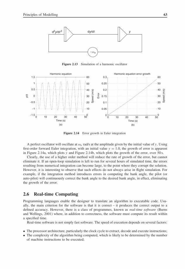
Principles of Modelling 63
−wn
ydy/dtd2y/dt 2
Figure 2.13 Simulation of a harmonic oscillator
0Time (s)
Harmonic equation Harmonic equation error growth
(a)
0
10
20
30
40
50
60
−1.5
−1
−0.5
0y(t)
Spe
ed (
m/s
)0.5
1
1.5
10 20 30 40 50 0Time (s)
(b)
0
10
20
30
40
50
60
0
0.05
0.1
0.15E
rror
Spe
ed (
m/s
)0.2
0.25
0.3
10 20 30 40 50
Figure 2.14 Error growth in Euler integration
A perfect oscillator will oscillate at ωn rad/s at the amplitude given by the initial value of y . Usingfirst-order forward Euler integration, with an initial value y = 1.0, the growth of error is apparentin Figure 2.14a, which plots y and Figure 2.14b, which plots the growth of the error, over 50 s.
Clearly, the use of a higher order method will reduce the rate of growth of the error, but cannoteliminate it. If an open-loop simulation is left to run for several hours of simulated time, the errorsresulting from numerical integration can become large, to the point where they corrupt the solution.However, it is interesting to observe that such effects do not always arise in flight simulation. Forexample, if the integration method introduces errors in computing the bank angle, the pilot (orauto-pilot) will continuously correct the bank angle to the desired bank angle, in effect, eliminatingthe growth of the error.
2.6 Real-time ComputingProgramming languages enable the designer to translate an algorithm to executable code. Usu-ally, the main criterion for the software is that it is correct – it produces the correct output to adefined accuracy. However, there is a class of programmes, known as real-time software (Burnsand Wellings, 2001) where, in addition to correctness, the software must compute its result withina specified time.
Real-time software is not simply fast software. The speed of execution depends on several factors:
• The processor architecture, particularly the clock cycle to extract, decode and execute instructions;• The complexity of the algorithm being computed, which is likely to be determined by the number
of machine instructions to be executed;

64 Principles of Flight Simulation
• The efficiency of the compilation process to translate a high-level description to machine instruc-tions;
• Any delays in acquiring inputs to the algorithm, or transmitting outputs, particularly data whichis read or written via a hardware interface.
For example, in an industrial process, bottles may be filled as they pass along a conveyor belt.The system depositing liquid in each bottle has a fixed period to execute its task. If, for anyreason, the processing was delayed, a bottle may only be partially filled. Such a system would haveto meet a stringent real-time requirement for the software. During the design phase, any timingconstraints will be specified and the software will be thoroughly tested to ensure that it meets ittiming requirements, under all possible conditions.
The standard approach in real-time systems is to allocate a fixed period, often known as a frame,during which all the computations are executed. These frames are executed repeatedly so thatthe functions in an application are repeated periodically, at the frame rate. Invariably, the framerate is matched to the step length used in numerical integration. In effect, the system marches intime, frame-by-frame where the frame period is sufficiently small so that there are no perceiveddiscontinuities in the simulation and any errors introduced by the numerical methods are kept to aminimum.
Modern computers can execute several million instructions per second. However, data transfersinvolving hardware devices are implemented at much slower speeds. For example, a serial lineoperating at 9600 baud (9600 bits per second) takes approximately one millisecond to transferone byte of data. At the receiver, the data arrives every millisecond or so, but the receiver hasno knowledge as to when the data will actually arrive – in effect the transfer is asynchronous.When the data arrives, it can be transferred from the hardware registers of the interface card tomemory, taking only a few microseconds. One option is for the processor to poll a device until ithas received incoming data, or in the case of transmission, to check if the device is ready to transmitmore data. However, this method requires the processor to execute instructions waiting for data toarrive before copying the data. Clearly this approach is wasteful of the processing capability of theprocessor, if it simply waits for a slow device. It would be preferable for the processor to spendits millisecond on more useful computations. This situation is resolved by exploiting the interruptmechanism provided for most processors, which provides a fundamental part of a real-time system.
In an interrupt driven system, the processor can initiate a transfer with a device but continue withuseful computations, executing instructions rather than simply polling the device for completionof a transfer. When the device has data available, the device interrupts the processor. The currentstate of the processor (the machine registers) is saved in a reserved area (usually a stack) andthe processor transfers control to an interrupt service routine allocated to service the interruptingdevice. In the interrupt service routine, the status of the device is checked, data is copied from thedevice registers to memory (typically a buffer) and the device may be set for another data transfer.Finally, the processor will return from the interrupt by re-instating the processor state at the time ofthe interrupt; this is achieved by reloading the machine registers from the region where they werepreserved at the time of the interrupt. The processor then resumes the instructions it was executingprior to the interrupt. The important point about this use of interrupts, which are microcoded inthe processor architecture, is that the processor does not waste any time waiting for relatively slowdevices and the overhead of managing input and output devices is negligible.
A modern operating system allows several processes to execute concurrently. In fact, the pro-cessor is switching between processes at relatively high rates in order to achieve this concurrency.The selection of the next process to run is made by a scheduler, which characterizes the operatingsystem. In a real-time operating system, the processes are usually allocated a priority and the sched-uler will select the highest priority process that is able to run. Clearly, a process that is waiting for
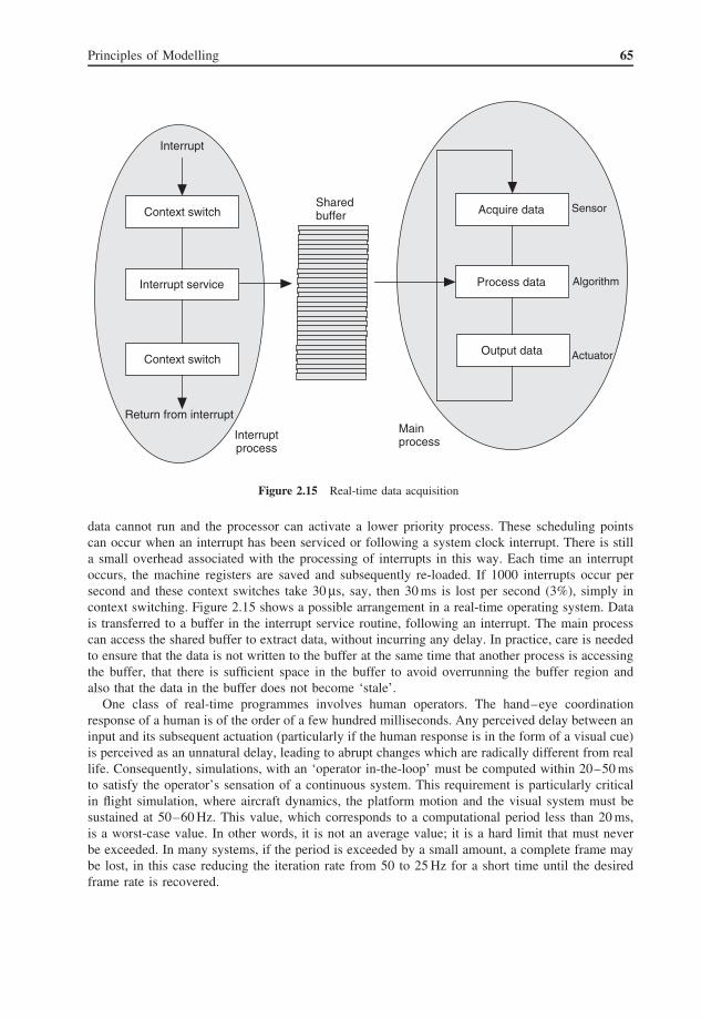
Principles of Modelling 65
Acquire data
Process data
Output data
Sensor
Algorithm
Actuator
Context switch
Interrupt service
Context switch
Interrupt
Return from interrupt
Sharedbuffer
Interruptprocess
Mainprocess
Figure 2.15 Real-time data acquisition
data cannot run and the processor can activate a lower priority process. These scheduling pointscan occur when an interrupt has been serviced or following a system clock interrupt. There is stilla small overhead associated with the processing of interrupts in this way. Each time an interruptoccurs, the machine registers are saved and subsequently re-loaded. If 1000 interrupts occur persecond and these context switches take 30 µs, say, then 30 ms is lost per second (3%), simply incontext switching. Figure 2.15 shows a possible arrangement in a real-time operating system. Datais transferred to a buffer in the interrupt service routine, following an interrupt. The main processcan access the shared buffer to extract data, without incurring any delay. In practice, care is neededto ensure that the data is not written to the buffer at the same time that another process is accessingthe buffer, that there is sufficient space in the buffer to avoid overrunning the buffer region andalso that the data in the buffer does not become ‘stale’.
One class of real-time programmes involves human operators. The hand–eye coordinationresponse of a human is of the order of a few hundred milliseconds. Any perceived delay between aninput and its subsequent actuation (particularly if the human response is in the form of a visual cue)is perceived as an unnatural delay, leading to abrupt changes which are radically different from reallife. Consequently, simulations, with an ‘operator in-the-loop’ must be computed within 20–50 msto satisfy the operator’s sensation of a continuous system. This requirement is particularly criticalin flight simulation, where aircraft dynamics, the platform motion and the visual system must besustained at 50–60 Hz. This value, which corresponds to a computational period less than 20 ms,is a worst-case value. In other words, it is not an average value; it is a hard limit that must neverbe exceeded. In many systems, if the period is exceeded by a small amount, a complete frame maybe lost, in this case reducing the iteration rate from 50 to 25 Hz for a short time until the desiredframe rate is recovered.

66 Principles of Flight Simulation
In many real-time systems, the application software runs under an operating system. This hasthe advantage that a consistent interface is provided for the system functions and the designerdoes not have to implement these functions in the application software. However, if the operatingsystem functions are used in combination with the application software, they must not extend thecomputation time by exceeding the frame limit. Any call to the operating system adds an explicitdelay to the application software. In practice, these calls are avoided in the time critical parts of theapplication software. But there are also aspects of operating system behaviour where computationsare executed by the operating system, independent of the application software. For example, theprocessing of an interrupt, the subsequent buffering of data and any context switching betweenprocesses amounts to an overhead imposed on application software. The only solution is to providea real-time system, where the application software can exert some influence on the behaviour,ordering and prioritization of operating system tasks.
For example, if a simulator has 32 analogue input channels and each analogue input requires100 µs for the analogue conversion to interrupt the computer and be copied to an application buffer,then 3.2 ms is lost every frame to the overhead of responding to interrupts, accessing the convertedvalue and copying it to memory. In a 20 ms frame, this amounts to approximately 15% of each framededicated to operating system functions rather than user applications. In practice, real-time operatingsystems are designed to minimize this overhead; some architectures are particularly efficient in termsof handling interrupts and input–output interfaces can reduce additional loading on the processor.Nevertheless, these effects and any other delays imposed by an operating system, need to beincluded in the real-time performance analysis of a simulation.
One further cause of delay occurs in the application software. In some algorithms, the numberof iterations depends on data values computed at run-time. For example, a series expansion mayterminate after five terms or six terms depending upon a simulation variable. Consequently, theremay be a wide variation in the frame time. Another example occurs in flight simulation, where anaerodynamic model is used while the aircraft is airborne whereas a mechanical dynamics model isused while the aircraft is taxiing on the runway. If there is a transition between these models, theremay be a jump in processing time during landing. If fact, both models might be executed in thetransitory phase during touch down when one or more of the wheels is in contact with the ground,where both the flight model and the undercarriage software are active.
In this latter case, the addition of execution times for each function must still not exceed the framelimit. In practice, although a real-time flight simulator may use a 20 ms frame, say, a conservativemargin is normally allocated to ensure that no one frame exceeds the frame limit, for example, toreduce the computation time to 15 ms. Such constraints require very detailed and extensive timinganalysis to ensure that no frame exceeds the fixed frame period for all the possible states andconstraints of the simulated system. Figure 2.16 shows a typical frame loading for a real-time flightsimulator. Although the 20 ms frame is never exceeded, the margin is only 3.5 ms, based on analysisof 1000 frames (50 s).
In the case where the frame period is exceeded, the designer has very limited choices:
• To increase the processor performance;• To simplify the complexity of the model;• To attempt to optimize the software.
Generally, it is not feasible in real-time simulation to allow processes to exceed the frame periodfor a few frames, in the hope that the simulation will catch up within a few frames, when lessprocessing is used (although such techniques are used in computer games). Nevertheless, framesare closely monitored in most real-time simulators, to monitor processor loading and to providemaintenance engineers with valuable diagnostics in the event of unexpected overload.
Principles of Modelling 67
01200
Fra
me
time
(ms)
1300
1400
1500
1600
1700
1800
200 400
Frames
600 800 1000
Figure 2.16 Frame activity
2.7 Data AcquisitionIn a flight simulator, there are numerous levers, knobs, switches and selectors which enable theflight crew to operate the simulator in the same way that they operate an aircraft. The position andstate of these inputs are measured as analogue or digital inputs, typically as a voltage, and are readinto a computer via a hardware interface. Similarly, there are many outputs in a simulator, whichdrive actuators, lamps, stick shakers and possibly flight instruments, where the simulator computerwrites the output signal to the hardware interface of the equipment.
Data is transferred to or from simulator equipment via input/output (I/O) cards, which provideboth digital and analogue signals. Such cards usually provide fixed voltage ranges and additionalsignal conditioning is provided to interface the equipment to I/O cards. Although variables arestored in memory as floating point numbers, typically with a resolution of 32 or 64 bits, I/O data istransferred as integer values, typically with a resolution of 10–16 bits and converted to a floatingpoint value for use in the flight model. However, it is important to appreciate that the resolutionof the acquired data is several orders of magnitude less than the program variables.
2.7.1 Data Transmission
For digital outputs, most I/O cards are only able to drive a few milliamps, usually at transistor-transistor logic (TTL) voltage levels (0–5 V). Simple amplifier circuits provide the necessary currentoutput and appropriate voltage range. They also usually provide circuit protection to protect theI/O card from inadvertent ‘shorting’ at the equipment.

68 Principles of Flight Simulation
Analogue output is more complicated. For digital to analogue (D/A) conversion, an I/O card willprovide a specific voltage range (or a set of fixed ranges) and a given resolution. For example, a12-bit 5-V D/A may provide 0 V for the digital value 000000000000 and 5 V for the digital (binary)value 111111111111, with a resolution of 1.22 mV. From the user’s perspective, the 12-bit D/Aoutput 0–5 V would correspond to unsigned integer values in the range 0–4095. Clearly, the scalingbetween a variable in an application and the D/A value is the responsibility of the programmer. Theleast significant bit of this D/A is 0.00122 V. Each bit is, in effect, a binary weighting, doublingat each stage from the least significant bit to the most significant bit, so that a 12-bit word withonly the most significant bit set corresponds to 2.5 V. For D/A, resistors can be arranged so thatthey contribute a binary-weighted value, with the voltages of each stage being added, as shown inFigure 2.17, for a 10-bit D/A. The resistor chain comprises binary-weighted resistors. The switchesS0 to S9 either ground the D/A input or provide a current Vref/R via each resistor R0 to R9, whichis summed by the operational amplifier.
The output is valid as soon as the inputs have settled and the conversion time depends only onthe slew rate of the operational amplifier and the switching time of the switches, providing veryfast digital to analogue conversion (of the order a few hundred nanoseconds). Although a circuitof this form is easy to construct, the resistance of each stage must have an accuracy (or tolerance)equal to the least significant bit. In practice, it would be very difficult to calibrate the circuit tomeet 0.1% accuracy (needed for a 10-bit D/A) for all resistors. The overall accuracy depends on theaccuracy of the reference voltage, the tolerance of the resistors and the impedance of the switches(which can usually be neglected).
For high-resolution D/As, this simple circuit cannot provide sufficient accuracy and an alternativecircuit, known as the R-2R ladder network is used, consisting only of resistor values R and 2R, asshown in Figure 2.18. The equivalent circuit is shown in Figure 2.19.
In this circuit, each voltage source is applied to two resistors 2R and R, giving a resistanceof 3R and therefore a current of V /3R, so that i1 = i2 = i3 = i4 in all loops. The current i4 isdivided equally on either side of node n4, so that node 4 supplies i4/2 to node 3, i4/4 to node 2and i4/8 to node 1 and so on. The total current in RL is (for this simple four-stage circuit) given
+
−
Vref
R9 R8 R7 R6 R0
Rf
Vout
S9 S8 S7 S6 S0
Inputs
0 V
Figure 2.17 Ten-bit digital to analogue conversion
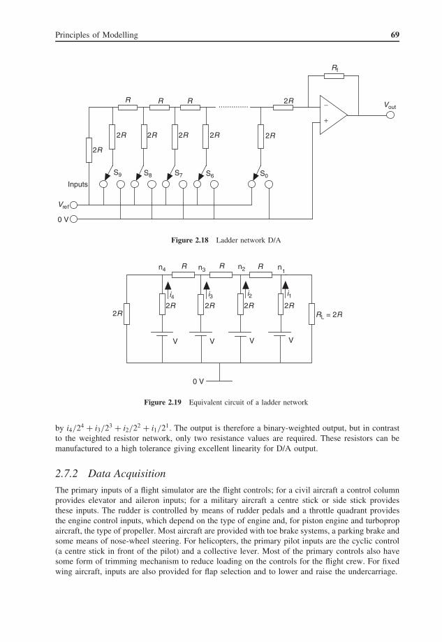
Principles of Modelling 69
..............
+
−
Vref
2R 2R 2R 2R 2R
Rf
Vout
S9 S8 S7 S6 S0
2R
R R R 2R
Inputs
0 V
Figure 2.18 Ladder network D/A
2R
V
R
2R
n4
i42R
i3
V V
R
2R
n2
i22R
i1
V
n3 n1
R
RL = 2R
0 V
Figure 2.19 Equivalent circuit of a ladder network
by i4/24 + i3/23 + i2/22 + i1/21. The output is therefore a binary-weighted output, but in contrastto the weighted resistor network, only two resistance values are required. These resistors can bemanufactured to a high tolerance giving excellent linearity for D/A output.
2.7.2 Data Acquisition
The primary inputs of a flight simulator are the flight controls; for a civil aircraft a control columnprovides elevator and aileron inputs; for a military aircraft a centre stick or side stick providesthese inputs. The rudder is controlled by means of rudder pedals and a throttle quadrant providesthe engine control inputs, which depend on the type of engine and, for piston engine and turbopropaircraft, the type of propeller. Most aircraft are provided with toe brake systems, a parking brake andsome means of nose-wheel steering. For helicopters, the primary pilot inputs are the cyclic control(a centre stick in front of the pilot) and a collective lever. Most of the primary controls also havesome form of trimming mechanism to reduce loading on the controls for the flight crew. For fixedwing aircraft, inputs are also provided for flap selection and to lower and raise the undercarriage.
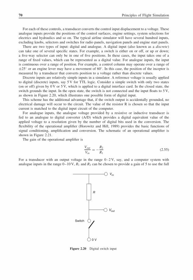
70 Principles of Flight Simulation
For each of these controls, a transducer converts the control input displacement to a voltage. Theseanalogue inputs provide the positions of the control surfaces, engine settings, system selections forelectrics and hydraulics and so on. The typical airline simulator will have several hundred inputs,excluding knobs, selectors and switches for radio panels, navigation panels and engine start panels.
There are two types of input: digital and analogue. A digital input (also known as a discrete)can take one of several specific states. For example, a switch is either on or off, or up or down;a five-way selector can only be in one of five positions. In these cases, the input takes one of arange of fixed values, which can be represented as a digital value. For analogue inputs, the inputis continuous over a range of position. For example, a control column may operate over a range of±25◦ or an engine lever may have a movement of 60◦. In this case, the position of the inceptor ismeasured by a transducer that converts position to a voltage rather than discrete values.
Discrete inputs are relatively simple inputs in a simulator. A reference voltage is usually appliedto digital (discrete) inputs, say 5 V for TTL logic. Consider a simple switch with only two states(on or off) given by 0 V or 5 V, which is applied to a digital interface card. In the closed state, theswitch grounds the input. In the open state, the switch is not connected and the input floats to 5 V,as shown in Figure 2.20, which illustrates one possible form of digital input.
This scheme has the additional advantage that, if the switch output is accidentally grounded, noelectrical damage will occur to the circuit. The value of the resistor R is chosen so that the inputcurrent is matched to the digital input circuit of the computer.
For analogue inputs, the analogue voltage provided by a resistive or inductive transducer isfed to an analogue to digital converter (A/D) which provides a digital equivalent value of theapplied voltage to a resolution given by the number of digital bits used in the conversion. Theflexibility of the operational amplifier (Horowitz and Hill, 1989) provides the basic functions ofsignal conditioning, amplification and conversion. The schematic of an operational amplifier isshown in Figure 2.21.
The gain of the operational amplifier is
Vout
Vin= −R2
R1(2.55)
For a transducer with an output voltage in the range 0–2 V, say, and a computer system withanalogue inputs in the range 0–10 V, R1 and R2 can be chosen to provide a gain of 5 to use the full
Vcc
R
0 V
Switch
Vout
Figure 2.20 Digital switch input

Principles of Modelling 71
−
+
Vin R1
R2
Vout
0 V
Figure 2.21 An operational amplifier
vin
vout
R3
R4
R1
R2
+−
R5
R6
+V
−V
0 V
Figure 2.22 Bias compensation for an operational amplifier
resolution of the analogue to digital conversion interface. Similarly if a bias is required to shift aninput in the range 2–3 V, it is not sufficient to simply modify the gain, it is also necessary to adjustthe bias of the input signal. The bias changes the signal to the range 0–1 V and a gain of 10 ensuresthe signal is in the range 0–10 V. A typical bias compensation circuit is shown in Figure 2.22.
The variable resistor R3, in conjunction with the resistor values R4, R5 and R6, can be used witha calibration voltage to provide sufficient bias to shift the input voltage to an appropriate range forthe A/D, combined with the gain selection afforded by resistors R1 and R2. Such compensation iscommonplace in a flight simulator. For example, movement may be sensed by a circular poten-tiometer. If the mechanical linkage is such that the wiper arm only traverses a proportion of thepotentiometer, the input can still be measured over the full operating range of an A/D to ensurethat no resolution is lost.
The A/D devices that have been developed for real-time applications are designed to meet thefollowing requirements:
• Speed of conversion – depending on the method of conversion, the analogue input is sampledand held during the conversion, which may take from a few nanoseconds to several milliseconds;
• Sampling rate – although this value depends on the conversion speed, the sampling speed mustmeet the iteration (or sampling) rate of a simulation. For example, if 32 analogue channels aresampled at 100 Hz, the actual sampling rate of the A/D is 3200 samples per second, approximately3 ms per sample;
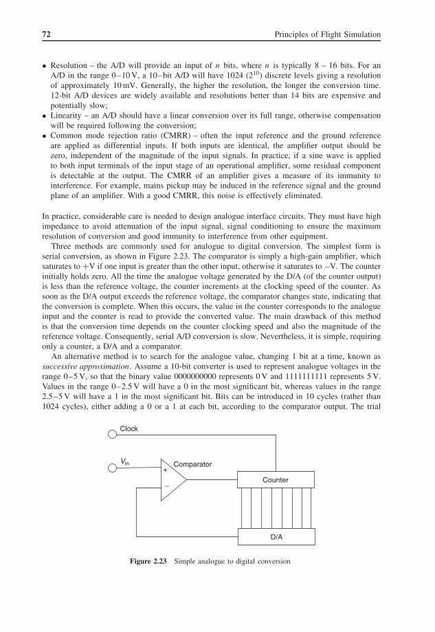
72 Principles of Flight Simulation
• Resolution – the A/D will provide an input of n bits, where n is typically 8 – 16 bits. For anA/D in the range 0–10 V, a 10–bit A/D will have 1024 (210) discrete levels giving a resolutionof approximately 10 mV. Generally, the higher the resolution, the longer the conversion time.12-bit A/D devices are widely available and resolutions better than 14 bits are expensive andpotentially slow;
• Linearity – an A/D should have a linear conversion over its full range, otherwise compensationwill be required following the conversion;
• Common mode rejection ratio (CMRR) – often the input reference and the ground referenceare applied as differential inputs. If both inputs are identical, the amplifier output should bezero, independent of the magnitude of the input signals. In practice, if a sine wave is appliedto both input terminals of the input stage of an operational amplifier, some residual componentis detectable at the output. The CMRR of an amplifier gives a measure of its immunity tointerference. For example, mains pickup may be induced in the reference signal and the groundplane of an amplifier. With a good CMRR, this noise is effectively eliminated.
In practice, considerable care is needed to design analogue interface circuits. They must have highimpedance to avoid attenuation of the input signal, signal conditioning to ensure the maximumresolution of conversion and good immunity to interference from other equipment.
Three methods are commonly used for analogue to digital conversion. The simplest form isserial conversion, as shown in Figure 2.23. The comparator is simply a high-gain amplifier, whichsaturates to +V if one input is greater than the other input, otherwise it saturates to –V. The counterinitially holds zero. All the time the analogue voltage generated by the D/A (of the counter output)is less than the reference voltage, the counter increments at the clocking speed of the counter. Assoon as the D/A output exceeds the reference voltage, the comparator changes state, indicating thatthe conversion is complete. When this occurs, the value in the counter corresponds to the analogueinput and the counter is read to provide the converted value. The main drawback of this methodis that the conversion time depends on the counter clocking speed and also the magnitude of thereference voltage. Consequently, serial A/D conversion is slow. Nevertheless, it is simple, requiringonly a counter, a D/A and a comparator.
An alternative method is to search for the analogue value, changing 1 bit at a time, known assuccessive approximation . Assume a 10-bit converter is used to represent analogue voltages in therange 0–5 V, so that the binary value 0000000000 represents 0 V and 1111111111 represents 5 V.Values in the range 0–2.5 V will have a 0 in the most significant bit, whereas values in the range2.5–5 V will have a 1 in the most significant bit. Bits can be introduced in 10 cycles (rather than1024 cycles), either adding a 0 or a 1 at each bit, according to the comparator output. The trial
Counter
D/A
−
+Comparator
Clock
Vin
Figure 2.23 Simple analogue to digital conversion
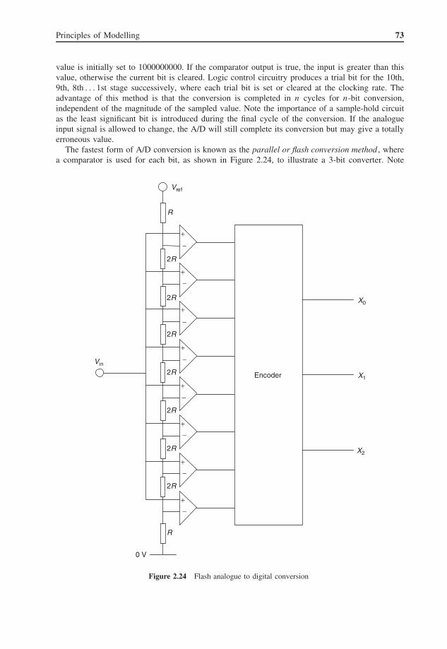
Principles of Modelling 73
value is initially set to 1000000000. If the comparator output is true, the input is greater than thisvalue, otherwise the current bit is cleared. Logic control circuitry produces a trial bit for the 10th,9th, 8th . . . 1st stage successively, where each trial bit is set or cleared at the clocking rate. Theadvantage of this method is that the conversion is completed in n cycles for n-bit conversion,independent of the magnitude of the sampled value. Note the importance of a sample-hold circuitas the least significant bit is introduced during the final cycle of the conversion. If the analogueinput signal is allowed to change, the A/D will still complete its conversion but may give a totallyerroneous value.
The fastest form of A/D conversion is known as the parallel or flash conversion method , wherea comparator is used for each bit, as shown in Figure 2.24, to illustrate a 3-bit converter. Note
Vin
Vref
Encoder
X0
X1
X2
R
2R
2R
2R
2R
2R
2R
2R
R
+−
+−
+
−
+−
+−
+−
+−
+−
0 V
Figure 2.24 Flash analogue to digital conversion

74 Principles of Flight Simulation
than 2n comparators are required for an n-bit converter. The resistor chain corresponds to 15/16,13/16, 11/16, 9/16, 7/16, 5/16, 3/16 and 1/16 of Vref, respectively. The voltage entered into theencoder is a binary-weighted value representing the sampled value. An encoder converts 2n bitsto its corresponding n bits. Note that this method requires 4096 comparators for 12-bit A/D andvery accurate resistors but the conversion rate is reduced to the settling time of the compara-tors. Consequently, flash A/D is used in very high performance signal acquisition applications. Insimulation, a sampling rate of 50 Hz for 32 channels requires an overall A/D conversion speed of640 Hz, approximately 1500 µs per sample, which is well within the conversion time of a successiveapproximation method.
Considerable attention is given to digital and analogue I/O in flight simulators. The devicesselected must provide linearity, sufficient resolution and fast conversion times. Problems can occuras a result of poor grounding of analogue signals; to avoid this, differential analogue inputs are usedwhere the ground reference and signal are provided for each connection. Care is also needed to avoidinterference, although generally this results from mains interference or induced noise from electricalmachinery. Cross-talk, resulting in interference between wires is rare; as the signal frequenciesin flight simulation applications are sufficiently low, this form of interference is unlikely to beencountered. Some I/O devices provide autonomous data transfers, requiring only initialization; thetransfers are then implemented independent of the processor. Alternatively, with low-cost embeddedsystems, it is straightforward to provide dedicated I/O systems, with I/O data transferred to thesimulator computers via a network.
2.8 Flight DataIn flight simulation, much of the data is provided in the form of graphical or tabular data. Sometimes,this is because it is the most convenient or efficient form to represent, store and organize thedata. Alternatively, the data may be non-linear or functions of several variables and a graphicalformat simplifies the method to communicate the data. Data may be acquired at regular points oralternatively, for a limited set of points where it was convenient (or safe) to record the values.However, during simulation, it is necessary to compute values which will probably not correspondwith the acquired data and it is necessary to interpolate between data points or extrapolate from aset of data points. Clearly, the processes of interpolation and extrapolation can introduce errors inthe computation of numeric values and care has to be given to ensure that errors generated in theseprocesses do not affect the solution of the equations or the behaviour of the simulated system.
Often data will be provided as a set of data points. For example, the values in Table 2.5 wererecorded for a component of the dCL/dα lift curve for a fighter aircraft in the subsonic range (belowMach 1). The resultant graph from these 12 points is shown in Figure 2.25.
Data represented in this form has three advantages:
• It is compact – the function is represented as 12 coordinate pairs;• Interpolation between individual points is straightforward;• The function passes through the specific tabulated points.
However, this data also exhibits several disadvantages:
• It is necessary to search for a specific line segment as a function of M in order to find the endpoints of a segment;
• At each tabulated point there is a discontinuity in the function which is probably not representativeof the actual system and may introduce dynamics (resulting from an abrupt change) which isinappropriate.
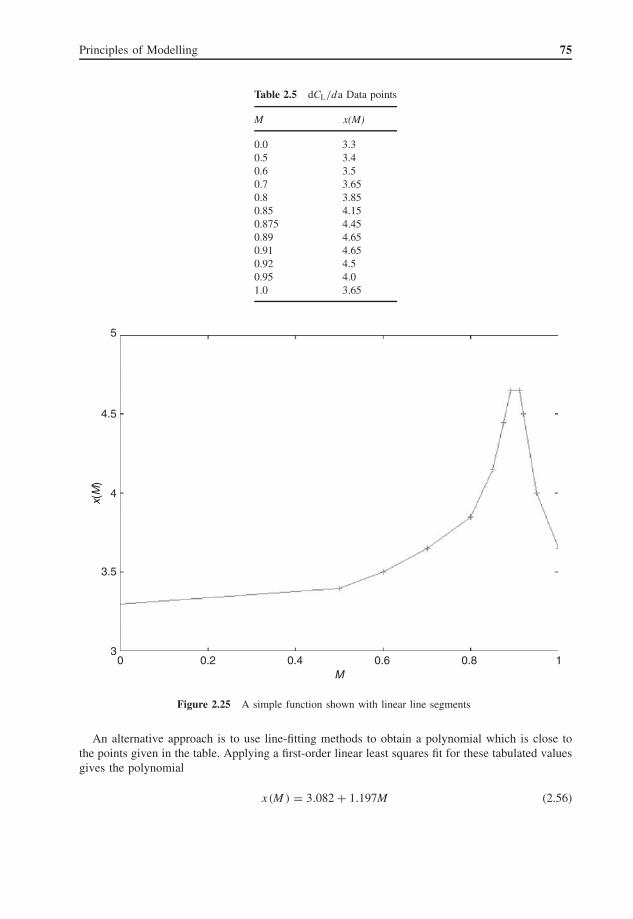
Principles of Modelling 75
Table 2.5 dCL/da Data points
M x(M)
0.0 3.30.5 3.40.6 3.50.7 3.650.8 3.850.85 4.150.875 4.450.89 4.650.91 4.650.92 4.50.95 4.01.0 3.65
03
3.5
4
4.5
5
0.2
x(M
)
0.4M
0.6 0.8 1
Figure 2.25 A simple function shown with linear line segments
An alternative approach is to use line-fitting methods to obtain a polynomial which is close tothe points given in the table. Applying a first-order linear least squares fit for these tabulated valuesgives the polynomial
x(M ) = 3.082 + 1.197M (2.56)

76 Principles of Flight Simulation
A second-order linear least squares fit for the same data gives the polynomial
x(M ) = 3.175 + 0.505M + 0.672M 2 (2.57)
Both polynomial approximations are shown in Figure 2.26; it is clear that the polynomials neitherresemble the data characteristics nor pass through any of the actual data points.
Another approach is to compute a high-order polynomial. However, a least squares fit usinga 12th-order polynomial is still unlikely to match the data closely and a polynomial fit devisedto pass through all the data points (e.g. a Chebyshev polynomial) is likely to contain oscillatorycharacteristics that are not evident in the data.
Bearing in mind that data acquired experimentally (e.g. from flight trials) is probably valid atthe acquired data points (within the resolution of the sensor measurement) and moreover, that anexperimentalist capturing the data may have knowledge of the system to justify taking extra pointsin specific ranges or omitting data points where the characteristic is predictable, then a smooth linepassing through all the points with no apparent discontinuity is potentially a better approximation.This approach is similar to the plastic ‘flexicurves’ that were widely used by draughtsmen andengineers for curve fitting in the days when graphs were plotted on paper rather than computerscreens.
The most commonly used curve fitting method to provide a smooth continuous curve passingthrough all data points is spline fitting. The examples to generate lookup tables from flight dataused in this book are based on the spline fitting algorithms in Press et al., (2007). Figure 2.27 showsa spline fit to the data in Figure 2.25 generating 100 points for the range 0–1.0, which shows thatthe curve is smooth and continuous while also passing through all the data points.
03
3.5
4
4.5
5Data file
Data3.082 + 1.197∗x3.175 + 0.505∗x+0.672∗x∗x
0.2
x(M
)
0.4 0.6
M
0.8 1
Figure 2.26 First and second-order linear least squares fit to the data points
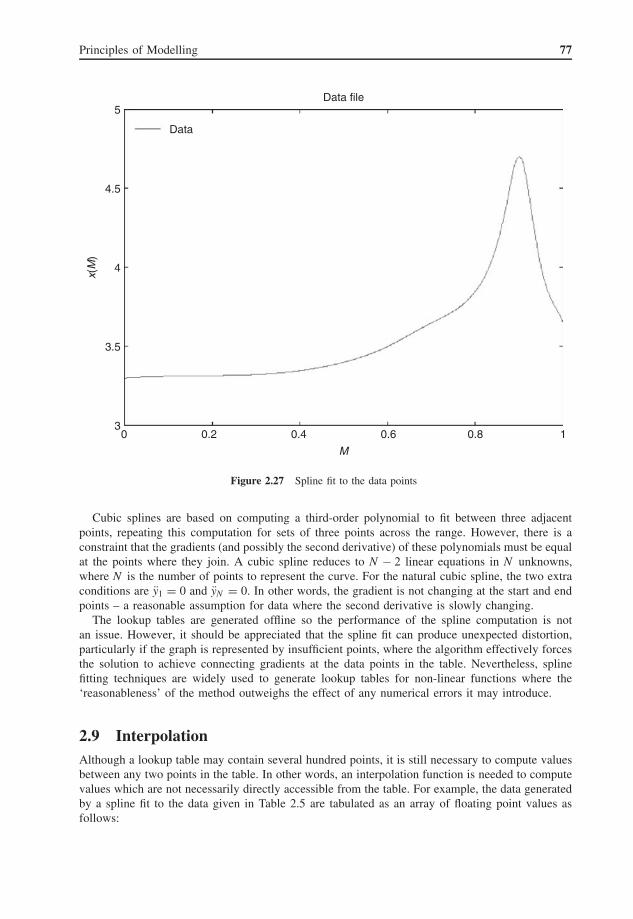
Principles of Modelling 77
03
3.5
4
4.5
5
Data
Data file
0.2
x(M
)
0.4
M
0.6 0.8 1
Figure 2.27 Spline fit to the data points
Cubic splines are based on computing a third-order polynomial to fit between three adjacentpoints, repeating this computation for sets of three points across the range. However, there is aconstraint that the gradients (and possibly the second derivative) of these polynomials must be equalat the points where they join. A cubic spline reduces to N − 2 linear equations in N unknowns,where N is the number of points to represent the curve. For the natural cubic spline, the two extraconditions are y1 = 0 and yN = 0. In other words, the gradient is not changing at the start and endpoints – a reasonable assumption for data where the second derivative is slowly changing.
The lookup tables are generated offline so the performance of the spline computation is notan issue. However, it should be appreciated that the spline fit can produce unexpected distortion,particularly if the graph is represented by insufficient points, where the algorithm effectively forcesthe solution to achieve connecting gradients at the data points in the table. Nevertheless, splinefitting techniques are widely used to generate lookup tables for non-linear functions where the‘reasonableness’ of the method outweighs the effect of any numerical errors it may introduce.
2.9 InterpolationAlthough a lookup table may contain several hundred points, it is still necessary to compute valuesbetween any two points in the table. In other words, an interpolation function is needed to computevalues which are not necessarily directly accessible from the table. For example, the data generatedby a spline fit to the data given in Table 2.5 are tabulated as an array of floating point values asfollows:

78 Principles of Flight Simulation
float f1tab[] = {
3.3000, 3.3019, 3.3036, 3.3051, 3.3065, 3.3076, 3.3087, 3.3096, 3.3104, 3.3111,
3.3116, 3.3121, 3.3126, 3.3129, 3.3132, 3.3135, 3.3138, 3.3141, 3.3143, 3.3146,
3.3149, 3.3153, 3.3157, 3.3161, 3.3167, 3.3173, 3.3181, 3.3189, 3.3199, 3.3211,
3.3224, 3.3238, 3.3255, 3.3273, 3.3293, 3.3316, 3.3341, 3.3368, 3.3398, 3.3430,
3.3465, 3.3504, 3.3545, 3.3589, 3.3637, 3.3688, 3.3743, 3.3801, 3.3864, 3.3930,
3.4000, 3.4074, 3.4153, 3.4237, 3.4327, 3.4422, 3.4524, 3.4632, 3.4747, 3.4870,
3.5000, 3.5138, 3.5284, 3.5434, 3.5588, 3.5744, 3.5900, 3.6056, 3.6208, 3.6357,
3.6500, 3.6637, 3.6772, 3.6912, 3.7062, 3.7228, 3.7416, 3.7631, 3.7880, 3.8167,
3.8500, 3.8887, 3.9353, 3.9925, 4.0631, 4.1500, 4.2554, 4.3802, 4.5233, 4.6500,
4.7010, 4.6500, 4.5000, 4.3211, 4.1476, 4.0000, 3.8930, 3.8184, 3.7622, 3.7107,
3.650};
The table contains 100 values in the range 0–1.0, giving an interval of 0.01. Clearly, it is assumedthat values outside this range will not be required, although it would be prudent to either detect suchoccurrences or to provide sensible default values in such a case. Alternatively, extrapolation methodscan be used to predict values outside the range from values in the table. For 2D interpolation, weneed to return the value f 1 (M ) for any value of M in the range 0–1.0.
A fragment of the curve is shown in Figure 2.28. From the trigonometry of similar triangles, intriangle ABC
p
q= r
�x(2.58)
x1 x2
(x,y)
(x1,y1)
(x2,y2)
A
B
C
p q
∆x
r
Figure 2.28 2D interpolation

Principles of Modelling 79
But p = y − y1, q = y2 − y1 and r = x − x1 which yields
y − y1
y2 − y1= x − x1
�xgiving
y = y1 + (x − x1)(y2 − y1)
�x(2.59)
�x is easily computed from the overall range and the number of values in the table. x1 is thenearest x value in the table below x , which allows the offset in the table to be computed to locatey1. y2 is the adjacent value above y1 in the table.
The C code procedure for 2D interpolation is shown in Example 2.3.
Example 2.3 2D interpolation
float tabval(float t[], float x, float xmin, float xmax, unsigned int size)
{
unsigned int p;
float dx;
float x1;
float y1, y2;
dx = (xmax - xmin) / (float) size;
p = (unsigned int) ((x - xmin) / dx);
if (p >= size) {
return t[size];
}
else {
x1 = xmin + (float) p * dx;
y1 = t[p];
y2 = t[p+1];
return y1 + (x - x1) * (y2 - y1) / dx;
}
}
For example, to access the value in f1tab for a mach number of 0.345, the following code couldbe executed:
v = tabval(f1tab, 0.345, 0.0, 1.0, 100);
The same concept can be readily extended to functions of two variables, where 3D interpolationis used to compute y = f (x , z ). Values of x over a specific range are stored as a set of values forspecific values of z , to represent the graph shown in Figure 2.29.
Consider the case for the computation of engine coefficient of thrust CT for a piston enginewhich is a function of the blade angle β and the advance ratio J . For each value of β, CT valuesare stored for values of J in the range 0–2.2 in steps of 0.2. Nine sets of data are stored for values

80 Principles of Flight Simulation
x
yz
Figure 2.29 3D interpolation
of β in the range 0–40◦ in steps of 5◦. A two-dimensional array representing these values is shownbelow.
float CtTable[] = {
/*
0.0 0.2 0.4 0.6 0.8 1.0
1.2 1.4 1.6 1.8 2.0 2.2 J */
0.000, 0.000, 0.000, 0.000, 0.000, 0.000,
0.000, 0.000, 0.000, 0.000, 0.000, 0.000, /* 0 */
0.000, 0.000, 0.000, 0.000, 0.000, 0.000,
0.000, 0.000, 0.000, 0.000, 0.000, 0.000, /* 5 */
0.000, 0.000, 0.000, 0.000, 0.000, 0.000,
0.000, 0.000, 0.000, 0.000, 0.000, 0.000, /* 10 */
0.092, 0.084, 0.065, 0.037, 0.007, -0.022,
-0.050, -0.080, -0.108, -0.137, -0.167, -0.196, /* 15 */
0.099, 0.096, 0.089, 0.064, 0.036, 0.006,
-0.023, -0.054, -0.084, -0.115, -0.144, -0.175, /* 20 */
0.118, 0.114, 0.110, 0.095, 0.071, 0.043,
0.013, -0.017, -0.045, -0.073, -0.102, -0.131, /* 25 */
0.115, 0.110, 0.106, 0.100, 0.101, 0.080,
0.053, 0.024, -0.007, -0.038, -0.068, -0.098, /* 30 */
0.139, 0.132, 0.126, 0.119, 0.113, 0.108,
0.089, 0.065, 0.038, 0.010, -0.020, -0.048, /* 35 */
0.141, 0.135, 0.128, 0.123, 0.120, 0.114,
0.112, 0.101, 0.080, 0.057, 0.030, 0.005}; /* 40 */
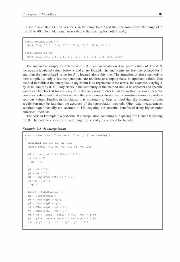
Principles of Modelling 81
Each row contains CT values for J in the range 0–2.2 and the nine rows cover the range of β
from 0 to 40◦. Two additional arrays define the spacing for both J and β.
float BetaSpacing[] =
{0.0, 5.0, 10.0, 15.0, 20.0, 25.0, 30.0, 35.0, 40.0};
float JSpacing[12] =
{0.0, 0.2, 0.4, 0.6, 0.8, 1.0, 1.2, 1.4, 1.6, 1.8, 2.0, 2.2};
The method is simply an extension of 2D linear interpolation. For given values of J and β,the nearest tabulated values below J and β are located. The end points are first interpolated for β
and then the interpolated value for J is located along this line. The attraction of these methods istheir simplicity; only a few computations are required to compute these interpolated values. Onemethod to validate the interpolation algorithm is to regenerate these terms, for example, varying Jby 0.001 and β by 0.001. Any errors in the continuity of the method should be apparent and specificvalues can be checked for accuracy. It is also necessary to check that the method is correct near theboundary values and that values outside the given ranges do not lead to run-time errors or producespurious values. Finally, in simulation it is important to bear in mind that the accuracy of dataacquisition may be less than the accuracy of the interpolation methods. Often data measurementsacquired experimentally are accurate to 1%, negating the potential benefits of using higher ordernumerical methods.
The code in Example 2.4 performs 3D interpolation, assuming 0.2 spacing for J and 5.0 spacingfor β. The code to check for a valid range for J and β is omitted for brevity.
Example 2.4 3D interpolation
static float Cval(float beta, float j, float CTable[])
{
unsigned int n1, p1, p2, q1;
float beta1, x1, y1, y2, y3, y4, y5, y6;
n1 = (unsigned int) (beta / 5.0);
if (n1 > 7) {
n1 = 7;
}
p1 = n1 * 12;
p2 = p1 + 12;
q1 = (unsigned int) (j / 0.2);
if (q1 > 10) {
q1 = 10;
}
beta1 = BetaSpacing[n1];
x1 = JSpacing[q1];
y1 = CTable[p1 + q1];
y2 = CTable[p2 + q1];
y4 = CTable[p1 + q1 + 1];
y5 = CTable[p2 + q1 + 1];
y3 = y1 + (beta - beta1) * (y2 - y1) / 5.0;
y6 = y4 + (beta - beta1) * (y5 - y4) / 5.0;
return y3 - (j - x1) * (y3 - y6) / 0.2;
}

82 Principles of Flight Simulation
2.10 Distributed SystemsFor airline flight simulators up to the 1980s, the computers were housed in a large air-conditionedcomputer room, with thick bundles of cables between the computers and the simulator. Withcomputing resources at a premium, each computer performed a dedicated set of functions, typicallywith one computer system for the flight model, another for the motion system and additional imagegenerators for the visual system.
Arguably, this was an early form of distributed computing. The flight model outputs to themotion platform and visual system were transmitted as analogue voltages. If the pitch range of±90◦ is given by ±10 V, a resolution of 1 mV corresponds to 0.009◦. If the vertical field of viewis 40◦ and corresponds to 1000 pixels, say, then each pixel subtends 0.04◦ vertically and smoothangular motion can be achieved. However, if position is passed in the same way, corresponding to±10 km, then 1 mV corresponds to 1 m, with the likelihood of ‘jerky’ motion near the runway.
However, if the information is transmitted digitally between computers, these problems canbe avoided, as values are transmitted as floating-point numbers between computers. Prior to theavailability of low-cost network interfaces, three options were available for inter-processor com-munication:
• Shared or reflective memory – a bank of memory is provided which can be accessed by two ormore computer systems; this memory is seen in the hardware memory space of each processorconnected to the shared memory. While this approach ensures high-speed data transfers, thedrawback of this system is the number of address and data lines needed to connect a processorto the shared memory and the need for logic to ensure atomic access to the shared memory toavoid data being read while it is changing;
• Parallel data lines between computers – 8 or 16 parallel data lines provide fast data rates but atthe expense of the cabling for data and control (handshake) lines;
• Serial data lines – although only two wires may be needed, the data rates are typically limitedto 19,200 bits per second over a distance of up to 20 m.
The third option seems attractive; RS-232 and RS-422 serial interfaces are widely available.However, 19,200 bits per second is approximately 2000 bytes per second. At 50 frames persecond, with 4 bytes per variable, this transfer speed corresponds to 10 variables per frame. Con-sequently, communications between computers require significantly high data rates for real-timesimulation.
Fortunately, as the cost of computers fell and processing speeds increased, serial network inter-faces were developed for local networking, particularly Ethernet. The benefits of these advancesare twofold: first, data rates of 10 Mbits per second are commonplace and secondly, simulatorfunctions can be programmed across an array of interconnected processors rather than allocated toa single high-speed processor.
Since the 1990s, most real-time simulators have exploited the distributed architecture affordedby low-cost networks and workstations. For the simulator designer, the software can be parti-tioned across an array of processors according to the structure of the simulator software and theperformance of the processors. Data is shared between processors by transmitting packets over adedicated local network. The software is programmed in a high-level language, each processor hasan operating system to support software functions and software libraries have been developed tosupport standard network data transfers.
In a local area network, integrity of the data transfers is paramount and the protocols providedfor a network achieve this by re-sending packets if errors are detected or if a packet transfer is notacknowledged within a short time. However, in a real-time system, delays resulting from retriedpacket transmissions would be unacceptable. All packet transfers must be completed during eachfixed frame and these transfers must be guaranteed to meet any timing constraints because, in a
Principles of Modelling 83
distributed system, a node depends on the other nodes to provide data that is timely and consistent.Any variation in the periodicity of the data transfers and the time taken to transfer data may affectthe real-time performance and violate the strict timing constraints imposed by a real-time system.
Data transfers in a real-time system must be deterministic. That is to say, the time betweensending the data from a node and it being taken by another node is known a priori – it is predictableand invariant. However, the action of generating a packet and simply transmitting it directly overthe network can lead to indeterministic transfers. The most common problem is that two nodestransmit simultaneously leading to a ‘collision’ of bus traffic. Typically, a collision is resolvedby nodes re-transmitting their packets at a later time. However, subsequent transfers may leadto further collisions, further increasing latency in transfers, violating the timing constraints of areal-time system.
To ensure deterministic transfers in a real-time network, all nodes must comply with a protocol,that is, the set of rules that are adhered to by all the nodes in the network. If the protocol isfollowed, only one node transmits at a time, avoiding collisions and guaranteeing that the delaysincurred in the transfer depend only on the bus characteristics.
Three forms of deterministic protocols are used in real-time networks:
• Master-slave transfers – one node is allocated as a master node. It sends a packet to a slavenode which is then allowed to transfer its packets. When these transfers are completed, the slavesends an acknowledgement packet to the master. The master then sends a packet to another nodeand the cycle repeats until all slave nodes have transmitted their packets. There is a significantoverhead in terms of the packet transfers to activate the slave node transfers and to acknowledgetheir completion, reducing the bandwidth available for data transfers between nodes;
• Token passing – a node only transmits data when it holds a token. On completion of transfersby a node, the token is passed (as a packet) to another node which then has exclusive accessto the bus. Each node has a list of the schedule of transfers, passing the token to the next nodein the schedule after completing its data transfers. The protocol assumes that all nodes respondimmediately (otherwise, delays in one node can accumulate for the other nodes) and depends onall nodes cooperating;
• Time division multiple access (TDMA) – within each frame, a unique time slot is allocated toeach node. A node can only transmit during its slot and the time taken for the transfers mustnot exceed the duration of the slot. Such schemes depend on accurate synchronization of thelocal clocks of the slave nodes. In practice, a margin has to be built in to ensure that nodes onlytransfer data within their slots, resulting in some loss of overall bandwidth.
There are many other forms of protocols used in real-time networks and many network archi-tectures have evolved to meet the wide range of demands in real-time computing. In real-timesimulation, the criterion is that the protocol is deterministic, reliable and has sufficient bandwidthto accommodate the number of variables transferred between the simulator computers each frame.
The Open Systems Interconnection (OSI) model has seven layers defining network protocolrequirements, as shown in Figure 2.30. Its use is widespread as it is followed by all networksystem designers and is used in the majority of networks throughout the world. The adherenceto this standard provides a very high degree of interoperability across platforms and portability ofsoftware. Layers 4–7 provide end-to-end file transfer across the world. By necessity, these protocolsrequire re-try mechanisms for loss or corruption of data, acknowledgement of received packets anddetection of unresponsive nodes. These protocols are machine independent and provide networkaddressing to transfer data between computers across continents. However, the complexity of theseprotocols and the flexibility they must provide restrict their use to non real-time applications. Inother words, these protocols are non-deterministic.
The lower levels 1–3 can provide deterministic protocols, while still affording the advantages ofnode addressing, standardization, interoperability and portability of application software. Level 1
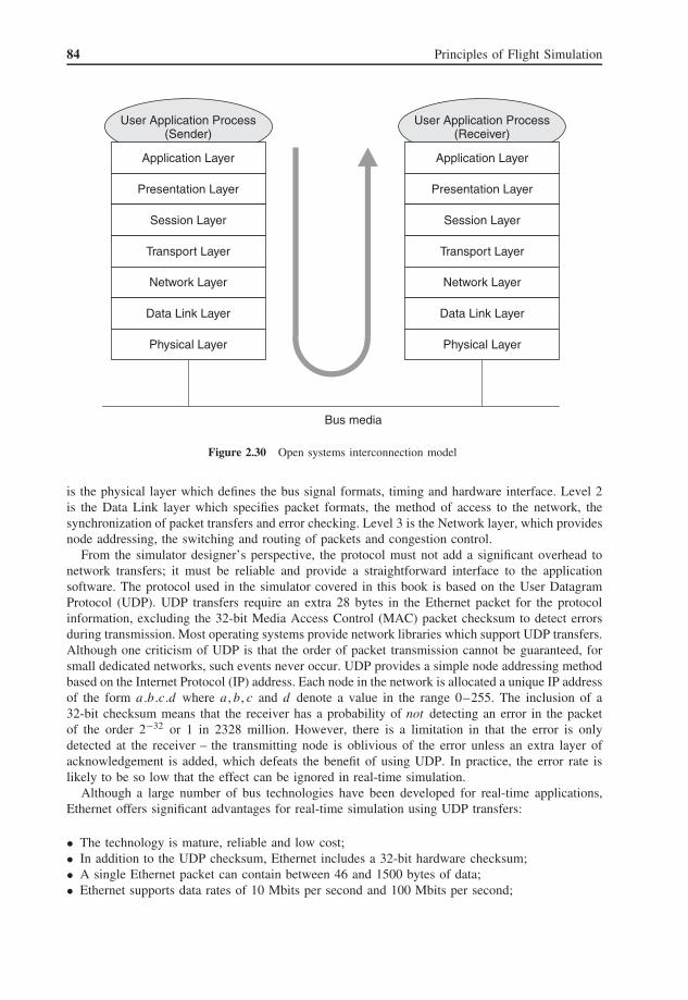
84 Principles of Flight Simulation
Bus media
User Application Process(Sender)
Application Layer
Presentation Layer
Session Layer
Transport Layer
Network Layer
Data Link Layer
Physical Layer
User Application Process (Receiver)
Application Layer
Presentation Layer
Session Layer
Transport Layer
Network Layer
Data Link Layer
Physical Layer
Figure 2.30 Open systems interconnection model
is the physical layer which defines the bus signal formats, timing and hardware interface. Level 2is the Data Link layer which specifies packet formats, the method of access to the network, thesynchronization of packet transfers and error checking. Level 3 is the Network layer, which providesnode addressing, the switching and routing of packets and congestion control.
From the simulator designer’s perspective, the protocol must not add a significant overhead tonetwork transfers; it must be reliable and provide a straightforward interface to the applicationsoftware. The protocol used in the simulator covered in this book is based on the User DatagramProtocol (UDP). UDP transfers require an extra 28 bytes in the Ethernet packet for the protocolinformation, excluding the 32-bit Media Access Control (MAC) packet checksum to detect errorsduring transmission. Most operating systems provide network libraries which support UDP transfers.Although one criticism of UDP is that the order of packet transmission cannot be guaranteed, forsmall dedicated networks, such events never occur. UDP provides a simple node addressing methodbased on the Internet Protocol (IP) address. Each node in the network is allocated a unique IP addressof the form a.b.c.d where a , b, c and d denote a value in the range 0–255. The inclusion of a32-bit checksum means that the receiver has a probability of not detecting an error in the packetof the order 2−32 or 1 in 2328 million. However, there is a limitation in that the error is onlydetected at the receiver – the transmitting node is oblivious of the error unless an extra layer ofacknowledgement is added, which defeats the benefit of using UDP. In practice, the error rate islikely to be so low that the effect can be ignored in real-time simulation.
Although a large number of bus technologies have been developed for real-time applications,Ethernet offers significant advantages for real-time simulation using UDP transfers:
• The technology is mature, reliable and low cost;• In addition to the UDP checksum, Ethernet includes a 32-bit hardware checksum;• A single Ethernet packet can contain between 46 and 1500 bytes of data;• Ethernet supports data rates of 10 Mbits per second and 100 Mbits per second;

Principles of Modelling 85
• Ethernet cards are compliant with the OSI model, providing a simple and consistent interfacefor applications.
At 10 Mbits per second, the data rate of bus transfers is of the order 1 MB per second or 5000floating point variables per frame (at 50 Hz). Even if only 10% of the frame is allocated to transfers,some 500 variables can be transferred between nodes each frame.
The disadvantage of Ethernet is that strictly it is not a deterministic medium. The hardware in anEthernet interface uses a Carrier Sense Multiple Access Collision Detection (CSMA/CD) protocol.The carrier used in data transmission is detected. If the bus is quiet then a node can attempt totransfer its packet (the multiple access term implies than any node can attempt to gain access to thebus at any time). In the case where two nodes transmit simultaneously (within one bit period), thisevent is detected by the hardware interface, the transmission is stopped and the interface waits fora short random time before it attempts to re-transmit its packet. The random delay applied by eachnode following a collision reduces the likelihood of the same collision re-occurring. The networkintegrity is based on these random re-try intervals and is therefore non-deterministic. In theory, twocolliding nodes could repeatedly select the same random delay indefinitely. In practice, this wouldnever occur. Nevertheless, any collision will lead to additional network transfers, adding latency tothe transfers so that deterministic data transfers cannot be assured for a real-time network. However,if the transfers are sequenced so that only one node ever transmits at any time, these transfers arecontention-free, no collisions will occur and the resultant data transfers will be deterministic.
Ethernet offers one further advantage that is attractive in real-time applications; multicast datatransfers are supported, allowing a data packet to be broadcast to all nodes on the network. In thecase where one node needs to transfer the same packet to five nodes, say, it can broadcast the packetand the five nodes needing the data can read the packet from the network. Other nodes, not needingthe data can discard the packet. In real-time simulation, multicast transfers can reduce significantlythe number of transfers per frame. For example, in a flight simulator, the aircraft pitch attitudeis used in the flight model equations, the motion platform dynamics, for the aircraft instrumentdisplays and also by the visual system.
For a dedicated real-time system, the use of IP addresses is important. The nodes on the networkare likely to be addressed in some logical manner in the simulator algorithms. There is a need tomap between the IP addresses allocated to the nodes on the network and the logical addresses usedin the simulation. However, if the simulator designer is able to allocate the IP addresses, these canbe given numeric values corresponding to the logical addresses. Most operating systems allow thenode IP addresses to be statically allocated. For example, in a system of five nodes, if the followingIP addresses are allocated: 192.168.1.1, 192.168.1.2, 192.168.1.3, 192.168.1.4 and 192.168.1.5, thenthese addresses can correspond to nodes 1–5. For this group of nodes, the broadcast address is192.168.1.255. A node can inspect the IP address of an incoming packet and effectively route thepacket to the appropriate software requiring the specific packet. Of course, this convention assumesa dedicated network, specific to a real-time application. If this network was connected to a localarea network, all incoming UDP packets would need to be checked and of course, contention forthe network would inhibit real-time access.
In fact, there is a protocol below the UDP known as the Media Access Control (MAC) layer.Each Ethernet card has a unique 6-byte physical address and the source and destination MACaddresses are included in the packet. However, this arrangement would require that any real-timeapplication software is dependent on specific hardware addresses and that the transfers would needto be implemented as ‘raw sockets’. Most operating systems prohibit raw socket transfers as theymake the computer system vulnerable to attacks. Consequently, UDP transfers are often used inreal-time applications:
• The bandwidth overhead is minimal, whereas protocols such as transmission control proto-col/internet protocol (TCP/IP) introduce significant latency for real-time applications;

86 Principles of Flight Simulation
• The interface between the application software and the operating system complies with a pub-lished standard and is straightforward;
• UDP transfers facilitate the implementation of deterministic protocols for real-time applications.
At the level of the operating system, data is formed as a packet in the memory of the computerand copied to the memory of another computer by the network controllers, as shown in Figure 2.31.
The application software forms the data in the packet in memory. The network interface isprogrammed to copy this data from memory to the databus, using direct memory access (DMA)independent of the processor. The encoding of the data from parallel to serial is managed by thenetwork controller. The interface can interrupt the processor to indicate completion of the transfers.Similarly at the receiver, the data is copied from the databus as serial data to memory using DMA.The location of the packet in memory and the form of the transfer is defined by programmingthe interface card. When the transfer is completed, the processor is interrupted to indicate thata new packet is available. In addition, the status of the transfer can also be accessed from theinterface.
From the user’s perspective, the operating system will perform many of these tasks, reducing thetask of reading and writing packets to the allocation of memory for the packet and the constructionof the data packet in memory, as shown in Figure 2.32, which outlines the division of responsibilitybetween the application process and the operating system.
In stage 1, the application writes the data to be transferred into the packet, which is allocatedin main memory. In stage 2, the operating system is requested to transfer the data. In stage 3, theoperating system will form the packet as a valid UDP, say, adding any protocol headers and achecksum. The network hardware interface is then accessed in stage 4 to initiate the transfer. Thecompletion of the transfer is likely to be signalled as an interrupt (stage 5) and the applicationsoftware can subsequently check the result of the transfer (stage 6). The point to stress is that theuser application simply forms a data packet, independent of any protocol, then issues a request tothe operating system to transfer the packet, but complying with a specific protocol and is able tomonitor the outcome of the transfer.
Processor
Memory
Packet
Parallel
Serial
Databus
Processor
Parallel
Serial
Memory
Packet
Networkinterface
Networkinterface
Signal
Figure 2.31 Packet transfers

Principles of Modelling 87
Memory
Packet
Userapplication
Type of transferSource node addressPacket address
Resultstatus
Formpacket
Operatingsystem
Accesspacket
Low-levelpacketdriver
Sendpacket
Interrupt
2
1
3
45
6
Figure 2.32 Operating system packet transfers
Programs 2.1 and 2.2 show the repeated transfers of UDP packets broadcast between two nodes,using the broadcast IP addresses 192.168.1.255. The network constants and functions are definedin the system-wide header files types.h, socket.h and netinet.h . Three functions are used to send apacket. The function socket opens a socket between the user application and the operating system.Packets are transferred in sendudp.c using the function sendto and on completion of the transfers,close is used to shut down the socket connection. The symmetry of the code used to read packetsin readudp.c is clear. A socket is opened and closed in the same way, but the function revcfrom isused to read packets. The status of these system calls is checked after each call – a negative valueindicates a problem. Note the simplicity of transferring data between nodes, which is accomplishedin some 70–80 lines of C code. Notice also that the structure and content of the data buffer is leftto the user to define, in this example it is simply an array of 200 integers. In sendpkt.c, the values

88 Principles of Flight Simulation
12345678 and 87654321 are written into the first two words of the packet, simply to illustrate howdata is passed in the packet.
Additional code is needed (using the function setsockopt) to obtain permission to broadcasta packet (necessary in Linux systems). The data structure s_addr is used to define the socketinformation needed in the transfers. In addition, the procedure bind in readpkt.c is called to bindthe socket and the packet descriptor. In this example, a dot is printed after every 50 packets aretransmitted or received.
The arguments of the socket call define that the transfers are network transfers (AF_INET)using the UDP protocol (SOCK_DGRAM). Prior to any transfer of data, the system data structures_addr is initialized to indicate the type of network transfer (AF_INET), the destination IP address(192.168.1.2) and the port to be used (12345). For each socket, an application can use any numberof ports and data transferred using a specific port address will only be read by another node usingthe same port address. The function sendto has to provide the socket (s), the address of the datato be transferred (&Buffer), the number of bytes to be transferred (sizeof (Buffer)), a pointer to thesocket descriptor s_addr and a variable containing the size of s_addr .
The code to receive UDPs is very similar; the function revcfrom also provides the socket (s), theaddress of the buffer to receive the data (&Buffer), the number of bytes expected (sizeof (Buffer)),a pointer to the data structure s_addr and a variable containing the size of s_addr . The status ofrecvfrom is checked, to detect a checksum error, or if an incorrect number of bytes was receivedor if any other error occurred during the transfer.
This software interface is common across Linux, Unix and Windows platforms. It is largelybased on the Berkley Software Distribution (BSD) package, which although not an internationalstandard has been widely adopted by operating system developers. With the exception of namingconventions for the header files, there is a high degree of interoperability of hardware and portabilityof software. This simple example works on Windows and Linux platforms. If a network interfacecard was changed, the software would not need to be modified. Of course, while delegating theresponsibility for management of the packet transfers to an operating system simplifies the userapplication, any overhead imposed by the operating system must be included in any timing analysisof the data transfers in a real-time system.
Although there is no specific requirement to use UDP transfers for real-time flight simulation,the simple software interface, small overhead and interoperability it affords make a strong casefor its use. Ethernet can provide the packet transfers in terms of throughput, reliability and lowcost to enable deterministic protocols to be implemented. The main criteria for the selection of theprotocol in a real-time system are that the transfers are deterministic, the bus bandwidth is sustained(so that network transfers only occupy a small proportion of any frame) and that the applicationsoftware can easily read and write packets to other nodes on the network. Ethernet, UDPs and atoken passing protocol fully meet these requirements and have been used extensively in the flightsimulator covered in this book.
Program 2.1 sendudp.c – a program to broadcast UDPs
/* program to broadcast UDPs */
#include <sys/types.h>
#include <sys/socket.h>
#include <netinet/in.h>
#include <stdio.h>
#include <termios.h>
#define DEFAULT_PORT 12345
#define DEFAULT_GROUP "192.168.1.255"
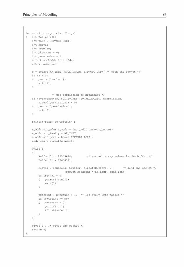
Principles of Modelling 89
int main(int argc, char **argv)
{ int Buffer[200];
int port = DEFAULT_PORT;
int retval;
int fromlen;
int pktcount = 0;
int permission = 1;
struct sockaddr_in s_addr;
int s, addr_len;
s = socket(AF_INET, SOCK_DGRAM, IPPROTO_UDP); /* open the socket */
if (s < 0)
{ perror("socket");
exit(1);
}
/* get permission to broadcast */
if (setsockopt(s, SOL_SOCKET, SO_BROADCAST, &permission,
sizeof(permission)) < 0)
{ perror("permission");
exit(2);
}
printf("ready to write\n");
s_addr.sin_addr.s_addr = inet_addr(DEFAULT_GROUP);
s_addr.sin_family = AF_INET;
s_addr.sin_port = htons(DEFAULT_PORT);
addr_len = sizeof(s_addr);
while(1)
{
Buffer[0] = 12345678; /* set arbitrary values in the buffer */
Buffer[1] = 87654321;
retval = sendto(s, &Buffer, sizeof(Buffer), 0, /* send the packet */
(struct sockaddr *)&s_addr, addr_len);
if (retval < 0)
{ perror("send");
exit(3);
}
pktcount = pktcount + 1; /* log every 50th packet */
if (pktcount >= 50)
{ pktcount = 0;
printf(".");
fflush(stdout);
}
}
close(s); /* close the socket */
return 0;
}

90 Principles of Flight Simulation
Program 2.2 readudp.c – a program to read UDPs
/* program to read UDPs */
#include <sys/types.h>
#include <sys/socket.h>
#include <netinet/in.h>
#include <stdio.h>
#include <termios.h>
#define DEFAULT_PORT 12345
#define DEFAULT_GROUP "255.255.255.255"
int main(int argc, char **argv)
{ int Buffer[200];
int port = DEFAULT_PORT;
int retval;
int fromlen;
int pktcount;
struct sockaddr_in s_addr;
int s;
int addr_len;
int permission = 1;
addr_len = sizeof(s_addr);
s_addr.sin_family = AF_INET;
s_addr.sin_addr.s_addr = htonl(INADDR_ANY);
s_addr.sin_port = htons(DEFAULT_PORT);
s = socket(AF_INET, SOCK_DGRAM, 0); /* open the socket */
if (s < 0)
{ perror("socket");
exit(1);
}
/* get permission to read broadcast packets */
if (setsockopt(s, SOL_SOCKET, SO_BROADCAST, &permission,
sizeof(permission)) < 0)
{ perror("permission");
exit(2);
}
/* bind the socket to its structure */
if (bind(s, (struct sockaddr *) &s_addr, sizeof(s_addr)) < 0)
{ perror("bind");
exit(2);
}
printf("ready to read\n");
while(1)
{
retval = recvfrom(s, Buffer, sizeof(Buffer), 0, /* get a packet */
(struct sockaddr *) &s_addr, &addr_len);

Principles of Modelling 91
if (retval < 0)
{ perror("recvfrom");
exit(4);
}
pktcount = pktcount + 1; /* log every 50th packet */
if (pktcount >= 50)
{ pktcount = 0;
printf(".");
fflush(stdout);
}
}
close(s); /* close the socket */
return 0;
}
2.11 A Real-time ProtocolThe flight simulator covered in this book runs on seven computers, as shown in Figure 2.33. Thepacket transfers are based on the UDP transfers described in Section 2.10. The nodes (computers)are assigned logical numbers 1–7, with corresponding IP addresses 192.168.1.1–192.168.1.7. Node1 acquires digital and analogue inputs and broadcasts a packet containing I/O data. Node 2 solvesthe equations of motion and broadcasts a packet containing aerodynamic and engine data. Node 3solves the navigation equations and broadcasts a packet containing navigation and avionics data.Node 4 is the instructor station and broadcasts the instructor commands and scripting information.Although it is possible to limit the instructor station transmissions to frames where the instructorissues a command, transmitting a packet for every frame simplifies the protocol considerably. Nodes5, 6 and 7 are the image generators; they are passive and do not broadcast any packets.
Node 1 sends its packet and waits for packets from nodes 2, 3 and 4. Node 2 waits for a packetfrom node 1, sends its packet and waits for packets from nodes 3 and 4. Node 3 waits for packetsfrom nodes 1 and 2, sends its packet and waits for a packet from node 4. Node 4 waits for packetsfrom nodes 1, 2 and 3 and then sends its packet. The visual system nodes (5, 6 and 7) wait fora packet from node 2, which contains sufficient information to render the frame. They are ableto perform their respective image generation tasks, before checking the information in the packetsfrom nodes 1, 3 and 4, for example, if the fogging level has changed.
The main requirement is to complete the transfers at the start of the frame, allowing as muchtime as possible for processing at each node. As the incoming packets are buffered, they can be
I/Ocomputer
Flightcomputer
Navigationcomputer
Instructorstation
Visualleft
channel
Visualcentre
channel
Visualright
channel
1 2 3 4 5 6 7
Figure 2.33 Simulator architecture

92 Principles of Flight Simulation
Figure 2.34 UDP transfers monitored by a network analyser
accessed at any time during the frame. In addition, node 1, the I/O computer runs at 50 Hz (20 msframe), providing a start-of-frame synchronisation for the other nodes and maintaining accurateframe timing.
Figure 2.34 is taken from a network analyser monitoring the network traffic during an autolandapproach. The fragment shows packet transfers 363–390, where the transmission time is given theleft-hand column. Note that the frames are transmitted at 20 ms intervals (50 Hz frame rate) andthat the order of transfers in each frame is 192.168.1.1, 192.168.1.2, 192.168.1.3 and 192.168.1.4.These transfers are typically completed in less than 750 µs, implying that the transfers occupy lessthan 1 ms (5%) at the start of the frame (with 100 Mbit/s Ethernet). Note also that the multicastbroadcast address is 192.168.1.255 (the destination address) and that the destination port is 12345.
The pseudo-code (on Page 94–95) summarises the packets transfers for each frame and theinitial values of the node states.
2.12 Problems in ModellingWe had already seen in Section 2.6 that the selection of inappropriate numerical methods canintroduce inaccuracy and possibly instability in the simulation of dynamic systems. Generally, theseeffects can be minimized if the time constants of a system are known, selecting an appropriate orderof the method and an appropriate step length for numerical integration. The step length determinesthe frame rate of the simulator, that is to say, the rate at which the solution is computed, for example,50 times per second. However, this value is bounded. If the step length is small, the number offrames to be computed per second may overload the processing capacity of the processor. For acoarse step length, in addition to the problems of accuracy and stability, it introduces one furtherproblem. At iteration rates below 20 Hz, discontinuities are just perceptible to the human operator; anapparently continuous system exhibits jerky motion. With perceivable delays, the human operatorwill over react to input stimuli in a simulator, behaving in a way that is very different frominteraction with the actual system. Although the model may be accurate, the errors arise from thecoarse step length. In applications where the step length is increased to reduce the computing load,care is needed to ensure that the frame rate does not drop below 20 Hz, for practical purposes.
A simulation is only as good as its model and any model depends on the data used to create themodel. While simple models can be created from an understanding of the underlying physics, more
Principles of Modelling 93
complex models are derived from physical models or measurements recorded on the actual system.Quite often, a physical model is based on assumptions and simplifications. For example, a windtunnel model of an aircraft will operate at very different values of Reynolds number (or airspeed) incomparison with the actual aircraft. The extrapolation of data derived in a wind tunnel experimentto the aircraft data may introduce inconsistencies. Quite often, it is difficult to take a large numberof measurements to cover the full operating range of a dynamic system and approximations mustbe made between measured points, introducing further inaccuracy. It may even be impracticableto obtain measurements over the operating regime of a dynamic system, for example, at the flightenvelope of an aircraft near its structural limits. Data may need to be interpolated between measuredpoints or extrapolated from a series of data points. Also, measurements may depend on severalvariables and it is impractical to take measurements to cover the full range of all the dependentvariables.
One further source of error arises from sensor errors. A sensor may not be linear, the resolution ofits measurement may be limited or the transducer providing the measurement may not be calibratedcorrectly. Some measurements can be taken in steady-state conditions, whereas others have to bederived from a continuous measurement. For example, in a wind tunnel, the aircraft can be fixedat a specific angle of attack, the wind speed set to a given value with the control surface deflectedto a measured angle. A load balance can measure the force on the model at this one setting ofthese three variables. Alternatively, it would be difficult to take an accurate measurement in a trialsaircraft, flying at a specific airspeed, attitude and elevator deflection. The alternative is to take aseries of input and output measurements but at fixed values of airspeed and altitude. In practice,it is difficult to fix specific variables in actual flight and flight trials are designed to minimize anyvariation in these forms of measurements. Furthermore, a parameter such as force can be measuredin a wind tunnel, whereas it has to be derived from other measurements in a flight trial.
Consequently, the acquisition of data using aircraft flight trials is very expensive. The aircraftmust be equipped with accelerometers, gyros and recording equipment and many hundreds of flighthours may be needed to acquire all the data. Moreover, the data then needs to be analysed andprocessed to provide the data in a form that can be used in a simulator. Not surprisingly, the datapackage for a civil transport aircraft may cost several million dollars.
There are other techniques to estimate the terms needed to model aircraft dynamics. In CFD, ifthe boundary conditions can be determined for a flow of liquid or gas, then the subsequent flow canbe determined in terms of the pressure, temperature and flow rate. The aircraft surface becomes oneof the boundaries of the flow and for given flight conditions, the analysis of the flow can be usedto determine lift and drag on an aircraft. The solution of the flow used in CFD methods can requirevery large amounts of processing, typically with a few seconds of flow data needing more than aday to compute with very fast processors. Although CFD methods are some 1000 times too slowfor real-time simulation, they are able to compute aircraft dynamics with high accuracy, particularlyin non-linear operating regions of the flight envelope. Their further advantage is that, in additionto the CFD software, they only require details of the aircraft 3D geometry to solve the equations.In practice, CFD methods are sensitive to the grid structures used to solve the flow equations.
An alternative approach to the CFD methods used to derive aircraft data is to use explicitequations based on the geometry and matched to experimental measurements, as used by Mitchell(1973) and Smetana (1984). For example, by comparing the drag curves of numerous aerofoils, agood prediction of drag can be deduced from the principle dimensions of the aerofoil. Such methodsare used in the Engineering Sciences Data series (ESDU, 2006). However, it must be rememberedthat these are approximation techniques and that the equations used may be simplified owing tolack of empirical data.
There is one further aspect of modelling data that it is easy to overlook. Once a model has beendeveloped, it needs to be validated. Most simulator data packages will provide extensive data tocheck simulator data against aircraft data, typically in the form of performance graphs or plots ofthe response of an aircraft to a specific input. It may be straightforward to replicate pilot responses
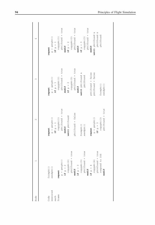
94 Principles of Flight Simulation
Node
12
34
Code
executed
each
frame
formpkt()
sendpkt()
repeat
p=getpkt()
ifp
=2
copypkt(2)
pkt2found=true
endif
ifp
=3
copypkt(3)
pkt3found=true
endif
ifp
=4
copypkt(4)
pkt4found=true
respondtoIOS
endif
repeat
p=
getpkt()
ifp
=1
copypkt(1)
pkt1found=true
endif
untilpkt1found
pkt1found=false
formpkt()
sendpkt()
repeat
p=
getpkt()
ifp
=3
copypkt(3)
pkt3found=true
repeat
p=getpkt()
ifp
=1
copypkt(1)
pkt1found=
true
endif
ifp
=2
copypkt(2)
pkt2found=
true
endif
untilpkt1found&
pkt2found
pkt1found=
false
pkt2found=
false
formpkt()
sendpkt()
repeat
p=getpkt()
ifp=
1
copypkt(1)
pkt1found=
true
endif
ifp=
2
copypkt(2)
pkt2found=
true
endif
ifp=
3
copypkt(3)
pkt3found=
true
endif
untilpkt1found&
pkt2found&
pkt3found

Principles of Modelling 95
Node
12
34
untilpk2tfound&
pkt3found&
pkt4found
pkt2found=
false
pkt3found=
false
pkt4found=
false
executeI/Ofunctions
waitforend-of-frame
endif
ifp
=4
copypkt(4)
pkt4found=true
respondto
IOS
endif
untilpkt3found&
pkt4found
pkt3found=false
pkt4found=false
executeflightmodel
repeat
if
p=
4
copypkt(4)
pkt4found=
true
respondtoIOS
endif
untilpkt4found
pkt4found=
false
executenavfunctions
pkt1found=
false
pkt2found=
false
pkt3found=
false
formpkt()
sendpkt()
executeIOSfunctions
Initial
values
pkt2found=
false
pkt3found=
false
pkt4found=
false
pkt1found=false
pkt3found=false
pkt4found=false
pkt1found=
false
pkt2found=
false
pkt4found=
false
pkt1found=
false
pkt2found=
false
pkt3found=
false

96 Principles of Flight Simulation
in a simulator (but not vice versa) and then the simulated response can be checked against theresponse from actual flight data. Of course, if the two sets of data correlate well, the simulatordesigner is confident that the simulator provides an accurate model of the aircraft dynamics. Thedifficulty arises where the two sets of data do not match. The simulator designer has to locate thesource of the inconsistency. However, with several variables depending on other variables, it isvery difficult to isolate the true cause of a problem. In particular, it is tempting to ‘tweak’ the datapackage to match the aircraft data or to use opinion from pilot assessments of a simulator to adjustthe model. The main problem is that changing the model in one place to ensure a good data match,may introduce errors in other areas of the model. This is a sensitive area for commercial airlines.If the simulator manufacturer matches the simulator responses to the corresponding aircraft data,but the airline pilots do not accept that the model has the appropriate handling characteristics, itmay not be clear where the change should be implemented. The simulator manufacturer is likelyto accept objective validation of the sets of data, whereas the airline may favour the subjectiveviews of its senior pilots during simulator acceptance. For this reason, the regulatory authoritiesare usually involved in the acceptance tests and validation of an airline flight simulator.
ReferencesBenyon, P.K. (1968) A review of numerical methods for simulation. Simulation , 11(5), 219– 238.Burns, A. and Wellings, A. (2001) Real-time Systems and Programming Languages , Pearson Educa-
tion.Cardullo, F.M., Kaczmarck, B. and Waycechowsky B.J. (1991) A comparison of several numerical
integration algorithms employed in real-time simulation. AIAA Flight Simulation TechnologiesConference, New Orleans.
ESDU (2006) Computer Program for Estimation of Aerofoil Characteristics at Subcritical Speeds:Lift-curve Slope, Zero-lift Incidence and Pitching Moment, Aerodynamic Centre and Drag PolarMinimum, Item 06020, Engineering Sciences Data, London.
Griffiths, D.V. and Smith, I.M. (1991), Numerical Methods for Engineers , Blackwell Scientific Pub-lications, Oxford.
Horowitz, P. and Hill W. (1989) The Art of Electronics , Cambridge University Press, Cambridge.Howe, R.M. (1989) An improved numerical integration method for flight simulation. AIAA Flight Sim-
ulation Technologies Conference, Technical Paper (A89-48376 21-09), Boston, MA, Washington,DC, 310– 316, http://www.aviationsystemsdivision.arc.nasa.gov/publications/hitl/rtsim/index.shtml
Howe, R.M. (1991) A new family of real-time predictor-corrector integration algorithms. Simulation ,57(3), 177– 186.
McFarland, R.E. (1997) Stability of Discrete Integration Algorithms for a Real-time, Second-orderSystem , NASA, Ames Research Centre.
Mitchell, C.G.B (1973) A Computer Programme to Predict the Stability and Control Characteristicsof Subsonic Aircraft , TR 73079, Royal Aircraft Establishment.
Murphy, J., Ridout, D. and Mcshane. B. (1988) Numerical Analysis, Algorithms and Computation ,Ellis Horwood Ltd., Chichester.
Press, W.H., Teukolsky, S.A. and Vetterling, W.T. (2007) Numerical Recipes: The Art of ScientificComputing , Cambridge University Press, Cambridge.
Smetana, F.O. (1984) Computer-assisted Analysis of Aircraft Performance Stability and Control ,McGraw Hill, New York.
Smith, M.J. (1979) Mathematical Modelling and Digital Simulation for Engineers and Scientists , JohnWiley & Sons, Ltd, New York.
Wood, M.B. (1992) An Improved Adams-Bashforth Numerical Integration Algorithm, DefenceResearch Agency, Report No. TMA&P7, Controller HMSO, London.
3Aircraft Dynamics
3.1 Principles of Flight ModellingEvery airline passenger, who has walked out onto an airport apron and looked up at the airlinerthey were about to board, must have had a momentary thought, wondering if such a large heavyaircraft would get off the ground, let alone fly several thousand miles. Despite such understandablereservations, the aerofoils of gliders, light aircraft, airships, helicopters, airliners, military jets,Concord and the Space Shuttle all generate sufficient lift for flight. Moreover, these aircraft can becontrolled by humans and computers and they are capable of transporting people or freight safelyover long distances at relatively high speed.
The principles of mechanics and fluid flows were established by Newton, Bernoulli, Euler,Lagrange and Laplace and then applied to aircraft dynamics by G. H. Bryan, F. W. Lanchester,H. B. Glauret, B. M. Jones and many others within a few years of the first flight by the Wrightbrothers. It was necessary to understand the aerodynamic forces produced during flight. First, theairframe had to withstand the applied forces. Secondly, an understanding of the aerodynamic forcesenabled faster or more efficient aircraft to be developed. Thirdly, the aircraft had to controlled bya pilot, implying an understanding of the dynamics of the aircraft.
Fortunately, for the flight simulator designer, many of the equations, which underpin the deriva-tion of aerodynamic forces, are well understood and can be applied to modelling the dynamicsof an aircraft. The purpose of this chapter is to understand how the flight simulator designer canapply these principles of aerodynamics and flight dynamics to develop an accurate model of thebehaviour of an aircraft, particularly its handling qualities, stability and performance. Building onthe concepts developed in Chapter 2, the equations that underpin aircraft motion will be developedto enable an aircraft model to be written as a software program.
Many of these equations are also used in modelling aircraft dynamics and more detailed deriva-tions are given in Etkin and Reid (1996), Boiffier (1998) and Stevens and Lewis (2003). However,it is important to appreciate that, in addition to the equations of motion, flight models require boththe data needed to construct the model and also the data to validate the model. Unfortunately, thisdata is expensive to acquire and, for operational aircraft, is a valuable asset to manufacturers andsimulator companies. Consequently, there are very few detailed flight models in the open literature.Often the data that is in the public domain lacks essential components and the reader is advisedto seek out many of the excellent National Aeronautics and Space Administration (NASA) reportssuch as Hanke’s (1971) model of the Boeing 747-100, Nguyen et al.’s (1979) model of the F-16Aand Heffley and Jewell’s (1972) report which contains rudimentary data for several aircraft.
Principles of Flight Simulation D. J. Allerton 2009, John Wiley & Sons, Ltd

98 Principles of Flight Simulation
3.2 The AtmosphereAircraft fly in the atmosphere, the gas that surrounds the earth. In this book, we will constrain theflight envelope to the troposphere, which is found up to an altitude of about 11,000 m. Admittedly,space vehicles and high altitude aircraft can fly higher into the stratosphere (and beyond). Althoughthe atmospheric properties can still be derived in the upper regions of the atmosphere, they arebeyond the scope of this book.
In the troposphere, air is considered to be a gas, obeying Boyle’s law in terms of the relationshipbetween pressure, temperature and density. Three quarters of the mass of the atmosphere is containedin the troposphere and is kept in place by the gravitational field of the earth. It is often assumedthat gravity is a constant, but the effects of the shape of the earth and the distribution of the massof the earth can affect the gravitational forces around the earth, as discussed in more detail inSection 3.3.5. Gravity is also affected by altitude, reducing as altitude increases. The effect of thelatter variation is that the geometric height of an aircraft (its altitude) also has a geopotential heightto take account of the reduction of gravitational force on the air particles where it is flying. Thegeopotential altitude is given by
h = R0z
R0 + z(3.1)
where h is the geopotential altitude, R0 is the earth radius (6,356,766 m) and z is the geometricaltitude. For example, if z = 11,000 m then h = 10,813 m; a reduction in altitude of 1.7%. Sucherrors are an important consideration for the simulator designer. Strictly, the geopotential altitudeshould be used to calculate temperature, pressure and density. Depending on the required fidelityof the simulator, it may be essential to model such effects or alternatively, these effects can beignored if they do not have any impact on training. Inevitably, there is a trade-off between theaccuracy of a model and the computational complexity of the model and this consideration appliesas much in modelling the atmosphere as it does to the modelling of aircraft dynamics.
Temperature varies with altitude, reducing as altitude increases in the troposphere. The rateat which the temperature reduces is known as temperature lapse and surprisingly, it is constantthroughout the troposphere. Temperature is given by
T = T0 − TLH (3.2)
where T is the temperature (◦K), T0 is the standard sea level temperature (◦K), TL is the temper-ature lapse and H is the geopotential altitude (metres). The lapse rate is constant at 0.0065 ◦ m−1.T0 is usually taken to be 288.15◦K (15 ◦C). At 11,000 m, the temperature will have dropped by71.5 to −56.5 ◦C. This calculation assumes dry air and of course, the temperature at sea level isnot always 15 ◦C. In computing the temperature, the temperature lapse is modified, so that dailyvariations of temperature at low altitude are included, with temperature reducing to the standardvalue of 216.65 ◦K at 11,000 m. Air temperature is particularly important in the modelling of engineperformance, having a significant effect on the performance of piston engines and jet engines.
Air pressure results from the mass of the column of air molecules above a unit area at a givenaltitude. Clearly, air pressure reduces as altitude increases. In the United States Standard AtmosphereModel, 1976 (Anon., 1976), the pressure is computed as follows:
P = P0eg0M0RsTL
ln(
T0T
)(3.3)
where P is the pressure (Pa), g0 is the acceleration of gravity (m/s2 at a latitude of 45 ◦), P0 is thepressure at g0 (Pa), M0 is the mean molecular weight of air (28.9644 kg/kmol), Rs is the gas constant
Aircraft Dynamics 99
(8314.32 Nm/kmol/◦K, TL is the temperature lapse rate (−0.0065 ◦/m), T0 is the temperature at sealevel (◦K) and T is the temperature (◦K).
Knowing the temperature and pressure of a gas, the density calculation is derived from thegas law
ρ = P
T· M0
Rs(3.4)
Air density reduces from 1.225 kg/m3 at sea level as altitude increases and is used in the computationof the aerodynamic forces and propulsive forces.
An alternative method of computing these terms is to use lookup tables derived from publishedtables of atmospheric data, interpolating between tabular values. However, the equations givenabove are straightforward to implement and are commonly used in simulation.
The speed of sound is also provided in an atmospheric model and depends on temperature
a =√
γ TRs
M0(3.5)
where a is the speed of sound (m/s) and γ is the ratio of specific heats for ideal diatomic gases(γ = 1.4). The speed of sound is used in the computation of the Mach number, which is neededfor aircraft displays and may also be used to derive aerodynamic coefficients needed for the flightmodel and the engine model. The Mach number is given by
M = V
a(3.6)
where M is the Mach number, V is the free stream velocity of the aircraft and a is the speed ofsound.
The program in Example 3.1 prints the values of temperature, pressure, density and speed ofsound from sea level to 10,800 m with close correspondence to the values given in the appendicesof McCormick (1995).
Example 3.1 Atmospheric model
/* atmos-1.c
computation of atmospheric temperature, pressure, density
based on the NASA implementation of the US Standard Atmosphere 1976
http://modelweb.gsfc.nasa.gov/atmos/us_standard.html
only valid for troposphere (sea-level to 36,000 ft) */
#include <stdio.h>
#include <stdlib.h>
#include <math.h>
const double Rs = 8314.32; /* Nm/(kmol K), gas constant */
const double M0 = 28.9644; /* kg/kmol, mean molecular weight of air */
const double g0 = 9.80665; /* m/s^2, accn of gravity at 45.5425 deg lat. */
const double r0 = 6356766.0; /* m, Earth radius at g0 */
const double P0 = 101325.0; /* Pa, air pressure at g0 */
const double T0 = 288.15; /* K, standard sea-level temperature */
const double Td = 273.15; /* K, 0 degrees C */

100 Principles of Flight Simulation
const double Gamma = 1.40; /* Ratio of Specific heats for an ideal
diatomic gas */
int main(int argc, char *argv[])
{
double As; /* constant */
int Z; /* geometric height m */
double H; /* geopotential height m */
double P; /* pressure Pa */
double T; /* temperature K */
double rho; /* density kg/m^3*/
double Cs; /* speed of sound m/s */
As = g0 * M0 / Rs;
for (Z=0; Z <= 10800; Z+=300)
{
H = r0 * (double) Z / (r0 + (double) Z);
T = T0 - 0.0065 * H;
P = P0 * exp(As * log(T0 / T) / (-0.0065));
rho = (P / T) * (M0 / Rs);
Cs = sqrt((Gamma * Rs / M0) * T);
printf("%5d %6.2f %8.4f %8.4f %6.2f\n", Z, T, P, rho, Cs);
}
}
Generally, an atmospheric model is based on the International Standard Atmosphere (ISA),with sea level conditions of temperature 15 ◦C, pressure 101,325 Pa and density 1.225 kg/m3. Itis necessary to compensate for any variation in sea level temperature or pressure in simulatingthe atmospheric conditions that prevail on a daily basis. For example, the take-off performanceof a light aircraft is significantly reduced on a hot day. Similarly, barometric pressures used insetting aircraft altimeters and air traffic control (ATC) clearances must also be replicated in a flightsimulator, particularly the variation of barometric pressure for QFE, QNH or standard altitude set-tings. Variations from ISA values are incorporated in outside air temperature gauges and altimetersin simulation. However, it is the absolute altitude of the centre of gravity (cg) of the simulatedaircraft that is used in all aerodynamic and propulsive computations, where density, pressure andtemperature values are derived from the equations above, modified to match the prevailing sea levelconditions.
3.3 Forces
3.3.1 Aerodynamic Lift
The density of air is so small in comparison with the density of an aircraft that it offers littlebuoyancy. However, if an aircraft is propelled through the air, the path taken by air moleculespassing over the aircraft wings may be different from the path taken by air molecules passingunder the aircraft wings, resulting in a pressure differential. By careful design of the wing profile,the net lower pressure above the wing is sufficient to produce an upward lifting force on the wingsof the aircraft. For a Boeing 747 aircraft accelerating along a runway, this pressure differential willbe capable of lifting a 300,000-kg aircraft off the ground at about 160 kt. This lift force will be

Aircraft Dynamics 111
whereCLW is the coefficient of lift of the wingCLT is the coefficient of lift of the tail
ST is the tail areaSW is the wing area
The term lST/cSW is a constant and can be replaced by V which is often referred to as the tailvolume coefficient giving
CM = CM0 + CL(h − h0) − V CLT (3.16)
In the steady-state, Cm = 0.Differentiating Equation 3.16 with respect to CL,
dCM
dCL= (h − h0) − V
dCLT
dCL(3.17)
Assuming the aircraft lift is proportional to the angle of incidence α, then the static stability isgiven by
dCM
dα= a(h − h0) − V
dCLT
dα(3.18)
where a is the gradient of the aircraft CL versus α curve.Moving the aircraft cg aft increases h , increasing the gradient of the dCM/dα curve and reducing
the static stability. The aircraft tail is designed so that dCM/dα is negative throughout the operatingrange of the aircraft and over the range of cg positions.
The neutral point is the position where the effect of the cg position is sufficient to give a dCM/dα
value of 0. The static margin is then the distance of the cg from the neutral point, normally expressedas a fraction of the wing mean chord c. Further analysis of this equation, for both stick-fixed andstick-free conditions is really the domain of the aircraft designer. A small static margin will givelight controls and a responsive aircraft but an aircraft that is easily disturbed from steady-stateflight. Although a large static margin provides a very stable aircraft, larger tail forces are needed tomanoeuvre the aircraft, which may not be acceptable, for example, where a good response is neededin the landing phase. For flight simulation, the aircraft geometry and aerodynamic derivatives areknown and the main requirement is to check the aircraft stability over the cg range publishedfor the aircraft. Methods of determining the stick-fixed neutral point in flight tests are covered inmost textbooks on aerodynamics. The (simulated) aircraft is flown at different cg positions and theelevator trim angle needed to trim the pitch attitude is measured and plotted against the coefficientof lift CL. The intersection of these curves coincides with the cg at the neutral point.
3.4.2 Aerodynamic Moments
The three primary controls: the elevator, the ailerons and the rudder are used by the pilot to select thedesired aircraft attitude. However, the change of motion can induce additional moments includingmoments resisting the applied motion. The magnitude of these moments is clearly influenced bythe geometry of the aircraft, for example, the size of the elevator surface but also depends on airdensity and airspeed. A point to bear in mind is that many of these terms are non-linear makinganalysis of the aircraft motion difficult or requiring linearization of the equations over a relativelysmall operating region.

112 Principles of Flight Simulation
The moments are computed in the stability axes and are defined by the following equations forthe moments in the roll, pitch and yaw axes, respectively:
Lstab = 1/2σV 2C sb(CLβ · β + CLδA · δa + CLδR · δr) + 1/4σVsb2(CLP · P + CLR · R) (3.19)
Mstab = 1/2σV 2C sc(CM0 + CMα · α + CMδE · δe) + 1/4σVsc2(CMQ · Q + CMα · α) (3.20)
Nstab = 1/2σV 2C sb(CNβ · β + CNδA · δa + CNδR · δr) + 1/4σVsb2(CNP · P + CNR · R) (3.21)
whereρ is air density
Vc is airspeedα is the angle of attackβ is the angle of sideslips is the wing areab is the wing spanc is the wing mean chord
δa is the aileron deflectionδe is the elevator deflectionδr is the rudder deflection
The coefficients Cab are known as the aerodynamic derivatives , where the subscript a denotesthe axis and the subscript b denotes the source of the moment term. Considerable care is neededin formulating these equations. Generally, the aerodynamic derivatives are non-dimensional, whichhas the advantage of compatibility between aerodynamic data derived in imperial units and dataproduced from terms defined in SI units. While this assumption is often valid, aerodynamic datamay be generated where the value of wing span b represents the wing semi-span rather than thefull wing span. In such cases, a spurious factor of 2 can be introduced into the equations. Thissituation is difficult to determine unless the method of dimensioning is clearly defined or if thereis sufficient test data provided to verify the equations. In some cases, dimensional aerodynamicderivatives are provided and the equivalent non-dimensional derivatives can be computed using thescale factors given in Table 3.1.
The aerodynamic derivatives constitute a major part of the data package for an aircraft. Eachderivative may be a function of several variables and data is normally provided in the form of aset of tables for each derivative or its primary components.
An alternative approach is to estimate the aerodynamic derivatives from empirical rules estab-lished for aircraft design or to use sources of data to predict these values. For example, EngineeringSciences Data Unit (ESDU) data sheets (ESDU, 1966) provide methods and tables to evaluate aero-dynamic derivatives for light aircraft. Similarly, Smetana (1984) provides the sources of data andthe methods used to predict these derivatives (including the Fortran programs). Mitchell (1973)also provides methods to estimate derivatives including swept wing fighter aircraft.
Table 3.1 Non-dimensional aerodynamic derivativesscale factors
Dimensional term Scale factor
CLβ , CLda, CLdr, CNβ , CNda, CNdr 1/2ρV 2sbCLp, CLr, CNp, CNr 1/4ρV sb2
CM0, CMα , CMde 1/2ρV 2scCMq, CMα
1/4ρV sc2
Aircraft Dynamics 113
3.4.3 Aerodynamic Derivatives
The validation of a flight model is covered in Chapter 7. If a step input is applied to the elevator(for example, moving the elevator control from its trimmed position backwards by 2 cm for onesecond, before returning the control to its original position), the resultant oscillatory pitching motiondepends on the coefficients in the pitching moment equations. The response in pitch over a fewseconds is known as the short period phugoid , whereas the response in pitch over a minute or sois known as the long period phugoid . Similarly, the response in yaw to a step input applied tothe rudder results in an oscillatory yawing motion, known as Dutch roll . The phugoid and Dutchroll response provide a unique ‘signature’ for an aircraft and are used to validate the equations ofmotion. In addition to the Dutch roll response, an aircraft also exhibits a spiral mode, which is thedegree to which a rolling motion induces further rolling motion. These terms also determine thespecific handling characteristics of an aircraft and the contribution of the individual aerodynamicderivatives to aircraft handling is summarized in Table 3.2.
One further term that is often included, particularly for propeller driven aircraft, is the additionalmoment resulting from interaction between the airflow from the propeller and the airframe. This isin addition to the direct moments resulting from the off-axis thrust, particularly in the pitch axis(for example, with under-slung engines) and the yaw axis with multi-engine aircraft. For low-wingsingle-engine aircraft, increasing power reduces the longitudinal stability but increases the direc-tional stability and elevator effectiveness. A NASA study using a full-scale wind tunnel (Fink andFreeman, 1969) provides a useful source to predict propeller effects for a light twin-engine aircraft.Wolowicz and Yancey (1972) predict the lateral-directional static and dynamic stability character-istics of a twin-engine aeroplane, including power effects. For aerobatic aircraft and turboprops,where the thrust to weight ratio is high, the effects of engine thrust can be significant at low speed(during take-off and landing) and considerable care is needed to model these effects. Similarly, forjet engine aircraft, the gyroscope effects of an engine can induce significant rolling and yawingmoments.
Several of these aerodynamic derivatives are dependent on the angle of attack. At high incidence,the airflow over the tail reduces and the effectiveness of the elevator and rudder may reducesignificantly. In addition, for jet aircraft, compressibility effects must be taken into account aboveMach 0.8. In practice, the accuracy of the aerodynamic data is a major contribution to the fidelityof the flight model. However, with so many derivatives, which are often combinations of half adozen components, in turn defined as a function of several variables, the scope for error is high andit can be very difficult to isolate an individual variable. For example, if the roll rate is insufficient,the cause may be an error in CLda or CLp. If the error is caused by too high damping, although theproblem may be reduced by increasing the aileron effectiveness, the modification may still resultin undesirable handling qualities. Consequently, considerable care is needed in the methods usedto acquire aircraft data, in the implementation of the flight model equations and most particularly,in the rigour of the verification of the flight model.
Most aircraft provide trim controls in pitch and yaw (and sometimes in roll). In the trimmed(non-accelerating) state, a trim control can relieve the force the pilot applies to the control column sothat the aircraft maintains the desired pitch attitude with zero pilot force (the ‘hands-off’ position).These trim controls are usually provided as tabs attached to the respective control surfaces and arecontrolled by a trim wheel in the cockpit, or in the case of large aircraft, by a small switch, whichactivates an electric motor to drive the trim tab. For an aircraft, movement of the elevator trim tabalters the mechanical trim datum. In a flight simulator, trimming either alters the elevator position,necessitating an irreversible mechanical trim linkage to move the column or, in the case of a fixedspring control loading, the trim input is added to the column position; in the trimmed state, theelevator control input is zero and the trim input provides an appropriate offset. As the trim effectvaries with airspeed, it is usually added to the respective control input rather than as an offsetto CM0.

114 Principles of Flight Simulation
Table 3.2 Aerodynamic derivatives
CM0 The contribution of the distribution of mass of the aircraft to the pitching moment. CM0
changes with the centre of gravity (cg) position and the effect of the flaps and undercarriageare often included in this term. The cg position depends on the mass and distribution of thefuel, crew, passengers and luggage and is usually quoted as a percentage of c.
CMα The major contribution to pitching stability. It determines the natural frequency of the shortperiod phugoid. It also determines the aircraft response to pilot inputs and gusts. The valueshould be sufficiently large to give an acceptable response to pilot inputs.
CMde This term is often referred to as ‘elevator effectiveness’ or ‘elevator power’. It is mainlyinfluenced by the area of the elevator surface and the angular range of movement of theelevator. The value should allow the pilot to control the aircraft safely in an evasivemanoeuvre or in response to a disturbance.
CMq As the aircraft pitches, resistance to the angular velocity is provided by this term. CMq iscommonly referred to a pitch damping as it dampens the short period phugoid. It provides amajor contribution to longitudinal stability and aircraft handling qualities.
CMα This derivative also contributes to damping of the short period phugoid.CLβ This derivative is known as the dihedral effect and counteracts the rolling motion induced by
sideslip, which dampens the Dutch roll mode and increases the spiral mode stability.CLda This term is also referred to as ‘aileron effectiveness’ and depends on the surface area and the
range of movement of the ailerons. Roll rate is proportional to aileron deflection. Withdifferential ailerons care is needed to ensure that the data relates to the net contribution ofailerons. Aircraft may have both inboard and outboard ailerons requiring separate data for thecontribution of each aileron. In addition, spoilers can also be used to provide roll inputs.
CLdr Movement of the rudder induces both a yawing moment and a rolling moment. Generally, thisterm is small and is often neglected.
CLp This term represents resistance to rolling motion as an aircraft banks, providing damping of theDutch roll mode.
CLr As an aircraft yaws, the induced rolling moment is damped out by this term. Its major effect ison the spiral mode and consequently, the term is usually a small positive value.
CNβ If the aircraft is disturbed in yaw, this term provides a resistance to the yawing motion andconsequently, is often referred to as the ‘weathercock’ derivative and is mostly dependent onthe geometry of the aircraft tail. The term determines the natural frequency of the Dutch rolland affects the spiral stability of the aircraft.
CNda As aileron input is introduced, the aircraft may also tend to yaw, caused mostly by the drag ofthe aileron deflections on each wing. (The term adverse yaw is used if this value contributesa yawing moment in the direction opposite to the implied direction of banking). Typically,this value is very small or zero, particularly with differential ailerons.
CNdr This term is also referred to as ‘rudder effectiveness’ and depends on the surface area andrange of movement of the rudder. Generally, the rudder is used to counteract sideslip and tocoordinate turns, so that the effect of this derivative influences the handing qualities.
CNp This derivate gives the change in yawing moment resulting from roll. Large positive valuesincrease the Dutch roll damping.
CNr This term is the main contributor to damping in yaw. Its effect is to damp the Dutch roll and toincrease spiral mode stability.
3.5 Axes SystemsIn the previous sections, in discussing the forces and moments applied to an aircraft, referenceswere made to the aircraft axes and also to the earth axes. The aerodynamic, propulsive and gravita-tional forces on an aircraft, which are typically derived from data packages, are most convenientlycomputed in the aircraft frame. However, an aircraft may be at 5000 or 20,000 ft; it may be flyinglevel or inverted or banked at 60 ◦. Just knowing the forces and therefore the resultant motion ofthe aircraft in the aircraft axes is not particularly useful; the attitude, position, altitude, heading and
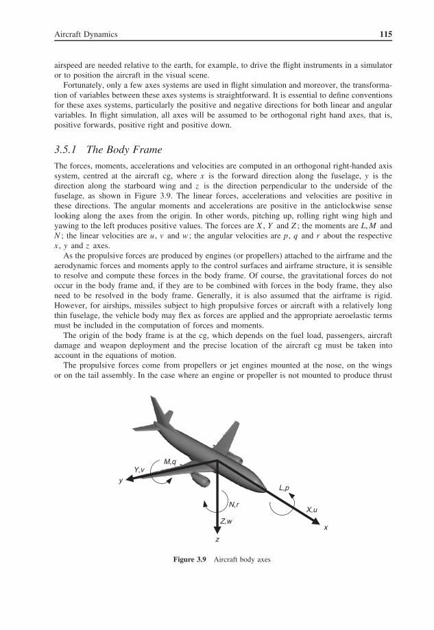
Aircraft Dynamics 115
airspeed are needed relative to the earth, for example, to drive the flight instruments in a simulatoror to position the aircraft in the visual scene.
Fortunately, only a few axes systems are used in flight simulation and moreover, the transforma-tion of variables between these axes systems is straightforward. It is essential to define conventionsfor these axes systems, particularly the positive and negative directions for both linear and angularvariables. In flight simulation, all axes will be assumed to be orthogonal right hand axes, that is,positive forwards, positive right and positive down.
3.5.1 The Body Frame
The forces, moments, accelerations and velocities are computed in an orthogonal right-handed axissystem, centred at the aircraft cg, where x is the forward direction along the fuselage, y is thedirection along the starboard wing and z is the direction perpendicular to the underside of thefuselage, as shown in Figure 3.9. The linear forces, accelerations and velocities are positive inthese directions. The angular moments and accelerations are positive in the anticlockwise senselooking along the axes from the origin. In other words, pitching up, rolling right wing high andyawing to the left produces positive values. The forces are X , Y and Z ; the moments are L, M andN ; the linear velocities are u , v and w ; the angular velocities are p, q and r about the respectivex , y and z axes.
As the propulsive forces are produced by engines (or propellers) attached to the airframe and theaerodynamic forces and moments apply to the control surfaces and airframe structure, it is sensibleto resolve and compute these forces in the body frame. Of course, the gravitational forces do notoccur in the body frame and, if they are to be combined with forces in the body frame, they alsoneed to be resolved in the body frame. Generally, it is also assumed that the airframe is rigid.However, for airships, missiles subject to high propulsive forces or aircraft with a relatively longthin fuselage, the vehicle body may flex as forces are applied and the appropriate aeroelastic termsmust be included in the computation of forces and moments.
The origin of the body frame is at the cg, which depends on the fuel load, passengers, aircraftdamage and weapon deployment and the precise location of the aircraft cg must be taken intoaccount in the equations of motion.
The propulsive forces come from propellers or jet engines mounted at the nose, on the wingsor on the tail assembly. In the case where an engine or propeller is not mounted to produce thrust
L,p
x
z
y
N,r
Z,w
X,u
M,qY,v
Figure 3.9 Aircraft body axes

116 Principles of Flight Simulation
in line with the x axis, this alignment will be known, enabling the appropriate components to beresolved in the body axes. Similarly, the moments generated by the engines can be computed fromthe thrust produced and the distance from an axis, for example, to produce a pitching moment forunder-slung engines or a yawing moment for multi-engine aircraft.
The cg of an aircraft follows a trajectory known as the flight path . At any instant, the flight pathangle γ is the angle the flight path makes with respect to the surface of the earth. It is importantto appreciate that the aircraft may not necessarily be pointing in the direction of the flight path. Inother words, the pitch attitude θ and the flight path angle γ will differ by the angle of attack andsimilarly, yaw attitude ψ and the track angle will differ by the angle of sideslip. Figure 3.10 showsthe relationship between the pitch and flight path angles; in this example, the aircraft is showndescending and the angles are deliberately exaggerated.
For any flight path angle
γ = θ − α (3.22)
where α is the aircraft angle of attack.In the case of level flight, γ = 0 and θ = α. In climbing flight, the aircraft may be climbing
at 5 ◦ say, with an angle of attack of 8 ◦, giving a pitch attitude of 13 ◦. As most aircraft are notfitted with an angle of attack gauge and although the flight path angle could be calculated from theairspeed and vertical rate of climb, pilots select recommended power settings and pitch attitudes toachieve the desired flight path angle.
In simulation, the angle of attack is needed to compute the aerodynamic forces and moments andthe pitch attitude in needed in axes transformations, for the artificial horizon instrument display andfor the visual system computations. The flight path angle is mostly used in flight control systems.The variables u , v and w , defined in the aircraft body axes, are used in the computation of theoverall aircraft speed and the angle of attack, as follows:
Vc =√
u2 + v 2 + w2 (3.23)
α = tan−1(w
u
)(3.24)
where Vc is the speed of the cg of the aircraft along its flight path and α is the angle of attack. Forsmall angle approximations, where α ≈ tan(α)
α = uw − wu√u2 + w2
(3.25)
For lateral motion, the aircraft flight path results in a track over the ground. In the presence ofwind, or during banked flight, or as a result of rudder inputs or if there is an imbalance in engine
qa
g
Pitch
Flight path
Figure 3.10 Flight path angle
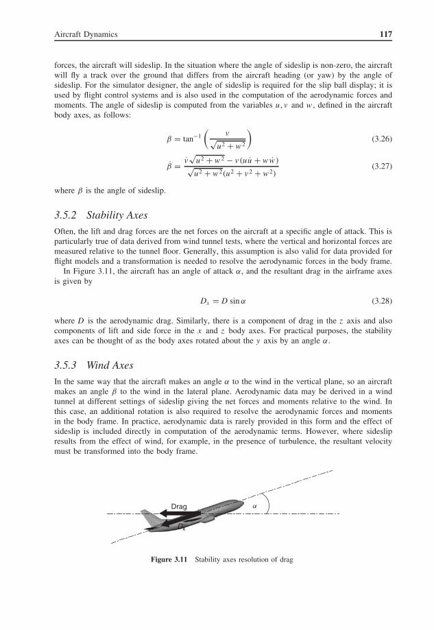
Aircraft Dynamics 117
forces, the aircraft will sideslip. In the situation where the angle of sideslip is non-zero, the aircraftwill fly a track over the ground that differs from the aircraft heading (or yaw) by the angle ofsideslip. For the simulator designer, the angle of sideslip is required for the slip ball display; it isused by flight control systems and is also used in the computation of the aerodynamic forces andmoments. The angle of sideslip is computed from the variables u , v and w , defined in the aircraftbody axes, as follows:
β = tan−1(
v√u2 + w2
)(3.26)
β = v√
u2 + w 2 − v(uu + ww)√u2 + w2(u2 + v 2 + w2)
(3.27)
where β is the angle of sideslip.
3.5.2 Stability Axes
Often, the lift and drag forces are the net forces on the aircraft at a specific angle of attack. This isparticularly true of data derived from wind tunnel tests, where the vertical and horizontal forces aremeasured relative to the tunnel floor. Generally, this assumption is also valid for data provided forflight models and a transformation is needed to resolve the aerodynamic forces in the body frame.
In Figure 3.11, the aircraft has an angle of attack α, and the resultant drag in the airframe axesis given by
Dx = D sin α (3.28)
where D is the aerodynamic drag. Similarly, there is a component of drag in the z axis and alsocomponents of lift and side force in the x and z body axes. For practical purposes, the stabilityaxes can be thought of as the body axes rotated about the y axis by an angle α.
3.5.3 Wind Axes
In the same way that the aircraft makes an angle α to the wind in the vertical plane, so an aircraftmakes an angle β to the wind in the lateral plane. Aerodynamic data may be derived in a windtunnel at different settings of sideslip giving the net forces and moments relative to the wind. Inthis case, an additional rotation is also required to resolve the aerodynamic forces and momentsin the body frame. In practice, aerodynamic data is rarely provided in this form and the effect ofsideslip is included directly in computation of the aerodynamic terms. However, where sideslipresults from the effect of wind, for example, in the presence of turbulence, the resultant velocitymust be transformed into the body frame.
aDrag
Dx
Figure 3.11 Stability axes resolution of drag

118 Principles of Flight Simulation
3.5.4 Inertial Axes
An aircraft is subject to both internal and external forces. Its subsequent motion could be definedwith respect to some fixed point in space. If this point is the origin of a set of axes that are fixedand non-rotating, then this frame is termed an inertial frame and strictly, Newton’s Laws of Motionare only valid in an inertial frame. In practice, inertial frames are difficult to visualize for aircraftmotion, although their concept can help to simplify the computations used in aircraft navigation.
The definition can be relaxed to define an axis system that is only fixed and non-rotating withrespect to a moving object. For example, the concrete floor of a building housing the motionplatform of a flight simulator is an inertial frame. It is fixed at all times with respect to the platformactuators. The platform actuators and the simulator platform move with respect to a fixed point onthe concrete floor.
With some simplification, inertial navigation frames can be used in flight simulation. For example,if a flight simulation is based on a single airfield and the aircraft only flies some 50 miles or sofrom this airfield, the aircraft motion could be defined relative to the airfield coordinates. In effect,this is a ‘flat earth’ simplification, ignoring the curvature of the earth. If an aircraft flies on aconstant heading between two points of the surface of this flat earth, the flight path is a straightline over the surface of the earth. Whereas, the shortest distance from New York to London is atrack along a great circle route, where the aircraft heading would change continuously from NewYork to London.
The earth can be treated as an inertial frame. However, it rotates with respect to its axes (every24 hours) and with respect to the sun, approximately every 365 days. There is a further complication;as the earth is spherical, flying at a constant altitude should result in a curved flight path, parallelto the curved surface of the earth, rather than a straight line in space. In addition, the relativelyslow turn rate of the earth should also be taken into account, particularly to compute the motionof an aircraft for long distance flights.
Although it is straightforward to compute forces, moments, accelerations and velocities (linearand angular) in body axes, it is also necessary to transform this motion to velocity and positionrelative to the earth, which can be treated as an inertial frame so that Newton’s Laws of Motionapply, enabling aircraft position, velocity and attitude to be referenced to the earth frame.
3.5.5 Transformation between Axes
The transformation of a point or vector can be thought of as either a rotation of the axes orthe rotation of the point in the original frame. In either case, the point is transformed from thecoordinates of the original frame to coordinates of the new frame. In two dimensions, a vector canbe rotated, as shown in Figure 3.12. If the point is rotated in a counter clockwise direction aboutthe origin by an angle θ
x ′ = x cos θ − y sin θ (3.29)
y ′ = x sin θ + y cos θ (3.30)
The same equation would also apply if the axes were rotated clockwise by an angle θ , where x ′ andy ′ are the coordinates in the rotated frame. If the points (x , y) and (x ′, y ′) are treated as vectors,then rotation can be defined by a simple matrix operation:[
x ′y ′
]=
[cos θ − sin θ
sin θ cos θ
] [xy
](3.31)
The method is easily extended to rotations in three dimensions, but the results are simply stated inthe following section; formal derivations are given in most textbooks on the subject.
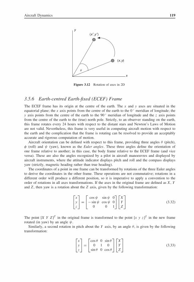
Aircraft Dynamics 119
x
y
(x ,y)
(x ′,y ′)
q
Figure 3.12 Rotation of axes in 2D
3.5.6 Earth-centred Earth-fixed (ECEF) Frame
The ECEF frame has its origin at the centre of the earth. The x and y axes are situated in theequatorial plane; the x axis points from the centre of the earth to the 0 ◦ meridian of longitude; they axis points from the centre of the earth to the 90 ◦ meridian of longitude and the z axis pointsfrom the centre of the earth to the (true) north pole. Strictly, to an observer standing on the earth,this frame rotates every 24 hours with respect to the distant stars and Newton’s Laws of Motionare not valid. Nevertheless, this frame is very useful in computing aircraft motion with respect tothe earth and the complication that the frame is rotating can be resolved to provide an acceptablyaccurate and rigorous computation of motion.
Aircraft orientation can be defined with respect to this frame, providing three angles θ (pitch),φ (roll) and ψ (yaw), known as the Euler angles . These three angles define the orientation ofone frame relative to another; in this case, the body frame relative to the ECEF frame (and viceversa). These are also the angles recognized by a pilot in aircraft manoeuvres and displayed byaircraft instruments, where the attitude indicator displays pitch and roll and the compass displaysyaw (strictly, magnetic heading rather than true heading).
The coordinates of a point in one frame can be transformed by rotations of the three Euler anglesto derive the coordinates in the other frame. These operations are not commutative; rotations in adifferent order will produce a different position, so it is imperative to apply a convention to theorder of rotations in all axes transformations. If the axes in the original frame are defined as X , Yand Z , then yaw is a rotation about the Z axis, given by the following transformation:
x
yz
=
cos ψ sin ψ 0
− sin ψ cos ψ 00 0 1
X
YZ
(3.32)
The point [X Y Z ]T in the original frame is transformed to the point [x y z ]T in the new framerotated (in yaw) by an angle ψ .
Similarly, a second rotation in pitch about the Y axis, by an angle θ , is given by the followingtransformation:
x
yz
=
cos θ 0 sin θ
0 1 0sin θ 0 cos θ
X
YZ
(3.33)

120 Principles of Flight Simulation
Finally, a third rotation in roll about the X axis, by an angle φ, given by:
x
y
z
=
1 0 0
0 cos φ sin φ
0 − sin φ cos φ
X
Y
Z
(3.34)
To combine all three rotations, the transformations in yaw, then pitch, then roll can be describedby a single matrix transformation, given by the product of the three matrices in the correctorder:
x
y
z
=
cos ψ sin ψ 0
− sin ψ cos ψ 0
0 0 1
cos θ 0 sin θ
0 1 0
sin θ 0 cos θ
1 0 0
0 cos φ sin φ
0 − sin φ cos φ
X
Y
Z
(3.35)
Giving
x
y
z
=
cos ψ cos θ sin ψ cos θ − sin φ
cos ψ sin θ sin φ − sin ψ cos φ cos ψ cos φ + sin ψ sin θ sin φ cos θ sin φ
cos ψ sin θ cos φ + sin ψ sin φ sin ψ sin θ cos φ − cos ψ sin φ cos θ cos φ
X
Y
Z
(3.36)
A matrix to transform between axes is often referred to as a direction cosine matrix (DCM). Inthis case, the DCM enables a vector in the earth frame [X Y Z ]T to be computed in the aircraftbody frame. It is used in flight dynamics to transform velocities in the body frame to the earthframe. It can also be used to transform earth frame velocities (e.g. wind velocity) to the body frame.It is also used in visual system computations to transform a point (or polygon) defined in earthcoordinates to a coordinate frame in the pilot eye frame, aligned to the body frame.
One example where this transformation is used is to compute the gravitational component of forcein the body axes of an aircraft. In the earth frame, gravitational force is given by [0 0 mg]T (wherem is the aircraft mass and g is gravitational acceleration); the three components are computed inthe body frame as follows:
Fx
Fy
Fz
=
cos ψ cos θ sin ψ cos θ − sin φ
cos ψ sin θ sin φ − sin ψ cos φ cos ψ cos φ + sin ψ sin θ sin φ cos θ sin φ
cos ψ sin θ cos φ + sin ψ sin φ sin ψ sin θ cos φ − cos ψ sin φ cos θ cos φ
0
0
mg
(3.37)
giving
Fx = −mg sin φ (3.38)
Fy = mg cos θ sin φ (3.39)
Fz = mg cos θ cos φ (3.40)
It is important to appreciate the range of the Euler angles:
−π ≤ ψ ≤ +π (3.41)
−π ≤ φ ≤ +π (3.42)
−π/2 ≤ θ ≤ +π/2 (3.43)
Aircraft Dynamics 121
It is not obvious that pitch should be constrained to the range ±90 ◦. Consider a loop; as the pilotpulls up into the loop, the pitch increases to 80 ◦, then 85 ◦, 86 ◦, 87 ◦, 88 ◦ and 89 ◦. At this point,the aircraft is still pointing forwards, but almost vertically upwards. In the next two degrees ofmotion, the aircraft passes through 90 ◦ and subsequently is pointing backwards, but at 89 ◦ to thehorizon. Notice also that during this manoeuvre, as the pitch angle passes through 90 ◦, the aircraftheading changes from forwards to backwards (an 180 ◦ instantaneous change in yaw) and also, theaircraft changes from upright to inverted (an 180 ◦ instantaneous change in roll).
Although at first sight this notation looks cumbersome, it provides a very powerful mechanismto transform a vector from one axis system to another, or between any sets of orthogonal axes.These matrix transformations can be combined as a series of transformations that are representedby a single transformation matrix.
There is one further benefit of this approach; although the reverse transformation implies matrixinversion, this operation is achieved by transposing the transformation matrix.
If
x
yz
= [A]
X
YZ
, then
X
YZ
= [A]T
x
yz
(3.44)
For example, the transformation between the body frame velocities (u , v , w ) and the earth framevelocities (VN, VE, Vd), where VN is the velocity in the north direction, VE is the velocity in theeast direction and Vd is the velocity in the downward direction, is given by:
VN
VE
Vd
=
cos ψ cos θ cos ψ sin θ sin φ − sin ψ cos φ cos ψ sin θ cos φ + sin ψ sin φ
sin ψ cos θ cos ψ cos φ + sin ψ sin θ sin φ sin ψ sin θ cos φ − cos ψ sin φ
− sin θ cos θ sin φ cos θ cos φ
u
vw
(3.45)
The angular velocities can be transformed between the body and the earth frames using a similarapproach, noting that the derivation also uses the Euler angles. The body rates are given by:
p
qr
=
1 0 − sin θ
0 cos φ cos θ sin φ
0 − sin φ cos θ cos φ
φ
θ
ψ
(3.46)
The reverse transformation, to derive the Euler angle rates from the body rates, is given by thetransformation:
φ
θ
ψ
=
1 sin φ tan θ cos φ tan θ
0 cos φ − sin φ
0 sin φ sec θ cos φ sec θ
p
qr
(3.47)
which expands to the following well-known equations:
φ = p + q sin φ tan θ + r cos φ tan θ (3.48)
θ = q cos φ − r sin φ (3.49)
ψ = q sin φ sec θ + r cos φ sec θ (3.50)
Notice that these equations contain a singularity when θ = −π/2 or θ = +π/2, where the termstan θ and sec θ are infinite. Such conditions occur in aerobatic manoeuvres where the aircraft

122 Principles of Flight Simulation
loops or climbs at a near vertical angle. Two techniques are used to overcome these problems. Thepitch angle can be constrained so that the computation results in a valid floating point number.For example, tan(89.5 ◦) = 114.6 and this value could be substituted in computations when thepitch attitude is between 89.5 ◦ and 90.5 ◦. The numerical error introduced by this approximationonly occurs at this extreme flight attitude where its effects on the aircraft behaviour may not beapparent. The more rigorous and commonly used method is to use quaternions, which are describedin Section 3.6.
3.5.7 Latitude and Longitude
In flight simulation, airfields, geographic features and navigation beacons are defined by theirlatitude and longitude. Consequently, it is common for aircraft position to be defined by latitudeand longitude rather than a position relative to a fixed datum. Assuming that the earth is a perfectsphere and ignoring any variation in gravity over the surface of the earth, the equations to derivelatitude rate and longitude rate are given by:
λ = Vn
R + hλ =
∫λ dt (3.51)
µ = Ve sec λ
R + hη =
∫µ dt (3.52)
h = −Vd h =∫
h dt (3.53)
where λ is latitude, µ is longitude, R is the radius of the earth and h is the altitude above mean sealevel. Note the singularity as λ approaches −90 ◦ or +90 ◦, which occurs flying directly over thenorth or south poles. Care is needed to cope with this problem, although in practice, few simulatorsare likely to be used to practice take-offs or landings near the poles.
Care is also needed with the precision of the computation of latitude and longitude. The rangeof latitude is ±90 ◦ (±π /2) and the range of longitude is ±180 ◦ (±π). A standard 32-bit floatingpoint variable typically has 8 bits for the exponent and 24 bits for the mantissa. For numbers inthe range used to compute latitude and longitude, this corresponds to an accuracy of approximately10−7. For an earth circumference of approximately 40 × 106 m, the floating point resolution isof the order 4 m. In other words, the smallest movement of an aircraft may be as high as 4 m,which would result in unacceptably jerky motion in the visual system as an aircraft taxies slowly.To avoid such problems, double precision (64-bit) floating point arithmetic is normally used in thecomputation of latitude and longitude.
3.6 QuaternionsQuaternions (also known as the four-parameter method ) are widely used in flight simulation (Fangand Zimmerman, 1969). They enable the Euler angles to be computed but avoid the singularity inthe computation of the body rates in Equations 3.48–3.50. The four quaternion parameters e0, e1, e2
and e3 are defined, in terms of the Euler angles, as follows:
e0 = cosψ
2cos
θ
2cos
φ
2+ sin
ψ
2sin
θ
2sin
φ
2(3.54)
e1 = cosψ
2cos
θ
2sin
φ
2− sin
ψ
2sin
θ
2cos
φ
2(3.55)

Aircraft Dynamics 123
e2 = cosψ
2sin
θ
2cos
φ
2+ sin
ψ
2cos
θ
2sin
φ
2(3.56)
e3 = sinψ
2cos
θ
2cos
φ
2− cos
ψ
2sin
θ
2sin
φ
2(3.57)
These identities can be used to initialize the quaternion values. At all times, the quaternion param-eters must satisfy the following constraint:
e20 + e2
1 + e22 + e2
3 = 1 (3.58)
The quaternion parameters are formed from the body rates as follows:
e0 = −1
2(e1p + e2q + e3r) e0 =
∫e′
0 (3.59)
e1 = 1
2(e0p + e2r − e3q) e1 =
∫e′
1 (3.60)
e2 = 1
2(e0q + e3p − e1r) e2 =
∫e′
2 (3.61)
e3 = 1
2(e0r + e1q − e2p) e3 =
∫e′
3 (3.62)
The DCM used to transform velocities in the body frame can be defined in terms of the quaternionparameters, as follows:
e20 + e2
1 − e22 − e2
3 2(e1e2 − e0e3) 2(e0e2 + e1e3)
2(e1e2 + e0e3) e20 − e2
1 + e22 − e2
3 2(e2e3 − e0e1)
2(e1e3 − e0e2) 2(e2e3 + e0e1) e20 − e2
1 − e22 + e2
3
=
a11 a12 a13
a21 a22 a23
a31 a32 a33
(3.63)
Combining elements from the DCM given in terms of the Euler angles enables the Euler angles tobe computed:
θ = sin−1(−a31) (3.64)
φ = tan−1(
a32
a33
)(3.65)
ψ = tan−1(
a21
a11
)(3.66)
where a denotes the elements of the DCM. Note that this representation also depends on thenumerical accuracy of the integration algorithm and that the magnitude of the quaternion values mustbe continually adjusted to satisfy the constraint in Equation 3.58, which is applied by modifyingthe computation of the quaternion parameter rates, as follows:
e0 = −1
2(e1p + e2q + e3r) + kλe0 (3.67)
e1 = 1
2(e0p + e2r − e3q) + kλe1 (3.68)

124 Principles of Flight Simulation
e2 = 1
2(e0q + e3p − e1r) + kλe2 (3.69)
e3 = 1
2(e0r + e1q − e2p) + kλe3 (3.70)
where kh ≤ 1, λ = 1 − (e20 + e2
1 + e22 + e2
3 ) and h is the integration step length (frame rate). Thismethod, known as the method of algebraic constraint , where λ is adjusted during each iteration,ensures that the constraint is maintained. Quaternions are widely used in flight simulation, particu-larly in military simulators where aerobatic manoeuvres are practised. However, care must be takento initialize the quaternion parameters and to ensure that the numeric constraint outlined above isnot violated.
3.7 Equations of MotionIn the previous sections, we have reviewed how the forces and moments on an aircraft can bederived and how terms computed in one axis system can be transformed to a more convenient axissystem. In this section, we look at the equations which underpin aircraft motion. In particular, anaircraft has six degrees of freedom, translating and rotating in three linear dimensions and threeangular dimensions (Fogarty and Howe, 1969).
Recalling the axes shown in Figure 3.9, the axes conventions and primary terms are summarizedin Table 3.3.
The aircraft forces are given by:
∑Fx = d
dt(mu) (3.71)
∑Fy = d
dt(mv) (3.72)
∑Fz = d
dt(mw) (3.73)
The aircraft moments are given by:
∑L = dhx
dt(3.74)
∑M = dhy
dt(3.75)
∑N = dhz
dt(3.76)
Consider an element of mass dm rotating at an angular velocity � , where � = pi + qj + rk , asshown in Figure 3.13.
Table 3.3 Axes notation
Axis Linear velocity Angular velocity Moment Force Moment of momentum Moment of inertia
X U P L Fx hx Ixx
Y V Q M Fy hy Iyy
Z W R N Fz hz Izz

Aircraft Dynamics 125
x
yz
QR
PU
V
W
∆m
Figure 3.13 Forces on an element of mass
x x
z
(a) (b)
y
Q R
Side on view View from above
Figure 3.14 Linear velocity components
Consider the velocity in the x direction as shown in Figure 3.14. The pitching rate Q contributesQz and the yawing rate contributes −Ry . Clearly, the roll rate term contributes no velocity alongthe x axis. Recalling that the x axis is forwards, the y axis is in the direction of the right wingand the z axis is down, then the linear velocity components of �m in the x , y and z directions,respectively, are given by:
x = U + Qz − Ry (3.77)
y = V − Pz + Rx (3.78)
z = W + Py − Qx (3.79)
Differentiating Equations 3.77–3.79 to derive the accelerations:
x = U + Qz + Qz − Ry − Ry (3.80)
y = V − P z − Pz + Rx + Rx (3.81)
z = W + Py + Py − Qx − Qx (3.82)
126 Principles of Flight Simulation
Substituting for x , y and z from Equations 3.77–3.79
x = U + QW + QPy − Q2x − RV + RPz − R2x + Qz − Ry (3.83)
y = V − PW − P2y − PQx + RU + RQz − R2y − P z + Rx (3.84)
z = W + PV − P2z + PRx − QU − Q2z + QRy + Py − Qx (3.85)
The inertia forces of the mass element are given by:
Fxi = −mx (3.86)
Fyi = −my (3.87)
Fzi = −mz (3.88)
The inertia moments of the mass element are given by:
Mxi = Fzi y − Fyi z (3.89)
Myi = Fxi − Fzi x (3.90)
Mzi = Fyi x − Fxi y (3.91)
The total inertia forces and moments acting on the aircraft are obtained by summingEquations 3.86–3.91 over the total aircraft mass. However, several terms vanish if the originis taken as the cg, in particular:
∑�mx = 0 (3.92)∑�my = 0 (3.93)∑�mz = 0 (3.94)∑
�mxy = 0 (3.95)∑�myz = 0 (3.96)
(��mxy and ��myz are assumed to be zero if the aircraft is symmetric about the xz plane).The moments of inertia are defined as:
Ixx =∑
�m(y2 + z 2) (3.97)
Iyy =∑
�m(x 2 + z 2) (3.98)
Izz =∑
�m(x 2 + y2) (3.99)
Ixz =∑
�mxz (3.100)
Although the moments of inertia could be computed from these summations, as the geometry andmaterial of the aircraft is known, these values are usually determined during aircraft manufacture,
Aircraft Dynamics 127
from the mass distribution of the aircraft. The forces are determined from Equations 3.83–3.85,eliminating the terms containing mx, my and mz :
Fx = mx = m(U + QW − RV ) (3.101)
Fy = my = m(V − PW + RU ) (3.102)
Fz = mz = m(W + PV − QU ) (3.103)
Similarly, Equations 3.89–3.91 can be expanded, substituting the terms in Equations 3.83–3.85 toprovide the moments:
L = Ix P + QR(Iz − Iy ) − Iyz (Q2 − R2) − Ixz (R + PQ) − Ixy (Q − PR) (3.104)
M = Iy Q + PR(Ix − Iz ) + Ixz (P2 − R2) − Iyz (R − PQ) − Ixy (P + QR) (3.105)
N = Iz R + PQ(Iy − Ix ) − Ixy (P2 − Q2) − Ixz (P − QR) − Iyz (Q + PR) (3.106)
If the aircraft has a symmetrical distribution of mass in the fore and aft plane of geometry, whichis the case for most aircraft, then Ixz = 0 and Iyz = 0 and Equations 3.104–3.106 reduce to:
L = Ix P + QR(Iz − Iy ) − Ixz (R + PQ) (3.107)
M = Iy Q + PR(Ix − Iz ) + Ixz (P2 − R2) (3.108)
N = Iz R + PQ(Iy − Ix ) − Ixz (P − QR) (3.109)
These equations ignore the gyroscopic effects of propellers, rotor blades and rotating turbines. If hdenotes the angular momentum vector, defined in the body axes, then:
L = Ix P + QR(Iz − Iy ) − Ixz (R + PQ) + Qhz − Rhy (3.110)
M = Iy Q + PR(Ix − Iz ) + Ixz (P2 − R2) − Phy + Rhx (3.111)
N = Iz R + PQ(Iy − Ix ) − Ixz (P − QR) + Phy − Rhz (3.112)
The forces Fx , Fy and Fz in Equations 3.101–3.103 are computed from the aerodynamic termsin the flight model (based on the aerodynamic data pack) and the propulsive forces provided in theengine model (based on the engine data pack) to derive the linear accelerations U , V and W in thebody axes. Similarly, the moments L, M and N in Equations 3.110–3.112 are computed from theflight model and engine model to derive the angular accelerations P , Q and R in the body axes.The terms U , V , W and P , Q , R are then integrated to provide the linear velocities U , V , W andthe angular body rates P , Q , R in body axes.
3.8 PropulsionFor fixed wing aircraft, thrust is produced in one of three ways:
• A combination of a piston engine and a propeller;• A turbojet, based on the gas turbine, including the modern turbofan used in commercial transport
aircraft and high performance military aircraft;• A combination of a turbine and a propeller, known as a turboprop.
128 Principles of Flight Simulation
In addition, propellers are classified as fixed pitch and variable pitch. For light aircraft, it is commonfor the engine manufacturer to select a propeller where the pitch angle of the propeller blade meetsan overall performance requirement. However, for larger aircraft, the propeller efficiency can beimproved by changing the propeller blade angle in flight, where the pilot is provided with a leverto set the blade angle.
For a jet engine, comprising a compressor, a combustion chamber and a turbine, air is compressedby an axial flow compressor and passes to the combustor. In the combustion chamber, atomizedkerosene is mixed with the compressed air and burnt. This hot gas then passes through the turbinewhich extracts energy from the gas to drive the compressor. Typically, three quarters of the energyis used to drive the compressor, with the remaining energy providing thrust from the exhaust.For turboprop or turboshaft engines, the compressor drives the propeller. In addition, with anafterburner, fuel can be added to the exhaust gases to increase thrust at the expense of an increasein fuel flow rate. The pilot controls the amount of fuel injected into the combustion chamber toselect the desired engine power or thrust. A turbofan aircraft will have engine gauges for enginepressure ratio (EPR) for thrust selection, engine RPM to cross-check engine performance, exhaustgas temperature and possibly fuel flow rate.
For piston engine aircraft, a mixture of fuel and air is injected into each engine cylinder anddetonated just after the piston has compressed the fuel-air mixture. The set of pistons are connectedto a rotating crankshaft which drives the propeller. The pilot has a throttle lever to control the amountof fuel injected into the engine to select engine power, a mixture lever to select the fuel-to-air ratio(particularly to weaken the ratio for more economical flight in the cruise) and possibly a pitchlever to select the propeller blade angle. Depending on the aircraft, gauges are provided for engineRPM, manifold pressure, cylinder head temperature and exhaust gas temperature. By referring tothe pilot’s notes for the aircraft, a pilot will select a specific engine RPM and manifold pressureappropriate to the phase of flight. For most light aircraft, the RPM gauge is used to indicate enginepower.
Although it is possible to predict propeller performance with a reasonable degree of accuracy,for jet engines and piston engines it is commonplace to base the dynamic model of the engine ondata sheets provided by a manufacturer. Often, these are based on performance data enabling thesimulator designer to derive a performance model covering the aircraft flight envelope. In addition,the engine (and propeller) will have a dynamic response to pilot inputs and disturbances and thesemust be modelled accurately, for example, the time for a jet engine to spool up to maximumRPM from flight idle conditions is likely to take several seconds. Because the cost of acquiringthe propulsion data for a simulator is very high for the engine and propeller manufacturers, thereis very little engine data in the public domain. As the propulsion terms used in modelling flightdynamics are less significant (in terms of simulator fidelity), simplifications are possible, providedthat sufficient accuracy is maintained in computing the performance data. In addition to pilot inputs,the temperature and density of the air entering the engine and the Mach number (for jet engines)and airspeed (for propellers) are also needed in the computation of engine thrust.
3.8.1 Piston Engines
As a propeller rotates, each blade makes an angle of attack to the air, generating lift to propel theaircraft forwards. The angle of incidence depends on the twist of the blade and, as each blade isan aerofoil, the lift generated by the propeller depends on the air density and the relative speed ofair passing over the aerofoil, which is produced as a result of the propeller speed of rotation. Inaddition, the propeller thrust also depends on the air through the propeller plane of rotation, givenby the aircraft airspeed. The efficiency of a propeller depends on the airspeed and blade angleand for a variable-pitch propeller, a pitch lever is used to control the blade angle in the verticalplane of rotation. In effect, the pitch lever acts like a gearbox, selecting the most efficient operating
Aircraft Dynamics 129
condition. The pitch lever is used to rotate the blade angle, typically from 15 ◦ (fully fine) to 90 ◦(fully coarse). At a blade angle of 90 ◦, where it is orthogonal to the plane of rotation or parallel tothe slipstream, the blade is ‘feathered’ offering minimal drag. Feathering a propeller is necessary inthe case of an engine failure in a twin-engine aircraft. The difference in propeller drag can inducefast roll rates if the pilot fails to respond correctly to an engine failure. In order to reduce theasymmetric forces resulting from the engine failure, the pilot selects the feathered position for thepitch lever of the failed engine. A fixed pitch propeller can be modelled by setting the propeller ata specific blade angle.
The engine levers move through an angular range, depending on the mechanical installation ofthe throttle quadrant. In a flight simulator, this displacement is measured by a potentiometer, eithera rotary potentiometer attached to the lever shaft or a linear potentiometer connected to the lever.In simulation, it is more convenient to treat these inceptor inputs as values in the range 0–1 ratherthan angular displacements, where the fully forward position corresponds to 1.0.
The pitch lever selects engine RPM; although it acts to limit engine RPM, in the normal engineoperating range the engine provides sufficient power to maintain the selected RPM. However, withinsufficient power, the engine may not be able to provide the selected RPM or at high airspeed,the power absorbed by the propeller may be such that it exceeds the selected RPM. For mostpiston engines used in light aircraft, the maximum RPM is 2700 RPM and a simple square law isappropriate to derive the selected RPM.
nmax = 2700 ∗ pl ∗ pl (3.113)
where nmax is the maximum RPM and pl is the position of the pitch lever control. In practice, amore accurate model of the relationship between the pitch lever and RPM could be obtained fromflight tests.
The manifold pressure is the pressure of the air entering the engine which depends on the pressurealtitude (computed in the atmospheric model), the throttle position and the engine RPM. As theengine RPM increases, the engine produces more pressure at the manifold. The manifold pressurealso increases with engine lever input. The change in manifold pressure is given by:
�mp = (0.04635 ∗ tl − 0.0469) ∗ n (3.114)
where �mp is the contribution to manifold pressure by the engine, tl is the throttle lever positionand n is the engine RPM. At 2700 RPM with the throttle lever fully forwards (1.0), �mp = 1.5 in.Mg. Although SI units are mostly used in this book, as performance data for most piston enginesis given in imperial units, it is convenient to compute the internal engine terms in imperial units,converting the engine output terms to SI units for use in the flight model. The net manifold pressureis given by:
mp = pressure_altitude + �mp (3.115)
where �mp is the manifold pressure and pressure_altitude is computed in the atmospheric model.The fuel entering the engine is a mixture of air and fuel from the carburettor (or fuel injection
system). As air density reduces with altitude, the fuel-to-air ratio increases. The mixture leverenables the pilot to select an appropriate fuel-to-air mixture ratio. However, if the mixture becomeseither too weak or too rich, the engine power output falls rapidly. Most mixture levers have moreeffect towards the end of their forward travel and a simple approximation is given by:
mixture_lever = 2.0 − ml ∗ ml (3.116)
where ml is the mixture lever position.