Principles of FinancePrinciples of Finance -...
49
Principles of Finance Principles of Finance Winter Term 2008/09 Natalia Ivanova Natalia Ivanova [email protected] Arne Westerkamp Arne Westerkamp [email protected]
Transcript of Principles of FinancePrinciples of Finance -...

Principles of FinancePrinciples of FinanceWinter Term 2008/09
Natalia IvanovaNatalia [email protected]
Arne WesterkampArne [email protected]

SyllabusSyllabusPart 1 - Single-period random cash flows (Luenberger ch. 1, 6, 7.1-.7, 8.1-
.4, 9.1-.5, A1-2, B1-3)Stocks (incl. empirical features of returns)Mean-variance portfolio theoryUtility theory“Capital Asset Pricing Model” (incl. performance measurement)Factor models (incl. “Arbitrage Pricing Theory”)
P t 2 M lti i d d t i i ti h fl (L b h 3 4 1 4Part 2 - Multi-period deterministic cash flows (Luenberger ch. 3, 4.1-.4, 4.7-.9)
Fixed income securities (incl. credit and market risk)Fl ti t tFloating rate notes
Part 3 - Derivative securities (Hull parts from ch. 1-3, 5, 7-11, 13, 15, 17)Forwards
Midterm
ForwardsFuturesOptionsS
2
Swaps

LiteratureLiterature
First and Second Part:Investment Science David Luenberger Oxford UniversityInvestment Science, David Luenberger, Oxford University Press, 1998.
Third Part:Options, Futures, and Other Derivatives, John Hull, 6th edition, Prentice Hall, 2005.
Additional/alternative texts:Additional/alternative texts:Haugen, Robert A., Modern Investment Theory; Prentice Hall, 2001.
Levy, Haim and Post, Thierry, Investments, Prentice Hall, 2005.y, a a d o , y, , a , 005
Grinblatt, M., and Titman, S., Financial Markets and Corporate Strategy, 2nd
edition, 2002.
3
Overview
Introduction to financial markets
Overview
Financial markets and the firm
Players in financial markets
Products traded on financial markets
Cl ifi ti f fi i l k tClassification of financial markets
PricingPricing
4

Financial markets and the firm
Introduction to financial markets
Financial markets and the firm
5
Source: Admati (2002)

Players in financial markets
Introduction to financial markets
Players in financial marketsBorrowers: need funds
Lenders / investors: wish to invest funds
Hedgers: want to reduce riskHedgers: want to reduce risk
Speculators: are willing to take risk
Arbitrageurs: lock in profits by exploiting market inefficienciesinefficiencies
Arbitrage opportunity / profit: riskless profit with zero initial investmentA bit t t b h d ll iArbitrage strategy: buy cheap and sell expensive
Financial Intermediaries (FI)
6

Players in financial markets: Financial Intermediaries (FI)
Introduction to financial markets
Players in financial markets: Financial Intermediaries (FI)
Banks: match borrowers and lenders / investors
Ex-post information asymmetry between potential lenders and a risk neutral entrepreneur and costly monitoring ➨ FI (commercial banks) are optimal (least costly alternative) given a “high” number ofbanks) are optimal (least costly alternative) given a high number of lenders (see Diamond (1984))
Other FI:Other FI:Investment banks: help companies to obtain funding directly from lenders
Brokers: match investors wishing to trade with each other
Market makers: commit to quote prices at which they are willing to buy or sell from or to investorsor sell from or to investors
Insurance companies
Mutual funds
7

Products traded on financial markets
Introduction to financial markets
Products traded on financial markets
Bonds / fixed income securities (deterministic contractual CF stream): classification e g according tocontractual CF stream): classification e.g. according to issuer (government bonds and corporate bonds), or default risk (investment grade, junk bonds, etc.)( g , j , )
Shares (random CFs): common stock and preferred stock
Derivatives: forwards, futures, swaps and options
Currencies / foreign exchange (FX)
Contracts on commodities
8

Classification of financial markets
Introduction to financial markets
Classification of financial markets… according to traded products: stock market, bond market, derivatives market, FX market, commodities market
… according to the maturity of investmentsSpot market: trade date ‘equals’ delivery date
k d d ‘b f ’ d l dFuture market: trade date ‘before’ delivery dateMoney market: short-term borrowing (/ - debt financing) and investingCapital market: long-term borrowing (/ - debt financing) and investing
… according to issuance vs. trading of securitiesPrimary market: initial public offerings (IPOs)Secondary market: trading of existing securities
… according to the trading systemOrganized exchanges: centralized auction-type markets Over-the-counter (OTC) market: network of security dealers who make markets by taking positions in individual securities on their own account
9

Global volume of financial assetsGlobal volume of financial assets
10World GDP 2005: 44.4tr USD (worldbank) Source: SIFMA (2006)

Important stock markets
Single-period random cash flows: Stocks
Important stock markets
Market capitalization in billion USDSource: FIBV
p
Exchange End 1990 End 1995 End 2000 End 2005
NYSE 2692.6 5654.8 11534.6 13310.6Nasdaq 310.8 1159.9 3597.1 3604qTokyo SE 2928.5 3545.3 3157.2 4572.9London SE 850 1346.6 2612.2 3058.2
D t h Bö 355 3 577 4 1270 2 1221 1Deutsche Börse 355.3 577.4 1270.2 1221.1Swiss Exchange 157.6 398.1 792.3 935.4Toronto SE 241.9 366.3 770.1 1482.2
Vienna SE 26.3 32.5 29.9 126.3Ljubljana SE - 0.3 3.1 7.9
11

Pricing
Introduction to financial markets
PricingSupply and demand ➨ price and quantity in an equilibrium (supply = demand)( pp y )
What determines the price at which investors are willing to trade?trade?
Expectations about future cash flowsTiming of these cash flowsRiskiness of these cash flows➨ Present value of future CFs
The usual assumptionsInvestors prefer more to lessInvestors are risk averseInvestors prefer early consumption to late consumptionInvestors are rational
12
Investors are rational

Overview
Single-period random cash flows: Stocks
OverviewIntroduction (incl. empirical features of returns)
Mean-variance portfolio theory
Utility theoryy y
Capital Asset Pricing Model
Factor models
Arbitrage Pricing TheoryArbitrage Pricing Theory
Performance measurement
13

Types of stocks
Single-period random cash flows: Stocks
Types of stocksCommon stocks
… represent partial equity ownership in a company, i.p. residual claim on the earnings of the firm with voting rightsearnings of the firm with voting rights… no maturity date… fluctuating dividend: entirely dependent on firm managementsmall fraction of earnings as dividends ➨ if the retained earnings are invested g ➨ gprofitably, the firm will grow in size ➨ captured by common stockholders through capital appreciation eventually… liquidation: rights to a company's assets after debt holders and preferred stockholdersstockholders
Preferred stocks… represent partial equity ownership in a company, i.p. claim on the earnings of p p q y p p y p gthe firm with no voting rights… usually no maturity date but often callable… fixed dividend: paid before any dividends are paid to common stockholders, unless the company lacks the financial ability to do so: cumulative vs non-unless the company lacks the financial ability to do so: cumulative vs. non-cumulative preferred stocks… liquidation: rights to a company's assets after debt holders but before common stockholders
14

Types of trades
Single-period random cash flows: Stocks
Types of trades
Classification on the basis of the execution priceMarket order: executed at the best available priceMarket order: executed at the best available price
Limit order: executed at a price at least as advantageous as a stated limit price (if the trade can’t be completed at that price, it is delayed until it is possible to execute it under those conditions)
Stop loss order: sell if the price falls below a specified level
Classification on the basis of allowable time for completioncompletion
Good until canceled: remains indefinitely
Good until date: remains valid until a prespecified dateGood until date: remains valid until a prespecified date
Good for day / day order: must be executed by the end or the day or it is canceled
15
Fill or kill order: must be executed immediately or it is canceled

Types of trades
Single-period random cash flows: Stocks
Types of tradesLong position: owning an asset (e.g. 100 OMV shares)
Short position / short sellingBorrow shares from someone (the owner) usually through a broker, i.e. taking a short positiontaking a short position
Sell (short) these shares, say for x
Pay dividends to the owner of the shares
Buy shares back, say for y
Return the shares borrowed, i.e. closing out the short position
Profit / loss = x y dividends paidProfit / loss = x - y - dividends paid
If the owner wants to sell her shares the broker will simply borrow them from some other costumer. However, if there are too many short sales and not enough costumers from whom to borrow shares, the broker may fail to execute the trade (“short squeeze”). In a short squeeze the broker has
16
( q ) qthe right to force us to close out our short position.

Computing returns
Single-period random cash flows: Stocks
Computing returns
Simple returns, discrete compounding
111
1 ,1−−−
− =−=−
=t
tt
t
t
t
ttt P
PRPP
PPPr
Log returns, continuous compounding
⎟⎞
⎜⎛ P
Relation between simple and log returns
11
lnlnln −−
−=⎟⎟⎠
⎞⎜⎜⎝
⎛= tt
t
tt PP
PPy
Relation between simple and log returns
( )tty
t ryer t +=⇔−= 1ln1
17

Computing returns
Single-period random cash flows: Stocks
Computing returns
Multi-period simple returns
P( )−
==+1ht
tt
PPPPPhr
−
+−
−
−
−
== 1
2
1
1
...ht
ht
t
t
t
t
PP
PP
PP
Multi-period log returns∏−
=−+−− +=+++=
1
011 )1()1)...(1)(1(
h
jjthttt rrrr
Multi period log returns
( ) − =−= lnln httt PPhy
∑−
−+−−−−
=+++=
=−++−+−=1
1211 )ln(ln...)ln(ln)ln(lnh
hthttttt
yyyy
PPPPPP
18
∑=
−+−− =+++=0
11 ...j
jthttt yyyy

Some statistical concepts
Single-period random cash flows: Stocks
Some statistical concepts(Arithmetic) Mean
( ) 2²501 n
∑(Sample) Variance, (sample) covariance, and (sample) correlation
( ) 2²5.0
15.01ln 1 if , ,1 sryery~N:yrx
nx sy
tt −+=⇔−=>= +
=∑
(Sample) Variance, (sample) covariance, and (sample) correlation
( ) ( )( ) 11 , and ,1
1 ,1
11
,,1
22 ≤≤−=−−−
=−−
= ∑∑==
jiij
jiji
n
titijtjji
n
tt r
sss
ryyyyn
syyn
s
(Sample) Skewness: measure for symmetry<0 negatively skewed, =0 symmetrical, >0 positively skewed
11 == ijtt ssnn
g y , y , p y
( )⎟⎠⎞
⎜⎝⎛−
= ∑= n
,S~Nsyy
nS
n
t
t 60 ,11
3
3
(Sample) Kurtosis: measure for tail behavior<3 polykurtic, =3 like normal distribution, >3 leptokurtic (“fat tails”)
⎠⎝=t 1
19
( )⎟⎠⎞
⎜⎝⎛−
= ∑= n
,U~Nsyy
nU
n
t
t 243 ,11
4
4

Some statistical concepts
Single-period random cash flows: Stocks
Some statistical conceptsJarque-Bera test for normality
1 ⎤⎡n
(Sample) Autocovariance: measure for linear temporal dependencies
( ) ( ) 5.99146 valuecritical 5% ,2 ,341
6222 ==⎥⎦
⎤⎢⎣⎡ −+= α,dfJB~χUSnJB
(Sample) Autocovariance: measure for linear temporal dependencies between time t and time t-k
( )( ) 21 n
∑
(Sample) Autocorrelation / - serial correlation
( )( ) 20
1
,1
1 scyyyykn
ckt
kttk =−−−−
= ∑+=
−
(Sample) Autocorrelation / - serial correlation
⎟⎠⎞
⎜⎝⎛−==
n,n
~Nrsc
ccr k
kkk
11 ,20
If a time series is uncorrelated (ck=rk=0, k ), it is called a white-noise process
Significant autocorrelation in squared or absolute returns is evidence for time-varying variance (“heteroskedasticity”) ( standard errors must be adjusted)
⎠⎝ nnsc0
20
variance (“heteroskedasticity”) ( standard errors must be adjusted)

Empirical features of returns
Single-period random cash flows: Stocks
Empirical features of returns
Often assumed that returns follow a normal distribution (central limit theorem, convenience) , )➨ Then prices must be lognormally distributedBut: In empirically, returns aren’t exactly normal distributed!
- Skewness ≠ 0Skewness ≠ 0 - Kurtosis ≠ 3, usually kurtosis > 3 (“leptokurtic”, i.e. the distribution is
more strongly concentrated around the mean than the normal and assigns correspondingly higher probabilities to extreme values; fat
21
assigns correspondingly higher probabilities to extreme values; fat tails)

Empirical features of returns
Single-period random cash flows: Stocks
Empirical features of returns
Simple and log returns cannot be distinguished in such graphs
Erratic (“white noise”), strongly oscillating behavior of returns around the more or less constant mean (“stationary process”; “mean reverting”)
Variance / volatility (standard deviation) is not constant over timeVariance / volatility (standard deviation) is not constant over time (“heteroskedasticity”). We have periods of different length with approximately the same degree of variation (“volatility clustering”)
22

Overview
Single-period random cash flows: Mean-variance portfolio theory
Overview
Portfolio return
Portfolio risk
Combination lines (incl. diversification)
Mi i i d ffi i t t (M k it d T bi )Minimum variance and efficient set (Markowitz and Tobin)
23

Portfolio return
Single-period random cash flows: Mean-variance portfolio theory
Portfolio return
Portfolio return = weighted average of individual returns where weights= weighted average of individual returns, where weights
- are fractions of individual securities in total portfolio value,
- are positive (long position) or negative (short position), andare positive (long position) or negative (short position), and
- add up to 1
1ith ∑∑nn
xj = (Dollar amount of security j bought or sold short) / (total
1 with ,11
== ∑∑== j
jj
jjP xrxr
equity investment in the portfolio)
Expected return of a portfolioExpected return of a portfolio
( ) ∑=
== ss
S
ssjj sprprE
1 state of probablity theis where,μ
24( ) ∑
=
==n
jjjPP
s
xrE1
1
μμ

Portfolio risk
Single-period random cash flows: Mean-variance portfolio theory
Portfolio riskWe quantify risk in terms of statistical measures, conventionally this is done using the variance / standard deviation (volatility)
Variance of a portfolio (random variable)
Covariance and correlation of two random variables
]²[²][])²][[(][2 YEYEYEYEYVY −=−==σCovariance and correlation of two random variables
][][][])][])([[(]cov[ XEYEYXEXEXYEYEYX −=−−==σ ][][][])][])([[(]cov[ XEYEYXEXEXYEYEYXyx −=−−==σ11, ,
,, ≤≤−= XY
XY
XYXY ρ
σσσ
ρ
Variance of a weighted sum
[ ] ]cov[2][][ 222 YXabXVbYVabXaYVbXaY ++=+=+σ
25

Properties of portfolios: risk
Single-period random cash flows: Mean-variance portfolio theory
Properties of portfolios: risk
Multiple-asset portfolio
=⋅⋅⋅⋅= ∑∑∑= =
ji
n
ij
n
jijiP xxxx ρσσσ ,
1 1
2 '
⎥⎥⎤
⎢⎢⎡
=Σ⎥⎥⎤
⎢⎢⎡
=n
i j
xx
σσMOM
L
M
1111
1 1
⎥⎥⎦⎢
⎢⎣
Σ⎥⎥⎦⎢
⎢⎣ nnnnx
xσσ L
MOMM
1
,
26

Examples
Single-period random cash flows: Mean-variance portfolio theory
Examples
An investor has € 1000. Hearing from an investment opportunity with an expected rate of return of 24% sheopportunity with an expected rate of return of 24%, she sells short another security with an expected return of 5% for € 4000 and invests all his money in the other security. y yWhat is the expected rate of return on the portfolio?
Given are two uncorrelated securities: Stock A with E(r)=12%, SD(r)=8% and stock B with E(r)=2%, SD(r) 10% Calculate the expected rate of return andSD(r)=10%. Calculate the expected rate of return and standard deviation for a portfolio of € 15000 long in A and €5000 short in B5000 short in B.
27

Properties of portfolios: diversification
Single-period random cash flows: Mean-variance portfolio theory
Properties of portfolios: diversification
Diversification: strategy designed to reduce risk by spreading the portfolio across many assetsspreading the portfolio across many assets
evia
tion
stan
dard
de
Unique
0Port
folio
s
Market risk
qrisk
Unique risk / unsystematic risk / diversifiable risk /
5 10 15
Number of Securities
q / y / /idiosyncratic risk: risk factors affecting only that firm
Market risk / systematic risk: economy-wide sources of risk that ff h ll k k
28
affect the overall stock market

Properties of portfolios: diversification
Single-period random cash flows: Mean-variance portfolio theory
Properties of portfolios: diversification
Naive diversification: portfolio with n assets, each asset has weight 1/nhas weight 1/n
Example (2 years of recent weekly data): naive portfolios of Austrian stocksBoehler Lenzing Mayr MK Erste EVN Return # SD
100.00 0.033 1 0.219 50.00 50.00 0.106 2 0.145 33 33 33 33 33 33 0 117 3 0 14533.33 33.33 33.33 0.117 3 0.145 25.00 25.00 25.00 25.00 0.153 4 0.135 20.00 20.00 20.00 20.00 20.00 0.140 5 0.121
29

Minimum variance and efficient set
Single-period random cash flows: Mean-variance portfolio theory
Minimum variance and efficient set
A better method for diversificationFind out the portfolio weights that minimize the portfolio varianceFind out the portfolio weights that minimize the portfolio variance for a given expected portfolio return
For any two assets, plotting return and standard deviation for all feasible portfolio weights yields the combination line for these assets
Assume the following expected returns and standard deviations for two uncorrelated securities:
04,0)1(10,0][ AAP xxrE −+=A BE(r) 0 10 0 04
Security
2222 10,0)1(05,0)( AAP xxr −+=σE(r) 0.10 0.04 SD(r) 0.05 0.10
30

Minimum variance and efficient set
Single-period random cash flows: Mean-variance portfolio theory
Minimum variance and efficient set
Combination line
31

Minimum variance and efficient set
Single-period random cash flows: Mean-variance portfolio theory
Minimum variance and efficient set
The case of perfect positive correlationSecurity
A BE(r) 0.10 0.04 SD(r) 0.05 0.10
y
04,0)1(10,0)( AAP xxrE −+=
)1(2)1()( 22222
S ( ) 0 05 0 0
BAAABAAAP xxxxr σσσσσ )1(2)1()( 22222 −+−+=
( )22 )1()( BAAAP xxr σσσ −+=
10,0)1(05,0)( AAP xxr −+=σ
32

Minimum variance and efficient set
Single-period random cash flows: Mean-variance portfolio theory
Minimum variance and efficient set
The case of perfect negative correlationSecurity
A BE(r) 0.10 0.04 SD(r) 0.05 0.10
y
04,0)1(10,0)( AAP xxrE −+=
)1(2)1()( 22222
S ( ) 0 05 0 0
BAAABAAAP xxxxr σσσσσ )1(2)1()( 22222 −−−+=
( )22 )1()( BAAAP xxr σσσ −−=
10,0)1(05,0)( AAP xxr −−=σ
33

Minimum variance and efficient set
Single-period random cash flows: Mean-variance portfolio theory
Minimum variance and efficient set
Spectrum of combination lines
34Source: Grinblatt and Titman (1998)

Single-period random cash flows: Mean-variance portfolio theory
Minimum variance and efficient setMinimum variance and efficient set
35

Single-period random cash flows: Mean-variance portfolio theory
Minimum variance and efficient set
Given a particular level of expected rate of return, the portfolio on the minimum variance set (“bullet”) has the
Minimum variance and efficient set
portfolio on the minimum variance set ( bullet ) has the lowest standard deviation (or variance) achievable with the available population of stocksp p
The portfolio with the lowest possible level of standard deviation is called global minimum variance portfolio (MVP), it divides the bullet in two halfs
The top half of the “bullet” is called the efficient set / -frontier (the portfolios in the efficient set have the highestfrontier (the portfolios in the efficient set have the highest attainable expected rate of return for a given level of standard deviation)
36
)

Minimum variance and efficient set
Single-period random cash flows: Mean-variance portfolio theory
Minimum variance and efficient set
Finding the efficient set using Lagrange - Markowitz model: compute the portfolio weights that minimize themodel: compute the portfolio weights that minimize the portfolio variance for a given expected portfolio return
n n
∑∑∑= =
=⋅⋅⋅⋅= jii
ij
ijiPx
t
xxxx ,1 1
2 'min ρσσσ
∑=n
jjp rxri
ts
*)(
..
∑
∑=
=n
jjjp
xii
1
1)(
)(
∑=
=j
jxii1
1)(
37

Minimum variance and efficient set
Single-period random cash flows: Mean-variance portfolio theory
Minimum variance and efficient set
Two Fund Separation Theorem: combinations of portfolios on the minimum variance set are again on theportfolios on the minimum variance set are again on the minimum variance set
RemarksOnce you found any two funds on the efficient set, it is possible to create all other mean-variance efficient portfolios from these 2 funds ➨ there is no need for anyone to purchase individual stocks separately! p y
38

Minimum variance and efficient set
Single-period random cash flows: Mean-variance portfolio theory
Minimum variance and efficient set
Including a risk-free asset, i.e. include an asset with zero variance and zero covariance to all other assetsvariance and zero covariance to all other assets
39Source: Berk and
DeMarzo (2007)

Minimum variance and efficient set
Single-period random cash flows: Mean-variance portfolio theory
Minimum variance and efficient set
One Fund Theorem: there is a single risky portfolio Fsuch that any efficient portfolio can be constructed as asuch that any efficient portfolio can be constructed as a combination of F and the risk-free asset.
40

Minimum variance and efficient set
Single-period random cash flows: Mean-variance portfolio theory
Minimum variance and efficient setTobin model (1958)
Efficient set: compute the portfolio weights that maximize the angleEfficient set: compute the portfolio weights that maximize the angle between horizontal axis and the efficient frontier o.e. the tan of this angel (using Lagrange)
n
∑'
' max 1
xx
rx
xx
rxr f
ji
n
i
n
jij
fj
jj
T
fT
x
−=
−=
−
∑∑∑
∑= μ
ρσσ
μ
σμ
1'(i)
such that1 1
In
jj i
jj
∑
∑∑= =
C l i M i l i i f l t l f tf liallowednot is selling-short if ,0 (ii)
1' (i)1
jx
Ixx
j
jj
∀≥
==∑=
Conclusion: Mean-variance analysis is a powerful tool for portfolio optimization. It reduces data requirement to only three model parameters (expected return, variance, and covariance) but they are
41
hard to estimate, especially the expected return!

Overview
Single-period random cash flows: Utility theory
Overview
Decisions under uncertainty
Utility functions3 (possible) categories(p ) g
Degree of risk aversion
Some utility functions
Expected value and mean-variance criterion
Expected utility and mean-variance criterion
42

Decisions under uncertainty
Single-period random cash flows: Utility theory
Decisions under uncertaintySt. Petersburg Paradox, Bernoulli (1738)
Game: A fair coin will be tossed repeatedly until heads comes up. If this p y phappens in the i-th toss, the lottery yields a prize of EUR 2i. The probability of this outcome is 1/2i.
How much will an expected value maximizer be willing to pay to play thisHow much will an expected value maximizer be willing to pay to play this game?
B lli' l ti i l d t l ti idBernoulli's solution involved two revolutionary ideasa person's valuation of a risky venture is not the expected value E(w) of that venture, but rather the expected utility E[u(w)] from that venture;that venture, but rather the expected utility E[u(w)] from that venture; and
people's utility from wealth u(w) is not linearly related to wealth but rather increases at a decreasing rate u’>0 and u’’<0 the idea of diminishingincreases at a decreasing rate, u >0 and u <0 - the idea of diminishing marginal utility.
( N M t ) t d tilit it i
43
(von Neumann-Morgenstern) expected utility criterion( )[ ] ( ) spwupwuE ss
S
ss state of probablity theis where,
1∑=
=

Utility functions: 3 (possible) categories
Single-period random cash flows: Utility theory
Utility functions: 3 (possible) categories
44Source: Haugen (2001)

Utility functions: 3 (possible) categories
Single-period random cash flows: Utility theory
Utility functions: 3 (possible) categories
Risk averseu’ > 0 u’’ < 0 diminishing marginal utilityu > 0, u < 0 … diminishing marginal utility
CEQ=Certainty Equivalent( )[ ] ( )[ ] ( ) ( ) 0 ; ; >−≡<< CEQwERPwECEQwEuwuE
risk averse if and only if (iff) u is concave
Risk neutralRisk neutralu ‘> 0, u’’ = 0 … constant marginal utility
( )[ ] ( )[ ] ( ) 0;; === RPwECEQwEuwuErisk neutral iff u is linear
Ri k l i
( )[ ] ( )[ ] ( ) 0 ; ; === RPwECEQwEuwuE
Risk lovingu’ > 0, u’’ > 0 … increasing marginal utility
( )[ ] ( )[ ] ( ) 0RPECEQEE
45risk loving iff u is convex
( )[ ] ( )[ ] ( ) 0 ; ; <>> RPwECEQwEuwuE
Utility functions: degree of risk aversion
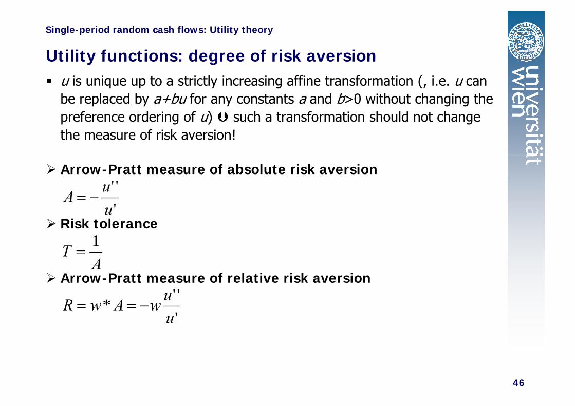
Single-period random cash flows: Utility theory
Utility functions: degree of risk aversionu is unique up to a strictly increasing affine transformation (, i.e. u can be replaced by a+bu for any constants a and b>0 without changing the preference ordering of u) such a transformation should not change the measure of risk aversion!
Arrow-Pratt measure of absolute risk aversion''uA −=
Risk tolerance'u
T 1=
Arrow-Pratt measure of relative risk aversionA
T =
''u'
*uuwAwR −==
46

Some utility functions
Single-period random cash flows: Utility theory
Some utility functionsPower utility 11
,)(−−
⎟⎟⎞
⎜⎜⎛
==γ wAwwu
Quadratic utility (special case of power utility: for = -1 )11
,1
)( ⎟⎟⎠
⎜⎜⎝− γγ
Awu
Negative exponential utility
( )w
Awforwwu−
=<−−=α
αα 1,,21)( 2
Logarithmic utility
ααα =>−= − Aforewu w ,0,)(
g y
( )w
Awforwwu+
=<−+=α
αα 1,,ln)(
All these utility functions are strictly increasing and strictly concave!
47

Expected utility and expected value criterion
Single-period random cash flows: Utility theory
Expected utility and expected value criterion
Obviously the expected value criterion can be reconciled with the expected utility approach by using a linear utilitywith the expected utility approach by using a linear utility function!
( ) wwu =( )
( )[ ] ( ) i
n
iii
n
ii wpwupwuE ∑∑ ==
11Recall that a linear utility function is equivalent to assuming risk neutrality.
h k l ( l l f ) h d
ii == 11
Thus, given risk neutrality (i.e. a linear utility function) the expected utility criterion reduces to the expected value criterion.
48

Expected utility and mean-variance criterion
Single-period random cash flows: Utility theory
Expected utility and mean variance criterion
The mean-variance criterion used in the Markowitz model can be reconciled with the expected utility approach incan be reconciled with the expected utility approach in either of two ways
using a quadratic utility function, org q y ,
assuming normal returns.
Quadratic utility functionUtility reaches a maximum at some wealth level and then declines.
As your wealth level increases, your willingness to take on risk decreases.
Normal returnsRecall that empirical results reveal that returns aren’t normal
49
distributed!


![[WorldBank] Qualitative Data](https://static.fdocuments.net/doc/165x107/577c7b911a28abe05497f7cb/worldbank-qualitative-data.jpg)