
Principles of Computer System Design - MIT … · Principles of Computer System Design An...
142
Principles of Computer System Design An Introduction Chapter 7 The Network as a System and as a System Component Jerome H. Saltzer M. Frans Kaashoek Massachusetts Institute of Technology Version 5.0 Saltzer & Kaashoek Ch. 7, p. i June 24, 2009 12:19 am
Transcript of Principles of Computer System Design - MIT … · Principles of Computer System Design An...
Principles of Computer System Design
An Introduction
Chapter 7 The Network as a System and as a System Component
Jerome H. Saltzer
M. Frans Kaashoek
Massachusetts Institute of Technology
Version 5.0
Saltzer & Kaashoek Ch. 7, p. i June 24, 2009 12:19 am
Copyright © 2009 by Jerome H. Saltzer and M. Frans Kaashoek. Some Rights Reserved.
This work is licensed under a Creative Commons Attribution-Noncommercial-Share Alike 3.0 United States License. For more information on what this license means, visit http://creativecommons.org/licenses/by-nc-sa/3.0/us/
Designations used by companies to distinguish their products are often claimed as trademarks or registered trademarks. In all instances in which the authors are aware of a claim, the product names appear in initial capital or all capital letters. All trademarks that appear or are otherwise referred to in this work belong to their respective owners.
Suggestions, Comments, Corrections, and Requests to waive license restrictions: Please send correspondence by electronic mail to:
Saltzer & Kaashoek Ch. 7, p. ii June 24, 2009 12:19 am

CHAPTER
The Network as a System and as a System 7Component
CHAPTER CONTENTS Overview..........................................................................................7–2 7.1 Interesting Properties of Networks ...........................................7–3
7.1.1 Isochronous and Asynchronous Multiplexing ............................ 7–5 7.1.2 Packet Forwarding; Delay ...................................................... 7–9 7.1.3 Buffer Overflow and Discarded Packets ................................. 7–12 7.1.4 Duplicate Packets and Duplicate Suppression ......................... 7–15 7.1.5 Damaged Packets and Broken Links ...................................... 7–18 7.1.6 Reordered Delivery ............................................................. 7–19 7.1.7 Summary of Interesting Properties and the Best-Effort Contract 7–20
7.2 Getting Organized: Layers.......................................................7–20 7.2.1 Layers .............................................................................. 7–23 7.2.2 The Link Layer ................................................................... 7–25 7.2.3 The Network Layer ............................................................. 7–27 7.2.4 The End-to-End Layer ......................................................... 7–28 7.2.5 Additional Layers and the End-to-End Argument ..................... 7–30 7.2.6 Mapped and Recursive Applications of the Layered Model ........ 7–32
7.3 The Link Layer.........................................................................7–34 7.3.1 Transmitting Digital Data in an Analog World ......................... 7–34 7.3.2 Framing Frames ................................................................. 7–38 7.3.3 Error Handling ................................................................... 7–40 7.3.4 The Link Layer Interface: Link Protocols and Multiplexing ........ 7–41 7.3.5 Link Properties .................................................................. 7–44
7.4 The Network Layer ..................................................................7–46 7.4.1 Addressing Interface .......................................................... 7–46 7.4.2 Managing the Forwarding Table: Routing ............................... 7–48 7.4.3 Hierarchical Address Assignment and Hierarchical Routing ....... 7–56 7.4.4 Reporting Network Layer Errors ........................................... 7–59 7.4.5 Network Address Translation (An Idea That Almost Works) ...... 7–61
7.5 The End-to-End Layer..............................................................7–62 7.5.1 Transport Protocols and Protocol Multiplexing ......................... 7–63 7.5.2 Assurance of At-Least-Once Delivery; the Role of Timers ......... 7–67 7.5.3 Assurance of At-Most-Once Delivery: Duplicate Suppression .... 7–71 7–1
Saltzer & Kaashoek Ch. 7, p. 1 June 25, 2009 8:22 am
7–2 CHAPTER 7 The Network as a System and as a System Component
7.5.4 Division into Segments and Reassembly of Long Messages ...... 7–73 7.5.5 Assurance of Data Integrity ................................................. 7–73 7.5.6 End-to-End Performance: Overlapping and Flow Control .......... 7–75
7.5.6.1 Overlapping Transmissions ............................................ 7–75 7.5.6.2 Bottlenecks, Flow Control, and Fixed Windows ................. 7–77 7.5.6.3 Sliding Windows and Self-Pacing .................................... 7–79 7.5.6.4 Recovery of Lost Data Segments with Windows................ 7–81
7.5.7 Assurance of Stream Order, and Closing of Connections .......... 7–82 7.5.8 Assurance of Jitter Control .................................................. 7–84 7.5.9 Assurance of Authenticity and Privacy ................................... 7–85
7.6 A Network System Design Issue: Congestion Control..............7–86 7.6.1 Managing Shared Resources ................................................ 7–86 7.6.2 Resource Management in Networks ...................................... 7–89 7.6.3 Cross-layer Cooperation: Feedback ....................................... 7–91 7.6.4 Cross-layer Cooperation: Control ......................................... 7–93 7.6.5 Other Ways of Controlling Congestion in Networks .................. 7–94 7.6.6 Delay Revisited .................................................................. 7–98
7.7 Wrapping up Networks............................................................7–99 7.8 Case Study: Mapping the Internet to the Ethernet ................7–100
7.8.1 A Brief Overview of Ethernet ...............................................7–100 7.8.2 Broadcast Aspects of Ethernet ............................................7–101 7.8.3 Layer Mapping: Attaching Ethernet to a Forwarding Network ...7–103 7.8.4 The Address Resolution Protocol ..........................................7–105
7.9 War Stories: Surprises in Protocol Design .............................7–107 7.9.1 Fixed Timers Lead to Congestion Collapse in NFS ..................7–107 7.9.2 Autonet Broadcast Storms ..................................................7–108 7.9.3 Emergent Phase Synchronization of Periodic Protocols ............7–108 7.9.4 Wisconsin Time Server Meltdown ........................................7–109
Exercises......................................................................................7–111 Glossary for Chapter 7 .................................................................7–125 Index of Chapter 7 .......................................................................7–135
Last chapter page 7–139
Overview Almost every computer system includes one or more communication links, and these communication links are usually organized to form a network, which can be loosely defined as a communication system that interconnects several entities. The basic abstraction remains SEND (message). and RECEIVE (message), so we can view a network as an elaboration of a communication link. Networks have several interesting properties— interface style, interface timing, latency, failure modes, and parameter ranges—that require careful design attention. Although many of these properties appear in latent form
Saltzer & Kaashoek Ch. 7, p. 2 June 25, 2009 8:22 am
7.1 Interesting Properties of Networks 7–3
in other system components, they become important or even dominate when the design includes communication.
Our study of networks begins, in Section 7.1, by identifying and investigating the interesting properties just mentioned, as well as methods of coping with those properties. Section 7.2 describes a three-layer reference model for a data communication network that is based on a best-effort contract, and Sections 7.3, 7.4, and 7.5 then explore more carefully a number of implementation issues and techniques for each of the three layers. Finally, Section 7.6 examines the problem of controlling network congestion.
A data communication network is an interesting example of a system itself. Most network designs make extensive use of layering as a modularization technique. Networks also provide in-depth examples of the issues involved in naming objects, in achieving fault tolerance, and in protecting information. (This chapter mentions fault tolerance and protection only in passing. Later chapters will return to these topics in proper depth.)
In addition to layering, this chapter identifies several techniques that have wide applicability both within computer networks and elsewhere in networked computer systems—framing, multiplexing, exponential backoff, best-effort contracts, latency masking, error control, and the end-to-end argument. A glance at the glossary will show that the chapter defines a large number of concepts. A particular network design is not likely to require them all, and in some contexts some of the ideas would be overkill. The engineering of a network as a system component requires trade-offs and careful judgement.
It is easy to be diverted into an in-depth study of networks because they are a fascinating topic in their own right. However, we will limit our exploration to their uses as system components and as a case study of system issues. If this treatment sparks a deeper interest in the topic, the Suggestions for Further Reading at the end of this book include several good books and papers that provide wide-ranging treatments of all aspects of networks.
7.1 Interesting Properties of Networks The design of communication networks is dominated by three intertwined considerations: (1) a trio of fundamental physical properties, (2) the mechanics of sharing, and (3) a remarkably wide range of parameter values.
The first dominating consideration is the trio of fundamental physical properties:
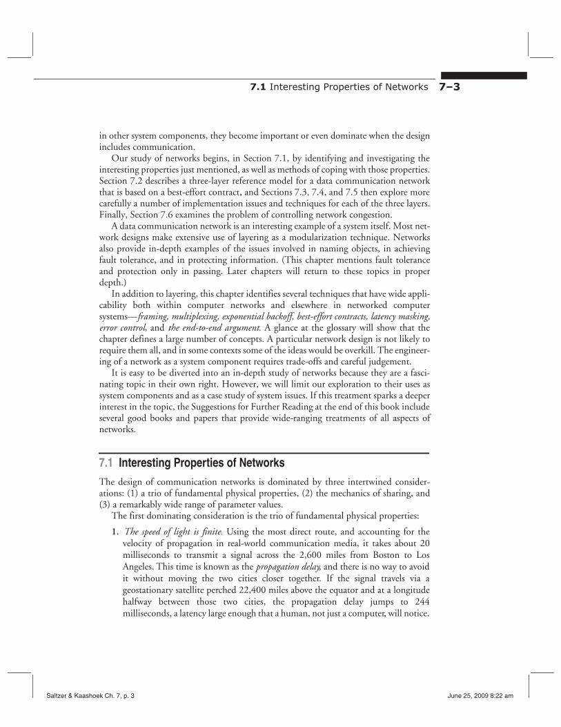
1. The speed of light is finite. Using the most direct route, and accounting for the velocity of propagation in real-world communication media, it takes about 20 milliseconds to transmit a signal across the 2,600 miles from Boston to Los Angeles. This time is known as the propagation delay, and there is no way to avoid it without moving the two cities closer together. If the signal travels via a geostationary satellite perched 22,400 miles above the equator and at a longitude halfway between those two cities, the propagation delay jumps to 244 milliseconds, a latency large enough that a human, not just a computer, will notice.
Saltzer & Kaashoek Ch. 7, p. 3 June 25, 2009 8:22 am

7–4 CHAPTER 7 The Network as a System and as a System Component
But communication between two computers in the same room may have a propagation delay of only 10 nanoseconds. That shorter latency makes some things easier to do, but the important implication is that network systems may have to accommodate a range of delay that spans seven orders of magnitude.
2. Communication environments are hostile. Computers are usually constructed of incredibly reliable components, and they are usually operated in relatively benign environments. But communication is carried out using wires, glass fibers, or radio signals that must traverse far more hostile environments ranging from under the floor to deep in the ocean. These environments endanger communication. Threats range from a burst of noise that wipes out individual bits to careless backhoe operators who sever cables that can require days to repair.
3. Communication media have limited bandwidth. Every transmission medium has a maximum rate at which one can transmit distinct signals. This maximum rate is determined by its physical properties, such as the distance between transmitter and receiver and the attenuation characteristics of the medium. Signals can be multilevel, not just binary, so the data rate can be greater than the signaling rate. However, noise limits the ability of a receiver to distinguish one signal level from another. The combination of limited signaling rate, finite signal power, and the existence of noise limits the rate at which data can be sent over a communication link.* Different network links may thus have radically different data rates, ranging from a few kilobits per second over a long-distance telephone line to several tens of gigabits per second over an optical fiber. Available data rate thus represents a second network parameter that may range over seven orders of magnitude.
The second dominating consideration of communications networks is that they are nearly always shared. Sharing arises for two distinct reasons.
1. Any-to-any connection. Any communication system that connects more than two things intrinsically involves an element of sharing. If you have three computers, you usually discover quickly that there are times when you want to communicate between any pair. You can start by building a separate communication path between each pair, but this approach runs out of steam quickly because the number of paths required grows with the square of the number of communicating entities. Even in a small network, a shared communication system is usually much more practical—it is more economical and it is easier to manage. When the number of entities that need to communicate begins to grow, as suggested in Figure 7.1, there is little choice. A closely related observation is that networks may connect three entities or 300 million entities. The number of connected entities is
* The formula that relates signaling rate, signal power, noise level, and maximum data rate, known as Shannon’s capacity theorem, appears on page 7–37.
Saltzer & Kaashoek Ch. 7, p. 4 June 25, 2009 8:22 am

7.1 Interesting Properties of Networks 7–5
thus a third network parameter with a wide range, in this case covering eight orders of magnitude.
2. Sharing of communication costs. Some parts of a communication system follow the same technological trends as do processors, memory, and disk: things made of silicon chips seem to fall in price every year. Other parts, such as digging up streets to lay wire or fiber, launching a satellite, or bidding to displace an existing radio-based service, are not getting any cheaper. Worse, when communication links leave a building, they require right-of-way, which usually subjects them to some form of regulation. Regulation operates on a majestic time scale, with procedures that involve courts and attorneys, legislative action, long-term policies, political pressures, and expediency. These procedures can eventually produce useful results, but on time scales measured in decades, whereas technological change makes new things feasible every year. This incommensurate rate of change means that communication costs rarely fall as fast as technology would permit, so sharing of those costs between otherwise independent users persists even in situations where the technology might allow them to avoid it.
The third dominating consideration of network design is the wide range of parameter values. We have already seen that propagation times, data rates, and the number of communicating computers can each vary by seven or more orders of magnitude. There is a fourth such wide-ranging parameter: a single computer may at different times present a network with widely differing loads, ranging from transmitting a file at 30 megabytes per second to interactive typing at a rate of one byte per second.
These three considerations, unyielding physical limits, sharing of facilities, and existence of four different parameters that can each range over seven or more orders of magnitude, intrude on every level of network design, and even carefully thought-out modularity cannot completely mask them. As a result, systems that use networks as a component must take them into account.
7.1.1 Isochronous and Asynchronous Multiplexing
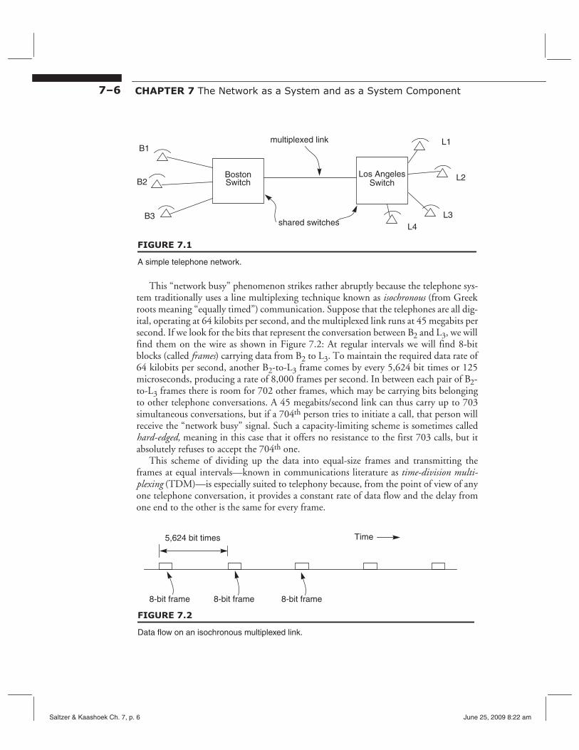
Sharing has significant consequences. Consider the simplified (and gradually becoming obsolescent) telephone network of Figure 7.1, which allows telephones in Boston to talk with telephones in Los Angeles: There are three shared components in this picture: a switch in Boston, a switch in Los Angeles, and an electrical circuit acting as a communication link between the two switches. The communication link is multiplexed, which means simply that it is used for several different communications at the same time. Let’s focus on the multiplexed link. Suppose that there is an earthquake in Los Angeles, and many people in Boston simultaneously try to call their relatives in Los Angeles to find out what happened. The multiplexed link has a limited capacity, and at some point the next caller will be told the “network is busy.” (In the U.S. telephone network this event is usually signaled with “fast busy,” a series of beeps repeated at twice the speed of a usual busy signal.)
Saltzer & Kaashoek Ch. 7, p. 5 June 25, 2009 8:22 am
7–6 CHAPTER 7 The Network as a System and as a System Component
Boston Switch
Los Angeles Switch
multiplexed link
shared switches
B1
B2
B3
L1
L2
L3 L4
FIGURE 7.1
A simple telephone network.
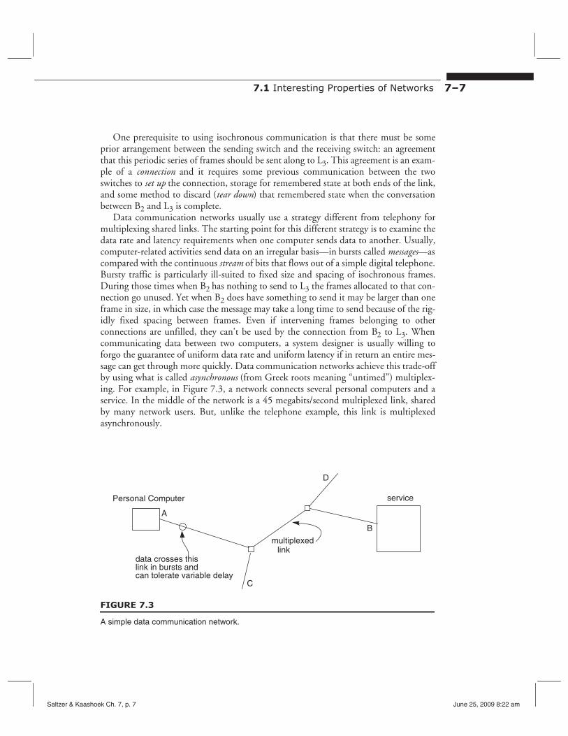
This “network busy” phenomenon strikes rather abruptly because the telephone system traditionally uses a line multiplexing technique known as isochronous (from Greek roots meaning “equally timed”) communication. Suppose that the telephones are all digital, operating at 64 kilobits per second, and the multiplexed link runs at 45 megabits per second. If we look for the bits that represent the conversation between B2 and L3, we will find them on the wire as shown in Figure 7.2: At regular intervals we will find 8-bit blocks (called frames) carrying data from B2 to L3. To maintain the required data rate of 64 kilobits per second, another B2-to-L3 frame comes by every 5,624 bit times or 125 microseconds, producing a rate of 8,000 frames per second. In between each pair of B2to-L3 frames there is room for 702 other frames, which may be carrying bits belonging to other telephone conversations. A 45 megabits/second link can thus carry up to 703 simultaneous conversations, but if a 704th person tries to initiate a call, that person will receive the “network busy” signal. Such a capacity-limiting scheme is sometimes called hard-edged, meaning in this case that it offers no resistance to the first 703 calls, but it absolutely refuses to accept the 704th one.
This scheme of dividing up the data into equal-size frames and transmitting the frames at equal intervals—known in communications literature as time-division multiplexing (TDM)—is especially suited to telephony because, from the point of view of any one telephone conversation, it provides a constant rate of data flow and the delay from one end to the other is the same for every frame.
Time5,624 bit times
8-bit frame 8-bit frame 8-bit frame
FIGURE 7.2
Data flow on an isochronous multiplexed link.
Saltzer & Kaashoek Ch. 7, p. 6 June 25, 2009 8:22 am
7.1 Interesting Properties of Networks 7–7
One prerequisite to using isochronous communication is that there must be some prior arrangement between the sending switch and the receiving switch: an agreement that this periodic series of frames should be sent along to L3. This agreement is an example of a connection and it requires some previous communication between the two switches to set up the connection, storage for remembered state at both ends of the link, and some method to discard (tear down) that remembered state when the conversation between B2 and L3 is complete.
Data communication networks usually use a strategy different from telephony for multiplexing shared links. The starting point for this different strategy is to examine the data rate and latency requirements when one computer sends data to another. Usually, computer-related activities send data on an irregular basis—in bursts called messages—as compared with the continuous stream of bits that flows out of a simple digital telephone. Bursty traffic is particularly ill-suited to fixed size and spacing of isochronous frames. During those times when B2 has nothing to send to L3 the frames allocated to that connection go unused. Yet when B2 does have something to send it may be larger than one frame in size, in which case the message may take a long time to send because of the rigidly fixed spacing between frames. Even if intervening frames belonging to other connections are unfilled, they can’t be used by the connection from B2 to L3. When communicating data between two computers, a system designer is usually willing to forgo the guarantee of uniform data rate and uniform latency if in return an entire message can get through more quickly. Data communication networks achieve this trade-off by using what is called asynchronous (from Greek roots meaning “untimed”) multiplexing. For example, in Figure 7.3, a network connects several personal computers and a service. In the middle of the network is a 45 megabits/second multiplexed link, shared by many network users. But, unlike the telephone example, this link is multiplexed asynchronously.
Personal Computer service
multiplexed link
data crosses this link in bursts and can tolerate variable delay
A
B
C
D
FIGURE 7.3
A simple data communication network.
Saltzer & Kaashoek Ch. 7, p. 7 June 25, 2009 8:22 am
7–8 CHAPTER 7 The Network as a System and as a System Component
frame
Time
B D
Guidance 4000 bits 750 bits information
FIGURE 7.4
Data flow on an asynchronous multiplexed link.
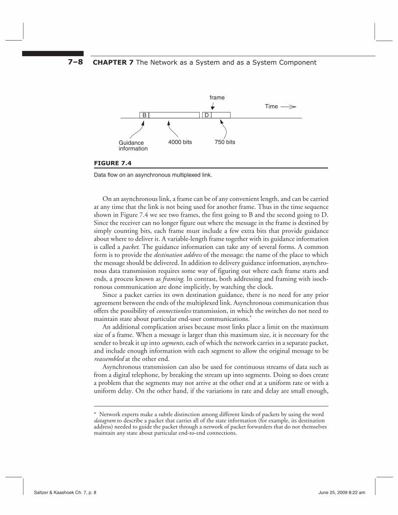
On an asynchronous link, a frame can be of any convenient length, and can be carried at any time that the link is not being used for another frame. Thus in the time sequence shown in Figure 7.4 we see two frames, the first going to B and the second going to D. Since the receiver can no longer figure out where the message in the frame is destined by simply counting bits, each frame must include a few extra bits that provide guidance about where to deliver it. A variable-length frame together with its guidance information is called a packet. The guidance information can take any of several forms. A common form is to provide the destination address of the message: the name of the place to which the message should be delivered. In addition to delivery guidance information, asynchronous data transmission requires some way of figuring out where each frame starts and ends, a process known as framing. In contrast, both addressing and framing with isochronous communication are done implicitly, by watching the clock.
Since a packet carries its own destination guidance, there is no need for any prior agreement between the ends of the multiplexed link. Asynchronous communication thus offers the possibility of connectionless transmission, in which the switches do not need to maintain state about particular end-user communications.*
An additional complication arises because most links place a limit on the maximum size of a frame. When a message is larger than this maximum size, it is necessary for the sender to break it up into segments, each of which the network carries in a separate packet, and include enough information with each segment to allow the original message to be reassembled at the other end.
Asynchronous transmission can also be used for continuous streams of data such as from a digital telephone, by breaking the stream up into segments. Doing so does create a problem that the segments may not arrive at the other end at a uniform rate or with a uniform delay. On the other hand, if the variations in rate and delay are small enough,
* Network experts make a subtle distinction among different kinds of packets by using the word datagram to describe a packet that carries all of the state information (for example, its destination address) needed to guide the packet through a network of packet forwarders that do not themselves maintain any state about particular end-to-end connections.
Saltzer & Kaashoek Ch. 7, p. 8 June 25, 2009 8:22 am
7.1 Interesting Properties of Networks 7–9
Packet Switch Packet
Switch
Packet Switch
Packet Switch
Service at network
Workstation
packet
1
2 3at network attachment
attachment point B
A
B
B
point A
FIGURE 7.5
A packet forwarding network.
or the application can tolerate occasional missing segments of data, the method is still effective. In the case of telephony, the technique is called “packet voice” and it is gradually replacing many parts of the traditional isochronous voice network.
7.1.2 Packet Forwarding; Delay
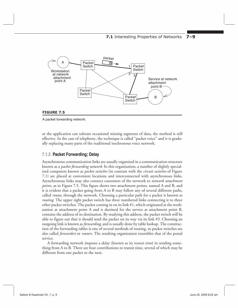
Asynchronous communication links are usually organized in a communication structure known as a packet forwarding network. In this organization, a number of slightly specialized computers known as packet switches (in contrast with the circuit switches of Figure 7.1) are placed at convenient locations and interconnected with asynchronous links. Asynchronous links may also connect customers of the network to network attachment points, as in Figure 7.5. This figure shows two attachment points, named A and B, and it is evident that a packet going from A to B may follow any of several different paths, called routes, through the network. Choosing a particular path for a packet is known as routing. The upper right packet switch has three numbered links connecting it to three other packet switches. The packet coming in on its link #1, which originated at the workstation at attachment point A and is destined for the service at attachment point B, contains the address of its destination. By studying this address, the packet switch will be able to figure out that it should send the packet on its way via its link #3. Choosing an outgoing link is known as forwarding, and is usually done by table lookup. The construction of the forwarding tables is one of several methods of routing, so packet switches are also called forwarders or routers. The resulting organization resembles that of the postal service.
A forwarding network imposes a delay (known as its transit time) in sending something from A to B. There are four contributions to transit time, several of which may be different from one packet to the next.
Saltzer & Kaashoek Ch. 7, p. 9 June 25, 2009 8:22 am

7–10 CHAPTER 7 The Network as a System and as a System Component
1. Propagation delay. The time required for the signal to travel across a link is determined by the speed of light in the transmission medium connecting the packet switches and the physical distance the signals travel. Although it does vary slightly with temperature, from the point of view of a network designer propagation delay for any given link can be considered constant. (Propagation delay also applies to the isochronous network.)
2. Transmission delay. Since the frame that carries the packet may be long or short, the time required to send the frame at one switch—and receive it at the next switch—depends on the data rate of the link and the length of the frame. This time is known as transmission delay. Although some packet switches are clever enough to begin sending a packet out before completely receiving it (a trick known as cut-through), error recovery is simpler if the switch does not forward a packet until the entire packet is present and has passed some validity checks. Each time the packet is transmitted over another link, there is another transmission delay. A packet going from A to B via the dark links in Figure 7.5 will thus be subject to four transmission delays, one when A sends it to the first packet switch, one at each forwarding step, and finally one to transmit it to B.
3. Processing delay. Each packet switch will have to examine the guidance information in the packet to decide to which outgoing link to send it. The time required to figure this out, together with any other work performed on the packet, such as calculating a checksum (see Sidebar 7.1) to allow error detection or copying it to an output buffer that is somewhere else in memory, is known as processing delay.
Sidebar 7.1: Error detection, checksums, and witnesses A checksum on a block of data is a stylized kind of error-detection code in which redundant error-detecting information, rather than being encoded into the data itself (as Chapter 8[on-line] will explain), is placed in a separate field. A typical simple checksum algorithm breaks the data block up into k-bit chunks and performs an exclusive OR on the chunks to produce a k-bit result. (When k = 1, this procedure is called a parity check.) That simple k-bit checksum would catch any one-bit error, but it would miss some two-bit errors, and it would not detect that two chunks of the block have been interchanged. Much more sophisticated checksum algorithms have been devised that can detect multiple-bit errors or that are good at detecting particular kinds of expected errors. As will be seen in Chapter 11[on-line], by using cryptographic techniques it is possible to construct a high-quality checksum with the property that it can detect all changes—even changes that have been intentionally introduced by a malefactor—with near certainty. Such a checksum is called a witness, or fingerprint and is useful for ensuring long-term integrity of stored data.The trade-off is that more elaborate checksums usually require more time to calculate and thus add to processing delay. For that reason, communication systems typically use the simplest checksum algorithm that has a reasonable chance of detecting the expected errors.
Saltzer & Kaashoek Ch. 7, p. 10 June 25, 2009 8:22 am
7.1 Interesting Properties of Networks 7–11
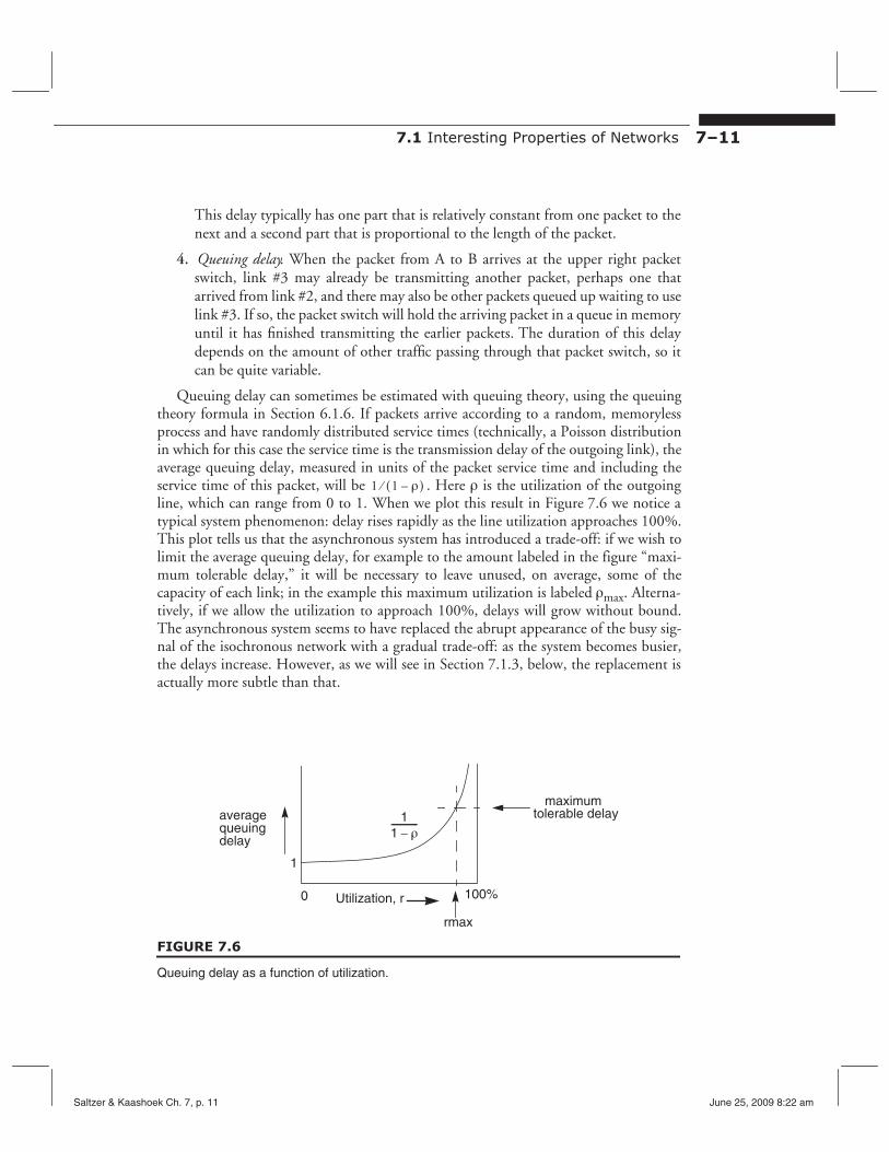
This delay typically has one part that is relatively constant from one packet to the next and a second part that is proportional to the length of the packet.
4. Queuing delay. When the packet from A to B arrives at the upper right packet switch, link #3 may already be transmitting another packet, perhaps one that arrived from link #2, and there may also be other packets queued up waiting to use link #3. If so, the packet switch will hold the arriving packet in a queue in memory until it has finished transmitting the earlier packets. The duration of this delay depends on the amount of other traffic passing through that packet switch, so it can be quite variable.
Queuing delay can sometimes be estimated with queuing theory, using the queuing theory formula in Section 6.1.6. If packets arrive according to a random, memoryless process and have randomly distributed service times (technically, a Poisson distribution in which for this case the service time is the transmission delay of the outgoing link), the average queuing delay, measured in units of the packet service time and including the service time of this packet, will be 1 1 – ρ) . Here ρ is the utilization of the outgoing⁄ ( line, which can range from 0 to 1. When we plot this result in Figure 7.6 we notice a typical system phenomenon: delay rises rapidly as the line utilization approaches 100%. This plot tells us that the asynchronous system has introduced a trade-off: if we wish to limit the average queuing delay, for example to the amount labeled in the figure “maximum tolerable delay,” it will be necessary to leave unused, on average, some of the capacity of each link; in the example this maximum utilization is labeled ρmax. Alternatively, if we allow the utilization to approach 100%, delays will grow without bound. The asynchronous system seems to have replaced the abrupt appearance of the busy signal of the isochronous network with a gradual trade-off: as the system becomes busier, the delays increase. However, as we will see in Section 7.1.3, below, the replacement is actually more subtle than that.
average
1
1 1 ρ– ------------
tolerable delay queuing delay
maximum
0 Utilization, r 100%
FIGURE 7.6
rmax
Queuing delay as a function of utilization.
Saltzer & Kaashoek Ch. 7, p. 11 June 25, 2009 8:22 am

7–12 CHAPTER 7 The Network as a System and as a System Component
The formula and accompanying graph tell us only the average delay. If we try to load up a link so that its utilization is ρmax, the actual delay will exceed our tolerance threshold about as often as it is below that threshold. If we are serious about keeping the maximum delay almost always below a given value, we must prepare for occasional worse peaks by holding utilization below the level of ρmax suggested by the figure. If packets do not obey memoryless arrival statistics (for example, they arrive in long convoys, and all are the same, maximum size), the model no longer applies, and we need a better understanding of the arrival process before we can say anything about delays. This same utilization versus delay trade-off also applies to non-network components of a computer system that have queues, for example scheduling the processor or reading and writing a magnetic disk.
We have talked about queuing theory as if it might be useful in predicting the behavior of a network. It is not. In practice, network systems put a bound on link queuing delays by limiting the size of queues and by exerting control on arrivals. These mechanisms allow individual links to achieve high utilization levels, while shifting delays to other places in the network. The next section explains how, and it also explains just what happened to the isochronous network’s hard-edged busy signal. Later, in Section 7.6 of this chapter we will see how the delays can be shifted all the way back to the entry point of the network.
7.1.3 Buffer Overflow and Discarded Packets
Continuing for a moment to apply queuing theory, queuing has an implication: buffer space is needed to hold the queue of packets waiting for transmission. How large a buffer should the designer allocate? Under the memoryless arrival interval assumption, the average number of packets awaiting transmission (including the one currently being transmitted) is 1 1 – ρ) . As with queuing delay, that number is only the average—⁄ ( queuing theory tells us that the variance of the queue length is also 1 1 – ρ) . For a ρ of⁄ ( 0.8 the average queue length and the variance are both 5, so if one wishes to allow enough buffers to handle peaks that are, say, three standard deviations above the average, one must be prepared to buffer not only the 5 packets predicted as the average but also (3 × 5 ≅ 7) more, a total of 12 packets. Worse, in many real networks packets don’t actually arrive independently at random; they come in buffer-bursting batches.
At this point, we can imagine three quite different strategies for choosing a buffer size:
1. Plan for the worst case. Examine the network traffic carefully, figure out what the worst-case traffic situation will be, and allocate enough buffers to handle it.
2. Plan for the usual case and fight back. Based on a calculation such as the one above, choose a buffer size that will work most of the time, and if the buffers fill up send messages back through the network asking someone to stop sending.
3. Plan for the usual case and discard overflow. Again, choose a buffer size that will work most of the time, and ruthlessly discard packets when the buffers are full.
Saltzer & Kaashoek Ch. 7, p. 12 June 25, 2009 8:22 am

7.1 Interesting Properties of Networks 7–13
Let’s explore these three possibilities in turn. Buffer memory is usually low in cost, so planning for the worst case seems like an
attractive idea, but it is actually much harder than it sounds. For one thing, in a large network, it may be impossible to figure out what the worst case is—there just isn’t enough information available about what can happen. Even if one can estimate the worst case, the estimate may not be useful. Consider, for example, the Hypothetical Bank of Canada, which has 21,000 tellers scattered across the country. The branch at Moose Jaw, Saskatchewan, has one teller and usually is the target of only three transactions a day. Although it has never happened, and almost certainly never will, the worst case is that every one of the 20,999 other tellers simultaneously posts a withdrawal against a Moose Jaw account. Thus a worst-case design would require that there be enough buffers in the packet switch leading to Moose Jaw to handle 20,999 simultaneous messages. The problem with worst-case analysis is that the worst case can be many orders of magnitude larger than the average case, as well as extremely unlikely. Moreover, even if one decided to buy that large a buffer, the resulting queue to process all the transactions would be so long that many of the other tellers would give up in disgust and abort their transactions, so the large buffer wouldn’t really help.
This observation makes it sound attractive to choose a buffer size based on typical, rather than worst-case, loads. But then there is always going to be a chance that traffic will exceed the average for long enough to run out of buffer space. This situation is called congestion. What to do then?
One idea is to push back. If buffer space begins to run low, send a message back along an incoming link saying “please don’t send any more until you hear from me”. This message (called a quench request) may go to the packet switch at the other end of that link, or it may go all the way back to the original source that introduced the data into the network. Either way, pushing back is also harder than it sounds. If a packet switch is experiencing congestion, there is a good chance that the adjacent switch is also congested (if it is not already congested, it soon will be if it is told to stop sending data over the link to this switch), and sending an extra message is adding to the congestion. Worse, a set of packet switches configured in a cycle like that of Figure 7.5 can easily end up in a form of deadlock (called gridlock when it happens to automobile traffic), with all buffers filled and each switch waiting for the next switch to say that it is OK to start sending again.
One way to avoid deadlock among the packet switches is to send the quench request all the way back to the source. This method is hard too, for at least three reasons. First, it may not be clear to which source to send the quench. In our Moose Jaw example, there are 21,000 different sources, no one of which is, by itself, the cause of (nor capable of doing much about) the problem. Second, such a request may not have any effect because the source you choose to quench is no longer sending anyway. Again in our example, by the time the packet switch on the way to Moose Jaw detects the overload, all of the 21,000 tellers may have already sent their transaction requests, so asking them not to send anything else would accomplish nothing. Third, assuming that the quench message is itself forwarded back through the packet-switched network, it may run into congestion and be subject to queuing delays. The busier the network, the longer it will take to exert
Saltzer & Kaashoek Ch. 7, p. 13 June 25, 2009 8:22 am
7–14 CHAPTER 7 The Network as a System and as a System Component
control. We are proposing to create a feedback system with delay and should expect to see oscillations. Even if all the data is coming from one source, by the time the quench gets back and the source acts on it, the packets already in the pipeline may exceed the buffer capacity. Controlling congestion by quenching either the adjacent switch or the source is used in various special situations, but as a general technique it is currently an unsolved problem.
The remaining possibility is what most packet networks actually do in the face of congestion: when the buffers fill up, they start throwing packets away. This seems like a somewhat startling thing for a communication system to do because it will disrupt the communication, and eventually each discarded packet will have to be sent again, so the effort to send the packet this far will have been wasted. Nevertheless, this is an action that every packet switching network that is not configured for the worst case must be prepared to take.
Overflowing buffers and discarded packets lead to two remarkable consequences. First, the sender of a packet can interpret the lack of its acknowledgment as a sign that the network is congested, and can in turn reduce the rate at which it introduces new packets into the network. This idea, called automatic rate adaptation, is explored in depth in Section 7.6 of this chapter. The combination of discarded packets and automatic rate adaptation in turn produce the second consequence: simple theoretical models of network behavior based on standard queuing theory do not apply when a service may serve some requests and may discard others. Modeling of networks that have rate adaptation requires a much deeper understanding of the specific algorithms used not just by the network but also by network applications.
In the final analysis, the asynchronous network replaces the hard-edged blocking of the isochronous network with a variable transmission rate that depends on the instantaneous network load. Which scheme (asynchronous or isochronous) for dealing with overload is preferable depends on the application. For some applications it may be better to be told at the outset of a communications attempt to come back later, rather than to be allowed to start work only to encounter such variations in available capacity that it is hard to do anything useful. In other applications it may be more helpful to have some work done, slowly or at variable rates, rather than none at all.
The possibility that a network may actually discard packets to cope with congestion leads to a useful distinction between two kinds of forwarding networks. So far, we have been discussing what is usually described as a best-effort network, which, if it cannot dispatch a packet soon after receipt, may discard it. The alternative design is the guaranteed-delivery network (sometimes called a store-and-forward network, although that term is often applied to all forwarding networks), which takes heroic measures to avoid ever discarding payload data. Guaranteed delivery networks usually are designed to work with complete messages rather than packets. Typically, a guaranteed delivery network uses non-volatile storage such as a magnetic disk for buffering, so that it can handle large peaks of message load and can be confident that messages will not be lost even if there is a power failure or the forwarding computer crashes. Also, a guaranteed delivery network usually, when faced with the prospect of being completely unable to deliver a message
Saltzer & Kaashoek Ch. 7, p. 14 June 25, 2009 8:22 am
7.1 Interesting Properties of Networks 7–15
(perhaps because the intended recipient has vanished), explicitly returns the message to its originator along with an explanation of why delivery failed. Finally, in keeping with the spirit of not losing a message, a guaranteed delivery switch usually tracks individual messages carefully to make sure that none are lost or damaged during transmission, for example by a burst of noise. A switch of a best-effort network can be quite a bit simpler than a switch of a guaranteed-delivery network. Since the best-effort network may casually discard packets anyway, it does not need to make any special provisions for retransmitting damaged packets, for preserving packets in transit when the switch crashes and restarts, or for worrying about the case when the link to a destination node suddenly stops accepting data.
The best-effort network is said to provide a best-effort contract to its customers (this contract is defined more carefully in Section 7.1.7, below), rather than a guarantee of delivery. Of course, in the real world there are no absolute guarantees—the real distinction between the two designs is that there is intended to be a significant difference in the probability of undetected loss. When we examine network layering in Section 7.2 of this chapter, it will become apparent that these differences can be characterized another way: guaranteed-delivery networks are usually implemented in a higher network layer, best-effort networks in a lower network layer.
In these terms, the U.S. Postal Service operates a guaranteed delivery system for first-class mail, but a best-effort system for third-class (junk) mail, because postal regulations allow it to discard third-class mail that is misaddressed or when congestion gets out of hand. The Internet is organized as a best-effort system, but the Internet mechanisms for handling e-mail are designed as a guaranteed delivery system. The Western Union company has always prided itself on operating a true guaranteed-delivery system, to the extent that when it decommissions an office it normally disassembles the site completely in a search for misplaced telegrams. There is a (possibly apocryphal) tale that such a disassembly once discovered a 75-year-old telegram that had fallen behind a water pipe. The company promptly delivered it to the astonished heirs of the original addressee.
7.1.4 Duplicate Packets and Duplicate Suppression
As it turns out, discarded packets are not as much of a problem to the higher-level application as one might expect because when a client sends a request to a service, it is always possible that the service is not available, or the service crashed just after receiving the request. So unanswered requests are actually a routine occurrence, and many network protocols include some kind of timer expiration and resend mechanism to recover from such failures. The timing diagram of Figure 7.7* illustrates the situation, showing a first packet carrying a request, followed by a packet going the other way carrying the response to the first request. A has set a timer, indicated by a vertical line, but the arrival of response 1 before the expiration of the timer causes A to switch off the timer, indicated by the small X. The packet carrying the second request is lost in transit (as indicated by
* The conventions for representation of timing diagrams were described in Sidebar 4.2.
Saltzer & Kaashoek Ch. 7, p. 15 June 25, 2009 8:22 am

7–16 CHAPTER 7 The Network as a System and as a System Component
A B
send request, set timer
receive response, reset timer
send request, set timer
timer expires, resend request, set new timer
receive response, reset timer
FIGURE 7.7
time
X
request 1
response 1
request 2
request 2’
overloaded
response 2’
X
X
forwarder discards request packet.
Lost packet recovery.
the large X), perhaps having been damaged or discarded by an overloaded forwarder, the timer expires, and A resends request 2 in the packet labeled request 2’.
When a congested forwarder discards a packet, there are two important consequences. First, the client doesn’t receive a response as quickly as originally hoped because a timer expiration period has been added to the overall response time. This extra delay can have a significant impact on performance. Second, users of the network must be prepared for duplicate requests and responses. The reason lies in the recovery mechanism just described. Suppose a network packet switch gets overloaded and must discard a response packet, as in Figure 7.8. Client A can’t tell the difference between this case and the case of Figure 7.7, so it resends its request. The service sees this resent request as a duplicate. Suppose B does not realize this is a duplicate, does what is requested, and sends back a response. Client A receives the response and assumes that everything is OK. That may be a correct assumption, or it may not, depending on whether or not the first arrival of request 3 changed B’s state. If B is a spelling checker, it will probably give the same response to both copies of the request. But if B is a bank and the request is to transfer funds, doing the request twice would be a mistake. So detecting duplicates may or may not be important, depending on the particular application.
For another example, if for some reason the network delays pile up and exceed the resend timer expiration period, the client may resend a request even though the original
Saltzer & Kaashoek Ch. 7, p. 16 June 25, 2009 8:22 am

request 3
7.1 Interesting Properties of Networks 7–17
B send request,
set timer
A
resend request,set new timer
X overloaded forwarder timer expires, discards response 3
request 3’
response 3’ duplicate arrives at B B sends response 3’
receive response,reset timer X
FIGURE 7.8
ost packet recovery leading to duplicate request.
response is still in transit. Since B can’t tell any difference between this case and the previous one, it responds in the same way, by doing what is requested. But now A receives a duplicate response, as in Figure 7.9. Again, this duplicate may or may not matter to A, but at minimum A must take steps not to be confused by the arrival of a duplicate response.
What if the arrival of a request from A causes B to change state, as in the bank transfer example? If so, it is usually important to detect and suppress duplicates generated by the lost packet recovery mechanism. The general procedure to suppress duplicates has two components. The first component is hinted at by the request and response numbers used in the illustrations: each request includes a nonce, which is a unique identifier that will
BA
send request,set timer
timer expires, resend receive
response,reset timer
receive duplicate response
FIGURE 7.9
request 4
request 4’
response 4’
response 4
X
packet containing responsegets delayed
duplicate arrives at B B sends response 4’
Network delay combined with recovery leading to duplicate response.
Saltzer & Kaashoek Ch. 7, p. 17 June 25, 2009 8:22 am
7–18 CHAPTER 7 The Network as a System and as a System Component
never be reused by A when sending requests to B. The illustration uses monotonically increasing serial numbers as nonces, but any unique identifier will do. The second duplicate suppression component is that B must maintain a list of nonces on which it has taken action or is still working, and whenever a request arrives B should look through this list to see whether or not this apparently new request is actually a duplicate of one previously received. If it is a duplicate B must not perform the action requested. On the other hand, B should not simply ignore the request, either, because the reason for the duplicate may be that A never received B’s response. So B needs some way of reconstructing and resending that previous response. The simplest way of doing this is usually for B to add to its list of previously handled nonces a copy of the corresponding responses so that it can easily resend them. Thus in Figure 7.9, the last action of B should be replaced with “B resends response 4”.
In some network designs, A may even receive duplicate responses to a single, unrepeated request. The reason is that a forwarding link deep inside the network may be using a timer expiration and resend protocol similar to the one above. For this reason, most protocols that are concerned about duplicate suppression include a copy of the nonce in the response, and the originator, A, maintains a list of nonces used in its outstanding requests. When a response comes back, A can check for the nonce in the list and delete that list entry or, if there is no list entry, assume it is a duplicate of a previously received response and ignore it.
The procedure we have just described allows A to keep its list of nonces short, but B might have to maintain an ever-growing list of nonces and responses to be certain that it never accidentally processes a request twice. A related problem concerns what happens if either participant crashes and restarts, losing its volatile memory, which is probably where it is keeping its list of nonces. Refinements to cope with these problems will be explored in detail when we revisit the topic of duplicate suppression on page 7–71 of this chapter.
Ensuring suppression of duplicates is a significant complication so, if possible, it is wise to design the service and its protocol in such a way that suppression is not required. Recall that the reason that duplicate suppression became important was that a request changed the state of the service. It is often possible to design a service interface so that it is idempotent, which for a network request means that repeating the same request or sequence of requests several times has the same effect as doing it just once. This design approach is explored in depth in the discussion of atomicity and error recovery in Chapter 9[on-line].
7.1.5 Damaged Packets and Broken Links
At the beginning of the chapter we noted that noise is one of the fundamental considerations that dominates the design of data communication. Data can be damaged during transmission, during transit through a switch, or in the memory of a forwarding node. Noise, transmission errors, and techniques for detecting and correcting errors are fascinating topics in their own right, explored in some depth in Chapter 8[on-line]. As a
Saltzer & Kaashoek Ch. 7, p. 18 June 25, 2009 8:22 am
7.1 Interesting Properties of Networks 7–19
general rule it is possible to sub-contract this area to a specialist in the theory of error detection and correction, with one requirement in the contract: when we receive data, we want to know whether or not it is correct. That is, we require that a reliable error detection mechanism be part of any underlying data transmission system. Section 7.3.3 of this chapter expands a bit on this error detection requirement.
Once we have contracted for data transmission with an error detection mechanism in which we have confidence, intermediate packet switches can then handle noise-damaged packets by simply discarding them. This approach changes the noise problem into one for which there is already a recovery procedure. Put another way, this approach transforms data loss into performance degradation.
Finally, because transmission links traverse hostile environments and must be considered fragile, a packet network usually has multiple interconnection paths, as in Figure 7.5. Links can go down while transmitting a frame; they may stay down briefly, e.g. because of a power interruption, or for long periods of time while waiting for someone to dig up a street or launch a replacement satellite. Flexibility in routing is an important property of a network of any size. We will return to the implications of broken links in the discussion of the network layer, in Section 7.4 of this chapter.
7.1.6 Reordered Delivery
When a packet-forwarding network has an interconnection topology like that of Figure 7.5, in which there is more than one path that a packet can follow from A to B, there is a possibility that a series of packets departing from A in sequential order may arrive at B in a different order. Some networks take special precautions to avoid this possibility by forcing all packets between the same two points to take the same path or by delaying delivery at the destination until all earlier packets have arrived. Both of these techniques introduce additional delay, and there are applications for which reducing delay is more important than receiving the segments of a message in the order in which they were transmitted.
Recalling that a message may have been divided into segments, the possibility of reordered delivery means that reassembly of the original message requires close attention. We have here a model of communication much like when a friend is touring on holiday by car, stopping each night in a different motel, and sending a motel postcard with an account of the day’s adventures. Whenever a day’s story doesn’t fit on one card, your friend uses two or three postcards, as necessary. The Post Office may deliver these cards to you in almost any order, and something on the postcard—probably the date—will be needed to enable you to read them in the proper order. Even when two cards are mailed at the same time from the same motel (as indicated by the motel photograph on the front) the Post Office may deliver them to you on different days, so there must be further information on the postcard to allow you to realize that sender broke the original message into segments and you may need to wait for the next delivery before starting to read.
Saltzer & Kaashoek Ch. 7, p. 19 June 25, 2009 8:22 am
7–20 CHAPTER 7 The Network as a System and as a System Component
7.1.7 Summary of Interesting Properties and the Best-Effort Contract
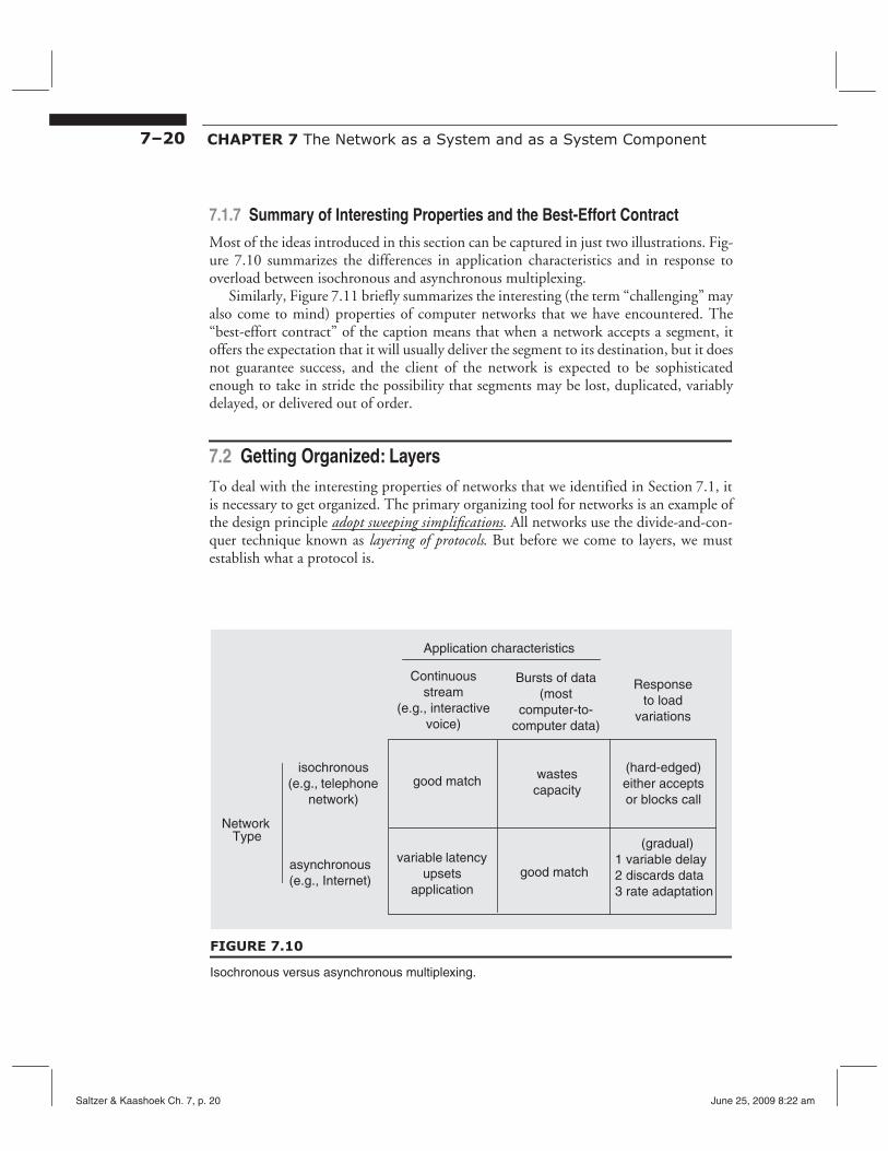
Most of the ideas introduced in this section can be captured in just two illustrations. Figure 7.10 summarizes the differences in application characteristics and in response to overload between isochronous and asynchronous multiplexing.
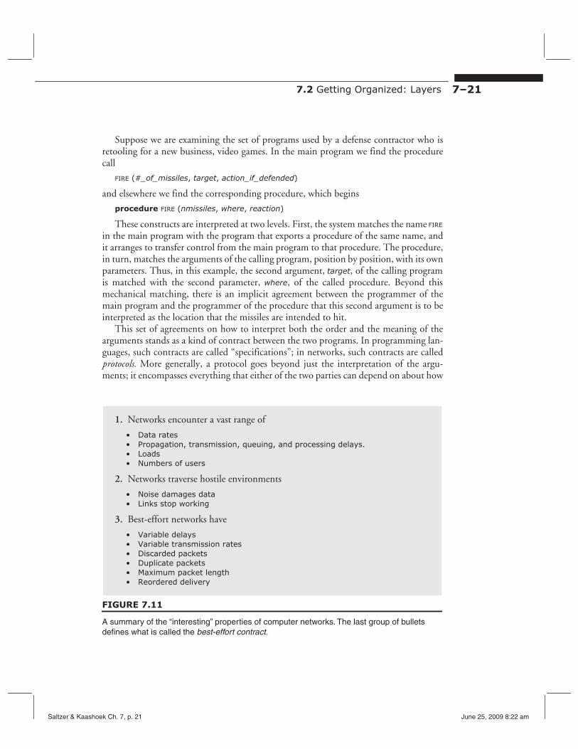
Similarly, Figure 7.11 briefly summarizes the interesting (the term “challenging” may also come to mind) properties of computer networks that we have encountered. The “best-effort contract” of the caption means that when a network accepts a segment, it offers the expectation that it will usually deliver the segment to its destination, but it does not guarantee success, and the client of the network is expected to be sophisticated enough to take in stride the possibility that segments may be lost, duplicated, variably delayed, or delivered out of order.
7.2 Getting Organized: Layers To deal with the interesting properties of networks that we identified in Section 7.1, it is necessary to get organized. The primary organizing tool for networks is an example of the design principle adopt sweeping simplifications. All networks use the divide-and-conquer technique known as layering of protocols. But before we come to layers, we must establish what a protocol is.
Application characteristics
Continuous Bursts of data stream (most
(e.g., interactive computer-tovoice)
isochronous (e.g., telephone good match
network)
Network Type
variable latencyasynchronous (e.g., Internet) upsets
application
FIGURE 7.10
computer data)
wastes capacity
good match
Response to load
variations
(hard-edged) either accepts or blocks call
(gradual) 1 variable delay 2 discards data 3 rate adaptation
Isochronous versus asynchronous multiplexing.
Saltzer & Kaashoek Ch. 7, p. 20 June 25, 2009 8:22 am
7.2 Getting Organized: Layers 7–21
Suppose we are examining the set of programs used by a defense contractor who is retooling for a new business, video games. In the main program we find the procedure call
FIRE (#_of_missiles, target, action_if_defended)
and elsewhere we find the corresponding procedure, which begins
procedure FIRE (nmissiles, where, reaction)
These constructs are interpreted at two levels. First, the system matches the name FIRE
in the main program with the program that exports a procedure of the same name, and it arranges to transfer control from the main program to that procedure. The procedure, in turn, matches the arguments of the calling program, position by position, with its own parameters. Thus, in this example, the second argument, target, of the calling program is matched with the second parameter, where, of the called procedure. Beyond this mechanical matching, there is an implicit agreement between the programmer of the main program and the programmer of the procedure that this second argument is to be interpreted as the location that the missiles are intended to hit.
This set of agreements on how to interpret both the order and the meaning of the arguments stands as a kind of contract between the two programs. In programming languages, such contracts are called “specifications”; in networks, such contracts are called protocols. More generally, a protocol goes beyond just the interpretation of the arguments; it encompasses everything that either of the two parties can depend on about how
FIGURE 7.11
1. Networks encounter a vast range of
• Data rates • Propagation, transmission, queuing, and processing delays. • Loads • Numbers of users
2. Networks traverse hostile environments
• Noise damages data • Links stop working
3. Best-effort networks have
• Variable delays • Variable transmission rates • Discarded packets • Duplicate packets • Maximum packet length • Reordered delivery
A summary of the “interesting” properties of computer networks. The last group of bullets defines what is called the best-effort contract.
Saltzer & Kaashoek Ch. 7, p. 21 June 25, 2009 8:22 am
7–22 CHAPTER 7 The Network as a System and as a System Component
result ← FIRE (#, target, action) procedure FIRE (nmiss, where, react)
Client stub Service stub
proc: FIRE
args: 3
type: integer value: 2
type: string value: “Lucifer”
type: procedure value: EVADE
Prepare request message. Send to service
Receive request message. Call requested procedure. Prepare response message. Send to client.
response:
acknowledgment type: string value: “destroyed”
request:
Wait for response.
return result ...
FIGURE 7.12
A remote procedure call.
the other will act or react. For example, in a client/service system, a request/response protocol might specify that the service send an immediate acknowledgment when it gets a request, so that the client knows that the service is there, and send the eventual response as a third message. An example of a protocol that we have already seen is that of the Network File System shown in Figure 4.10.
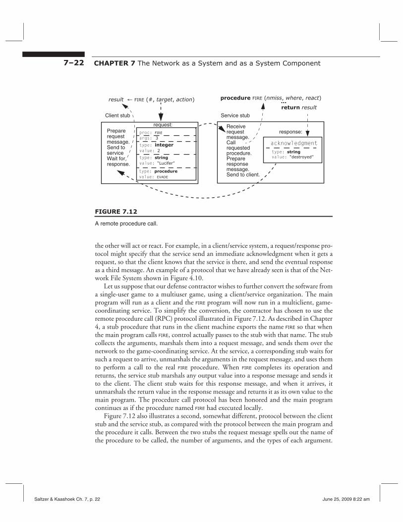
Let us suppose that our defense contractor wishes to further convert the software from a single-user game to a multiuser game, using a client/service organization. The main program will run as a client and the FIRE program will now run in a multiclient, game-coordinating service. To simplify the conversion, the contractor has chosen to use the remote procedure call (RPC) protocol illustrated in Figure 7.12. As described in Chapter 4, a stub procedure that runs in the client machine exports the name FIRE so that when the main program calls FIRE, control actually passes to the stub with that name. The stub collects the arguments, marshals them into a request message, and sends them over the network to the game-coordinating service. At the service, a corresponding stub waits for such a request to arrive, unmarshals the arguments in the request message, and uses them to perform a call to the real FIRE procedure. When FIRE completes its operation and returns, the service stub marshals any output value into a response message and sends it to the client. The client stub waits for this response message, and when it arrives, it unmarshals the return value in the response message and returns it as its own value to the main program. The procedure call protocol has been honored and the main program continues as if the procedure named FIRE had executed locally.
Figure 7.12 also illustrates a second, somewhat different, protocol between the client stub and the service stub, as compared with the protocol between the main program and the procedure it calls. Between the two stubs the request message spells out the name of the procedure to be called, the number of arguments, and the types of each argument.
Saltzer & Kaashoek Ch. 7, p. 22 June 25, 2009 8:22 am

7.2 Getting Organized: Layers 7–23
Main program called procedureapplication protocol
RPC client stub presentation protocol RPC service stub
FIGURE 7.13
Two protocol layers
The details of the protocol between the RPC stubs need have little in common with the corresponding details of the protocol between the original main program and the procedure it calls.
7.2.1 Layers
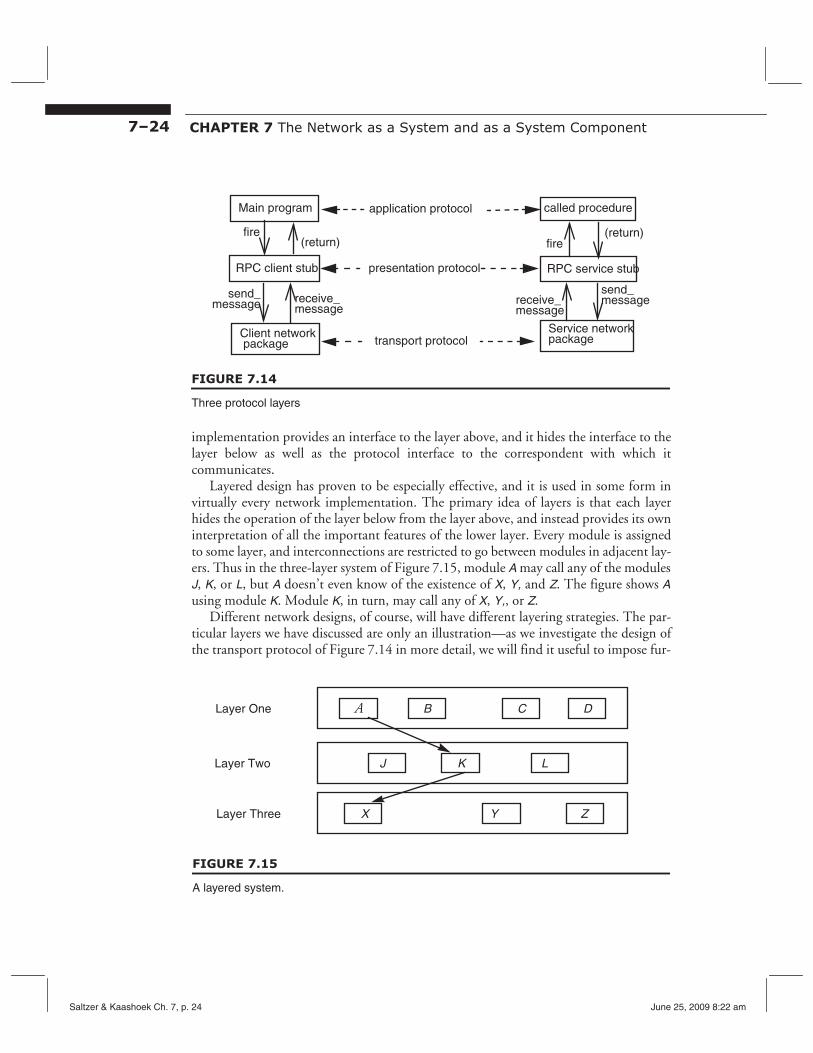
In that example, the independence of the MAIN-to-FIRE procedure call protocol from the RPC stub-to-stub protocol is characteristic of a layered design. We can make those layers explicit by redrawing our picture as in Figure 7.13. The contract between the main program and the procedure it calls is called the application protocol. The contract between the client-side and service-side RPC stubs protocol is known as a presentation protocol because it translates data formats and semantics to and from locally preferred forms.
The request message must get from the client RPC stub to the service RPC stub. To communicate, the client stub calls some network procedure, using an elaboration of the SEND abstraction:
SEND_MESSAGE (request_message, service_name)
specifying in a second argument the identity of the service that should receive this request message. The service stub invokes a similar procedure that provides the RECEIVE abstraction to pick up the message. These two procedures represent a third layer, which provides a transport protocol, and we can extend our layered protocol picture as in Figure 7.14.
This figure makes apparent an important property of layering as used in network designs: every module has not two, but three interfaces. In the usual layered organization, a module has just two interfaces, an interface to the layer above, which hides a second interface to the layer below. But as used in a network, layering involves a third interface. Consider, for example, the RPC client stub in the figure. As expected, it provides an interface that the main program can use, and it uses an interface of the client network package below. But the whole point of the RPC client stub is to construct a request message that convinces its correspondent stub at the service to do something. The presentation protocol thus represents a third interface of the presentation layer module. The presentation module thus hides both the lower layer interface and the presentation protocol from the layer above. This observation is a general one—each layer in a network
Saltzer & Kaashoek Ch. 7, p. 23 June 25, 2009 8:22 am
7–24 CHAPTER 7 The Network as a System and as a System Component
Client network package
fire
send_ receive_
(return)
Main program
RPC client stub
message message
application protocol
presentation protocol
transport protocol Service network package
fire (return)
called procedure
RPC service stub
receive_ message
send_ message
FIGURE 7.14
Three protocol layers
implementation provides an interface to the layer above, and it hides the interface to the layer below as well as the protocol interface to the correspondent with which it communicates.
Layered design has proven to be especially effective, and it is used in some form in virtually every network implementation. The primary idea of layers is that each layer hides the operation of the layer below from the layer above, and instead provides its own interpretation of all the important features of the lower layer. Every module is assigned to some layer, and interconnections are restricted to go between modules in adjacent layers. Thus in the three-layer system of Figure 7.15, module A may call any of the modules J, K, or L, but A doesn’t even know of the existence of X, Y, and Z. The figure shows A using module K. Module K, in turn, may call any of X, Y,, or Z.
Different network designs, of course, will have different layering strategies. The particular layers we have discussed are only an illustration—as we investigate the design of the transport protocol of Figure 7.14 in more detail, we will find it useful to impose fur-
Layer One
Layer Two
Layer Three
A B C D
X Y Z
J K L
FIGURE 7.15
A layered system.
Saltzer & Kaashoek Ch. 7, p. 24 June 25, 2009 8:22 am

7.2 Getting Organized: Layers 7–25
ther layers, using a three-layer reference model that provides quite a bit of insight into how networks are organized. Our choice strongly resembles the layering that is used in the design of the Internet. The three layers we choose divide the problem of implementing a network as follows (from the bottom up):
• The link layer: moving data directly from one point to another. • The network layer: forwarding data through intermediate points to move it to
the place it is wanted. • The end-to-end layer: everything else required to provide a comfortable
application interface.
The application itself can be thought of as a fourth, highest layer, not part of the network. On the other hand, some applications intertwine themselves so thoroughly with the end-to-end layer that it is hard to make a distinction.
The terms frame, packet, segment, message, and stream that were introduced in Section 7.1 can now be identified with these layers. Each is the unit of transmission of one of the protocol layers. Working from the top down, an application starts by asking the end-toend layer to transmit a message or a stream of data to a correspondent. The end-to-end layer splits long messages and streams into segments, it copes with lost or duplicated segments, it places arriving segments in proper order, it enforces specific communication semantics, it performs presentation transformations, and it calls on the network layer to transmit each segment. The network layer accepts segments from the end-to-end layer, constructs packets, and transmits those packets across the network, choosing which links to follow to move a given packet from its origin to its destination. The link layer accepts packets from the network layer, and constructs and transmits frames across a single link between two forwarders or between a forwarder and a customer of the network.
Some network designs attempt to impose a strict layering among various parts of what we call the end-to-end layer, but it is often such a hodgepodge of function that no single layering can describe it in a useful way. On the other hand, the network and link layers are encountered frequently enough in data communication networks that one can almost consider them universal.
With this high-level model in mind, we next sketch the basic contracts for each of the three layers and show how they relate to one another. Later, we examine in much more depth how each of the three layers is actually implemented.
7.2.2 The Link Layer
At the bottom of a packet-switched network there must be some underlying communication mechanism that connects one packet switch with another or a packet switch to a customer of the network. The link layer is responsible for managing this low-level communication. The goal of the link layer is to move the bits of the packet across one (usually, but not necessarily, physical) link, hiding the particular mechanics of data transmission that are involved.
Saltzer & Kaashoek Ch. 7, p. 25 June 25, 2009 8:22 am
7–26 CHAPTER 7 The Network as a System and as a System Component
Link Layer link
protocol link
protocol
link 1 link 2
LINK_SEND (pkt, link2)
Link Layer
Link Layer
A B C
DATA
DATA LH LT
NETWORK_HANDLE
FIGURE 7.16
A link layer in a packet switch that has two physical links
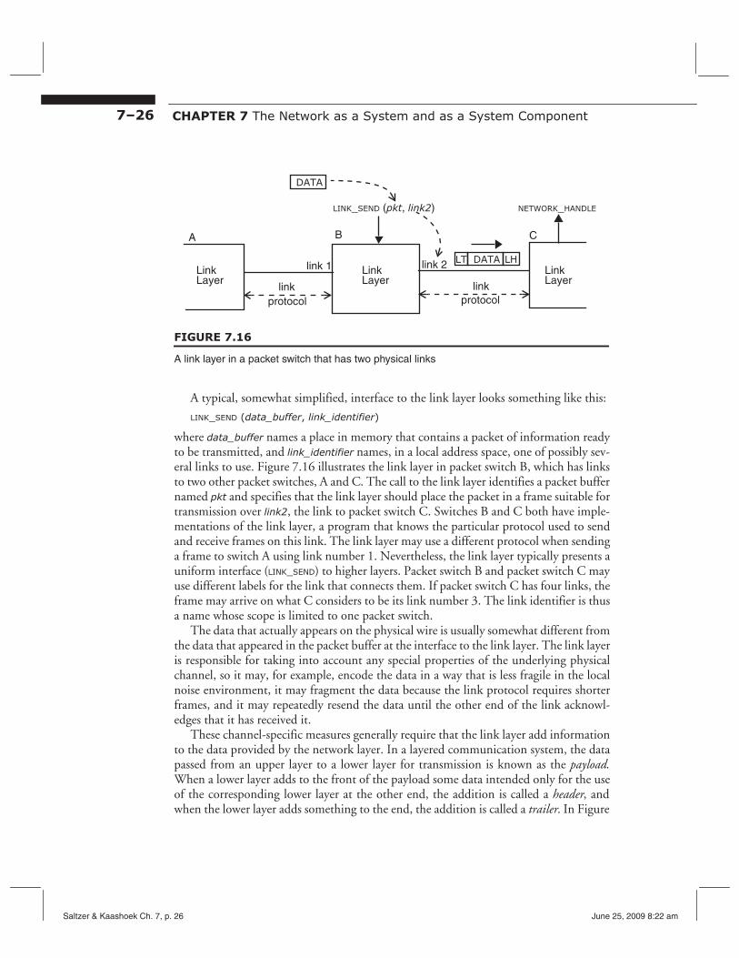
A typical, somewhat simplified, interface to the link layer looks something like this:
LINK_SEND (data_buffer, link_identifier)
where data_buffer names a place in memory that contains a packet of information ready to be transmitted, and link_identifier names, in a local address space, one of possibly several links to use. Figure 7.16 illustrates the link layer in packet switch B, which has links to two other packet switches, A and C. The call to the link layer identifies a packet buffer named pkt and specifies that the link layer should place the packet in a frame suitable for transmission over link2, the link to packet switch C. Switches B and C both have implementations of the link layer, a program that knows the particular protocol used to send and receive frames on this link. The link layer may use a different protocol when sending a frame to switch A using link number 1. Nevertheless, the link layer typically presents a uniform interface (LINK_SEND) to higher layers. Packet switch B and packet switch C may use different labels for the link that connects them. If packet switch C has four links, the frame may arrive on what C considers to be its link number 3. The link identifier is thus a name whose scope is limited to one packet switch.
The data that actually appears on the physical wire is usually somewhat different from the data that appeared in the packet buffer at the interface to the link layer. The link layer is responsible for taking into account any special properties of the underlying physical channel, so it may, for example, encode the data in a way that is less fragile in the local noise environment, it may fragment the data because the link protocol requires shorter frames, and it may repeatedly resend the data until the other end of the link acknowledges that it has received it.
These channel-specific measures generally require that the link layer add information to the data provided by the network layer. In a layered communication system, the data passed from an upper layer to a lower layer for transmission is known as the payload. When a lower layer adds to the front of the payload some data intended only for the use of the corresponding lower layer at the other end, the addition is called a header, and when the lower layer adds something to the end, the addition is called a trailer. In Figure
Saltzer & Kaashoek Ch. 7, p. 26 June 25, 2009 8:22 am
7.2 Getting Organized: Layers 7–27
7.16, the link layer has added a link layer header LH (perhaps indicating which network layer program to deliver the packet to) and a link layer trailer LT (perhaps containing a checksum for error detection). The combination of the header, payload, and trailer becomes the link-layer frame. The receiving link layer module will, after establishing that the frame has been correctly received, remove the link layer header and trailer before passing the payload to the network layer.
The particular method of waiting for a frame, packet, or message to arrive and transferring payload data and control from a lower layer to an upper layer depends on the available thread coordination procedures. Throughout this chapter, rather than having an upper layer call down to a lower-layer procedure named RECEIVE (as Section 2.1.3 suggested), we use upcalls, which means that when data arrives, the lower layer makes a procedure call up to an entry point in the higher layer. Thus in Figure 7.16 the link layer calls a procedure named NETWORK_HANDLE in the layer above.
7.2.3 The Network Layer
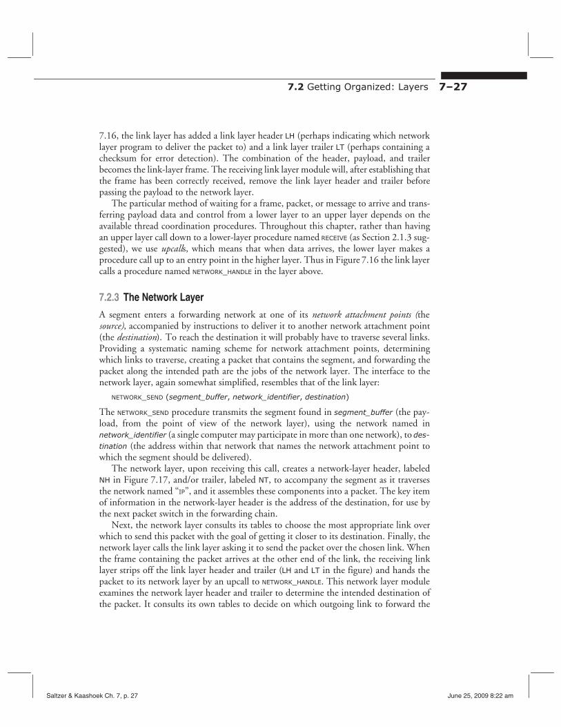
A segment enters a forwarding network at one of its network attachment points (the source), accompanied by instructions to deliver it to another network attachment point (the destination). To reach the destination it will probably have to traverse several links. Providing a systematic naming scheme for network attachment points, determining which links to traverse, creating a packet that contains the segment, and forwarding the packet along the intended path are the jobs of the network layer. The interface to the network layer, again somewhat simplified, resembles that of the link layer:
NETWORK_SEND (segment_buffer, network_identifier, destination)
The NETWORK_SEND procedure transmits the segment found in segment_buffer (the payload, from the point of view of the network layer), using the network named in network_identifier (a single computer may participate in more than one network), to des
tination (the address within that network that names the network attachment point to which the segment should be delivered).
The network layer, upon receiving this call, creates a network-layer header, labeled NH in Figure 7.17, and/or trailer, labeled NT, to accompany the segment as it traverses the network named “IP”, and it assembles these components into a packet. The key item of information in the network-layer header is the address of the destination, for use by the next packet switch in the forwarding chain.
Next, the network layer consults its tables to choose the most appropriate link over which to send this packet with the goal of getting it closer to its destination. Finally, the network layer calls the link layer asking it to send the packet over the chosen link. When the frame containing the packet arrives at the other end of the link, the receiving link layer strips off the link layer header and trailer (LH and LT in the figure) and hands the packet to its network layer by an upcall to NETWORK_HANDLE. This network layer module examines the network layer header and trailer to determine the intended destination of the packet. It consults its own tables to decide on which outgoing link to forward the
Saltzer & Kaashoek Ch. 7, p. 27 June 25, 2009 8:22 am

7–28 CHAPTER 7 The Network as a System and as a System Component
DATA
NETWORK_SEND (segment, “IP”, nap_1197)
Link Layer
link protocol
link 2
lINK_SEND (packet, link2)
Link Layer
Link Layer
Network Layer
network
protocol Network Layer
LINK_SEND (packet, link5)
link5
DATANT NH
DATANT NH LHLT
NETWORK_HANDLE
FIGURE 7.17
Relation between the network layer and the link layer.
packet, and it calls the link layer to send the packet on its way. The network layer of each packet switch along the way repeats this procedure, until the packet traverses the link to its destination. The network layer at the end of that link recognizes that the packet is now at its destination, it extracts the data segment from the packet, and passes that segment to the end-to-end layer, with another upcall.
7.2.4 The End-to-End Layer
We can now put the whole picture together. The network and link layers together provide a best-effort network, which has the “interesting” properties that were listed in Figure 7.11 on page 7–21. These properties may be problematic to an application, and the function of the end-to-end layer is to create a less “interesting” and thus easier to use interface for the application. For example, Figure 7.18 shows the remote procedure call of Figure 7.12 from a different perspective. Here the RPC protocol is viewed as an end-to-end layer of a complete network implementation. As with the lower layers, the end-to-end layer has added a header and a trailer to the data that the application gave it, and inspecting the bits on the wire we now see three distinct headers and trailers, corresponding to the three layers of the network implementation.
The RPC implementation in the end-to-end layer provides several distinct end-toend services, each intended to hide some aspect of the underlying network from its application:
Saltzer & Kaashoek Ch. 7, p. 28 June 25, 2009 8:22 am

7.2 Getting Organized: Layers 7–29
• Presentation services. Translating data formats and emulating the semantics of a procedure call. For this purpose the end-to-end header might contain, for example, a count of the number of arguments in the procedure call.
• Transport services. Dividing streams and messages into segments and dealing with lost, duplicated, and out-of-order segments. For this purpose, the end-to-end header might contain serial numbers of the segments.
• Session services. Negotiating a search, handshake, and binding sequence to locate and prepare to use a service that knows how to perform the requested procedure. For this purpose, the end-to-end header might contain a unique identifier that tells the service which client application is making this call.
Depending on the requirements of the application, different end-to-end layer implementations may provide all, some, or none of these services, and the end-to-end header and trailer may contain various different bits of information.
There is one other important property of this layering that becomes evident in examining Figure 7.18. Each layer considers the payload transmitted by the layer above to be information that it is not expected, or even permitted, to interpret. Thus the end-to-end layer constructs a segment with an end-to-end header and trailer that it hands to the network layer, with the expectation that the network layer will not look inside or perform any actions that require interpretation of the segment. The network layer, in turn, adds a network-layer header and trailer and hands the resulting packet to the link layer, again
FIRE (7, “Lucifer”, evade) FIRE (7, “Lucifer”, evade)
Link Layer
Network Layer
end-to-end
protocol
End-to-End Layer
DATA
DATANT NH LHLT
Link Layer
Link Layer
Link Layer
Network Layer
Network Layer
End-to-End Layer
ET EH
DATAET EH
(RPC) (RPC)
DATANT NHET EH
FIGURE 7.18
Three network layers in action.The arguments of the procedure call become the payload of the end-to-end segment. The network layer forwards the packet across two links on the way from the client to the service.The frame on the wire contains the headers and trailers of three layers.
Saltzer & Kaashoek Ch. 7, p. 29 June 25, 2009 8:22 am
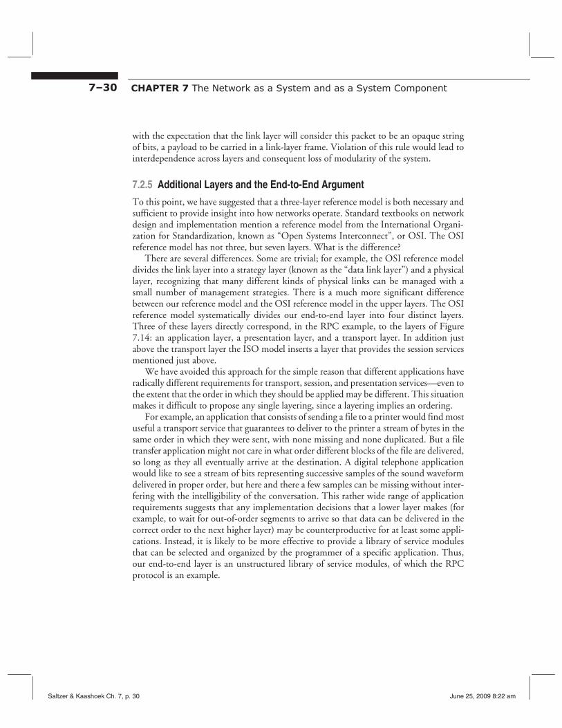
7–30 CHAPTER 7 The Network as a System and as a System Component
with the expectation that the link layer will consider this packet to be an opaque string of bits, a payload to be carried in a link-layer frame. Violation of this rule would lead to interdependence across layers and consequent loss of modularity of the system.
7.2.5 Additional Layers and the End-to-End Argument
To this point, we have suggested that a three-layer reference model is both necessary and sufficient to provide insight into how networks operate. Standard textbooks on network design and implementation mention a reference model from the International Organization for Standardization, known as “Open Systems Interconnect”, or OSI. The OSI reference model has not three, but seven layers. What is the difference?
There are several differences. Some are trivial; for example, the OSI reference model divides the link layer into a strategy layer (known as the “data link layer”) and a physical layer, recognizing that many different kinds of physical links can be managed with a small number of management strategies. There is a much more significant difference between our reference model and the OSI reference model in the upper layers. The OSI reference model systematically divides our end-to-end layer into four distinct layers. Three of these layers directly correspond, in the RPC example, to the layers of Figure 7.14: an application layer, a presentation layer, and a transport layer. In addition just above the transport layer the ISO model inserts a layer that provides the session services mentioned just above.
We have avoided this approach for the simple reason that different applications have radically different requirements for transport, session, and presentation services—even to the extent that the order in which they should be applied may be different. This situation makes it difficult to propose any single layering, since a layering implies an ordering.
For example, an application that consists of sending a file to a printer would find most useful a transport service that guarantees to deliver to the printer a stream of bytes in the same order in which they were sent, with none missing and none duplicated. But a file transfer application might not care in what order different blocks of the file are delivered, so long as they all eventually arrive at the destination. A digital telephone application would like to see a stream of bits representing successive samples of the sound waveform delivered in proper order, but here and there a few samples can be missing without interfering with the intelligibility of the conversation. This rather wide range of application requirements suggests that any implementation decisions that a lower layer makes (for example, to wait for out-of-order segments to arrive so that data can be delivered in the correct order to the next higher layer) may be counterproductive for at least some applications. Instead, it is likely to be more effective to provide a library of service modules that can be selected and organized by the programmer of a specific application. Thus, our end-to-end layer is an unstructured library of service modules, of which the RPC protocol is an example.
Saltzer & Kaashoek Ch. 7, p. 30 June 25, 2009 8:22 am

7.2 Getting Organized: Layers 7–31
This argument against additional layers is an example of a design principle known as
The end-to-end argument
The application knows best.
In this case, the basic thrust of the end-to-end argument is that the application knows best what its real communication requirements are, and for a lower network layer to try to implement any feature other than transporting the data risks implementing something that isn’t quite what the application needed. Moreover, if it isn’t exactly what is needed, the application will probably have to reimplement that function on its own. The end-toend argument can thus be paraphrased as: don’t bury it in a lower layer, let the end points deal with it because they know best what they need.
A simple example of this phenomenon is file transfer. To transfer a file carefully, the appropriate method is to calculate a checksum from the contents of the file as it is stored in the file system of the originating site. Then, after the file has been transferred and written to the new file system, the receiving site should read the file back out of its file system, recalculate the checksum anew, and compare it with the original checksum. If the two checksums are the same, the file transfer application has quite a bit of confidence that the new site has a correct copy; if they are different, something went wrong and recovery is needed.
Given this end-to-end approach to checking the accuracy of the file transfer, one can question whether or not there is any value in, for example, having the link layer protocol add a frame checksum to the link layer trailer. This link layer checksum takes time to calculate, it adds to the data to be sent, and it verifies the correctness of the data only while it is being transmitted across that link. Despite this protection, the data may still be damaged while it is being passed through the network layer, or while it is buffered by the receiving part of the file transfer application, or while it is being written to the disk. Because of those threats, the careful file transfer application cannot avoid calculating its end-to-end checksum, despite the protection provided by the link layer checksum.
This is not to say that the link layer checksum is worthless. If the link layer provides a checksum, that layer will discover data transmission errors at a time when they can be easily corrected by resending just one frame. Absent this link-layer checksum, a transmission error will not be discovered until the end-to-end layer verifies its checksum, by which point it may be necessary to redo the entire file transfer. So there may be a significant performance gain in having this feature in a lower-level layer. The interesting observation is that a lower-layer checksum does not eliminate the need for the application layer to implement the function, and it is thus not required for application correctness. It is just a performance enhancement.
The end-to-end argument can be applied to a variety of system design issues in addition to network design. It does not provide an absolute decision technique, but rather a useful argument that should be weighed against other arguments in deciding where to place function.
Saltzer & Kaashoek Ch. 7, p. 31 June 25, 2009 8:22 am
7–32 CHAPTER 7 The Network as a System and as a System Component
7.2.6 Mapped and Recursive Applications of the Layered Model
When one begins decomposing a particular existing network into link, network, and end-to-end layers, it sometimes becomes apparent that some of the layers of the network are themselves composed of what are obviously link, network, or end-to-end layers. These compositions come in two forms: mapped and recursive.
Mapped composition occurs when a network layer is built directly on another network layer by mapping higher-layer network addresses to lower-layer network addresses. A typical application for mapping arises when a better or more popular network technology comes along, yet it is desirable to keep running applications that are designed for the old network. For example, Apple designed a network called Appletalk that was used for many years, and then later mapped the Appletalk network layer to the Ethernet, which, as described in Section 7.8, has a network and link layer of its own but uses a somewhat different scheme for its network layer addresses.
Another application for mapped composition is to interconnect several independently designed network layers, a scheme called internetworking. Probably the best example of internetworking is the Internet itself (described in Sidebar 7.2), which links together many different network layers by mapping them all to a universal network layer that uses a protocol known as Internet protocol (IP). Section 7.8 explains how the network
Sidebar 7.2: The Internet The Internet provides examples of nearly every concept in this chapter. Much of the Internet is a network layer that is mapped onto some other network layer such as a satellite network, a wireless network, or an Ethernet. Internet protocol (IP) is the primary network layer protocol, but it is not the only network layer protocol used in the Internet. There is a network layer protocol for managing the Internet, known as ICMP. There are also several different network layer routing protocols, some providing routing within small parts of the Internet, others providing routing between major regions. But every point that can be reached via the Internet implements IP.
The link layer of the Internet includes all of the link layers of the networks that the Internet maps onto and it also includes many separate, specialized links: a wire, a dial-up telephone line, a dedicated line provided by the telephone company, a microwave link, a digital subscriber line (DSL), a free-space optical link, etc. Almost anything that carries bits has been used somewhere as a link in the Internet.
The end-to-end protocols used on the Internet are many and varied. The primary transport protocols are TCP, UDP, and RTP, described briefly on page 7–65. Built on these transport protocols are hundreds of application protocols. A short list of some of the most widely used application protocols would include file transfer (FTP), the World Wide Web (HTTP), mail dispatch and pickup (SMTP and POP), text messaging (IRC), telephone (VoIP), and file exchange (Gnutella, bittorrent, etc.).
The current chapter presents a general model of networks, rather than a description of the Internet. To learn more about the Internet, see the books and papers listed in Section 7 of the Suggestions for Further Reading.
Saltzer & Kaashoek Ch. 7, p. 32 June 25, 2009 8:22 am
7.2 Getting Organized: Layers 7–33
layer addresses of the Ethernet are mapped to and from the IP addresses of the Internet using what is known as an Address Resolution Protocol. The Internet also maps the internal network addresses of many other networks—wireless networks, satellite networks, cable TV networks, etc.—into IP addresses.
Recursive composition occurs when a network layer rests on a link layer that itself is a complete three-layer network. Recursive composition is not a general property of layers, but rather it is a specific property of layered communication systems: The send/receive semantics of an end-to-end connection through a network can be designed to be have the same semantics as a single link, so such an end-to-end connection can be used as a link in a higher-level network. That property facilitates recursive composition, as well as the implementation of various interesting and useful network structures. Here are some examples of recursive composition:
• A dial-up telephone line is often used as a link to an attachment point of the Internet. This dial-up line goes through a telephone network that has its own link, network, and end-to-end layers.
• An overlay network is a network layer structure that uses as links the end-to-end layer of an existing network. Gnutella (see problem set 20) is an example of an overlay network that uses the end-to-end layer of the Internet for its links.
• With the advance of “voice over IP” (VoIP), the traditional voice telephone network is gradually converting to become an overlay on the Internet.
• A tunnel is a structure that uses the end-to-end layer of an existing network as a link between a local network-layer attachment point and a distant one to make it appear that the attachment is at the distant point. Tunnels, combined with the encryption techniques described in Chapter 11, are used to implement what is commonly called a “virtual private network” (VPN).
Recursive composition need not be limited to two levels. Figure 7.19 illustrates the case of Gnutella overlaying the Internet, with a dial-up telephone connection being used as the Internet link layer.
The primary concern when one is dealing with a link layer that is actually an end-toend connection through another network is that discussion can become confusing unless one is careful to identify which level of decomposition is under discussion. Fortunately our terminology helps keep track of the distinctions among the various layers of a network, so it is worth briefly reviewing that terminology. At the interface between the application and the end-to-end layer, data is identified as a stream or message. The end-to-end layer divides the stream or message up into a series of segments and hands them to the network layer for delivery. The network layer encapsulates each segment in a packet which it forwards through the network with the help of the link layer. The link layer transmits the packet in a frame. If the link layer is itself a network, then this frame is a message as viewed by the underlying network.
This discussion of layered network organization has been both general and abstract. In the next three sections we investigate in more depth the usual functions and some typ-
Saltzer & Kaashoek Ch. 7, p. 33 June 25, 2009 8:22 am

7–34 CHAPTER 7 The Network as a System and as a System Component
File Transfer Program (end-to-end layer) File transfer system
Gnutella (network layer)
Transport Protocol (end-to-end layer) Internet
Internet Protocol (network layer) (linklayer)
dialed connection (end-to-end layer) dial-uptelephone
telephone switch (network layer) (link networklayer)physical wire (link layer)
FIGURE 7.19
A typical recursive network composition.The overlay network Gnutella uses for its link layer an end-to-end transport protocol of the Internet. The Internet uses for one of its links an end-toend transport protocol of the dial-up telephone system.
ical implementation techniques of each of the three layers of our reference model. However, as the introduction pointed out, what follows is not a comprehensive treatment of networking. Instead it identifies many of the major issues and for each issue exhibits one or two examples of how that issue is typically handled in a real network design. For readers who have a goal of becoming network engineers, and who therefore would like to learn the whole remarkable range of implementation strategies that have been used in networks, the Suggestions for Further Reading list several comprehensive books on the subject.
7.3 The Link Layer The link layer is the bottom-most of the three layers of our reference model. The link layer is responsible for moving data directly from one physical location to another. It thus gets involved in several distinct issues: physical transmission, framing bits and bit sequences, detecting transmission errors, multiplexing the link, and providing a useful interface to the network layer above.
7.3.1 Transmitting Digital Data in an Analog World
The purpose of the link layer is to move bits from one place to another. If we are talking about moving a bit from one register to another on the same chip, the mechanism is fairly simple: run a wire that connects the output of the first register to the input of the next. Wait until the first register’s output has settled and the signal has propagated to the input of the second; the next clock tick reads the data into the second register. If all of the volt-
Saltzer & Kaashoek Ch. 7, p. 34 June 25, 2009 8:22 am
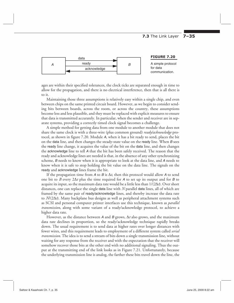
7.3 The Link Layer 7–35
A
FIGURE 7.20data
ready B A simple protocol for data acknowledge communication.
ages are within their specified tolerances, the clock ticks are separated enough in time to allow for the propagation, and there is no electrical interference, then that is all there is to it.
Maintaining those three assumptions is relatively easy within a single chip, and even between chips on the same printed circuit board. However, as we begin to consider sending bits between boards, across the room, or across the country, these assumptions become less and less plausible, and they must be replaced with explicit measures to ensure that data is transmitted accurately. In particular, when the sender and receiver are in separate systems, providing a correctly timed clock signal becomes a challenge.
A simple method for getting data from one module to another module that does not share the same clock is with a three-wire (plus common ground) ready/acknowledge protocol, as shown in figure 7.20. Module A, when it has a bit ready to send, places the bit on the data line, and then changes the steady-state value on the ready line. When B sees the ready line change, it acquires the value of the bit on the data line, and then changes the acknowledge line to tell A that the bit has been safely received. The reason that the ready and acknowledge lines are needed is that, in the absence of any other synchronizing scheme, B needs to know when it is appropriate to look at the data line, and A needs to know when it is safe to stop holding the bit value on the data line. The signals on the ready and acknowledge lines frame the bit.
If the propagation time from A to B is Δt, then this protocol would allow A to send one bit to B every 2Δt plus the time required for A to set up its output and for B to acquire its input, so the maximum data rate would be a little less than 1/(2Δt). Over short distances, one can replace the single data line with N parallel data lines, all of which are framed by the same pair of ready/acknowledge lines, and thereby increase the data rate to N/(2Δt). Many backplane bus designs as well as peripheral attachment systems such as SCSI and personal computer printer interfaces use this technique, known as parallel transmission, along with some variant of a ready/acknowledge protocol, to achieve a higher data rate.
However, as the distance between A and B grows, Δt also grows, and the maximum data rate declines in proportion, so the ready/acknowledge technique rapidly breaks down. The usual requirement is to send data at higher rates over longer distances with fewer wires, and this requirement leads to employment of a different system called serial transmission. The idea is to send a stream of bits down a single transmission line, without waiting for any response from the receiver and with the expectation that the receiver will somehow recover those bits at the other end with no additional signaling. Thus the output at the transmitting end of the link looks as in Figure 7.21. Unfortunately, because the underlying transmission line is analog, the farther these bits travel down the line, the
Saltzer & Kaashoek Ch. 7, p. 35 June 25, 2009 8:22 am
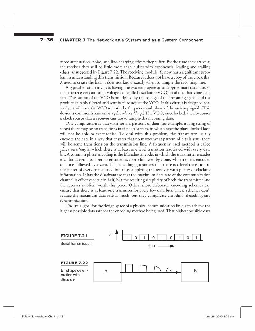
7–36 CHAPTER 7 The Network as a System and as a System Component
more attenuation, noise, and line-charging effects they suffer. By the time they arrive at the receiver they will be little more than pulses with exponential leading and trailing edges, as suggested by Figure 7.22. The receiving module, B, now has a significant problem in understanding this transmission: Because it does not have a copy of the clock that A used to create the bits, it does not know exactly when to sample the incoming line.
A typical solution involves having the two ends agree on an approximate data rate, so that the receiver can run a voltage-controlled oscillator (VCO) at about that same data rate. The output of the VCO is multiplied by the voltage of the incoming signal and the product suitably filtered and sent back to adjust the VCO. If this circuit is designed correctly, it will lock the VCO to both the frequency and phase of the arriving signal. (This device is commonly known as a phase-locked loop.) The VCO, once locked, then becomes a clock source that a receiver can use to sample the incoming data.
One complication is that with certain patterns of data (for example, a long string of zeros) there may be no transitions in the data stream, in which case the phase-locked loop will not be able to synchronize. To deal with this problem, the transmitter usually encodes the data in a way that ensures that no matter what pattern of bits is sent, there will be some transitions on the transmission line. A frequently used method is called phase encoding, in which there is at least one level transition associated with every data bit. A common phase encoding is the Manchester code, in which the transmitter encodes each bit as two bits: a zero is encoded as a zero followed by a one, while a one is encoded as a one followed by a zero. This encoding guarantees that there is a level transition in the center of every transmitted bit, thus supplying the receiver with plenty of clocking information. It has the disadvantage that the maximum data rate of the communication channel is effectively cut in half, but the resulting simplicity of both the transmitter and the receiver is often worth this price. Other, more elaborate, encoding schemes can ensure that there is at least one transition for every few data bits. These schemes don’t reduce the maximum data rate as much, but they complicate encoding, decoding, and synchronization.
The usual goal for the design space of a physical communication link is to achieve the highest possible data rate for the encoding method being used. That highest possible data
FIGURE 7.21 V
Serial transmission. time
1 1 1 1 10 0 0 0
A B
FIGURE 7.22
Bit shape deterioration with distance.
Saltzer & Kaashoek Ch. 7, p. 36 June 25, 2009 8:22 am
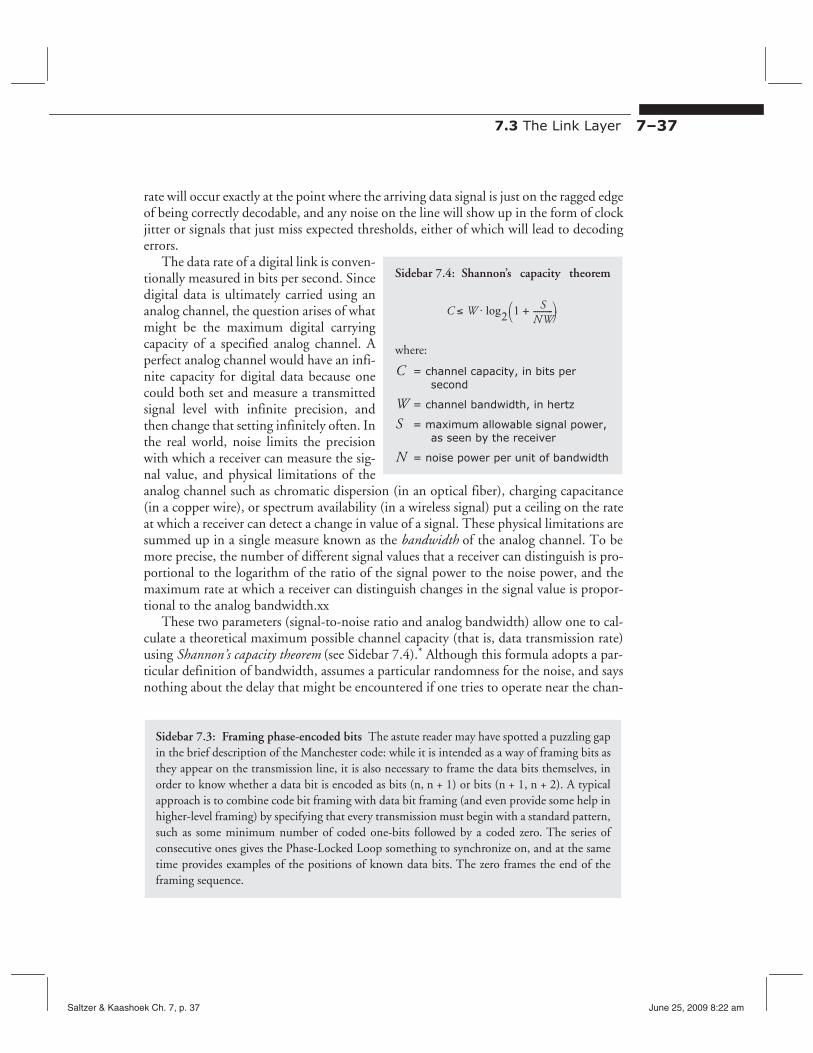
7.3 The Link Layer 7–37
rate will occur exactly at the point where the arriving data signal is just on the ragged edge of being correctly decodable, and any noise on the line will show up in the form of clock jitter or signals that just miss expected thresholds, either of which will lead to decoding errors.
The data rate of a digital link is conventionally measured in bits per second. Since Sidebar 7.4: Shannon’s capacity theorem
digital data is ultimately carried using an ≤ ⎛1 + S ⎞analog channel, the question arises of what C W ⋅ log ---------2⎝ NW⎠
might be the maximum digital carrying capacity of a specified analog channel. A where: perfect analog channel would have an infinite capacity for digital data because one C = channel capacity, in bits per
secondcould both set and measure a transmitted signal level with infinite precision, and W = channel bandwidth, in hertz
then change that setting infinitely often. In S = maximum allowable signal power,
the real world, noise limits the precision as seen by the receiver
with which a receiver can measure the sig- N = noise power per unit of bandwidth
nal value, and physical limitations of the analog channel such as chromatic dispersion (in an optical fiber), charging capacitance (in a copper wire), or spectrum availability (in a wireless signal) put a ceiling on the rate at which a receiver can detect a change in value of a signal. These physical limitations are summed up in a single measure known as the bandwidth of the analog channel. To be more precise, the number of different signal values that a receiver can distinguish is proportional to the logarithm of the ratio of the signal power to the noise power, and the maximum rate at which a receiver can distinguish changes in the signal value is proportional to the analog bandwidth.xx
These two parameters (signal-to-noise ratio and analog bandwidth) allow one to calculate a theoretical maximum possible channel capacity (that is, data transmission rate) using Shannon’s capacity theorem (see Sidebar 7.4).* Although this formula adopts a particular definition of bandwidth, assumes a particular randomness for the noise, and says nothing about the delay that might be encountered if one tries to operate near the chan-
Sidebar 7.3: Framing phase-encoded bits The astute reader may have spotted a puzzling gap in the brief description of the Manchester code: while it is intended as a way of framing bits as they appear on the transmission line, it is also necessary to frame the data bits themselves, in order to know whether a data bit is encoded as bits (n, n + 1) or bits (n + 1, n + 2). A typical approach is to combine code bit framing with data bit framing (and even provide some help in higher-level framing) by specifying that every transmission must begin with a standard pattern, such as some minimum number of coded one-bits followed by a coded zero. The series of consecutive ones gives the Phase-Locked Loop something to synchronize on, and at the same time provides examples of the positions of known data bits. The zero frames the end of the framing sequence.
Saltzer & Kaashoek Ch. 7, p. 37 June 25, 2009 8:22 am
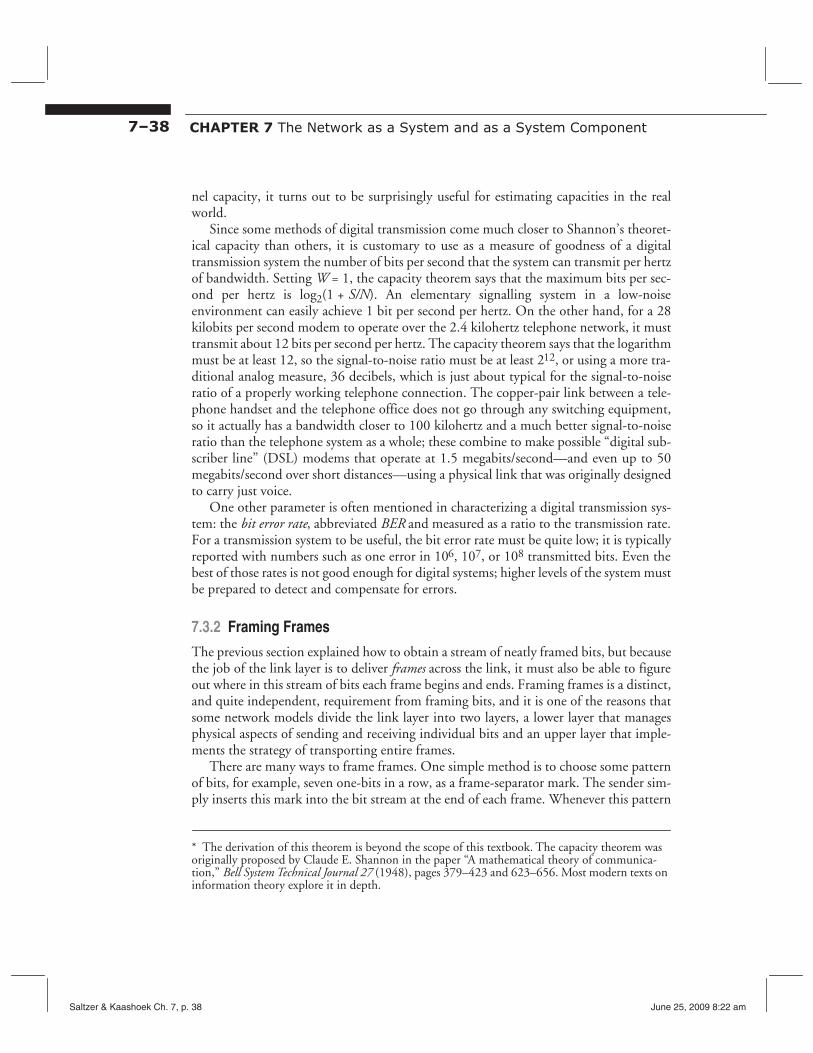
7–38 CHAPTER 7 The Network as a System and as a System Component
nel capacity, it turns out to be surprisingly useful for estimating capacities in the real world.
Since some methods of digital transmission come much closer to Shannon’s theoretical capacity than others, it is customary to use as a measure of goodness of a digital transmission system the number of bits per second that the system can transmit per hertz of bandwidth. Setting W = 1, the capacity theorem says that the maximum bits per second per hertz is log2(1 + S/N). An elementary signalling system in a low-noise environment can easily achieve 1 bit per second per hertz. On the other hand, for a 28 kilobits per second modem to operate over the 2.4 kilohertz telephone network, it must transmit about 12 bits per second per hertz. The capacity theorem says that the logarithm must be at least 12, so the signal-to-noise ratio must be at least 212, or using a more traditional analog measure, 36 decibels, which is just about typical for the signal-to-noise ratio of a properly working telephone connection. The copper-pair link between a telephone handset and the telephone office does not go through any switching equipment, so it actually has a bandwidth closer to 100 kilohertz and a much better signal-to-noise ratio than the telephone system as a whole; these combine to make possible “digital subscriber line” (DSL) modems that operate at 1.5 megabits/second—and even up to 50 megabits/second over short distances—using a physical link that was originally designed to carry just voice.
One other parameter is often mentioned in characterizing a digital transmission system: the bit error rate, abbreviated BER and measured as a ratio to the transmission rate. For a transmission system to be useful, the bit error rate must be quite low; it is typically reported with numbers such as one error in 106, 107, or 108 transmitted bits. Even the best of those rates is not good enough for digital systems; higher levels of the system must be prepared to detect and compensate for errors.
7.3.2 Framing Frames
The previous section explained how to obtain a stream of neatly framed bits, but because the job of the link layer is to deliver frames across the link, it must also be able to figure out where in this stream of bits each frame begins and ends. Framing frames is a distinct, and quite independent, requirement from framing bits, and it is one of the reasons that some network models divide the link layer into two layers, a lower layer that manages physical aspects of sending and receiving individual bits and an upper layer that implements the strategy of transporting entire frames.
There are many ways to frame frames. One simple method is to choose some pattern of bits, for example, seven one-bits in a row, as a frame-separator mark. The sender simply inserts this mark into the bit stream at the end of each frame. Whenever this pattern
* The derivation of this theorem is beyond the scope of this textbook. The capacity theorem was originally proposed by Claude E. Shannon in the paper “A mathematical theory of communication,” Bell System Technical Journal 27 (1948), pages 379–423 and 623–656. Most modern texts on information theory explore it in depth.
Saltzer & Kaashoek Ch. 7, p. 38 June 25, 2009 8:22 am

7.3 The Link Layer 7–39
appears in the received data, the receiver takes it to mark the end of the previous frame, and assumes that any bits that follow belong to the next frame. This scheme works nicely, as long as the payload data stream never contains the chosen pattern of bits.
Rather than explaining to the higher layers of the network that they cannot transmit certain bit patterns, the link layer implements a technique known as bit stuffing. The transmitting end of the link layer, in addition to inserting the frame-separator mark between frames, examines the data stream itself, and if it discovers six ones in a row it stuffs an extra bit into the stream, a zero. The receiver, in turn, watches the incoming bit stream for long strings of ones. When it sees six one-bits in a row it examines the next bit to decide what to do. If the seventh bit is a zero, the receiver discards the zero bit, thus reversing the stuffing done by the sender. If the seventh bit is a one, the receiver takes the seven ones as the frame separator. Figure shows a simple pseudocode implementation of the procedure to send a frame with bit stuffing, and Figure 7.24 shows the corresponding procedure on the receiving side of the link. (For simplicity, the illustrated receive procedure ignores two important considerations. First, the receiver uses only one frame buffer. A better implementation would have multiple buffers to allow it to receive the next frame while processing the current one. Second, the same thread that acquires a bit also runs the network level protocol by calling LINK_RECEIVE. A better implementation would probably NOTIFY a separate thread that would then call the higher-level protocol, and this thread could continue processing more incoming bits.)
Bit stuffing is one of many ways to frame frames. There is little need to explore all the possible alternatives because frame framing is easily specified and subcontracted to the implementer of the link layer—the entire link layer, along with bit framing, is often done in the hardware—so we now move on to other issues.
procedure FRAME_TO_BIT (frame_data, length) ones_in_a_row = 0 for i from 1 to length do // First send frame contents
SEND_BIT (frame_data[i]); if frame_data[i] = 1 then
ones_in_a_row ← ones_in_a_row + 1; if ones_in_a_row = 6 then
SEND_BIT (0); // Stuff a zero so that data doesn’t ones_in_a_row ← 0; // look like a framing marker
else ones_in_a_row ← 0;
for i from 1 to 7 do // Now send framing marker. SEND_BIT (1)
FIGURE 7.23
Sending a frame with bit stuffing.
Saltzer & Kaashoek Ch. 7, p. 39 June 25, 2009 8:22 am

7–40 CHAPTER 7 The Network as a System and as a System Component
7.3.3 Error Handling
An important issue is what the receiving side of the link layer should do about bits that arrive with doubtful values. Since the usual design pushes the data rate of a transmission link up until the receiver can barely tell the ones from the zeros, even a small amount of extra noise can cause errors in the received bit stream.
The first and perhaps most important line of defense in dealing with transmission errors is to require that the design of the link be good at detecting such errors when they occur. The usual method is to encode the data with an error detection code, which entails adding a small amount of redundancy. A simple form of such a code is to have the transmitter calculate a checksum and place the checksum at the end of each frame. As soon as the receiver has acquired a complete frame, it recalculates the checksum and compares its result with the copy that came with the frame. By carefully designing the checksum algorithm and making the number of bits in the checksum large enough, one can make the probability of not detecting an error as low as desired. The more interesting issue is what to do when an error is detected. There are three alternatives:
1. Have the sender encode the transmission using an error correction code, which is a code that has enough redundancy to allow the receiver to identify the particular bits that have errors and correct them. This technique is widely used in situations where the noise behavior of the transmission channel is well understood and the redundancy can be targeted to correct the most likely errors. For example, compact disks are recorded with a burst error-correction code designed to cope particularly well with dust and scratches. Error correction is one of the topics of Chapter 8[online].
procedure BIT_TO_FRAME (rcvd_bit) ones_in_a_row integer initially 0 if ones_in_a_row < 6 then
bits_in_frame ← bits_in_frame + 1 frame_data[bits_in_frame] ← rcvd_bit if rcvd_bit = 1 then ones_in_a_row ← ones_in_a_row + 1 else ones_in_a_row ← 0
else // This may be a seventh one-bit in a row, check it out. if rcvd_bit = 0 then
ones_in_a_row ← 0 // Stuffed bit, don't use it. else // This is the end-of-frame marker
LINK_RECEIVE (frame_data, (bits_in_frame - 6), link_id) bits_in_frame ← 0 ones_in_a_row ← 0
FIGURE 7.24
Receiving a frame with bit stuffing.
Saltzer & Kaashoek Ch. 7, p. 40 June 25, 2009 8:22 am

7.3 The Link Layer 7–41
2. Ask the sender to retransmit the frame that contained an error. This alternative requires that the sender hold the frame in a buffer until the receiver has had a chance to recalculate and compare its checksum. The sender needs to know when it is safe to reuse this buffer for another frame. In most such designs the receiver explicitly acknowledges the correct (or incorrect) receipt of every frame. If the propagation time from sender to receiver is long compared with the time required to send a single frame, there may be several frames in flight, and acknowledgments (especially the ones that ask for retransmission) are disruptive. On a high-performance link an explicit acknowledgment system can be surprisingly complex.
3. Let the receiver discard the frame. This alternative is a reasonable choice in light of our previous observation (see page 7–12) that congestion in higher network levels must be handled by discarding packets anyway. Whatever higher-level protocol is used to deal with those discarded packets will also take care of any frames that are discarded because they contained errors.
Real-world designs often involve blending these techniques, for example by having the sender apply a simple error-correction code that catches and repairs the most common errors and that reliably detects and reports any more complex irreparable errors, and then by having the receiver discard the frames that the error-correction code could not repair.
7.3.4 The Link Layer Interface: Link Protocols and Multiplexing
The link layer, in addition to sending bits and frames at one end and receiving them at the other end, also has interfaces to the network layer above, as illustrated in Figure 7.16 on page 7–26. As described so far, the interface consists of an ordinary procedure call (to LINK_SEND) that the network layer uses to tell the link layer to send a packet, and an upcall (to NETWORK_HANDLE) from the link layer to the network layer at the other end to alert the network layer that a packet arrived.
To be practical, this interface between the network layer and the link layer needs to be expanded slightly to incorporate two additional features not previously mentioned: multiple lower-layer protocols, and higher-layer protocol multiplexing. To support these two functions we add two arguments to LINK_SEND, named link_protocol and network_protocol:
LINK_SEND (data_buffer, link_identifier, link_protocol, network_protocol)
Over any given link, it is sometimes appropriate to use different protocols at different times. For example, a wireless link may occasionally encounter a high noise level and need to switch from the usual link protocol to a “robustness” link protocol that employs a more expensive form of error detection with repeated retry, but runs more slowly. At other times it may want to try out a new, experimental link protocol. The third argument to LINK_SEND, link_protocol tells LINK_SEND which link protocol to use for this_data, and its addition leads to the protocol layering illustrated in Figure 7.25.
Saltzer & Kaashoek Ch. 7, p. 41 June 25, 2009 8:22 am
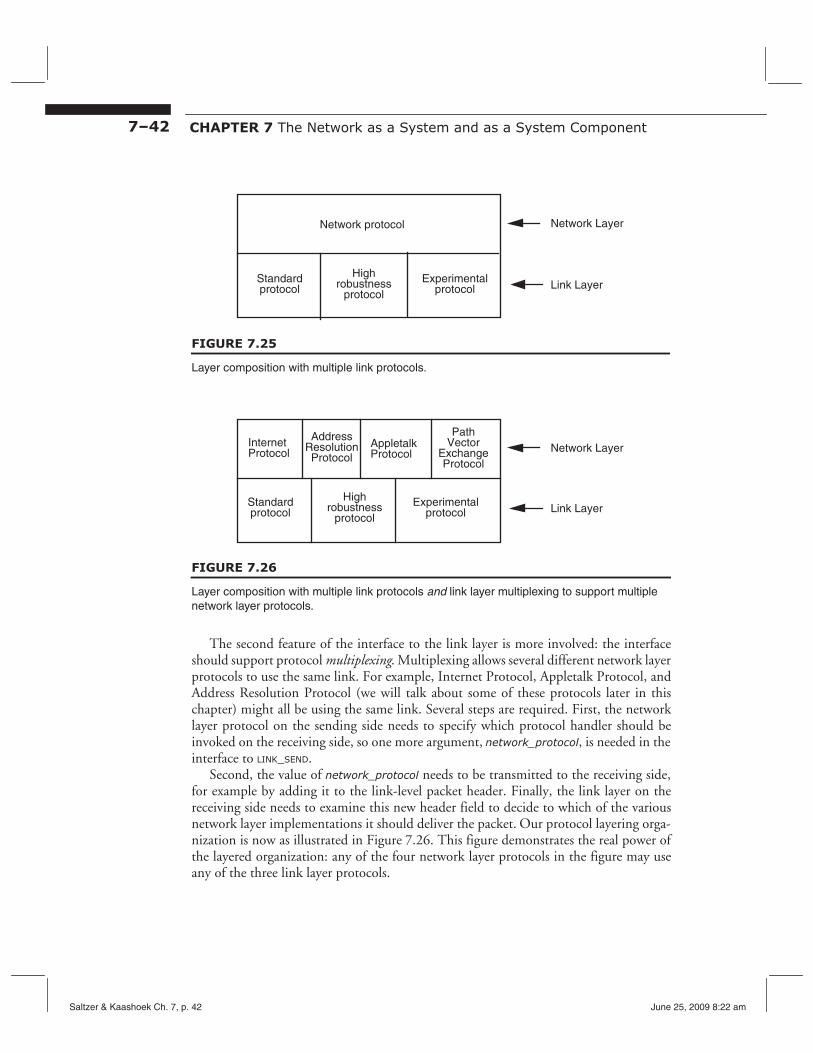
7–42 CHAPTER 7 The Network as a System and as a System Component
Network protocol
Standard High robustness
protocolprotocol
Network Layer
Link LayerExperimental protocol
FIGURE 7.25
Layer composition with multiple link protocols.
Internet Protocol
Address Resolution Protocol
Appletalk Protocol
Path Vector
Exchange Protocol
Standard protocol
High robustness
protocol Experimental
protocol
Network Layer
Link Layer
FIGURE 7.26
Layer composition with multiple link protocols and link layer multiplexing to support multiple network layer protocols.
The second feature of the interface to the link layer is more involved: the interface should support protocol multiplexing. Multiplexing allows several different network layer protocols to use the same link. For example, Internet Protocol, Appletalk Protocol, and Address Resolution Protocol (we will talk about some of these protocols later in this chapter) might all be using the same link. Several steps are required. First, the network layer protocol on the sending side needs to specify which protocol handler should be invoked on the receiving side, so one more argument, network_protocol, is needed in the interface to LINK_SEND.
Second, the value of network_protocol needs to be transmitted to the receiving side, for example by adding it to the link-level packet header. Finally, the link layer on the receiving side needs to examine this new header field to decide to which of the various network layer implementations it should deliver the packet. Our protocol layering organization is now as illustrated in Figure 7.26. This figure demonstrates the real power of the layered organization: any of the four network layer protocols in the figure may use any of the three link layer protocols.
Saltzer & Kaashoek Ch. 7, p. 42 June 25, 2009 8:22 am
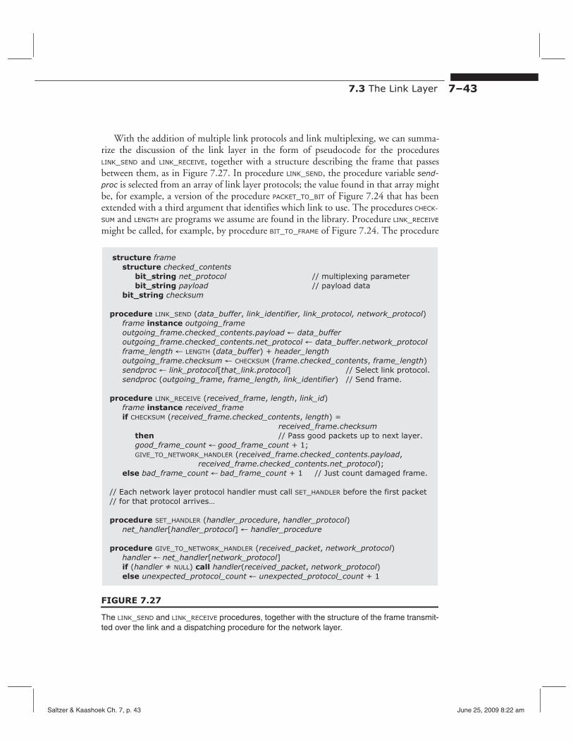
7.3 The Link Layer 7–43
With the addition of multiple link protocols and link multiplexing, we can summarize the discussion of the link layer in the form of pseudocode for the procedures LINK_SEND and LINK_RECEIVE, together with a structure describing the frame that passes between them, as in Figure 7.27. In procedure LINK_SEND, the procedure variable send
proc is selected from an array of link layer protocols; the value found in that array might be, for example, a version of the procedure PACKET_TO_BIT of Figure 7.24 that has been extended with a third argument that identifies which link to use. The procedures CHECK
SUM and LENGTH are programs we assume are found in the library. Procedure LINK_RECEIVE
might be called, for example, by procedure BIT_TO_FRAME of Figure 7.24. The procedure
structure frame structure checked_contents
bit_string net_protocol // multiplexing parameter bit_string payload // payload data
bit_string checksum
procedure LINK_SEND (data_buffer, link_identifier, link_protocol, network_protocol) frame instance outgoing_frame outgoing_frame.checked_contents.payload ← data_buffer outgoing_frame.checked_contents.net_protocol ← data_buffer.network_protocol frame_length ← LENGTH (data_buffer) + header_length outgoing_frame.checksum ← CHECKSUM (frame.checked_contents, frame_length) sendproc ← link_protocol[that_link.protocol] // Select link protocol. sendproc (outgoing_frame, frame_length, link_identifier) // Send frame.
procedure LINK_RECEIVE (received_frame, length, link_id) frame instance received_frame if CHECKSUM (received_frame.checked_contents, length) =
received_frame.checksum then // Pass good packets up to next layer. good_frame_count ← good_frame_count + 1; GIVE_TO_NETWORK_HANDLER (received_frame.checked_contents.payload,
received_frame.checked_contents.net_protocol); else bad_frame_count ← bad_frame_count + 1 // Just count damaged frame.
// Each network layer protocol handler must call SET_HANDLER before the first packet // for that protocol arrives…
procedure SET_HANDLER (handler_procedure, handler_protocol) net_handler[handler_protocol] ← handler_procedure
procedure GIVE_TO_NETWORK_HANDLER (received_packet, network_protocol) handler ← net_handler[network_protocol] if (handler ≠ NULL) call handler(received_packet, network_protocol) else unexpected_protocol_count ← unexpected_protocol_count + 1
FIGURE 7.27
The LINK_SEND and LINK_RECEIVE procedures, together with the structure of the frame transmitted over the link and a dispatching procedure for the network layer.
Saltzer & Kaashoek Ch. 7, p. 43 June 25, 2009 8:22 am

7–44 CHAPTER 7 The Network as a System and as a System Component
LINK_RECEIVE verifies the checksum, and then extracts net_data and net_protocol from the frame and passes them to the procedure that calls the network handler together with the identifier of the link over which the packet arrived.
These procedures also illustrate an important property of layering that was discussed on page 7–29. The link layer handles its argument data_buffer as an unstructured string of bits. When we examine the network layer in the next section of the chapter, we will see that data_buffer contains a network-layer packet, which has its own internal structure. The point is that as we pass from an upper layer to a lower layer, the content and structure of the payload data is not supposed to be any concern of the lower layer.
As an aside, the division we have chosen for our sample implementation of a link layer, with one program doing framing and another program verifying checksums, corresponds to the OSI reference model division of the link layer into physical and strategy layers, as was mentioned in Section 7.2.5.
Since the link is now multiplexed among several network-layer protocols, when a frame arrives, the link layer must dispatch the packet contained in that frame to the proper network layer protocol handler. Figure 7.27 shows a handler dispatcher named GIVE_TO_NETWORK_HANDLER. Each of several different network-layer protocol-implementing programs specifies the protocol it knows how to handle, through arguments in a call to SET_HANDLER. Control then passes to a particular network-layer handler only on arrival of a frame containing a packet of the protocol it specified. With some additional effort (not illustrated—the reader can explore this idea as an exercise), one could also make this dispatcher multithreaded, so that as it passes a packet up to the network layer a new thread takes over and the link layer thread returns to work on the next arriving frame.
With or without threads, the network_protocol field of a frame indicates to whom in the network layer the packet contained in the frame should be delivered. From a more general point of view, we are multiplexing the lower-layer protocol among several higher-layer protocols. This notion of multiplexing, together with an identification field to support it, generally appears in every protocol layer, and in every layer-to-layer interface, of a network architecture.
An interesting challenge is that the multiplexing field of a layer names the protocols of the next higher layer, so some method is needed to assign those names. Since higher-layer protocols are likely to be defined and implemented by different organizations, the usual solution is to hand the name conflict avoidance problem to some national or international standard-setting body. For example, the names of the protocols of the Internet are assigned by an outfit called ICANN, which stands for the Internet Corporation for Assigned Names and Numbers.
7.3.5 Link Properties
Some final details complete our tour of the link layer. First, links come in several flavors, for which there is some standard terminology:
A point-to-point link directly connects exactly two communicating entities. A simplex link has a transmitter at one end and a receiver at the other; two-way communication
Saltzer & Kaashoek Ch. 7, p. 44 June 25, 2009 8:22 am
7.3 The Link Layer 7–45
requires installing two such links, one going in each direction. A duplex link has both a transmitter and a receiver at each end, allowing the same link to be used in both directions. A half-duplex link is a duplex link in which transmission can take place in only one direction at a time, whereas a full-duplex link allows transmission in both directions at the same time over the same physical medium.
A broadcast link is a shared transmission medium in which there can be several transmitters and several receivers. Anything sent by any transmitter can be received by many—perhaps all—receivers. Depending on the physical design details, a broadcast link may limit use to one transmitter at a time, or it may allow several distinct transmissions to be in progress at the same time over the same physical medium. This design choice is analogous to the distinction between half duplex and full duplex but there is no standard terminology for it. The link layers of the standard Ethernet and the popular wireless system known as Wi-Fi are one-transmitter-at-a-time broadcast links. The link layer of a CDMA Personal Communication System (such as ANSI–J–STD–008, which is used by cellular providers Verizon and Sprint PCS) is a broadcast link that permits many transmitters to operate simultaneously.
Finally, most link layers impose a maximum frame size, known as the maximum transmission unit (MTU). The reasons for limiting the size of a frame are several:
1. The MTU puts an upper bound on link commitment time, which is the length of time that a link will be tied up once it begins to transmit the frame. This consideration is more important for slow links than for fast ones.
2. For a given bit error rate, the longer a frame the greater the chance of an uncorrectable error in that frame. Since the frame is usually also the unit of error control, an uncorrectable error generally means loss of the entire frame, so as the frame length increases not only does the probability of loss increase, but the cost of the loss increases because the entire frame will probably have to be retransmitted. The MTU puts a ceiling on both of these costs.
3. If congestion leads a forwarder to discard a packet, the MTU limits the amount of transmission capacity required to retransmit the packet.
4. There may be mechanical limits on the maximum length of a frame. A hardware interface may have a small buffer or a short counter register tracking the number of bits in the frame. Similar limits sometimes are imposed by software that was originally designed for another application or to comply with some interoperability standard.
Whatever the reason for the MTU, when an application needs to send a message that does not fit in a maximum-sized frame, it becomes the job of some end-to-end protocol to divide the message into segments for transmission and to reassemble the segments into the complete message at the other end. The way in which the end-to-end protocol discovers the value of the MTU is complicated—it needs to know not just the MTU of the link it is about to use, but the smallest MTU that the segment will encounter on the path
Saltzer & Kaashoek Ch. 7, p. 45 June 25, 2009 8:22 am

7–46 CHAPTER 7 The Network as a System and as a System Component
through the network to its destination. For this purpose, it needs some help from the network layer, which is our next topic.
7.4 The Network Layer The network layer is the middle layer of our three-layer reference model. The network layer moves a packet across a series of links. While conceptually quite simple, the challenges in implementation of this layer are probably the most difficult in network design because there is usually a requirement that a single design span a wide range of performance, traffic load, and number of attachment points. In this section we develop a simple model of the network layer and explore some of the challenges.
7.4.1 Addressing Interface
The conceptual model of a network is a cloud bristling with network attachment
network attachment
points identified by numbers known as network addresses, as in Figure 7.28 at the left. A segment enters the network at one attachment point, known as the source. The network layer wraps the segment in a packet and carries the packet across the network to another attachment point, known as the destination, where it unwraps the original segment and delivers it.
The model in the figure is misleading in one important way: it suggests that delivery of a segment is accomplished by sending it over one final, physical link. A FIGURE 7.28
network attachment point is actually a vir- The network layer. tual concept rather than a physical concept. Every network participant, whether a packet forwarder or a client computer system, contains an implementation of the network layer, and when a packet finally reaches the network layer of its destination, rather than forwarding it further, the network layer unwraps the segment contained in the packet and passes that segment to the end-to-end layer inside the system that contains the network attachment point. In addition, a single system may have several network attachment points, each with its own address, all of which result in delivery to the same end-to-end layer; such a system is said to be multihomed. Even packet forwarders need network attachment points with their own addresses, so that a network manager can send them instructions about their configuration and maintenance.
Network
0107
24
16
11
39
33
35
40
41
42 network
point
address
Saltzer & Kaashoek Ch. 7, p. 46 June 25, 2009 8:22 am
7.4 The Network Layer 7–47
Since a network has many attachment points, the the end-to-end layer must specify to the network layer not only a data segment to transmit but also its intended destination. Further, there may be several available networks and protocols, and several end-toend protocol handlers, so the interface from the end-to-end layer to the network layer is parallel to the one between the network layer and the link layer:
NETWORK_SEND (segment_buffer, destination, network_protocol, end_layer_protocol)
The argument network_protocol allows the end-to-end layer to select a network and protocol with which to send the current segment, and the argument end_layer_protocol
allows for multiplexing, this time of the network layer by the end-to-end layer. The value of end_layer_protocol tells the network layer at the destination to which end-to-end protocol handler the segment should be delivered.
The network layer also has a link-layer interface, across which it receives packets. Following the upcall style of the link layer of Section 7.3, this interface would be
NETWORK_HANDLE (packet, network_protocol)
and this procedure would be the handler_procedure argument of a call to SET_HANDLER in Figure 7.27. Thus whenever the link layer has a packet to deliver to the network layer, it does so by calling NETWORK_HANDLE.
The pseudocode of Figure 7.29 describes a model network layer in detail, starting with the structure of a packet, and followed by implementations of the procedures NETWORK_HANDLE and NETWORK_SEND. NETWORK_SEND creates a packet, starting with the segment provided by the end-to-end layer and adding a network-layer header, which here comprises three fields: source, destination, and end_layer_protocol. It fills in the destina
tion and end_layer_protocol fields from the corresponding arguments, and it fills in the source field with the address of its own network attachment point. Figure 7.30 shows this latest addition to the overhead of a packet.
Procedure NETWORK_HANDLE may do one of two rather different things with a packet, distinguished by the test on line 11. If the packet is not at its destination, NETWORK_HANDLE
looks up the packet’s destination in forwarding_table to determine the best link on which to forward it, and then it calls the link layer to send the packet on its way. On the other hand, if the received packet is at its destination, the network layer passes its payload up to the end-to-end layer rather than sending the packet out over another link. As in the case of the interface between the link layer and the network layer, the interface to the end-to-end layer is another upcall that is intended to go through a handler dispatcher similar to that of the link layer dispatcher of Figure 7.27. Because in a network, any network attachment point can send a packet to any other, the last argument of GIVE_TO_END_LAYER, the source of the packet, is a piece of information that the end-layer recipient generally finds useful in deciding how to handle the packet.
One might wonder what led to naming the procedure NETWORK_HANDLE rather than NETWORK_RECEIVE. The insight in choosing that name is that forwarding a packet is always done in exactly the same way, whether the packet comes from the layer above or from the layer below. Thus, when we consider the steps to be taken by NETWORK_SEND, the straightforward implementation is simply to place the data in a packet, add a network
Saltzer & Kaashoek Ch. 7, p. 47 June 25, 2009 8:22 am

7–48 CHAPTER 7 The Network as a System and as a System Component
layer header, and hand the packet to NETWORK_HANDLE. As an extra feature, this architecture allows a source to send a packet to itself without creating a special case.
Just as the link layer used the net_protocol field to decide which of several possible network handlers to give the packet to, NETWORK_SEND can use the net_protocol argument for the same purpose. That is, rather than calling NETWORK_HANDLE directly, it could call the procedure GIVE_TO_NETWORK_HANDLER of Figure 7.27.
7.4.2 Managing the Forwarding Table: Routing
The primary challenge in a packet forwarding network is to set up and manage the forwarding tables, which generally must be different for each network-layer participant. Constructing these tables requires first figuring out appropriate paths (sometimes called routes) to follow from each source to each destination, so the exercise is variously known as path-finding or routing. In a small network, one might set these tables up by hand. As the scale of a network grows, this approach becomes impractical, for several reasons:
FIGURE 7.29
structure packet bit_string source bit_string destination bit_string end_protocol bit_string payload
1 procedure NETWORK_SEND (segment_buffer, destination, 2 network_protocol, end_protocol) 3 packet instance outgoing_packet 4 outgoing_packet.payload ← segment_buffer 5 outgoing_packet.end_protocol ← end_protocol 6 outgoing_packet.source ← MY_NETWORK_ADDRESS
7 outgoing_packet.destination ← destination 8 NETWORK_HANDLE (outgoing_packet, net_protocol)
9 procedure NETWORK_HANDLE (net_packet, net_protocol) 10 packet instance net_packet 11 if net_packet.destination ≠ MY_NETWORK_ADDRESS then 12 next_hop ← LOOKUP (net_packet.destination, forwarding_table) 13 LINK_SEND (net_packet, next_hop, link_protocol, net_protocol) 14 else 15 GIVE_TO_END_LAYER (net_packet.payload, 16 net_packet.end_protocol, net_packet.source)
Model implementation of a network layer. The procedure NETWORK_SEND originates packets, while NETWORK_HANDLE receives packets and either forwards them or passes them to the local end-to-end layer.
Saltzer & Kaashoek Ch. 7, p. 48 June 25, 2009 8:22 am
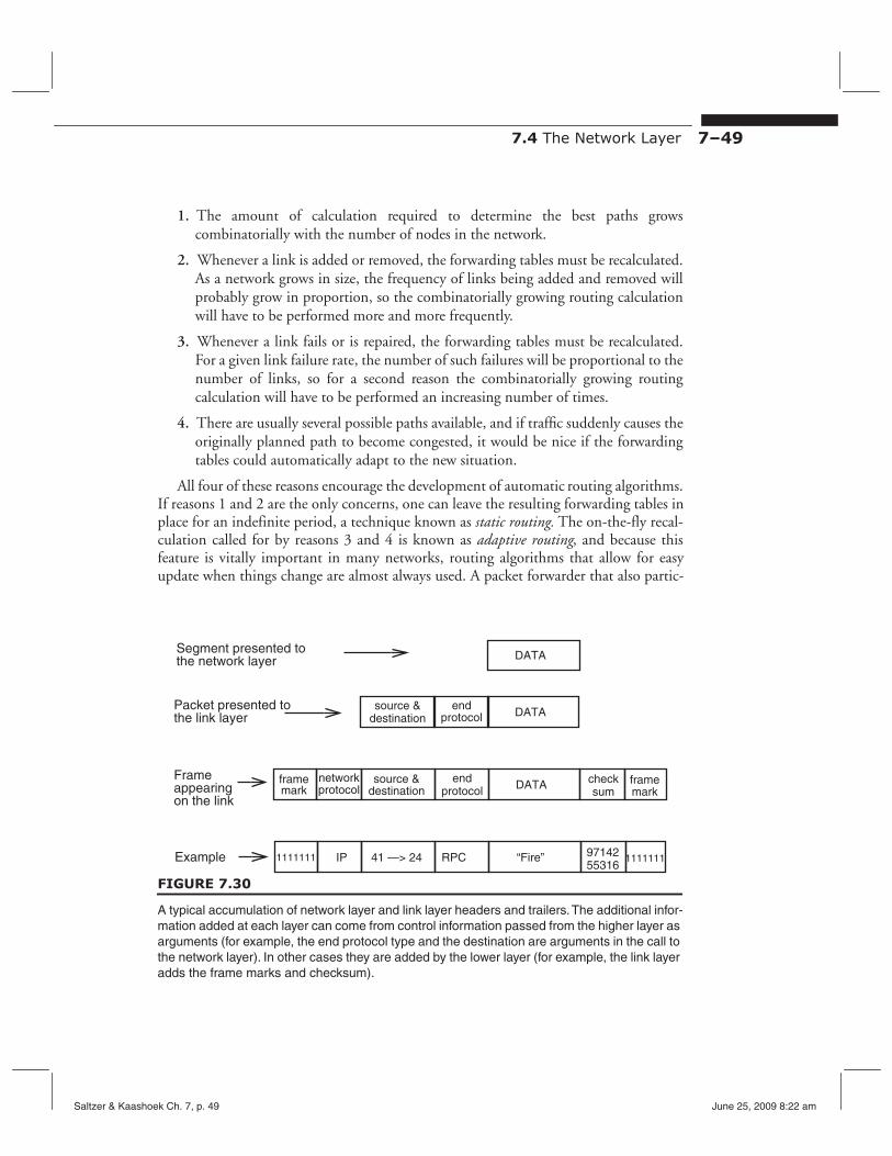
7.4 The Network Layer 7–49
1. The amount of calculation required to determine the best paths grows combinatorially with the number of nodes in the network.
2. Whenever a link is added or removed, the forwarding tables must be recalculated. As a network grows in size, the frequency of links being added and removed will probably grow in proportion, so the combinatorially growing routing calculation will have to be performed more and more frequently.
3. Whenever a link fails or is repaired, the forwarding tables must be recalculated. For a given link failure rate, the number of such failures will be proportional to the number of links, so for a second reason the combinatorially growing routing calculation will have to be performed an increasing number of times.
4. There are usually several possible paths available, and if traffic suddenly causes the originally planned path to become congested, it would be nice if the forwarding tables could automatically adapt to the new situation.
All four of these reasons encourage the development of automatic routing algorithms. If reasons 1 and 2 are the only concerns, one can leave the resulting forwarding tables in place for an indefinite period, a technique known as static routing. The on-the-fly recalculation called for by reasons 3 and 4 is known as adaptive routing, and because this feature is vitally important in many networks, routing algorithms that allow for easy update when things change are almost always used. A packet forwarder that also partic-
Segment presented to DATAthe network layer
Packet presented to the link layer DATAend
protocol source &
destination
frame check frameDATAend protocol
Frame appearing on the link
source & destination sum
network protocol
1111111 97142 1111111“Fire”RPCExample 41 —> 24 55316
IP
mark mark
FIGURE 7.30
A typical accumulation of network layer and link layer headers and trailers. The additional information added at each layer can come from control information passed from the higher layer as arguments (for example, the end protocol type and the destination are arguments in the call to the network layer). In other cases they are added by the lower layer (for example, the link layer adds the frame marks and checksum).
Saltzer & Kaashoek Ch. 7, p. 49 June 25, 2009 8:22 am
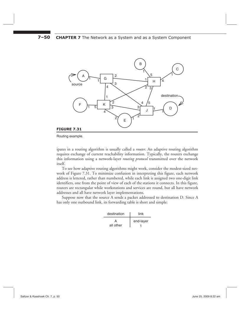
7–50 CHAPTER 7 The Network as a System and as a System Component
FIGURE 7.31
Routing example.
G
K
J
source 1
2 3
A
B
C
D
E
F
4
5
3 4 5
1
2
1 2
3 4
1
2 35
1
1
1 1
1
12
4
H
destination
ipates in a routing algorithm is usually called a router. An adaptive routing algorithm requires exchange of current reachability information. Typically, the routers exchange this information using a network-layer routing protocol transmitted over the network itself.
To see how adaptive routing algorithms might work, consider the modest-sized network of Figure 7.31. To minimize confusion in interpreting this figure, each network address is lettered, rather than numbered, while each link is assigned two one-digit link identifiers, one from the point of view of each of the stations it connects. In this figure, routers are rectangular while workstations and services are round, but all have network addresses and all have network layer implementations.
Suppose now that the source A sends a packet addressed to destination D. Since A has only one outbound link, its forwarding table is short and simple:
destination link
A end-layer all other 1
Saltzer & Kaashoek Ch. 7, p. 50 June 25, 2009 8:22 am
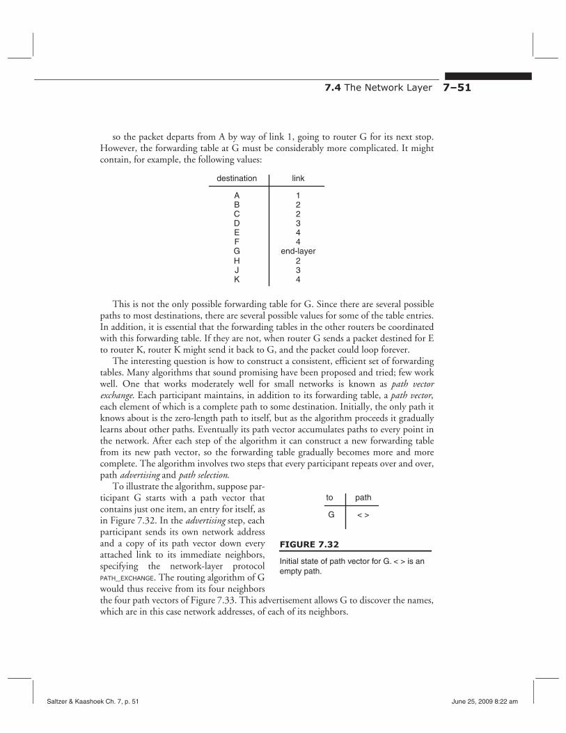
7.4 The Network Layer 7–51
so the packet departs from A by way of link 1, going to router G for its next stop. However, the forwarding table at G must be considerably more complicated. It might contain, for example, the following values:
destination link
A 1 B 2 C 2 D 3 E 4 F 4 G end-layer H 2 J 3 K 4
This is not the only possible forwarding table for G. Since there are several possible paths to most destinations, there are several possible values for some of the table entries. In addition, it is essential that the forwarding tables in the other routers be coordinated with this forwarding table. If they are not, when router G sends a packet destined for E to router K, router K might send it back to G, and the packet could loop forever.
The interesting question is how to construct a consistent, efficient set of forwarding tables. Many algorithms that sound promising have been proposed and tried; few work well. One that works moderately well for small networks is known as path vector exchange. Each participant maintains, in addition to its forwarding table, a path vector, each element of which is a complete path to some destination. Initially, the only path it knows about is the zero-length path to itself, but as the algorithm proceeds it gradually learns about other paths. Eventually its path vector accumulates paths to every point in the network. After each step of the algorithm it can construct a new forwarding table from its new path vector, so the forwarding table gradually becomes more and more complete. The algorithm involves two steps that every participant repeats over and over, path advertising and path selection.
To illustrate the algorithm, suppose participant G starts with a path vector that to contains just one item, an entry for itself, as
Gin Figure 7.32. In the advertising step, each participant sends its own network address and a copy of its path vector down every FIGURE 7.32 attached link to its immediate neighbors,
path
< >
specifying the network-layer protocol Initial state of path vector for G. < > is an empty path.
PATH_EXCHANGE. The routing algorithm of G would thus receive from its four neighbors the four path vectors of Figure 7.33. This advertisement allows G to discover the names, which are in this case network addresses, of each of its neighbors.
Saltzer & Kaashoek Ch. 7, p. 51 June 25, 2009 8:22 am
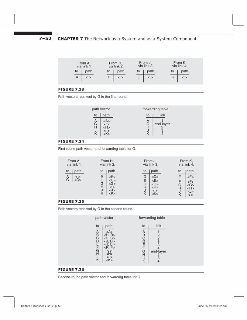
7–52 CHAPTER 7 The Network as a System and as a System Component
From A, From H, From J, From K,
to path
A < >
to path
H < >
to path
J < >
to path
K < >
via link 1 via link 2: via link 3: via link 4:
FIGURE 7.33
Path vectors received by G in the first round.
to path
A <A>
to link
A 1 G H J K
end-layer2 3 4
forwarding tablepath vector
G < > H J K
<H> <J> <K>
FIGURE 7.34
First-round path vector and forwarding table for G.
to path
A < > G <G>
to path
B <B>
G <G> H J K
< > <J> <K>
to path
F <F> G <G> H J K
<H> <J> < >
to path
D <D>
G <G> H J K
<H> < > <K>
From A, From H, From J, From K, via link 1 via link 2: via link 3: via link 4:
C <C> E <E>
E <E>
FIGURE 7.35
Path vectors received by G in the second round.
to path
A <A>
to link
A 1
G H J K
end-layer2 3 4
forwarding tablepath vector
G < > H J K
<H> <J> <K>
B C D E
B C D E F F
<H, B><H, C> <J, D><J, E> <K, F>
2 2 3 3 4
FIGURE 7.36
Second-round path vector and forwarding table for G.
Saltzer & Kaashoek Ch. 7, p. 52 June 25, 2009 8:22 am
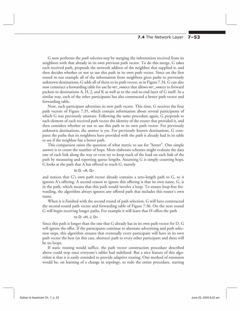
7.4 The Network Layer 7–53
G now performs the path selection step by merging the information received from its neighbors with that already in its own previous path vector. To do this merge, G takes each received path, prepends the network address of the neighbor that supplied it, and then decides whether or not to use this path in its own path vector. Since on the first round in our example all of the information from neighbors gives paths to previously unknown destinations, G adds all of them to its path vector, as in Figure 7.34. G can also now construct a forwarding table for use by NET_HANDLE that allows NET_HANDLE to forward packets to destinations A, H, J, and K as well as to the end-to-end layer of G itself. In a similar way, each of the other participants has also constructed a better path vector and forwarding table.
Now, each participant advertises its new path vector. This time, G receives the four path vectors of Figure 7.35, which contain information about several participants of which G was previously unaware. Following the same procedure again, G prepends to each element of each received path vector the identity of the router that provided it, and then considers whether or not to use this path in its own path vector. For previously unknown destinations, the answer is yes. For previously known destinations, G compares the paths that its neighbors have provided with the path it already had in its table to see if the neighbor has a better path.
This comparison raises the question of what metric to use for “better”. One simple answer is to count the number of hops. More elaborate schemes might evaluate the data rate of each link along the way or even try to keep track of the load on each link of the path by measuring and reporting queue lengths. Assuming G is simply counting hops, G looks at the path that A has offered to reach G, namely
to G: <A, G>
and notices that G’s own path vector already contains a zero-length path to G, so it ignores A’s offering. A second reason to ignore this offering is that its own name, G, is in the path, which means that this path would involve a loop. To ensure loop-free forwarding, the algorithm always ignores any offered path that includes this router’s own name.
When it is finished with the second round of path selection, G will have constructed the second-round path vector and forwarding table of Figure 7.36. On the next round G will begin receiving longer paths. For example it will learn that H offers the path
to D: <H, J, D>
Since this path is longer than the one that G already has in its own path vector for D, G will ignore the offer. If the participants continue to alternate advertising and path selection steps, this algorithm ensures that eventually every participant will have in its own path vector the best (in this case, shortest) path to every other participant and there will be no loops.
If static routing would suffice, the path vector construction procedure described above could stop once everyone’s tables had stabilized. But a nice feature of this algorithm is that it is easily extended to provide adaptive routing. One method of extension would be, on learning of a change in topology, to redo the entire procedure, starting
Saltzer & Kaashoek Ch. 7, p. 53 June 25, 2009 8:22 am
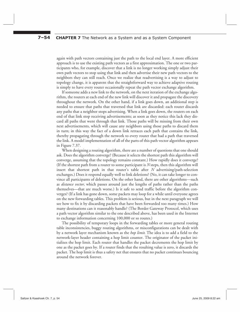
7–54 CHAPTER 7 The Network as a System and as a System Component
again with path vectors containing just the path to the local end layer. A more efficient approach is to use the existing path vectors as a first approximation. The one or two participants who, for example, discover that a link is no longer working simply adjust their own path vectors to stop using that link and then advertise their new path vectors to the neighbors they can still reach. Once we realize that readvertising is a way to adjust to topology change, it is apparent that the straightforward way to achieve adaptive routing is simply to have every router occasionally repeat the path vector exchange algorithm.
If someone adds a new link to the network, on the next iteration of the exchange algorithm, the routers at each end of the new link will discover it and propagate the discovery throughout the network. On the other hand, if a link goes down, an additional step is needed to ensure that paths that traversed that link are discarded: each router discards any paths that a neighbor stops advertising. When a link goes down, the routers on each end of that link stop receiving advertisements; as soon as they notice this lack they discard all paths that went through that link. Those paths will be missing from their own next advertisements, which will cause any neighbors using those paths to discard them in turn; in this way the fact of a down link retraces each path that contains the link, thereby propagating through the network to every router that had a path that traversed the link. A model implementation of all of the parts of this path vector algorithm appears in Figure 7.37.
When designing a routing algorithm, there are a number of questions that one should ask. Does the algorithm converge? (Because it selects the shortest path this algorithm will converge, assuming that the topology remains constant.) How rapidly does it converge? (If the shortest path from a router to some participant is N steps, then this algorithm will insert that shortest path in that router’s table after N advertising/path-selection exchanges.) Does it respond equally well to link deletions? (No, it can take longer to convince all participants of deletions. On the other hand, there are other algorithms—such as distance vector, which passes around just the lengths of paths rather than the paths themselves—that are much worse.) Is it safe to send traffic before the algorithm converges? (If a link has gone down, some packets may loop for a while until everyone agrees on the new forwarding tables. This problem is serious, but in the next paragraph we will see how to fix it by discarding packets that have been forwarded too many times.) How many destinations can it reasonably handle? (The Border Gateway Protocol, which uses a path vector algorithm similar to the one described above, has been used in the Internet to exchange information concerning 100,000 or so routes.)
The possibility of temporary loops in the forwarding tables or more general routing table inconsistencies, buggy routing algorithms, or misconfigurations can be dealt with by a network layer mechanism known as the hop limit. The idea is to add a field to the network-layer header containing a hop limit counter. The originator of the packet initializes the hop limit. Each router that handles the packet decrements the hop limit by one as the packet goes by. If a router finds that the resulting value is zero, it discards the packet. The hop limit is thus a safety net that ensures that no packet continues bouncing around the network forever.
Saltzer & Kaashoek Ch. 7, p. 54 June 25, 2009 8:22 am

7.4 The Network Layer 7–55
FIGURE 7.37
// Maintain routing and forwarding tables.
vector associative array // vector[d_addr] contains path to destination d_addr neighbor_vector instance of vector // A path vector received from some neighbor my_vector instance of vector // My current path vector. addr associative array // addr[j] is the address of the network attachment
// point at the other end of link j. // my_addr is address of my network attachment point. // A path is a parsable list of addresses, e.g. {a,b,c,d}
procedure main() // Initialize, then start advertising. SET_TYPE_HANDLER (HANDLE_ADVERTISEMENT, exchange_protocol) clear my_vector; // Listen for advertisements do occasionally // and advertise my paths
for each j in link_ids do // to all of my neighbors. status ← SEND_PATH_VECTOR (j, my_addr, my_vector, exch_protocol) if status ≠ 0 then // If the link was down,
clear new_vector // forget about any paths FLUSH_AND_REBUILD (j) // that start with that link.
procedure HANDLE_ADVERTISEMENT (advt, link_id) // Called when an advt arrives. addr[link_id] ← GET_SOURCE (advt) // Extract neighbor’s address neighbor_vector ← GET_PATH_VECTOR (advt) // and path vector. for each neighbor_vector.d_addr do // Look for better paths.
new_path ←{addr[link_id], neighbor_vector[d_addr]} // Build potential path. if my_addr is not in new_path then // Skip it if I’m in it.
if my_vector[d_addr] = NULL) then // Is it a new destination? my_vector[d_addr] ← new_path // Yes, add this one.
else // Not new; if better, use it. my_vector[d_addr] ← SELECT_PATH (new_path, my_vector[d_addr])
FLUSH_AND_REBUILD (link_id)
procedure SELECT_PATH (new, old) // Decide if new path is better than old one. if first_hop(new) = first_hop(old) then return new // Update any path we were
// already using. else if length(new) ≥ length(old) then return old // We know a shorter path, keep else return new // OK, the new one looks better.
procedure FLUSH_AND_REBUILD (link_id) // Flush out stale paths from this neighbor. for each d_addr in my_vector
if first_hop(my_vector[d_addr]) = addr[link_id] and new_vector[d_addr] = NULL
then delete my_vector[d_addr] // Delete paths that are no longer advertised.
REBUILD_FORWARDING_TABLE (my_vector, addr) // Pass info to forwarder.
Model implementation of a path vector exchange routing algorithm. These procedures run in every participating router. They assume that the link layer discards damaged packets. If an advertisement is lost, it is of little consequence because the next advertisement will replace it The procedure REBUILD_FORWARDING_TABLE is not shown; it simply constructs a new forwarding table for use by this router, using the latest path vector information.
Saltzer & Kaashoek Ch. 7, p. 55 June 25, 2009 8:22 am
7–56 CHAPTER 7 The Network as a System and as a System Component
There are some obvious refinements that can be made to the path vector algorithm. For example, since nodes such as A, B, C, D, and F are connected by only one link to the rest of the network, they can skip the path selection step and just assume that all destinations are reachable via their one link—but when they first join the network they must do an advertising step, to ensure that the rest of the network knows how to reach them (and it would be wise to occasionally repeat the advertising step, to make sure that link failures and router restarts don’t cause them to be forgotten). A service node such as E, which has two links to the network but is not intended to be used for transit traffic, may decide never to advertise anything more than the path to itself. Because each participant can independently decide which paths it advertises, path vector exchange is sometimes used to implement restrictive routing policies. For example, a country might decide that packets that both originate and terminate domestically should not be allowed to transit another country, even if that country advertises a shorter path.
The exchange of data among routers is just another example of a network layer protocol. Since the link layer already provides network layer protocol multiplexing, no extra effort is needed to add a routing protocol to the layered system. Further, there is nothing preventing different groups of routers from choosing to use different routing protocols among themselves. In the Internet, there are many different routing protocols simultaneously in use, and it is common for a single router to use different routing protocols over different links.
7.4.3 Hierarchical Address Assignment and Hierarchical Routing
The system for identifying attachment points of a network as described so far is workable, but does not scale up well to large numbers of attachment points. There are two immediate problems:
1. Every attachment point must have a unique address. If there are just ten attachment points, all located in the same room, coming up with a unique identifier for an eleventh is not difficult. But if there are several hundred million attachment points in locations around the world, as in the Internet, it is hard to maintain a complete and accurate list of addresses already assigned.
2. The path vector grows in size with the number of attachment points. Again, for routers to exchange a path vector with ten entries is not a problem; a path vector with 100 million entries could be a hassle.
The usual way to tackle these two problems is to introduce hierarchy: invent some scheme by which network addresses have a hierarchical structure that we can take advantage of, both for decentralizing address assignments and for reducing the size of forwarding tables and path vectors.
For example, consider again the abstract network of Figure 7.28, in which we arbitrarily assigned two-digit numbers as network addresses. Suppose we instead adopt a more structured network address consisting, say, of two parts, which we might call
Saltzer & Kaashoek Ch. 7, p. 56 June 25, 2009 8:22 am
7.4 The Network Layer 7–57
“region” and “station”. Thus in Figure 7.31 we might assign to A the network address “11,75” where 11 is a region identifier and 75 is a station identifier.
By itself, this change merely complicates things. However, if we also adopt a policy that regions must correspond to the set of network attachment points served by an identifiable group of closely-connected routers, we have a lever that we can use to reduce the size of forwarding tables and path vectors. Whenever a router for region 11 gets ready to advertise its path vector to a router that serves region 12, it can condense all of the paths for the region 11 network destinations it knows about into a single path, and simply advertise that it knows how to forward things to any region 11 network destination. The routers that serve region 11 must, of course, still maintain complete path vectors for every region 11 station, and exchange those vectors among themselves, but these vectors are now proportional in size to the number of attachment points in region 11, rather than to the number of attachment points in the whole network.
When a network uses hierarchical addresses, the operation of forwarding involves the same steps as before, but the table lookup process is slightly more complicated: The forwarder must first extract the region component of the destination address and look that up in its forwarding table. This lookup has two possible outcomes: either the forwarding table contains an entry showing a link over which to send the packet to that region, or the forwarding table contains an entry saying that this forwarder is already in the destination region, in which case it is necessary to extract the station identifier from the destination address and look that up in a distinct part of the forwarding table. In most implementations, the structure of the forwarding table reflects the hierarchical structure of network addresses. Figure 7.38 illustrates the use of a forwarding table for hierarchical addresses that is constructed of two sections.
Hierarchical addresses also offer an opportunity to grapple with the problem of assigning unique addresses in a large network because the station part of a network address needs to be unique only within its region. A central authority can assign region identifiers, while different local authorities can assign the station identifiers within each region, without consulting other regional authorities. For this decentralization to work, the boundaries of each local administrative authority must coincide with the boundaries of the regions served by the packet forwarders. While this seems like a simple thing to arrange, it can actually be problematic. One easy way to define regions of closely connected packet forwarders is to do it geographically. However, administrative authority is often not organized on a strictly geographic basis. So there may be a significant tension between the needs of address assignment and the needs of packet forwarding.
Hierarchical network addresses are not a panacea—in addition to complexity, they introduce at least two new problems. With the non-hierarchical scheme, the geographical location of a network attachment point did not matter, so a portable computer could, for example, connect to the network in either Boston or San Francisco, announce its network address, and after the routers have exchanged path vectors a few times, expect to communicate with its peers. But with hierarchical routing, this feature stops working. When a portable computer attaches to the network in a different region, it cannot simply advertise the same network address that it had in its old region. It will instead have to
Saltzer & Kaashoek Ch. 7, p. 57 June 25, 2009 8:22 am
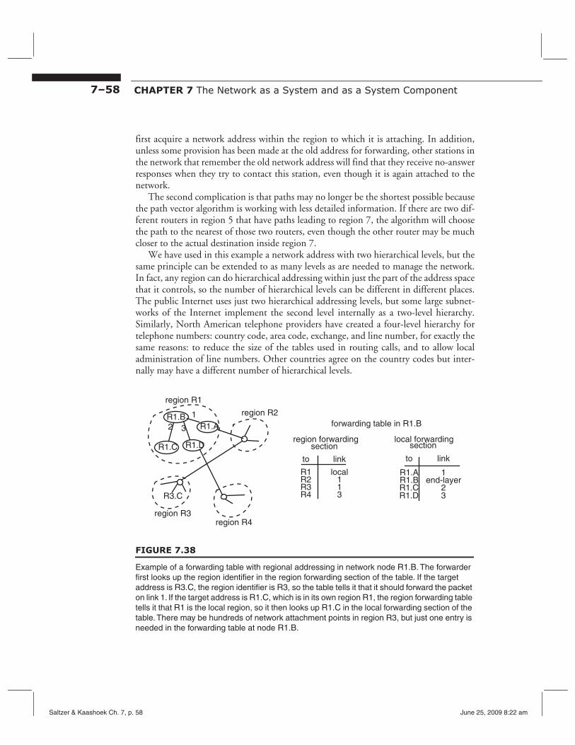
7–58 CHAPTER 7 The Network as a System and as a System Component
first acquire a network address within the region to which it is attaching. In addition, unless some provision has been made at the old address for forwarding, other stations in the network that remember the old network address will find that they receive no-answer responses when they try to contact this station, even though it is again attached to the network.
The second complication is that paths may no longer be the shortest possible because the path vector algorithm is working with less detailed information. If there are two different routers in region 5 that have paths leading to region 7, the algorithm will choose the path to the nearest of those two routers, even though the other router may be much closer to the actual destination inside region 7.
We have used in this example a network address with two hierarchical levels, but the same principle can be extended to as many levels as are needed to manage the network. In fact, any region can do hierarchical addressing within just the part of the address space that it controls, so the number of hierarchical levels can be different in different places. The public Internet uses just two hierarchical addressing levels, but some large subnetworks of the Internet implement the second level internally as a two-level hierarchy. Similarly, North American telephone providers have created a four-level hierarchy for telephone numbers: country code, area code, exchange, and line number, for exactly the same reasons: to reduce the size of the tables used in routing calls, and to allow local administration of line numbers. Other countries agree on the country codes but internally may have a different number of hierarchical levels.
region R1
to link
R1.A 1
forwarding table in R1.B
R1.B R1.C
end-layer2
to link
R1 local R2 R3 R4
1 1 3
region forwarding local forwarding
region R2
region R3
R1.B
R3.C
R1.C
1
32 R1.A
R1.D 3
R1.D section section
region R4
FIGURE 7.38
Example of a forwarding table with regional addressing in network node R1.B. The forwarder first looks up the region identifier in the region forwarding section of the table. If the target address is R3.C, the region identifier is R3, so the table tells it that it should forward the packet on link 1. If the target address is R1.C, which is in its own region R1, the region forwarding table tells it that R1 is the local region, so it then looks up R1.C in the local forwarding section of the table. There may be hundreds of network attachment points in region R3, but just one entry is needed in the forwarding table at node R1.B.
Saltzer & Kaashoek Ch. 7, p. 58 June 25, 2009 8:22 am

7.4 The Network Layer 7–59
7.4.4 Reporting Network Layer Errors
The network layer can encounter trouble when trying to forward a packet, so it needs a way of reporting that trouble. The network layer is in a uniquely awkward position when this happens because the usual reporting method (return a status value to the higher-layer program that asked for this operation) may not be available. An intermediate router receives a packet from a link layer below, and it is expected to forward that packet via another link layer. Even if there is a higher layer in the router, that layer probably has no interest in this packet. Instead, the entity that needs to hear about the problem is more likely to be the upper layer program that originated the packet, and that program may be located several hops away in another computer. Even the network layer at the destination address may need to report something to the original sender such as the lack of an upper-layer handler for the end-to-end type that the sender specified.
The obvious thing to do is send a message to the entity that needs to know about the problem. The usual method is that the network layer of the router creates a new packet on the spot and sends it back to the source address shown in the problem packet. The message in this new packet reports details of the problem using some standard error reporting protocol. With this design, the original higher-layer sender of a packet is expected to listen not only for replies but also for messages of the error reporting protocol. Here are some typical error reports:
• The buffers of the router were full, so the packet had to be discarded. • The buffers of the router are getting full—please stop sending so many packets. • The region identifier part of the target address does not exist. • The station identifier part of the target address does not exist. • The end type identifier was not recognized. • The packet is larger than the maximum transmission unit of the next link. • The packet hop limit has been exceeded.
In addition, a copy of the header of the doomed packet goes into a data field of the error message, so that the recipient can match it with an outstanding SEND request.
One might suggest that a router send an error report when discarding a packet that is received with a wrong checksum. This idea is not as good as it sounds because a damaged packet may have garbled header information, in which case the error message might be sent to a wrong—or even nonexistent—place. Once a packet has been identified as containing unknown damage, it is not a good idea to take any action that depends on its contents.
A network-layer error reporting protocol is a bit unusual. An error message originates in the network layer, but is delivered to the end-to-end layer. Since it crosses layers, it can be seen as violating (in a minor way) the usual separation of layers: we have a network layer program preparing an end-to-end header and inserting end-to-end data; a strict layer doctrine would insist that the network layer not touch anything but network layer headers.
Saltzer & Kaashoek Ch. 7, p. 59 June 25, 2009 8:22 am
7–60 CHAPTER 7 The Network as a System and as a System Component
An error reporting protocol is usually specified to be a best-effort protocol, rather than one that takes heroic efforts to get the message through. There are two reasons why this design decision makes sense. First, as will be seen in Section 7.5 of this chapter, implementing a more reliable protocol adds a fair amount of machinery: timers, keeping copies of messages in case they need to be retransmitted, and watching for receipt acknowledgments. The network layer is not usually equipped to do any of these functions, and not implementing them minimizes the violation of layer separation. Second, error messages can be thought of as hints that allow the originator of a packet to more quickly discover a problem. If an error message gets lost, the originator should, one way or another, eventually discover the problem in some other way, perhaps after timing out, resending the original packet, and getting an error message on the retry.
A good example of the best-effort nature of an error reporting protocol is that it is common to not send an error message about every discarded packet; if congestion is causing the discard rate to climb, that is exactly the wrong time to increase the network load by sending many “I discarded your packet” notices. But sending a few such notices can help alert sources who are flooding the network that they need to back off—this topic is explored in more depth in Section 7.6.
The basic idea of an error reporting protocol can be used for other communications to and from the network layer of any participant in the network. For example, the Internet has a protocol named internet control message protocol (ICMP) that includes an echo request message (also known as a “ping,” from an analogy with submarine active sonar systems). If an end node sends an echo request to any network participant, whether a packet forwarder or another end node, the network layer in that participant is expected to respond by immediately sending the data of the message back to the sender in an echo reply message. Echo request/reply messages are widely used to determine whether or not a participant is actually up and running. They are also sometimes used to assess network congestion by measuring the time until the reply comes back.
Another useful network error report is “hop limit exceeded”. Recall from page 7–54 that to provide a safety net against the possibility of forwarding loops, a packet may contain a hop limit field, which a router decrements in each packet that it forwards. If a router finds that the hop limit field contains zero, it discards the packet and it also sends back a message containing the error report. The “hop limit exceeded” error message provides feedback to the originator, for example it may have chosen a hop limit that is too small for the network configuration. The “hop limit exceeded” error message can also be used in an interesting way to help locate network problems: send a test message (usually called a probe) to some distant destination address, but with the hop limit set to 1. This probe will cause the first router that sees it to send back a “hop limit exceeded” message whose source address identifies that first router. Repeat the experiment, sending probes with hop limits set to 2, 3,…, etc. Each response will reveal the network address of the next router along the current path between the source and the destination. In addition, the time required for the response to return gives a rough indication of the network load between the source and that router. In this way one can trace the current path through the network to the destination address, and identify points of congestion.
Saltzer & Kaashoek Ch. 7, p. 60 June 25, 2009 8:22 am
7.4 The Network Layer 7–61
Another way to use an error reporting protocol is for the end-to-end layer to send a series of probes to learn the smallest maximum transmission unit (MTU) that lies on the current path between it and another network attachment point. It first sends a packet of the largest size the application has in mind. If this probe results in an “MTU exceeded” error response, it halves the packet size and tries again. A continued binary search will quickly home in on the smallest MTU along the path. This procedure is known as MTU discovery.
7.4.5 Network Address Translation (An Idea That Almost Works)
From a naming point of view, the Internet provides a layered naming environment with two contexts for its network attachment points, known as “Internet addresses”. An Internet address has two components, a network number and a host number. Most network numbers are global names, but a few, such as network 10, are designated for use in private networks. These network numbers can be used either completely privately, or in conjunction with the public Internet. Completely private use involves setting up an independent private network, and assigning host addresses using the network number 10. Routers within this network advertise and forward just as in the public Internet. Routers on the public Internet follow the convention that they do not accept routes to network 10, so if this private network is also directly attached to the public Internet, there is no confusion. Assuming that the private network accepts routes to globally named networks, a host inside the private network could send a message to a host on the public Internet, but a host on the public Internet cannot send a response back because of the routing convention. Thus any number of private networks can each independently assign numbers using network number 10—but hosts on different private networks cannot talk to one another and hosts on the public Internet cannot talk to them.
Network Address Translation (NAT) is a scheme to bridge this gap. The idea is that a specialized translating router (known informally as a “NAT box”) stands at the border between a private network and the public Internet. When a host inside the private network wishes to communicate with a service on the public Internet, it first makes a request to the translating router. The translator sets up a binding between that host’s private address and a temporarily assigned public address, which the translator advertises to the public Internet. The private host then launches a packet that has a destination address in the public Internet, and its own private network source address. As this packet passes through the translating router, the translator modifies the source address by replacing it with the temporarily assigned public address. It then sends the packet on its way into the public Internet. When a response from the service on the public Internet comes back to the translating router, the translator extracts the destination address from the response, looks it up in its table of temporarily assigned public addresses, finds the internal address to which it corresponds, modifies the destination address in the packet, and sends the packet on its way on the internal network, where it finds its way to the private host that initiated the communication.
Saltzer & Kaashoek Ch. 7, p. 61 June 25, 2009 8:22 am
7–62 CHAPTER 7 The Network as a System and as a System Component
The scheme works, after a fashion, but it has a number of limitations. The most severe limitation is that some end-to-end network protocols place Internet addresses in fields buried in their payloads; there is nothing restricting Internet addresses to packet source and destination fields of the network layer header. For example, some protocols between two parties start by mentioning the Internet address of a third party, such as a bank, that must also participate in the protocol. If the Internet address of the third party is on the public Internet, there may be no problem, but if it is an address on the private network, the translator needs to translate it as it goes by. The trouble is that translation requires that the translator peer into the payload data of the packet and understand the format of the higher-layer protocol. The result is that NAT works only for those protocols that the translator is programmed to understand. Some protocols may present great difficulties. For example, if a secure protocol uses key-driven cryptographic transformations for either privacy or authentication, the NAT gateway would need to have a copy of the keys, but giving it the keys may defeat the purpose of the secure protocol. (This concern will become clearer after reading Chapter 11[on-line].)
A second problem is that all of the packets between the public Internet and the private network must pass through the translating router, since it is the only place that knows how to do the address translation. The translator thus introduces both a potential bottleneck and a potential single point of failure, and NAT becomes a constraint on routing policy.
A third problem arises if two such organizations later merge. Each organization will have assigned addresses in network 10, but since their assignments were not coordinated, some addresses will probably have been assigned in both organizations, and all of the colliding addresses must be discovered and changed.
Although originally devised as a scheme to interconnect private networks to the public Internet, NAT has become popular as a technique to beef up security of computer systems that have insecure operating system or network implementations. In this application, the NAT translator inspects every packet coming from the public Internet and refuses to pass along any whose origin seems suspicious or that try to invoke services that are not intended for public use. The scheme does not in itself provide much security, but in conjunction with other security mechanisms described in Chapter 11[on-line], it can help create what that chapter describes as “defense in depth”.
7.5 The End-to-End Layer The network layer provides a useful but not completely dependable best-effort communication environment that will deliver data segments to any destination, but with no guarantees about delay, order of arrival, certainty of arrival, accuracy of content, or even of delivery to the right place. This environment is too hostile for most applications, and the job of the end-to-end layer is to create a more comfortable communication environment that has the features of performance, reliability, and certainty that an application needs. The complication is that different applications can have quite different commu-
Saltzer & Kaashoek Ch. 7, p. 62 June 25, 2009 8:22 am
7.5 The End-to-End Layer 7–63
nication needs, so no single end-to-end design is likely to suffice. At the same time, applications tend to fall in classes all of whose members have somewhat similar requirements. For each such class it is usually possible to design a broadly useful protocol, known as a transport protocol, for use by all the members of the class.
7.5.1 Transport Protocols and Protocol Multiplexing
A transport protocol operates between two attachment points of a network, with the goal of moving either messages or a stream of data between those points while providing a particular set of specified assurances. As was explained in Chapter 4, it is convenient to distinguish the two attachment points by referring to the application program that initiates action as the client and the application program that responds as the service. At the same time, data may flow either from client to service, from service to client, or both, so we will need to refer to the sending and receiving sides for each message or stream. Transport protocols almost always include multiplexing, to tell the receiving side to which application it should deliver the message or direct the stream. Because the mechanics of application multiplexing can be more intricate than in lower layers, we first describe a transport protocol interface that omits multiplexing, and then add multiplexing to the interface.
In contrast with the network layer, where an important feature is a uniform application programming interface, the interface to an end-to-end transport protocol varies with the particular end-to-end semantics that the protocol provides. Thus a simple message-sending protocol that is intended to be used by only one application might have a first-version interface such as:
v.1 SEND_MESSAGE (destination, message)
in which, in addition to supplying the content of the message, the sender specifies in des
tination the network attachment point to which the message should be delivered. The sender of a message needs to know both the message format that the recipient expects and the destination address. Chapter 3 described several methods of discovering destination addresses, any of which might be used.
The prospective receiver must provide an interface by which the transport protocol delivers the message to the application. Just as in the link and network layers, receiving a message can’t happen until the message arrives, so receiving involves waiting and the corresponding receive-side interface depends on the system mechanisms that are available for waiting and for thread or event coordination. For illustration, we again use an upcall: when a message arrives, the message transport protocol delivers it by calling an application-provided procedure entry point:
V.1 DELIVER_MESSAGE (message)
This first version of an upcall interface omits not only multiplexing but another important requirement: When sending a message, the sender usually expects a reply. While a programmer may be able to ask someone down the hall the appropriate destination address to use for some service, it is usually the case that a service has many clients. Thus
Saltzer & Kaashoek Ch. 7, p. 63 June 25, 2009 8:22 am
7–64 CHAPTER 7 The Network as a System and as a System Component
the service needs to know where each message came from so that it can send a reply. A message transport protocol usually provides this information, for example by including a second argument in the upcall interface:
V.2 DELIVER_MESSAGE (source, message)
In this second (but not quite final) version of the upcall, the transport protocol sets the value of source to the address from which this message originated. The transport protocol obtains the value of source as an argument of an upcall from the network layer.
Since the reason for designing a message transport protocol is that it is expected to be useful to several applications, the interface needs additional information to allow the protocol to know which messages belong to which application. End-to-end layer multiplexing is generally a bit more complicated than that of lower layers because not only can there be multiple applications, there can be multiple instances of the same application using the same transport protocol. Rather than assigning a single multiplexing identifier to an application, each instance of an application receives a distinct multiplexing identifier, usually known as a port. In a client/service situation, most application services advertise one of these identifiers, called that application’s well-known port. Thus the second (and again not final) version of the send interface is
v.2SEND_MESSAGE (destination, service_port, message)
where service_port identifies the well-known port of the application service to which the sender wants to have the message delivered. At the receiving side each application that expects to receive messages needs to tell the message transport protocol what port it expects clients to use, and it must also tell the protocol what program to call to deliver messages. The application can provide both pieces of information invoking the transport protocol procedure
LISTEN_FOR_MESSAGES (service_port, message_handler)
which alerts the transport protocol implementation that whenever a message arrives at this destination carrying the port identifier service_port, the protocol should deliver it by calling the procedure named in the second argument (that is, the procedure message_handler). LISTEN_FOR_MESSAGES enters its two arguments in a transport layer table for future reference. Later, when the transport protocol receives a message and is ready to deliver it, it invokes a dispatcher similar to that of Figure 7.27, on page 7–43. The dispatcher looks in the table for the service port that came with the message, identifies the associated message_handler procedure, and calls it, giving as arguments the source and the message.
One might expect that the service might send replies back to the client using the same application port number, but since one service might have several clients at the same network attachment point, each client instance will typically choose a distinct port number for its own replies, and the service needs to know to which port to send the reply. So the
Saltzer & Kaashoek Ch. 7, p. 64 June 25, 2009 8:22 am
7.5 The End-to-End Layer 7–65
SEND interface must be extended one final time to allow the sender to specify a port number to use for reply:
v.3 SEND_MESSAGE (destination, service_port, reply_port, message)
where reply_port is the identifier that the service can use to send a message back to this particular client. When the service does send its reply message, it may similarly specify a reply_port that is different from its well-known port if it expects that same client to send further, related messages. The reply_port arguments in the two directions thus allow a series of messages between a client and a service to be associated with one another.
Having added the port number to SEND_MESSAGE, we must communicate that port number to the recipient by adding an argument to the upcall by the message transport protocol when it delivers a message to the recipient:
v.3 DELIVER_MESSAGE (source, reply_port, message)
This third and final version of DELIVER_MESSAGE is the handler that the application designated when it called LISTEN_FOR_MESSAGES. The three arguments tell the handler (1) who sent the message (source), (2) the port on which that sender said it will listen for a possible reply (reply_port) and (3) the content of the message itself (message).
The interface set {LISTEN_FOR_MESSAGE, SEND_MESSAGE, DELIVER_MESSAGE} is specialized to end-to-end transport of discrete messages. Sidebar 7.5 illustrates two other, somewhat different, end-to-end transport protocol interfaces, one for a request/response protocol and the second for streams. Each different transport protocol can be thought of as a prepackaged set of improvements on the best-effort contract of the network layer. Here are three examples of transport protocols used widely in the Internet, and the assurances they provide:
1. User datagram protocol (UDP). This protocol adds ports for multiple applications and a checksum for data integrity to the network-layer packet. Although UDP is used directly for some simple request/reply applications such as asking for the time of day or looking up the network address of a service, its primary use is as a component of other message transport protocols, to provide end-to-end multiplexing and data integrity. [For details, see Internet standard STD0006 or Internet request for comments RFC–768.]
2. Transmission control protocol (TCP). Provides a stream of bytes with the assurances that data is delivered in the order it was originally sent, nothing is missing, nothing is duplicated, and the data has a modest (but not terribly high) probability of integrity. There is also provision for flow control, which means that the sender takes care not to overrun the ability of the receiver to accept data, and TCP cooperates with the network layer to avoid congestion. This protocol is used for applications such as interactive typing that require a telephone-like connection in which the order of delivery of data is important. (It is also used in many bulk transfer applications that do not require delivery order, but that do want to take advantage of its data integrity, flow control, and congestion avoidance assurances.)
Saltzer & Kaashoek Ch. 7, p. 65 June 25, 2009 8:22 am
7–66 CHAPTER 7 The Network as a System and as a System Component
Sidebar 7.5: Other end-to-end transport protocol interfaces Since there are many different combinations of services that an end-to-end transport protocol might provide, there are equally many transport protocol interfaces. Here are two more examples:
1. A request/response protocol sends a request message and waits for a response to that message before returning to the application. Since an interface that waits for a response ensures that there can be only one such call per thread outstanding, neither an explicit multiplexing parameter nor an upcall are necessary. A typical client interface to a request/response transport protocol is
response ← SEND_REQUEST (service_identifier, request)
where service_identifier is a name used by the transport protocol to locate the service destination and service port. It then sends a message, waits for a matching response, and delivers the result. The corresponding application programming interface at the service side of a request/response protocol may be equally simple or it can be quite complex, depending on the performance requirements.
2. A reliable message stream protocol sends several messages to the same destination with the intent that they be delivered reliably and in the order in which they were sent. There are many ways of defining a stream protocol interface. In the following example, an application client begins by creating a stream:
client_stream_id ← OPEN_STREAM (destination, service_port, reply_port)
followed by several invocations of:
WRITE_STREAM (client_stream_id, message)
and finally ends with:
CLOSE_STREAM (client_stream_id)
The service-side programming interface allows for several streams to be coming in to an application at the same time. The application starts by calling a LISTEN_FOR_STREAMS
procedure to post a listener on the service port, just as with the message interface. When a client opens a new stream, the service’s network layer, upon receiving the open request, upcalls to the stream listener that the application posted:
OPEN_STREAM_REQUEST (source, reply_port)
and upon receiving such an upcall OPEN_STREAM_REQUEST assigns a stream identifier for use within the service and invokes a transport layer dispatcher with
ACCEPT_STREAM (service_stream_id, next_message_handler)
The arrival of each message on the stream then leads the dispatcher to perform an upcall to the program identified in the variable next_message_handler:
HANDLE_NEXT_MESSAGE (stream_id, message);
With this design, a message value of NULL might signal that the client has closed the stream.
Saltzer & Kaashoek Ch. 7, p. 66 June 25, 2009 8:22 am
7.5 The End-to-End Layer 7–67
[For details, see Internet standard STD0007 or Internet request for comments RFC–793.]
3. Real-time transport protocol (RTP). Built on UDP (but with checksums switched off ), RTP provides a stream of time-stamped packets with no other integrity guarantee. This kind of protocol is useful for applications such as streaming video or voice, where order and stream timing are important, but an occasional lost packet is not a catastrophe, so out-of-order packets can be discarded, and packets with bits in error may still contain useful data. [For details, see Internet request for comments RFC–1889.]
There have, over the years, been several other transport protocols designed for use with the Internet, but they have not found enough application to be widely implemented. There are also several end-to-end protocols that provide services in addition to message transport, such as file transfer, file access, remote procedure call, and remote system management, and that are built using UDP or TCP as their underlying transport mechanism. These protocols are usually classified as presentation protocols because the primary additional service they provide is translating data formats between different computer platforms. This collection of protocols illustrates that the end-to-end layer is itself sometimes layered and sometimes not, depending on the requirements of the application.
Finally, end-to-end protocols can be multipoint, which means they involve more than two players. For example, to complete a purchase transaction, there may be a buyer, a seller, and one or more banks, each of which needs various end-to-end assurances about agreement, order of delivery, and data integrity.
In the next several sections, we explore techniques for providing various kinds of end-to-end assurances. Any of these techniques may be applied in the design of a message transport protocol, a presentation protocol, or by the application itself.
7.5.2 Assurance of At-Least-Once Delivery; the Role of Timers
A property of a best-effort network is that it may lose packets, so a goal of many end-toend transport protocols is to eliminate the resulting uncertainty about delivery. A persistent sender is a protocol participant that tries to ensure that at least one copy of each data segment is delivered, by sending it repeatedly until it receives an acknowledgment. The usual implementation of a persistent sender is to add to the application data a header containing a nonce and to set a timer that the designer estimates will expire in a little more than one network round-trip time, which is the sum of the network transit time for the outbound segment, the time the receiver spends absorbing the segment and preparing an acknowledgment, and the network transit time for the acknowledgment. Having set the timer, the sender passes the segment to the network layer for delivery, taking care to keep a copy. The receiving side of the protocol strips off the end-to-end header, passes the application data along to the application, and in addition sends back an acknowledgment that contains the nonce. When the acknowledgment gets back to the sender, the
Saltzer & Kaashoek Ch. 7, p. 67 June 25, 2009 8:22 am
7–68 CHAPTER 7 The Network as a System and as a System Component
sender uses the nonce to identify which previously-sent segment is being acknowledged. It then turns off the corresponding timer and discards its copy of that segment. If the timer expires before the acknowledgment returns, the sender restarts the timer and resends the segment, repeating this sequence indefinitely, until it receives an acknowledgment. For its part, the receiver sends back an acknowledgment every time it receives a segment, thereby extending the persistence in the reverse direction, thus covering the possibility that the best-effort network has lost one or more acknowledgments.
A protocol that includes a persistent sender does its best to provide an assurance of at-least-once delivery, which has semantics similar to the at-least-once RPC introducd in Section 4.2.2. The nonce, timer, retry, and acknowledgment together act to ensure that the data segment will eventually get through. As long as there is a non-zero probability of a message getting through, this protocol will eventually succeed. On the other hand, the probability may actually be zero, either for an indefinite time—perhaps the network is partitioned or the destination is not currently listening, or permanently—perhaps the destination is on a ship that has sunk. Because of the possibility that there will not be an acknowledgment forthcoming soon, or perhaps ever, a practical sender is not infinitely persistent. The sender limits the number of retries, and if the number exceeds the limit, the sender returns error status to the application that asked to send the message. The application must interpret this error status with some understanding of network communications. The lack of an acknowledgment means that one of two—significantly different—events has occurred:
1. The data segment was not delivered.
2. The data segment was delivered, but the acknowledgment never returned.
The good news is that the application is now aware that there is a problem. The bad news is that there is no way to determine which of the two problems occurred. This dilemma is intrinsic to communication systems, and the appropriate response depends on the particular application. Some applications will respond to this dilemma by making a note to later ask the other side whether or not it got the message; other applications may just ignore the problem. Chapter 10[on-line] investigates this issue further.
In summary, just as with at-least-once RPC, the at-least-once delivery protocol does not provide the absolute assurance that its name implies; it instead provides the assurance that if it is possible to get through, the message will get through, and if it is not possible to confirm delivery, the application will know about it.
The at-least-once delivery protocol provides no assurance about duplicates—it actually tends to generate duplicates. Furthermore, the assurance of delivery is weaker than appears on the surface: the data may have been corrupted along the way, or it may have been delivered to the wrong destination—and acknowledged—by mistake. Assurances on any of those points require additional techniques. Finally, the at-least-once delivery protocol ensures only that the message was delivered, not that the application actually acted on it—the receiving system may have been so overloaded that it ignored the message or it may have crashed an instant after acknowledging the message. When examining end-to-end assurances, it is important to identify the end points. In this case,
Saltzer & Kaashoek Ch. 7, p. 68 June 25, 2009 8:22 am
7.5 The End-to-End Layer 7–69
the receiving end point is the place in the protocol code that sends the acknowledgment of message receipt.
This protocol requires the sender to choose a value for the retry timer at the time it sends a packet. One possibility would be to choose in advance a timer value to be used for every packet—a fixed timer. But using a timer value fixed in advance is problematic because there is no good way to make that choice. To detect a lost packet by noticing that no acknowledgment has returned, the appropriate timer interval would be the expected network round-trip time plus some allowance for unusual queuing delays. But even the expected round-trip time between two given points can vary by quite a bit when routes change. In fact, one can argue that since the path to be followed and the amount of queuing to be tolerated is up to the network layer, and the individual transit times of links are properties of the link layer, for the end-to-end layer to choose a fixed value for the timer interval would violate the layering abstraction—it would require that the end-to-end layer know something about the internal implementation of the link and network layers.
Even if we are willing to ignore the abstraction concern, the end-to-end transport protocol designer has a dilemma in choosing a fixed timer interval. If the designer chooses too short an interval, there is a risk that the protocol will resend packets unnecessarily, which wastes network capacity as well as resources at both the sending and receiving ends. But if the designer sets the timer too long, then genuinely lost packets will take a long time to discover, so recovery will be delayed and overall performance will decline. Worse, setting a fixed value for a timer will not only force the designer to choose between these two evils, it will also embed in the system a lurking surprise that may emerge long in the future when someone else changes the system, for example to use a faster network connection. Going over old code to understand the rationale for setting the timers and choosing new values for them is a dismal activity that one would prefer to avoid by better design.
There are two common ways to minimize the use of fixed timers, both of which are applicable only when a transport protocol sends a stream of data segments to the same destination: adaptive timers and negative acknowledgments.
An adaptive timer is one whose setting dynamically adjusts to currently observed conditions. A common implementation scheme is to observe the round-trip times for each data segment and its corresponding response and calculate an exponentially weighted moving average of those measurements (Sidebar 7.6 explains the method). The protocol then sets its timers to, say, 150% of that estimate, with the intent that minor variations in queuing delay should rarely cause the timer to expire. Keeping an estimate of the round-trip time turns out to be useful for other purposes, too. An example appears in the discussion of flow control in Section 7.5.6, below.
A refinement for an adaptive timer is to assume that duplicate acknowledgments mean that the timer setting is too small, and immediately increase it. (Since a too-small timer setting would expire before the first acknowledgment returns, causing the sender to resend the original data segment, which would trigger the duplicate acknowledgment.) It is usually a good idea to make any increase a big one, for example by doubling
Saltzer & Kaashoek Ch. 7, p. 69 June 25, 2009 8:22 am
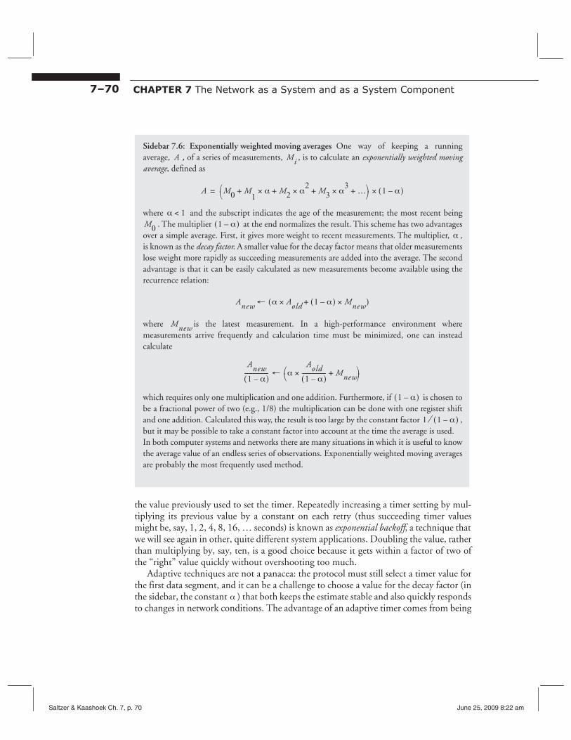
7–70 CHAPTER 7 The Network as a System and as a System Component
Sidebar 7.6: Exponentially weighted moving averages One way of keeping a running average, , of a series of measurements, , is to calculate an exponentially weighted moving average, defined as
where and the subscript indicates the age of the measurement; the most recent being . The multiplier at the end normalizes the result. This scheme has two advantages
over a simple average. First, it gives more weight to recent measurements. The multiplier, , is known as the decay factor. A smaller value for the decay factor means that older measurements lose weight more rapidly as succeeding measurements are added into the average. The second advantage is that it can be easily calculated as new measurements become available using the recurrence relation:
where is the latest measurement. In a high-performance environment where measurements arrive frequently and calculation time must be minimized, one can instead calculate
which requires only one multiplication and one addition. Furthermore, if is chosen to be a fractional power of two (e.g., 1/8) the multiplication can be done with one register shift and one addition. Calculated this way, the result is too large by the constant factor , but it may be possible to take a constant factor into account at the time the average is used. In both computer systems and networks there are many situations in which it is useful to know the average value of an endless series of observations. Exponentially weighted moving averages are probably the most frequently used method.
A Mi
A M0 M+ 1
α× M2 α× 2
M3 α× 3
…+ + +⎝ ⎠ ⎛ ⎞ 1 α–( )×=
α 1< M0 1 α–( )
α
A new ← α Aold× 1 α–( ) M new ×+( )
M new
A new 1 α–( )
----------------- ← α Aold 1 α–( )
-----------------× M new +⎝ ⎠ ⎛ ⎞
1 α–( )
1 1 α–( )⁄
the value previously used to set the timer. Repeatedly increasing a timer setting by multiplying its previous value by a constant on each retry (thus succeeding timer values might be, say, 1, 2, 4, 8, 16, … seconds) is known as exponential backoff, a technique that we will see again in other, quite different system applications. Doubling the value, rather than multiplying by, say, ten, is a good choice because it gets within a factor of two of the “right” value quickly without overshooting too much.
Adaptive techniques are not a panacea: the protocol must still select a timer value for the first data segment, and it can be a challenge to choose a value for the decay factor (in the sidebar, the constant α ) that both keeps the estimate stable and also quickly responds to changes in network conditions. The advantage of an adaptive timer comes from being
Saltzer & Kaashoek Ch. 7, p. 70 June 25, 2009 8:22 am
7.5 The End-to-End Layer 7–71
able to amortize the cost of an uninformed choice on that first data segment over the ensuing several segments.
A different method for minimizing use of fixed timers is for the receiving side of a stream of data segments to infer from the arrival of later data segments the loss of earlier ones and request their retransmission by sending a negative acknowledgment, or NAK. A NAK is simply a message that lists missing items. Since data segments may be delivered out of order, the recipient needs some way of knowing which segment is missing. For example, the sender might assign sequential numbers as nonces, so arrival of segments #13 and #14 without having previously received segment #12 might cause the recipient to send a NAK requesting retransmission of segment #12. To distinguish transmission delays from lost segments, the recipient must decide how long to wait before sending a NAK, but that decision can be made by counting later-arriving segments rather than by measuring a time interval.
Since the recipient reports lost packets, the sender does not need to be persistent, so it does not need to use a timer at all—that is, until it sends the last segment of a stream. Because the recipient can’t depend on later segment arrivals to discover that the last segment has been lost, that discovery still requires the help of a timer. With NAKs, the persistent-sender strategy with a timer is needed only once per stream, so the penalty for choosing a timer setting that is too long (or too short) is just one excessive delay (or one risk of an unnecessary duplicate transmission) on the last segment of the stream. Compared with using an adaptive timer on every segment of the stream, this is probably an improvement.
The appropriate conclusion about timers is that fixed timers are a terrible mechanism to include in an end-to-end protocol (or indeed anywhere—this conclusion applies to many applications of timers in systems). Adaptive timers work better, but add complexity and require careful thought to make them stable. Avoidance and minimization of timers are the better strategies, but it is usually impossible to completely eliminate them. Where timers must be used they should be designed with care and the designer should clearly document them as potential trouble spots.
7.5.3 Assurance of At-Most-Once Delivery: Duplicate Suppression
At-least-once delivery assurance was accomplished by remembering state at the sending side of the transport protocol: a copy of the data segment, its nonce, and a flag indicating that an acknowledgment is still needed. But a side effect of at-least-once delivery is that it tends to generate duplicates. To ensure at-most-once delivery, it is necessary to suppress these duplicates, as well as any other duplicates created elsewhere within the network, perhaps by a persistent sender in some link-layer protocol.
The mechanism of suppressing duplicates is a mirror image of the mechanism of at-least-once delivery: add state at the receiving side. We saw a preview of this mechanism in Section 7.1 of this chapter—the receiving side maintains a table of previously-seen nonces. Whenever a data segment arrives, the transport layer implementation checks the nonce of the incoming segment against the list of previously-seen nonces. If this nonce
Saltzer & Kaashoek Ch. 7, p. 71 June 25, 2009 8:22 am

7–72 CHAPTER 7 The Network as a System and as a System Component
is new, it adds the nonce to the list, delivers the data segment to the application, and sends an acknowledgment back to the sender. If the nonce is already in its list, it discards the data segment, but it resends the acknowledgment, in case the sender did not receive the previous one. If, in addition, the application has already sent a response to the original request, the transport protocol also resends that response.
The main problem with this technique is that the list of nonces maintained at the receiving side of the transport protocol may grow indefinitely, taking up space and, whenever a data segment arrives, taking time to search. Because they may have to be kept indefinitely, these nonces are described colorfully as tombstones. A challenge in designing a duplicate-suppression technique is to avoid accumulating an unlimited number of tombstones.
One possibility is for the sending side to use monotonically increasing sequence numbers for nonces, and include as an additional field in the end-to-end header of every data segment the highest sequence number for which it has received an acknowledgment. The receiving side can then discard that nonce and any others from that sender that are smaller, but it must continue to hold a nonce for the most recently-received data segment. This technique reduces the magnitude of the problem, but it leaves a dawning realization that it may never be possible to discard the last nonce, which threatens to become a genuine tombstone, one per sender. Two pragmatic responses to the tombstone problem are:
1. Move the problem somewhere else. For example, change the port number on which the protocol accepts new requests. The protocol should never reuse the old port number (the old port number becomes the tombstone), but if the port number space is large then it doesn’t matter.
2. Accept the possibility of making a mistake, but make its probability vanishingly small. If the sending side of the transport protocol always gives up and stops resending requests after, say, five retries, then the receiving side can safely discard nonces that are older than five network round-trip times plus some allowance for unusually large delays. This approach requires keeping track of the age of each nonce in the table, and it has some chance of failing if a packet that the network delayed a long time finally shows up. A simple defense against this form of failure is to wait a long time before discarding a tombstone.
Another form of the same problem concerns what to do when the computer at the receiving side crashes and restarts, losing its volatile memory. If the receiving side stores the list of previously handled nonces in volatile memory, following a crash it will not be able to recognize duplicates of packets that it handled before the crash. But if it stores that list in a non-volatile storage device such as a hard disk, it will have to do one write to that storage device for every message received. Writes to non-volatile media tend to be slow, so this approach may introduce a significant performance loss. To solve the problem without giving up performance, techniques parallel to the last two above are typically employed. For example, one can use a new port number each time the system restarts.
Saltzer & Kaashoek Ch. 7, p. 72 June 25, 2009 8:22 am
7.5 The End-to-End Layer 7–73
This technique requires remembering which port number was last used, but that number can be stored on a disk without hurting performance because it changes only once per restart. Or, if we know that the sending side of the transport protocol always gives up after some number of retries, whenever the receiving side restarts, it can simply ignore all packets until that number of round-trip times has passed since restarting. Either procedure may force the sending side to report delivery failure to its application, but that may be better than taking the risk of accepting duplicate data.
When techniques for at-least-once delivery (the persistent sender) and at-most-once delivery (duplicate detection) are combined, they produce an assurance that is called exactly-once delivery. This assurance is the one that would probably be wanted in an implementation of the Remote Procedure Call protocol of Chapter 4. Despite its name, and even if the sender is prepared to be infinitely persistent, exactly-once delivery is not a guarantee that the message will eventually be delivered. Instead, it ensures that if the message is delivered, it will be delivered only once, and if delivery fails, the sender will learn, by lack of acknowledgment despite repeated requests, that delivery probably failed. However, even if no acknowledgment returns, there is a still a possibility that the message was delivered. Section 9.6.2[on-line] introduces a protocol known as two-phase commit that can reduce the uncertainty by adding a persistent sender of the acknowledgement. Unfortunately, there is no way to completely eliminate the uncertainty.
7.5.4 Division into Segments and Reassembly of Long Messages
Recall that the requirements of the application determine the length of a message, but the network sets a maximum transmission unit, arising from limits on the length of a frame at the link layer. One of the jobs of the end-to-end transport protocol is to bridge this difference. Division of messages that are too long to fit in a single packet is relatively straightforward. Each resulting data segment must contain, in its end-to-end header, an identifier to show to which message this segment belongs and a segment number indicating where in the message the segment fits (e.g., “message 914, segment 3 of 7”). The message identifier and segment number together can also serve as the nonce used to ensure at-least-once and at-most-once delivery.
Reassembly is slightly more complicated because segments of the same message may arrive at the receiving side in any order, and may be mingled with segments from other messages. The reassembly process typically consists of allocating a buffer large enough to hold the entire message, placing the segments in the proper position within that buffer as they arrive, and keeping a checklist of which segments have not yet arrived. Once the message has been completely reassembled, the receiving side of the transport protocol can deliver the message to the application and discard the checklist.
Message division and reassembly is a special case of stream division and reassembly, the topic of Section 7.5.7, below.
7.5.5 Assurance of Data Integrity
Data integrity is the assurance that when a message is delivered, its contents are the same as when they left the sender. Adding data integrity to a protocol with a persistent sender
Saltzer & Kaashoek Ch. 7, p. 73 June 25, 2009 8:22 am
7–74 CHAPTER 7 The Network as a System and as a System Component
creates a reliable delivery protocol. Two additions are required, one at the sending side and one at the receiving side. The sending side of the protocol adds a field to the end-toend header or trailer containing a checksum of the contents of the application message. The receiving side recalculates the checksum from the received version of the reassembled message and compares it with the checksum that came with the message. Only if the two checksums match does the transport protocol deliver the reassembled message to the application and send an acknowledgment. If the checksums do not match the receiver discards the message and waits for the sending side to resend it. (One might suggest immediately sending a NAK, to alert the sending side to resend the data identified with that nonce, rather than waiting for timers to expire. This idea has the hazard that the source address that accompanies the data may have been corrupted along with the data. For this reason, sending a NAK on a checksum error isn’t usually done in end-toend protocols. However, as was described in Section 7.3.3, requesting retransmission as soon as an error is detected is useful at the link layer, where the other end of a point-topoint link is the only possible source.)
It might seem redundant for the transport protocol to provide a checksum, given that link layer protocols often also provide checksums. The reason the transport protocol might do so is an end-to-end argument: the link layer checksums protect the data only while it is in transit on the link. During the time the data is in the memory of a forwarding node, while being divided into multiple segments, being reassembled at the receiving end, or while being copied to the destination application buffer, it is still vulnerable to undetected accidents. An end-to-end transport checksum can help defend against those threats. On the other hand, reapplying the end-to-end argument suggests that an even better place for this checksum would be in the application program. But in the real world, many applications assume that a transport-protocol checksum covers enough of the threats to integrity that they don’t bother to apply their own checksum. Transport protocol checksums cater to this assumption.
As with all checksums, the assurance is not absolute. Its quality depends on the number of bits in the checksum, the structure of the checksum algorithm, and the nature of the likely errors. In addition, there remains a threat that someone has maliciously modified both the data and its checksum to match while enroute; this threat is explored briefly in Section 7.5.9, below, and in more depth in Chapter 11[on-line].
A related integrity concern is that a packet might be misdelivered, perhaps because its address field has been corrupted. Worse, the unintended recipient may even acknowledge receipt of the segment in the packet, leading the sender to believe that it was correctly delivered. The transport protocol can guard against this possibility by, on the sending side, including a copy of the destination address in the end-to-end segment header, and, on the receiving side, verifying that the address is the recipient’s own before delivering the packet to the application and sending an acknowledgment back.
Saltzer & Kaashoek Ch. 7, p. 74 June 25, 2009 8:22 am

3
N
7.5 The End-to-End Layer 7–75
7.5.6 End-to-End Performance: Overlapping and Flow Control
End-to-end transport of a multisegment message raises some questions of strategy for the transport protocol, including an interesting trade-off between complexity and performance. The simplest method of sending a multisegment message is to send one segment, wait for the receiving side to acknowledge that segment, then send the second segment, and so on. This protocol, known as lock-step, is illustrated in Figure 7.39. An important virtue of the lock-step protocol is that it is easy to see how to apply each of the previous end-to-end assurance techniques to one segment at a time. The downside is that transmitting a message that occupies N segments will take N network round-trip times. If the network transit time is large, both ends may spend most of their time waiting.
7.5.6.1 Overlapping Transmissions To avoid the wait times, we can employ a pipelining technique related to the pipelining described in Section 6.1.5: As soon as the first segment has been sent, immediately send the second one, then the third one, and so on, without waiting for acknowledgments. This technique allows both close spacing of transmissions and overlapping of transmissions with their corresponding acknowledgments. If nothing goes wrong, the technique leads to a timing diagram such as that of Figure 7.40. When the pipeline is completely filled, there may be several segments “in the net” traveling in both directions down transmission lines or sitting in the buffers of intermediate packet forwarders.
receiversender send first segment
segment 1 time
accept segment 1
Acknowledgment 1
segment 2
Acknowledgment 2
receive ACK, send second segment
accept segment 2
receive ACK, send third segment
• • •(repeat N times)
Acknowledgment N accept segment N
Done.
FIGURE 7.39
Lock-step transmission of multiple segments.
Saltzer & Kaashoek Ch. 7, p. 75 June 25, 2009 8:22 am
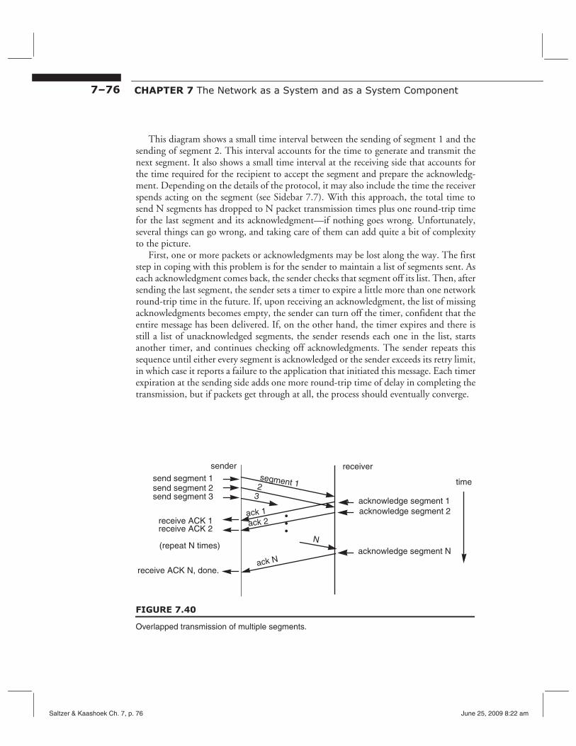
7–76 CHAPTER 7 The Network as a System and as a System Component
This diagram shows a small time interval between the sending of segment 1 and the sending of segment 2. This interval accounts for the time to generate and transmit the next segment. It also shows a small time interval at the receiving side that accounts for the time required for the recipient to accept the segment and prepare the acknowledgment. Depending on the details of the protocol, it may also include the time the receiver spends acting on the segment (see Sidebar 7.7). With this approach, the total time to send N segments has dropped to N packet transmission times plus one round-trip time for the last segment and its acknowledgment—if nothing goes wrong. Unfortunately, several things can go wrong, and taking care of them can add quite a bit of complexity to the picture.
First, one or more packets or acknowledgments may be lost along the way. The first step in coping with this problem is for the sender to maintain a list of segments sent. As each acknowledgment comes back, the sender checks that segment off its list. Then, after sending the last segment, the sender sets a timer to expire a little more than one network round-trip time in the future. If, upon receiving an acknowledgment, the list of missing acknowledgments becomes empty, the sender can turn off the timer, confident that the entire message has been delivered. If, on the other hand, the timer expires and there is still a list of unacknowledged segments, the sender resends each one in the list, starts another timer, and continues checking off acknowledgments. The sender repeats this sequence until either every segment is acknowledged or the sender exceeds its retry limit, in which case it reports a failure to the application that initiated this message. Each timer expiration at the sending side adds one more round-trip time of delay in completing the transmission, but if packets get through at all, the process should eventually converge.
sender segment 1
ack 1
2
ack N
ack 2
3
• •
N
receiver send segment 1 time send segment 2 send segment 3 acknowledge segment 1
acknowledge segment 2 receive ACK 1 receive ACK 2 •
(repeat N times) acknowledge segment N
receive ACK N, done.
FIGURE 7.40
Overlapped transmission of multiple segments.
Saltzer & Kaashoek Ch. 7, p. 76 June 25, 2009 8:22 am
7.5 The End-to-End Layer 7–77
Sidebar 7.7: What does an acknowledgment really mean? An end-to-end acknowledgment is a widely used technique for the receiving side to tell the sending side something of importance, but since there are usually several different things going on in the end-to-end layer, there can also be several different purposes for acknowledgments. Some possibilities include
• it is OK to stop the timer associated with the acknowledged data segment • it is OK to release the buffer holding a copy of the acknowledged segment • it is OK to send another segment • the acknowledged segment has been accepted for consideration • the work requested in the acknowledged segment has been completed.
In some protocols, a single acknowledgment serves several of those purposes, while in other protocols a different form of acknowledgment may be used for each one; there are endless combinations. As a result, whenever the word acknowledgment is used in the discussion of a protocol, it is a good idea to establish exactly what the acknowledgment really means. This understanding is especially important if one is trying to estimate round-trip times by measuring the time for an acknowledgment to return; in some protocols such a measurement would include time spent doing processing in the receiving application, while in other cases it would not.
If there really are five different kinds of acknowledgments, there is a concern that for every outgoing packet there might be five different packets returning with acknowledgments. In practice this is rarely the case because acknowledgments can be implemented as data items in the end-to-end header of any packet that happens to be going in the reverse direction. A single packet may thus carry any number of different kinds of acknowledgments and acknowledgments for a range of received packets, in addition to application data that may be flowing in the reverse direction. The technique of placing one or more acknowledgments in the header of the next packet that happens to be going in the reverse direction is known as piggybacking.
7.5.6.2 Bottlenecks, Flow Control, and Fixed Windows A second set of issues has to do with the relative speeds of the sender in generating segments, the entry point to the network in accepting them, any bottleneck inside the network in transmitting them, and the receiver in consuming them. The timing diagram and analysis above assumed that the bottleneck was at the sending side, either in the rate at which the sender generates segments or the rate that at which the first network link can transmit them.
A more interesting case is when the sender generates data, and the network transmits it, faster than the receiver can accept it, perhaps because the receiver has a slow processor and eventually runs out of buffer space to hold not-yet-processed data. When this is a possibility, the transport protocol needs to include some method of controlling the rate at which the sender generates data. This mechanism is called flow control. The basic con-
Saltzer & Kaashoek Ch. 7, p. 77 June 25, 2009 8:22 am

7–78 CHAPTER 7 The Network as a System and as a System Component
cept involved is that the sender starts by asking the receiver how much data the receiver can handle. The response from the receiver, which may be measured in bits, bytes, or segments, is known as a window. The sender asks permission to send, and the receiver responds by quoting a window size, as illustrated in Figure 7.41. The sender then sends that much data and waits until it receives permission to send more. Any intermediate acknowledgments from the receiver allow the sender to stop the associated timer and release the send buffer, but they cannot be used as permission to send more data because the receiver is only acknowledging data arrival, not data consumption. Once the receiver has actually consumed the data in its buffers, it sends permission for another window’s worth of data. One complication is that the implementation must guard against both missing permission messages that could leave the sender with a zero-sized window and also duplicated permission messages that could increase the window size more than the receiver intends: messages carrying window-granting permission require exactly-once delivery.
The window provided by the scheme of Figure 7.41 is called a fixed window. The lock-step protocol described earlier is a flow control scheme with a window that is one data segment in size. With any window scheme, one network round-trip time elapses between the receiver’s sending of a window-opening message and the arrival of the first data that takes advantage of the new window. Unless we are careful, this time will be pure delay experienced by both parties. A clever receiver could anticipate this delay, and send
receive permission,send segment 1 send segment 2 send segment 3 send segment 4
receive ACK 1 receive ACK 2 receive ACK 3 receive ACK 4,
wait …
receive permission,send segment 5 send segment 6
sender receiver
segment #1#2
ack # 2
#3
may I send?
yes, 4 segments
send 4 more
segment #5#6
• • •
ack # 1
ack # 3
ack # 4
#4
time receive request,open a 4-segmentwindow
buffer segment 1 buffer segment 2 buffer segment 3 buffer segment 4
finished processingsegments 1–4, reopenthe window
buffer segment 5 buffer segment 6
FIGURE 7.41
Flow control with a fixed window.
Saltzer & Kaashoek Ch. 7, p. 78 June 25, 2009 8:22 am
7.5 The End-to-End Layer 7–79
the window-opening message one round-trip time before it expects to be ready for more data. This form of prediction is still using a fixed window, but it keeps data flowing more smoothly. Unfortunately, it requires knowing the network round-trip time which, as the discussion of timers explained, is a hard thing to estimate. Exercises 7.13, on page 7–114, and 7.16, on page 7–115, explore the bang-bang protocol and pacing, two more variants on the fixed window idea.
7.5.6.3 Sliding Windows and Self-Pacing An even more clever scheme is the following: as soon as it has freed up a segment buffer, the receiver could immediately send permission for a window that is one segment larger (either by sending a separate message or, if there happens to be an ACK ready to go, piggy-backing on that ACK). The sender keeps track of how much window space is left, and increases that number whenever additional permission arrives. When a window can have space added to it on the fly it is called a sliding window. The advantage of a sliding window is that it can automatically keep the pipeline filled, without need to guess when it is safe to send permission-granting messages.
The sliding window appears to eliminate the need to know the network round-trip time, but this appearance is an illusion. The real challenge in flow control design is to develop a single flow control algorithm that works well under all conditions, whether the bottleneck is the sender’s rate of generating data, the network transmission capacity, or the rate at which the receiver can accept data. When the receiver is the bottleneck, the goal is to ensure that the receiver never waits. Similarly, when the sender is the bottleneck, the goal is to ensure that the sender never waits. When the network is the bottleneck, the goal is to keep the network moving data at its maximum rate. The question is what window size will achieve these goals.
The answer, no matter where the bottleneck is located, is determined by the bottleneck data rate and the round-trip time of the network. If we multiply these two quantities, the product tells us the amount of buffering, and thus the minimum window size, needed to ensure a continuous flow of data. That is,
window size ≥ round-trip time × bottleneck data rate
To see why, imagine for a moment that we are operating with a sliding window one segment in size. As we saw before, this window size creates a lock-step protocol with one segment delivered each round-trip time, so the realized data rate will be the window size divided by the round-trip time. Now imagine operating with a window of two segments. The network will then deliver two segments each round-trip time. The realized data rate is still the window size divided by the round-trip time, but the window size is twice as large. Now, continue to try larger window sizes until the realized data rate just equals the bottleneck data rate. At that point the window size divided by the round-trip time still tells us the realized data rate, so we have equality in the formula above. Any window size less than this will produce a realized data rate less than the bottleneck. The window size can be larger than this minimum, but since the realized data rate cannot exceed the bot-
Saltzer & Kaashoek Ch. 7, p. 79 June 25, 2009 8:22 am
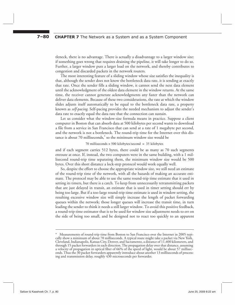
7–80 CHAPTER 7 The Network as a System and as a System Component
tleneck, there is no advantage. There is actually a disadvantage to a larger window size: if something goes wrong that requires draining the pipeline, it will take longer to do so. Further, a larger window puts a larger load on the network, and thereby contributes to congestion and discarded packets in the network routers.
The most interesting feature of a sliding window whose size satisfies the inequality is that, although the sender does not know the bottleneck data rate, it is sending at exactly that rate. Once the sender fills a sliding window, it cannot send the next data element until the acknowledgment of the oldest data element in the window returns. At the same time, the receiver cannot generate acknowledgments any faster than the network can deliver data elements. Because of these two considerations, the rate at which the window slides adjusts itself automatically to be equal to the bottleneck data rate, a property known as self-pacing. Self-pacing provides the needed mechanism to adjust the sender’s data rate to exactly equal the data rate that the connection can sustain.
Let us consider what the window-size formula means in practice. Suppose a client computer in Boston that can absorb data at 500 kilobytes per second wants to download a file from a service in San Francisco that can send at a rate of 1 megabyte per second, and the network is not a bottleneck. The round-trip time for the Internet over this distance is about 70 milliseconds,* so the minimum window size would be
70 milliseconds × 500 kilobytes/second = 35 kilobytes
and if each segment carries 512 bytes, there could be as many as 70 such segments enroute at once. If, instead, the two computers were in the same building, with a 1 millisecond round-trip time separating them, the minimum window size would be 500 bytes. Over this short distance a lock-step protocol would work equally well.
So, despite the effort to choose the appropriate window size, we still need an estimate of the round-trip time of the network, with all the hazards of making an accurate estimate. The protocol may be able to use the same round-trip time estimate that it used in setting its timers, but there is a catch. To keep from unnecessarily retransmitting packets that are just delayed in transit, an estimate that is used in timer setting should err by being too large. But if a too-large round-trip time estimate is used in window setting, the resulting excessive window size will simply increase the length of packet forwarding queues within the network; those longer queues will increase the transit time, in turn leading the sender to think it needs a still larger window. To avoid this positive feedback, a round-trip time estimator that is to be used for window size adjustment needs to err on the side of being too small, and be designed not to react too quickly to an apparent
* Measurements of round-trip time from Boston to San Francisco over the Internet in 2005 typically show a minimum of about 70 milliseconds. A typical route might take a packet via New York, Cleveland, Indianapolis, Kansas City, Denver, and Sacramento, a distance of 11,400 kilometers, and through 15 packet forwarders in each direction. The propagation delay over that distance, assuming a velocity of propagation in optical fiber of 66% of the speed of light, would be about 57 milliseconds. Thus the 30 packet forwarders apparently introduce about another 13 milliseconds of processing and transmission delay, roughly 430 microseconds per forwarder.
Saltzer & Kaashoek Ch. 7, p. 80 June 25, 2009 8:22 am
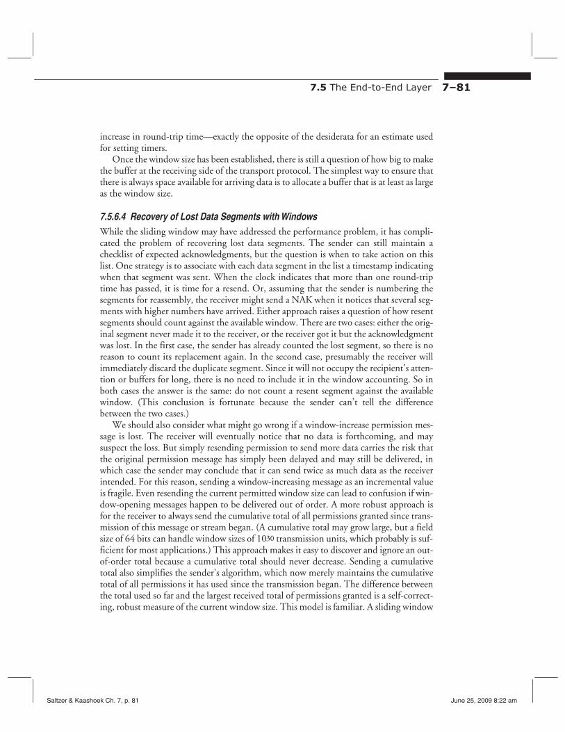
7.5 The End-to-End Layer 7–81
increase in round-trip time—exactly the opposite of the desiderata for an estimate used for setting timers.
Once the window size has been established, there is still a question of how big to make the buffer at the receiving side of the transport protocol. The simplest way to ensure that there is always space available for arriving data is to allocate a buffer that is at least as large as the window size.
7.5.6.4 Recovery of Lost Data Segments with Windows While the sliding window may have addressed the performance problem, it has complicated the problem of recovering lost data segments. The sender can still maintain a checklist of expected acknowledgments, but the question is when to take action on this list. One strategy is to associate with each data segment in the list a timestamp indicating when that segment was sent. When the clock indicates that more than one round-trip time has passed, it is time for a resend. Or, assuming that the sender is numbering the segments for reassembly, the receiver might send a NAK when it notices that several segments with higher numbers have arrived. Either approach raises a question of how resent segments should count against the available window. There are two cases: either the original segment never made it to the receiver, or the receiver got it but the acknowledgment was lost. In the first case, the sender has already counted the lost segment, so there is no reason to count its replacement again. In the second case, presumably the receiver will immediately discard the duplicate segment. Since it will not occupy the recipient’s attention or buffers for long, there is no need to include it in the window accounting. So in both cases the answer is the same: do not count a resent segment against the available window. (This conclusion is fortunate because the sender can’t tell the difference between the two cases.)
We should also consider what might go wrong if a window-increase permission message is lost. The receiver will eventually notice that no data is forthcoming, and may suspect the loss. But simply resending permission to send more data carries the risk that the original permission message has simply been delayed and may still be delivered, in which case the sender may conclude that it can send twice as much data as the receiver intended. For this reason, sending a window-increasing message as an incremental value is fragile. Even resending the current permitted window size can lead to confusion if window-opening messages happen to be delivered out of order. A more robust approach is for the receiver to always send the cumulative total of all permissions granted since transmission of this message or stream began. (A cumulative total may grow large, but a field size of 64 bits can handle window sizes of 1030 transmission units, which probably is sufficient for most applications.) This approach makes it easy to discover and ignore an out-of-order total because a cumulative total should never decrease. Sending a cumulative total also simplifies the sender’s algorithm, which now merely maintains the cumulative total of all permissions it has used since the transmission began. The difference between the total used so far and the largest received total of permissions granted is a self-correcting, robust measure of the current window size. This model is familiar. A sliding window
Saltzer & Kaashoek Ch. 7, p. 81 June 25, 2009 8:22 am
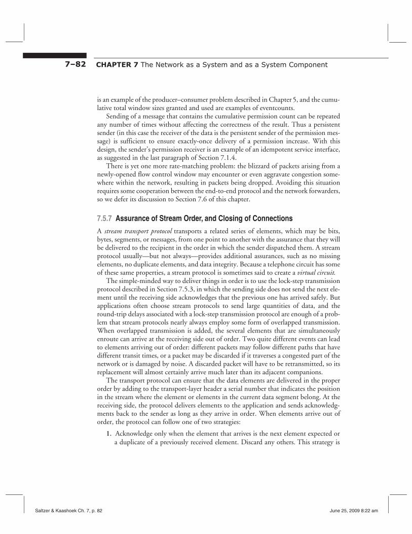
7–82 CHAPTER 7 The Network as a System and as a System Component
is an example of the producer–consumer problem described in Chapter 5, and the cumulative total window sizes granted and used are examples of eventcounts.
Sending of a message that contains the cumulative permission count can be repeated any number of times without affecting the correctness of the result. Thus a persistent sender (in this case the receiver of the data is the persistent sender of the permission message) is sufficient to ensure exactly-once delivery of a permission increase. With this design, the sender’s permission receiver is an example of an idempotent service interface, as suggested in the last paragraph of Section 7.1.4.
There is yet one more rate-matching problem: the blizzard of packets arising from a newly-opened flow control window may encounter or even aggravate congestion somewhere within the network, resulting in packets being dropped. Avoiding this situation requires some cooperation between the end-to-end protocol and the network forwarders, so we defer its discussion to Section 7.6 of this chapter.
7.5.7 Assurance of Stream Order, and Closing of Connections
A stream transport protocol transports a related series of elements, which may be bits, bytes, segments, or messages, from one point to another with the assurance that they will be delivered to the recipient in the order in which the sender dispatched them. A stream protocol usually—but not always—provides additional assurances, such as no missing elements, no duplicate elements, and data integrity. Because a telephone circuit has some of these same properties, a stream protocol is sometimes said to create a virtual circuit.
The simple-minded way to deliver things in order is to use the lock-step transmission protocol described in Section 7.5.3, in which the sending side does not send the next element until the receiving side acknowledges that the previous one has arrived safely. But applications often choose stream protocols to send large quantities of data, and the round-trip delays associated with a lock-step transmission protocol are enough of a problem that stream protocols nearly always employ some form of overlapped transmission. When overlapped transmission is added, the several elements that are simultaneously enroute can arrive at the receiving side out of order. Two quite different events can lead to elements arriving out of order: different packets may follow different paths that have different transit times, or a packet may be discarded if it traverses a congested part of the network or is damaged by noise. A discarded packet will have to be retransmitted, so its replacement will almost certainly arrive much later than its adjacent companions.
The transport protocol can ensure that the data elements are delivered in the proper order by adding to the transport-layer header a serial number that indicates the position in the stream where the element or elements in the current data segment belong. At the receiving side, the protocol delivers elements to the application and sends acknowledgments back to the sender as long as they arrive in order. When elements arrive out of order, the protocol can follow one of two strategies:
1. Acknowledge only when the element that arrives is the next element expected or a duplicate of a previously received element. Discard any others. This strategy is
Saltzer & Kaashoek Ch. 7, p. 82 June 25, 2009 8:22 am
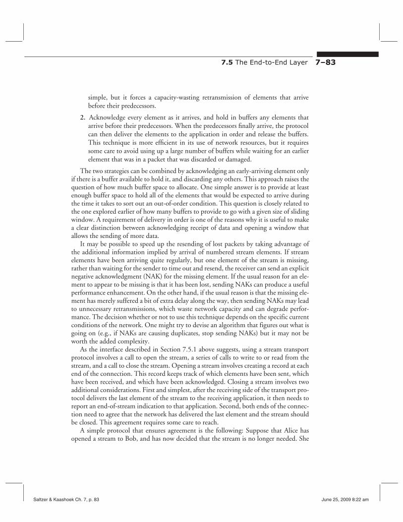
7.5 The End-to-End Layer 7–83
simple, but it forces a capacity-wasting retransmission of elements that arrive before their predecessors.
2. Acknowledge every element as it arrives, and hold in buffers any elements that arrive before their predecessors. When the predecessors finally arrive, the protocol can then deliver the elements to the application in order and release the buffers. This technique is more efficient in its use of network resources, but it requires some care to avoid using up a large number of buffers while waiting for an earlier element that was in a packet that was discarded or damaged.
The two strategies can be combined by acknowledging an early-arriving element only if there is a buffer available to hold it, and discarding any others. This approach raises the question of how much buffer space to allocate. One simple answer is to provide at least enough buffer space to hold all of the elements that would be expected to arrive during the time it takes to sort out an out-of-order condition. This question is closely related to the one explored earlier of how many buffers to provide to go with a given size of sliding window. A requirement of delivery in order is one of the reasons why it is useful to make a clear distinction between acknowledging receipt of data and opening a window that allows the sending of more data.
It may be possible to speed up the resending of lost packets by taking advantage of the additional information implied by arrival of numbered stream elements. If stream elements have been arriving quite regularly, but one element of the stream is missing, rather than waiting for the sender to time out and resend, the receiver can send an explicit negative acknowledgment (NAK) for the missing element. If the usual reason for an element to appear to be missing is that it has been lost, sending NAKs can produce a useful performance enhancement. On the other hand, if the usual reason is that the missing element has merely suffered a bit of extra delay along the way, then sending NAKs may lead to unnecessary retransmissions, which waste network capacity and can degrade performance. The decision whether or not to use this technique depends on the specific current conditions of the network. One might try to devise an algorithm that figures out what is going on (e.g., if NAKs are causing duplicates, stop sending NAKs) but it may not be worth the added complexity.
As the interface described in Section 7.5.1 above suggests, using a stream transport protocol involves a call to open the stream, a series of calls to write to or read from the stream, and a call to close the stream. Opening a stream involves creating a record at each end of the connection. This record keeps track of which elements have been sent, which have been received, and which have been acknowledged. Closing a stream involves two additional considerations. First and simplest, after the receiving side of the transport protocol delivers the last element of the stream to the receiving application, it then needs to report an end-of-stream indication to that application. Second, both ends of the connection need to agree that the network has delivered the last element and the stream should be closed. This agreement requires some care to reach.
A simple protocol that ensures agreement is the following: Suppose that Alice has opened a stream to Bob, and has now decided that the stream is no longer needed. She
Saltzer & Kaashoek Ch. 7, p. 83 June 25, 2009 8:22 am
7–84 CHAPTER 7 The Network as a System and as a System Component
begins persistently sending a close request to Bob, specifying the stream identifier. Bob, upon receiving a close request, checks to see if he agrees that the stream is no longer needed. If he does agree, he begins persistently sending a close acknowledgment, again specifying the stream identifier. Alice, upon receiving the close acknowledgment, can turn off her persistent sender and discard her record of the stream, confident that Bob has received all elements of the stream and will not be making any requests for retransmissions. In addition, she sends Bob a single “all done” message, containing the stream identifier. If she receives a duplicate of the close acknowledgment, her record of the stream will already be discarded, but it doesn’t matter; she can assume that this is a duplicate close acknowledgment from some previously closed stream and, from the information in the close acknowledgment, she can fabricate an “all done” message and send it to Bob. When Bob receives the “all done” message he can turn off his persistent sender and, confident that Alice agrees that there is no further use for the stream, discard his copy of the record of the stream. Alice and Bob can in the future safely discard any late duplicates that mention a stream for which they have no record. (The tombstone problem still exists for the stream itself. It would be a good idea for Bob to delay deletion of his record until there is no chance that a long-delayed duplicate of Alice’s original request to open the stream will arrive.)
7.5.8 Assurance of Jitter Control
Some applications, such as delivering sound or video to a person listening or watching on the spot, are known as real-time. For real-time applications, reliability, in the sense of never delivering an incorrect bit of data, is often less important than timely delivery. High reliability can actually be counter-productive if the transport protocol achieves it by requesting retransmission of a damaged data element, and then holds up delivery of the remainder of the stream until the corrected data arrives. What the application wants is continuous delivery of data, even if the data is not completely perfect. For example, if a few bits are wrong in one frame of a movie (note that this video use of the term “frame” has a meaning similar but not identical to the “frame” used in data communications), it probably won’t be noticed. In fact, if one video frame is completely lost in transit, the application program can probably get away with repeating the previous video frame while waiting for the following one to be delivered. The most important assurance that an end-to-end stream protocol can provide to a real-time application is that delivery of successive data elements be on a regular schedule. For example, a standard North American television set consumes one video frame every 33.37 milliseconds and the next video frame must be presented on that schedule.
Transmission across a forwarding network can produce varying transit times from one data segment to the next. In real-time applications, this variability in delivery time is known as jitter, and the requirement is to control the amount of jitter. The basic strategy is for the receiving side of the transport protocol to delay all arriving segments to make it look as though they had encountered the worst allowable amount of delay. One can in principle estimate an appropriate amount of extra buffering for the delayed seg-
Saltzer & Kaashoek Ch. 7, p. 84 June 25, 2009 8:22 am

7.5 The End-to-End Layer 7–85
ments as follows (assume for the television example that there is one video frame in each segment):
1. Measure the distribution of segment delivery delays between sending and receiving points and plot that distribution in a chart showing delay time versus frequency of that delay.
2. Choose an acceptable frequency of delivery failure. For a television application one might decide that 1 out of 100 video frames won’t be missed.
3. From the distribution, determine a delay time large enough to ensure that 99 out of 100 segments will be delivered in less than that delay time. Call this delay Dlong.
4. From the distribution determine the shortest delay time that is observed in practice. Call this value Dshort.
5. Now, provide enough buffering to delay every arriving segment so that it appears to have arrived with delay Dlong. The largest number of segments that would need to be buffered is
–Dlong DshortNumber of segment buffers = --------------------------------------Dheadway
where Dheadway is the average time between arriving segments. With this much buffering, we would expect that about one out of every 100 segments will arrive too late; when that occurs, the transport protocol simply reports “missing data” to the application and discards that segment if it finally does arrive.
In practice, there is no easy way to measure one-way segment delivery delay, so a common strategy is simply to set the buffer size by trial and error.
Although the goal of this technique is to keep the rate of missing video frames below the level of human perceptibility, you can sometimes see the technique fail when watching a television program that has been transmitted by satellite or via the Internet. Occasionally there may be a freeze-frame that persists long enough that you can see it, but that doesn’t seem to be one that the director intended. This event probably indicates that the transmission path was disrupted for a longer time than the available buffers were prepared to handle.
7.5.9 Assurance of Authenticity and Privacy
Most of the assurance-providing techniques described above are intended to operate in a benign environment, in which the designer assumes that errors can occur but that the errors are not maliciously constructed to frustrate the intended assurances. In many real-world environments, the situation is worse than that: one must defend against the threat that someone hostile intercepts and maliciously modifies packets, or that some end-toend layer participants violate a protocol with malicious intent.
To counter these threats, the end-to-end layer can apply two kinds of key-based mathematical transformations to the data:
Saltzer & Kaashoek Ch. 7, p. 85 June 25, 2009 8:22 am
7–86 CHAPTER 7 The Network as a System and as a System Component
1. sign and verify, to establish the authenticity of the source and the integrity of the contents of a message, and
2. encrypt and decrypt, to maintain the privacy of the contents of a message.
These two techniques can, if applied properly, be effective, but they require great care in design and implementation. Without such care, they may not work, but because they were applied the user may believe that they do, and thus have a false sense of security. A false assurance can be worse than no assurance at all. The issues involved in providing security assurances are a whole subject in themselves, and they apply to many system components in addition to networks, so we defer them to Chapter 11[on-line], which provides an in-depth discussion of protecting information in computer systems.
With this examination of end-to-end topics, we have worked our way through the highest layer that we identify as part of the network. The next section of this chapter, on congestion control, is a step sideways, to explore a topic that requires cooperation of more than one layer.
7.6 A Network System Design Issue: Congestion Control
7.6.1 Managing Shared Resources
Chapters 5 and 6 discussed shared resources and their management: a thread manager creates many virtual processors from a few real, shared processors that must then be scheduled, and a multilevel memory manager creates the illusion of large, fast virtual memories for several clients by combining a small and fast shared memory with large and slow storage devices. In both cases we looked at relatively simple management mechanisms because more complex mechanisms aren’t usually needed. In the network context, the resource that is shared is a set of communication links and the supporting packet forwarders. The geographically and administratively distributed nature of those components and their users adds delay and complication to resource management, so we need to revisit the topic.
In Section 7.1.2 of this chapter we saw how queues manage the problem that packets may arrive at a packet switch at a time when the outgoing link is already busy transmitting another packet, and Figure 7.6 showed the way that queues grow with increased utilization of the link. This same phenomenon applies to processor scheduling and supermarket checkout lines: any time there is a shared resource, and the demand for that resource comes from several statistically independent sources, there will be fluctuations in the arrival of load, and thus in the length of the queue and the time spent waiting for service. Whenever the offered load (in the case of a packet switch, that is the rate at which packets arrive and need to be forwarded) is greater than the capacity (the rate at which the switch can forward packets) of a resource for some duration, the resource is overloaded for that time period.
Saltzer & Kaashoek Ch. 7, p. 86 June 25, 2009 8:22 am
7.6 A Network System Design Issue: Congestion Control 7–87
When sources are statistically independent of one another, occasional overload is inevitable but its significance depends critically on how long it lasts. If the duration is comparable to the service time, which is the typical time for the resource to handle one customer (in a supermarket), one thread (in a processor manager), or one packet (in a packet forwarder), then a queue is simply an orderly way to delay some requests for service until a later time when the offered load drops below the capacity of the resource. Put another way, a queue handles short bursts of too much demand by time-averaging with adjacent periods when there is excess capacity.
If, on the other hand, overload persists for a time significantly longer than the service time, there begins to develop a risk that the system will fail to meet some specification such as maximum delay or acceptable response time. When this occurs, the resource is said to be congested. Congestion is not a precisely defined concept. The duration of overload that is required to classify a resource as congested is a matter of judgement, and different systems (and observers) will use different thresholds.
Congestion may be temporary, in which case clever resource management schemes may be able to rescue the situation, or it may be chronic, meaning that the demand for service continually exceeds the capacity of the resource. If the congestion is chronic, the length of the queue will grow without bound until something breaks: the space allocated for the queue may be exceeded, the system may fail completely, or customers may go elsewhere in disgust.
The stability of the offered load is another factor in the frequency and duration of congestion. When the load on a resource is aggregated from a large number of statistically independent small sources, averaging can reduce the frequency and duration of load peaks. On the other hand, if the load comes from a small number of large sources, even if the sources are independent, the probability that they all demand service at about the same time can be high enough that congestion can be frequent or long-lasting.
A counter-intuitive concern of shared resource management is that competition for a resource sometimes leads to wasting of that resource. For example, in a grocery store, customers who are tired of waiting in the checkout line may just walk out of the store, leaving filled shopping carts behind. Someone has to put the goods from the abandoned carts back on the shelves. Suppose that one or two of the checkout clerks leave their registers to take care of the accumulating abandoned carts. The rate of sales being rung up drops while they are away from their registers, so the queues at the remaining registers grow longer, causing more people to abandon their carts, and more clerks will have to turn their attention to restocking. Eventually, the clerks will be doing nothing but restocking and the number of sales rung up will drop to zero. This regenerative overload phenomenon is called congestion collapse. Figure 7.42 plots the useful work getting done as the offered load increases, for three different cases of resource limitation and waste, including one that illustrates collapse. Congestion collapse is dangerous because it can be self-sustaining. Once temporary congestion induces a collapse, even if the offered load drops back to a level that the resource could handle, the already-induced waste rate can continue to exceed the capacity of the resource, causing it to continue to waste the resource and thus remain congested indefinitely.
Saltzer & Kaashoek Ch. 7, p. 87 June 25, 2009 8:22 am

7–88 CHAPTER 7 The Network as a System and as a System Component
When developing or evaluating a resource management scheme, it is important to keep in mind that you can’t squeeze blood out of a turnip: if a resource is congested, either temporarily or chronically, delays in receiving service are inevitable. The best a management scheme can do is redistribute the total amount of delay among waiting customers. The primary goal of resource management is usually quite simple: to avoid congestion collapse. Occasionally other goals, such as enforcing a policy about who gets delayed, are suggested, but these goals are often hard to define and harder to achieve. (Doling out delays is a tricky business; overall satisfaction may be higher if a resource serves a few customers well and completely discourages the remainder, rather than leaving all equally disappointed.)
Chapter 6 suggested two general approaches to managing congestion. Either:
• increase the capacity of the resource, or • reduce the offered load.
In both cases the goal is to move quickly to a state in which the load is less than the capacity of the resource. When measures are taken to reduce offered load, it is useful to separately identify the intended load, which would have been offered in the absence of
useful work
offered load
unlimited resource
limited resource with no waste
congestion collapse
capacity of a limited resource
done
FIGURE 7.42
Offered load versus useful work done. The more work offered to an ideal unlimited resource, the more work gets done, as indicated by the 45-degree unlimited resource line. Real resources are limited, but in the case with no waste, useful work asymptotically approaches the capacity of the resource. On the other hand, if overloading the resource also wastes it, useful work can decline when offered load increases, as shown by the congestion collapse line.
Saltzer & Kaashoek Ch. 7, p. 88 June 25, 2009 8:22 am
7.6 A Network System Design Issue: Congestion Control 7–89
control. Of course, in reducing offered load, the amount by which it is reduced doesn’t really go away, it is just deferred to a later time. Reducing offered load acts by averaging periods of overload with periods of excess capacity, just like queuing, but with involvement of the source of the load, and typically over a longer period of time.
To increase capacity or to reduce offered load it is necessary to provide feedback to one or more control points. A control point is an entity that determines, in the first case, the amount of resource that is available and, in the second, the load being offered. A congestion control system is thus a feedback system, and delay in the feedback path can lead to oscillations in load and in useful work done.
For example, in a supermarket, a common strategy is for the store manager to watch the queues at the checkout lines; whenever there are more than two or three customers in any line the manager calls for staff elsewhere in the store to drop what they are doing and temporarily take stations as checkout clerks, thereby increasing capacity. In contrast, when you call a customer support telephone line you may hear an automatic response message that says something such as, “Your call is important to us. It will be approximately 21 minutes till we are able to answer it.” That message will probably lead some callers to hang up and try again at a different time, thereby decreasing (actually deferring) the offered load. In both the supermarket and the telephone customer service system, it is easy to create oscillations. By the time the fourth supermarket clerk stops stacking dog biscuits and gets to the front of the store, the lines may have vanished, and if too many callers decide to hang up, the customer service representatives may find there is no one left to talk to.
In the commercial world, the choice between these strategies is a complex trade-off involving economics, physical limitations, reputation, and customer satisfaction. The same thing is true inside a computer system or network.
7.6.2 Resource Management in Networks
In a computer network, the shared resources are the communication links and the processing and buffering capacity of the packet forwarders. There are several things that make this resource management problem more difficult than, say, scheduling a processor among competing threads.
1. There is more than one resource. Even a small number of resources can be used up in an alarmingly large number of different ways, and the mechanisms needed to keep track of the situation can rapidly escalate in complexity. In addition, there can be dynamic interactions among different resources—as one nears capacity it may push back on another, which may push back on yet another, which may push back on the first one. These interactions can create either deadlock or livelock, depending on the details.
2. It is easy to induce congestion collapse. The usually beneficial independence of the layers of a packet forwarding network contributes to the ease of inducing congestion collapse. As queues for a particular communication link grow, delays
Saltzer & Kaashoek Ch. 7, p. 89 June 25, 2009 8:22 am
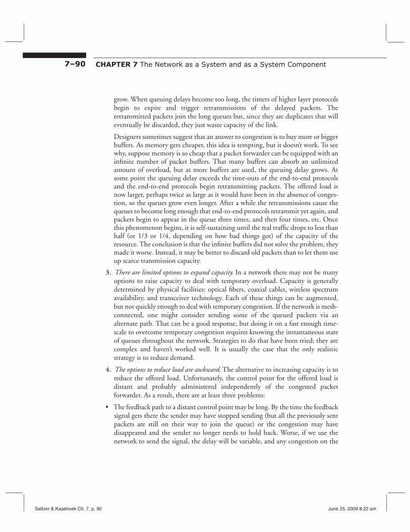
7–90 CHAPTER 7 The Network as a System and as a System Component
grow. When queuing delays become too long, the timers of higher layer protocols begin to expire and trigger retransmissions of the delayed packets. The retransmitted packets join the long queues but, since they are duplicates that will eventually be discarded, they just waste capacity of the link.
Designers sometimes suggest that an answer to congestion is to buy more or bigger buffers. As memory gets cheaper, this idea is tempting, but it doesn’t work. To see why, suppose memory is so cheap that a packet forwarder can be equipped with an infinite number of packet buffers. That many buffers can absorb an unlimited amount of overload, but as more buffers are used, the queuing delay grows. At some point the queuing delay exceeds the time-outs of the end-to-end protocols and the end-to-end protocols begin retransmitting packets. The offered load is now larger, perhaps twice as large as it would have been in the absence of congestion, so the queues grow even longer. After a while the retransmissions cause the queues to become long enough that end-to-end protocols retransmit yet again, and packets begin to appear in the queue three times, and then four times, etc. Once this phenomenon begins, it is self-sustaining until the real traffic drops to less than half (or 1/3 or 1/4, depending on how bad things got) of the capacity of the resource. The conclusion is that the infinite buffers did not solve the problem, they made it worse. Instead, it may be better to discard old packets than to let them use up scarce transmission capacity.
3. There are limited options to expand capacity. In a network there may not be many options to raise capacity to deal with temporary overload. Capacity is generally determined by physical facilities: optical fibers, coaxial cables, wireless spectrum availability, and transceiver technology. Each of these things can be augmented, but not quickly enough to deal with temporary congestion. If the network is mesh-connected, one might consider sending some of the queued packets via an alternate path. That can be a good response, but doing it on a fast enough time-scale to overcome temporary congestion requires knowing the instantaneous state of queues throughout the network. Strategies to do that have been tried; they are complex and haven’t worked well. It is usually the case that the only realistic strategy is to reduce demand.
4. The options to reduce load are awkward. The alternative to increasing capacity is to reduce the offered load. Unfortunately, the control point for the offered load is distant and probably administered independently of the congested packet forwarder. As a result, there are at least three problems:
• The feedback path to a distant control point may be long. By the time the feedback signal gets there the sender may have stopped sending (but all the previously sent packets are still on their way to join the queue) or the congestion may have disappeared and the sender no longer needs to hold back. Worse, if we use the network to send the signal, the delay will be variable, and any congestion on the
Saltzer & Kaashoek Ch. 7, p. 90 June 25, 2009 8:22 am

7.6 A Network System Design Issue: Congestion Control 7–91
path back may mean that the signal gets lost. The feedback system must be robust to deal with all these eventualities.
• The control point (in this case, an end-to-end protocol or application) must be capable of reducing its offered load. Some end-to-end protocols can do this quite easily, but others may not be able to. For example, a stream protocol that is being used to send files can probably reduce its average data rate on short notice. On the other hand, a real-time video transmission protocol may have a commitment to deliver a certain number of bits every second. A single-packet request/response protocol will have no control at all over the way it loads the network; control must be exerted by the application, which means there must be some way of asking the application to cooperate—if it can.
• The control point must be willing to cooperate. If the congestion is discovered by the network layer of a packet forwarder, but the control point is in the end-to-end layer of a leaf node, there is a good chance these two entities are under the responsibility of different administrations. In that case, obtaining cooperation can be problematic; the administration of the control point may be more interested in keeping its offered load equal to its intended load in the hope of capturing more of the capacity in the face of competition.
These problems make it hard to see how to apply a central planning approach such as the one that worked in the grocery store. Decentralized schemes seem more promising. Many mechanisms have been devised to try to manage network congestion. Sections 7.6.3 and 7.6.4 describe the design considerations surrounding one set of decentralized mechanisms, similar to the ones that are currently used in the public Internet. These mechanisms are not especially well understood, but they not only seem to work, they have allowed the Internet to operate over an astonishing range of capacity. In fact, the Internet is probably the best existing counterexample of the incommensurate scaling rule. Recall that the rule suggests that a system needs to be redesigned whenever any important parameter changes by a factor of ten. The Internet has increased in scale from a few hundred attachment points to a few hundred million attachment points with only modest adjustments to its underlying design.
7.6.3 Cross-layer Cooperation: Feedback
If the designer can arrange for cross-layer cooperation, then one way to attack congestion would be for the packet forwarder that notices congestion to provide feedback to one or more end-to-end layer sources, and for the end-to-end source to respond by reducing its offered load.
Several mechanisms have been suggested for providing feedback. One of the first ideas that was tried is for the congested packet forwarder to send a control message, called a source quench, to one or more of the source addresses that seems to be filling the queue. Unfortunately, preparing a control message distracts the packet forwarder at a time when
Saltzer & Kaashoek Ch. 7, p. 91 June 25, 2009 8:22 am
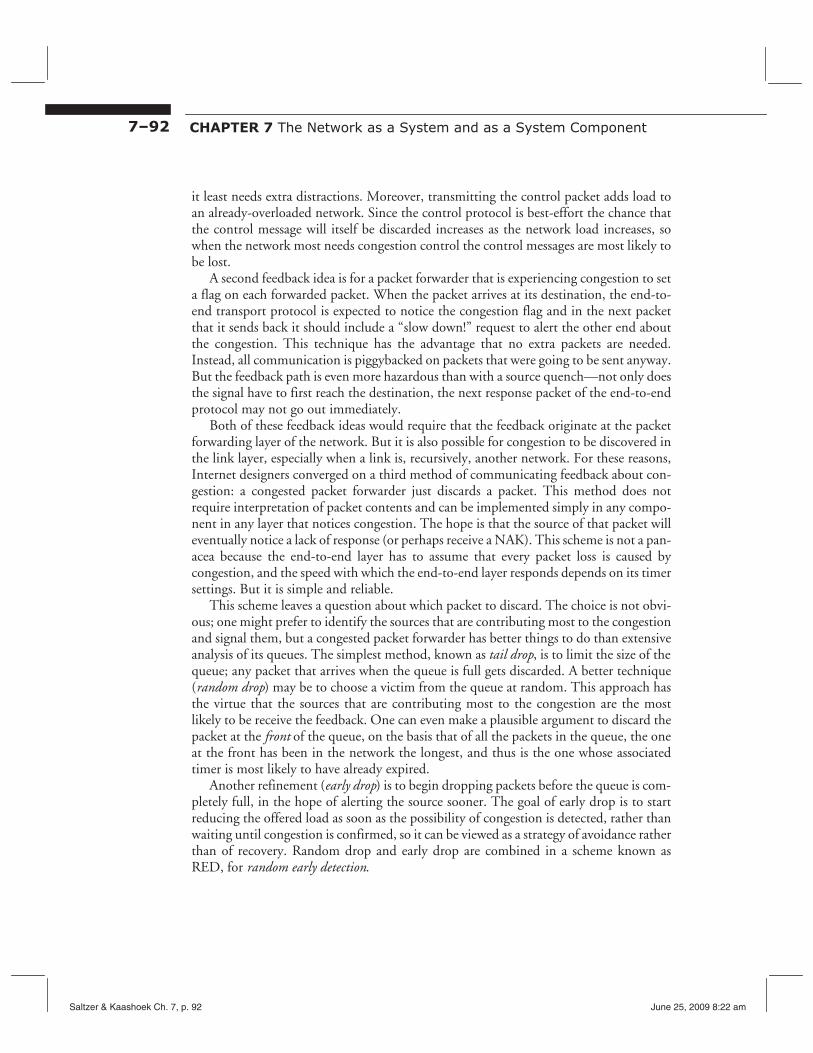
7–92 CHAPTER 7 The Network as a System and as a System Component
it least needs extra distractions. Moreover, transmitting the control packet adds load to an already-overloaded network. Since the control protocol is best-effort the chance that the control message will itself be discarded increases as the network load increases, so when the network most needs congestion control the control messages are most likely to be lost.
A second feedback idea is for a packet forwarder that is experiencing congestion to set a flag on each forwarded packet. When the packet arrives at its destination, the end-toend transport protocol is expected to notice the congestion flag and in the next packet that it sends back it should include a “slow down!” request to alert the other end about the congestion. This technique has the advantage that no extra packets are needed. Instead, all communication is piggybacked on packets that were going to be sent anyway. But the feedback path is even more hazardous than with a source quench—not only does the signal have to first reach the destination, the next response packet of the end-to-end protocol may not go out immediately.
Both of these feedback ideas would require that the feedback originate at the packet forwarding layer of the network. But it is also possible for congestion to be discovered in the link layer, especially when a link is, recursively, another network. For these reasons, Internet designers converged on a third method of communicating feedback about congestion: a congested packet forwarder just discards a packet. This method does not require interpretation of packet contents and can be implemented simply in any component in any layer that notices congestion. The hope is that the source of that packet will eventually notice a lack of response (or perhaps receive a NAK). This scheme is not a panacea because the end-to-end layer has to assume that every packet loss is caused by congestion, and the speed with which the end-to-end layer responds depends on its timer settings. But it is simple and reliable.
This scheme leaves a question about which packet to discard. The choice is not obvious; one might prefer to identify the sources that are contributing most to the congestion and signal them, but a congested packet forwarder has better things to do than extensive analysis of its queues. The simplest method, known as tail drop, is to limit the size of the queue; any packet that arrives when the queue is full gets discarded. A better technique (random drop) may be to choose a victim from the queue at random. This approach has the virtue that the sources that are contributing most to the congestion are the most likely to be receive the feedback. One can even make a plausible argument to discard the packet at the front of the queue, on the basis that of all the packets in the queue, the one at the front has been in the network the longest, and thus is the one whose associated timer is most likely to have already expired.
Another refinement (early drop) is to begin dropping packets before the queue is completely full, in the hope of alerting the source sooner. The goal of early drop is to start reducing the offered load as soon as the possibility of congestion is detected, rather than waiting until congestion is confirmed, so it can be viewed as a strategy of avoidance rather than of recovery. Random drop and early drop are combined in a scheme known as RED, for random early detection.
Saltzer & Kaashoek Ch. 7, p. 92 June 25, 2009 8:22 am

7.6 A Network System Design Issue: Congestion Control 7–93
7.6.4 Cross-layer Cooperation: Control
Suppose that the end-to-end protocol implementation learns of a lost packet. Sidebar 7.8: The tragedy of the commons
What then? One possibility is that it just “Picture a pasture open to all…As a rational
drives forward, retransmitting the lost being, each herdsman seeks to maximize his
packet and continuing to send more data gain…he asks, ‘What is the utility to me of
as rapidly as its application supplies it. The adding one more animal to my herd?’ This
end-to-end protocol implementation is in utility has one negative and one positive
control, and there is nothing compelling it component…Since the herdsman receives all
to cooperate. Indeed, it may discover that the proceeds from the sale of the additional animal, the positive utility is nearly +1.
by sending packets at the greatest rate it Since, however, the effects of overgrazing are
can sustain, it will push more data through shared by all the herdsmen, the negative the congested packet forwarder than it utility for any particular decision-makingwould otherwise. The problem, of course, herdsman is only a fraction of –1. is that if this is the standard mode of operation of every client, congestion will set in “Adding together the component partial
and all clients of the network will suffer, as utilities, the rational herdsman concludes
predicted by the tragedy of the commons that the only sensible course for him to
(see Sidebar 7.8). pursue is to add another animal to his herd.
There are at least two things that the And another…. But this is the conclusion
end-to-end protocol can do to cooperate. reached by each and every rational herdsman
The first is to be careful about its use of sharing a commons. Therein is the tragedy.
timers, and the second is to pace the rate at Each man is locked into a system that
which it sends data, a technique known as compels him to increase his herd without limit—in a world that is limited…Freedom automatic rate adaptation. Both these
things require having an estimate of the in a commons brings ruin to all.”
round-trip time between the two ends of — Garrett Hardin, Science 162, 3859
the protocol. [Suggestions for Further Reading 1.4.5]
The usual way of detecting a lost packet in a best-effort network is to set a timer to expire after a little more than one round-trip time, and assume that if an acknowledgment has not been received by then the packet is lost. In Section 7.5 of this chapter we introduced timers as a way of ensuring at-leastonce delivery via a best-effort network, expecting that lost packets had encountered mishaps such as misrouting, damage in transmission, or an overflowing packet buffer. With congestion management in operation, the dominant reason for timer expiration is probably that either a queue in the network has grown too long or a packet forwarder has intentionally discarded the packet. The designer needs to take this additional consideration into account when choosing a value for a retransmit timer.
As described in Section 7.5.6, a protocol can develop an estimate of the round trip time by directly measuring it for the first packet exchange and then continuing to update that estimate as additional packets flow back and forth. Then, if congestion develops, queuing delays will increase the observed round-trip times for individual packets, and
Saltzer & Kaashoek Ch. 7, p. 93 June 25, 2009 8:22 am
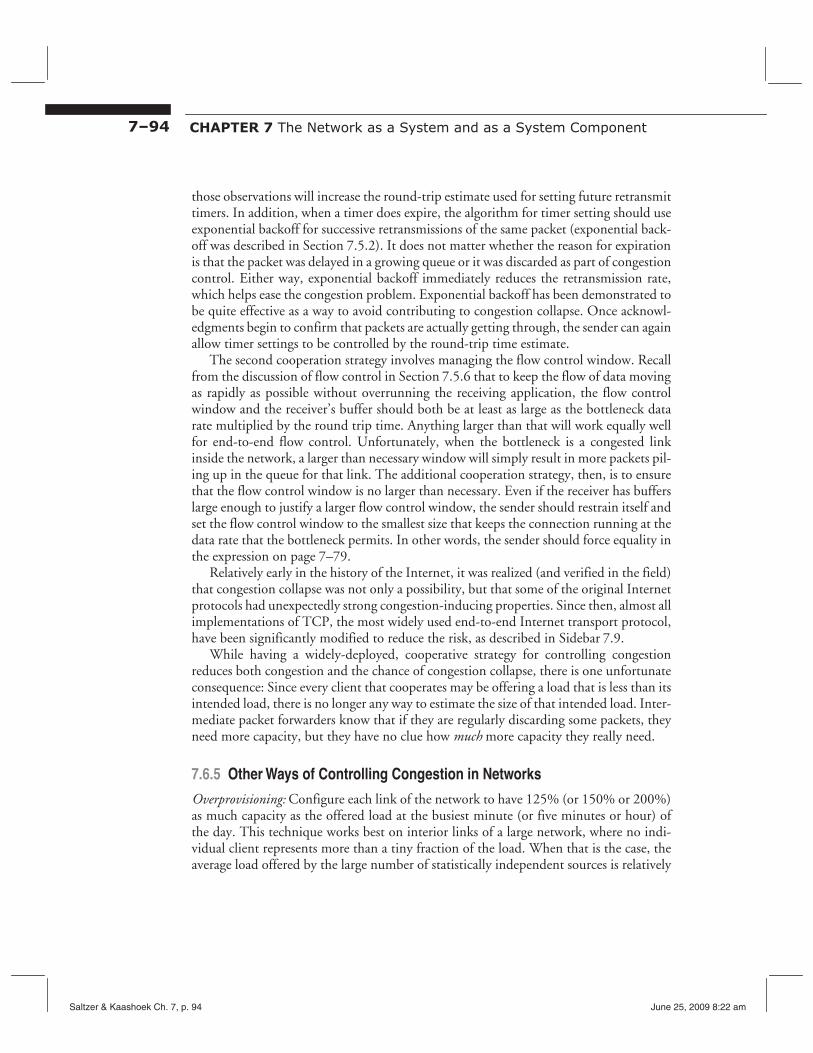
7–94 CHAPTER 7 The Network as a System and as a System Component
those observations will increase the round-trip estimate used for setting future retransmit timers. In addition, when a timer does expire, the algorithm for timer setting should use exponential backoff for successive retransmissions of the same packet (exponential back-off was described in Section 7.5.2). It does not matter whether the reason for expiration is that the packet was delayed in a growing queue or it was discarded as part of congestion control. Either way, exponential backoff immediately reduces the retransmission rate, which helps ease the congestion problem. Exponential backoff has been demonstrated to be quite effective as a way to avoid contributing to congestion collapse. Once acknowledgments begin to confirm that packets are actually getting through, the sender can again allow timer settings to be controlled by the round-trip time estimate.
The second cooperation strategy involves managing the flow control window. Recall from the discussion of flow control in Section 7.5.6 that to keep the flow of data moving as rapidly as possible without overrunning the receiving application, the flow control window and the receiver’s buffer should both be at least as large as the bottleneck data rate multiplied by the round trip time. Anything larger than that will work equally well for end-to-end flow control. Unfortunately, when the bottleneck is a congested link inside the network, a larger than necessary window will simply result in more packets piling up in the queue for that link. The additional cooperation strategy, then, is to ensure that the flow control window is no larger than necessary. Even if the receiver has buffers large enough to justify a larger flow control window, the sender should restrain itself and set the flow control window to the smallest size that keeps the connection running at the data rate that the bottleneck permits. In other words, the sender should force equality in the expression on page 7–79.
Relatively early in the history of the Internet, it was realized (and verified in the field) that congestion collapse was not only a possibility, but that some of the original Internet protocols had unexpectedly strong congestion-inducing properties. Since then, almost all implementations of TCP, the most widely used end-to-end Internet transport protocol, have been significantly modified to reduce the risk, as described in Sidebar 7.9.
While having a widely-deployed, cooperative strategy for controlling congestion reduces both congestion and the chance of congestion collapse, there is one unfortunate consequence: Since every client that cooperates may be offering a load that is less than its intended load, there is no longer any way to estimate the size of that intended load. Intermediate packet forwarders know that if they are regularly discarding some packets, they need more capacity, but they have no clue how much more capacity they really need.
7.6.5 Other Ways of Controlling Congestion in Networks
Overprovisioning: Configure each link of the network to have 125% (or 150% or 200%) as much capacity as the offered load at the busiest minute (or five minutes or hour) of the day. This technique works best on interior links of a large network, where no individual client represents more than a tiny fraction of the load. When that is the case, the average load offered by the large number of statistically independent sources is relatively
Saltzer & Kaashoek Ch. 7, p. 94 June 25, 2009 8:22 am

7.6 A Network System Design Issue: Congestion Control 7–95
Sidebar 7.9: Retrofitting TCP The Transmission Control Protocol (TCP), probably the most widely used end-to-end transport protocol of the Internet, was designed in 1974, At that time, previous experience was limited to lock-step protocols. on networks with no more than a few hundred nodes. As a result, avoiding congestion collapse was not in its list of requirements. About a decade later, when the Internet first began to expand rapidly, this omission was noticed, and a particular collapse-inducing feature of its design drew attention.
The only form of acknowledgment in the original TCP was “I have received all the bytes up to X”. There was no way for a receiver to say, for example, “I am missing bytes Y through Z”. In consequence when a timer expired because some packet or its acknowledgment was lost, as soon as the sender retransmitted that packet the timer of the next packet expired, causing its retransmission. This process would repeat until the next acknowledgment finally returned, a full round trip (and full flow control window) later. On long-haul routes, where flow control windows might be fairly large, if an overloaded packet forwarder responded to congestion by discarding a few packets (each perhaps from a different TCP connection), each discarded packet would trigger retransmission of a window full of packets, and the ensuing blizzard of retransmitted packets could immediately induce congestion collapse. In addition, an insufficiently adaptive time-out scheme ensured that the problem would occur frequently.
By the time this effect was recognized, TCP was widely deployed, so changes to the protocol were severely constrained. The designers found a way to change the implementation without changing the data formats. The goal was to allow new and old implementations to interoperate, so new implementations could gradually replace the old. The new implementation works by having the sender tinker with the size of the flow control window (Warning: this explanation is somewhat oversimplified!):
1. Slow start. When starting a new connection, send just one packet, and wait for its acknowledgment. Then, for each acknowledged packet, add one to the window size and send two packets. The result is that in each round trip time, the number of packets that the sender dispatches doubles. This doubling procedure continues until one of three things happens: (1) the sender reaches the window size suggested by the receiver, in which case the network is not the bottleneck, and the sender maintains the window at that size; (2) all the available data has been dispatched; or (3) the sender detects that a packet it sent has been discarded, as described in step 2.
2. Duplicate acknowledgment: The receiving TCP implementation is modified very slightly: whenever it receives an out-of-order packet, it sends back a duplicate of its latest acknowledgment. The idea is that a duplicate acknowledgment can be interpreted by the sender as a negative acknowledgment for the next unacknowledged packet.
3. Equilibrium: Upon duplicate acknowledgment, the sender retransmits just the first unacknowledged packet and also drops its window size to some fixed fraction (for example, 1/2) of its previous size. From then on it operates in an equilibrium mode in which it continues to watch for duplicate acknowledgments but it also probes gently to see if more capacity might be available. The equilibrium mode has two components:
(Sidebar continues)
Saltzer & Kaashoek Ch. 7, p. 95 June 25, 2009 8:22 am
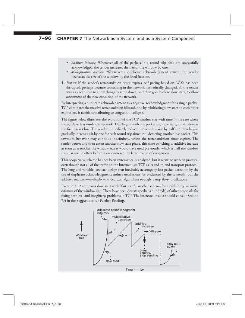
Saltzer & Kaashoek Ch. 7, p. 96 June 25, 2009 8:22 am
CHAPTER 7 The Network as a System and as a System Component 7–96
• Additive increase: Whenever all of the packets in a round trip time are successfully acknowledged, the sender increases the size of the window by one.
• Multiplicative decrease: Whenever a duplicate acknowledgment arrives, the sender decreases the size of the window by the fixed fraction.
4. Restart: If the sender’s retransmission timer expires, self-pacing based on ACKs has been disrupted, perhaps because something in the network has radically changed. So the sender waits a short time to allow things to settle down, and then goes back to slow start, to allow assessment of the new condition of the network.
By interpreting a duplicate acknowledgment as a negative acknowledgment for a single packet, TCP eliminates the massive retransmission blizzard, and by reinitiating slow start on each timer expiration, it avoids contributing to congestion collapse.
The figure below illustrates the evolution of the TCP window size with time in the case where the bottleneck is inside the network. TCP begins with one packet and slow start, until it detects the first packet loss. The sender immediately reduces the window size by half and then begins gradually increasing it by one for each round trip time until detecting another lost packet. This sawtooth behavior may continue indefinitely, unless the retransmission timer expires. The sender pauses and then enters another slow start phase, this time switching to additive increase as soon as it reaches the window size it would have used previously, which is half the window size that was in effect before it encountered the latest round of congestion.
This cooperative scheme has not been systematically analyzed, but it seems to work in practice, even though not all of the traffic on the Internet uses TCP as its end-to-end transport protocol. The long and variable feedback delays that inevitably accompany lost packet detection by the use of duplicate acknowledgments induce oscillations (as evidenced by the sawteeth) but the additive increase—multiplicative decrease algorithms strongly damp those oscillations.
Exercise 7.12 compares slow start with “fast start”, another scheme for establishing an initial estimate of the window size. There have been dozens (perhaps hundreds) of other proposals for fixing both real and imaginary, problems in TCP. The interested reader should consult Section 7.4 in the Suggestions for Further Reading.
Window size
slow start
multiplicativedecrease
additive increase
timer expires,
slow start,
delay
again
duplicate acknowledgment
stop sending
received
Time
7.6 A Network System Design Issue: Congestion Control 7–97
stable and predictable. Internet backbone providers generally use overprovisioning to avoid congestion. The problems with this technique are:
• Odd events can disrupt statistical independence. An earthquake in California or a hurricane in Florida typically clogs up all the telephone trunks leading to and from the affected state, even if the trunks themselves haven’t been damaged. Everyone tries to place a call at once.
• Overprovisioning on one link typically just moves the congestion to a different link. So every link in a network must be overprovisioned, and the amount of overprovisioning has to be greater on links that are shared by fewer customers because statistical averaging is not as effective in limiting the duration of load peaks.
• At the edge of the network, statistical averaging across customers stops working completely. The link to an individual customer may become congested if the customer’s Web service is featured in Newsweek—a phenomenon known as a “flash crowd”. Permanently increasing the capacity of that link to handle what is probably a temporary but large overload may not make economic sense.
• Adaptive behavior of users can interfere with the plan. In Los Angeles, the opening of a new freeway initially provides additional traffic capacity, but new traffic soon appears and absorbs the new capacity, as people realize that they can conveniently live in places that are farther from where they work. Because of this effect, it does not appear to be physically possible to use overprovisioning as a strategy in the freeway system—the load always increases to match (or exceed) the capacity. Anecdotally, similar effects seem to occur in the Internet, although they have not yet been documented.
Over the life of the Internet there have been major changes in both telecommunications regulation and fiber optic technology that between them have transformed the Internet’s central core from capacity-scarce to capacity-rich. As a result, the locations at which congestion occurs have moved as rapidly as techniques to deal with it have been invented. But so far congestion hasn’t gone away.
Pricing: Another approach to congestion control is to rearrange the rules so that the interest of an individual client coincides with the interest of the network community and let the invisible hand take over, as explained in Sidebar 7.10. Since network resources are just another commodity, it should be possible to use pricing as a congestion control mechanism. The idea is that, if demand for a resource temporarily exceeds its capacity, clients will bid up the price. The increased price will cause some clients to defer their use of the resource until a time when it is cheaper, thereby reducing offered load; it will also induce additional suppliers to provide more capacity.
There is a challenge in trying to make pricing mechanisms work on the short time-scales associated with network congestion; in addition there is a countervailing need for predictability of costs in the short term that may make the idea unworkable. However,
Saltzer & Kaashoek Ch. 7, p. 97 June 25, 2009 8:22 am

CHAPTER 7 The Network as a System and as a System Component 7–98
Sidebar 7.10: The invisible hand Economics 101: In a free market, buyers have the option of buying a good or walking away, and sellers similarly have the option of offering a good or leaving the market. The higher the price, the more sellers will be attracted to the profit opportunity, and they will collectively thus make additional quantities of the good available. At the same time, the higher the price, the more buyers will balk, and collectively they will reduce their demand for the good. These two effects act to create an equilibrium in which the supply of the good exactly matches the demand for the good. Every buyer is satisfied with the price paid and every seller with the price received. When the market is allowed to set the price, surpluses and shortages are systematically driven out by this equilibrium-seeking mechanism.
“Every individual necessarily labors to render the annual revenue of the society as great as he can. He generally indeed neither intends to promote the public interest, nor knows how much he is promoting it. He intends only his own gain, and he is in this, as in many other cases, led by an invisible hand to promote an end which was no part of his intention. By pursuing his own interest he frequently promotes that of the society more effectually than when he really intends to promote it.”*
* Adam Smith (1723–1790). The Wealth of Nations 4, Chapter 2. (1776)
as a long-term strategy, pricing can be quite an effective mechanism to match the supply of network resources with demand. Even in the long term, the invisible hand generally requires that there be minimal barriers to entry by alternate suppliers; this is a hard condition to maintain when installing new communication links involves digging up streets, erecting microwave towers or launching satellites.
Congestion control in networks is by no means a solved problem—it is an active research area. This discussion has just touched the highlights, and there are many more design considerations and ideas that must be assimilated before one can claim to understand this topic.
7.6.6 Delay Revisited
Section 7.1.2 of this chapter identified four sources of delay in networks: propagation delay, processing delay, transmission delay, and queuing delay. Congestion control and flow control both might seem to add a fifth source of delay, in which the sender waits for permission from the receiver to launch a message into the network. In fact this delay is not of a new kind, it is actually an example of a transmission delay arising in a different protocol layer. At the time when we identified the four kinds of delay, we had not yet discussed protocol layers, so this subtlety did not appear.
Each protocol layer of a network can impose any or all of the four kinds of delay. For example, what Section 7.1.2 identified as processing delay is actually composed of processing delay in the link layer (e.g., time spent bit-stuffing and calculating checksums),
Saltzer & Kaashoek Ch. 7, p. 98 June 25, 2009 8:22 am
7.7 Wrapping up Networks 7–99
processing delay in the network layer (e.g., time spent looking up addresses in forwarding tables), and processing delay in the end-to-end layer (e.g., time spent compressing data, dividing a long message into segments and later reassembling it, and encrypting or decrypting message contents).
Similarly, transmission delay can also arise in each layer. At the link layer, transmission delay is measured from when the first bit of a frame enters a link until the last bit of that same frame enters the link. The length of the frame and the data rate of the link together determine its magnitude. The network layer does not usually impose any additional transmission delays of its own, but in choosing a route (and thus the number of hops) it helps determine the number of link-layer transmission delays. The end-to-end layer imposes an additional transmission delay whenever the pacing effect of either congestion control or flow control causes it to wait for permission to send. The data rate of the bottleneck in the end-to-end path, the round-trip time, and the size of the flow-control window together determine the magnitude of the end-to-end transmission delay. The end-to-end layer may also delay delivering a message to its client when waiting for an out-of-order segment of that message to arrive, and it may delay delivery in order to reduce jitter. These delivery delays are another component of end-to-end transmission delay.
Any layer that imposes either processing or transmission delays can also cause queuing delays for subsequent packets. The transmission delays of the link layer can thus create queues, where packets wait for the link to become available. The network layer can impose queuing delays if several packets arrive at a router during the time it spends figuring out how to forward a packet. Finally, the end-to-end layer can also queue up packets waiting for flow control or congestion control permission to enter the network.
Propagation delay might seem to be unique to the link layer, but a careful accounting will reveal small propagation delays contributed by the network and end-to-end layers as messages are moved around inside a router or end-node computer. Because the distances involved in a network link are usually several orders of magnitude larger than those inside a computer, the propagation delays of the network and end-to-end layers can usually be ignored.
7.7 Wrapping up Networks This chapter has introduced a lot of concepts and techniques for designing and dealing with data communication networks. A natural question arises: “Is all of this stuff really needed?”
The answer, of course, is “It depends.” It obviously depends on the application, which may not require all of the features that the various network layers provide. It also depends on several lower-layer aspects.
For example, if at the link layer the entire network consists of just a single point-topoint link, there is no need for a network layer at all. There may still be a requirement to multiplex the link, but multiplexing does not require any of the routing function of a
Saltzer & Kaashoek Ch. 7, p. 99 June 25, 2009 8:22 am
7–100 CHAPTER 7 The Network as a System and as a System Component
network layer because everything that goes in one end of the link is destined for whatever is attached at the other end. In addition, there is probably no need for some of the transport services of the end-to-end layer because frames, segments, streams, or messages come out of the link in the same order they went in. A short link is sometimes quite reliable, in which case the end-to-end layer may not need to provide a duplicate-generating resend mechanism and in turn can omit duplicate suppression. What remains in the end-to-end function is session services (such as authenticating the identity of the user and encrypting the communication for privacy) and presentation services (marshaling application data into a form that can be transmitted as a message or a stream.)
Similarly, if at the link layer the entire network consists of just a single broadcast link, a network layer is needed, but it is vestigial: it consists of just enough intelligence at each receiver to discard packets addressed to different targets. For example, the backplane bus described in Chapter 3 is a reliable broadcast network with an end-to-end layer that provides only presentation services. For another example, an Ethernet, which is less reliable, needs a healthier set of end-to-end services because it exhibits greater variations in delay. On the other hand, packet loss is still rare enough that it may be possible to ignore it, and reordered packet delivery is not a problem.
As with all aspects of computer system design, good judgement and careful consideration of trade-offs are required for a design that works well and also is economical.
This summary completes our conceptual material about networks. In the remaining sections of this chapter are a case study of a popular network design, the Ethernet, and a collection of network-related war stories.
7.8 Case Study: Mapping the Internet to the Ethernet This case study begins with a brief description of Ethernet using the terminology and network model of this chapter. It then explores the issues involved in routing that are raised when one maps a packet-forwarding network such as the Internet to an Ethernet.
7.8.1 A Brief Overview of Ethernet
Ethernet is the generic name for a family of local area networks based on broadcast over a shared wire or fiber link on which all participants can hear one another’s transmissions. Ethernet uses a listen-before-sending rule (known as “carrier sense”) to control access and it uses a listen-while-sending rule to minimize wasted transmission time if two stations happen to start transmitting at the same time, an error known as a collision. This protocol is named Carrier Sense Multiple Access with Collision Detection, and abbreviated CSMA/CD. Ethernet was demonstrated in 1974 and documented in a 1976 paper by Metcalfe and Boggs [see Suggestions for Further Reading 7.1.2]. Since that time several successively higher-speed versions have evolved. Originally designed as a half duplex system, a full duplex, point-to-point specification that relaxes length restrictions was a later
Saltzer & Kaashoek Ch. 7, p. 100 June 25, 2009 8:22 am
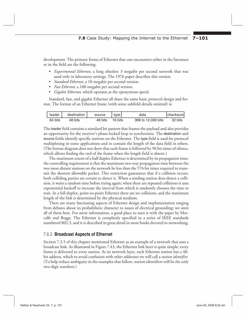
7.8 Case Study: Mapping the Internet to the Ethernet 7–101
development. The primary forms of Ethernet that one encounters either in the literature or in the field are the following:
• Experimental Ethernet, a long obsolete 3 megabit per second network that was used only in laboratory settings. The 1976 paper describes this version.
• Standard Ethernet, a 10 megabit per second version. • Fast Ethernet, a 100 megabit per second version. • Gigabit Ethernet, which operates at the eponymous speed.
Standard, fast, and gigabit Ethernet all share the same basic protocol design and format. The format of an Ethernet frame (with some subfield details omitted) is:
leader destination source type data checksum
32 bits64 bits 48 bits 48 bits 16 bits 368 to 12,000 bits
The leader field contains a standard bit pattern that frames the payload and also provides an opportunity for the receiver’s phase-locked loop to synchronize. The destination and source fields identify specific stations on the Ethernet. The type field is used for protocol multiplexing in some applications and to contain the length of the data field in others. (The format diagram does not show that each frame is followed by 96 bit times of silence, which allows finding the end of the frame when the length field is absent.)
The maximum extent of a half duplex Ethernet is determined by its propagation time; the controlling requirement is that the maximum two-way propagation time between the two most distant stations on the network be less than the 576 bit times required to transmit the shortest allowable packet. This restriction guarantees that if a collision occurs, both colliding parties are certain to detect it. When a sending station does detect a collision, it waits a random time before trying again; when there are repeated collisions it uses exponential backoff to increase the interval from which it randomly chooses the time to wait. In a full duplex, point-to-point Ethernet there are no collisions, and the maximum length of the link is determined by the physical medium.
There are many fascinating aspects of Ethernet design and implementation ranging from debates about its probabilistic character to issues of electrical grounding; we omit all of them here. For more information, a good place to start is with the paper by Metcalfe and Boggs. The Ethernet is completely specified in a series of IEEE standards numbered 802.3, and it is described in great detail in most books devoted to networking.
7.8.2 Broadcast Aspects of Ethernet
Section 7.3.5 of this chapter mentioned Ethernet as an example of a network that uses a broadcast link. As illustrated in Figure 7.43, the Ethernet link layer is quite simple: every frame is delivered to every station. At its network layer, each Ethernet station has a 48bit address, which to avoid confusion with other addresses we will call a station identifier. (To help reduce ambiguity in the examples that follow, station identifiers will be the only two-digit numbers.)
Saltzer & Kaashoek Ch. 7, p. 101 June 25, 2009 8:22 am
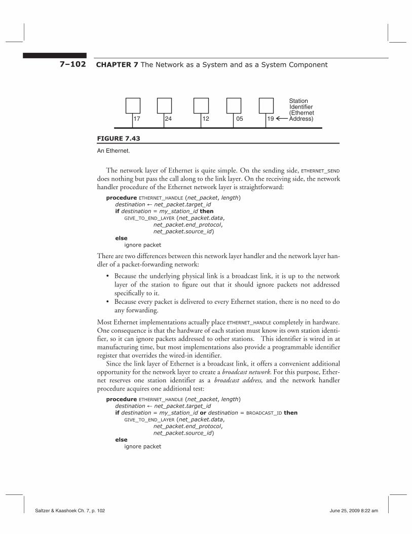
7–102 CHAPTER 7 The Network as a System and as a System Component
17 24 12 05 19
Station Identifier (Ethernet Address)
FIGURE 7.43
An Ethernet.
The network layer of Ethernet is quite simple. On the sending side, ETHERNET_SEND
does nothing but pass the call along to the link layer. On the receiving side, the network handler procedure of the Ethernet network layer is straightforward:
procedure ETHERNET_HANDLE (net_packet, length) destination ← net_packet.target_id if destination = my_station_id then
GIVE_TO_END_LAYER (net_packet.data, net_packet.end_protocol, net_packet.source_id)
else ignore packet
There are two differences between this network layer handler and the network layer handler of a packet-forwarding network:
• Because the underlying physical link is a broadcast link, it is up to the network layer of the station to figure out that it should ignore packets not addressed specifically to it.
• Because every packet is delivered to every Ethernet station, there is no need to do any forwarding.
Most Ethernet implementations actually place ETHERNET_HANDLE completely in hardware. One consequence is that the hardware of each station must know its own station identifier, so it can ignore packets addressed to other stations. This identifier is wired in at manufacturing time, but most implementations also provide a programmable identifier register that overrides the wired-in identifier.
Since the link layer of Ethernet is a broadcast link, it offers a convenient additional opportunity for the network layer to create a broadcast network. For this purpose, Ethernet reserves one station identifier as a broadcast address, and the network handler procedure acquires one additional test:
procedure ETHERNET_HANDLE (net_packet, length) destination ← net_packet.target_id if destination = my_station_id or destination = BROADCAST_ID then
GIVE_TO_END_LAYER (net_packet.data, net_packet.end_protocol, net_packet.source_id)
else ignore packet
Saltzer & Kaashoek Ch. 7, p. 102 June 25, 2009 8:22 am

7.8 Case Study: Mapping the Internet to the Ethernet 7–103
The Ethernet broadcast feature is seductive. It has led people to propose also adding broadcast features to packet-forwarding networks. It is possible to develop broadcast algorithms for a forwarding network, but it is a much trickier business. Even in Ethernet broadcast must be used judiciously. Reliable transport protocols that require that every receiving station send back an acknowledgment lead to a problematic flood of acknowledgment packets. In addition, broadcast mechanisms are too easily triggered by mistake. For example, if a request is accidentally sent with its source address set to the broadcast address, the response will be broadcast to all network attachment points. The worst case is a broadcast sent from the broadcast address, which can lead to a flood of broadcasts. Such mechanisms make a good target for malicious attack on a network, so it is usually thought to be preferable not to implement them at all.
7.8.3 Layer Mapping: Attaching Ethernet to a Forwarding Network
Suppose we have several workstations and perhaps a few servers in one building, all connected using an Ethernet, and we would like to attach this Ethernet to the packet-forwarding network illustrated in Figure 7.31 on page 7–50, by making the Ethernet a sixth link on router K in that figure. This connection produces the configuration of Figure 7.44.
There are three kinds of network-related labels in the figure. First, each link is numbered with a local single-digit link identifier (in italics), as viewed from within the station that attaches that link. Second, as in Figure 7.43, each Ethernet attachment point has a two-digit Ethernet station identifier. Finally, each station has a one-letter name, just as in the packet-forwarding network in the figure on page 7–50. With this configuration, workstation L sends a remote procedure call to server N by sending one or more packets to station 18 of the Ethernet attached to it as link number 1.
server routerwork
station work
station work
station work
station
1 61111
1
17 18 14 22 1915
… 3 2
4 5
upper-layer network address link identifier G
L M N P Q K
H
J
E
Ethernet F
Ethernet station identifier
FIGURE 7.44
Connecting an Ethernet to a packet forwarding network.
Saltzer & Kaashoek Ch. 7, p. 103 June 25, 2009 8:22 am

7–104 CHAPTER 7 The Network as a System and as a System Component
Workstation L might also want to send a request to the computer connected to the destination E, which requires that L actually send the request packet to router K at Ethernet station 19 for forwarding to destination E. The complication is that E may be at address 15 of the packet-forwarding network, while workstation M is at station 15 of the Ethernet. Since Ethernet station identifiers may be wired into the hardware interface, we probably can’t set them to suit our needs, and it might be a major hassle to go around changing addresses on the original packet-forwarding network. The bottom line here is that we can’t simply use Ethernet station identifiers as the network addresses in our packet-forwarding network. But this conclusion seems to leave station L with no way of expressing the idea that it wants to send a packet to address E.
We were able to express this idea in words because in the two figures we assigned a unique letter identifier to every station. What our design needs is a more universal concept of network—a cloud that encompasses every station in both the Ethernet and the packet-forwarding network and assigns each station a unique network address. Recall that the letter identifiers originally stood for addresses in the packet-forwarding network; they may even be hierarchical identifiers. We can simply extend that concept and assign identifiers from that same numbering plan to each Ethernet station, in addition to the wired-in Ethernet station identifiers.
What we are doing here is mapping the letter identifiers of the packet-forwarding network to the station identifiers of the Ethernet. Since the Ethernet is itself decomposable into a network layer and a link layer, we can describe this situation, as was suggested on page 7–34, as a mapping composition—an upper-level network layer is being mapped to lower-level network layer. The upper network layer is a simplified version of the Internet, so we will label it with the name “internet,” using a lower case initial letter as a reminder that it is simplified. Our internet provides us with a language in which workstation L can express the idea that it wants to send an RPC request to server E, which is located somewhere beyond the router:
NETWORK_SEND (data, length, RPC, INTERNET, E)
where E is the internet address of the server, and the fourth argument selects our internet forwarding protocol from among the various available network protocols. With this scheme, station A also uses the same network address E to send a request to that server. In other words, this internet provides a universal name space.
Our new, expanded, internet network layer must now map its addresses into the Ethernet station identifiers required by the Ethernet network layer. For example, when workstation L sends a remote procedure call to server N by
NETWORK_SEND (data, length, RPC, INTERNET, N)
the internet network layer must turn this into the Ethernet network-layer call
NETWORK_SEND (data, length, RPC, ENET, 18)
in which we have named the Ethernet network-layer protocol ENET.
Saltzer & Kaashoek Ch. 7, p. 104 June 25, 2009 8:22 am
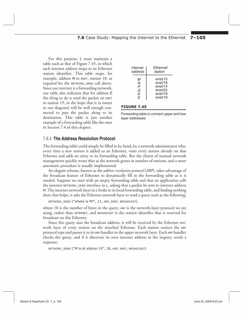
7.8 Case Study: Mapping the Internet to the Ethernet 7–105
For this purpose, L must maintain a table such as that of Figure 7.45, in which each internet address maps to an Ethernet station identifier. This table maps, for example, address N to ENET, station 18, as required for the NETWORK_SEND call above. Since our internet is a forwarding network, our table also indicates that for address E the thing to do is send the packet on ENET
to station 19, in the hope that it (a router in our diagram) will be well enough connected to pass the packet along to its destination. This table is just another example of a forwarding table like the ones in Section 7.4 of this chapter.
7.8.4 The Address Resolution Protocol
internet address
M N P Q K E
Ethernet/ station
enet/15 enet/18 enet/14 enet/22 enet/19 enet/19
FIGURE 7.45
Forwarding table to connect upper and lowe layer addresses
The forwarding table could simply be filled in by hand, by a network administrator who, every time a new station is added to an Ethernet, visits every station already on that Ethernet and adds an entry to its forwarding table. But the charm of manual network management quickly wears thin as the network grows in number of stations, and a more automatic procedure is usually implemented.
An elegant scheme, known as the address resolution protocol (ARP), takes advantage of the broadcast feature of Ethernet to dynamically fill in the forwarding table as it is needed. Suppose we start with an empty forwarding table and that an application calls the internet NETWORK_SEND interface in L, asking that a packet be sent to internet address M. The internet network layer in L looks in its local forwarding table, and finding nothing there that helps, it asks the Ethernet network layer to send a query such as the following:
NETWORK_SEND (“where is M?”, 11, ARP, ENET, BROADCAST)
where 10 is the number of bytes in the query, ARP is the network-layer protocol we are using, rather than INTERNET, and BROADCAST is the station identifier that is reserved for broadcast on this Ethernet.
Since this query uses the broadcast address, it will be received by the Ethernet network layer of every station on the attached Ethernet. Each station notices the ARP
protocol type and passes it to its ARP handler in the upper network layer. Each ARP handler checks the query, and if it discovers its own internet address in the inquiry, sends a response:
NETWORK_SEND (“M is at station 15”, 18, ARP, ENET, BROADCAST)
Saltzer & Kaashoek Ch. 7, p. 105 June 25, 2009 8:22 am

7–106 CHAPTER 7 The Network as a System and as a System Component
At most, one station—the one whose internet address is named by the ARP request—will respond. All the others will internet Ethernet/
stationignore the ARP request. When the ARP response arrives at sta- address
tion 17, that station’s Ethernet network layer will pass it up M enet/15 to the ARP handler in its upper network layer, which will immediately add an entry relating address M to station 15 to its forwarding table, shown at the right. The internet network handler of station 17 can now proceed with its originally requested send operation.
Suppose now that station L tries to send a packet to server
internet Ethernet/ E, which is on the internet but not directly attached to the
station Ethernet. In that case, server E does not hear the Ethernetaddress broadcast, but the router at station 19 does, and it sends a
M enet/15 suitable ARP response instead. The forwarding table thenE enet/19
has a second entry as shown at the left. Station L can now send the packet to the router, which presumably knows
how to forward the packet to its intended destination. One more step is required—the server at E will not be able to reply to station L unless
L is in its own forwarding table. This step is easy to arrange: whenever router K hears, via ARP, of the existence of a station on its attached Ethernet, it simply adds that internet address to the list of addresses that it advertises, and whatever routing protocol it is using will propagate that information throughout the internet. If hierarchical addresses are in use, the region designer might assign a region number to be used exclusively for all the stations on one Ethernet, to simplify routing.
Mappings from Ethernet station identifiers to the addresses of the higher network level are thus dynamically built up, and eventually station L will have the full table shown in Figure 7.45. Typical systems deployed in the field have developed and refined this basic set of dynamic mapping ideas in many directions: The forwarding table is usually managed as a cache, with entries that time out or can be explicitly updated, to allow stations to change their station identifiers; the ARP response may also be noted by stations that didn’t send the original ARP request for their own future reference; a newly-attached station may, without being asked, broadcast what appears to be an ARP response simply to make itself known to existing stations (advertising); and there is even a reverse version of the ARP protocol that can be used by a station to ask if anyone knows its own higher-level network address, or to ask that a higher-level address be assigned to it. These refinements are not important to our case study, but many of them are essential to smooth network management.
Saltzer & Kaashoek Ch. 7, p. 106 June 25, 2009 8:22 am

7.9 War Stories: Surprises in Protocol Design 7–107
7.9 War Stories: Surprises in Protocol Design
7.9.1 Fixed Timers Lead to Congestion Collapse in NFS
A classic example of congestion collapse appeared in early releases of the Sun Network File System (NFS) described in the case study in Section 4.5. The NFS server implemented at-least-once semantics with an idempotent stateless interface. The NFS client was programmed to be persistent. If it did not receive a response after some fixed number of seconds, it would resend its request, repeating forever, if necessary. The server simply ran a first-in, first-out queue, so if several NFS clients happened to make requests of the server at about the same time, the server would handle the requests one at a time in the order that they arrived. These apparently plausible arrangements on the parts of the client and the server, respectively, set the stage for the problem.
As the number of clients increased, the length of the queue increased accordingly. With enough clients, the queue would grow long enough that some requests would time out before the server got to them. Those clients, upon timing out, would repeat their requests. In due course, the server would handle the original request of a client that had timed out, send a response, and that client would go away happy. But that client’s duplicate request was still in the server’s queue. The stateless NFS server had no way to tell that it had already handled the duplicate request, so when it got to the duplicate it would go ahead and handle it again, taking the same time as before, and sending an unneeded response. The client ignored this response, but the time spent by the server handling the duplicate request was wasted, and the waste occurred at a time when the server could least afford it—it was already so heavily loaded that at least one client had timed out.
Once the server began wasting time handling duplicate requests, the queue grew still longer, causing more clients to time out, leading to more duplicate requests. The observed effect was that a steady increase of load would result in a steady increase of satisfied requests, up to the point that the server was near full capacity. If the load ever exceeded the capacity, even for a short time, every request from then on would time out, and be duplicated, resulting in a doubling of the load on the server. That wasn’t the end—with a doubled load, clients would begin to time out a second time, send their requests yet again, thus tripling the load. From there, things would continue to deteriorate, with no way to recover.
From the NFS server’s point of view, it was just doing what its clients were asking, but from the point of view of the clients the useful throughput had dropped to zero. The solution to this problem was for the clients to switch to an exponential backoff algorithm in their choice of timer setting: each time a client timed out it would double the size of its timer setting for the next repetition of the request.
Lesson: Fixed timers are always a source of trouble, sometimes catastrophic trouble.
Saltzer & Kaashoek Ch. 7, p. 107 June 25, 2009 8:22 am

7–108 CHAPTER 7 The Network as a System and as a System Component
7.9.2 Autonet Broadcast Storms
Autonet, an experimental local area network designed at the Digital Equipment Corporation Systems Research Center, handled broadcast in an elegant way. The network was organized as a tree. When a node sent a packet to the broadcast address, the network first routed the packet up to the root of the tree. The root turned the packet around and sent it down every path of the tree. Nodes accepted only packets going downward, so this procedure ensured that a broadcast packet would reach every connected node, but no more than once. But every once in a while, the network collapsed with a storm of repeated broadcast packets. Analysis of the software revealed no possible source of the problem. It took a hardware expert to figure it out.
The physical layer of the Autonet consisted of point-to-point coaxial cables. An interesting property of an unterminated coaxial cable is that it will almost perfectly reflect any signal sent down the cable. The reflection is known as an “echo”. Echos are one of the causes of ghosts in analog cable television systems.
In the case of the Autonet, the network card in each node properly terminated the cable, eliminating echos. But if someone disconnected a computer from the network, and left the cable dangling, that cable would echo everything back to its source.
Suppose someone disconnects a cable, and someone else in the network sends a packet to the broadcast address. The network routes the packet up to the root of the tree, the root turns the packet around and sends it down the tree. When the packet hits the end of the unterminated cable, it reflects and returns to the other end of the cable looking like a new upward bound packet with the broadcast address. The node at that end dutifully forwards the packet toward the root node, which, upon receipt turns it around and sends it again. And again, and again, as fast as the network can carry the packet.
Lesson: Emergent properties often arise from the interaction of apparently unrelated system features operating at different system layers, in this case, link-layer reflections and network-layer broadcasts.
7.9.3 Emergent Phase Synchronization of Periodic Protocols
Some network protocols involve periodic polling. Examples include picking up mail, checking for chat buddies, and sending “are-you-there?” inquiries for reassurance that a co-worker hasn’t crashed. For a specific example, a workstation might send a broadcast packet every five minutes to announce that it is still available for conversations. If there are dozens of such workstations on the same local area network, the designer would prefer that they not all broadcast simultaneously. One might assume that, even if they all broadcast with the same period, if they start at random their broadcasts would be out of phase and it would take a special effort to synchronize their phases and keep them that way. Unfortunately, it is common to discover that they have somehow synchronized themselves and are all trying to broadcast at the same time.
How can this be? Suppose, for example, that each one of a group of workstations sends a broadcast and then sets a timer for a fixed interval. When the timer expires, it
Saltzer & Kaashoek Ch. 7, p. 108 June 25, 2009 8:22 am
7.9 War Stories: Surprises in Protocol Design 7–109
sends another broadcast and, after sending, it again sets the timer. During the time that it is sending the broadcast message, the timer is not running. If a second workstation happens to send a broadcast during that time, both workstations take a network interrupt, each accepts the other station’s broadcast, and makes a note of it, as might be expected. But the time required to handle the incoming broadcast interrupts slightly delays the start of the next timing cycle for both of the workstations, whereas broadcasts that arrive while a workstation’s timer is running don’t affect the timer. Although the delay is small, it does shift the timing of these workstation’s broadcasts relative to all of the other workstations. The next time this workstation’s timer expires, it will again be interrupted by the other workstation, since they are both using the same timer value, and both of their timing cycles will again be slightly lengthened. The two workstations have formed a phase-locked group, and will remain that way indefinitely.
More important, the two workstations that were accidentally synchronized are now polling with a period that is slightly larger than all the other workstations. As a result, their broadcasts now precess relative to the others, and eventually will overlap the time of broadcast of a third workstation. That workstation will then join the phase-locked group, increasing the rate of precession, and things continue from there. The problem is that the system design unintentionally includes an emergent phase-locked loop, similar to the one described on page 7–36.
The generic mechanism is that the supposed “fixed” interval does not count the running time of the periodic program, and that for some reason that running time is different when two or more participants happen to run concurrently. In a network, it is quite common to find that unsynchronized activities with identical timing periods become synchronized.
Lesson: Fixed timers have many evils. Don’t assume that unsynchronized periodic activities will stay that way.
7.9.4 Wisconsin Time Server Meltdown
NE TGEAR®, a manufacturer of Ethernet and wireless equipment, added a feature to four of its low-cost wireless routers intended for home use: a log of packets that traverse the router. To be useful in debugging, the designers realized that the log needed to timestamp each log entry, but adding timestamps required that the router know the current date and time. Since the router would be attached to the Internet, the designers added a few lines of code that invoked a simple network time service protocol known as SNTP. Since SNTP requires that the client invoke a specific time service, there remained a name discovery problem. They solved it by configuring the firmware code with the Internet address of a network time service. Specifically, they inserted the address 128.105.39.11, the network address of one of the time servers operated by the University of Wisconsin. The designers surrounded this code with a persistent sender that would retry the protocol once per second until it received a response. Upon receiving a response, it refreshed the clock with another invocation of SNTP, using the same persistent sender, on a schedule ranging from once per minute to once per day, depending on the firmware version.
Saltzer & Kaashoek Ch. 7, p. 109 June 25, 2009 8:22 am
7–110 CHAPTER 7 The Network as a System and as a System Component
On May 14, 2003, at about 8:00 a.m. local time, the network staff at the University of Wisconsin noticed an abrupt increase in the rate of inbound Internet traffic at their connection to the Internet—the rate jumped from 20,000 packets per second to 60,000 packets per second. All of the extra traffic seemed to be SNTP packets targeting one of their time servers, and specifying the same UDP response port, port 23457. To prevent disruption to university network access, the staff installed a temporary filter at their border routers that discarded all incoming SNTP request packets that specified a response port of 23457. They also tried invoking an SNTP protocol access control feature in which the service can send a response saying, in effect, “go away”, but it had no effect on the incoming packet flood.
Over the course of the next few weeks, SNTP packets continued to arrive at an increasing rate, soon reaching around 270,000 packets per second, and consuming about 150 megabits per second of Internet connection capacity. Analysis of the traffic showed that the source addresses seemed to be legitimate and that any single source was sending a packet about once per second. A modest amount of sleuthing identified the NETGEAR routers as the source of the packets and the firmware as containing the target address and response port numbers. Deeper analysis established that the immediate difficulty was congestion collapse. NETGEAR had sold over 700,000 routers containing this code world-wide. As the number in operation increased, the load on the Wisconsin time service grew gradually until one day the response latency of the server exceeded one second. At that point, the NETGEAR router that made that request timed out and retried, thereby increasing its load on the time service, which increased the time service response latency for future requesters. After a few such events, essentially all of the NETGEAR routers would start to time out, thereby multiplying the load they presented by a factor of 60 or more, which ensured that the server latency would continue to exceed their one second timer.
How Wisconsin and NETGEAR solved this problem, and at whose expense, is a whole separate tale.*
Lesson(s): There are several. (1) Fixed timers were once again found at the scene of an accident. (2) Configuring a fixed Internet address, which is overloaded with routing information, is a bad idea. In this case, the wired-in address made it difficult to repair the problem by rerouting requests to a different time service, such as one provided by NETGEAR. The address should have been a variable, preferably one that could be hidden with indirection (decouple modules with indirection). (3) There is a reason for features such as the “go away” response in SNTP; it is risky for a client to implement only part of a protocol.
* For that story, see <http://www.cs.wisc.edu/~plonka/netgear-sntp/>. This incident is also described in David Mills, Judah Levine, Richard Schmidt and David Plonka. “Coping with overload on the Network Time Protocol public servers.” Proceedings of the Precision Time and Time Interval (PTTI) Applications and Planning Meeting (Washington DC, December 2004), pages 5-16.
Saltzer & Kaashoek Ch. 7, p. 110 June 25, 2009 8:22 am

Exercises 7–111
Exercises
7.1 Chapter 1 discussed four general methods for coping with complexity: modularity, abstraction, hierarchy, and layering. Which of those four methods does a protocol stack use as its primary organizing scheme?
1996–1–1e
7.2 The end-to-end argument
A. is a guideline for placing functions in a computer system; B. is a rule for placing functions in a computer system; C. is a debate about where to place functions in a computer system; D. is a debate about anonymity in computer networks.
1999–2–03
7.3 Of the following, the best example of an end-to-end argument is:
A. If you laid all the Web hackers in the world end to end, they would reach from Cambridge to CERN.
B. Every byte going into the write end of a UNIX pipe eventually emerges from the pipe’s read end.
C. Even if a chain manufacturer tests each link before assembly, he’d better test the completed chain.
D. Per-packet checksums must be augmented by a parity bit for each byte. E. All important network communication functions should be moved to the application
layer. 1998–2–01
7.4 Give two scenarios in the form of timing diagrams showing how a duplicate request might end up at a service.
1995-1-5a
7.5 After sending a frame, a certain piece of network software waits one second for an acknowledgment before retransmitting the frame. After each retransmission, it cuts delay in half, so after the first retransmission the wait is 1/2 second, after the second retransmission the wait is 1/4 second, etc. If it has reduced the delay to 1/1024
Saltzer & Kaashoek Ch. 7, p. 111 June 25, 2009 8:22 am
7–112 CHAPTER 7 The Network as a System and as a System Component
second without receiving an acknowledgment, the software gives up and reports to its caller that it was not able to deliver the frame.
7.5a. Is this a good way to manage retransmission delays for Ethernet? Why or why not? 1987–1–2a
7.5b. Is this a good way to manage retransmission delays for a receive-and-forward network? Why or why not?
1987–1–2b
7.6 Variable delay is an intrinsic problem of isochronous networks. True or False? 1995–1–1f
7.7 Host A is sending frames to host B over a noisy communication link. The median transit time over the communication link is 100 milliseconds. The probability of a frame being damaged en route in either direction across the communication link is α, and B can reliably detect the damage. When B gets a damaged frame it simply discards it. To ensure that frames arrive safely, B sends an acknowledgment back to A for every frame received intact.
7.7a. How long should A wait for a frame to be acknowledged before retransmitting it? 1987–1–3a
7.7b. What is the average number of times that A will have to send each frame? 1987–1–3b
7.8 Consider the protocol reference model of this chapter with the link, network, and end-to-end layers. Which of the following is a behavior of the reference model?
A. An end-to-end layer at an end host tells its network layer which network layer protocol to use to reach a destination.
B. The network layer at a router maintains a separate queue of packets for each end-toend protocol.
C. The network layer at an end host looks at the end-to-end type field in the network header to decide which end-to-end layer protocol handler to invoke.
D. The link layer retransmits packets based on the end-to-end type of the packets: if the end-to-end protocol is reliable, then a link-layer retransmission occurs when a loss is detected at the link layer, otherwise not.
2000–2–02
Saltzer & Kaashoek Ch. 7, p. 112 June 25, 2009 8:22 am

Exercises 7–113
7.9 Congestion is said to occur in a receive-and-forward network when A. Communication stalls because of cycles in the flow-control dependencies. B. The throughput demanded of a network link exceeds its capacity. C. The volume of e-mail received by each user exceeds the rate at which users can read
e-mail. D. The load presented to a network link persistently exceeds its capacity. E. The amount of space required to store routing tables at each node becomes
burdensome. 1997–1–1e
7.10 Alice has arranged to send a stream of data to Bob using the following protocol:
• Each message segment has a block number attached to it; block numbers are consecutive starting with 1.
• Whenever Bob receives a segment of data with the number N he sends back an acknowledgment saying “OK to send block N + 1”.
• Whenever Alice receives an “OK to send block K” she sends block K.
Alice initiates the protocol by sending a block numbered 1, she terminates the protocol by ignoring any “OK to send block K” for which K is larger than the number on the last block she wants to send. The network has been observed to never lose message segments, so Bob and Alice have made no provision for timer expirations and retries. They have also made no provision for deduplication. Unfortunately, the network systematically delivers every segment twice. Alice starts the protocol, planning to send a three-block stream. How many “OK to send block 4” responses does she ignore at the end?
1994–2–6
7.11 A and B agree to use a simple window protocol for flow control for data going from A to B: When the connection is first established, B tells A how many message segments B can accept, and as B consumes the segments it occasionally sends a message to A saying “you can send M more”. In operation, B notices that occasionally A sends more segments than it was supposed to. Explain.
1980–3–3
7.12 Assume a client and a service are directly connected by a private, 800,000 bytes per second link. Also assume that the client and the service produce and consume
Saltzer & Kaashoek Ch. 7, p. 113 June 25, 2009 8:22 am
7–114 CHAPTER 7 The Network as a System and as a System Component
message segments at the same rate. Using acknowledgments, the client measures the round-trip between itself and the service to be 10 milliseconds.
7.12a. If the client is sending message segments that require 1000-byte frames, what is the smallest window size that allows the client to achieve 800,000 bytes per second throughput?
1995–2–2a
7.12b. One scheme for establishing the window size is similar to the slow start congestion control mechanism. The idea is that the client starts with a window size of one. For every segment received, the service responds with an acknowledgment telling the client to double the window size. The client does so until it realizes that there is no point in increasing it further. For the same parameters as in part 7.12a, how long would it take for the client to realize it has reached the maximum throughput?
1995–2–2b
7.12c. Another scheme for establishing the window size is called fast start. In (an oversimplified version of ) fast start, the client simply starts sending segments as fast as it can, and watches to see when the first acknowledgment returns. At that point, it counts the number of outstanding segments in the pipeline, and sets the window size to that number. Again using the same parameters as in part 7.12a, how long will it take for the client to know it has achieved the maximum throughput?
1995–2–2c
7.13 A satellite in stationary orbit has a two-way data channel that can send frames containing up to 1000 data bytes in a millisecond. Frames are received without error after 249 milliseconds of propagation delay. A transmitter T frequently has a data file that takes 1000 of these maximal-length frames to send to a receiver R. T and R start using lock-step flow control. R allocates a buffer which can hold one message segment. As soon as the buffered segment is used and the buffer is available to hold new data, R sends an acknowledgment of the same length. T sends the next segment as soon as it sees the acknowledgment for the last one.
7.13a. What is the minimum time required to send the file? 1988–2–2a
7.13b. T and R decide that lock-step is too slow, so they change to a bang-bang protocol. A bang-bang protocol means that R sends explicit messages to T saying “go ahead” or “pause”. The idea is that R will allocate a receive buffer of some size B, send a go-ahead message when it is ready to receive data. T then sends data segments as fast as the channel can absorb them. R sends a pause message at just the right time so that its buffer will not overflow even if R stops consuming message segments.
Saltzer & Kaashoek Ch. 7, p. 114 June 25, 2009 8:22 am
Exercises 7–115
Suppose that R sends a go-ahead, and as soon as it sees the first data arrive it sends a pause. What is the minimum buffer size Bmin that it needs?)
1988–2–2b]
7.13c. What now is the minimum time required to send the file? 1988–2–2c
7.14 Some end-to-end protocols include a destination field in the end-to-end header. Why?
A. So the protocol can check that the network layer routed the packet containing the message segment correctly.
B. Because an end-to-end argument tells us that routing should be performed at the end-to-end layer.
C. Because the network layer uses the end-to-end header to route the packet. D. Because the end-to-end layer at the sender needs it to decide which network protocol
to use. 2000–2–09
7.15 One value of hierarchical naming of network attachment points is that it allows a reduction in the size of routing tables used by packet forwarders. Do the packet forwarders themselves have to be organized hierarchically to take advantage of this space reduction?
1994–2–5
7.16 The System Network Architecture (SNA) protocol family developed by IBM uses a flow control mechanism called pacing. With pacing, a sender may transmit a fixed number of message segments, and then must pause. When the receiver has accepted all of these segments, it can return a pacing response to the sender, which can then send another burst of message segments.
Suppose that this scheme is being used over a satellite link, with a delay from earth station to earth station of 250 milliseconds. The frame size on the link is 1000 bits, four segments are sent before pausing for a pacing response, and the satellite channel has a data rate of one megabit per second.
7.16a. The timing diagram below illustrates the frame carrying the first segment. Fill in the diagram to show the next six frames exchanged in the pacing system. Assume no frames are lost, delays are uniform, and sender and receiver have no internal
Saltzer & Kaashoek Ch. 7, p. 115 June 25, 2009 8:22 am

7–116 CHAPTER 7 The Network as a System and as a System Component
delays (for example, the first bit of the second frame may immediately follow the last bit of the first).
sender receiver
time, in ms 0 1
250 251
first bit of first frame leaves sender last bit of first frame leaves sender
first bit of first frame arrives at receiver last bit of first frame arrives at receiver
7.16b. What is the maximum fraction of the available satellite capacity that can be used by this pacing scheme?
7.16c. We would like to increase the utilization of the channel to 50% but we can't increase the frame size. How many message segments would have to be sent between pacing responses to achieve this capacity?
1982–3–4
7.17 Which are true statements about network address translators as described in Section 7.4.5?
A. NATs break the universal addressing scheme of the Internet. B. NATs break the layering abstraction of the network model of Chapter 7. C. NATs increase the consumption of Internet addresses. D. NATs address the problem that the Internet has a shortage of Internet addresses. E. NATs constrain the design of new end-to-end protocols. F. When a NAT translates the Internet address of a packet, it must also modify the
Ethernet checksum, to ensure that the packet is not discarded by the next router that handles it. The client application might be sending its Internet address in the TCP payload to the server.
G. When a packet from the public Internet arrives at a NAT box for delivery to a host behind the NAT, the NAT must examine the payload and translate any Internet addresses found therein.
H. Clients behind a NAT cannot communicate with servers that are behind the same NAT because the NAT does not know how to forward those packets.
2001–2–01, 2002–2–02, and 2004–2–2
Saltzer & Kaashoek Ch. 7, p. 116 June 25, 2009 8:22 am
Exercises 7–117
7.18 Some network protocols deal with both big-endian and little-endian clients by providing two different network ports. Big-endian clients send requests and data to one port, while little-endian clients send requests and data to the other. The service may, of course, be implemented on either a big-endian or a little-endian machine. This approach is unusual—most Internet protocols call for just one network port, and require that all data be presented at that port in “network standard form”, which is little- endian. Explain the advantage of the two port structure as compared with the usual structure.
1994–1–2
7.19 Ethernet cannot scale to large sizes because a centralized mechanism is used to control network contention. True or False?
1994–1–3b
7.20 Ethernet
A. uses luminiferous ether to carry packets. B. uses Manchester encoding to frame bits. C. uses exponential back-off to resolve repeated conflicts between multiple senders. D. uses retransmissions to avoid congestion. E. delegates arbitration of conflicting transmissions to each station. F. always guarantees the delivery of packets. G. can support an unbounded number of computers. H. has limited physical range.
1999–2–01, 2000–1–04
7.21 Ethernet cards have unique addresses built into them. What role do these unique addresses play in the Internet?
A. None. They are there for Macintosh compatibility only. B. A portion of the Ethernet address is used as the Internet address of the computer
using the card. C. They provide routing information for packets destined to non-local subnets. D. They are used as private keys in the Security Layer of the ISO protocol. E. They provide addressing within each subnet for an Internet address resolution
protocol. F. They provide secure identification for warranty service.
1998-2-02
7.22 If eight stations on an Ethernet all want to transmit one packet, which of the following statements is true?
Saltzer & Kaashoek Ch. 7, p. 117 June 25, 2009 8:22 am
7–118 CHAPTER 7 The Network as a System and as a System Component
A. It is guaranteed that all transmissions will succeed. B. With high probability all stations will eventually end up being able to transmit their
data successfully. C. Some of the transmissions may eventually succeed, but it is likely some may not. D. It is likely that none of the transmissions will eventually succeed.
2004–1–3
7.23 Ben Bitdiddle has been thinking about remote procedure call. He remembers that one of the problems with RPC is the difficulty of passing pointers: since pointers are really just addresses, if the service dereferences a client pointer, it’ll get some value from its address space, rather than the intended value in the client’s address space. Ben decides to redesign his RPC system to always pass, in the place of a bare pointer, a structure consisting of the original pointer plus a context reference. Louis Reasoner, excited by Ben’s insight, decides to change all end-to-end protocols along the same lines. Argue for or against Louis’s decision.
1996–2–1a
7.24 Alyssa’s mobiles:* Alyssa P. Protocol-Hacker is designing an end-to-end protocol for locating mobile hosts. A mobile host is a computer that plugs into the network at different places at different times, and get assigned a new network address at each place. The system she starts with assigns each host a home location, which can be found simply by looking the user up in a name service. Her end-to-end protocol will use a network that can reorder packets, but doesn’t ever lose or duplicate them. Her first protocol is simple: every time a user moves, store a forwarding pointer at the previous location, pointing to the new location. This creates a chain of forwarding pointers with the permanent home location at the beginning and the mobile host at the end. Packets meant for the mobile host are sent to the home location, which forwards them along the chain until they reach the mobile host itself. (The chain is truncated when a mobile host returns to a previously visited location.) Alyssa notices that because of the long chains of forwarding pointers, performance generally gets worse each time she moves her mobile host. Alyssa’s first try at fixing the problem works like this: Each time a mobile host moves, it sends a message to its home location indicating its new location. The home location maintains a pointer to the new location. With this protocol, there are no chains at all. Places other than the home location do not maintain forwarding information.
7.24a. When this protocol is implemented, Alyssa notices that packets regularly get lost when she moves from one location to another. Explain why or give an example.
\
Alyssa is disappointed with her first attempt, and decides to start over. In her new scheme, no forwarding pointers are maintained anywhere, not even at the home
* Credit for developing exercise 7.24 goes to Anant Agarwal.
Saltzer & Kaashoek Ch. 7, p. 118 June 25, 2009 8:22 am
Exercises 7–119
node. Say a packet destined for a mobile host A arrives at a node N. If N can directly communicate with A, then N sends the packet to A, and we’re done. Otherwise, N broadcasts a search request for A to all the other fixed nodes in the network. If A is near a different fixed node N', then N' responds to the search request. On receiving this response, N forwards the packet for A to N'.
7.24b. Will packets get lost with this protocol, even if A moves before the packet gets to N'? Explain.
Unfortunately the network doesn’t support broadcast efficiently, so Alyssa goes back to the keyboard and tries again. Her third protocol works like this. Each time a mobile host moves, say from N to N', a forwarding pointer is stored at N pointing to N'. Every so often, the mobile host sends a message to its permanent home node with its current location. Then, the home node propagates a message down the forwarding chain, asking the intermediate nodes to delete their forwarding state.
7.24c. Can Alyssa ever lose packets with this protocol? Explain. (Hint: think about the properties of the underlying network.)
7.24d. What additional steps can the home node take to ensure that the scheme in question 7.24c never loses packets?
1996–2–2
7.25 ByteStream Inc. sells three data-transfer products: Send-and-wait, Blast, and Flow-control. Mike R. Kernel is deciding which product to use. The protocols work as follows:
• Send-and-wait sends one segment of a message and then waits for an acknowledgment before sending the next segment.
• Flow-control uses a sliding window of 8 segments. The sender sends until the window closes (i.e., until there are 8 unacknowledged segments). The receiver sends an acknowledgment as soon as it receives a segment. Each acknowledgment opens the sender’s window with one segment.
• Blast uses only one acknowledgment. The sender blasts all the segments of a message to the receiver as fast as the network layer can accept them. The last segment of the blast contains a bit indicating that it is the last segment of the message. After sending all segments in a single blast, the sender waits for one acknowledgment from the receiver. The receiver sends an acknowledgment as soon as it receives the last segment.
Mike asks you to help him compute for each protocol its maximum throughput. He is planning to use a 1,000,000 bytes per second network that has a packet size of 1,000 bytes. The propagation time from the sender to the receiver is 500 microseconds. To simplify the calculation, Mike suggests making the following approximations: (1) there is no processing time at the sender and the receiver; (2) the time to send an acknowledgment is just the propagation time (number of data
Saltzer & Kaashoek Ch. 7, p. 119 June 25, 2009 8:22 am

7–120 CHAPTER 7 The Network as a System and as a System Component
bytes in an ACK is zero); (3) the data segments are always 1,000 bytes; and (4) all headers are zero-length. He also assumes that the underlying communication medium is perfect (frames are not lost, frames are not duplicated, etc.) and that the receiver has unlimited buffering.
7.25a. What is the maximum throughput for the Send-and-wait?
7.25b. What is the maximum throughput for Flow-control?
7.25c. What is the maximum throughput for Blast?
Mike needs to choose one of the three protocols for an application which periodically sends arbitrary-sized messages. He has a reliable network, but his application involves unpredictable computation times at both the sender and the receiver. And this time the receiver has a 20,000-byte receive buffer.
7.25d. Which product should he choose for maximum reliable operation?
A. Send-and-wait, the others might hang. B. Blast, which outperforms the others. C. Flow-control, since Blast will be unreliable and Send-and-wait is slower. D. There is no way to tell from the information given.
1997–2–2
7.26 Suppose the longest packet you can transmit across the Internet can contain 480 bytes of useful data, you are using a lock-step end-to-end protocol, and you are sending data from Boston to California. You have measured the round-trip time and found that it is about 100 milliseconds.
7.26a. If there are no lost packets, estimate the maximum data rate you can achieve.
7.26b. Unfortunately, 1% of the packets are getting lost. So you install a resend timer, set to 1000 milliseconds. Estimate the data rate you now expect to achieve.
7.26c. On Tuesdays the phone company routes some westward-bound packets via satellite link, and we notice that 50% of the round trips now take exactly 100 extra milliseconds. What effect does this delay have on the overall data rate when the resend timer is not in use. (Assume the network does not lose any packets.)
7.26d. Ben turns on the resend timer, but since he hadn’t heard about the satellite delays he sets it to 150 milliseconds. What now is the data rate on Tuesdays? (Again, assume the network does not lose any packets.)
7.26e. Usually, when discussing end-to-end data rate across a network, the first parameter one hears is the data rate of the slowest link in the network. Why wasn't that parameter needed to answer any of the previous parts of this question?
1994–1–5
Saltzer & Kaashoek Ch. 7, p. 120 June 25, 2009 8:22 am
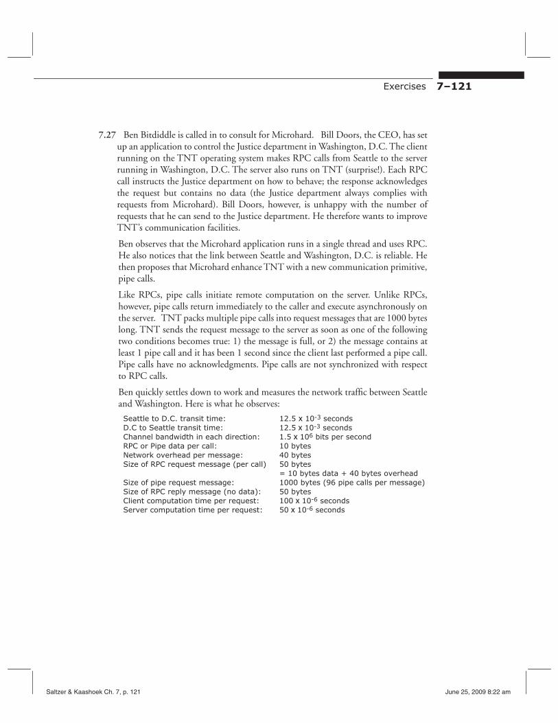
Exercises 7–121
7.27 Ben Bitdiddle is called in to consult for Microhard. Bill Doors, the CEO, has set up an application to control the Justice department in Washington, D.C. The client running on the TNT operating system makes RPC calls from Seattle to the server running in Washington, D.C. The server also runs on TNT (surprise!). Each RPC call instructs the Justice department on how to behave; the response acknowledges the request but contains no data (the Justice department always complies with requests from Microhard). Bill Doors, however, is unhappy with the number of requests that he can send to the Justice department. He therefore wants to improve TNT’s communication facilities.
Ben observes that the Microhard application runs in a single thread and uses RPC. He also notices that the link between Seattle and Washington, D.C. is reliable. He then proposes that Microhard enhance TNT with a new communication primitive, pipe calls.
Like RPCs, pipe calls initiate remote computation on the server. Unlike RPCs, however, pipe calls return immediately to the caller and execute asynchronously on the server. TNT packs multiple pipe calls into request messages that are 1000 bytes long. TNT sends the request message to the server as soon as one of the following two conditions becomes true: 1) the message is full, or 2) the message contains at least 1 pipe call and it has been 1 second since the client last performed a pipe call. Pipe calls have no acknowledgments. Pipe calls are not synchronized with respect to RPC calls.
Ben quickly settles down to work and measures the network traffic between Seattle and Washington. Here is what he observes:
Seattle to D.C. transit time: 12.5 x 10⁻³ seconds D.C to Seattle transit time: 12.5 x 10⁻³ seconds Channel bandwidth in each direction: 1.5 x 106 bits per second RPC or Pipe data per call: 10 bytes Network overhead per message: 40 bytes Size of RPC request message (per call) 50 bytes
= 10 bytes data + 40 bytes overhead Size of pipe request message: 1000 bytes (96 pipe calls per message) Size of RPC reply message (no data): 50 bytes Client computation time per request: 100 x 10-6 seconds Server computation time per request: 50 x 10-6 seconds
Saltzer & Kaashoek Ch. 7, p. 121 June 25, 2009 8:22 am
7–122 CHAPTER 7 The Network as a System and as a System Component
The Microhard application is the only one sending messages on the link.
7.27a. What is the transmission delay the client thread observes in sending an RPC request message)?
7.27b. Assuming that only RPCs are used for remote requests, what is the maximum number of RPCs per second that will be executed by this application?
7.27c. Assuming that all RPC calls are changed to pipe calls, what is the maximum number of pipe calls per second that will be executed by this application?
7.27d. Assuming that every pipe call includes a serial number argument, and serial numbers increase by one with every pipe call, how could you know the last pipe call was executed?
A. Ensure that serial numbers are synchronized to the time of day clock, and wait at the client until the time of the last serial number.
B. Call an RPC both before and after the pipe call, and wait for both calls to return. C. Call an RPC passing as an argument the serial number that was sent on the last pipe
call, and design the remote procedure called to not return until a pipe call with a given serial number had been processed.
D. Stop making pipe calls for twice the maximum network delay, and reset the serial number counter to zero.
1998–1–2a…d
7.28 Alyssa P. Hacker is implementing a client/service spell checker in which a network will stand between the client and the service. The client scans an ASCII file, sending each word to the service in a separate message. The service checks each word against its database of correctly spelled words and returns a one-bit answer. The client displays the list of incorrectly spelled words.
7.28a. The client’s cost for preparing a message to be sent is 1 millisecond, regardless of length. The network transit time is 10 milliseconds, and network data rate is infinite. The service can look up a word and determine whether or not it is misspelled in 100 microseconds. Since the service runs on a supercomputer, its cost for preparing a message to be sent is zero milliseconds. Both the client and service can receive messages with no overhead. How long will Alyssa’s design take to spell check a 1,000 word file if she uses RPC for communication (ignore acknowledgments to requests and replies, and assume that messages are not lost or reordered)?
7.28b. Alyssa does the same computations that you did and decides that the design is too slow. She decides to group several words into each request. If she packs 10 words in each request, how long will it take to spell check the same file?
7.28c. Alyssa decides that grouping words still isn’t fast enough, so she wants to know how long it would take if she used an asynchronous message protocol (with
Saltzer & Kaashoek Ch. 7, p. 122 June 25, 2009 8:22 am

Exercises 7–123
grouping words) instead of RPC. How long will it take to spell check the same file? (For this calculation, assume that messages are not lost or reordered.)
7.28d. Alyssa is so pleased with the performance of this last design that she decides to use it (without grouping) for a banking system. The service maintains a set of accounts and processes requests to debit and credit accounts (i.e., modify account balances). One day Alyssa deposits $10,000 and transfers it to Ben’s account immediately afterwards. The transfer fails with a reply saying she is overdrawn. But when she checks her balance afterwards, the $10,000 is there! Draw a time diagram explaining these events.
1996–1–4a…d
Additional exercises relating to Chapter 7 can be found in problem sets 17 through 25.
Saltzer & Kaashoek Ch. 7, p. 123 June 25, 2009 8:22 am

7–124 CHAPTER 7 The Network as a System and as a System Component
Saltzer & Kaashoek Ch. 7, p. 124 June 25, 2009 8:22 am

CHAPTERGlossary for Chapter 7
acknowledgment (ACK)—A status report from the recipient of a communication to the originator. Depending on the protocol, an acknowledgment may imply or explicitly state any of several things, for example, that the communication was received, that its checksum verified correctly, that delivery to a higher level was successful, or that buffer space is available for another communication. Compare with negative acknowledgment. [Ch. 2]
adaptive routing—A method for setting up forwarding tables so that they change automatically when links are added to and deleted from the network or when congestion makes a path less desirable. Compare with static routing. [Ch. 7]
address resolution protocol (ARP)—A protocol used when a broadcast network is a component of a packet-forwarding network. The protocol dynamically constructs tables that map station identifiers of the broadcast network to network attachment point identifiers of the packet-forwarding network. [Ch. 7]
advertise—In a network-layer routing protocol, for a participant to tell other participants which network addresses it knows how to reach. [Ch. 7]
any-to-any connection—A desirable property of a communication network, that any node be able to communicate with any other. [Ch. 7]
asynchronous—1. In a communication network, describes a communication link over which data is sent in frames whose timing relative to other frames is unpredictable and whose lengths may not be uniform. Compare with isochronous. [Ch. 7]
at-least-once—A protocol assurance that the intended operation or message delivery was performed at least one time. It may have been performed several times. [Ch. 4]
at-most-once—A protocol assurance that the intended operation or message delivery was performed no more than one time. It may not have been performed at all. [Ch. 4]
automatic rate adaptation—A technique by which a sender automatically adjusts the rate at which it introduces packets into a network to match the maximum rate that the narrowest bottleneck can handle. [Ch. 7]
bandwidth—A measure of analog spectrum spacefor a communication channel. The bandwidth, the acceptable signal power, and the noise level of a channel together determine the maximum possible data rate for that channel. In digital systems, this term is so often misused as a synonym for maximum data rate that it has now entered the vocabulary of digital designers with that additional meaning. Analog engineers, however, still cringe at that usage. [Ch. 7]
best-effort contract—The promise given by a forwarding network when it accepts a packet: it will use its best effort to deliver the packet, but the time to delivery is not fixed, the order of delivery relative to other packets sent to the same destination is unpredictable, and the packet may be duplicated or lost. [Ch. 7] 7–125
Saltzer & Kaashoek Ch. 7, p. 125 June 24, 2009 12:19 am

7–126 Glossary for Chapter 7
bit error rate—In a digital transmission system, the rate at which bits that have incorrect values arrive at the receiver, expressed as a fraction of the bits transmitted, for example, one in 1010. [Ch. 7]
bit stuffing—The technique of inserting a bit pattern as a marker in a stream of bits and then inserting bits elsewhere in the stream to ensure that payload data never matches the marker bit pattern. [Ch. 7]
broadcast—To send a packet that is intended to be received by many (ideally, all) of the stations of a broadcast link (link-layer broadcast), or all the destination addresses of a network (network-layer broadcast). [Ch. 7]
burst—A batch of related bits that is irregular in size and timing relative to other such batches. Bursts of data are the usual content of messages and the usual payload of packets. One can also have bursts of noise and bursts of packets. [Ch. 7]
checksum—A stylized error-detection code in which the data is unchanged from its uncoded form and additional, redundant data is placed in a distinct, separately architected field. [Ch. 7]
circuit switch—A device with many electrical circuits coming in to it that can connect any circuit to any other circuit; it may be able to perform many such connections simultaneously. Historically, telephone systems were constructed of circuit switches. [Ch. 7]
client—At the end-to-end layer of a network, the end that initiates actions. Compare with service. [Ch. 7]
close-to-open consistency—A consistency model for file operations. When a thread opens a file and performs several write operations, all of the modifications weill be visible to concurrent threads only after the first thread closes the file. [Ch. 4]
coheerence—See read/write coherence or cache coherence.
In networks, an event when two stations attempt to send a message over the same physical medium at the same time. See also Ethernet. [Ch. 7]
congestion—Overload of a resource that persists for significantly longer than the average service time of the resource. (Since significance is in the eye of the beholder, the concept is not a precise one.) [Ch. 7]
congestion collapse—When an increase in offered load causes a catastrophic decrease in useful work accomplished. [Ch. 7]
connection—A communication path that requires maintaining state between successive messages. See set up and tear down. [Ch. 7]
connectionless—Describes a communication path that does not require coordinated state and can be used without set up or tear down. See connection. [Ch. 7]
control point—An entity that can adjust the capacity of a limited resource or change the load that a source offers. [Ch. 7]
cut-through—A forwarding technique in which transmission of a packet or frame on an
Saltzer & Kaashoek Ch. 7, p. 126 June 24, 2009 12:19 am
Glossary for Chapter 7 7–127
outgoing link begins while the packet or frame is still being received on the incoming link. [Ch. 7]
data integrity—In a network, a transport protocol assurance that the data delivered to the recipient is identical to the original data the sender provided. Compare with origin authenticity. [Ch. 7]
data rate—The rate, usually measured in bits per second, at which bits are sent over a communication link. When talking of the data rate of an asynchronous communication link, the term is often used to mean the maximum data rate that the link allows. [Ch. 7]
destination—The network attachment point to which the payload of a packet is to be delivered. Sometimes used as shorthand for destination address. [Ch. 7]
destination address—An identifier of the destination of a packet, usually carried as a field in the header of the packet. [Ch. 7]
duplex—Describes a link or connection between two stations that can be used in both directions. Compare with simplex, half-duplex, and full-duplex. [Ch. 7]
duplicate suppression—A transport protocol mechanism for achieving at-most-once delivery assurance, by identifying and discarding extra copies of packets or messages. [Ch. 7]
early drop—A predictive strategy for managing an overloaded resource: the system refuses service to some customers before the queue is full. [Ch. 7]
end-to-end—Describes communication between network attachment points, as contrasted with communication between points within the network or across a single link. [Ch. 7]
end-to-end layer—The communication system layer that manages end-to-end communications. [Ch. 7]
error-correction code—a method of encoding stored or transmitted data with a modest amount of redundancy, in such a way that any errors during storage or transmission will, with high probability, lead to a decoding that is identical to the original data. Compare with error-detection code. [Ch. 7]
error-detection code—a method of encoding stored or transmitted data with a small amount of redundancy, in such a way that any errors during storage or transmission will, with high probability, lead to a decoding that is obviously wrong. Compare with error-correction code and checksum. Compare with error-correction code and checksum. [Ch. 7]
Ethernet—A widely used broadcast network in which all participants share a common wire and can hear one another transmit. Ethernet is characterized by a transmit protocol in which a station wishing to send data first listens to ensure that no one else is sending, and then continues to monitor the network during its own transmission to see if some other station has tried to transmit at the same time, an error known as a collision. This protocol is named Carrier Sense Multiple Access with Collision Detection, abbreviated CSMA/CD. [Ch. 7]
Saltzer & Kaashoek Ch. 7, p. 127 June 24, 2009 12:19 am
7–128 Glossary for Chapter 7
exactly-once—A protocol assurance that the intended operation or message delivery was performed both at-least-once and at-most-once. [Ch. 4]
exponential backoff—An adaptive procedure used to set a timer, for example, to wait for congestion to dissipate. Each time the timer setting proves to be too small, the action doubles (or, more generally, multiplies by a constant greater than one) the length of its next timer setting. The intent is obtain a suitable timer value as quickly as possible. [Ch. 7]
flow control—In networks, an end-to-end protocol between a fast sender and a slow recipient, a mechanism that limits the sender’s data rate so that the recipient does not receive data faster than it can handle. [Ch. 7]
forwarding table—A table that tells the network layer which link to use to forward a packet, based on its destination address. [Ch. 7]
fragment—1. (v.) In network protocols, to divide the payload of a packet so that it can fit into smaller packets for carriage across a link with a small maximum transmission unit. 2. (n.) The resulting pieces of payload. [Ch. 7]
frame—1. (n.) The unit of transmission in the link layer. Compare with packet, segment, and message. 2. (v.) To delimit the beginning and end of a bit, byte, frame (n.), packet, segment, or message within a stream. [Ch. 7]
full-duplex—Describes a duplex link or connection between two stations that can be used in both directions at the same time. Compare with simplex, duplex, and half-duplex. [Ch. 7]
half-duplex—Describes a duplex link or connection between two stations that can be used in only one direction at a time. Compare with simplex, duplex, and full-duplex. [Ch. 7]
header—Information that a protocol layer adds to the front of a packet. [Ch. 7]
hierarchical routing—A routing system that takes advantage of hierarchically assigned network destination addresses to reduce the size of its routing tables. [Ch. 7]
hop limit—A network-layer protocol field that acts as a safety net to prevent packets from endlessly circulating in a network that has inconsistent forwarding tables. [Ch. 7]
intended load—The amount of a shared resource that a set of users would attempt to utilize if the resource had unlimited capacity. In systems that have no provision for congestion control, the intended load is equal to the offered load. The goal of congestion control is to make the offered load smaller than the intended load. Compare with offered load. [Ch. 7]
International Organization for Standardization (ISO)—An international nongovernmental body that sets many technical and manufacturing standards including the (frequently ignored) Open Systems Interconnect (OSI) reference model for data communication networks. The short name ISO is not an acronym, it is the Greek word for “equal”, chosen to be the same in all languages and always spelled in all capital letters. [Ch. 7]
Saltzer & Kaashoek Ch. 7, p. 128 June 24, 2009 12:19 am
Glossary for Chapter 7 7–129
isochronous (From Greek roots meaning “equal” and “time”)—Describes a communication link over which data is sent in frames whose length is fixed in advance and whose timing relative to other frames is precisely predictable. Compare with asynchronous. [Ch. 7]
jitter—In real-time applications, variability in the delivery times of successive data elements. [Ch. 7]
[Ch. 7]link layer—The communication system layer that moves data directly from one physical point to another. [Ch. 7]
lock-step protocol—In networking, any transport protocol that requires acknowledgment of the previously sent message, segment, packet, or frame before sending another message, segment, packet, or frame to the same destination. Sometimes called a stop and wait protocol. Compare with pipeline. [Ch. 7]
Manchester code—A particular type of phase encoding in which each bit is represented by two bits of opposite value. [Ch. 7]
maximum transmission unit (MTU)—A limit on the size of a packet, imposed to control the time commitment involved in transmitting the packet, to control the amount of loss if congestion causes the packet to be discarded, and to keep low the probability of a transmission error. [Ch. 7]
message—The unit of communication at the application level. The length of a message is determined by the application that sends it. Since a network may have a maximum size for its unit of transmission, the end-to-end layer divides a message into one or more segments, each of which is carried in a separate packet. Compare with frame (n.), segment, and packet. [Ch. 7]
MTU discovery—A procedure that systematically discovers the smallest maximum transmission unit along the path between two network attachment points. [Ch. 7]
multihomed—Describes a single physical interface between the network layer and the end-to-end layer that is associated with more than one network attachment point, each with its own network-layer address. [Ch. 7]
multiplexing—Sharing a communication link among several, usually independent, simultaneous communications. The term is also used in layered protocol design when several different higher-layer protocols share the same lower-layer protocol. [Ch. 7]
multipoint—Describes communication that involves more than two parties. A multipoint link is a single physical medium that connects several parties. A multipoint protocol coordinates the activities of three or more participants. [Ch. 7]
negative acknowledgment (NAK or NACK)—A status report from a recipient to a sender asserting that some previous communication was not received or was received incorrectly. The usual reason for sending a negative acknowledgment is to avoid the delay that would be incurred by waiting for a timer to expire. Compare with acknowledgment. [Ch. 7]
network—A communication system that interconnects more than two things. [Ch. 7]
Saltzer & Kaashoek Ch. 7, p. 129 June 24, 2009 12:19 am
7–130 Glossary for Chapter 7
network address—In a network, the identifier of the source or destination of a packet. [Ch. 7]
network attachment point—The place at which the network layer accepts or delivers payload data to and from the end-to-end layer. Each network attachment point has an identifier, its address, that is unique within that network. A network attachment point is sometimes called an access point, and in ISO terminology, a Network Services Access Point (NSAP). [Ch. 7]
network layer—The communication system layer that forwards data through intermediate links to carry it to its intended destination. [Ch. 7]
nonce—A unique identifier that should never be reused. [Ch. 7]
packet—The unit of transmission of the network layer. A packet consists of a segment of payload data, accompanied by guidance information that allows the network to forward it to the network attachment point that is intended to receive the data carried in the packet. Compare with frame (n.), segment, and message. [Ch. 7]
packet forwarding—In the network layer, upon receiving a packet that is not destined for the local end layer, to send it out again along some link with the intention of moving the packet closer to its destination. [Ch. 7]
packet switch—A specialized computer that forwards packets in a data communication network. Sometimes called a packet forwarder or, if it also implements an adaptive routing algorithm, a router. [Ch. 7]
page fault—See missing-page exception.
pair-and-spare—See pair-and-compare.
parallel transmission—A scheme for increasing the data rate between two modules by sending data over several parallel lines that are coordinated by the same clock. [Ch. 7]
path selection—In a network-layer routing protocol, when a participant updates its own routing information with new information learned from an exchange with its neighbors. [Ch. 7]
payload—In a layered description of a communication system, the data that a higher layer has asked a lower layer to send; used to distinguish that data from the headers and trailers that the lower layer adds. (This term seems to have been borrowed from the transportation industry, where it is used frequently in aerospace applications.) [Ch. 7]
persistent sender—A transport protocol participant that, by sending the same message repeatedly, tries to ensure that at least one copy of the message gets delivered. [Ch. 7]
phase encoding—A method of encoding data for digital transmission in which at least one level transition is associated with each transmitted bit, to simplify framing and recovery of the sender’s clock. [Ch. 7]
piggybacking—In an end-to-end protocol, a technique for reducing the number of packets sent back and forth by including acknowledgments and other protocol state information in the header of the next packet that goes to the other end. [Ch. 7]
Saltzer & Kaashoek Ch. 7, p. 130 June 24, 2009 12:19 am
Glossary for Chapter 7 7–131
pipeline—In networking, a transport protocol design that allows sending a packet before receiving an acknowledgment of the packet previously sent to the same destination. Contrast with lock-step protocol. [Ch. 7]
point-to-point—Describes a communication link between two stations, as contrasted with a broadcast or multipoint link. [Ch. 7]
port—In an end-to-end transport protocol, the multiplexing identifier that tells which of several end-to-end applications or application instances should receive the payload. [Ch. 7]
prepaging—An optimization for a multilevel memory manager in which the manager predicts which pages might be needed and brings them into the primary memory before the application demands them. Compare with demand algorithm.
presentation protocol—A protocol that translates semantics and data of the network to match those of the local programming environment. [Ch. 7]
presented load—See offered load.
processing delay—In a communication network, that component of the overall delay contributed by computation that takes place in various protocol layers. [Ch. 7]
propagation delay—In a communication network, the component of overall delay contributed by the velocity of propagation of the physical medium used for communication. [Ch. 7]
protocol—An agreement between two communicating parties, for example on the messasges and format of data that they intend to exchange. [Ch. 7]
quench—(n.) An administrative message sent by a packet forwarder to another forwarder or to an end-to-end-layer sender asking that the forwarder or sender stop sending data or reduce its rate of sending data. [Ch. 7]
queuing delay—In a communication network, the component of overall delay that is caused by waiting for a resource such as a link to become available. [Ch. 7]
random drop—A strategy for managing an overloaded resource: the system refuses service to a queue member chosen at random. [Ch. 7]
random early detection (RED)—A combination of random drop and early drop. [Ch. 7]
ready/acknowledge protocol—A data transmission protocol in which each transmission is framed by a ready signal from the sender and an acknowledge signal from the receiver. [Ch. 7]
reassembly—Reconstructing a message by arranging, in correct order, the segments it was divided into for transmission. [Ch. 7]
reliable delivery—A transport protocol assurance: it provides both at-least-once delivery and data integrity. [Ch. 7]
round-trip time—In a network, the time between sending a packet and receiving the corresponding response or acknowledgment. Round-trip time comprises two (possibly different) network transit times and the time required for the correspondent to process
Saltzer & Kaashoek Ch. 7, p. 131 June 24, 2009 12:19 am

7–132 Glossary for Chapter 7
the packet and prepare a response. [Ch. 7]
router—A packet forwarder that also participates in a routing algorithm. [Ch. 7]
routing algorithm—An algorithm intended to construct consistent, efficient forwarding tables. A routing algorithm can be either centralized, which means that one node calculates the forwarding tables for the entire network, or decentralized, which means that many participants perform the algorithm concurrently. [Ch. 7]
segment—In a communication network, the data that the end-to-end layer gives to the network layer for forwarding across the network. A segment is the payload of a packet. Compare with frame (n.), message, and packet. [Ch. 7]
self-pacing—A property of some transmission protocols. A self-pacing protocol automatically adjusts its transmission rate to match the bottleneck data rate of the network over which it is operating. [Ch. 7]
serial transmission—A scheme for increasing the data rate between two modules by sending a series of self-clocking bits over a single transmission line with infrequent or no acknowledgments. [Ch. 7]
service—At the end-to-end layer of a network, the end that responds to actions initiated by the other end. Compare with client. [Ch. 7]
set up—The steps required to allocate storage space for and initialize the state of a connection. [Ch. 7]
simplex—Describes a link between two stations that can be used in only one direction. Compare with duplex, half-duplex, and full-duplex. [Ch. 7]
sliding window—In flow control, a technique in which the receiver sends an additional window allocation before it has fully consumed the data from the previous allocation, intending that the new allocation arrive at the sender in time to keep data flowing smoothly, taking into account the transit time of the network. [Ch. 7]
source—The network attachment point that originated the payload of a packet. Sometimes used as shorthand for source address. [Ch. 7]
source address—An identifier of the source of a packet, usually carried as a field in the header of the packet. [Ch. 7]
static routing—A method for setting up forwarding tables in which, once calculated, they do not automatically change in response to changes in network topology and load. Compare with adaptive routing. [Ch. 7]
station—A device that can send or receive data over a communication link. [Ch. 7]
stop and wait—A synonym for lock step. [Ch. 7]
store and forward—A forwarding network organization in which transport-layer messages are buffered in a non-volatile memory such as magnetic disk, with the goal that they never be lost. Many authors use this term for any forwarding network. [Ch. 7]
stream—A sequence of data bits or messages that an application intends to flow between two attachment points of a network. It also usually intends that the data of a stream be
Saltzer & Kaashoek Ch. 7, p. 132 June 24, 2009 12:19 am
Glossary for Chapter 7 7–133
delivered in the order in which it was sent, and that there be no duplication or omission of data. [Ch. 7]
tail drop—A strategy for managing an overloaded resource: the system refuses service to the queue entry that arrived most recently. [Ch. 7]
tear down—The steps required to reset the state of a connection and deallocate the space that was used for storage of that state. [Ch. 7]
tombstone—A piece of data that will probably never be used again but cannot be discarded because there is still a small chance that it will be needed. [Ch. 7]
trailer—Information that a protocol layer adds to the end of a packet. [Ch. 7]
transit time—In a forwarding network, the total delay time required for a packet to go from its source to its destination. In other contexts, this kind of delay is sometimes called latency. [Ch. 7]
transmission delay—In a communication network, the component of overall delay contributed by the time spent sending a frame at the available data rate. [Ch. 7]
transport protocol—An end-to-end protocol that moves data between two attachment points of a network while providing a particular set of specified assurances. It can be thought of as a prepackaged set of improvements on the best-effort specification of the network layer. [Ch. 7]
virtual circuit—A connection intended to carry a stream through a forwarding network, in some ways simulating an electrical circuit. [Ch. 7]
window—In flow control, the quantity of data that the receiving side of a transport protocol is prepared to accept from the sending side. [Ch. 7]
Saltzer & Kaashoek Ch. 7, p. 133 June 24, 2009 12:19 am

7–134 Glossary for Chapter 7
Saltzer & Kaashoek Ch. 7, p. 134 June 24, 2009 12:19 am
CHAPTERIndex of Chapter 7
Design principles and hints appear in underlined italics. Procedure names appear in SMALL
CAPS. Page numbers in bold face are in the chapter Glossary.
A ACK (see acknowledgment) acknowledgment 7–67, 7–77, 7–82,
7–125 adaptive
routing 7–49, 7–125 timer 7–69
additive increase 7–96 address
destination 7–127 in networks 7–46, 7–130 resolution protocol 7–105, 7–125 source 7–132
adopt sweeping simplifications 7–20 advertise 7–51, 7–125 any-to-any connection 7–4, 7–125 application protocol 7–23 ARP (see address resolution protocol) asynchronous 7–7, 7–125 at-least-once
protocol assurance 7–68, 7–125 at-most-once
protocol assurance 7–71, 7–125 attachment point (see network attachment
point) automatic rate adaptation 7–14, 7–93,
7–125
B backoff
exponential 7–70, 7–128 bandwidth 7–37, 7–125 bang-bang protocol 7–114 best effort 7–14, 7–125
contract 7–21 bit error rate 7–38, 7–126
bit stuffing 7–39, 7–126 blast protocol 7–119 bottleneck
data rate 7–79 broadcast 7–45, 7–102, 7–126 burst 7–7, 7–126
C carrier sense multiple access 7–100, 7–127 checksum 7–10, 7–74, 7–126 circuit
switch 7–9, 7–126 virtual 7–82, 7–133
client 7–63, 7–126 close-to-open consistency 7–126 collision
Ethernet 7–100, 7–127 congestion 7–13, 7–87, 7–126
collapse 7–87, 7–88, 7–126 connection 7–7, 7–126 connectionless 7–8, 7–126 consistency
close-to-open 7–126 control point 7–89, 7–126 cross-layer cooperation 7–91, 7–93 CSMA/CD (see carrier sense multiple access) cut-through 7–10, 7–126
D data integrity
in communications 7–73, 7–127 data rate 7–4, 7–127 datagram 7–8 decay
factor 7–70 decouple modules with indirection 7–110
7–135
Saltzer & Kaashoek Ch. 7, p. 135 June 24, 2009 12:19 am

Index of Chapter
7–136
decrypt 7–86 delay 7–9, 7–98
processing 7–10, 7–98, 7–131 propagation 7–3, 7–10, 7–99, 7–131 queuing 7–11, 7–99, 7–131 transmission 7–10, 7–99, 7–133
design principles adopt sweeping simplifications 7–20 decouple modules with indirection 7–110 end-to-end argument 7–31 incommensurate scaling rule 7–91
destination 7–8, 7–27, 7–46, 7–127 address 7–127
discovery of maximum transmission unit 7–61,
7–129 distance vector 7–54 duplex 7–45, 7–127 duplicate suppression 7–17, 7–71, 7–127
E early drop 7–92, 7–127 echo request 7–60 encrypt 7–86 end-to-end 7–127
layer 7–25, 7–28, 7–62, 7–127 end-to-end argument 7–31 error
correction 7–40, 7–127 detection 7–40, 7–127
Ethernet 7–100, 7–127 exactly-once
protocol assurance 7–73, 7–128 exponential
backoff 7–70, 7–128 exponentially weighted moving average 7–70
F fast start 7–114 fingerprint 7–10 fixed
timer 7–69 window 7–78
flow control 7–77, 7–128
forwarder 7–9 forwarding table 7–48, 7–128 fragment 7–128 frame 7–6, 7–8, 7–37, 7–128 full-duplex 7–45, 7–128
G guaranteed delivery 7–14
H half-duplex 7–45, 7–128 hard-edged 7–6 header 7–26, 7–128 hierarchy
in routing 7–56, 7–128 hop limit 7–54, 7–128
I ICMP (see Internet control message protocol) idempotent 7–18 incommensurate scaling rule 7–91 integrity (see data integrity) intended load 7–88, 7–128 International Organization for
Standardization 7–30, 7–128 Internet 7–32
control message protocol 7–60 protocol 7–32
invisible hand 7–98 IP (see Internet protocol) ISO (see International Organization for
Standardization) isochronous 7–6, 7–129
J jitter 7–84, 7–129
L layer
end-to-end 7–25, 7–28, 7–62, 7–127 link 7–25, 7–34, 7–129 network 7–25, 7–27, 7–46, 7–130
link layer 7–25, 7–34, 7–129
Saltzer & Kaashoek Ch. 7, p. 136 June 24, 2009 12:19 am
Index of Chapter
7–137
lock-step protocol 7–75, 7–129
M Manchester code 7–36, 7–129 maximum transmission unit 7–45, 7–129 message 7–7, 7–33, 7–129 message-sending protocol 7–63 mobile host 7–118 MTU (see maximum transmission unit) MTU discovery 7–61, 7–129 multihomed 7–46, 7–129 multiplexing 7–5, 7–42, 7–47, 7–64,
7–129 multiplicative decrease 7–96 multipoint 7–67, 7–129
N NAK (see negative acknowledgment) NAT (see network address translation) negative acknowledgment 7–71, 7–83,
7–129 network 7–2, 7–129
address 7–46, 7–130 address translation 7–61 attachment point 7–9, 7–27, 7–46,
7–130 layer 7–25, 7–27, 7–46, 7–130 services access point 7–130
nonce 7–17, 7–71, 7–130 NSAP (see network services access point)
O offered load 7–88 OSI (see International Organization for
Standardization) overlay network 7–33 overprovisioning 7–94
P pacing 7–115 packet 7–8, 7–33, 7–130
forwarding 7–9, 7–130 forwarding network 7–9 switch 7–9, 7–130
Saltzer & Kaashoek Ch. 7, p. 137
parallel transmission 7–35, 7–130 path 7–48
selection 7–51, 7–130 vector 7–51
payload 7–26, 7–130 persistent
sender 7–67, 7–130 phase encoding 7–36, 7–130 phase-locked loop 7–36 piggybacking 7–77, 7–130 pipeline 7–131 point-to-point 7–44, 7–131 port 7–64, 7–131 prepaging 7–131 presentation
protocol 7–23, 7–67, 7–131 service 7–29
pricing 7–97 probe 7–60 processing delay 7–10, 7–98, 7–131 propagation delay 7–3, 7–10, 7–99,
7–131 protocol 7–21, 7–131
address resolution 7–105, 7–125 application 7–23 bang-bang 7–114 blast 7–119 carrier sense multiple access 7–100,
7–127 Internet 7–32 internet control message 7–60 lock-step 7–75, 7–129 message-sending 7–63 multiplexing 7–42 presentation 7–23, 7–67, 7–131 ready/acknowledge 7–35, 7–131 real-time transport 7–67 reliable message stream 7–66 request/response 7–66 routing 7–50 simple network time service 7–109 stream transport 7–82 transmission control 7–65 transport 7–23, 7–63, 7–133
June 24, 2009 12:19 am

Index of Chapter
7–138
user datagram 7–65
Q quench 7–13, 7–91, 7–131 queuing delay 7–11, 7–99, 7–131
R random
drop 7–92, 7–131 early detection 7–92, 7–131
ready/acknowledge protocol 7–35, 7–131 real time 7–84 real-time
transport protocol 7–67 reassembly 7–8, 7–131 RED (see random early detection) reliable
delivery 7–74, 7–131 message stream protocol 7–66
request/response protocol 7–66 round-trip time 7–67, 7–131
estimation 7–69, 7–80 route 7–9, 7–48 router 7–9, 7–50, 7–132 routing 7–48
algorithm 7–49, 7–132 protocol 7–50
RTP (see real-time transport protocol)
S segment
of a message 7–8, 7–33, 7–132 self-pacing 7–80, 7–132 serial transmission 7–35, 7–132 service 7–63, 7–132
time 7–87 session service 7–29 set up 7–7, 7–132 Shannon’s capacity theorem 7–37 sharing 7–5 sign 7–86 simple
network time service protocol 7–109 simplex 7–44, 7–132
sliding window 7–79, 7–132 slow start 7–95 SNTP (see protocol, simple network time
service) source 7–27, 7–46, 7–132
address 7–132 static
routing 7–49, 7–132 station 7–50, 7–101, 7–132
identifier 7–101 stop and wait (see lock-step protocol) store and forward 7–14, 7–132 stream 7–7, 7–33, 7–132
transport protocol 7–82
T tail drop 7–92, 7–133 TCP (see transmission control protocol) TDM (see time-division multiplexing) tear down 7–7, 7–133 time-division multiplexing 7–6 timer
adaptive 7–69 fixed 7–69
tombstone 7–72, 7–133 tragedy of the commons 7–93 trailer 7–26, 7–133 transit time 7–9, 7–133 transmission
control protocol 7–65 delay 7–10, 7–99, 7–133 parallel 7–35, 7–130 serial 7–35, 7–132
transport protocol 7–23, 7–63, 7–133 service 7–29
tunnel (in networks) 7–33
U UDP (see user datagram protocol) upcall 7–27 user
datagram protocol 7–65
Saltzer & Kaashoek Ch. 7, p. 138 June 24, 2009 12:19 am

Index of Chapter
7–139
V W verify 7–86 well-known virtual port 7–64
circuit 7–82, 7–133 window 7–78, 7–133 fixed 7–78 sliding 7–79, 7–132
witness 7–10
Saltzer & Kaashoek Ch. 7, p. 139 June 24, 2009 12:19 am

Index of Chapter
7–140
Saltzer & Kaashoek Ch. 7, p. 140 June 24, 2009 12:19 am


