Principal minors, Part II: The principal minor …dmitryk/Analysis seminar/principal...Principal...
47
Linear Algebra and its Applications 419 (2006) 125–171 www.elsevier.com/locate/laa Principal minors, Part II: The principal minor assignment problem Kent Griffin, Michael J. Tsatsomeros ∗ Mathematics Department, Washington State University, Pullman, WA 99164-3113, USA Received 26 October 2005; accepted 14 April 2006 Available online 12 June 2006 Submitted by M. Neumann Abstract The inverse problem of finding a matrix with prescribed principal minors is considered. A condition that implies a constructive algorithm for solving this problem will always succeed is presented. The algorithm is based on reconstructing matrices from their principal submatrices and Schur complements in a recursive manner. Consequences regarding the overdeterminancy of this inverse problem are examined, leading to a faster (polynomial time) version of the algorithmic construction. Care is given in the MATLAB imple- mentation of the algorithms regarding numerical stability and accuracy. © 2006 Elsevier Inc. All rights reserved. AMS classification: 15A29; 93B55; 15A15; 65F40 Keywords: Principal submatrix; Inverse eigenvalue problem; Schur complement 1. Introduction In this paper, which is a natural continuation of our work in [2], we study the following inverse problem: [PMAP] Find, if possible, an n × n matrix A having prescribed principal minors. Recall that a principal minor of A is the determinant of a submatrix of A formed by removing k (0 k n − 1) rows and the corresponding columns of A. We refer to the above inverse problem as the Principal Minor Assignment Problem (PMAP). ∗ Corresponding author. E-mail addresses: kgriffi[email protected] (K. Griffin), [email protected] (M.J. Tsatsomeros). 0024-3795/$ - see front matter ( 2006 Elsevier Inc. All rights reserved. doi:10.1016/j.laa.2006.04.009
Transcript of Principal minors, Part II: The principal minor …dmitryk/Analysis seminar/principal...Principal...

Linear Algebra and its Applications 419 (2006) 125–171www.elsevier.com/locate/laa
Principal minors, Part II: The principal minorassignment problem
Kent Griffin, Michael J. Tsatsomeros ∗
Mathematics Department, Washington State University, Pullman, WA 99164-3113, USA
Received 26 October 2005; accepted 14 April 2006Available online 12 June 2006
Submitted by M. Neumann
Abstract
The inverse problem of finding a matrix with prescribed principal minors is considered. A condition thatimplies a constructive algorithm for solving this problem will always succeed is presented. The algorithmis based on reconstructing matrices from their principal submatrices and Schur complements in a recursivemanner. Consequences regarding the overdeterminancy of this inverse problem are examined, leading to afaster (polynomial time) version of the algorithmic construction. Care is given in the MATLAB� imple-mentation of the algorithms regarding numerical stability and accuracy.© 2006 Elsevier Inc. All rights reserved.
AMS classification: 15A29; 93B55; 15A15; 65F40
Keywords: Principal submatrix; Inverse eigenvalue problem; Schur complement
1. Introduction
In this paper, which is a natural continuation of our work in [2], we study the following inverseproblem:
[PMAP] Find, if possible, an n × n matrix A having prescribed principal minors.
Recall that a principal minor of A is the determinant of a submatrix of A formed by removing k
(0 � k � n − 1) rows and the corresponding columns of A. We refer to the above inverse problemas the Principal Minor Assignment Problem (PMAP).
∗ Corresponding author.E-mail addresses: [email protected] (K. Griffin), [email protected] (M.J. Tsatsomeros).
0024-3795/$ - see front matter ( 2006 Elsevier Inc. All rights reserved.doi:10.1016/j.laa.2006.04.009

126 K. Griffin, M.J. Tsatsomeros / Linear Algebra and its Applications 419 (2006) 125–171
Some immediate observations and remarks about PMAP are in order. First, PMAP is equiv-alent to the inverse eigenvalue problem of finding a matrix with prescribed spectra (and thuscharacteristic polynomials) for all of its principal submatrices. Second, PMAP is a natural alge-braic problem with many potential applications akin to inverse eigenvalue and pole assignmentproblems that arise in engineering and other mathematical sciences. Third, as an n × n matrixhas 2n − 1 principal minors and n2 entries, PMAP is an overdetermined problem for n � 5. Asa consequence, the existence of a solution to PMAP depends on relations among the (principal)minors of the matrix being satisfied. Generally, such relations (e.g., Newton identities for eachprincipal submatrix) are theoretically and computationally hard to verify and fulfill.
Our original motivation comes from an open problem in [3], where PMAP is associated to theexistence of GKK matrices with prescribed principal minors (see Section 6). The main goal inthis paper is to develop and present a constructive algorithm for PMAP, called PM2MAT. This isachieved under a certain condition which guarantees that the algorithm will succeed. The outputof PM2MAT is a matrix with the prescribed principal minors, if one indeed exists. Failure toproduce an output under this condition signifies the non-existence of a solution (see Section 3.4).The algorithm is based on a method presented in [2] that computes all the principal minors of amatrix recursively.
Although the implementations in MATLAB� of PM2MAT and related functions of this paperare subject to roundoff errors and loss of precision due to cancellation, the PM2MAT algo-rithm is capable of solving PMAP, under the condition referred to above, exactly. This could beaccomplished using any rational arithmetic system that is capable of exactly performing the fourarithmetic operations in addition to taking square roots.
The organization of our paper is as follows:
• Section 2: All notation and terminology can be found here.• Section 3: The algorithm PM2MAT for PMAP is introduced and the theoretical basis for its
functionality developed; a detailed description and analysis of PM2MAT follows (initial andmain level loops, handling of zero principal minors, deskewing, field considerations, as wellas an operation count and strategy for general use).
• Section 4: Several comprehensive examples are presented.• Section 5: It is shown that generically1 not all principal minors are needed in the reverse
engineering of a matrix (Lemma 5.1 and Theorem 5.3). As a result, a faster version of PM2MATis developed: FPM2MAT.
• Section 6: Theoretical consequences and applications of PMAP and PM2MAT are discussed.Also some statements in an old related paper [5] are corrected.
• Section 7: Some possible future work is outlined.• Appendices A–G: Source code for PM2MAT, PMFRONT, FMAT2PM, FPM2MAT, V2IDX,
IDX2V, PMSHOW in MATLAB�2 are found here. PMFRONT is the front end for generallysolving PMAP. All codes (including the ones related to [2] and MAT2PM) are available fordownload on the Web3 or via email from the authors.
1 We refer to a property as generic if it holds true for all choices of variables (matrix entries) except those on a strictalgebraic subvariety.
2 Version 7.0.1.15 (R14) or later is required.3 http://www.math.wsu.edu/math/faculty/tsat/pm.html.

K. Griffin, M.J. Tsatsomeros / Linear Algebra and its Applications 419 (2006) 125–171 127
2. Notation and preliminaries
The following technical notation is used:
• (A)ij or Aij is the (i, j)th entry of the matrix A. Similarly, vi = v(i) is the ith entry of thevector v.
• 〈n〉 = {1, 2, . . . , n} for every positive integer n.• The lower case Greek letters α, β, γ are used as index sets. Thus, α, β, γ ⊆ 〈n〉, and the
elements of α, β, γ are assumed to be in ascending order. The number of elements in α isdenoted |α|.
• Let γ ⊆ 〈n〉 and β = {β1, β2, . . . , βk} ⊆ 〈|γ |〉. Define the indexing operation [γ ]β as
[γ ]β :={γβ1 , γβ2 , . . . , γβk} ⊆ γ.
• A[α, β] is the submatrix of A whose rows and columns are indexed by α, β ⊆ 〈n〉, respectively.When a row or column index set is empty, the corresponding submatrix is considered vacuousand by convention has determinant equal to 1.
• A[α] :=A[α, α], A(α, β] :=A[αc, β]; A[α, β), A(α, β) and A(α) are defined analogously,where αc is the complement of α with respect to the set 〈n〉. When α = {α1, α2, . . . , αk} isknown explicitly (as in the examples), we let A[α1, α2, . . . , αk] :=A[{α1, α2, . . . , αk}].
• The Schur complement of an invertible principal submatrix A[α] in A is
A/A[α] = A(α) − A(α, α] (A[α])−1A[α, α).
• A ∈ Mn(C) and B ∈ Mn(C) are said to be diagonally similar if there exists a non-singulardiagonal matrix D ∈ Mn(C) such that A = D−1BD.
• A ∈ Mn(C) and B ∈ Mn(C) are said to be diagonally similar with transpose if either A =D−1BD or A = D−1BTD. Note that this is simple transposition (without conjugation of theentries) in the case of complex matrices.
• A ∈ Mn(C) with n � 2 is said to be reducible if there exists a permutation matrix P ∈ Mn(R)
such that P TAP =[
B C
0 D
]where B ∈ Mn1(C), D ∈ Mn2(C) with n = n1 + n2 and n1, n2 �
1. If n = 1, A is reducible if A = [0]. Otherwise, A is said to be irreducible.
To enable Definition 2.3 below, we define the following similarity:
Definition 2.1. A, B ∈ Mm(C) with A = [aij ], B = [bij ] are dot similar (written A∼̇B) if forall i, j ∈ 〈m〉 there exists T = [tij ] ∈ Mn(C) such that aij = tij bij and tij tj i = 1.
Note that if A and B are diagonally similar, then they are dot similar, but the converse isgenerally false. If the off-diagonal entries of A are nonzero (which implies that the off-diagonalentries of B are nonzero) then it is easy to see that A∼̇B implies AT∼̇B.
The set SA defined below is also needed for Definition 2.3. It is implicitly assumed that allSchur complements contained in SA are well-defined.
Definition 2.2. Given A ∈ Mn(C), n � 2, the set of matrices SA is defined as the minimal setof matrices such that:
(1) SA contains A(1) and A/A[1] and(2) if B ∈ SA is an m × m matrix with m � 2, then B(1) and B/B[1] are also in SA.

128 K. Griffin, M.J. Tsatsomeros / Linear Algebra and its Applications 419 (2006) 125–171
Now, we introduce a matrix class for which PM2MAT is guaranteed to succeed (PM2MATwill, however, succeed for a broader class as we shall see).
Definition 2.3. The matrix A ∈ Mn(C), n � 2 is said to be ODF (off-diagonal full) if the fol-lowing three conditions hold:
(a) the off-diagonal entries of all the elements of SA are nonzero,(b) all B ∈ SA, where B ∈ Mm(C) with m � 4, satisfy the property that for all partitions of
〈m〉 into subsets α, β with |α| � 2, |β| � 2, either rank(B[α, β]) � 2 or rank(B[β, α]) � 2and
(c) for all C ∈ SA ∪ {A}, where C ∈ Mm(C) with m � 4, the pair L = C(1) and R = C/C[1]satisfy the property that if rank(L − R̂) = 1 and R̂∼̇R, then R = R̂.
A few remarks concerning this definition are in order:
1. The set SA is the set of all intermediate matrices computed by the MAT2PM algorithm of [2]in finding all the principal minors of a matrix A ∈ Mn(C) when no zero pivot is encountered.Thus, the role of SA in the inverse process of PM2MAT to be developed here is natural.
2. Generically, (a) and (b) are true, and (c) is a technical condition for a case that generically isnot encountered in PM2MAT. Assuming (c) enables the PMAP to be solved by PM2MAT inan amount of time comparable to finding all the principal minors of a matrix using MAT2PM.
3. Condition (b) appears in Theorem 3.1 of Loewy. This theorem will be invoked to guaranteethe uniqueness of the intermediate matrices PM2MAT computes up to diagonal similarity withtranspose.
4. The conditions imposed by the definition of an ODF matrix are systematically and automat-ically checked in the implementation of PM2MAT and warnings are issued if the conditionsare violated.
Finally, by way of review, we restate two Schur complement lemmas from [2]:
Lemma 2.4 (Determinant Property). Let A ∈ Mn(C), α ⊂ 〈n〉, where A[α] is nonsingular, anddenote γ = αc. If β ⊆ 〈|αc|〉, then
det(A[α ∪ β ′]) = det(A[α]) det((A/A[α])[β]),where
β ′ = [γ ]β = {γβ1 , γβ2 , . . . , γβk}.
Lemma 2.5 (Quotient Property). Let A ∈ Mn(C), α ⊂ 〈n〉. As in the previous lemma, let β ⊆〈|αc|〉 and β ′ = [αc]β. If both A[α] and A[α ∪ β ′] are nonsingular, then
(A/A[α ∪ β ′]) = (A/A[α])/((A/A[α])[β]).
3. Solving the PMAP via PM2MAT
3.1. Preliminaries
Under certain conditions, the algorithm MAT2PM developed in [2] to compute princi-pal minors can be deliberately reversed to produce a matrix having a given set of

K. Griffin, M.J. Tsatsomeros / Linear Algebra and its Applications 419 (2006) 125–171 129
principal minors. This process is implemented in the MATLAB� function PM2MAT ofAppendix A.
MAT2PM will not be fully described here, but by way of review, it computes all the principalminors of a matrix A ∈ Mn(C) in levels by repeatedly taking Schur complements and submatricesof Schur complements. Schematically, the operation of MAT2PM (and also PM2MAT in reverse)is summarized in Fig. 1, where pm represents the array of principal minors in a special order.MAT2PM operates from level 0 to level n − 1 to produce the 2n − 1 principal minors of A.
PM2MAT reverses the process by first taking the 2n − 1 principal minors in pm and producingthe 2n−1 matrices in M1(C) of level n − 1. It then proceeds to produce 2n−2 matrices in M2(C)
of level n − 2, and so forth, until a matrix in Mn(C) having the given set of principal minors isobtained.
To describe the essential step of PM2MAT, it is sufficient to focus on its last step from level 1to level 0 in Fig. 1. At level 1 we have already computed C = A/A[1] and B = A(1). As shownusing Lemma 2.4 and Lemma 2.5 in [2], we can also compute C[1] = pm(3)
pm(1)and B[1] = pm(2)
from the input array pm. Thus to find A, we only need to find suitable A(1, 1] and A[1, 1). Thiscan be done (non-uniquely) via the relation
A(1, 1]A[1, 1) = A(1) − A/A[1]A[1] ,
provided that the quantity A(1) − A/A[1] at hand has the desired rank of 1. However, this istypically not the case. To remedy this situation, A/A[1] is altered by an appropriate diagonalsimilarity with transpose, leaving the principal minors invariant and achieving the rank condition.See Section 3.2.3 for the details of this operation.
One of the first questions that naturally arises in this process is as follows. If we computethe principal minors of A ∈ Mn(C) with MAT2PM and then find a matrix B ∈ Mn(C) havingequal corresponding principal minors to A with PM2MAT, what is the relationship between A
and B? We immediately observe that A need not be equal to B, since both diagonal similarityand transposition clearly preserve principal minors. The following theorem by Loewy [4] statesnecessary and sufficient conditions under which diagonal similarity with transpose is preciselythe relationship that must exist between A and B.
Fig. 1. Three levels of MAT2PM and PM2MAT operation.

130 K. Griffin, M.J. Tsatsomeros / Linear Algebra and its Applications 419 (2006) 125–171
Theorem 3.1. Let A, B ∈ Mn(C). Suppose n � 4, A is irreducible, and for every partition of〈n〉 into subsets α, β with |α| � 2, |β| � 2 either rank(A[α, β]) � 2 or rank(A[β, α]) � 2. ThenA and B have equal corresponding principal minors if and only if A and B are diagonally similarwith transpose.
Thus, under generic conditions, transposition and diagonal similarity are the only freedomswe have in finding a B such that A and B have the same set of principal minors.
As discussed further in Section 3.4, PM2MAT presently operates under the more stringentrequirements that the input principal minors correspond to a matrix A ∈ Mn(C) which is ODF.This restriction arises since PM2MAT solves the inverse problem by examining 2 × 2 principalsubmatrices independently. Under this condition, Theorem 3.1 has the following two corollaries,which are directly relevant to the functionality of PM2MAT.
Corollary 3.2. Let A ∈ Mn(C), B, C ∈ Mm(C) with n > m � 2. If A is ODF and B ∈ SA,
then B and C have equal corresponding principal minors if and only if B and C are diagonallysimilar with transpose.
Proof. One direction is straightforward. For the forward direction, assume B = [bij ] and C havethe same corresponding principal minors. We proceed in three cases:
Case m = 2If B, C ∈ M2(C), b12 /= 0, b21 /= 0 and B and C have equal corresponding principal minors,
then for some t ∈ C, C has the form
C =[
b11 b12/t
b21t b22
].
Then C = DBD−1, where
D =[
1 00 t
].
Note that in this case, transposition is never necessary.
Case m = 3Let B, C ∈ M3(C). The 1 × 1 minors and 2 × 2 minors of B and C being the same means
that if
B =b11 b12 b13
b21 b22 b23b31 b32 b33
,
then C has the form
C = b11 b12/s b13/t
b21s b22 b23/r
b31t b32r b33
for some r , s, t ∈ C. Since det(B) = det(C),
det(C) − det(B) = b12b23b31t
sr− b12b23b31 + b13b21b32
sr
t− b13b21b32 = 0
since the other 4 terms of the determinants cancel. Let c = b12b23b31, d = b13b21b32 and x =t/(sr). Because B ∈ SA and A is ODF, all off-diagonal entries of B are nonzero which impliesthat c /= 0 and d /= 0. Solving:

K. Griffin, M.J. Tsatsomeros / Linear Algebra and its Applications 419 (2006) 125–171 131
cx + d/x − c − d = 0 ⇔cx2 + (−c − d)x + d = 0 ⇔(x − 1)(cx − d) = 0 ⇒x = 1 or x = d/c. (3.1)
The first case corresponds to B being diagonally similar to C, and the second case correspondsto B being diagonally similar to CT.
Case m � 4Because A is ODF, part (a) of Definition 2.3 implies that B ∈ SA is irreducible, and part (b)
of the same definition implies that the rank condition of Theorem 3.1 is satisfied. Thus, the resultfollows from Theorem 3.1. �
Corollary 3.3. Let A ∈ Mn(C), B, C ∈ Mm(C) with n > m � 2 with A ODF and B ∈ SA.
If B and C have equal corresponding principal minors, then each principal submatrix of C isdiagonally similar with transpose to the corresponding submatrix of B; every Schur complement ofC is diagonally similar with transpose to the corresponding Schur complement of B. Consequently,each principal submatrix of every Schur complement of C is diagonally similar with transpose tothe corresponding submatrix of the Schur complement of B.
Proof. Without loss of generality we may confine our discussion to the principal submatrixindexed by α = 〈k〉, where 0 � k � n − 1. Letting D ∈ Mn(C) denote a nonsingular diagonalmatrix, the corollary can be verified by considering the partition
B = D−1CD =[D−1[α] 0
0 D−1(α)
] [C[α] C[α, α)
C(α, α] C(α)
] [D[α] 0
0 D(α)
]and the ensuing fact that
B/B[α] = D−1(α)(C/C[α])D(α). �
The practical consequence of Corollary 3.3 is that if a set of principal minors comes from amatrix A that is ODF, any matrix C that has the same corresponding principal minors as B ∈ SA
must be diagonally similar with transpose to B. Thus, each 2 × 2 or larger matrix encounteredin the process of running MAT2PM will necessarily be diagonally similar with transpose to thecorresponding submatrix, Schur complement or submatrix of a Schur complement of any matrixC that has equal corresponding principal minors to B. Therefore, the problem of finding a matrixwith a given set of principal minors can be solved by finding many smaller matrices up to diagonalsimilarity with transpose, proceeding from level n − 1 up to level 0 in the notation of the MAT2PMalgorithm.
3.2. Description of PM2MAT
First of all, the input array pm of PM2MAT, consisting of the principal minors of a potentialmatrix A ∈ Mn(C), will have its entries arranged according to the following binary order. Thisis, in fact, the same as the order of the output of MAT2PM in [2].

132 K. Griffin, M.J. Tsatsomeros / Linear Algebra and its Applications 419 (2006) 125–171
Definition 3.4. Let pm ∈ C2n−1 be a vector of the principal minors of A ∈ Mn(C). Further let i
be an index of pm regarded as an n-bit binary number with
i = bnbn−1 . . . b3b2b1, bj ∈ {0, 1}, j = 1, 2, . . . , n.
We say that the entries of pm are in binary order if
pmi = det(A[j1, j2, . . . , jm]),where jk ∈ 〈n〉 are precisely those integers for which bjk
= 1 for all k = 1, 2, . . . , m.
As a partial illustration of the binary order, we have
pm=[det(A[1]), det(A[2]), det(A[1, 2]), det(A[3]), det(A[1, 3]), det(A[2, 3]),det(A[1, 2, 3]), det(A[4]), . . . , det(A)].
3.2.1. Initial processing loopGiven input of 2n − 1 principal minors pm in binary order, we first produce the level n − 1
row of 1 × 1 matrices. The first matrix is [pm2n−1] which is the (n, n) entry of the desired matrix.The other matrices are found by performing the division pm2n−1+i/pmi , i = 1, 2, . . . , 2n−1 − 1.As shown in [2], these 1 × 1 matrices are identical to the ones produced on the final iteration ofthe main level loop of MAT2PM of a matrix that had the values pm for its principal minors. Forsimplicity of description, we assume that division by zero never occurs, but zero principal minorscan be handled by the algorithm as is described in Section 3.2.4 below. This division converts theprincipal minors into the 1 × 1 submatrices and the corresponding 1 × 1 Schur complements ofa matrix that has pm as its principal minors.
3.2.2. Main level loopWith this initial input queue of 2n−1 matrices of dimension 1 × 1 we then enter the main level
loop of PM2MAT. In general, given nq matrices of size n1 × n1 (in the input queue, q), this loopproduces an output queue (called qq) of nq/2 matrices of size (n1 + 1) × (n1 + 1). This is donein such a way that the matrices in q are either the submatrices of the matrices in qq formed bydeleting their first row and column or they are the Schur complements of the matrices in qq withrespect to their (1, 1) entries.
By dividing the appropriate pair of principal minors we first compute the pivot or (1,1) entry ofa given (n1 + 1) × (n1 + 1) matrix A we would like to create. Then, given three pieces of infor-mation: the pivot pivot = A[1], the submatrix L = A(1) and the Schur complement R = A/A[1],we call invschurc to compute A. L and R are so named since submatrices are always to the leftor have a smaller index in the queue q of their corresponding Schur complement in each level ofthe algorithm.
3.2.3. Invschurc (the main process in producing the output matrix)Once again, recall from the description of MAT2PM in [2] (see Fig. 1) that in inverting the
process in MAT2PM, one needs to reconstruct a matrix A at a given level from its Schur comple-ment R = A/A[1], as well as from L = A(1) and A[1] (pivot). This is achieved by invschurc asfollows.
Let A ∈ Mm+1(C) in level n − m − 1, so L, R ∈ Mm(C) in level n − m. First, notice that
A/A[1] = A(1) − A(1, 1] A[1, 1)/A[1] ⇔L − R = A(1) − A/A[1] = A(1, 1] A[1, 1)/A[1]. (3.2)

K. Griffin, M.J. Tsatsomeros / Linear Algebra and its Applications 419 (2006) 125–171 133
If rank(L − R) = 1, we can find vectors A(1, 1] and A[1, 1) such that A(1, 1]A[1, 1) =(L − R)A[1] by setting
A[1, 1) = (L − R)[i, 〈m〉], (3.3)
which, in turn, implies that
A(1, 1] = (L − R)[〈m〉, i]A[1]/(L − R)[i, i], (3.4)
where i is chosen such that
|(L − R)ii | = maxj∈〈m〉 |(L − R)jj | (3.5)
to avoid division by a small quantity. Similar to partial pivoting in Gaussian elimination, this willreduce cancellation errors when the output matrix A is used in a difference with another matrixcomputed using the same convention.
The difficult part of this computation is that, in general, the difference of L and R as inputto invschurc has rank higher than 1. For input matrices L and R that are larger than 2 × 2, thisproblem is solved by invoking part (c) of Definition 2.3 to enable a diagonal similarity withtranspose of R to be found that makes rank(L − R) = 1 by finding the unique dot similarity withR that satisfies the rank condition.
We consider four cases:
Case m = 1In this case rank(L − R) = 1 trivially, so the computation above suffices to produce A.
Case m = 2If invschurc is called with L, R ∈ M2(C), L − R will usually not be rank 1. This is because
when L = [lij ] and R = [rij ] were produced by prior calls to invschurc, the exact values of l12,l21, r12 and r21 were not known. Only the products l12l21 and r12r21 were fixed by knowing thegiven Schur complement. We can remedy this by choosing t ∈ C, t /= 0 such that
rank
([l11 l12l21 l22
]−
[r11 r12/t
r21t r22
])= 1. (3.6)
Note that modifying R in this way is a diagonal similarity with the nonsingular diagonal matrix
D =[
1 00 t
],
so all the principal minors of R remain unchanged. Also note that in this case, diagonal similarityand dot similarity are equivalent.
Solving
l11 − r11
l21 − r21t= l12 − r12/t
l22 − r22
for t we obtain two solutions to the quadratic equation
t1, t2 = (−x1x2 + l12l21 + r12r21 ± √d)/(2l12r21), (3.7)
where
x1 = l11 − r11, x2 = l22 − r22

134 K. Griffin, M.J. Tsatsomeros / Linear Algebra and its Applications 419 (2006) 125–171
and
d = x21x2
2 + l212l
221 + r2
12r221 − 2x1x2l12l21 − 2x1x2r12r21 − 2l12l21r21r12.
This algebra has been placed in the subroutine solveright of PM2MAT in Appendix A.The choice of t1 versus t2 is arbitrary, so we always choose t1. Choosing t2 instead for all
m = 2 matrices merely results in the final output matrix of PM2MAT being the transpose of adiagonal similarity to what it would have been otherwise.
Remark 3.5. If L, R ∈ M2(R) and R is diagonally similar to a matrix R̂ ∈ M2(R) such thatrank(L − R̂) = 1, then d above will be non-negative by virtue of the construction of the quadraticsystem (3.7). Although d factors somewhat as
d = l212l
221 − 2l12l21(r12r21 + x1x2) + (r12r21 − x1x2)
2,
d is not a sum of perfect squares and d can be negative with real parameters if the rank conditiondoes not hold. Also note that, in general, if the principal minors come from a matrix which isODF, division by zero in (3.7) never occurs.
Remark 3.6. Parenthetically to the ongoing analysis, note that in general if L and R have thesame principal minors as L̂ and R̂ respectively, then, under the conditions that PM2MAT oper-ates, Corollary 3.3 implies that (L̂ = DLLD−1
L or L̂ = DLLTD−1L ) and (R̂ = DRRD−1
R or R̂ =DRRTD−1
R ) for diagonal matrices DL and DR . Therefore, either rank(DLLD−1L − DRRD−1
R ) =1 or rank(DLLD−1
L − DRRTD−1R ) = 1. Without loss of generality, if
rank(DLLD−1L − DRRD−1
R ) = 1
then
rank(L − D−1L DRRD−1
R DL) = rank(L − DRD−1) = 1,
where D = D−1L DR . Thus, finding a diagonal similarity with transpose of the right matrix suffices
to make L − R rank 1 even if both L and R are diagonally similar with transpose to matriceswhose difference is rank 1.
Case m = 3If invschurc is called with L, R ∈ M3(C), we attempt to find r , s, t ∈ C such that
rank
l11 l12 l13l21 l22 l23l31 l32 l33
− r11 r12/s r13/t
r21s r22 r23/r
r31t r32r r33
= 1. (3.8)
This is done by finding the two quadratic solutions for each 2 × 2 submatrix of L − R for r , s and t
independently. Since r = {r1, r2}, s = {s1, s2} and t = {t1, t2}, there are 8 possible combinationsof parameters to examine which correspond to 8 possible dot similarities with R. Part (c) ofDefinition 2.3 guarantees that only one of the combinations will make rank(L − R) = 1. Since
l11 − r11
l21 − r21s= l13 − r13/t
l23 − r23/r⇒ (l23 − r23/r)(l11 − r11) − (l21 − r21s)(l13 − r13/t) = 0,
we compare
|(l23 − r23/r)(l11 − r11) − (l21 − r21s)(l13 − r13/t)| (3.9)
for each combination of r , s, t . Note that if the principal minors come from a matrix which is ODF,this dot similarity will compute the unique diagonal similarity with transpose of R necessary tomake rank(L − R) = 1.

K. Griffin, M.J. Tsatsomeros / Linear Algebra and its Applications 419 (2006) 125–171 135
If multiple combinations of solutions result in expressions of the form of (3.9) that are (nearly)zero, then a warning is printed to indicate that the output of PM2MAT is suspect. An example ofa matrix A that satisfies Parts (a) and (b) of Definition 2.3 but fails to satisfy Part (c) is presentedin Case (c) of Section 3.4.
Case m > 3If invschurc is called with L, R ∈ Mm(C), m > 3, we make L − R of rank 1 by modifying R
starting at the lower right hand corner and working to the upper left. This is better explained byappealing to the m = 5 case: Consider L − R ∈ M5(C) in the form
L −
r11 r12/s
(4) r13/t(4) r14/t(5) r15/t(6)
r21s(4) r22 r23/s
(2) r24/t(2) r25/t(3)
r31t(4) r32s
(2) r33 r34/s(1) r35/t(1)
r41t(5) r42t
(2) r43s(1) r44 r45/r(1)
r51t(6) r52t
(3) r53t(1) r54r
(1) r55
. (3.10)
We first find values for r(1), s(1) and t (1) for the lower right 3 × 3 submatrix of L − R as in them = 3 section above. Then, by examining four combinations of parameters with two potentiallydifferent solutions for s and t , we find s(2) and t (2) by seeing which combination of solutionscauses the lower right 4 × 4 submatrix to be of rank 1. Again, Part (c) of Definition 2.3 is invokedto know that only one combination of solutions will satisfy the rank condition. We choose t (3) byagain requiring that the lower right 4 × 4 submatrix be rank 1, choosing one out of two possiblydifferent solutions.
It is tempting to use
l22 − r22
l32 − r32s(2)= l25 − r25/t(3)
l35 − r35/t(1)
to find t (3). Accumulating inaccuracies, however, prevent this from working well when invertingvectors of principal minors into larger (than 10 × 10) matrices. The remaining parameters arefound in the order their superscripts imply.
3.2.4. Handling zero principal minorsThe basic algorithm of MAT2PM applied to a given A ∈ Mn(C) can only proceed as long as
the (1,1) or pivot entry of each matrix in SA is nonzero. However, it was found (see [2, Example5.1, Zero Pivot Loop]) that the algorithm of MAT2PM can be extended to proceed in this case byusing a different pivot value (called a pseudo-pivot or ppivot in the code). Then, the multilinearityof the determinant implies that the desired principal minors are differences of the principal minorswhich are computed using ppivot for all zero pivot values. These corrections to make the principalminors correspond to the principal minors of the input matrix A are done in the zero pivot loopat the end of MAT2PM.
At the beginning of PM2MAT there is a loop analogous to the zero pivot loop at the end ofMAT2PM. A principal minor in the vector pm being zero corresponds to the (1,1) or pivot entryof an intermediate matrix computed by PM2MAT being zero. We can modify a zero principalminor so that instead, the given matrix will have a (1, 1) entry equal to ppivot, which makes theprincipal minor nonzero also. Since only the first 2n−1 − 1 principal minors in the array of 2n − 1principal minors appear in the denominator when computing pivots of intermediate matrices, thisoperation is only done for these initial principal minors. Thus, division by zero never occurs whentaking ratios of principal minors in PM2MAT.
136 K. Griffin, M.J. Tsatsomeros / Linear Algebra and its Applications 419 (2006) 125–171
A random constant value was chosen for ppivot in PM2MAT to reduce the chance that an off-diagonal zero will result when submatrices and Schur complements are constructed in invschurcusing ppivot as the pivot value. Thus, it is more likely that the resulting principal minors comefrom a matrix which is effectively ODF. By effectively ODF we mean a matrix A ∈ Mn(C) thatsatisfies all three conditions of Definition 2.3 with the set SA computed as follows: If a givenSchur complement exists, it is computed as usual. Otherwise, the Schur complement is computedwith the (1, 1) entry of the matrix set equal to ppivot. The submatrices in SA are also found asusual.
Applying the multilinearity of the determinant, all later principal minors in the pm vector thatare affected by changing a given zero principal minor to a nonzero value are modified, and theindex of the principal minor that was changed is stored in the vector of indices zeropivs. Later,when we use this principal minor as the numerator of a pivot , we subtract ppivot from the (1, 1)
entry of the resulting matrix to produce a final matrix having the desired zero principal minors.For the simple case that the zero principal minors of A correspond to zero diagonal entries of
A, this process amounts to adding a constant to the given zero principal minor, then subtractingthe same constant from the corresponding diagonal entry of A.
An illustration to show how a zero diagonal entry of a Schur complement can be correctlyhandled is given in Example 4.2.
3.2.5. DeskewingThe numerical output of PM2MAT is a matrix which has (nearly) the same principal minors
as the input vector of principal minors pm. However, since principal minors are not changedby diagonal similarity, the output of PM2MAT may not be very presentable in terms of thedynamic range of its off-diagonal entries. In particular, if a random matrix was used to generatethe principal minors, the output of PM2MAT with those principal minors will generally have asignificantly higher condition number than the original input matrix. To address this issue, at theend of PM2MAT we perform a diagonal similarity DAD−1, referred to as deskewing. Let D bean n × n diagonal matrix with positive diagonal entries where for convenience the (1, 1) entry ofD is 1. Then, dii is chosen such that |ai1dii | = |a1i/dii | for all i = 2, 3, . . . , n; that is
dii =√∣∣∣∣a1i
ai1
∣∣∣∣, i = 2, 3, . . . , n.
If ai1 is zero or the magnitude of dii is deemed to be too large or too close to zero, dii = 1 is usedinstead.
3.2.6. PM2MAT in the field of real numbersThe natural field of operation of MAT2PM and PM2MAT is C, the field of complex numbers. If
PM2MAT is run on principal minors that come from a real ODF matrix, then the resulting matrixwill also be real (see Remark 3.5). It is possible, however, that a real set of principal minors doesnot correspond to a real matrix and so PM2MAT produces a non-real matrix.
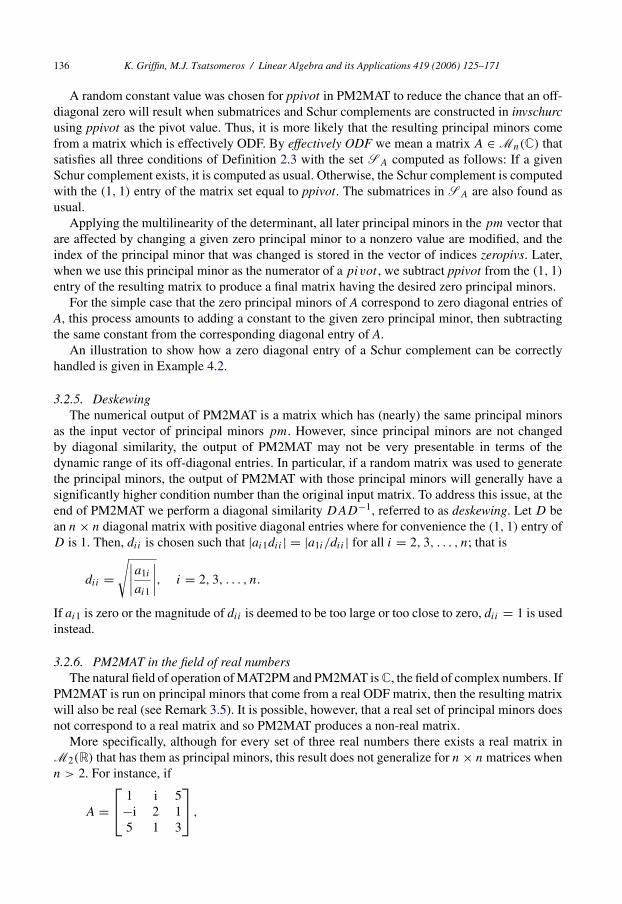
More specifically, although for every set of three real numbers there exists a real matrix inM2(R) that has them as principal minors, this result does not generalize for n × n matrices whenn > 2. For instance, if
A = 1 i 5
−i 2 15 1 3
,

K. Griffin, M.J. Tsatsomeros / Linear Algebra and its Applications 419 (2006) 125–171 137
then A is ODF and the principal minors of A in binary order are
pm = [1, 2, 1, 3, −22, 5, −48],which are certainly real. From the argument of Case n = 3 of Corollary 3.2, any matrix which hasthe same principal minors as A must be diagonally similar (with transpose) to A. Transpositiondoes not affect the field that A resides in. Without loss of generality consider a diagonal similarityof A by a diagonal matrix D with d11 = 1. Then
DAD−1 =1 0 0
0 d22 00 0 d33
1 i 5−i 2 15 1 3
1 0 0
0 1d22
0
0 0 1d33
=
1 i
d22
5d33
−id22 2 d22d33
5d33d33d22
3
is non-real for all d22, d33 ∈ C. That is, pm ∈ R7 above can only correspond to a non-real matrixand such will be the output of PM2MAT.
3.3. Operation count
The approximate number of floating point operations required by PM2MAT can be found bycounting the operations required to perform the following two primary inner loop tasks:
(a) solving the quadratics (3.7) in solveright and(b) evaluating equations of the form (3.9) to select the appropriate quadratic solution.
Task (a)Solving (3.7) is done once for every entry in the upper triangular part of every matrix in
level n − 2 through level 0. So, for an m × m matrix, there will be m(m − 1)/2 quadratics solved.Letting q be the number of floating point operations to solve the quadratic (which is approximately40), the total number of floating point operations in PM2MAT solving quadratics is
n−3∑k=0
2k(n − (k + 1))(n − (k + 2))q/2 = q · 2n − (q/2)(n2 + n + 2), (3.11)
which is of O(2n).Task (b)Let p be the number of floating point operations to evaluate Eq. (3.9) (which is approximately
11). For a given m × m matrix, m � 3, there are eight evaluations of (3.9) for the lower right3 × 3 submatrix (to choose the correct r(1), s(1), t (1) of (3.10)), 4(m − 3) evaluations (to finds(2), t (2), s(4), t (4) of (3.10)) and 2(m − 2)(m − 3)/2 = (m − 2)(m − 3) evaluations to find theremaining parameters below the second subdiagonal of each matrix (parameters t (3), t (5), t (6) of(3.10)). Thus, the total number of operations needed for these computations is
p
n−4∑k=0
2k(8 + 4(n − (k + 4)) + (n − (k + 3))(n − (k + 4))) = p(2 · 2n − (n2 + n + 4)).
(3.12)
Since this is also of O(2n), the total operation count is O(2n). Other incidental computations(various mins, building the (m + 1) × (m + 1) matrix at the end of invschurc, etc.) have no effecton the order of the computation and do not significantly add to the total number of operations.

138 K. Griffin, M.J. Tsatsomeros / Linear Algebra and its Applications 419 (2006) 125–171
3.4. Strategy for solving PMAP via PM2MAT and MAT2PM
First, we illustrate that if A ∈ Mn(C) is not ODF, then the principal minors of A may not beinvertible by PM2MAT into a matrix. We consider examples that violate each part of Definition 2.3.
Case (a): An off-diagonal entry of a matrix in SA is zeroSuppose we use PM2MAT to find a matrix with the principal minors of
A =−4 −3 −8
2 3 58 6 7
.
Since the (2, 1) entry of A/A[1] is zero, we could run into difficulties. Running the MAT2PMalgorithm on this matrix we obtain:
A =−4 −3 −8
2 3 58 6 7
, (Level 0)
LA =[
3 56 7
], RA =
[32 10 −9
], (Level 1)
Running PM2MAT on the principal minors of A, we see that PM2MAT is able to producematrices diagonally similar to LA and RA at its level 1.
LB =[
3 103 7
], RB =
[32 10 −9
], (Level 1)
Unfortunately, the zero in the (2, 1) entry of RB causes a divide by zero in Eq. (3.7). Therefore,PM2MAT is unable to find the diagonal similarity that makes rank(LB − RB) = 1, and PM2MATwill not produce an output matrix with the desired principal minors. Although it is possibleto add heuristics to PM2MAT to deal with this particular example, in general, the algebraicmethods employed in invschurc (see particularly (3.7) and (3.9) in Section 3.2.3) break downwhen off-diagonal zeros occur in any of the matrices generated by PM2MAT.
Case (b): Rank condition for partitions of 〈m〉 not satisfied for matrices in SAConsider the first two levels of the MAT2PM algorithm with the following input matrix A:
A =
2 −3 7 1 14 5 −3 1 14 −4 13 1 11 1 1 8 21 1 1 7 5
, (Level 0)
LA =
5 −3 1 1
−4 13 1 11 1 8 21 1 7 5
, RA =
11 −17 −1 −12 −1 −1 −152 − 5
2152
32
52 − 5
2132
92
. (Level 1)
Note that
rank(LA[{1, 2}, {3, 4}]) = rank(LA[{3, 4}, {1, 2}]) = 1,
rank(RA[{1, 2}, {3, 4}]) = rank(RA[{3, 4}, {1, 2}]) = 1,
where α = {1, 2} and β = {3, 4} form a partition of 〈4〉.

K. Griffin, M.J. Tsatsomeros / Linear Algebra and its Applications 419 (2006) 125–171 139
When PM2MAT is run with the principal minors of A as input, we produce the followingmatrices for level 1:
LB =
5 12
5 − 465 − 1
65
5 13 113
152
− 654 13 8 7
4
−65 52 8 5
, RB =
11 − 34
11 − 511 − 13
33
11 −1 − 52 − 13
6112 −1 15
21310
16526 − 15
13152
92
. (Level 1)
One may verify that LA and LB have the same principal minors. Likewise, RA and RB havethe same principal minors. However, since the conditions of Theorem 3.1 are not satisfied for LA,LB need not be diagonally similar with transpose to LA, and indeed this is the case. When solvingthe 3 sets of quadratics to make the lower right 3 × 3 submatrix of LB − RB rank 1, there aretwo combinations of solutions that both make rank(LB(1) − RB(1)) = 1. By chance, the wrongsolution is chosen, so the computation fails for the matrices as a whole. Solving the quadratics ofEq. (3.7) for the rest of the entries of the matrices does not yield a combination of solutions thatmakes rank(LB − RB) = 1.
By coincidence, RA and RB are diagonally similar with transpose, but the L matrices not beingdiagonally similar with transpose is sufficient to cause the computations of invschurc to fail.
Although this example suggests that (c) may imply (b) under the condition of (a) of Definition2.3, the converse is certainly not true as the following example shows.
Case (c): There exist multiple solutions which make rank(L − R)= 1Similar to the last case, the operation of MAT2PM on A ∈ M4(R) is summarized below down
to level 2.
A =
3 −6 −9 121 3 −7 − 4
3
2 2 −1 − 169
3 1 1 4
, (Level 0)
LA =3 −7 − 4
3
2 −1 − 169
1 1 4
, RA =5 −4 − 16
3
6 5 − 889
7 10 −8
, (Level 1)
[−1 − 16
9
1 4
],
[5 − 88
9
10 −8
],
[113 − 8
9103
409
],
[495 − 152
45785 − 8
15
]. (Level 2)
Running PM2MAT on the principal minors of A above yields:[−1 16
9
−1 4
],
[5 − 176
9
5 −8
],
[113 − 80
99113
409
],
[495 − 3952
735495 − 8
15
], (Level 2)
LB = 3 − 14
389
3 −1 169
− 32 −1 4
, RB = 5 − 14
5 − 11215
607 5 − 176
9
5 5 −8
, (Level 1)

140 K. Griffin, M.J. Tsatsomeros / Linear Algebra and its Applications 419 (2006) 125–171
B =
3 9
292 12
− 43 3 − 14
389
−4 3 −1 169
3 − 32 −1 4
. (Level 0)
Although LA is diagonally similar to LB and RA is diagonally similar to RB , there are twosolutions that make rank(LB − RB) = 1. Instead of choosing the dot similarity with RB
R1 = 5 − 8
3329
9 5 889
− 212 −10 −8
which has determinant 712/3 like RA and RB , the dot similarity
R2 = 5 − 8
3569
9 5 1609
−6 − 112 −8
with determinant 260 is chosen, which also satisfies rank(LB − R2) = 1. Therefore, the resultingB which is computed with R2 above is not diagonally similar to A. In fact, B is diagonally similarto
C =
3 −3 −9/2 12
2 3 −7 −4/3
4 2 −1 −16/93 1 1 4
,
where only the boxed entries differ from A. The principal minors of C (and B) are the same as theprincipal minors of A with the exception of the determinant. Note that the output of PM2MAT inthis example is dependent on small round-off errors which may vary from platform to platform.
Although it would be easy to add code to PM2MAT to resolve this ambiguity for the case thatL, R ∈ M3(C), in general, the method of invschurc which finds solutions for making rank(L −R) = 1 by working from the trailing 3 × 3 submatrix of L and R and progressing towards theupper right (see Eq. (3.10)) is not well suited to also preserving diagonal similarity with transposein cases where (c) of Definition 2.3 is not satisfied.
If the input principal minors do come from a matrix which is ODF, then PM2MAT will succeedin building a matrix that has them as principal minors up to numerical limitations. The followingproposition states this formally:
Proposition 3.7. Let pm ∈ C2n−1, n ∈ N be given. Suppose A ∈ Mn(C) is ODF. IfMAT2PM(A) = pm and B = PM2MAT(pm), then MAT2PM(B) = pm.
Proof. Let C ∈ Mm(C), m � 2 be any submatrix or Schur complement produced by runningMAT2PM on A (C ∈ SA). Since A is ODF, C has no off-diagonal zero entries and thus
L − R = C(1) − C/C[1] = C(1, 1]C[1, 1)/C[1]has no zero entries. Hence, rank(L − R) /= 0 for all such C.

K. Griffin, M.J. Tsatsomeros / Linear Algebra and its Applications 419 (2006) 125–171 141
Level n − 1 can always be created which matches the output of level n − 1 of MAT2PM(A)exactly, since this level of 1 × 1 matrices just consists of ratios of principal minors, where zeroprincipal minors can be handled using the multilinearity of the determinant (see Section 3.2.4).
For all the 2 × 2 matrices of level n − 2, rank(L − R) /= 0 for each matrix we produce, so weare able to compute matrices which have the same principal minors as each of the corresponding2 × 2 matrices of level n − 2 we get from running MAT2PM on A. By Corollary 3.3, the matricesproduced by PM2MAT are diagonally similar with transpose to the ones produced by MAT2PM,so by solving equations of the form of (3.7) (which always have solutions since if A is ODF,division by zero never occurs) we can modify R so rank(L − R) = 1 for each matrix of this level.
For subsequent levels, conditions (a) and (b) of Definition 2.3 guarantee that a diagonal sim-ilarity with transpose for all the R matrices exists so that rank(L − R) = 1 for each L, R pair.Furthermore, condition (c) of the same definition guarantees that the dot similarity found byinvschurc is sufficient to find this (unique, if L is regarded as fixed) similarity.
Proceeding inductively we see that the final matrixB output by PM2MAT has the same principalminors as A, since B has the same (1,1) entry as A, L = B(1) is diagonally similar with transposeto A(1) and R = B/B[1] is diagonally similar with transpose to A/A[1]. The MAT2PM algorithmcan then be used to verify that B and A have identical corresponding principal minors. �
Note that identical reasoning extends the result above to effectively ODF matrices.If the input principal minors do not come from an effectively ODF matrix, PM2MAT may fail to
produce a matrix with the desired principal minors. If the input principal minors are inconsistent,that is, a matrix which has them as principal minors does not exist, PM2MAT will always fail toproduce a matrix with the input principal minors.
When PM2MAT fails due to either inconsistent principal minors or due to principal minorsfrom an non-ODF matrix, it produces a matrix which does not have all the desired principalminors; no warning that this has occurred is guaranteed, since the warnings in PM2MAT dependupon numerical thresholds.
This suggests the following strategy for attempting to solve PMAP with principal minors froman unknown source with PM2MAT.
1. PM2MAT is run on the input principal minors and an output matrix A is produced.2. Then, MAT2PM is run on the matrix A, producing a second set of principal minors.3. These principal minors are compared to the original input principal minors. If they agree
to an acceptable tolerance, PM2MAT succeeded. Otherwise, the principal minors are eitherinconsistent or they are not realizable by a matrix which is effectively ODF.
A sample implementation of this strategy is provided in PMFRONT in Appendix B.
4. Illustrative examples
Example 4.1. We obtain a moderately scaled set of integer principal minors that correspond to areal matrix. To do this, we use MAT2PM to find the principal minors of
A =
−6 3 −9 4−6 −5 3 63 −3 6 −71 1 −1 −3
,

142 K. Griffin, M.J. Tsatsomeros / Linear Algebra and its Applications 419 (2006) 125–171
yielding
pm = 1 2 3 4 5 6 7
[1] [2] [1, 2] [3] [1, 3] [2, 3] [1, 2, 3]−6 −5 48 6 −9 −21 −36
8 9 10 11 12 13 14 15[4] [1, 4] [2, 4] [1, 2, 4] [3, 4] [1, 3, 4] [2, 3, 4] [1, 2, 3, 4]−3 14 9 −94 −25 96 59 6
.
For ease of reference, the first row of the above displayed pm contains the index of a givenprincipal minor, the second row is the index set used to obtain the submatrix correspondingto that minor, while the third row contains the value of the principal minor itself. For conve-nience, the utility PMSHOW in Appendix G has been included, which produces output similarto this for any input set of principal minors. To actually call PM2MAT, pm is just the vec-tor of values in the third row. Thus we can easily see that pm13 = det(A[1, 3, 4]) = 96, forexample.
Since there are 24 − 1 entries in pm, we desire to find a matrix B ∈ M4(R) which has thevalues in pm as its principal minors. We begin with level = 3 and produce matrices equivalent inall principal minors at each level to the ones that would have been produced by running MAT2PMon A.
Level 3At level 3 we desire to find eight 1 × 1 matrices whose entries are just the pivots in binary
order. Since the principal minors are stored in binary order (see Definition 3.4 and [2, Proposition4.6]) we compute the following quotients of consecutive principal minors:
pm8 = det(A[4]) = −3,
pm9
pm1= det(A[1, 4])
det(A[1]) = −7
3, . . . ,
pm15
pm7= det(A[1, 2, 3, 4])
det(A[1, 2, 3]) = −1
6.
Therefore, the desired level 3 matrices are
[−3], [− 73
],
[− 9
5
],
[− 47
24
],
[− 25
6
],
[− 32
3
],
[− 59
21
],
[− 1
6
].
Level 2Analogously to the previous level, we can now compute the four pivots of the four 2 × 2
matrices from the eight matrices of the previous level:
pm4 = 6,pm5
pm1= 3
2,
pm6
pm2= 21
5,
pm7
pm3= −3
4.
Since the first four 1 × 1 matrices of the previous level are submatrices of the four matrices wedesire to compute, we know that these matrices have the form
B =[
6 ∗∗ −3
],
[ 32 ∗∗ − 7
3
],
[ 215 ∗∗ − 9
5
],
[− 34 ∗
∗ − 4724
],
where the ∗’s indicate entries not yet known. Consider producing the first of these matrices,labeled B and partitioned as follows:
B =[
B[1] B[1, 1)
B(1, 1] B(1)
].
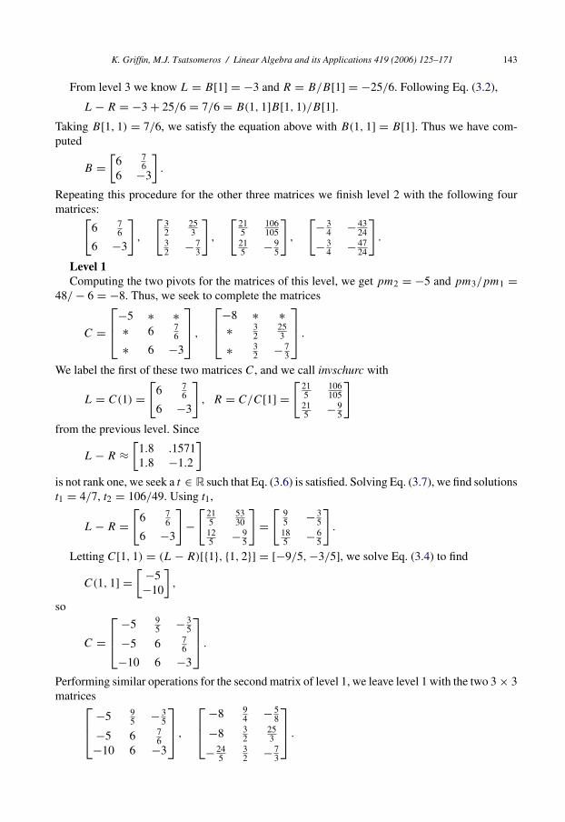
K. Griffin, M.J. Tsatsomeros / Linear Algebra and its Applications 419 (2006) 125–171 143
From level 3 we know L = B[1] = −3 and R = B/B[1] = −25/6. Following Eq. (3.2),
L − R = −3 + 25/6 = 7/6 = B(1, 1]B[1, 1)/B[1].Taking B[1, 1) = 7/6, we satisfy the equation above with B(1, 1] = B[1]. Thus we have com-puted
B =[
6 76
6 −3
].
Repeating this procedure for the other three matrices we finish level 2 with the following fourmatrices:[
6 76
6 −3
],
[32
253
32 − 7
3
],
[215
106105
215 − 9
5
],
[− 34 − 43
24
− 34 − 47
24
].
Level 1Computing the two pivots for the matrices of this level, we get pm2 = −5 and pm3/pm1 =
48/ − 6 = −8. Thus, we seek to complete the matrices
C =−5 ∗ ∗
∗ 6 76
∗ 6 −3
,
−8 ∗ ∗∗ 3
2253
∗ 32 − 7
3
.
We label the first of these two matrices C, and we call invschurc with
L = C(1) =[
6 76
6 −3
], R = C/C[1] =
[215
106105
215 − 9
5
]from the previous level. Since
L − R ≈[
1.8 .15711.8 −1.2
]is not rank one, we seek a t ∈ R such that Eq. (3.6) is satisfied. Solving Eq. (3.7), we find solutionst1 = 4/7, t2 = 106/49. Using t1,
L − R =[
6 76
6 −3
]−
[215
5330
125 − 9
5
]=
[95 − 3
5185 − 6
5
].
Letting C[1, 1) = (L − R)[{1}, {1, 2}] = [−9/5, −3/5], we solve Eq. (3.4) to find
C(1, 1] =[ −5−10
],
so
C = −5 9
5 − 35
−5 6 76
−10 6 −3
.
Performing similar operations for the second matrix of level 1, we leave level 1 with the two 3 × 3matrices −5 9
5 − 35
−5 6 76−10 6 −3
,
−8 94 − 5
8
−8 32
253
− 245
32 − 7
3
.

144 K. Griffin, M.J. Tsatsomeros / Linear Algebra and its Applications 419 (2006) 125–171
Level 0Given pivot = B[1] = pm1 = −6 and
L = B(1) = −5 9
5 − 35
−5 6 76
−10 6 −3
, R = B/B[1] = −8 9
4 − 58
−8 32
253
− 245
32 − 7
3
,
we desire to find the 4 × 4 matrix B of the form
B =
−6 ∗ ∗ ∗∗ −5 9
5 − 35
∗ −5 6 76
∗ −10 6 −3
.
As in the previous level, rank(L − R) /= 1, so we find r , s, t , such that Eq. (3.8) is satisfied.Solving Eq. (3.7) for each 2 × 2 submatrix of L − R, we obtain two quadratic solutions for r , s
and t :
r1 = 20/7, r2 = 10, s1 = 5/2, s2 = 5/16, t1 = 25/36, t2 = 25/8.
Then, comparing Eq. (3.9) for each of the 8 possible combinations, we find that only r = r2,s = s2, t = t2 makes rank(L − R) = 1. Applying this r , s, and t to R we obtain a R̂ which is dotsimilar to R:
R̂ = −8 9
4s− 5
8t
−8s 32
253r
− 24t5
3r2 − 7
3
= −8 36
5 − 15
− 52
32
56
−15 15 − 73
.
In this case, R̂ = DRD−1 with
D =1 0 0
0 516 0
0 0 258
,
and no transpose is necessary.Now,
L − R̂ = −5 9
5 − 35
−5 6 76
−10 6 −3
− −8 36
5 − 15
− 52
32
56
−15 15 − 73
= 3 − 27
5 − 25
− 52
92
13
5 −9 − 23
.
Since 9/2 of row 2 is the maximum absolute diagonal entry of L − R̂, we let B[1, 1) = (L −R̂)[2, {1, 2, 3}] = [−5/2, 9/2, 1/3] and by Eq. (3.4) we find
B(1, 1] = 36
5
−612
,
so
B =
−6 − 5
292
13
365 −5 9
5 − 35
−6 −5 6 76
12 −10 6 −3
.

K. Griffin, M.J. Tsatsomeros / Linear Algebra and its Applications 419 (2006) 125–171 145
Of course B is not equal to the original matrix A, but A = DBD−1 where
D =
1 0 0 00 − 5
6 0 00 0 − 1
2 00 0 0 1
12
.
For simplicity of illustration, the deskewing of Section 3.2.5 has not been applied to the outputmatrix B.
Example 4.2. To show how zero principal minors are handled as discussed in Section 3.2.4, weconsider running PM2MAT on the principal minors of the effectively ODF matrix
A =2 2 5
2 2 −37 3 −1
.
Using the convention of Example 4.1, A has principal minors:
pm = 1 2 3 4 5 6 7
[1] [2] [1, 2] [3] [1, 3] [2, 3] [1, 2, 3]2 2 0 −1 −37 7 −64
.
The 1 × 1 matrices of level 2 consist of the ratios
[pm4], [pm5/pm1], [pm6/pm2], [pm7/pm3]. (Level 2)
Since pm3 = 0, building these matrices would fail if the zero principal minor code were notinvoked.
The goal of zero principal minor loop at the beginning of PM2MAT is to create a consistent(taking into account the modified pivot entries) set of principal minors where the initial 2n−1 − 1principal minors are nonzero. It does this by making all the pivot or (1,1) entries of the matricesthat correspond to zero principal minors have pivots equal to ppivot instead of zero.
In the example at hand, we will take ppivot = 1 for simplicity. Since pm3 is computedby knowing that the pivot entry of the right matrix of level 1 is pm3/pm1, we assign pm3 =ppivot · pm1 = 1 · 2 = 2. Of course, in general, changing a single principal minor does not evenresult in a set of principal minors that are consistent, so the next part of the zero principal minor loopis devoted to computing the sums of principal minors that follow from applying the multilinearityof the determinant (also see the discussion of zero pivots in [2]) to the change just made. Sincepm3 is found from the (1,1) entry of A/A[1], only principal minors from descendants (in the topto bottom sense of the tree of Fig. 1) of the Schur complement of A/A[1] need to change. Theonly principal minor that satisfies this condition is pm7. Thus, the remaining required change tothe vector of principal minors is to let pm7 = pm7 + ppivot · pm5 = −64 + (−37) = −101.The final set of principal minors that we enter the main loop of PM2MAT is then
nzpm = 1 2 3 4 5 6 7
[1] [2] [1, 2] [3] [1, 3] [2, 3] [1, 2, 3]2 2 2 −1 −37 7 −101
,
where nzpm signifies “nonzero principal minors”. The first two levels of PM2MAT then yield
[−1], [−37/2], [7/2], [−101/2], (Level 2)
L =[
2 − 92
2 −1
], nzR =
[ppivot = 1 32
1 − 372
]. (Level 1)
146 K. Griffin, M.J. Tsatsomeros / Linear Algebra and its Applications 419 (2006) 125–171
At this point we recall that nzpm was designed to create ppivot = 1 in the (1, 1) entry of thematrix nzR, but the original principal minors corresponded to the (1, 1) entry of nzR being zero.Subtracting ppivot = 1 from nzR[1] and continuing we obtain:
L =[
2 − 92
2 −1
], R =
[0 32
1 − 372
], (Level 1)
B = 2 − 10
3352
− 65 2 − 9
2
2 2 −1
. (Level 0)
Note that B is diagonally similar to A with transpose, and thus has the principal minors pm. Ifwe had continued to run PM2MAT with the level 1 matrix nzR, we would have obtained a matrixthat had the principal minors nzpm instead.
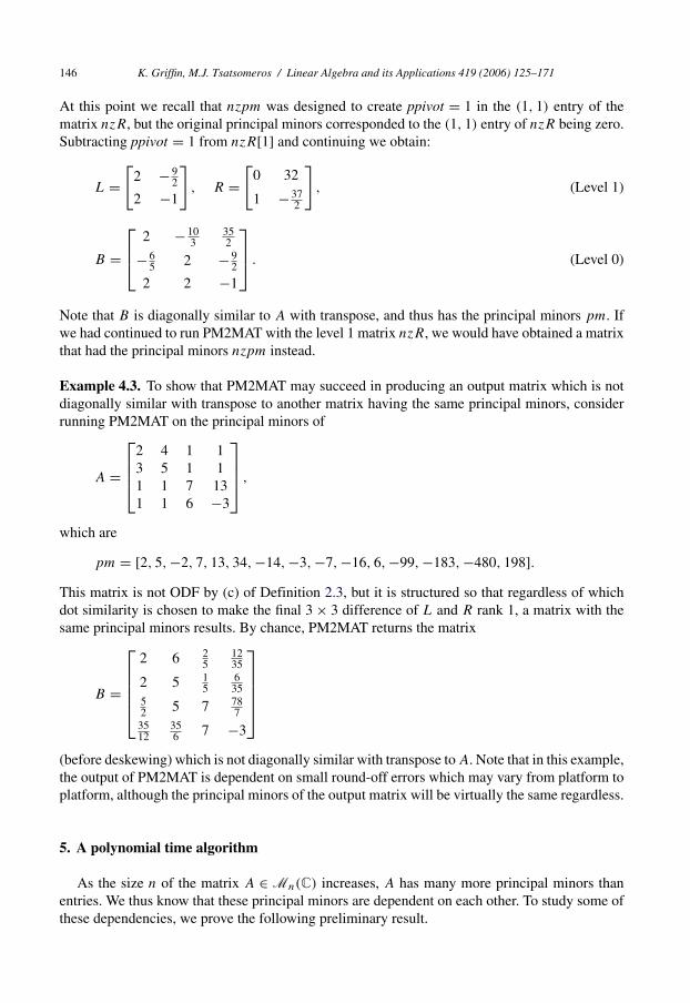
Example 4.3. To show that PM2MAT may succeed in producing an output matrix which is notdiagonally similar with transpose to another matrix having the same principal minors, considerrunning PM2MAT on the principal minors of
A =
2 4 1 13 5 1 11 1 7 131 1 6 −3
,
which are
pm = [2, 5, −2, 7, 13, 34, −14, −3, −7, −16, 6, −99, −183, −480, 198].This matrix is not ODF by (c) of Definition 2.3, but it is structured so that regardless of whichdot similarity is chosen to make the final 3 × 3 difference of L and R rank 1, a matrix with thesame principal minors results. By chance, PM2MAT returns the matrix
B =
2 6 2
51235
2 5 15
635
52 5 7 78
73512
356 7 −3
(before deskewing) which is not diagonally similar with transpose to A. Note that in this example,the output of PM2MAT is dependent on small round-off errors which may vary from platform toplatform, although the principal minors of the output matrix will be virtually the same regardless.
5. A polynomial time algorithm
As the size n of the matrix A ∈ Mn(C) increases, A has many more principal minors thanentries. We thus know that these principal minors are dependent on each other. To study some ofthese dependencies, we prove the following preliminary result.

K. Griffin, M.J. Tsatsomeros / Linear Algebra and its Applications 419 (2006) 125–171 147
Lemma 5.1. Let A ∈ Mn(C), n � 4, have 2n − 1 principal minors {pm1, pm2, . . . , pm2n−1}.If A is ODF, then pm2n−1 is determined by {pm1, pm2, . . . , pm2n−2}.
Proof. Let {pm1, pm2, . . . , pm2n−2, ˆpm2n−1} be passed to PM2MAT where ˆpm2n−1 /= pm2n−1and for convenience ˆpm2n−1 /= 0. The proof proceeds by showing that the 4 × 4 matrices of leveln − 4 using this set of principal minors with the last principal minor modified will be identical tothose 4 × 4 matrices of level n − 4 we would have obtained using the original principal minors{pm1, pm2, . . . , pm2n−2, pm2n−1}.
The queue of 1 × 1 matrices of level n − 1 will be identical to the queue of 1 × 1 matricesof level n − 1 using the original principal minors {pm1, pm2, . . . , pm2n−2, pm2n−1} except forthe last value. Therefore, the queue of 2 × 2 matrices of level n − 2 will be identical to the samequeue using the original principal minors except for the final matrix, whose (1,2) entry will bedifferent. Let
R =[r11 ˆr12r21 r22
]be the last matrix of level n − 2. Let B be the last matrix of level n − 3 we desire to produce fromlevel n − 2 and as usual we have R = B/B[1] and L = B(1). When we solve the quadratic Eq.(3.7) and modify R so that rank(L − R) = 1, we have
C = L − R =[c11 ˆc12ˆc21 c22
],
where only ˆc12 and ˆc21 are different from entries we would have obtained using the originalprincipal minors. Note, however, that rank(L − R) = rank(C) = 1 implies that det(C) = 0, soin fact ˆc12 ˆc21 = c12c21. Hence, C is diagonally similar to the matrix we would have obtained usingthe original principal minors. Although B will be different from the B we would have obtainedwith the original principal minors, it will only be different in its (1,3) and (3,1) entries (or (1,2)and (2,1) entries, depending on the relative magnitudes of c11 and c22 by Eqs. (3.3), (3.4) and(3.5)), while the product of these entries will be the same. Since A is ODF and B is dot similarto the corresponding Schur complement of A, there will only be one dot similarity with B thatwill make the difference of B with its corresponding left matrix rank 1 (see (c) of Definition 2.3).Therefore, all the 4 × 4 matrices of level n − 4 will be identical to those that were obtained usingthe original principal minors. �
Example 5.2. To illustrate the above lemma, let us revisit Example 4.1 from Section 4. Theoperation of PM2MAT is summarized as follows:
pm = [−6, −5, 48, 6, −9, −21, −36, −3, 14, 9, −94, −25, 96, 59, 6]
[−3], [− 73
],
[− 9
5
],
[− 47
24
],
[− 25
6
],
[− 32
3
],
[− 59
21
],
[− 1
6
](Level 3)[
6 76
6 −3
],
[32
253
32 − 7
3
],
[215
106105
215 − 9
5
],
[− 34 − 43
24
− 34 − 47
24
](Level 2)
−5 95 − 3
5
−5 6 76
−10 6 −3
,
−8 94
152
−8 32
253
25
32 − 7
3
(Level 1)

148 K. Griffin, M.J. Tsatsomeros / Linear Algebra and its Applications 419 (2006) 125–171−6 − 5
292
13
365 −5 9
5 − 35
−6 −5 6 76
12 −10 6 −3
(Level 0)
If instead we use the input (entries that are different are in bold)
pm = [−6, −5, 48, 6, −9, −21, −36, −3, 14, 9, −94, −25, 96, 59, 1]we obtain
[−3], [− 73
],
[− 9
5
],
[− 47
24
],
[− 25
6
],
[− 32
3
],
[− 59
21
],
[− 1
36
](Level 3)
[6 7
6
6 −3
],
[32
253
32 − 7
3
],
[215
106105
215 − 9
5
],
[− 34 − 139
72
− 34 − 47
24
](Level 2)
−5 95 − 3
5
−5 6 76
−10 6 −3
,
−8 94 −0.6304 . . .
−8 32
253
−4.7590 . . . 32 − 7
3
(Level 1)
−6 − 5
292
13
365 −5 9
5 − 35
−6 −5 6 76
12 −10 6 −3
(Level 0)
Rational expressions for the (1, 3) and (3, 1) entries of the last matrix of level 1 do not exist, butnote that (15/2) · (2/5) = 3 ≈ (−0.6304) · (−4.7590).
As a consequence to Lemma 5.1 we observe that generically all the “large” principal minorsof a matrix can be expressed in terms of the “small” principal minors.
Theorem 5.3. Let A ∈ Mn(C), n � 4. If A is ODF, each principal minor which is indexed by aset with 4 or more elements can be expressed in terms of the principal minors which are indexedby 3 or fewer elements.
Proof. Consider all the submatrices of A indexed by exactly 4 elements. Applying Lemma 5.1 toeach of them, we see that all of the principal minors indexed by exactly 4 elements are functionsof all the smaller principal minors (the determinants of all 1 × 1, 2 × 2 and 3 × 3 principalsubmatrices of A). Applying Lemma 5.1 to each principal minor of A indexed by exactly 5elements, these are functions of all of the principal minors indexed by 4 or fewer elements.However, all the principal minors with exactly 4 elements are functions of the principal minorsindexed by 3 or fewer elements, so all the principal minors indexed by 5 elements are functionsof the principal minors indexed by 3 or fewer elements. The result follows by induction. �

K. Griffin, M.J. Tsatsomeros / Linear Algebra and its Applications 419 (2006) 125–171 149
Theorem 5.3 motivates a “fast” version of PM2MAT that only takes as inputs the 1 × 1,2 × 2 and 3 × 3 principal minors but produces the same output matrix as PM2MAT if the inputprincipal minors come from a ODF matrix. To this end, a matching, fast (polynomial time)version of MAT2PM was written to produce only these small principal minors and is describedfirst.
FMAT2PMor a ODF matrix of size n, there are only
(n
1
)+
(n
2
)+
(n
3
)= n + n(n − 1)
2+ n(n − 1)(n − 2)
6= n(n2 + 5)
6
principal minors with index sets of size � 3 on which all the other principal minors depend. A fastand limited version of MAT2PM was implemented that produces only these principal minors inthe function FMAT2PM in Appendix C. Instead of having 2k matrices at each level which yield2k principal minors at level = k, there are only(
k
2
)+
(k
1
)+
(k
0
)= k(k + 1)
2+ 1 (5.13)
matrices that need be computed resulting in the corresponding number of principal minors beingproduced. This is because at level = k we only need to compute those principal minors involv-ing the index k + 1 and 2 smaller indices to produce the principal minors which come from3 × 3 submatrices. The other two terms of (5.13) are similarly derived: the k + 1 index and1 smaller index is used to compute the principal minors which come from 2 × 2 submatrices,and each level has one new minor from the 1 × 1 submatrix which is referenced by the indexk + 1.
From (5.13), it is easily verified that at each level = k, precisely k more matrices are producedthan were computed at level = k − 1.
Simple logic can be used to determine which matrices in the input queue need to be processedto produce matrices in the output queue. If the (1,1) entry of a matrix corresponds to a principalminor with an index set of 2 or less (a 2 × 2 or 1 × 1 principal minor) then we take the submatrixand Schur complement of the matrix, just as we do in MAT2PM since this matrix will havedescendants which correspond to principal minors from 3 × 3 submatrices. However, if the (1, 1)
entry of a matrix corresponds to a principal minor with an index set of 3, then we only take thesubmatrix of this matrix; no Schur complement is computed or stored. This scheme preventsmatrices that would be used to find principal minors with an index set of 4 or more from everbeing computed. To keep track the index sets of the principal minors, the index of the principalminor as it would have been computed in MAT2PM is stored in the vector of indices pmidx. Inthe code, the MAT2PM indices in pmidx are referred to as the long indices of a principal minor,while the indices in the pm vector produced by FMAT2PM are called the short indices of a givenprincipal minor. The vector of long indices pmidx is output along with the vector of principalminors in pm by FMAT2PM.
At each level, the indices pertaining to the principal minors which are computed at that levelare put in pmidx. The following table shows how pmidx is incrementally computed at eachlevel:

150 K. Griffin, M.J. Tsatsomeros / Linear Algebra and its Applications 419 (2006) 125–171
level pmidx
0 [1, 0, 0, . . . , 0]1 [1, 2, 3, 0, 0, . . . , 0]2 [1, 2, 3, 4, 5, 6, 7, 0, . . . , 0]3 [1, 2, 3, 4, 5, 6, 7, 8, 9, 10, 11, 12, 13, 14, 0, . . . , 0]4 [1, 2, 3, 4, 5, 6, 7, 8, 9, 10, 11, 12, 13, 14, 16, 17,
18, 19, 20, 21, 22, 24, 25, 26, 28, 0, . . . , 0]...
...
As an aid to interpreting the values in pmidx, the utilities IDX2V and V2IDX in Appendix F andAppendix E respectively have been included. IDX2V takes a long index in pmidx and producesthe index set of the submatrix that corresponds to it and returns this as a vector. V2IDX is theinverse of this operation.
We note that FMAT2PM could be adapted analogously to compute all principal minors up toany fixed size of index set.
FPM2MATGiven pm and pmidx in the format produced by FMAT2PM, FPM2MAT can invert only these
1 × 1, 2 × 2 and 3 × 3 principal minors into a matrix that is unique up to diagonal similarity withtranspose if the principal minors come from a matrix which is ODF as a consequence of Theorem5.3.
It is not strictly necessary that pmidx be an input to FPM2MAT since it is fixed for anygiven matrix size n, but since pmidx is produced naturally by FMAT2PM and since pmidx canbe thought of with pm as implementing a very sparse vector format, pm and pmidx are inputtogether to FPM2MAT.
Since FPM2MAT processes levels from the largest (bottom) to smallest (top), it was usefulto make the vector ipmlevels at the beginning of FPM2MAT which contains the short indexof the beginning of each level. Then, at each level, FPM2MAT computes those matrices whichhave a submatrix (or left matrix L). If a Schur complement (an R matrix) exists for the matrixto be produced, this is input to invschurc just as in PM2MAT. Otherwise, a matrix of ones ispassed in for the Schur complement to invschurc, since the particular values will prove to be ofno consequence (see Example 5.2). Although this is slightly slower than just embedding L in alarger matrix, it has been found to produce more accurate results for large n.
The bulk of the operations of FPM2MAT including the subroutines invschurc, solveright anddeskew are unchanged from PM2MAT.
5.1. Notes on the operation of the fast versions
• FMAT2PM processes a 53 × 53 matrix in about the same time that MAT2PM can process a20 × 20 matrix.
• FPM2MAT can invert the 24857 “small” principal minors of a 53 × 53 real or complex matrixinto a matrix in M53 in a few minutes.
• Zero principal minors are not presently handled by either FMAT2PM or FPM2MAT for clarityof presentation, but the multilinearity of the determinant could be exploited in these programsto handle zero principal minors as is implemented in MAT2PM and PM2MAT.
• For FMAT2PM, only k + 1 matrices need to have Schur complements taken at each level = k.Thus, FMAT2PM is of order O(n4) since

K. Griffin, M.J. Tsatsomeros / Linear Algebra and its Applications 419 (2006) 125–171 151
n−2∑k=0
(k + 1)2(n − (k + 1))2 = 1
6(n4 − n2),
where there are generally 2 operations for each element of the Schur complement. The scalingof the outer product by the inverse of the appropriate principal minor only affects (n − (k + 1))
elements at level k.• It has been found that for numerical reasons it is desirable to call invschurc with a dummy
matrix of ones whenever the R Schur complement matrix is missing.• To find the approximate operation count for FPM2MAT, we note that the quadratics (3.7) need
to be solved for each upper triangular entry of each of the k(k + 1)/2 + 1 matrices (see (5.13))at each level = k. As in (3.11) we let q be the number of operations to solve the quadraticequation to find
n−3∑k=0
(k(k + 1)/2 + 1)(n − (k + 1))(n − (k + 2))q/2
= q
120(n5 − 5n4 + 25n3 − 55n2 + 34n).
Similarly, letting p be the number of operations to evaluate equations of the form (3.9),
p
n−4∑k=0
(k(k + 1)/2 + 1)(8 + 4(n − (k + 4)) + (n − (k + 3))(n − (k + 4)))
= p
60(n5 + 5n4 + 45n3 − 295n2 + 974n − 1320),
as in the sum of (3.12). Thus, FPM2MAT is O(n5).
6. Some consequences and remarks
In this section we will touch upon some subjects and problems related to PMAP and PM2MATin the form of remarks.
Remark 6.1. With PM2MAT we can at least partially answer a question posed by Holtz andSchneider in [3, problem (4) pp. 265–266]. The authors pose PMAP as one step toward theinverse problem of finding a GKK matrix with prescribed principal minors.
Given a set of principal minors, we can indeed determine via PM2MAT whether or not there isan effectively ODF matrix A that has them as its principal minors. To accomplish this, we simplyrun PM2MAT on the given set of principal minors, producing a matrix A. Then, we run MAT2PMon this matrix to see if the matrix A has the desired principal minors. If the principal minorsare consistent and belong to an effectively ODF matrix, the principal minors will match, up tonumerical limitations. If the principal minors cannot be realized by a matrix or if the principalminors do not belong to an effectively ODF matrix, then the principal minors of A will not matchthe input principal minors. In the former case, the generalized Hadamard–Fischer inequalities andthe Gantmacher–Krein–Carlson theorem (see [3]) can be used to decide whether there is a GKKand effectively ODF matrix with the given principal minors.

152 K. Griffin, M.J. Tsatsomeros / Linear Algebra and its Applications 419 (2006) 125–171
Remark 6.2. In Stouffer [5], it is claimed that for A ∈ Mn(C) there are only n2 − n + 1 “inde-pendent” principal minors that all the other principal minors depend on, and as the first exampleof such a “complete” set the following set is offered:
S = {A[i] : i ∈ 〈n〉} ∪ {A[i, j ] : i <j ; i, j ∈ 〈n〉} ∪ {A[1, i, j ] : i <j ; i, j ∈ {2, 3, . . . , n}}.Indeed, S contains(
n
1
)+
(n
2
)+
(n − 1
2
)= n2 − n + 1
principal minors. However, these principal minors are not independent since equations [5, (5) and(6), p. 358] may not even have solutions if the principal minors are not consistent or come froma matrix which is not ODF. Moreover, even generically, S does not determine A up to diagonalsimilarity with transpose for n � 4 since, in general, the last two equations of [5, (6), p. 358]have two solutions for each aij , aji pair. The set S in [5], however, does generically determinethe other principal minors of A up to a finite set of possibilities.
Remark 6.3. The conditions of Definition 2.3 are difficult to verify from an input set of principalminors from an unknown source without actually running the PM2MAT algorithm on them. Inparticular, part (c) is difficult to verify even if a matrix that has the same principal minors as theinput principal minors happens to be known. However, usually PM2MAT will print a warning ifthe conditions of the definition are not satisfied, and the strategy of Section 3.4 can be employedto quickly verify if PM2MAT has performed the desired task.
Remark 6.4. Note that Theorem 5.3 does not imply that the principal minors indexed by 3 orfewer elements are completely free. There are additional constraints among the smaller principalminors. If one chooses a set of principal minors indexed by 3 or fewer elements at random anduses FPM2MAT to invert these into a matrix A, the matrix A will not in general have the sameprincipal minors indexed by 3 or fewer elements as the input principal minors.
Remark 6.5. If a random vector of principal minors is passed to PM2MAT, the resulting matrixwill have all the desired 1 × 1 and 2 × 2 principal minors, and some of the 3 × 3 principal minorswill be realized as well. However, none of the larger principal minors will be the same as thosethat were in the input random vector of principal minors.
7. Future work
Here we summarize some of our main goals for the future regarding PMAP and PM2MAT.
• Incorporate into PMAP and its solution algorithm structural and qualitative requirements of thematrix solutions. For example, we may want to seek solutions of special structure (e.g., positivedefinite, Hessenberg, Toeplitz) or having other special attributes (e.g., specified directed graph,entrywise nonnegativity).
• Expand the functionality of PM2MAT from effectively ODF matrices to a broader class ofmatrices.
• Identify applications of PMAP in theoretical and applied mathematics, and contribute to thesolution of relevant problems.

K. Griffin, M.J. Tsatsomeros / Linear Algebra and its Applications 419 (2006) 125–171 153
• Examine the potential consequences and usage of our algorithmic approach to the P-problem.This the problem of checking whether a given matrix is a P-matrix or not. Recall that a P-matrixis one all of whose principal minors are positive. The P-problem is known to be an NP-hardproblem [1].To be more specific, note all the principal minors that FMAT2PM computes being positiveprovides a polynomial time necessary condition for a matrix to be a P-matrix. If the positivityof the larger minors could be predicted from these 1 × 1, 2 × 2 and 3 × 3 principle minorsfor ODF matrices, then it would be possible to realize a polynomial time algorithm for theP-problem applied to this class of matrices.
Acknowledgments
The authors are grateful to an anonymous referee for a careful examination of the first draftof this paper leading to the introduction of condition (c) of Definition 2.3 and for several otherimprovements to the manuscript.
Appendix A. PM2MAT
% PM2MAT Finds a real or complex matrix that has PM as its principal% minors.%% PM2MAT produces a matrix with some, but perhaps not all, of its% principal minors in common with PM. If the principal minors are% not consistent or the matrix that has them is not ODF, PM2MAT will% produce a matrix with different principal minors without warning.% Run MAT2PM on the output matrix A as needed.%% A = PM2MAT(PM)% where PM is a 2^n - 1 vector of principal minors and A will be an n x n% matrix.%% The structure of PM, where |A[v]| is the principal minor of "A" indexed% by the vector v:% PM: |A[1]| |A[2]| |A[1 2]| |A[3]| |A[1 3]| |A[2 3]| |A[1 2 3]| ...function A = pm2mat(pm)myeps = 1e-10;n = log2(length(pm)+1);% Make first (smallest) entry of zeropivs an impossible indexzeropivs = 0;% Pick a random pseudo-pivot value that minimizes the chances that% pseudo-pivoting will create a non-ODF matrix.ppivot = 1.9501292851471754e+000;% initialize globals to allow warnings to be printed only onceglobal WARN_A WARN_C WARN_IWARN_A = false; WARN_C = false; WARN_I = false;

154 K. Griffin, M.J. Tsatsomeros / Linear Algebra and its Applications 419 (2006) 125–171
% To avoid division by zero, do an operation analogous to the zeropivot% loop in mat2pm.for i = 1:((length(pm)+1)/2 - 1)
if (abs(pm(i)) < myeps)mask = i;zeropivs = union(zeropivs, i);ipm1 = bitand(mask, bitcmp(msb(mask),48));if ipm1 == 0
pm(mask) = pm(mask) + ppivot;else
pm(mask) = (pm(mask)/pm(ipm1) + ppivot)*pm(ipm1);enddelta = msb(mask);delta2 = 2*delta;for j = mask+delta2:delta2:2^n - 1
pm(j) = pm(j) + ppivot*pm(j - delta);end
endendzeropivsidx = length(zeropivs) - 1;zeropivsmax = zeropivs(zeropivsidx+1);
% initial processing is special, no call to invschurc is necessarynq = 2^(n-1);q = zeros(1,1,nq);ipm1 = nq;ipm2 = 1;for i = 1:nq
if i == 1q(1,1,i) = pm(ipm1);
elseq(1,1,i) = pm(ipm1)/pm(ipm2);ipm2 = ipm2+1;
endipm1 = ipm1+1;
end
%% Main ’level’ loop%for level = n-2:-1:0 % for consistency with mat2pm levels
[n1, n1, nq] = size(q);nq = nq/2;n1 = n1+1;% The output queue has half the number of matrices, each one larger in% row and col dimension

K. Griffin, M.J. Tsatsomeros / Linear Algebra and its Applications 419 (2006) 125–171 155
qq = zeros(n1, n1, nq);ipm1 = 2*nq-1;ipm2 = nq-1;for i = nq:-1:1 % process matrices in reverse order for zeropivs
if (i == 1)pivot = pm(ipm1);
elsepivot = pm(ipm1)/pm(ipm2);ipm2 = ipm2-1;
endqq(:,:,i) = invschurc(pivot, q(:,:,i), q(:,:,i+nq));if zeropivsmax == ipm1
qq(1,1,i) = qq(1,1,i) - ppivot;zeropivsmax = zeropivs(zeropivsidx);zeropivsidx = zeropivsidx - 1;
endipm1 = ipm1-1;
endq = qq;
endA = q(:,:,1);A = deskew(A);
if WARN_A% ODF (a) not satisfiedfprintf(2,...
’PM2MAT: off diagonal zeros found, solution suspect.\n’);endif WARN_C
fprintf(2,...’PM2MAT: multiple solutions to make rank(L-R)=1, solution suspect.\n’);endif WARN_I
fprintf(2, ...’PM2MAT: input principal minors may be inconsistent, solution suspect.\n’);end
%% Suppose A is an (m+1) x (m+1) matrix such that%% pivot = A(1,1)% L = A(2:m+1, 2:m+1)% R = L - A(2:m+1,1)*A(1,2:m+1)/pivot = (the Schur’s complement with% respect to the pivot or A/A[1]).%% Then invschurc finds such an (m+1) x (m+1) matrix A (not necessarily

156 K. Griffin, M.J. Tsatsomeros / Linear Algebra and its Applications 419 (2006) 125–171
% unique) given the pivot (a scalar), and the m x m matrices L and R.%% If rank(L-R) is not 1, modifies R so that L-R is rank 1.%function A = invschurc(pivot, L, R)global WARN_C WARN_Imyeps_i = 1e-3*norm(R,inf); % make these relative to magnitude of Rmyeps_c = 1e-9*norm(R,inf);m = length(R);
% Try to make (L-R) rank 1if m == 2
[t1,t2] = solveright(L(1,1), L(1,2), L(2,1), L(2,2),...R(1,1), R(1,2), R(2,1), R(2,2));
% This is arbitrary, take the first.t = t1;
R(2,1) = R(2,1)*t;R(1,2) = R(1,2)/t;
elseif m >= 3% We start with the lower right hand 3x3 submatrix. We have 3% parameters, each with two possible solutions. Only 1 of the 8% possible solutions need give us a L-R which is rank 1. We find the% right solution by brute force.i1 = m-2;i2 = m-1;i3 = m;[r1,r2] = solveright(L(i2,i2), L(i2,i3), L(i3,i2), L(i3,i3),...
R(i2,i2), R(i2,i3), R(i3,i2), R(i3,i3));[s1,s2] = solveright(L(i1,i1), L(i1,i2), L(i2,i1), L(i2,i2),...
R(i1,i1), R(i1,i2), R(i2,i1), R(i2,i2));[t1,t2] = solveright(L(i1,i1), L(i1,i3), L(i3,i1), L(i3,i3),...
R(i1,i1), R(i1,i3), R(i3,i1), R(i3,i3));% Perform a parameterized "row reduction" on the first two rows of this% matrix and compute the absolute value of the (2,3) entry. One of% them will be nearly zero.r111 = abs((L(i2,i3) - R(i2,i3)/r1)*(L(i1,i1) - R(i1,i1)) - ...
(L(i2,i1) - R(i2,i1) * s1)*(L(i1,i3) - R(i1,i3)/t1));r112 = abs((L(i2,i3) - R(i2,i3)/r1)*(L(i1,i1) - R(i1,i1)) - ...
(L(i2,i1) - R(i2,i1)*s1)*(L(i1,i3) - R(i1,i3)/t2));r121 = abs((L(i2,i3) - R(i2,i3)/r1)*(L(i1,i1) - R(i1,i1)) - ...
(L(i2,i1) - R(i2,i1)*s2)*(L(i1,i3) - R(i1,i3)/t1));r122 = abs((L(i2,i3) - R(i2,i3)/r1)*(L(i1,i1) - R(i1,i1)) - ...
(L(i2,i1) - R(i2,i1)*s2)*(L(i1,i3) - R(i1,i3)/t2));r211 = abs((L(i2,i3) - R(i2,i3)/r2)*(L(i1,i1) - R(i1,i1)) - ...

K. Griffin, M.J. Tsatsomeros / Linear Algebra and its Applications 419 (2006) 125–171 157
(L(i2,i1) - R(i2,i1)*s1)*(L(i1,i3) - R(i1,i3)/t1));r212 = abs((L(i2,i3) - R(i2,i3)/r2)*(L(i1,i1) - R(i1,i1)) - ...
(L(i2,i1) - R(i2,i1)*s1)*(L(i1,i3) - R(i1,i3)/t2));r221 = abs((L(i2,i3) - R(i2,i3)/r2)*(L(i1,i1) - R(i1,i1)) - ...
(L(i2,i1) - R(i2,i1)*s2)*(L(i1,i3) - R(i1,i3)/t1));r222 = abs((L(i2,i3) - R(i2,i3)/r2)*(L(i1,i1) - R(i1,i1)) - ...
(L(i2,i1) - R(i2,i1)*s2)*(L(i1,i3) - R(i1,i3)/t2));rv = [r111, r112, r121, r122, r211, r212, r221, r222];mn = min(rv);if (r111 == mn)
r = r1; s = s1; t = t1;elseif (r112 == mn)
r = r1; s = s1; t = t2;elseif (r121 == mn)
r = r1; s = s2; t = t1;elseif (r122 == mn)
r = r1; s = s2; t = t2;elseif (r211 == mn)
r = r2; s = s1; t = t1;elseif (r212 == mn)
r = r2; s = s1; t = t2;elseif (r221 == mn)
r = r2; s = s2; t = t1;else % (r222 == mn)
r = r2; s = s2; t = t2;endif mn > myeps_i
WARN_I = true;endif sum(rv < myeps_c) > 1
WARN_C = true;endR(i3,i2) = R(i3,i2)*r;R(i2,i3) = R(i2,i3)/r;R(i2,i1) = R(i2,i1)*s;R(i1,i2) = R(i1,i2)/s;R(i3,i1) = R(i3,i1)*t;R(i1,i3) = R(i1,i3)/t;
% Now the lower right hand 3x3 submatrix of L-R has rank 1. Then we% fix up the rest of L-R.for i1 = m-3:-1:1
i2 = i1+1;i3 = i1+2;

158 K. Griffin, M.J. Tsatsomeros / Linear Algebra and its Applications 419 (2006) 125–171
% Now the inside lower right submatrix is done, so we% only have 2 free parameters and 4 combinations to examine.[s1,s2] = solveright(L(i1,i1), L(i1,i2), L(i2,i1), L(i2,i2),...
R(i1,i1), R(i1,i2), R(i2,i1), R(i2,i2));[t1,t2] = solveright(L(i1,i1), L(i1,i3), L(i3,i1), L(i3,i3),...
R(i1,i1), R(i1,i3), R(i3,i1), R(i3,i3));
r11 = abs((L(i2,i3) - R(i2,i3))*(L(i1,i1) - R(i1,i1)) - ...(L(i2,i1) - R(i2,i1)*s1)*(L(i1,i3) - R(i1,i3)/t1));
r12 = abs((L(i2,i3) - R(i2,i3))*(L(i1,i1) - R(i1,i1)) - ...(L(i2,i1) - R(i2,i1)*s1)*(L(i1,i3) - R(i1,i3)/t2));
r21 = abs((L(i2,i3) - R(i2,i3))*(L(i1,i1) - R(i1,i1)) - ...(L(i2,i1) - R(i2,i1)*s2)*(L(i1,i3) - R(i1,i3)/t1));
r22 = abs((L(i2,i3) - R(i2,i3))*(L(i1,i1) - R(i1,i1)) - ...(L(i2,i1) - R(i2,i1)*s2)*(L(i1,i3) - R(i1,i3)/t2));
rv = [r11, r12, r21, r22];mn = min(rv);if (r11 == mn)
s = s1; t = t1;elseif (r12 == mn)
s = s1; t = t2;elseif (r21 == mn)
s = s2; t = t1;else % (r22 == mn)
s = s2; t = t2;endif mn > myeps_i
WARN_I = true;endif sum(rv < myeps_c) > 1
WARN_C = true;endR(i2,i1) = R(i2,i1)*s;R(i1,i2) = R(i1,i2)/s;R(i3,i1) = R(i3,i1)*t;R(i1,i3) = R(i1,i3)/t;for j = i1+3:m
% Finally, once the second row of the submatrix we are working% on is uniquely solved, we just pick the solution to the% quadratic such that the first row is a multiple of the% second row. Note that one of r1, r2 will be almost zero.% Solving the quadratics leads to much better performance% numerically than just taking multiples of the second or% any other row.%

K. Griffin, M.J. Tsatsomeros / Linear Algebra and its Applications 419 (2006) 125–171 159
j1 = i1+1;[t1,t2] = solveright(L(i1,i1), L(i1,j), L(j,i1), L(j,j),...
R(i1,i1), R(i1,j), R(j,i1), R(j,j));r1 = abs((L(j1,j) - R(j1,j))*(L(i1,i1) - R(i1,i1)) - ...
(L(j1,i1) - R(j1,i1))*(L(i1,j) - R(i1,j)/t1));r2 = abs((L(j1,j) - R(j1,j))*(L(i1,i1) - R(i1,i1)) - ...
(L(j1,i1) - R(j1,i1))*(L(i1,j) - R(i1,j)/t2));if (r1 <= r2)
t = t1;else
t = t2;endrv = [r1, r2];if mn > myeps_i
WARN_I = true;endif sum(rv < myeps_c) > 1
WARN_C = true;end
R(j,i1) = R(j,i1)*t;R(i1,j) = R(i1,j)/t;
endend
end
B = (L-R); % a rank 1 matrix[mn, idxmax] = max(abs(diag(B)));% For numerical reasons use the largest diagonal element as a base to find% the two vectors whose outer product is B*pivotyT = B(idxmax,:);if yT(idxmax) == 0
% This shouldn’t happen normally, but to prevent% divide by zero when we set all "dependent" principal% minors (with index sets greater than or equal to a constant)% to the same value, let yT be something.yT = ones(1,m);
endx = B(:,idxmax)*pivot / yT(idxmax);A = zeros(m+1);A(1,1) = pivot;A(1,2:m+1) = yT;A(2:m+1,1) = x;A(2:m+1,2:m+1) = L;

160 K. Griffin, M.J. Tsatsomeros / Linear Algebra and its Applications 419 (2006) 125–171
%% Returns the two possible real solutions that will make L-R rank one if we% let% r21 = r21*t? (where ? = 1 or 2) and% r12 = r12/t?%function [t1,t2] = solveright(l11,l12,l21,l22,r11,r12,r21,r22)global WARN_Ax1 = l11-r11;x2 = l22-r22;d = sqrt(x1^2*x2^2 + l12^2*l21^2 + r12^2*r21^2 - 2*x1*x2*l12*l21 - ...
2*x1*x2*r12*r21-2*l12*l21*r21*r12);if (l12 == 0)||(r21 == 0)
% This shouldn’t happen normally, but to prevent% divide by zero when we set all "dependent" principal% minors (with index sets greater than or equal to a constant)% to the same value, let [t1,t2] be something.t1 = 1;t2 = 1;WARN_A = true;
elset1 = (-x1*x2 + l12*l21 + r12*r21 - d)/(2*l12*r21);t2 = (-x1*x2 + l12*l21 + r12*r21 + d)/(2*l12*r21);
% This also shouldn’t happen. Comment above applies.if (t1 == 0)||(t2 == 0)
WARN_A = true;if (t1 == 0)&&(t2 == 0)
t1 = 1;t2 = 1;
elseif (t1 == 0)% return better solution in t1 for m=2 case in invschurct1 = t2;t2 = 1;
else % (t2 == 0)t2 = 1;
endend
end
%% Makes abs(A(1,i)) = abs(A(i,1)) through diagonal similarity for all i.%function A = deskew(A)n = length(A);d = ones(n,1);

K. Griffin, M.J. Tsatsomeros / Linear Algebra and its Applications 419 (2006) 125–171 161
for i = 2:nif A(i,1) ~= 0 % don’t divide by 0
d(i) = sqrt(abs(A(1,i)/A(i,1)));if (d(i) > 1e6)||(d(i) < 1e-6)
% something is likely wrong, use 1 insteadd(i) = 1;
endend % else leave d(i) = 1
end
% If D = diag(d), this effectively computes A = D*A*inv(D)for i = 2:n
A(i,:) = A(i,:)*d(i);endfor i = 2:n
A(:,i) = A(:,i)/d(i);end
% Returns the numerical value of the most significant bit of x.% For example, msb(7) = 4, msb(6) = 4, msb(13) = 8.function m = msb(x)persistent MSBTABLE % MSBTABLE persists between calls to mat2pmif is empty(MSBTABLE)
% If table is empty, initialize itMSBTABLE = zeros(255,1);for i=1:255
MSBTABLE(i) = msbslow(i);end
end
m = 0;% process 8 bits at a time for speedif x ~= 0
while x ~= 0x1 = x;x = bitshift(x, -8); % 8 bit left shiftm = m + 8;
endm = bitshift(MSBTABLE(x1), m-8); % right shift
end
% Returns the numerical value of the most significant bit of x.% For example, msb(7) = 4, msb(6) = 4, msb(13) = 8. Slow version% used to build a table.function m = msbslow(x)m = 0;

162 K. Griffin, M.J. Tsatsomeros / Linear Algebra and its Applications 419 (2006) 125–171
if x ~= 0m = 1;while x ~= 0
x = bitshift(x, -1);m = 2*m;
endm = m/2;
end
Appendix B. PMFRONT
% PMFRONT Finds a real or complex matrix that has PM as its principal% minors if possible, prints out a warning if no such matrix can% be found by PM2MAT.%% A = PMFRONT(PM)% where PM is a 2^n - 1 vector of principal minors and A will be an n x n% matrix.%% The structure of PM, where |A[v]| is the principal minor of "A" indexed% by the vector v:% PM: |A[1]| |A[2]| |A[1 2]| |A[3]| |A[1 3]| |A[2 3]| |A[1 2 3]| ...function A = pmfront(pm)myeps = 1e-5; % tolerance for relative errors in the principal minors
% First run pm2matA = pm2mat(pm);
% Next, run mat2pm on the resultpm1 = mat2pm(A);
smallestpm = min(abs(pm));if smallestpm < 1e-10
fprintf(2, ...’There are principal minors very close to zero, relative errors in\n’);
fprintf(2, ...’principal minors may not be meaningful. Consider the absolute error\n’)
fprintf(2, ...’to decide if PM2MAT succeeded.\n’);
err = norm((pm-pm1),inf);
fprintf(2, ...’The maximum absolute error in the principal minors is %e\n’, err);else
% Compare the results in terms of the relative error in the pm’serr = norm((pm-pm1)./abs(pm),inf);

K. Griffin, M.J. Tsatsomeros / Linear Algebra and its Applications 419 (2006) 125–171 163
if err > myepsfprintf(2, ’PM2MAT failed\n’);fprintf(2, ...
’No matrix could be found that has all the requested principal minors.\n’);fprintf(2, ...
’The PM’’s are inconsistent or they come from a non-ODF matrix.\n’);else
fprintf(2, ’PM2MAT succeeded\n’);endfprintf(2, ...
’The maximum relative error in the principal minors is %e\n’, err);end
Appendix C. FMAT2PM
% FMAT2PM Finds all 1x1, 2x2 and 3x3 principal minors of an n x n matrix.% [PM, PMIDX] = FMAT2PM(A)% where "A" is an n x n matrix (zero pivots not handled).% MAT2PM returns a vector of all the 1x1, 2x2, and 3x3 principal minors% of the matrix "A" in PM. Also returns PMIDX, a vector of indices% that gives the index of the given principal minor in the full% binary ordered PM vector that MAT2PM produces. Thus, for example,% if%% A = rand(30);% [pm, pmidx] = fmat2pm(A);%% then%% det(A([25 29 30],[25 29 30]))%% is the same as%% pm(find(pmidx == v2idx([25 29 30])))function [pm, pmidx] = fmat2pm(a)% Only works on up to 53x53 matrices due to restrictions on indices.n = length(a);
% nchoosek(n,1) + nchoosek(n,2) + nchoosek(n,3);pm = zeros(1, (n^2 + 5)*n/6); % where the principal minors are storedpmidx = zeros(1, (n^2 + 5)*n/6); % place to store full (mat2pm) indicespmidx(1) = 1;ipm = 1; % short (new) index for storing principal minorsq = zeros(n,n,1); % q is the input queue of unprocessed matricesq(:,:,1) = a; % initial queue just has 1 matrix to process

164 K. Griffin, M.J. Tsatsomeros / Linear Algebra and its Applications 419 (2006) 125–171
%% Main ’level’ loop%for level = 0:n-1
[n1, n1, nq] = size(q);nq2 = nq + level + 1;qq = zeros(n1-1, n1-1, nq2);ipmlevel = ipm + nq - 1; % short index of beginning of the levelipm2 = 1;level2 = 2^level;for i = 1:nq
a = q(:,:,i);pm(ipm) = a(1,1);ipm1 = pmidx(ipm); % long index of current pmif n1 > 1
if bitcount(ipm1) < 3b = a(2:n1,2:n1);% assume all pivots are non-zerod = a(2:n1,1)/pm(ipm);c = b - d*a(1,2:n1);
qq(:,:,i) = b;pmidx(ipmlevel+i) = ipm1 + level2;qq(:,:,nq+ipm2) = c;pmidx(ipmlevel+nq+ipm2) = ipm1 + 2*level2;ipm2 = ipm2+1;
elseb = a(2:n1,2:n1);qq(:,:,i) = b;pmidx(ipmlevel+i) = ipm1 + level2;
endend
if i > 1pm(ipm) = pm(ipm)*pm(pmfind(pmidx, ipm1 - level2, ipmlevel));
endipm = ipm + 1;
endq = qq;
end
% Returns the number of bits set in x, or 4 if more than% 4 are set.% For example, msb(7) = 3, msb(6) = 2, msb(10) = 2.function c = bitcount(x)c = 0;while x ~= 0

K. Griffin, M.J. Tsatsomeros / Linear Algebra and its Applications 419 (2006) 125–171 165
if bitand(x,1) == 1c = c + 1;if c >= 4
return; % no reason to keep countingend
endx = bitshift(x, -1); % shift right
end
%% Find i0 in pmidx, returning its index, using a binary search,% since pmidx is in ascending order.%% Same functionality as%% find(pmidx == i0)%% only faster.%function i = pmfind(pmidx, i0, n)% 1:n is the part of pmidx that has values so fariLo = 1;iHi = n;if pmidx(iHi) <= i0
if pmidx(iHi) == i0i = n;
elsei = [];
endreturn;
endiOld = -1;i = iLo;while i ~= iOld
iOld = i;i = floor((iHi + iLo)/2);if pmidx(i) < i0
iLo = i;elseif pmidx(i) > i0
iHi = i;else
return;end
end
i = [];return;

166 K. Griffin, M.J. Tsatsomeros / Linear Algebra and its Applications 419 (2006) 125–171
Appendix D. FPM2MAT
% FPM2MAT Finds a real or complex matrix that has PM as its 1x1, 2x2,% and 3x3 principal minors if possible.%% FPM2MAT produces a matrix with some, but perhaps not all, of its% principal minors in common with PM. If the principal minors are% not consistent or the matrix that has them is not ODF, FPM2MAT will% produce a matrix with different principal minors without warning.% Run FMAT2PM on the output matrix A as needed.%% A = FPM2MAT(PM, PMIDX)% where PM and PMIDX are in the format produced by FMAT2PM.%function [A] = fpm2mat(pm, pmidx)% Only works on up to 53x53 matrices due to restrictions on indices.
% Since length(pm) = (n^3 + 5*n)/6, the computation below suffices to% find n given length(pm).n = floor((6*length(pm))^(1/3));
% initialize globals to allow warnings to be printed only onceglobal WARN_A WARN_C WARN_IWARN_A = false; WARN_C = false; WARN_I = false;
% ipmlevels is a vector of the short indices of the start of each level% (minus one for convenience of indexing)ipmlevels = zeros(1,n);ipmlevels(1) = 0;for level = 1:n-1;
ipmlevels(level+1) = ipmlevels(level) + level*(level-1)/2 + 1;end
% no call to invschurc is necessary for level n-1nq = n*(n-1)/2 + 1; q = zeros(1,1,nq);ipm = ipmlevels(n) + 1; % short index of current pmlevel2 = 2^(n-1);for i = 1:nq
if i == 1q(1,1,i) = pm(ipm);
elseq(1,1,i) = pm(ipm)/pm(pmfind(pmidx, pmidx(ipm) - level2));
end

K. Griffin, M.J. Tsatsomeros / Linear Algebra and its Applications 419 (2006) 125–171 167
ipm = ipm+1;end
%% Main ’level’ loop%for level = n-2:-1:0 % for consistency with mat2pm levels
[n1, n1, nq] = size(q);nq = nq - level - 1;n1 = n1+1;qq = zeros(n1, n1, nq);
ipm = ipmlevels(level+1) + 1;level2 = 2^level;for i = 1:nq
if (i == 1)pivot = pm(ipm);
elseipm2 = pmfind(pmidx, pmidx(ipm) - level2);pivot = pm(ipm)/pm(ipm2);
endiRight = pmfind(pmidx, pmidx(i + ipmlevels(level+2)) + level2);if length(iRight) == 1
iRight = iRight - ipmlevels(level+2);qq(:,:,i) = invschurc(pivot, q(:,:,i), q(:,:,iRight));
elseqq(:,:,i) = invschurc(pivot, q(:,:,i), ones(n-level-1));
endipm = ipm+1;
endq = qq;
endA = q(:,:,1);A = deskew(A);
if WARN_A% ODF (a) not satisfiedfprintf(2,...
’PM2MAT: off diagonal zeros found, solution suspect.\n’);endif WARN_C
fprintf(2,...’PM2MAT: multiple solutions to make rank(L-R)=1, solution suspect.\n’);end

168 K. Griffin, M.J. Tsatsomeros / Linear Algebra and its Applications 419 (2006) 125–171
% disable WARN_I for fast version, since it is routinely triggered%% Find i0 in pmidx, returning its index, using a binary search,% since pmidx is in ascending order.%% Same functionality as%% find(pmidx == i0)%% only faster.%function i = pmfind(pmidx, i0)n = length(pmidx);iLo = 1;iHi = n;if pmidx(iHi) <= i0
if pmidx(iHi) == i0i = n;
elsei = [];
endreturn;
endiOld = -1;i = iLo;while i ~= iOld
iOld = i;i = floor((iHi + iLo)/2);if pmidx(i) < i0
iLo = i;elseif pmidx(i) > i0
iHi = i;else
return;end
endi = [];
return;
% invschurc, solveright and deskew are the same as in pm2mat.m
Appendix E. V2IDX
% V2IDX Converts a MAT2PM index set (vector) to the index in pm that% corresponds to a given principal minor.%

K. Griffin, M.J. Tsatsomeros / Linear Algebra and its Applications 419 (2006) 125–171 169
% For example, if%% A = rand(4)% pm = mat2pm(A)% idx = v2idx([1 3 4])%% then idx = 13 and%% det(A([1 3 4],[1 3 4]))%% will equal%% pm(idx)%function idx = v2idx(v)% The index into pm is simply the binary number with the v(i)’th bit set% for each i.n = length(v); % length of vector containing indices of minoridx = 0;for i = 1:n
idx = idx + bitshift(1,v(i)-1);end
Appendix F. IDX2V
% IDX2V Converts a MAT2PM index into a set of principal minors PM to% an index set that corresponds to the given principal minor.%% For example, if%% A = rand(4)% pm = mat2pm(A)% v = idx2v(13)%% then v = [1 3 4] and%% det(A(v,v))%% will equal%% pm(13)%function v = idx2v(idx)v = [];i = 1;while idx ~= 0

170 K. Griffin, M.J. Tsatsomeros / Linear Algebra and its Applications 419 (2006) 125–171
if bitand(idx, 1) ~= 0v = [v i];
endidx = bitshift(idx, -1); % shift by 1 to the righti = i+1;
end
Appendix G. PMSHOW
% PMSHOW Displays the given set of principal minors with its index number% and index sets.function pmshow(pm)for i = 1:length(pm)
v = idx2v(i);if imag(pm(i)) == 0
fprintf(1,’%d\t[%14s]\t%g\n’, i, int2str(v), pm(i));else % display complex principal minor
if imag(pm(i)) > 0fprintf(1,’%d\t[%14s]\t%g + %gi\n’, i, int2str(v),...
real(pm(i)), imag(pm(i)));else
fprintf(1,’%d\t[%14s]\t%g - %gi\n’, i, int2str(v),...real(pm(i)), -imag(pm(i)));
endend
end
% IDX2V Converts a MAT2PM index into a set of principal minors pm to% an index set that corresponds to the given principal minor.function v = idx2v(idx)v = [];i = 1;while idx ~= 0
if bitand(idx, 1) ~= 0v = [v i];
endidx = bitshift(idx, -1); % shift by 1 to the righti = i+1;
end
References
[1] G.E. Coxson, The P-matrix problem is co-NP-complete, Math. Program. 64 (1994) 173–178.[2] K. Griffin and M.J. Tsatsomeros, Principal minors, Part I: A method for computing all the principal minors of a
matrix, Linear Algebra Appl., in press, doi:10.1016/j.laa.2006.04.008.

K. Griffin, M.J. Tsatsomeros / Linear Algebra and its Applications 419 (2006) 125–171 171
[3] O. Holtz, H. Schneider, Open problems on GKK τ -matrices, Linear Algebra Appl. 345 (2002) 263–267.[4] R. Loewy, Principal minors and diagonal similarity of matrices, Linear Algebra Appl. 78 (1986) 23–64.[5] E.B. Stouffer, On the independence of principal minors of determinants, Trans. Amer. Math. Soc. 26 (3) (1924)
356–368.