Principal Minors, Part II: The principal minor assignment ...

Principal Minors, Part II: The principal minor assignment

problem

Kent Griffin∗ Michael J. Tsatsomeros∗

April 4, 2006

Abstract

The inverse problem of finding a matrix with prescribed principal minors is con-sidered. A condition that implies a constructive algorithm for solving this problemwill always succeed is presented. The algorithm is based on reconstructing matricesfrom their principal submatrices and Schur complements in a recursive manner. Conse-quences regarding the overdeterminancy of this inverse problem are examined, leadingto a faster (polynomial time) version of the algorithmic construction. Care is givenin the MATLABr implementation of the algorithms regarding numerical stability andaccuracy.

Keywords: Principal submatrix; inverse eigenvalue problem; Schur complement.

AMS classifications: 15A29, 93B55 15A15, 65F40.

∗Mathematics Department, Washington State University, Pullman, WA 99164-3113, U.S.A.([email protected], [email protected]).

1

2 Principal Minor Assignment Problem

1 Introduction

In this paper, which is a natural continuation of our work in [2], we study the followinginverse problem:

[PMAP] Find, if possible, an n × n matrix A having prescribed principal minors.

Recall that a principal minor of A is the determinant of a submatrix of A formed byremoving k (0 ≤ k ≤ n − 1) rows and the corresponding columns of A. We refer to theabove inverse problem as the Principal Minor Assignment Problem (PMAP).

Some immediate observations and remarks about PMAP are in order. First, PMAP isequivalent to the inverse eigenvalue problem of finding a matrix with prescribed spectra(and thus characteristic polynomials) for all of its principal submatrices. Second, PMAP isa natural algebraic problem with many potential applications akin to inverse eigenvalue andpole assignment problems that arise in engineering and other mathematical sciences. Third,as an n×n matrix has 2n − 1 principal minors and n2 entries, PMAP is an overdeterminedproblem for n ≥ 5. As a consequence, the existence of a solution to PMAP depends on re-lations among the (principal) minors of the matrix being satisfied. Generally, such relations(e.g., Newton identities for each principal submatrix) are theoretically and computationallyhard to verify and fulfill.

Our original motivation comes from an open problem in [3], where PMAP is associatedto the existence of GKK matrices with prescribed principal minors (see Section 6). Themain goal in this paper is to develop and present a constructive algorithm for PMAP, calledPM2MAT. This is achieved under a certain condition which guarantees that the algorithmwill succeed. The output of PM2MAT is a matrix with the prescribed principal minors,if one indeed exists. Failure to produce an output under this condition signifies the non-existence of a solution (see Section 3.4). The algorithm is based on a method presented in[2] that computes all the principal minors of a matrix recursively.

Although the implementations in MATLABr of PM2MAT and related functions of this pa-per are subject to roundoff errors and loss of precision due to cancellation, the PM2MATalgorithm is capable of solving PMAP, under the condition referred to above, exactly. Thiscould be accomplished using any rational arithmetic system that is capable of exactly per-forming the four arithmetic operations in addition to taking square roots.

The organization of our paper is as follows:

• Section 2: All notation and terminology can be found here.

• Section 3: The algorithm PM2MAT for PMAP is introduced and the theoreticalbasis for its functionality developed; a detailed description and analysis of PM2MATfollows (initial and main level loops, handling of zero principal minors, deskewing,field considerations, as well as an operation count and strategy for general use).

K. Griffin and M.J. Tsatsomeros 3

• Section 4: Several comprehensive examples are presented.

• Section 5: It is shown that generically∗ not all principal minors are needed in thereverse engineering of a matrix (Lemma 5.1 and Theorem 5.3). As a result, a fasterversion of PM2MAT is developed: FPM2MAT.

• Section 6: Theoretical consequences and applications of PMAP and PM2MAT arediscussed. Also some statements in an old related paper [6] are corrected.

• Section 7: Some possible future work is outlined.

• Appendices A-G: Source code for PM2MAT, PMFRONT, FMAT2PM, FPM2MAT,V2IDX, IDX2V, PMSHOW in MATLABr† are found here. PMFRONT is the frontend for generally solving PMAP. All codes (including the ones related to [2] andMAT2PM) are available for download on the web‡ or via email from the authors.

2 Notation and preliminaries

The following technical notation is used:

• (A)ij or Aij is the (i, j)-th entry of the matrix A. Similarly, vi = v(i) is the i-th entry ofthe vector v.

• 〈n〉 = {1, 2, . . . , n} for every positive integer n.

• The lower case Greek letters α, β, γ are used as index sets. Thus, α, β, γ ⊆ 〈n〉, and theelements of α, β, γ are assumed to be in ascending order. The number of elements in α isdenoted |α|.

• Let γ ⊆ 〈n〉 and β = {β1, β2, . . . , βk} ⊆ 〈|γ|〉. Define the indexing operation [γ]β as

[γ]β := {γβ1, γβ2

, . . . , γβk} ⊆ γ.

• A[α, β] is the submatrix of A whose rows and columns are indexed by α, β ⊆ 〈n〉, respec-tively. When a row or column index set is empty, the corresponding submatrix is consideredvacuous and by convention has determinant equal to 1.

• A[α] := A[α,α], A(α, β] := A[αc, β]; A[α, β), A(α, β) and A(α) are defined analogously,where αc is the complement of α with respect to the set 〈n〉. When α = {α1, α2, . . . , αk} isknown explicitly (as in the examples), we let A[α1, α2, . . . , αk] := A[{α1, α2, . . . , αk}].

∗We refer to a property as generic if it holds true for all choices of variables (matrix entries) except thoseon a strict algebraic subvariety.

†Version 7.0.1.15 (R14) or later is required.‡http://www.math.wsu.edu/math/faculty/tsat/pm.html


• The Schur complement of an invertible principal submatrix A[α] in A is

A/A[α] = A(α) − A(α,α] (A[α] )−1 A[α,α) .

• A ∈ Mn(C) and B ∈ Mn(C) are said to be diagonally similar if there exists a non-singulardiagonal matrix D ∈ Mn(C) such that A = D−1 B D.

• A ∈ Mn(C) and B ∈ Mn(C) are said to be diagonally similar with transpose if either A =D−1 B D or A = D−1 BT D. Note that this is simple transposition (without conjugation ofthe entries) in the case of complex matrices.

• A ∈ Mn(C) with n ≥ 2 is said to be reducible if there exists a permutation matrix

P ∈ Mn(R) such that P T AP =

[B C0 D

]where B ∈ Mn1

(C), D ∈ Mn2(C) with

n = n1 + n2 and n1, n2 ≥ 1. If n = 1, A is reducible if A = [0]. Otherwise, A is said to beirreducible.

To enable Definition 2.3 below, we define the following similarity:

Definition 2.1 A,B ∈ Mm(C) with A = [aij ], B = [bij ] are dot similar (written A∼B) iffor all i, j ∈ 〈m〉 there exists T = [tij ] ∈ Mn(C) such that aij = tijbij and tij tji = 1.

Note that if A and B are diagonally similar, then they are dot similar, but the converseis generally false. If the off-diagonal entries of A are nonzero (which implies that the off-diagonal entries of B are nonzero) then it is easy to see that A∼B implies AT ∼B.

The set SA defined below is also needed for Definition 2.3. It is implicitly assumed that allSchur complements contained in SA are well-defined.

Definition 2.2 Given A ∈ Mn(C), n ≥ 2, the set of matrices SA is defined as the minimalset of matrices such that:

(1) SA contains A(1) and A/A[1] and(2) if B ∈ SA is an m × m matrix with m ≥ 2, then B(1) and B/B[1] are also in SA.

Now, we introduce a matrix class for which PM2MAT is guaranteed to succeed (PM2MATwill, however, succeed for a broader class as we shall see).

Definition 2.3 The matrix A ∈ Mn(C), n ≥ 2 is said to be ODF (off-diagonal full) if thefollowing three conditions hold:

(a) the off-diagonal entries of all the elements of SA are nonzero,(b) all B ∈ SA, where B ∈ Mm(C) with m ≥ 4, satisfy the property that for all

partitions of 〈m〉 into subsets α, β with |α| ≥ 2, |β| ≥ 2, either rank(B[α, β]) ≥ 2 orrank(B[β, α]) ≥ 2 and

(c) for all C ∈ SA ∪ {A}, where C ∈ Mm(C) with m ≥ 4, the pair L = C(1) andR = C/C[1] satisfy the property that if rank(L − R) = 1 and R∼R, then R = R.


A few remarks concerning this definition are in order:

1. The set SA is the set of all intermediate matrices computed by the MAT2PM algorithmof [2] in finding all the principal minors of a matrix A ∈ Mn(C) when no zero pivot isencountered. Thus, the role of SA in the inverse process of PM2MAT to be developedhere is natural.

2. Generically, (a) and (b) are true, and (c) is a technical condition for a case thatgenerically is not encountered in PM2MAT. Assuming (c) enables the PMAP to besolved by PM2MAT in an amount of time comparable to finding all the principalminors of a matrix using MAT2PM.

3. Condition (b) appears in Theorem 3.1 of R. Loewy. This theorem will be invokedto guarantee the uniqueness of the intermediate matrices PM2MAT computes up todiagonal similarity with transpose.

4. The conditions imposed by the definition of an ODF matrix are systematically andautomatically checked in the implementation of PM2MAT and warnings are issued ifthe conditions are violated.

Finally, by way of review, we restate two Schur complement lemmas from [2]:

Lemma 2.4 (Determinant Property) Let A ∈ Mn(C), α ⊂ 〈n〉, where A[α] is nonsin-

gular, and denote γ = αc. If β ⊆ 〈|αc|〉, then

det(A[α ∪ β′]) = det(A[α]) det((A/A[α])[β]),

where

β′ = [γ]β = {γβ1, γβ2

, . . . , γβk}.

Lemma 2.5 (Quotient Property) Let A ∈ Mn(C), α ⊂ 〈n〉. As in the previous lemma,

let β ⊆ 〈|αc|〉 and β′ = [αc]β. If both A[α] and A[α ∪ β′] are nonsingular, then

(A/A[α ∪ β′]) = (A/A[α])/((A/A[α])[β]).

3 Solving the PMAP via PM2MAT

3.1 Preliminaries

Under certain conditions, the algorithm MAT2PM developed in [2] to compute principalminors can be deliberately reversed to produce a matrix having a given set of principalminors. This process is implemented in the MATLABr function PM2MAT of Appendix A.


MAT2PM will not be fully described here, but by way of review, it computes all the principalminors of a matrix A ∈ Mn(C) in levels by repeatedly taking Schur complements andsubmatrices of Schur complements. Schematically, the operation of MAT2PM (and alsoPM2MAT in reverse) is summarized in Figure 1, where pm represents the array of principalminors in a special order. MAT2PM operates from level 0 to level n − 1 to produce the2n − 1 principal minors of A.

A ∈ Mn(C)pivot = A[1] = pm(1)

(level 0)

B = A(1) ∈ Mn−1(C)pivot = B[1] = pm(2)

C = A/A[1] ∈ Mn−1(C)pivot = C[1] = pm(3)/pm(1)

(level 1)

D = B(1)D[1] = pm(4)

E = C(1)

E[1] = pm(5)pm(1)

F = B/B[1]

F [1] = pm(6)pm(2)

G = C/C[1]

G[1] = pm(7)pm(3)

(level 2)

Figure 1: Three levels of MAT2PM and PM2MAT operation

PM2MAT reverses the process by first taking the 2n−1 principal minors in pm and produc-ing the 2n−1 matrices in M1(C) of level n − 1. It then proceeds to produce 2n−2 matricesin M2(C) of level n − 2, and so forth, until a matrix in Mn(C) having the given set ofprincipal minors is obtained.

To describe the essential step of PM2MAT, it is sufficient to focus on its last step from level1 to level 0 in Figure 1. At level 1 we have already computed C = A/A[1] and B = A(1).

As shown using Lemma 2.4 and Lemma 2.5 in [2], we can also compute C[1] = pm(3)pm(1) and

B[1] = pm(2) from the input array pm. Thus to find A, we only need to find suitable A(1, 1]and A[1, 1). This can be done (non-uniquely) via the relation

A(1, 1]A[1, 1) =A(1) − A/A[1]

A[1],

provided that the quantity A(1)−A/A[1] at hand has the desired rank of 1. However, thisis typically not the case. To remedy this situation, A/A[1] is altered by an appropriatediagonal similarity with transpose, leaving the principal minors invariant and achieving therank condition. See Section 3.2.3 for the details of this operation.

One of the first questions that naturally arises in this process is as follows. If we compute theprincipal minors of A ∈ Mn(C) with MAT2PM and then find a matrix B ∈ Mn(C) having


equal corresponding principal minors to A with PM2MAT, what is the relationship betweenA and B? We immediately observe that A need not be equal to B, since both diagonalsimilarity and transposition clearly preserve principal minors. The following theorem by R.Loewy [4] states necessary and sufficient conditions under which diagonal similarity withtranspose is precisely the relationship that must exist between A and B.

Theorem 3.1 Let A,B ∈ Mn(C). Suppose n ≥ 4, A is irreducible, and for every partition

of 〈n〉 into subsets α, β with |α| ≥ 2, |β| ≥ 2 either rank(A[α, β]) ≥ 2 or rank(A[β, α]) ≥ 2.Then A and B have equal corresponding principal minors if and only if A and B are diag-

onally similar with transpose.

Thus, under generic conditions, transposition and diagonal similarity are the only freedomswe have in finding a B such that A and B have the same set of principal minors.

As discussed further in Section 3.4, PM2MAT presently operates under the more stringentrequirements that the input principal minors correspond to a matrix A ∈ Mn(C) which isODF. This restriction arises since PM2MAT solves the inverse problem by examining 2× 2principal submatrices independently. Under this condition, Theorem 3.1 has the followingtwo corollaries, which are directly relevant to the functionality of PM2MAT.

Corollary 3.2 Let A ∈ Mn(C), B,C ∈ Mm(C) with n > m ≥ 2. If A is ODF and

B ∈ SA, then B and C have equal corresponding principal minors if and only if B and Care diagonally similar with transpose.

Proof. One direction is straightforward. For the forward direction, assume B = [bij ] andC have the same corresponding principal minors. We proceed in three cases:

Case m = 2

If B,C ∈ M2(C), b12 6= 0, b21 6= 0 and B and C have equal corresponding principal minors,then for some t ∈ C, C has the form

C =

[b11 b12/tb21 t b22

].

Then C = D B D−1, where

D =

[1 00 t

].

Note that in this case, transposition is never necessary.


Case m = 3

Let B,C ∈ M3(C). The 1 × 1 minors and 2 × 2 minors of B and C being the same meansthat if

B =

b11 b12 b13

b21 b22 b23

b31 b32 b33

,

then C has the form

C =

b11 b12/s b13/tb21 s b22 b23/rb31 t b32 r b33

for some r, s, t ∈ C. Since det(B) = det(C),

det(C) − det(B) = b12b23b31t

sr− b12b23b31 + b13b21b32

sr

t− b13b21b32 = 0

since the other 4 terms of the determinants cancel. Let c = b12b23b31, d = b13b21b32 andx = t/(sr). Because B ∈ SA and A is ODF, all off-diagonal entries of B are nonzero whichimplies that c 6= 0 and d 6= 0. Solving:

c x + d/x − c − d = 0 ⇔

c x2 + (−c − d)x + d = 0 ⇔

(x − 1)(c x − d) = 0 ⇒

x = 1 or x = d/c. (3.1)

The first case corresponds to B being diagonally similar to C, and the second case corre-sponds to B being diagonally similar to CT .

Case m ≥ 4

Because A is ODF, part (a) of Definition 2.3 implies that B ∈ SA is irreducible, and part(b) of the same definition implies that the rank condition of Theorem 3.1 is satisfied. Thus,the result follows from Theorem 3.1. �

Corollary 3.3 Let A ∈ Mn(C), B,C ∈ Mm(C) with n > m ≥ 2 with A ODF and B ∈ SA.

If B and C have equal corresponding principal minors, then each principal submatrix of

C is diagonally similar with transpose to the corresponding submatrix of B; every Schur

complement of C is diagonally similar with transpose to the corresponding Schur complement

of B. Consequently, each principal submatrix of every Schur complement of C is diagonally

similar with transpose to the corresponding submatrix of the Schur complement of B.


Proof. Without loss of generality we may confine our discussion to the principal submatrixindexed by α = 〈k〉, where 0 ≤ k ≤ n − 1. Letting D ∈ Mn(C) denote a nonsingulardiagonal matrix, the corollary can be verified by considering the partition

B = D−1 C D =

[D−1[α] 0

0 D−1(α)

] [C[α] C[α,α)

C(α,α] C(α)

] [D[α] 0

0 D(α)

]

and the ensuing fact that

B/B[α] = D−1(α) (C/C[α])D(α). �

The practical consequence of Corollary 3.3 is that if a set of principal minors comes froma matrix A that is ODF, any matrix C that has the same corresponding principal minorsas B ∈ SA must be diagonally similar with transpose to B. Thus, each 2 × 2 or largermatrix encountered in the process of running MAT2PM will necessarily be diagonally similarwith transpose to the corresponding submatrix, Schur complement or submatrix of a Schurcomplement of any matrix C that has equal corresponding principal minors to B. Therefore,the problem of finding a matrix with a given set of principal minors can be solved by findingmany smaller matrices up to diagonal similarity with transpose, proceeding from level n−1up to level 0 in the notation of the MAT2PM algorithm.

3.2 Description of PM2MAT

First of all, the input array pm of PM2MAT, consisting of the principal minors of a potentialmatrix A ∈ Mn(C), will have its entries arranged according to the following binary order.This is, in fact, the same as the order of the output of MAT2PM in [2].

Definition 3.4 Let pm ∈ C2n−1 be a vector of the principal minors of A ∈ Mn(C). Furtherlet i be an index of pm regarded as an n-bit binary number with

i = bn bn−1 . . . b3 b2 b1, bj ∈ {0, 1}, j = 1, 2, . . . , n.

We say that the entries of pm are in binary order if

pmi = det(A[j1, j2, . . . , jm]),

where jk ∈ 〈n〉 are precisely those integers for which bjk= 1 for all k = 1, 2, . . . ,m.

As a partial illustration of the binary order, we have

pm = [det(A[1]),det(A[2]),det(A[1, 2]),det(A[3]),det(A[1, 3]),det(A[2, 3]),det(A[1, 2, 3]),det(A[4]), . . . ,det(A)].


3.2.1 Initial processing loop

Given input of 2n − 1 principal minors pm in binary order, we first produce the leveln − 1 row of 1 × 1 matrices. The first matrix is [pm2n−1 ] which is the (n, n) entry of thedesired matrix. The other matrices are found by performing the division pm2n−1+i/pmi,i = 1, 2, . . . , 2n−1−1. As shown in [2], these 1×1 matrices are identical to the ones producedon the final iteration of the main level loop of MAT2PM of a matrix that had the valuespm for its principal minors. For simplicity of description, we assume that division by zeronever occurs, but zero principal minors can be handled by the algorithm as is described inSection 3.2.4 below. This division converts the principal minors into the 1 × 1 submatricesand the corresponding 1 × 1 Schur complements of a matrix that has pm as its principalminors.

3.2.2 Main level loop

With this initial input queue of 2n−1 matrices of dimension 1 × 1 we then enter the mainlevel loop of PM2MAT. In general, given nq matrices of size n1×n1 (in the input queue, q),this loop produces an output queue (called qq) of nq/2 matrices of size (n1 + 1)× (n1 + 1).This is done in such a way that the matrices in q are either the submatrices of the matricesin qq formed by deleting their first row and column or they are the Schur complements ofthe matrices in qq with respect to their (1, 1) entries.

By dividing the appropriate pair of principal minors we first compute the pivot or (1, 1)entry of a given (n1+1)×(n1+1) matrix A we would like to create. Then, given three piecesof information: the pivot pivot = A[1], the submatrix L = A(1) and the Schur complementR = A/A[1], we call invschurc to compute A. L and R are so named since submatricesare always to the left or have a smaller index in the queue q of their corresponding Schurcomplement in each level of the algorithm.

3.2.3 Invschurc (the main process in producing the output matrix)

Once again, recall from the description of MAT2PM in [2] (see Figure 1) that in invertingthe process in MAT2PM, one needs to reconstruct a matrix A at a given level from its Schurcomplement R = A/A[1], as well as from L = A(1) and A[1] (pivot). This is achieved byinvschurc as follows.

Let A ∈ Mm+1(C) in level n − m − 1, so L,R ∈ Mm(C) in level n − m. First, notice that

A/A[1] = A(1) − A(1, 1] A[1, 1)/A[1] ⇔

L − R = A(1) − A/A[1] = A(1, 1] A[1, 1)/A[1]. (3.2)


If rank(L − R) = 1, we can find vectors A(1, 1] and A[1, 1) such that A(1, 1]A[1, 1) =(L − R)A[1] by setting

A[1, 1) = (L − R)[i, 〈m〉], (3.3)

which, in turn, implies that

A(1, 1] = (L − R)[〈m〉, i]A[1]/(L − R)[i, i], (3.4)

where i is chosen such that

|(L − R)ii| = maxj∈〈m〉

|(L − R)jj| (3.5)

to avoid division by a small quantity. Similar to partial pivoting in Gaussian elimination,this will reduce cancellation errors when the output matrix A is used in a difference withanother matrix computed using the same convention.

The difficult part of this computation is that, in general, the difference of L and R as inputto invschurc has rank higher than 1. For input matrices L and R that are larger than 2×2,this problem is solved by invoking part (c) of Definition 2.3 to enable a diagonal similaritywith transpose of R to be found that makes rank(L − R) = 1 by finding the unique dotsimilarity with R that satisfies the rank condition.

We consider 4 cases:

Case m = 1

In this case rank(L − R) = 1 trivially, so the computation above suffices to produce A.

Case m = 2

If invschurc is called with L,R ∈ M2(C), L−R will usually not be rank 1. This is becausewhen L = [lij ] and R = [rij ] were produced by prior calls to invschurc, the exact valuesof l12, l21, r12 and r21 were not known. Only the products l12l21 and r12r21 were fixed byknowing the given Schur complement. We can remedy this by choosing t ∈ C, t 6= 0 suchthat

rank

([l11 l12l21 l22

]−

[r11 r12/tr21t r22

])= 1. (3.6)

Note that modifying R in this way is a diagonal similarity with the nonsingular diagonalmatrix

D =

[1 00 t

],

so all the principal minors of R remain unchanged. Also note that in this case, diagonalsimilarity and dot similarity are equivalent.

Solvingl11 − r11

l21 − r21t=

l12 − r12/t

l22 − r22


for t we obtain two solutions to the quadratic equation

t1, t2 = (−x1x2 + l12l21 + r12r21 ±√

d)/(2l12r21), (3.7)

wherex1 = l11 − r11, x2 = l22 − r22

andd = x2

1x22 + l212l

221 + r2

12r221 − 2x1x2l12l21 − 2x1x2r12r21 − 2l12l21r21r12.

This algebra has been placed in the subroutine solveright of PM2MAT in Appendix A.

The choice of t1 versus t2 is arbitrary, so we always choose t1. Choosing t2 instead for allm = 2 matrices merely results in the final output matrix of PM2MAT being the transposeof a diagonal similarity to what it would have been otherwise.

Remark 3.5 If L,R ∈ M2(R) and R is diagonally similar to a matrix R ∈ M2(R) suchthat rank(L − R) = 1, then d above will be non-negative by virtue of the construction ofthe quadratic system (3.7). Although d factors somewhat as

d = l212l221 − 2l12l21(r12r21 + x1x2) + (r12r21 − x1x2)

2,

d is not a sum of perfect squares and d can be negative with real parameters if the rankcondition does not hold. Also note that, in general, if the principal minors come from amatrix which is ODF, division by zero in (3.7) never occurs.

Remark 3.6 Parenthetically to the ongoing analysis, note that in general if L and Rhave the same principal minors as L and R respectively, then, under the conditions thatPM2MAT operates, Corollary 3.3 implies that (L = DL LD−1

L or L = DL LT D−1L ) and

(R = DR RD−1R or R = DR RT D−1

R ) for diagonal matrices DL and DR. Therefore, eitherrank(DL LD−1

L − DR R D−1R ) = 1 or rank(DL LD−1

L − DR RT D−1R ) = 1. Without loss of

generality, ifrank(DL LD−1

L − DR RD−1R ) = 1

thenrank(L − D−1

L DR R D−1R DL) = rank(L − D R D−1) = 1,

where D = D−1L DR. Thus, finding a diagonal similarity with transpose of the right matrix

suffices to make L−R rank 1 even if both L and R are diagonally similar with transpose tomatrices whose difference is rank 1.

Case m = 3

If invschurc is called with L,R ∈ M3(C), we attempt to find r, s, t ∈ C such that

rank

l11 l12 l13l21 l22 l23l31 l32 l33

−

r11 r12/s r13/tr21 s r22 r23/rr31 t r32 r r33

= 1. (3.8)


This is done by finding the two quadratic solutions for each 2 × 2 submatrix of L − Rfor r, s and t independently. Since r = {r1, r2}, s = {s1, s2} and t = {t1, t2}, thereare 8 possible combinations of parameters to examine which correspond to 8 possible dotsimilarities with R. Part (c) of Definition 2.3 guarantees that only one of the combinationswill make rank(L − R) = 1. Since

l11 − r11

l21 − r21 s=

l13 − r13/t

l23 − r23/r⇒

(l23 − r23/r)(l11 − r11) − (l21 − r21 s)(l13 − r13/t) = 0,

we compare

| (l23 − r23/r)(l11 − r11) − (l21 − r21 s)(l13 − r13/t) | (3.9)

for each combination of r, s, t. Note that if the principal minors come from a matrix whichis ODF, this dot similarity will compute the unique diagonal similarity with transpose of Rnecessary to make rank(L − R) = 1.

If multiple combinations of solutions result in expressions of the form of (3.9) that are(nearly) zero, then a warning is printed to indicate that the output of PM2MAT is suspect.An example of a matrix A that satisfies Parts (a) and (b) of Definition 2.3 but fails tosatisfy Part (c) is presented in Case (c) of Section 3.4.

Case m > 3

If invschurc is called with L,R ∈ Mm(C),m > 3, we make L − R of rank 1 by modifyingR starting at the lower right hand corner and working to the upper left. This is betterexplained by appealing to the m = 5 case: Consider L − R ∈ M5(C) in the form

L −

r11 r12/s(4) r13/t

(4) r14/t(5) r15/t

(6)

r21 s(4) r22 r23/s(2) r24/t

(2) r25/t(3)

r31 t(4) r32 s(2) r33 r34/s(1) r35/t

(1)

r41 t(5) r42 t(2) r43 s(1) r44 r45/r(1)

r51 t(6) r52 t(3) r53 t(1) r54 r(1) r55

. (3.10)

We first find values for r(1), s(1) and t(1) for the lower right 3× 3 submatrix of L − R as inthe m = 3 section above. Then, by examining four combinations of parameters with twopotentially different solutions for s and t, we find s(2) and t(2) by seeing which combinationof solutions causes the lower right 4 × 4 submatrix to be of rank 1. Again, Part (c) ofDefinition 2.3 is invoked to know that only one combination of solutions will satisfy therank condition. We choose t(3) by again requiring that the lower right 4 × 4 submatrix berank 1, choosing one out of two possibly different solutions.

It is tempting to usel22 − r22

l32 − r32 s(2)=

l25 − r25/t(3)

l35 − r35/t(1)


to find t(3). Accumulating inaccuracies, however, prevent this from working well wheninverting vectors of principal minors into larger (than 10 × 10) matrices. The remainingparameters are found in the order their superscripts imply.

3.2.4 Handling zero principal minors

The basic algorithm of MAT2PM applied to a given A ∈ Mn(C) can only proceed as longas the (1, 1) or pivot entry of each matrix in SA is nonzero. However, it was found (see[2, Example 5.1, Zero Pivot Loop]) that the algorithm of MAT2PM can be extended toproceed in this case by using a different pivot value (called a pseudo-pivot or ppivot in thecode). Then, the multilinearity of the determinant implies that the desired principal minorsare differences of the principal minors which are computed using ppivot for all zero pivotvalues. These corrections to make the principal minors correspond to the principal minorsof the input matrix A are done in the zero pivot loop at the end of MAT2PM.

At the beginning of PM2MAT there is a loop analogous to the zero pivot loop at the end ofMAT2PM. A principal minor in the vector pm being zero corresponds to the (1, 1) or pivotentry of an intermediate matrix computed by PM2MAT being zero. We can modify a zeroprincipal minor so that instead, the given matrix will have a (1, 1) entry equal to ppivot,which makes the principal minor nonzero also. Since only the first 2n−1−1 principal minorsin the array of 2n−1 principal minors appear in the denominator when computing pivots ofintermediate matrices, this operation is only done for these initial principal minors. Thus,division by zero never occurs when taking ratios of principal minors in PM2MAT.

A random constant value was chosen for ppivot in PM2MAT to reduce the chance that anoff-diagonal zero will result when submatrices and Schur complements are constructed ininvschurc using ppivot as the pivot value. Thus, it is more likely that the resulting principalminors come from a matrix which is effectively ODF. By effectively ODF we mean a matrixA ∈ Mn(C) that satisfies all three conditions of Definition 2.3 with the set SA computedas follows: If a given Schur complement exists, it is computed as usual. Otherwise, theSchur complement is computed with the (1, 1) entry of the matrix set equal to ppivot. Thesubmatrices in SA are also found as usual.

Applying the multilinearity of the determinant, all later principal minors in the pm vectorthat are affected by changing a given zero principal minor to a nonzero value are modified,and the index of the principal minor that was changed is stored in the vector of indiceszeropivs. Later, when we use this principal minor as the numerator of a pivot, we subtractppivot from the (1, 1) entry of the resulting matrix to produce a final matrix having thedesired zero principal minors.

For the simple case that the zero principal minors of A correspond to zero diagonal entriesof A, this process amounts to adding a constant to the given zero principal minor, then


subtracting the same constant from the corresponding diagonal entry of A.

An illustration to show how a zero diagonal entry of a Schur complement can be correctlyhandled is given in Example 4.2.

3.2.5 Deskewing

The numerical output of PM2MAT is a matrix which has (nearly) the same principal minorsas the input vector of principal minors pm. However, since principal minors are not changedby diagonal similarity, the output of PM2MAT may not be very presentable in terms ofthe dynamic range of its off-diagonal entries. In particular, if a random matrix was usedto generate the principal minors, the output of PM2MAT with those principal minors willgenerally have a significantly higher condition number than the original input matrix. Toaddress this issue, at the end of PM2MAT we perform a diagonal similarity DAD−1, referredto as deskewing. Let D be an n × n diagonal matrix with positive diagonal entries wherefor convenience the (1, 1) entry of D is 1. Then, dii is chosen such that |ai1 dii| = |a1i/dii|for all i = 2, 3, . . . , n; that is

dii =

√∣∣∣∣a1i

ai1

∣∣∣∣, i = 2, 3, . . . , n.

If ai1 is zero or the magnitude of dii is deemed to be too large or too close to zero, dii = 1is used instead.

3.2.6 PM2MAT in the field of real numbers

The natural field of operation of MAT2PM and PM2MAT is C, the field of complex numbers.If PM2MAT is run on principal minors that come from a real ODF matrix, then the resultingmatrix will also be real (see Remark 3.5). It is possible, however, that a real set of principalminors does not correspond to a real matrix and so PM2MAT produces a non-real matrix.

More specifically, although for every set of 3 real numbers there exists a real matrix inM2(R) that has them as principal minors, this result does not generalize for n×n matriceswhen n > 2. For instance, if

A =

1 i 5

−i 2 15 1 3

,

then A is ODF and the principal minors of A in binary order are

pm = [1, 2, 1, 3,−22, 5,−48],

which are certainly real. From the argument of Case n = 3 of Corollary 3.2, any matrixwhich has the same principal minors as A must be diagonally similar (with transpose) to A.


Transposition does not affect the field that A resides in. Without loss of generality considera diagonal similarity of A by a diagonal matrix D with d11 = 1. Then

D AD−1 =

1 0 00 d22 00 0 d33

1 i 5

−i 2 15 1 3

1 0 00 1

d220

0 0 1d33

=

1 id22

5d33

−i d22 2 d22

d33

5 d33d33

d223

is non-real for all d22, d33 ∈ C. That is, pm ∈ R7 above can only correspond to a non-realmatrix and such will be the output of PM2MAT.

3.3 Operation count

The approximate number of floating point operations required by PM2MAT can be foundby counting the operations required to perform the following two primary inner loop tasks:(a) solving the quadratics (3.7) in solveright and(b) evaluating equations of the form (3.9) to select the appropriate quadratic solution.

Task (a)

Solving (3.7) is done once for every entry in the upper triangular part of every matrix inlevel n − 2 through level 0. So, for an m × m matrix, there will be m(m − 1)/2 quadraticssolved. Letting q be the number of floating point operations to solve the quadratic (whichis approximately 40), the total number of floating point operations in PM2MAT solvingquadratics is

n−2∑

k=0

2k(n − (k + 1))(n − (k + 2))q/2 = q · 2n − (q/2)(n2 + n + 2), (3.11)

which is of O( 2n ).

Task (b)

Let p be the number of floating point operations to evaluate equation (3.9) (which is ap-proximately 11). For a given m × m matrix, m ≥ 3, there are 8 evaluations of (3.9) forthe lower right 3 × 3 submatrix (to choose the correct r(1), s(1), t(1) of (3.10)), 4(m − 3)evaluations (to find s(2), t(2), s(4), t(4) of (3.10)) and 2(m − 2)(m − 3)/2 = (m − 2)(m − 3)evaluations to find the remaining parameters below the second subdiagonal of each matrix(parameters t(3), t(5), t(6) of (3.10)). Thus, the total number of operations needed for thesecomputations is

pn−3∑

k=0

2k(8 + 4(n− (k + 3)) + (n− (k + 2))(n − (k + 3))) = p(4 · 2n − (n2 + 3n + 6)). (3.12)

Since this is also of O( 2n ), the total operation count is O( 2n ). Other incidental computa-tions (various mins, building the (m + 1) × (m + 1) matrix at the end of invschurc, etc.)


have no effect on the order of the computation and do not significantly add to the totalnumber of operations.

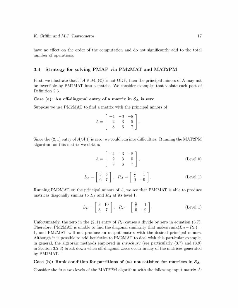
3.4 Strategy for solving PMAP via PM2MAT and MAT2PM

First, we illustrate that if A ∈ Mn(C) is not ODF, then the principal minors of A may notbe invertible by PM2MAT into a matrix. We consider examples that violate each part ofDefinition 2.3.

Case (a): An off-diagonal entry of a matrix in SA is zero

Suppose we use PM2MAT to find a matrix with the principal minors of

A =

−4 −3 −8

2 3 58 6 7

.

Since the (2, 1) entry of A/A[1] is zero, we could run into difficulties. Running the MAT2PMalgorithm on this matrix we obtain:

A =

−4 −3 −8

2 3 58 6 7

, (Level 0)

LA =

[3 56 7

], RA =

[32 10 −9

], (Level 1)

Running PM2MAT on the principal minors of A, we see that PM2MAT is able to producematrices diagonally similar to LA and RA at its level 1.

LB =

[3 103 7

], RB =

[32 10 −9

], (Level 1)

Unfortunately, the zero in the (2, 1) entry of RB causes a divide by zero in equation (3.7).Therefore, PM2MAT is unable to find the diagonal similarity that makes rank(LB −RB) =1, and PM2MAT will not produce an output matrix with the desired principal minors.Although it is possible to add heuristics to PM2MAT to deal with this particular example,in general, the algebraic methods employed in invschurc (see particularly (3.7) and (3.9)in Section 3.2.3) break down when off-diagonal zeros occur in any of the matrices generatedby PM2MAT.

Case (b): Rank condition for partitions of 〈m〉 not satisfied for matrices in SA

Consider the first two levels of the MAT2PM algorithm with the following input matrix A:


A =

2 −3 7 1 14 5 −3 1 14 −4 13 1 11 1 1 8 21 1 1 7 5

, (Level 0)

LA =

5 −3 1 1−4 13 1 11 1 8 21 1 7 5

, RA =

11 −17 −1 −12 −1 −1 −152 −5

2152

32

52 −5

2132

92

. (Level 1)

Note that

rank(LA[{1, 2}, {3, 4}]) = rank(LA[{3, 4}, {1, 2}]) = 1rank(RA[{1, 2}, {3, 4}]) = rank(RA[{3, 4}, {1, 2}]) = 1

where α = {1, 2} and β = {3, 4} form a partition of 〈4〉.

When PM2MAT is run with the principal minors of A as input, we produce the followingmatrices for level 1:

LB =

5 125 − 4

65 − 165

5 13 113

152

−654 13 8 7

4−65 52 8 5

, RB =

11 −3411 − 5

11 −1333

11 −1 −52 −13

6112 −1 15

21310

16526 −15

13152

92

. (Level 1)

One may verify that LA and LB have the same principal minors. Likewise, RA and RB havethe same principal minors. However, since the conditions of Theorem 3.1 are not satisfiedfor LA, LB need not be diagonally similar with transpose to LA, and indeed this is the case.When solving the 3 sets of quadratics to make the lower right 3× 3 submatrix of LB −RB

rank 1, there are two combinations of solutions that both make rank(LB(1) − RB(1)) = 1.By chance, the wrong solution is chosen, so the computation fails for the matrices as awhole. Solving the quadratics of equation (3.7) for the rest of the entries of the matricesdoes not yield a combination of solutions that makes rank(LB − RB) = 1.

By coincidence, RA and RB are diagonally similar with transpose, but the L matrices notbeing diagonally similar with transpose is sufficient to cause the computations of invschurcto fail.

Although this example suggests that (c) may imply (b) under the condition of (a) of Defi-nition 2.3, the converse is certainly not true as the following example shows.

Case (c): There exist multiple solutions which make rank(L − R)= 1

Similar to the last case, the operation of MAT2PM on A ∈ M4(R) is summarized below


down to level 2.

A =

3 −6 −9 121 3 −7 −4

32 2 −1 −16

93 1 1 4

, (Level 0)

LA =

3 −7 −4

32 −1 −16

91 1 4

, RA =

5 −4 −16

36 5 −88

97 10 −8

, (Level 1)

[−1 −16

91 4

],

[5 −88

910 −8

],

[113 −8

9103

409

],

[495 −152

45785 − 8

15

]. (Level 2)

Running PM2MAT on the principal minors of A above yields:[−1 16

9−1 4

],

[5 −176

95 −8

],

[113 −80

99113

409

],

[495 −3952

735495 − 8

15

], (Level 2)

LB =

3 −14

389

3 −1 169

−32 −1 4

, RB =

5 −14

5 −11215

607 5 −176

95 5 −8

, (Level 1)

B =

3 92

92 12

−43 3 −14

389

−4 3 −1 169

3 −32 −1 4

. (Level 0)

Although LA is diagonally similar to LB and RA is diagonally similar to RB , there are twosolutions that make rank(LB − RB) = 1. Instead of choosing the dot similarity with RB

R1 =

5 −8

3329

9 5 889

−212 −10 −8

which has determinant 712/3 like RA and RB, the dot similarity

R2 =

5 −8

3569

9 5 1609

−6 −112 −8

with determinant 260 is chosen, which also satisfies rank(LB − R2) = 1. Therefore, theresulting B which is computed with R2 above is not diagonally similar to A. In fact, B isdiagonally similar to

C =

3 -3 -9/2 12

2 3 −7 −4/3

4 2 −1 −16/93 1 1 4


where only the boxed entries differ from A. The principal minors of C (and B) are the sameas the principal minors of A with the exception of the determinant. Note that the outputof PM2MAT in this example is dependent on small round-off errors which may vary fromplatform to platform.

Although it would be easy to add code to PM2MAT to resolve this ambiguity for the casethat L,R ∈ M3(C), in general, the method of invschurc which finds solutions for makingrank(L − R) = 1 by working from the trailing 3 × 3 submatrix of L and R and progressingtowards the upper right (see equation (3.10)) is not well suited to also preserving diagonalsimilarity with transpose in cases where (c) of Definition 2.3 is not satisfied.

If the input principal minors do come from a matrix which is ODF, then PM2MAT willsucceed in building a matrix that has them as principal minors up to numerical limitations.The following proposition states this formally:

Proposition 3.7 Let pm ∈ C2n−1, n ∈ N be given. Suppose A ∈ Mn(C) is ODF. If

MAT2PM(A) = pm and B =PM2MAT(pm), then MAT2PM(B) = pm.

Proof. Let C ∈ Mm(C),m ≥ 2 be any submatrix or Schur complement produced byrunning MAT2PM on A (C ∈ SA). Since A is ODF, C has no off-diagonal zero entries andthus

L − R = C(1) − C/C[1] = C(1, 1]C[1, 1)/C[1]

has no zero entries. Hence, rank(L − R) 6= 0 for all such C.

Level n− 1 can always be created which matches the output of level n− 1 of MAT2PM(A)exactly, since this level of 1×1 matrices just consists of ratios of principal minors, where zeroprincipal minors can be handled using the multilinearity of the determinant (see Section3.2.4).

For all the 2×2 matrices of level n−2, rank(L−R) 6= 0 for each matrix we produce, so we areable to compute matrices which have the same principal minors as each of the corresponding2 × 2 matrices of level n − 2 we get from running MAT2PM on A. By Corollary 3.3, thematrices produced by PM2MAT are diagonally similar with transpose to the ones producedby MAT2PM, so by solving equations of the form of (3.7) (which always have solutionssince if A is ODF, division by zero never occurs) we can modify R so rank(L − R) = 1 foreach matrix of this level.

For subsequent levels, conditions (a) and (b) of Definition 2.3 guarantee that a diagonalsimilarity with transpose for all the R matrices exists so that rank(L−R) = 1 for each L,Rpair. Furthermore, condition (c) of the same definition guarantees that the dot similarityfound by invschurc is sufficient to find this (unique, if L is regarded as fixed) similarity.

Proceeding inductively we see that the final matrix B output by PM2MAT has the sameprincipal minors as A, since B has the same (1, 1) entry as A, L = B(1) is diagonally similar


with transpose to A(1) and R = B/B[1] is diagonally similar with transpose to A/A[1]. TheMAT2PM algorithm can then be used to verify that B and A have identical correspondingprincipal minors. �

Note that identical reasoning extends the result above to effectively ODF matrices.

If the input principal minors do not come from an effectively ODF matrix, PM2MAT mayfail to produce a matrix with the desired principal minors. If the input principal minors areinconsistent, that is, a matrix which has them as principal minors does not exist, PM2MATwill always fail to produce a matrix with the input principal minors.

When PM2MAT fails due to either inconsistent principal minors or due to principal minorsfrom an non-ODF matrix, it produces a matrix which does not have all the desired principalminors; no warning that this has occurred is guaranteed, since the warnings in PM2MATdepend upon numerical thresholds.

This suggests the following strategy for attempting to solve PMAP with principal minorsfrom an unknown source with PM2MAT.

1. PM2MAT is run on the input principal minors and an output matrix A is produced.

2. Then, MAT2PM is run on the matrix A, producing a second set of principal minors.

3. These principal minors are compared to the original input principal minors. If they agreeto an acceptable tolerance, PM2MAT succeeded. Otherwise, the principal minors are eitherinconsistent or they are not realizable by a matrix which is effectively ODF.

A sample implementation of this strategy is provided in PMFRONT in Appendix B.

4 Illustrative examples

Example 4.1 We obtain a moderately scaled set of integer principal minors that corre-spond to a real matrix. To do this, we use MAT2PM to find the principal minors of

A =

−6 3 −9 4−6 −5 3 6

3 −3 6 −71 1 −1 −3

,

yielding

pm =

1 2 3 4 5 6 7

[1] [2] [1, 2] [3] [1, 3] [2, 3] [1, 2, 3]−6 −5 48 6 −9 −21 −36

8 9 10 11 12 13 14 15[4] [1, 4] [2, 4] [1, 2, 4] [3, 4] [1, 3, 4] [2, 3, 4] [1, 2, 3, 4]−3 14 9 −94 −25 96 59 6

.


For ease of reference, the first row of the above displayed pm contains the index of a givenprincipal minor, the second row is the index set used to obtain the submatrix correspondingto that minor, while the third row contains the value of the principal minor itself. Forconvenience, the utility PMSHOW in Appendix G has been included, which produces outputsimilar to this for any input set of principal minors. To actually call PM2MAT, pm is justthe vector of values in the third row. Thus we can easily see that pm13 = det(A[1, 3, 4]) = 96,for example.

Since there are 24 − 1 entries in pm, we desire to find a matrix B ∈ M4(R) which hasthe values in pm as its principal minors. We begin with level = 3 and produce matricesequivalent in all principal minors at each level to the ones that would have been producedby running MAT2PM on A.

Level 3

At level 3 we desire to find eight 1 × 1 matrices whose entries are just the pivots in binaryorder. Since the principal minors are stored in binary order (see Definition 3.4 and [2,Proposition 4.6]) we compute the following quotients of consecutive principal minors:

pm8 = det(A[4]) = −3,pm9

pm1=

det(A[1, 4])

det(A[1])= −7

3, . . . ,

pm15

pm7=

det(A[1, 2, 3, 4])

det(A[1, 2, 3])= −1

6.

Therefore, the desired level 3 matrices are

[−3], [−73 ], [−9

5 ], [−4724 ], [−25

6 ], [−323 ], [−59

21 ], [−16 ].

Level 2

Analogously to the previous level, we can now compute the four pivots of the four 2 × 2matrices from the eight matrices of the previous level:

pm4 = 6,pm5

pm1=

3

2,

pm6

pm2=

21

5,

pm7

pm3= −3

4.

Since the first four 1× 1 matrices of the previous level are submatrices of the four matriceswe desire to compute, we know that these matrices have the form

B =

[6 ∗∗ −3

],

[32 ∗∗ −7

3

],

[215 ∗∗ −9

5

],

[−3

4 ∗∗ −47

24

],

where the ∗’s indicate entries not yet known. Consider producing the first of these matrices,labeled B and partitioned as follows:

B =

[B[1] B[1, 1)

B(1, 1] B(1)

].

From level 3 we know L = B[1] = −3 and R = B/B[1] = −25/6. Following equation (3.2),

L − R = −3 + 25/6 = 7/6 = B(1, 1]B[1, 1)/B[1].


Taking B[1, 1) = 7/6, we satisfy the equation above with B(1, 1] = B[1]. Thus we havecomputed

B =

[6 7

66 −3

].

Repeating this procedure for the other three matrices we finish level 2 with the followingfour matrices:

[6 7

66 −3

],

[32

253

32 −7

3

],

[215

106105

215 −9

5

],

[−3

4 −4324

−34 −47

24

].

Level 1

Computing the two pivots for the matrices of this level, we get pm2 = −5 and pm3/pm1 =48/ − 6 = −8. Thus, we seek to complete the matrices

C =

−5 ∗ ∗∗ 6 7

6∗ 6 −3

,

−8 ∗ ∗∗ 3

2253

∗ 32 −7

3

.

We label the first of these two matrices C, and we call invschurc with

L = C(1) =

[6 7

66 −3

], R = C/C[1] =

[215

106105

215 −9

5

]

from the previous level. Since

L − R ≈[

1.8 .15711.8 −1.2

]

is not rank one, we seek a t ∈ R such that equation (3.6) is satisfied. Solving equation (3.7),we find solutions t1 = 4/7, t2 = 106/49. Using t1,

L − R =

[6 7

66 −3

]−

[215

5330

125 −9

5

]=

[95 −3

5185 −6

5

].

Letting C[1, 1) = (L − R)[{1}, {1, 2}] = [−9/5,−3/5], we solve equation (3.2) to find

C(1, 1] =

[−5−10

],

so

C =

−5 9

5 −35

−5 6 76

−10 6 −3

.


Performing similar operations for the second matrix of level 1, we leave level 1 with the two3 × 3 matrices

−5 9

5 −35

−5 6 76

−10 6 −3

,

−8 9

4 −58

−8 32

253

−245

32 −7

3

.

Level 0

Given pivot = B[1] = pm1 = −6 and

L = B(1) =

−5 9

5 −35

−5 6 76

−10 6 −3

, R = B/B[1] =

−8 9

4 −58

−8 32

253

−245

32 −7

3

,

we desire to find the 4 matrix B of the form

B =

−6 ∗ ∗ ∗∗ −5 9

5 −35

∗ −5 6 76

∗ −10 6 −3

.

As in the previous level, rank(L − R) 6= 1, so we find r, s, t, such that equation (3.8) issatisfied. Solving equation (3.7) for each 2×2 submatrix of L−R, we obtain two quadraticsolutions for r, s and t:

r1 = 20/7, r2 = 10, s1 = 5/2, s2 = 5/16, t1 = 25/36, t2 = 25/8.

Then, comparing equation (3.9) for each of the 8 possible combinations, we find that onlyr = r2, s = s2, t = t2 makes rank(L − R) = 1. Applying this r, s, and t to R we obtain aR which is dot similar to R:

R =

−8 9

4s− 5

8t

−8s 32

253r

−24t5

3r2 −7

3

=

−8 36

5 −15

−52

32

56

−15 15 −73

.

In this case, R = D R D−1 with

D =

1 0 00 5

16 00 0 25

8

,

and no transpose is necessary.

Now,

L − R =

−5 9

5 −35

−5 6 76

−10 6 −3

−

−8 36

5 −15

−52

32

56

−15 15 −73

=

3 −27

5 −25

−52

92

13

5 −9 −23

.


Since 9/2 of row 2 is the maximum absolute diagonal entry of L − R, we let B[1, 1) =(L − R)[2, {1, 2, 3}] = [−5/2, 9/2, 1/3] and by equation (3.2) we find

B(1, 1] =

365−612

,

so

B =

−6 −52

92

13

365 −5 9

5 −35

−6 −5 6 76

12 −10 6 −3

.

Of course B is not equal to the original matrix A, but A = DBD−1 where

D =

1 0 0 00 −5

6 0 00 0 −1

2 00 0 0 1

12

.

For simplicity of illustration, the deskewing of Section 3.2.5 has not been applied to theoutput matrix B.

Example 4.2 To show how zero principal minors are handled as discussed in Section 3.2.4,we consider running PM2MAT on the principal minors of the effectively ODF matrix

A =

2 2 52 2 −37 3 −1

.

Using the convention of Example 4.1, A has principal minors:

pm =

1 2 3 4 5 6 7

[1] [2] [1, 2] [3] [1, 3] [2, 3] [1, 2, 3]2 2 0 −1 −37 7 −64

.

The 1 × 1 matrices of level 2 consist of the ratios

[pm4], [pm5/pm1], [pm6/pm2], [pm7/pm3]. (Level 2)

Since pm3 = 0, building these matrices would fail if the zero principal minor code were notinvoked.

The goal of zero principal minor loop at the beginning of PM2MAT is to create a consistent(taking into account the modified pivot entries) set of principal minors where the initial


2n−1 − 1 principal minors are nonzero. It does this by making all the pivot or (1, 1) entriesof the matrices that correspond to zero principal minors have pivots equal to ppivot insteadof zero.

In the example at hand, we will take ppivot = 1 for simplicity. Since pm3 is computedby knowing that the pivot entry of the right matrix of level 1 is pm3/pm1, we assignpm3 = ppivot · pm1 = 1 · 2 = 2. Of course, in general, changing a single principal minordoes not even result in a set of principal minors that are consistent, so the next part of thezero principal minor loop is devoted to computing the sums of principal minors that followfrom applying the multilinearity of the determinant (also see the discussion of zero pivotsin [2]) to the change just made. Since pm3 is found from the (1, 1) entry of A/A[1], onlyprincipal minors from descendants (in the top to bottom sense of the tree of Figure 1) of theSchur complement of A/A[1] need to change. The only principal minor that satisfies thiscondition is pm7. Thus, the remaining required change to the vector of principal minors isto let pm7 = pm7 + ppivot · pm5 = −64 + (−37) = −101. The final set of principal minorsthat we enter the main loop of PM2MAT is then

nzpm =

1 2 3 4 5 6 7

[1] [2] [1, 2] [3] [1, 3] [2, 3] [1, 2, 3]2 2 2 −1 −37 7 −101

,

where nzpm signifies “nonzero principal minors”. The first two levels of PM2MAT thenyield

[−1], [−37/2], [7/2], [−101/2], (Level 2)

L =

[2 −9

22 −1

], nzR =

[ppivot = 1 32

1 −372

]. (Level 1)

At this point we recall that nzpm was designed to create ppivot = 1 in the (1, 1) entry ofthe matrix nzR, but the original principal minors corresponded to the (1, 1) entry of nzRbeing zero. Subtracting ppivot = 1 from nzR[1] and continuing we obtain:

L =

[2 −9

22 −1

], R =

[0 321 −37

2

], (Level 1)

B =

2 −10

3352

−65 2 −9

22 2 −1

. (Level 0)

Note that B is diagonally similar to A with transpose, and thus has the principal minorspm. If we had continued to run PM2MAT with the level 1 matrix nzR, we would haveobtained a matrix that had the principal minors nzpm instead.


Example 4.3 To show that PM2MAT may succeed in producing an output matrix whichis not diagonally similar with transpose to another matrix having the same principal minors,consider running PM2MAT on the principal minors of

A =

2 4 1 13 5 1 11 1 7 131 1 6 −3

which are

pm = [2, 5,−2, 7, 13, 34,−14,−3,−7,−16, 6,−99,−183,−480, 198].

This matrix is not ODF by (c) of Definition 2.3, but it is structured so that regardless ofwhich dot similarity is chosen to make the final 3×3 difference of L and R rank 1, a matrixwith the same principal minors results. By chance, PM2MAT returns the matrix

B =

2 6 25

1235

2 5 15

635

52 5 7 78

73512

356 7 −3

(before deskewing) which is not diagonally similar with transpose to A. Note that in thisexample, the output of PM2MAT is dependent on small round-off errors which may varyfrom platform to platform, although the principal minors of the output matrix will bevirtually the same regardless.

5 A polynomial time algorithm

As the size n of the matrix A ∈ Mn(C) increases, A has many more principal minors thanentries. We thus know that these principal minors are dependent on each other. To studysome of these dependencies, we prove the following preliminary result.

Lemma 5.1 Let A ∈ Mn(C), n ≥ 4, have 2n−1 principal minors {pm1, pm2, . . . , pm2n−1}.If A is ODF, then pm2n−1 is determined by {pm1, pm2, . . . , pm2n−2}.

Proof. Let {pm1, pm2, . . . , pm2n−2, pm2n−1} be passed to PM2MAT where pm2n−1 6=pm2n−1 and for convenience pm2n−1 6= 0. The proof proceeds by showing that the 4 × 4matrices of level n − 4 using this set of principal minors with the last principal minormodified will be identical to those 4 × 4 matrices of level n − 4 we would have obtainedusing the original principal minors {pm1, pm2, . . . , pm2n−2, pm2n−1}.


The queue of 1 × 1 matrices of level n − 1 will be identical to the queue of 1 × 1 matricesof level n − 1 using the original principal minors {pm1, pm2, . . . , pm2n−2, pm2n−1} exceptfor the last value. Therefore, the queue of 2 × 2 matrices of level n − 2 will be identical tothe same queue using the original principal minors except for the final matrix, whose (1, 2)entry will be different. Let

R =

[r11 r12

r21 r22

]

be the last matrix of level n−2. Let B be the last matrix of level n−3 we desire to producefrom level n − 2 and as usual we have R = B/B[1] and L = B(1). When we solve thequadratic equation (3.7) and modify R so that rank(L − R) = 1, we have

C = L − R =

[c11 c12

c21 c22

],

where only c12 and c21 are different from entries we would have obtained using the originalprincipal minors. Note, however, that rank(L−R) = rank(C) = 1 implies that det(C) = 0,so in fact c12 c21 = c12 c21. Hence, C is diagonally similar to the matrix we would haveobtained using the original principal minors. Although B will be different from the B wewould have obtained with the original principal minors, it will only be different in its (1, 3)and (3, 1) entries (or (1, 2) and (2, 1) entries, depending on the relative magnitudes of c11

and c22 by Equations (3.3), (3.4) and (3.5)), while the product of these entries will be thesame. Since A is ODF and B is dot similar to the corresponding Schur complement of A,there will only be one dot similarity with B that will make the difference of B with itscorresponding left matrix rank 1 (see (c) of Definition 2.3). Therefore, all the 4×4 matricesof level n−4 will be identical to those that were obtained using the original principal minors.�

Example 5.2 To illustrate the above lemma, let us revisit Example 4.1 from Section 4.The operation of PM2MAT is summarized as follows:

pm = [−6,−5, 48, 6,−9,−21,−36,−3, 14, 9,−94,−25, 96, 59, 6]

[−3], [−73 ], [−9

5 ], [−4724 ], [−25

6 ], [−323 ], [−59

21 ], [−16 ] (Level 3)

[6 7

66 −3

],

[32

253

32 −7

3

],

[215

106105

215 −9

5

],

[−3

4 −4324

−34 −47

24

](Level 2)

−5 9

5 −35

−5 6 76

−10 6 −3

,

−8 9

4152

−8 32

253

25

32 −7

3

(Level 1)

−6 −52

92

13

365 −5 9

5 −35

−6 −5 6 76

12 −10 6 −3

(Level 0)


If instead we use the input (entries that are different are in bold)

pm = [−6,−5, 48, 6,−9,−21,−36,−3, 14, 9,−94,−25, 96, 59,1]

we obtain

[−3], [−73 ], [−9

5 ], [−4724 ], [−25

6 ], [−323 ], [−59

21 ], [− 1

36] (Level 3)

[6 7

66 −3

],

[32

253

32 −7

3

],

[215

106105

215 −9

5

],

[−3

4 −139

72

−34 −47

24

](Level 2)

−5 9

5 −35

−5 6 76

−10 6 −3

,

−8 9

4 −0.6304 . . .−8 3

2253

−4.7590 . . . 32 −7

3

(Level 1)

−6 −52

92

13

365 −5 9

5 −35

−6 −5 6 76

12 −10 6 −3

(Level 0)

Rational expressions for the (1, 3) and (3, 1) entries of the last matrix of level 1 do not exist,but note that (15/2) · (2/5) = 3 ≈ (−0.6304) · (−4.7590).

As a consequence to Lemma 5.1 we observe that generically all the “large” principal minorsof a matrix can be expressed in terms of the “small” principal minors.

Theorem 5.3 Let A ∈ Mn(C), n ≥ 4. If A is ODF, each principal minor which is indexed

by a set with 4 or more elements can be expressed in terms of the principal minors which

are indexed by 3 or fewer elements.

Proof. Consider all the submatrices of A indexed by exactly 4 elements. Applying Lemma5.1 to each of them, we see that all of the principal minors indexed by exactly 4 elementsare functions of all the smaller principal minors (the determinants of all 1×1, 2×2 and 3×3principal submatrices of A). Applying Lemma 5.1 to each principal minor of A indexed byexactly 5 elements, these are functions of all of the principal minors indexed by 4 or fewerelements. However, all the principal minors with exactly 4 elements are functions of theprincipal minors indexed by 3 or fewer elements, so all the principal minors indexed by 5elements are functions of the principal minors indexed by 3 or fewer elements. The resultfollows by induction. �

As a result of Theorem 5.3 we see that if A ∈ Mn(C) is ODF, then there does not exist aB ∈ Mn(C) not diagonally similar with transpose to A such that A and B have the same1 × 1, 2 × 2 and 3 × 3 principal minors.


Theorem 5.3 motivates a “fast” version of PM2MAT that only takes as inputs the 1 × 1,2 × 2 and 3 × 3 principal minors but produces the same output matrix as PM2MAT if theinput principal minors come from a ODF matrix. To this end, a matching, fast (polynomialtime) version of MAT2PM was written to produce only these small principal minors and isdescribed first.

FMAT2PM

For a ODF matrix of size n, there are only

(n1

)+

(n2

)+

(n3

)= n +

n(n − 1)

2+

n(n − 1)(n − 2)

6=

n(n2 + 5)

6

principal minors with index sets of size ≤ 3 on which all the other principal minors depend.A fast and limited version of MAT2PM was implemented that produces only these principalminors in the function FMAT2PM in Appendix C. Instead of having 2k matrices at eachlevel which yield 2k principal minors at level = k, there are only

(k2

)+

(k1

)+

(k0

)=

k(k + 1)

2+ 1 (5.13)

matrices that need be computed resulting in the corresponding number of principal minorsbeing produced. This is because at level = k we only need to compute those principalminors involving the index k + 1 and 2 smaller indices to produce the principal minorswhich come from 3 × 3 submatrices. The other two terms of (5.13) are similarly derived:the k + 1 index and 1 smaller index is used to compute the principal minors which comefrom 2 × 2 submatrices, and each level has one new minor from the 1 × 1 submatrix whichis referenced by the index k + 1.

From (5.13), it is easily verified that at each level = k, precisely k more matrices areproduced than were computed at level = k − 1.

Simple logic can be used to determine which matrices in the input queue need to be processedto produce matrices in the output queue. If the (1, 1) entry of a matrix corresponds to aprincipal minor with an index set of 2 or less (a 2×2 or 1×1 principal minor) then we takethe submatrix and Schur complement of the matrix, just as we do in MAT2PM since thismatrix will have descendants which correspond to principal minors from 3× 3 submatrices.However, if the (1, 1) entry of a matrix corresponds to a principal minor with an index setof 3, then we only take the submatrix of this matrix; no Schur complement is computedor stored. This scheme prevents matrices that would be used to find principal minors withan index set of 4 or more from ever being computed. To keep track the index sets ofthe principal minors, the index of the principal minor as it would have been computed inMAT2PM is stored in the vector of indices pmidx. In the code, the MAT2PM indices inpmidx are referred to as the long indices of a principal minor, while the indices in the pmvector produced by FMAT2PM are called the short indices of a given principal minor. The


vector of long indices pmidx is output along with the vector of principal minors in pm byFMAT2PM.

At each level, the indices pertaining to the principal minors which are computed at thatlevel are put in pmidx. The following table shows how pmidx is incrementally computedat each level:

level pmidx

0 [1, 0, 0, . . . , 0]

1 [1, 2, 3, 0, 0, . . . , 0]

2 [1, 2, 3, 4, 5, 6, 7, 0, . . . , 0]

3 [1, 2, 3, 4, 5, 6, 7, 8, 9, 10, 11, 12, 13, 14, 0, . . . , 0]

4 [1, 2, 3, 4, 5, 6, 7, 8, 9, 10, 11, 12, 13, 14, 16, 17,18, 19, 20, 21, 22, 24, 25, 26, 28, 0, . . . , 0]

......

As an aid to interpreting the values in pmidx, the utilities IDX2V and V2IDX in AppendixF and Appendix E respectively have been included. IDX2V takes a long index in pmidxand produces the index set of the submatrix that corresponds to it and returns this as avector. V2IDX is the inverse of this operation.

We note that FMAT2PM could be adapted analogously to compute all principal minors upto any fixed size of index set.

FPM2MAT

Given pm and pmidx in the format produced by FMAT2PM, FPM2MAT can invert onlythese 1 × 1, 2 × 2 and 3 × 3 principal minors into a matrix that is unique up to diagonalsimilarity with transpose if the principal minors come from a matrix which is ODF as aconsequence of Theorem 5.3.

It is not strictly necessary that pmidx be an input to FPM2MAT since it is fixed for anygiven matrix size n, but since pmidx is produced naturally by FMAT2PM and since pmidxcan be thought of with pm as implementing a very sparse vector format, pm and pmidx areinput together to FPM2MAT.

Since FPM2MAT processes levels from the largest (bottom) to smallest (top), it was usefulto make the vector ipmlevels at the beginning of FPM2MAT which contains the short indexof the beginning of each level. Then, at each level, FPM2MAT computes those matriceswhich have a submatrix (or left matrix L). If a Schur complement (an R matrix) existsfor the matrix to be produced, this is input to invschurc just as in PM2MAT. Otherwise,a matrix of ones is passed in for the Schur complement to invschurc, since the particularvalues will prove to be of no consequence (see Example 5.2). Although this is slightly slowerthan just embedding L in a larger matrix, it has been found to produce more accurate results


for large n.

The bulk of the operations of FPM2MAT including the subroutines invschurc, solverightand deskew are unchanged from PM2MAT.

5.1 Notes on the operation of the fast versions

• FMAT2PM processes a 53 × 53 matrix in about the same time that MAT2PM canprocess a 20 × 20 matrix.

• FPM2MAT can invert the 24857 “small” principal minors of a 53×53 real or complexmatrix into a matrix in M53 in a few minutes.

• Zero principal minors are not presently handled by either FMAT2PM or FPM2MATfor clarity of presentation, but the multilinearity of the determinant could be exploitedin these programs to handle zero principal minors as is implemented in MAT2PM andPM2MAT.

• For FMAT2PM, only k + 1 matrices need to have Schur complements taken at eachlevel = k. Thus, FMAT2PM is of order O(n4 ) since

n−2∑

k=0

(k + 1)2(n − (k + 1))2 =1

6(n4 − n2),

where there are generally 2 operations for each element of the Schur complement. Thescaling of the outer product by the inverse of the appropriate principal minor onlyaffects (n − (k + 1)) elements at level k.

• It has been found that for numerical reasons it is desirable to call invschurc with adummy matrix of ones whenever the R Schur complement matrix is missing.

• To find the approximate operation count for FPM2MAT, we note that the quadratics(3.7) need to be solved for each upper triangular entry of each of the k(k + 1)/2 + 1matrices (see (5.13)) at each level = k. As in (3.11) we let q be the number ofoperations to solve the quadratic equation to find

n−2∑

k=0

(k(k +1)/2+1)(n− (k +1))(n− (k +2))q/2 =q

120(n5 −5n4 +25n3 −55n2 +34n).

Similarly, letting p be the number of operations to evaluate equations of the form(3.9),

pn−3∑

k=0

(k(k + 1)/2 + 1)(8 + 4(n − (k + 3)) + (n − (k + 2))(n − (k + 3))) =

p

60(n5 + 35n3 − 180n2 + 504n − 600),


as in the sum of (3.12). Thus, FPM2MAT is O(n5 ).

6 Some consequences and remarks

In this section we will touch upon some subjects and problems related to PMAP andPM2MAT in the form of remarks.

Remark 6.1 With PM2MAT we can at least partially answer a question posed by Holtzand Schneider in [3, problem (4) p. 265-266]. The authors pose PMAP as one step towardthe inverse problem of finding a GKK matrix with prescribed principal minors.

Given a set of principal minors, we can indeed determine via PM2MAT whether or not thereis an effectively ODF matrix A that has them as its principal minors. To accomplish this,we simply run PM2MAT on the given set of principal minors, producing a matrix A. Then,we run MAT2PM on this matrix to see if the matrix A has the desired principal minors. Ifthe principal minors are consistent and belong to an effectively ODF matrix, the principalminors will match, up to numerical limitations. If the principal minors cannot be realizedby a matrix or if the principal minors do not belong to an effectively ODF matrix, thenthe principal minors of A will not match the input principal minors. In the former case,the generalized Hadamard-Fischer inequalities and the Gantmacher-Krein-Carlson theorem(see [3]) can be used to decide whether there is a GKK and effectively ODF matrix withthe given principal minors.

Remark 6.2 In Stouffer [6], it is claimed that for A ∈ Mn(C) there are only n2 − n + 1“independent” principal minors that all the other principal minors depend on, and as thefirst example of such a “complete” set the following set is offered:

S = {A[i] : i ∈ 〈n〉} ∪ {A[i, j] : i < j; i, j ∈ 〈n〉} ∪ {A[1, i, j] : i < j; i, j ∈ {2, 3, . . . , n}}.

Indeed, S contains (n1

)+

(n2

)+

(n − 1

2

)= n2 − n + 1

principal minors. However, these principal minors are not independent since equations [6,(5) and (6), p. 358] may not even have solutions if the principal minors are not consistent orcome from a matrix which is not ODF. Moreover, even generically, S does not determine Aup to diagonal similarity with transpose for n ≥ 4 since, in general, the last two equationsof [6, (6), p. 358] have two solutions for each aij , aji pair. The set S in [6], however, doesgenerically determine the other principal minors of A up to a finite set of possibilities.

Remark 6.3 The conditions of Definition 2.3 are difficult to verify from an input set ofprincipal minors from an unknown source without actually running the PM2MAT algorithm


on them. In particular, part (c) is difficult to verify even if a matrix that has the sameprincipal minors as the input principal minors happens to be known. However, usuallyPM2MAT will print a warning if the conditions of the definition are not satisfied, and thestrategy of Section 3.4 can be employed to quickly verify if PM2MAT has performed thedesired task.

Remark 6.4 Note that Theorem 5.3 does not imply that the principal minors indexed by3 or fewer elements are completely free. There are additional constraints among the smallerprincipal minors. If one chooses a set of principal minors indexed by 3 or fewer elementsat random and uses FPM2MAT to invert these into a matrix A, the matrix A will not ingeneral have the same principal minors indexed by 3 or fewer elements as the input principalminors.

Remark 6.5 If a random vector of principal minors is passed to PM2MAT, the resultingmatrix will have all the desired 1 × 1 and 2 × 2 principal minors, and some of the 3 × 3principal minors will be realized as well. However, none of the larger principal minors willbe the same as those that were in the input random vector of principal minors.

7 Future work

Here we summarize some of our main goals for the future regarding PMAP and PM2MAT.

• Incorporate into PMAP and its solution algorithm structural and qualitative require-ments of the matrix solutions. For example, we may want to seek solutions of specialstructure (e.g., positive definite, Hessenberg, Toeplitz) or having other special at-tributes (e.g., specified directed graph, entrywise nonnegativity).

• Expand the functionality of PM2MAT from effectively ODF matrices to a broaderclass of matrices.

• Identify applications of PMAP in theoretical and applied mathematics, and contributeto the solution of relevant problems.

• Examine the potential consequences and usage of our algorithmic approach to theP-problem. This the problem of checking whether a given matrix is a P-matrix ornot. Recall that a P-matrix is one all of whose principal minors are positive. TheP-problem is known to be an NP-hard problem [1].

To be more specific, note all the principal minors that FMAT2PM computes beingpositive provides a polynomial time necessary condition for a matrix to be a P-matrix.If the positivity of the larger minors could be predicted from these 1×1, 2×2 and 3×3principle minors for ODF matrices, then it would be possible to realize a polynomialtime algorithm for the P-problem applied to this class of matrices.


Acknowledgment

The authors are grateful to an anonymous referee for a careful examination of the first draftof this paper leading to the introduction of condition (c) of Definition 2.3 and for severalother improvements to the manuscript.

References

[1] G. E. Coxson, The P-matrix problem is co-NP-complete, Mathematical Programming,64 : 173–178, 1994.

[2] K. Griffin and M.J. Tsatsomeros. Principal Minors, Part I: A method for computingall the principal minors of a matrix. Submitted to Linear Algebra and Its Applications.

[3] O. Holtz and H. Schneider. Open problems on GKK τ -matrices. Linear Algebra and

its Applications, 345:263-267, 2002.

[4] R. Loewy. Principal Minors and Diagonal Similarity of Matrices. Linear Algebra and

Its Applications, 78:23–64, 1986.

[5] D. V. Ouellette. Schur Complements and Statistics. Linear Algebra and Its Applica-

tions. 36:187–295, 1981.

[6] E. B. Stouffer, On the Independence of Principal Minors of Determinants, Transactions

of the American Mathematical Society. Vol. 26 No. 3 356–368, (July 1924).


A PM2MAT

% PM2MAT Finds a real or complex matrix that has PM as its principal

% minors.

%

% PM2MAT produces a matrix with some, but perhaps not all, of its

% principal minors in common with PM. If the principal minors are

% not consistent or the matrix that has them is not ODF, PM2MAT will

% produce a matrix with different principal minors without warning.

% Run MAT2PM on the output matrix A as needed.

%

% A = PM2MAT(PM)

% where PM is a 2^n - 1 vector of principal minors and A will be an n x n

% matrix.

%

% The structure of PM, where |A[v]| is the principal minor of "A" indexed

% by the vector v:

% PM: |A[1]| |A[2]| |A[1 2]| |A[3]| |A[1 3]| |A[2 3]| |A[1 2 3]| ...

function A = pm2mat(pm)

myeps = 1e-10;

n = log2(length(pm)+1);

% Make first (smallest) entry of zeropivs an impossible index

zeropivs = 0;

% Pick a random pseudo-pivot value that minimizes the chances that

% pseudo-pivoting will create a non-ODF matrix.

ppivot = 1.9501292851471754e+000;

% initialize globals to allow warnings to be printed only once

global WARN_A WARN_C WARN_I

WARN_A = false; WARN_C = false; WARN_I = false;

% To avoid division by zero, do an operation analogous to the zeropivot

% loop in mat2pm.

for i = 1:((length(pm)+1)/2 - 1)

if (abs(pm(i)) < myeps)

mask = i;

zeropivs = union(zeropivs, i);

ipm1 = bitand(mask, bitcmp(msb(mask),48));

if ipm1 == 0

pm(mask) = pm(mask) + ppivot;

else

pm(mask) = (pm(mask)/pm(ipm1) + ppivot)*pm(ipm1);

end

delta = msb(mask);

delta2 = 2*delta;

for j = mask+delta2:delta2:2^n - 1


pm(j) = pm(j) + ppivot*pm(j - delta);

end

end

end

zeropivsidx = length(zeropivs) - 1;

zeropivsmax = zeropivs(zeropivsidx+1);

% initial processing is special, no call to invschurc is necessary

nq = 2^(n-1);

q = zeros(1,1,nq);

ipm1 = nq;

ipm2 = 1;

for i = 1:nq

if i == 1

q(1,1,i) = pm(ipm1);

else

q(1,1,i) = pm(ipm1)/pm(ipm2);

ipm2 = ipm2+1;

end

ipm1 = ipm1+1;

end

%

% Main ’level’ loop

%

for level = n-2:-1:0 % for consistency with mat2pm levels

[n1, n1, nq] = size(q);

nq = nq/2;

n1 = n1+1;

% The output queue has half the number of matrices, each one larger in

% row and col dimension

qq = zeros(n1, n1, nq);

ipm1 = 2*nq-1;

ipm2 = nq-1;

for i = nq:-1:1 % process matrices in reverse order for zeropivs

if (i == 1)

pivot = pm(ipm1);

else

pivot = pm(ipm1)/pm(ipm2);

ipm2 = ipm2-1;

end

qq(:,:,i) = invschurc(pivot, q(:,:,i), q(:,:,i+nq));

if zeropivsmax == ipm1

qq(1,1,i) = qq(1,1,i) - ppivot;

zeropivsmax = zeropivs(zeropivsidx);

zeropivsidx = zeropivsidx - 1;

end


ipm1 = ipm1-1;

end

q = qq;

end

A = q(:,:,1);

A = deskew(A);

if WARN_A

% ODF (a) not satisfied

fprintf(2,...

’PM2MAT: off diagonal zeros found, solution suspect.\n’);

end

if WARN_C

fprintf(2,...

’PM2MAT: multiple solutions to make rank(L-R)=1, solution suspect.\n’);

end

if WARN_I

fprintf(2, ...

’PM2MAT: input principal minors may be inconsistent, solution suspect.\n’);

end

%

% Suppose A is an (m+1) x (m+1) matrix such that

%

% pivot = A(1,1)

% L = A(2:m+1, 2:m+1)

% R = L - A(2:m+1,1)*A(1,2:m+1)/pivot = (the Schur’s complement with

% respect to the pivot or A/A[1]).

%

% Then invschurc finds such an (m+1) x (m+1) matrix A (not necessarily

% unique) given the pivot (a scalar), and the m x m matrices L and R.

%

% If rank(L-R) is not 1, modifies R so that L-R is rank 1.

%

function A = invschurc(pivot, L, R)

global WARN_C WARN_I

myeps_i = 1e-3*norm(R,inf); % make these relative to magnitude of R

myeps_c = 1e-9*norm(R,inf);

m = length(R);

% Try to make (L-R) rank 1

if m == 2

[t1,t2] = solveright(L(1,1), L(1,2), L(2,1), L(2,2),...

R(1,1), R(1,2), R(2,1), R(2,2));

% This is arbitrary, take the first.

t = t1;


R(2,1) = R(2,1)*t;

R(1,2) = R(1,2)/t;

elseif m >= 3

% We start with the lower right hand 3x3 submatrix. We have 3

% parameters, each with two possible solutions. Only 1 of the 8

% possible solutions need give us a L-R which is rank 1. We find the

% right solution by brute force.

i1 = m-2;

i2 = m-1;

i3 = m;

[r1,r2] = solveright(L(i2,i2), L(i2,i3), L(i3,i2), L(i3,i3),...

R(i2,i2), R(i2,i3), R(i3,i2), R(i3,i3));

[s1,s2] = solveright(L(i1,i1), L(i1,i2), L(i2,i1), L(i2,i2),...

R(i1,i1), R(i1,i2), R(i2,i1), R(i2,i2));

[t1,t2] = solveright(L(i1,i1), L(i1,i3), L(i3,i1), L(i3,i3),...

R(i1,i1), R(i1,i3), R(i3,i1), R(i3,i3));

% Perform a parameterized "row reduction" on the first two rows of this

% matrix and compute the absolute value of the (2,3) entry. One of

% them will be nearly zero.

r111 = abs((L(i2,i3) - R(i2,i3)/r1)*(L(i1,i1) - R(i1,i1)) - ...

(L(i2,i1) - R(i2,i1)*s1)*(L(i1,i3) - R(i1,i3)/t1));


(L(i2,i1) - R(i2,i1)*s1)*(L(i1,i3) - R(i1,i3)/t2));


(L(i2,i1) - R(i2,i1)*s2)*(L(i1,i3) - R(i1,i3)/t1));


(L(i2,i1) - R(i2,i1)*s2)*(L(i1,i3) - R(i1,i3)/t2));


(L(i2,i1) - R(i2,i1)*s1)*(L(i1,i3) - R(i1,i3)/t1));


(L(i2,i1) - R(i2,i1)*s1)*(L(i1,i3) - R(i1,i3)/t2));


(L(i2,i1) - R(i2,i1)*s2)*(L(i1,i3) - R(i1,i3)/t1));


(L(i2,i1) - R(i2,i1)*s2)*(L(i1,i3) - R(i1,i3)/t2));

rv = [r111, r112, r121, r122, r211, r212, r221, r222];

mn = min(rv);

if (r111 == mn)

r = r1; s = s1; t = t1;

elseif (r112 == mn)

r = r1; s = s1; t = t2;

elseif (r121 == mn)

r = r1; s = s2; t = t1;

elseif (r122 == mn)

r = r1; s = s2; t = t2;

elseif (r211 == mn)

r = r2; s = s1; t = t1;

elseif (r212 == mn)


r = r2; s = s1; t = t2;

elseif (r221 == mn)

r = r2; s = s2; t = t1;

else % (r222 == mn)

r = r2; s = s2; t = t2;

end

if mn > myeps_i

WARN_I = true;

end

if sum(rv < myeps_c) > 1

WARN_C = true;

end

R(i3,i2) = R(i3,i2)*r;

R(i2,i3) = R(i2,i3)/r;

R(i2,i1) = R(i2,i1)*s;

R(i1,i2) = R(i1,i2)/s;

R(i3,i1) = R(i3,i1)*t;

R(i1,i3) = R(i1,i3)/t;

% Now the lower right hand 3x3 submatrix of L-R has rank 1. Then we

% fix up the rest of L-R.

for i1 = m-3:-1:1

i2 = i1+1;

i3 = i1+2;

% Now the inside lower right submatrix is done, so we

% only have 2 free parameters and 4 combinations to examine.

[s1,s2] = solveright(L(i1,i1), L(i1,i2), L(i2,i1), L(i2,i2),...

R(i1,i1), R(i1,i2), R(i2,i1), R(i2,i2));

[t1,t2] = solveright(L(i1,i1), L(i1,i3), L(i3,i1), L(i3,i3),...

R(i1,i1), R(i1,i3), R(i3,i1), R(i3,i3));

r11 = abs((L(i2,i3) - R(i2,i3))*(L(i1,i1) - R(i1,i1)) - ...

(L(i2,i1) - R(i2,i1)*s1)*(L(i1,i3) - R(i1,i3)/t1));


(L(i2,i1) - R(i2,i1)*s1)*(L(i1,i3) - R(i1,i3)/t2));


(L(i2,i1) - R(i2,i1)*s2)*(L(i1,i3) - R(i1,i3)/t1));


(L(i2,i1) - R(i2,i1)*s2)*(L(i1,i3) - R(i1,i3)/t2));

rv = [r11, r12, r21, r22];

mn = min(rv);

if (r11 == mn)

s = s1; t = t1;

elseif (r12 == mn)

s = s1; t = t2;

elseif (r21 == mn)

s = s2; t = t1;


else % (r22 == mn)

s = s2; t = t2;

end

if mn > myeps_i

WARN_I = true;

end


WARN_C = true;

end

R(i2,i1) = R(i2,i1)*s;

R(i1,i2) = R(i1,i2)/s;

R(i3,i1) = R(i3,i1)*t;

R(i1,i3) = R(i1,i3)/t;

for j = i1+3:m

% Finally, once the second row of the submatrix we are working

% on is uniquely solved, we just pick the solution to the

% quadratic such that the the first row is a multiple of the

% second row. Note that one of r1, r2 will be almost zero.

% Solving the quadratics leads to much better performance

% numerically than just taking multiples of the second or

% any other row.

%

j1 = i1+1;

[t1,t2] = solveright(L(i1,i1), L(i1,j), L(j,i1), L(j,j),...

R(i1,i1), R(i1,j), R(j,i1), R(j,j));

r1 = abs((L(j1,j) - R(j1,j))*(L(i1,i1) - R(i1,i1)) - ...

(L(j1,i1) - R(j1,i1))*(L(i1,j) - R(i1,j)/t1));

r2 = abs((L(j1,j) - R(j1,j))*(L(i1,i1) - R(i1,i1)) - ...

(L(j1,i1) - R(j1,i1))*(L(i1,j) - R(i1,j)/t2));

if (r1 <= r2)

t = t1;

else

t = t2;

end

rv = [r1, r2];

if mn > myeps_i

WARN_I = true;

end


WARN_C = true;

end

R(j,i1) = R(j,i1)*t;

R(i1,j) = R(i1,j)/t;

end

end

end


B = (L-R); % a rank 1 matrix

[mn, idxmax] = max(abs(diag(B)));

% For numerical reasons use the largest diagonal element as a base to find

% the two vectors whose outer product is B*pivot

yT = B(idxmax,:);

if yT(idxmax) == 0

% This shouldn’t happen normally, but to prevent

% divide by zero when we set all "dependent" principal

% minors (with index sets greater than or equal to a constant)

% to the same value, let yT be something.

yT = ones(1,m);

end

x = B(:,idxmax)*pivot / yT(idxmax);

A = zeros(m+1);

A(1,1) = pivot;

A(1,2:m+1) = yT;

A(2:m+1,1) = x;

A(2:m+1,2:m+1) = L;

%

% Returns the two possible real solutions that will make L-R rank one if we

% let

% r21 = r21*t? (where ? = 1 or 2) and

% r12 = r12/t?

%

function [t1,t2] = solveright(l11,l12,l21,l22,r11,r12,r21,r22)

global WARN_A

x1 = l11-r11;

x2 = l22-r22;

d = sqrt(x1^2*x2^2 + l12^2*l21^2 + r12^2*r21^2 - 2*x1*x2*l12*l21 - ...

2*x1*x2*r12*r21-2*l12*l21*r21*r12);

if (l12 == 0)||(r21 == 0)

% This shouldn’t happen normally, but to prevent

% divide by zero when we set all "dependent" principal

% minors (with index sets greater than or equal to a constant)

% to the same value, let [t1,t2] be something.

t1 = 1;

t2 = 1;

WARN_A = true;

else

t1 = (-x1*x2 + l12*l21 + r12*r21 - d)/(2*l12*r21);

t2 = (-x1*x2 + l12*l21 + r12*r21 + d)/(2*l12*r21);

% This also shouldn’t happen. Comment above applies.

if (t1 == 0)||(t2 == 0)

WARN_A = true;

if (t1 == 0)&&(t2 == 0)


t1 = 1;

t2 = 1;

elseif (t1 == 0)

% return better solution in t1 for m=2 case in invschurc

t1 = t2;

t2 = 1;

else % (t2 == 0)

t2 = 1;

end

end

end

%

% Makes abs(A(1,i)) = abs(A(i,1)) through diagonal similarity for all i.

%

function A = deskew(A)

n = length(A);

d = ones(n,1);

for i = 2:n

if A(i,1) ~= 0 % don’t divide by 0

d(i) = sqrt(abs(A(1,i)/A(i,1)));

if (d(i) > 1e6)||(d(i) < 1e-6)

% something is likely wrong, use 1 instead

d(i) = 1;

end

end % else leave d(i) = 1

end

% If D = diag(d), this effectively computes A = D*A*inv(D)

for i = 2:n

A(i,:) = A(i,:)*d(i);

end

for i = 2:n

A(:,i) = A(:,i)/d(i);

end

% Returns the numerical value of the most significant bit of x.

% For example, msb(7) = 4, msb(6) = 4, msb(13) = 8.

function m = msb(x)

persistent MSBTABLE % MSBTABLE persists between calls to mat2pm

if isempty(MSBTABLE)

% If table is empty, initialize it

MSBTABLE = zeros(255,1);

for i=1:255

MSBTABLE(i) = msbslow(i);

end

end


m = 0;

% process 8 bits at a time for speed

if x ~= 0

while x ~= 0

x1 = x;

x = bitshift(x, -8); % 8 bit left shift

m = m + 8;

end

m = bitshift(MSBTABLE(x1), m-8); % right shift

end

% Returns the numerical value of the most significant bit of x.

% For example, msb(7) = 4, msb(6) = 4, msb(13) = 8. Slow version

% used to build a table.

function m = msbslow(x)

m = 0;

if x ~= 0

m = 1;

while x ~= 0

x = bitshift(x, -1);

m = 2*m;

end

m = m/2;

end


B PMFRONT

% PMFRONT Finds a real or complex matrix that has PM as its principal

% minors if possible, prints out a warning if no such matrix can

% be found by PM2MAT.

%

% A = PMFRONT(PM)

% where PM is a 2^n - 1 vector of principal minors and A will be an n x n

% matrix.

%

% The structure of PM, where |A[v]| is the principal minor of "A" indexed

% by the vector v:

% PM: |A[1]| |A[2]| |A[1 2]| |A[3]| |A[1 3]| |A[2 3]| |A[1 2 3]| ...

function A = pmfront(pm)

myeps = 1e-5; % tolerance for relative errors in the principal minors

% First run pm2mat

A = pm2mat(pm);

% Next, run mat2pm on the result

pm1 = mat2pm(A);

smallestpm = min(abs(pm));

if smallestpm < 1e-10

fprintf(2, ...

’There are principal minors very close to zero, relative errors in\n’);

fprintf(2, ...

’principal minors may not be meaningful. Consider the absolute error\n’)

fprintf(2, ...

’to decide if PM2MAT succeeded.\n’);

err = norm((pm-pm1),inf);

fprintf(2, ...

’The maximum absolute error in the principal minors is %e\n’, err);

else

% Compare the results in terms of the relative error in the pm’s

err = norm((pm-pm1)./abs(pm),inf);

if err > myeps

fprintf(2, ’PM2MAT failed\n’);

fprintf(2, ...

’No matrix could be found that has all the requested principal minors.\n’);

fprintf(2, ...

’The PM’’s are inconsistent or they come from a non-ODF matrix.\n’);

else

fprintf(2, ’PM2MAT succeeded\n’);

end

fprintf(2, ...

’The maximum relative error in the principal minors is %e\n’, err);

end


C FMAT2PM

% FMAT2PM Finds all 1x1, 2x2 and 3x3 principal minors of an n x n matrix.

% [PM, PMIDX] = FMAT2PM(A)

% where "A" is an n x n matrix (zero pivots not handled).

% MAT2PM returns a vector of all the 1x1, 2x2, and 3x3 principal minors

% of the matrix "A" in PM. Also returns PMIDX, a vector of indices

% that gives the index of the given principal minor in the full

% binary ordered PM vector that MAT2PM produces. Thus, for example,

% if

%

% A = rand(30);

% [pm, pmidx] = fmat2pm(A);

%

% then

%

% det(A([25 29 30],[25 29 30]))

%

% is the same as

%

% pm(find(pmidx == v2idx([25 29 30])))

function [pm, pmidx] = fmat2pm(a)

% Only works on up to 53x53 matrices due to restrictions on indices.

n = length(a);

% nchoosek(n,1) + nchoosek(n,2) + nchoosek(n,3);

pm = zeros(1, (n^2 + 5)*n/6); % where the principal minors are stored

pmidx = zeros(1, (n^2 + 5)*n/6); % place to store full (mat2pm) indices

pmidx(1) = 1;

ipm = 1; % short (new) index for storing principal minors

q = zeros(n,n,1); % q is the input queue of unprocessed matrices

q(:,:,1) = a; % initial queue just has 1 matrix to process

%


%

for level = 0:n-1

[n1, n1, nq] = size(q);

nq2 = nq + level + 1;

qq = zeros(n1-1, n1-1, nq2);

ipmlevel = ipm + nq - 1; % short index of beginning of the level

ipm2 = 1;

level2 = 2^level;

for i = 1:nq

a = q(:,:,i);

pm(ipm) = a(1,1);

ipm1 = pmidx(ipm); % long index of current pm

if n1 > 1


if bitcount(ipm1) < 3

b = a(2:n1,2:n1);

% assume all pivots are non-zero

d = a(2:n1,1)/pm(ipm);

c = b - d*a(1,2:n1);

qq(:,:,i) = b;

pmidx(ipmlevel+i) = ipm1 + level2;

qq(:,:,nq+ipm2) = c;

pmidx(ipmlevel+nq+ipm2) = ipm1 + 2*level2;

ipm2 = ipm2+1;

else

b = a(2:n1,2:n1);

qq(:,:,i) = b;

pmidx(ipmlevel+i) = ipm1 + level2;

end

end

if i > 1

pm(ipm) = pm(ipm)*pm(pmfind(pmidx, ipm1 - level2, ipmlevel));

end

ipm = ipm + 1;

end

q = qq;

end

% Returns the number of bits set in x, or 4 if more than

% 4 are set.

% For example, msb(7) = 3, msb(6) = 2, msb(10) = 2.

function c = bitcount(x)

c = 0;

while x ~= 0

if bitand(x,1) == 1

c = c + 1;

if c >= 4

return; % no reason to keep counting

end

end

x = bitshift(x, -1); % shift right

end

%

% Find i0 in pmidx, returning its index, using a binary search,

% since pmidx is in ascending order.

%

% Same functionality as

%

% find(pmidx == i0)


%

% only faster.

%

function i = pmfind(pmidx, i0, n)

% 1:n is the part of pmidx that has values so far

iLo = 1;

iHi = n;

if pmidx(iHi) <= i0

if pmidx(iHi) == i0

i = n;

else

i = [];

end

return;

end

iOld = -1;

i = iLo;

while i ~= iOld

iOld = i;

i = floor((iHi + iLo)/2);

if pmidx(i) < i0

iLo = i;

elseif pmidx(i) > i0

iHi = i;

else

return;

end

end

i = [];

return;


D FPM2MAT

% FPM2MAT Finds a real or complex matrix that has PM as its 1x1, 2x2,

% and 3x3 principal minors if possible.

%

% FPM2MAT produces a matrix with some, but perhaps not all, of its

% principal minors in common with PM. If the principal minors are

% not consistent or the matrix that has them is not ODF, FPM2MAT will

% produce a matrix with different principal minors without warning.

% Run FMAT2PM on the output matrix A as needed.

%

% A = FPM2MAT(PM, PMIDX)

% where PM and PMIDX are in the format produced by FMAT2PM.

%

function [A] = fpm2mat(pm, pmidx)

% Only works on up to 53x53 matrices due to restrictions on indices.

% Since length(pm) = (n^3 + 5*n)/6, the computation below suffices to

% find n given length(pm).

n = floor((6*length(pm))^(1/3));

% initialize globals to allow warnings to be printed only once

global WARN_A WARN_C WARN_I

WARN_A = false; WARN_C = false; WARN_I = false;

% ipmlevels is a vector of the short indices of the start of each level

% (minus one for convenience of indexing)

ipmlevels = zeros(1,n);

ipmlevels(1) = 0;

for level = 1:n-1;

ipmlevels(level+1) = ipmlevels(level) + level*(level-1)/2 + 1;

end

% no call to invschurc is necessary for level n-1

nq = n*(n-1)/2 + 1;

q = zeros(1,1,nq);

ipm = ipmlevels(n) + 1; % short index of current pm

level2 = 2^(n-1);

for i = 1:nq

if i == 1

q(1,1,i) = pm(ipm);

else

q(1,1,i) = pm(ipm)/pm(pmfind(pmidx, pmidx(ipm) - level2));

end

ipm = ipm+1;

end

%



%

for level = n-2:-1:0 % for consistency with mat2pm levels

[n1, n1, nq] = size(q);

nq = nq - level - 1;

n1 = n1+1;

qq = zeros(n1, n1, nq);

ipm = ipmlevels(level+1) + 1;

level2 = 2^level;

for i = 1:nq

if (i == 1)

pivot = pm(ipm);

else

ipm2 = pmfind(pmidx, pmidx(ipm) - level2);

pivot = pm(ipm)/pm(ipm2);

end

iRight = pmfind(pmidx, pmidx(i + ipmlevels(level+2)) + level2);

if length(iRight) == 1

iRight = iRight - ipmlevels(level+2);

qq(:,:,i) = invschurc(pivot, q(:,:,i), q(:,:,iRight));

else

qq(:,:,i) = invschurc(pivot, q(:,:,i), ones(n-level-1));

end

ipm = ipm+1;

end

q = qq;

end

A = q(:,:,1);

A = deskew(A);

if WARN_A

% ODF (a) not satisfied

fprintf(2,...

’PM2MAT: off diagonal zeros found, solution suspect.\n’);

end

if WARN_C

fprintf(2,...

’PM2MAT: multiple solutions to make rank(L-R)=1, solution suspect.\n’);

end

% disable WARN_I for fast version, since it is routinely triggered

%

% Find i0 in pmidx, returning its index, using a binary search,

% since pmidx is in ascending order.

%

% Same functionality as

%


% find(pmidx == i0)

%

% only faster.

%

function i = pmfind(pmidx, i0)

n = length(pmidx);

iLo = 1;

iHi = n;

if pmidx(iHi) <= i0

if pmidx(iHi) == i0

i = n;

else

i = [];

end

return;

end

iOld = -1;

i = iLo;

while i ~= iOld

iOld = i;

i = floor((iHi + iLo)/2);

if pmidx(i) < i0

iLo = i;

elseif pmidx(i) > i0

iHi = i;

else

return;

end

end

i = [];

return;

% invschurc, solveright and deskew are the same as in pm2mat.m


E V2IDX

% V2IDX Converts a MAT2PM index set (vector) to the index in pm that

% corresponds to a given principal minor.

%

% For example, if

%

% A = rand(4)

% pm = mat2pm(A)

% idx = v2idx([1 3 4])

%

% then idx = 13 and

%

% det(A([1 3 4],[1 3 4]))

%

% will equal

%

% pm(idx)

%

function idx = v2idx(v)

% The index into pm is simply the binary number with the v(i)’th bit set

% for each i.

n = length(v); % length of vector containing indices of minor

idx = 0;

for i = 1:n

idx = idx + bitshift(1,v(i)-1);

end


F IDX2V

% IDX2V Converts a MAT2PM index into a set of principal minors PM to

% an index set that corresponds to the given principal minor.

%

% For example, if

%

% A = rand(4)

% pm = mat2pm(A)

% v = idx2v(13)

%

% then v = [1 3 4] and

%

% det(A(v,v))

%

% will equal

%

% pm(13)

%

function v = idx2v(idx)

v = [];

i = 1;

while idx ~= 0

if bitand(idx, 1) ~= 0

v = [v i];

end

idx = bitshift(idx, -1); % shift by 1 to the right

i = i+1;

end


G PMSHOW

% PMSHOW Displays the given set of principal minors with its index number

% and index sets.

function pmshow(pm)

for i = 1:length(pm)

v = idx2v(i);

if imag(pm(i)) == 0

fprintf(1,’%d\t[%14s]\t%g\n’, i, int2str(v), pm(i));

else % display complex principal minor

if imag(pm(i)) > 0

fprintf(1,’%d\t[%14s]\t%g + %gi\n’, i, int2str(v),...

real(pm(i)), imag(pm(i)));

else

fprintf(1,’%d\t[%14s]\t%g - %gi\n’, i, int2str(v),...

real(pm(i)), -imag(pm(i)));

end

end

end

% IDX2V Converts a MAT2PM index into a set of principal minors pm to

% an index set that corresponds to the given principal minor.

function v = idx2v(idx)

v = [];

i = 1;

while idx ~= 0

if bitand(idx, 1) ~= 0

v = [v i];

end

idx = bitshift(idx, -1); % shift by 1 to the right

i = i+1;

end

Principal Minors, Part II: The principal minor assignment ...

Documents

Transcript of Principal Minors, Part II: The principal minor assignment ...