Principal component analysis of periodically correlated

functional time series

Lukasz Kidzinski

Stanford University

Piotr Kokoszka∗

Colorado State University

Neda Mohammadi Jouzdani

Colorado State University

Abstract

Within the framework of functional data analysis, we develop principal com-

ponent analysis for periodically correlated time series of functions. We define the

components of the above analysis including periodic, operator–valued filters, score

processes and the inversion formulas. We show that these objects are defined via

convergent series under a simple condition requiring summability of the Hilbert–

Schmidt norms of the filter coefficients, and that they poses optimality proper-

ties. We explain how the Hilbert space theory reduces to an approximate finite–

dimensional setting which is implemented in a custom build R package. A data

example and a simulation study show that the new methodology is superior to

existing tools if the functional time series exhibit periodic characteristics.

Keywords: Functional time series, Periodically correlated time series, Principal com-

ponents, Spectral analysis.

1 Introduction

Periodicity is one of the most important characteristics of time series, with early work

going back to the very origins of the field, e.g. Walker (1914) and Fisher (1929). The

class of periodically correlated time series is particularly suitable to quantify periodic

behavior reflected not only in the mean structure but also in correlations. Consequently,

periodically correlated (PC) time series have been used in many modeling and prediction

applications and various aspects of their theory have been studied. The book of Hurd and

Miamee (2007) gives an account of the subject. It is impossible to list even a fraction of

relevant references, but to indicate the many flavors of work done in this field we cite Hurd

∗Supported by NSF grant DMS 1462067.

1

arX

iv:1

612.

0004

0v1

[st

at.M

E]

30

Nov

201

6

(1989), Lund et al. (1995), Anderson and Meerschaert (1997), Javorskyj et al. (2012)

and Ghanbarzadeh and Aminghafari (2016).

The last decade has seen increased interest in time series of curves, often referred

to as functional time series (FTS’s). Examples of FTS’s include annual temperature or

smoothed precipitation curves, e.g. Gromenko et al. (2016), daily pollution level curves,

e.g. Aue et al. (2015), various daily curves derived from high frequency asset price data,

e.g. Horvath et al. (2014), yield curves, e.g. Hays et al. (2012), daily vehicle traffic

curves, e.g. Klepsch et al. (2017). Other examples are given in the books of Horvath

and Kokoszka (2012) and Kokoszka and Reimherr (2017). The theory and methodology of

FTS’s forms a subfield of Functional Data Analysis (FDA). A key tool of FDA is dimension

reduction via functional principal component analysis (FPCA), e.g. Chapter 3 of Horvath

and Kokoszka (2012). FPCA has been developed for random samples of functions, i.e for

iid functional data. Recently, Hormann et al. (2015) extended the theory of Brillinger

(1975), Chapter 9, from the setting linear vector-valued time series to functional weakly

dependent time series. Building on earlier advances of Panaretos and Tavakoli (2013b,

2013a), they developed spectral domain PCA which leads to a better representation of

stationary FTS’s than the ususal (static) PCA. Suitable details and definitions are given

in Section 2. The objective of this paper is to develop PCA for periodically correlated

FTS’s. We establish the requisite theoretical framework and show that for FTS’s with

periodic characteristics the new approach is superior to the methodology of Hormann et

al. (2015). We emphasize that the latter methodology was developed for stationary FTS’s

and so is a priori not well suited for periodic functional data. Tests for periodicity in FTS’s

have recently been developed by Hormann et al. (2016) and Zamani et al. (2016). Zhang

(2016) uses spectral methods to develop goodness of fit tests for FTS’s.

Section 2 introduces the requisite background and notation. The theory for the prin-

cipal component analysis of periodically correlated FTS’s is presented in Section 3, with

proofs postponed to Section 6. Section 4 shows how the methodology developed in the in-

finite dimensional framework of function spaces is translated to an implementable setting

of finite dimensional objects. Its usefulness is illustrated in Section 5 by an application

to a particulate pollution data set and a simulation study.

2 Notation and Preliminaries

This section introduces notation and background used throughout the paper. A generic

separable Hilbert space is denoted by H, its inner product and norm, respectively, by

< ., . >H and ‖.‖H. The subscript H is sometimes suppressed when there is no ambiguity.

The Hilbert space H = L2 ([0, 1]) and its T -fold Cartesian product HT are extensively

used throughout the paper. They are equipped with inner products

〈f, g〉H =

∫ 1

0

f (s) g (s) ds, f, g ∈ H

2

and ⟨(f1 · · · fT

)′,(g1 · · · gT

)′⟩HT

=T∑j=1

〈fj, gj〉H , fj, gj ∈ H,

respectively. An operator Ψ from a Hilbert space H to Cp is a bounded linear operator if

and only if there exist (unique) elements Ψ1, . . . ,Ψp in H such that

(2.1) Ψ (h) =(〈h,Ψ1〉H , . . . , 〈h,Ψp〉H

)′, ∀ h ∈ H.

An operator Υ from Cp to H is linear and bounded if and only if there exist elements

Υ1, . . . ,Υp in H such that

Υ (y) = Υ(

(y1, . . . , yp)′)

=

p∑m=1

ymΥm, ∀ y ∈ Cp.

For any two elements f and g in H, f ⊗ g is a bounded linear operator defined by

f ⊗ g : H −→ H, f ⊗ g : h 7−→ 〈h, g〉H f.

We use ‖.‖L to denote the operator norm, and ‖.‖N and ‖.‖S to denote, respectively, the

nuclear and Hilbert-Schmidt norms, e.g. Horvath and Kokoszka (2012), Section 13.5.

In the following L2 (H, (−π, π]) denotes the space of square integrable H-valued func-

tions on (−π, π]. Similarly, for a probability space (Ω,A,P) in place of (−π, π], we use the

notation L2 (H,Ω). For two random elements X, Y ∈ L2 (H,Ω), the covariance operator,

Cov (X, Y ), is defined as

Cov (X, Y ) = E [(X − EX)⊗ (Y − EY )] : H −→ H,Cov (X, Y ) : h 7−→ E [〈h, (Y − EY )〉H (X − EX)] .

Definition 2.1 Let X = Xt, t ∈ Z be an H-valued time series with finite second

moment, E‖Xt‖2 < ∞. Then, X is said to be periodically correlated if there exists a

positive integer T such that

EXt = EXt+T , ∀ t ∈ Z,Cov (Xt, Xs) = Cov (Xt+T , Xs+T ) , ∀ t, s ∈ Z.

The smallest such T will be called the period of the process, and X is then said to be

T -periodically correlated, or T -PC, for short. When T = 1, the process is (weakly)

stationary.

For a T -PC process X, covariance operators at lag h are defined as

CXh,(j,j′) = Cov (XTh+j, Xj′) , h ∈ Z and j, j′ = 0, 1, . . . , T − 1.

3

It is easy to verify that the condition

(2.2)∑h∈Z

∥∥CXh,(j,j′)

∥∥S<∞, j, j

′= 0, 1, . . . , T − 1,

implies that for each θ the series

12π

∑nh=−nC

Xh,(j,j′)e

−ihθ : n ∈ Z+

is a Cauchy sequence

in the Hilbert space of Hilbert-Schmidt operators on H. Then, spectral density operators

are well defined by

(2.3) FXθ,(j,j′) =1

2π

∑h∈Z

CXh,(j,j′)e

−ihθ, j, j′ = 0, . . . , T − 1.

Remark 2.1 The periodic behavior of covariance operator of X implies that the setE ‖Xt‖2 , t ∈ Z

is finite. It consists of at most T elements because

E ‖Xt‖2 = Tr (Cov (Xt, Xt)) = Tr (Cov (Xt+T , Xt+T )) .

Definition 2.2 A sequence Ψl, l ∈ Z of operators from a Hilbert space H1 to a Hilbert

space H2 satisfying

(2.4)∑l∈Z

‖Ψl‖L <∞,

is called a filter. A T -periodic filter Ψtl , l ∈ Z , t ∈ Z is a sequence of filters which is

T -periodic with respect to t i.e. Ψtl = Ψt+T

l , for each t and l. Consequently,

(2.5)T−1∑t=0

∑l∈Z

∥∥Ψtl

∥∥L <∞.

Related to the filter Ψl, l ∈ Z, Ψ (B) is an operator from (H1)Z to (H2)

Z of the following

form

Ψ (B) =∑l∈Z

ΨlBl,

where B is the backward shift operator. In the other words, if Xt, t ∈ Z is a time series

with values in H1, then Ψ (B) transforms it to an H2 -valued time series defined by

(Ψ (B) (X))t =∑l∈Z

Ψl (Xt−l) .

For a p × p matrix A, aq,r denotes the entry in the q-th row and r-th column. To

indicate that t = kT + d for some integer k, we write tT≡ d.

4

3 Principal component analysis of periodically cor-

related functional time series

Before proceeding with the definitions and statements of properties of the principal com-

ponent analysis for PC-FTS’s, we provide a brief introduction, focusing on the ideas and

omitting mathematical assumptions. Suppose Xt is a weakly dependent, stationary

mean zero time series of functions in H. It admits the Karhunen–Loeve expansion

(3.1) Xt(u) =∞∑m=1

ξtmvm(u), Eξ2tm = λm,

where the vm are the functional principal components (called static FPC’s in Hormann

et al. (2015)). The orthonormal functions vm are uniquely defined up to a sign, and the

random variables ξtm are called their scores. Even for stationary (rather than periodically

correlated) functional time series, the dynamic FPC’s are not defined as one function for

every “frequency” level m. The analog of (3.1) is

(3.2) Xt(u) =∞∑m=1

∑l∈Z

Ym,t+lφml(u).

A single function vm is thus replaced by an infinite sequence of functions φml, l ∈ Z.However, one can still define the scores as single numbers for every frequency level m,

using the formula Ymt =∑

l∈Z 〈Xt−l, φml〉. The analog of λm is

νm := E

∥∥∥∥∥∑l∈Z

Ym,t+lφml

∥∥∥∥∥2

,

and we have the decomposition of variance E ‖Xt‖2 =∑∞

m=1 νm. In this section, we

will see how these results extend to the setting of periodically correlated functional time

series, which is necessarily more complex as it involves periodic sequences of functions.

The scores, and reconstructions obtained from them, will have certain periodic properties.

All results stated in this section are proven in Section 6.

In order to define the dynamic functional principal components in our setting, we first

establish conditions for the existence of a filtered (output) process of a T -PC functional

times series. The periodic structure of the covariance operators of the T -PC input process

X = Xt, t ∈ Z suggests applying a T -periodic functional filter Ψtl , l ∈ Z , t ∈ Z to

obtain a filtered process Y = Yt, t ∈ Z with values in Cp.

Theorem 3.1 Let X = Xt, t ∈ Z be anH-valued T -PC process and Ψtl , l ∈ Z , t ∈ Z

a T -periodic filter from H to Cp with the elements Ψtl,m,m = 1, . . . , p in H, as described

in (2.1). In particular, we assume that (2.5) holds. Then, for each t,∑

l∈Z Ψtl

(X(t−l)

)converges in mean square to a limit Yt.

5

If, in addition,

(3.3)T−1∑t=0

∑l∈Z

∥∥Ψtl

∥∥S <∞,

then Y = Yt, t ∈ Z is a T -PC process with the following p× p spectral density matrices

FYθ,(d,f) for d, f = 0, . . . , T − 1,

FYθ,(d,f)

=

⟨ FXθ,(0,0) · · · FXθ,(0,T−1)

.... . .

...

FXθ,(T−1,0) · · · FXθ,(T−1,T−1)

Ψd

θ,d,r...

Ψdθ,d−T+1,r

,

Ψfθ,f,q...

Ψfθ,f−T+1,q

⟩HT

q,r=1,...,p

where Ψdθ,d,q =

∑l∈Z Ψd

T l+d,qeilθ, . . . ,Ψd

θ,d−T+1,q =∑

l∈Z ΨdT l+d−T+1,qe

ilθ, f, d = 0, . . . , T − 1.

To illustrate the spectral density structure of the output process, we consider T = 2,

in which case,

FYθ,(0,0) =

[⟨(FXθ,(0,0) FXθ,(0,1)FXθ,(1,0) FXθ,(1,1)

)(Ψ0θ,0,r

Ψ0θ,−1,r

),

(Ψ0θ,0,q

Ψ0θ,−1,q

)⟩H2

]q,r=1,...,p

,

FYθ,(1,0) =

[⟨(FXθ,(0,0) FXθ,(0,1)FXθ,(1,0) FXθ,(1,1)

)(Ψ1θ,1,r

Ψ1θ,0,r

),

(Ψ0θ,0,q

Ψ0θ,−1,q

)⟩H2

]q,r=1,...,p

,

FYθ,(0,1) =

[⟨(FXθ,(0,0) FXθ,(0,1)FXθ,(1,0) FXθ,(1,1)

)(Ψ0θ,0,r

Ψ0θ,−1,r

),

(Ψ1θ,1,q

Ψ1θ,0,q

)⟩H2

]q,r=1,...,p

,

FYθ,(1,1) =

[⟨(FXθ,(0,0) FXθ,(0,1)FXθ,(1,0) FXθ,(1,1)

)(Ψ1θ,1,r

Ψ1θ,0,r

),

(Ψ1θ,1,q

Ψ1θ,0,q

)⟩H2

]q,r=1,...,p

,

where Ψ0θ,0,q :=

∑l∈Z Ψ0

2l,qeilθ, Ψ0

θ,−1,q :=∑

l∈Z Ψ02l−1,qe

ilθ, Ψ1θ,0,q :=

∑l∈Z Ψ1

2l,qeilθ, and

Ψ1θ,1,q :=

∑l∈Z Ψ1

2l+1,qeilθ.

We emphasize that (2.5) is a sufficient condition for the mean-square convergence of

the series defining the filtered process Y, and (3.3) guarantees the existence of spectral

density operator of the filtered process. Hormann et al. (2015), page 327, discuss this

issue in the case of stationary input and output processes. In the remainder of the paper,

we assume (3.3) for each periodic functional filter.

The operator matrix(FXθ,(d,f)

)0≤d,f≤T−1

in Theorem 3.1 is a non-negative, self-adjoint

compact operator from HT to HT , and so it admits the following spectral decomposition

(3.4)(FXθ,(d,f)

)0≤d,f≤T−1

=∑m≥1

λθ,mϕθ,m ⊗ ϕθ,m,

6

where λθ,1 ≥ λθ,2 ≥ · · · ≥ 0, and ϕθ,mm≥1 forms a complete orthonormal basis for

HT . By choosing(

Ψdθ,d,q · · · Ψd

θ,d−T+1,q

)′as the eigenfunction ϕθ,dp+q, the spectral

density matrices of the filtered process Y = Yt, t ∈ Z turn to diagonal matrices and an

optimality property will be obtained. We are now ready to define the DFPC filter and

scores of the periodically correlated process X.

Definition 3.1 Let X = Xt, t ∈ Z be an H -valued mean zero T -PC random process

satisfying condition (2.2) and

Φdl,m, d = 0, . . . , T − 1,m = 1, . . . p, l ∈ Z

be elements of

H defined by

(3.5)1

2π

∫ π

−πϕθ,dp+me

−ilθdθ =

ΦdlT+d,m

...

ΦdlT+d−T+1,m

, m = 1, . . . , p, d = 0, . . . , T − 1

for each l in Z, or equivalently by

(3.6) ϕθ,dp+m =

Φdθ,d,m...

Φdθ,d−T+1,m

, m = 1, . . . , p, d = 0, . . . , T − 1,

for each θ in (−π, π]. Then,Φdl,m, l ∈ Z

, d = 0, . . . , T − 1,

is said to be the (d,m)-th dynamic functional principal component (DFPC) filter of the

process X. Furthermore,

Yt,m =∑l∈Z

⟨X(t−l),Φ

dl,m

⟩(3.7)

=∑l∈Z

⟨X(t−lT−d),Φ

dlT+d,m

⟩+∑l∈Z

⟨X(t−lT−d+1),Φ

dlT+d−1,m

⟩+ · · ·+

∑l∈Z

⟨X(t−lT−d+T−1),Φ

dlT+d−T+1,m

⟩, m = 1, . . . p, t

T≡ d

will be called the (t,m)-th DFPC score of X.

For illustration, in case of T = 2, we have for m = 1, . . . , p,

(3.8)1

2π

∫ π

−πϕθ,me

−ilθdθ =

(Φ0

2l,m

Φ02l−1,m

)and

1

2π

∫ π

−πϕθ,p+me

−ilθdθ =

(Φ1

2l+1,m

Φ12l,m

),

for each l in Z, or equivalently,

ϕθ,m =

(Φ0θ,0,m

Φ0θ,−1,m

)and ϕθ,p+m =

(Φ1θ,1,m

Φ1θ,0,m

), θ ∈ (−π, π] .

The filters

Φdl,m, l ∈ Z

are defined for d = 0, 1.

The following proposition lists some useful properties of the p-dimensional output

process Yt = (Yt,1, . . . , Yt,p)′, t ∈ Z defined by (3.7).

7

Proposition 3.1 Let X = Xt, t ∈ Z be an H-valued mean zero T -PC random process

and assume that (2.2) holds. Then,

(a) the eigenfunctions ϕm (θ) are Hermitian i.e. ϕ−θ,m = ϕθ,m and the DFPC scores

Yt,m are real-valued provided that X is real-valued;

(b) for each (t,m), the series (3.7) is mean-square convergent, has mean zero:

(3.9) EYt,m = 0,

and satisfies for tT≡ d,

E ‖Yt,m‖2 =T−1∑

j1,j2=0

∑k,l∈Z

⟨CXk−l,(j1,j2)

(ΦdkT+d−j2,m

),Φd

lT+d−j1,m

⟩H

;(3.10)

(c) for any t and s, the DFPC scores Yt,m and Ys,m′ are uncorrelated if s − t is not a

multiple of T or m 6= m′. In other words CYh,(j1,j2)

= 0 for j1 6= j2 and CYh,(j,j) are

diagonal matrices for all h;

(d) the long-run covariance matrix of the filtered process Yt, t ∈ Z satisfies the fol-

lowing limiting equality

limn→∞

1

nVar (Y1 + · · ·+ Yn) =

2π

T

T−1∑d=0

diag (λ0,dp+1, . . . , λ0,dp+p) .

For illustration, if T = 2, then

E ‖Yt,m‖2 =∑k∈Z

∑l∈Z

⟨CXk−l,(0,0)

(Φ0

2k,m

),Φ0

2l,m

⟩H

(3.11)

+∑k∈Z

∑l∈Z

⟨CXk−l,(0,1)

(Φ0

2k−1,m),Φ0

2l,m

⟩H

+∑k∈Z

∑l∈Z

⟨CXk−l,(1,0)

(Φ0

2k,m

),Φ0

2l−1,m⟩H

+∑k∈Z

∑l∈Z

⟨CXk−l,(1,1)

(Φ0

2k−1,m),Φ0

2l−1,m⟩H, t

2≡ 0

and

E ‖Yt,m‖2 =∑k∈Z

∑l∈Z

⟨CXk−l,(1,1)

(Φ1

2k,m

),Φ1

2l,m

⟩H

(3.12)

+∑k∈Z

∑l∈Z

⟨CXk−l,(1,0)

(Φ1

2k+1,m

),Φ1

2l,m

⟩H

+∑k∈Z

∑l∈Z

⟨CXk−l,(0,1)

(Φ1

2k,m

),Φ1

2l+1,m

⟩H

+∑k∈Z

∑l∈Z

⟨CXk−l,(0,0)

(Φ1

2k+1,m

),Φ1

2l+1,m

⟩H, t

2≡ 1.

8

The long-run covariance matrix is given by

limn→∞

1

nVar (Y1 + · · ·+ Yn) =

2π

2[diag (λ0,1, . . . , λ0,p) + diag (λ0,p+1, . . . , λ0,2p)] .

The following theorem provides a formula for reconstructing the original H-valued

process X from its DFPC scores Yt,m, t ∈ Z,m ≥ 1.

Theorem 3.2 (Inversion Formula) Let X = Xt, t ∈ Z be an H-valued mean zero T -

PC random process, and Yt,m, t ∈ Z,m ≥ 1 be its DFPC scores. For each time t and

positive integer m define Xt,m to be

Xt,m : =∑l∈Z

Yt+lT−d,mΦ0lT−d,m +

∑l∈Z

Yt+lT−d+1,mΦ1lT−d+1,m

+ · · ·+∑l∈Z

Yt+lT−d+T−1,mΦT−1lT−d+T−1,m, t

T≡ d

Then,

Xt =∑m≥1

Xt,m, tT≡ d,

where the convergence holds in mean square provided that

(3.13)T−1∑d=0

∑l∈Z

∥∥Φdl,m

∥∥H <∞.

If T = 2, then

Xt,m :=∑l∈Z

Yt+2l,mΦ02l,m +

∑l∈ Z

Yt+2l+1,mΦ12l+1,m, t

2≡ 0

Xt,m :=∑l∈ Z

Yt+2l−1,mΦ02l−1,m +

∑l∈Z

Yt+2l,mΦ12l,m, t

2≡ 1.

The following theorem establishes an optimality property of the above DFPC filter

based on a mean square distance criterion.

Theorem 3.3 (Optimality) Let X = Xt, t ∈ Z be an H-valued mean zero T -PC ran-

dom process, and Xt,m, t ∈ Z,m ≥ 1 be as in Theorem 3.2.

For arbitrary H-valued sequencesΨtl,m, t = 0, . . . , T − 1,m ≥ 1, l ∈ Z

and

Υtl,m, t = 0, . . . , T − 1,m ≥ 1, l ∈ Z

9

with∑T−1

t=0

∑l∈Z

∥∥Ψtl,m

∥∥ <∞ and∑T−1

t=0

∑l∈Z

∥∥Υtl,m

∥∥ <∞, for each m, consider

Yt,m =∑l∈Z

⟨X(t−l),Ψ

dl,m

⟩=

∑l∈Z

⟨X(t−lT−d),Ψ

dlT+d,m

⟩+∑l∈Z

⟨X(t−lT−d+1),Ψ

dlT+d−1,m

⟩+ · · ·+

∑l∈Z

⟨X(t−lT−d+T−1),Ψ

dlT+d−T+1,m

⟩, t

T≡ d

and

Xt,m =∑l∈Z

Yt+lT−d,mΥ0lT−d,m +

∑l∈Z

Yt+lT−d+1,mΥ1lT−d+1,m

+ · · ·+∑l∈Z

Yt+lT−d+T−1,mΥT−1lT−d+T−1,m, t

T≡ d

Then, the following inequality holds for each t ∈ Z and p ≥ 1.

E

∥∥∥∥∥XTt −p∑

m=1

XTt,m

∥∥∥∥∥2

+ · · ·+ E

∥∥∥∥∥XTt+T−1 −p∑

m=1

XTt+T−1,m

∥∥∥∥∥2

=∑m>p

∫ π

−πλm (θ) dθ

≤ E

∥∥∥∥∥XTt −p∑

m=1

XTt,m

∥∥∥∥∥2

+ · · ·+ E

∥∥∥∥∥XTt+T−1 −p∑

m=1

XTt+T−1,m

∥∥∥∥∥2

.

In practice, the scores Yt,m are estimated by truncated sums of the form

Yt,m =LT+d∑

l=−LT+d−T+1

⟨Xt−l, Φ

dl,m

⟩(3.14)

=L∑

l=−L

⟨Xt−lT−d, Φ

dlT+d,m

⟩+ · · ·

+L∑

l=−L

⟨Xt−lT−d+T−1, Φ

dlT+d−T+1,m

⟩, t

T≡ d,

in which Φdl,m s are obtained from an estimator FXθ,(q,r). In an asymptotic setting, the

truncation level L is treated as an increasing function of n (the length of the time series).

(Recommendations for the selection of L in finite samples are discussed in Sections 4 and

5.)

10

We conclude this section by showing that under mild assumptions, E∣∣∣Yt,m − Yt,m∣∣∣→ 0,

Theorem 3.4. We first state the conditions under which the above result holds. Condi-

tion 3.1 is intuitive, the spectral density operator must be consistently estimated. The

other two conditions are more technical, but also intuitively clear.

Condition 3.1 The estimator FXθ,(q,r) satisfies∫ π

−πE∥∥∥FXθ,(q,r) − FXθ,(q,r)∥∥∥2S −→ 0, as n→ 0; q, r = 0, . . . , T − 1.

Condition 3.2 Let λθ,m be as in (3.4) and define αθ,1 := λθ,1 − λθ,2 and αθ,m :=

min λθ,m−1 − λθ,m, λθ,m − λθ,m+1, m > 1. Assume that for each m, set αθ,m : θ ∈ (−π, π]has at most finitely many zeros.

Condition 3.2 assures that for almost all θ ∈ (−π, π] them-th eigenspace is one–dimensional.

Condition 3.3 Let ϕθ,m be as defined in (3.4) and ω be a given element in HT . Set the

orientation of ϕθ,m such that 〈ϕθ,m, ω〉HT ∈ (0,∞) whenever 〈ϕθ,m, ω〉HT 6= 0. Assume

Lebθ : 〈ϕθ,m, ω〉HT = 0

= 0, where Leb stands for the Lebesgue measure on R restricted

to the interval (−π, π].

Under Condition 3.3 we can set a specific orientation of eigenfunctions ϕθ,m and avoid

considering different versions of DFPC’s.

Theorem 3.4 If Conditions 3.1-3.3 hold, then there is an increasing function L = L(n)

such that E∣∣∣Yt,m − Yt,m∣∣∣→ 0, as n→∞.

4 Numerical implementation

The theory presented in Section 3 is developed in the framework of infinite dimensional

Hilbert spaces in which the various functional objects live. Practically usable methodology

requires a number of dimension reduction steps to create approximating finite dimensional

objects which can be manipulated by computers. This section describes the main steps

of such a reduction. We developed an R package, pcdpca, which allows to preform all

procedures described in this paper. In particular, it is used to perform the analysis and

simulations in Section 5.

We use linearly independent basis functions B1, B2, . . . , BK to convert the data

observed at discrete time points to functional objects of the form x (u) =∑K

j=1 cjBj (u).

This is just the usual basis expansion step, see e.g. Chapter 3 of Ramsay et al. (2009)

or Chapter 1 of Kokoszka and Reimherr (2017). We thus work in a finite dimensional

space HK = sp B1, B2, . . . , BK. To each bounded linear operator A : HK → HK there

corresponds a complex-valued K × K matrix A defined by the relation A(x) = B′Ac,

11

where B = (B1, B2, . . . , BK)′ and c = (c1, c2, . . . , cK)′. Let MB be the complex-valued

K ×K matrix (〈Bq, Br〉)q,r=0,...,K , Xt = B′ct, and define

B′T :=

B1

0...

0

, . . . ,

BK

0...

0

, . . . ,

0...

0

B1

, . . . ,

0...

0

BK

=

(b′1,b

′

2, . . . ,b′T

).

Next, define the matrix

(4.1) FXθ =

Fcθ,(0,0) · · · Fc

θ,(0,T−1)...

. . ....

Fcθ,(T−1,0) · · · Fc

θ,(T−1,T−1)

M′

B 0. . .

0 M′B

as the matrix corresponding to the operator FXθ , restricted to the subspace HT

K . Recall

the definition of the spectral density operators Fcθ,(q,r) corresponding to T-PC sequence

c = ct, t ∈ Z from (2.3).

If λθ,m and ϕθ,m :=(ϕ′θ,m,1, . . . , ϕ

′θ,m,T

)′are the m-th eigenvalue and eigenfunction of

TK × TK complex-valued matrix FXθ , then λθ,m and

B′Tϕθ,m = (b′1,b′2, . . . ,b

′T )(ϕ′θ,m,1, . . . , ϕ

′θ,m,T

)′= (B′ϕθ,m,1, . . . ,B

′ϕθ,m,T )′

are the m-th eigenvalue and eigenfunction of the operator FXθ . This motivates us to

use the ordinary multivariate techniques to estimate Cch,(q,r) and consequently Fc

θ,(q,r), for

q, r = 0, . . . , T − 1, and θ ∈ (−π, π], by

Cch,(q,r) =

T

n

∑j∈Z

cq+Tjc′r+Tj−ThI 1 ≤ q + Tj ≤ n I 1 ≤ r + Tj − Th ≤ n , h ≥ 0,

(C

c

−h,(q,r)

)′= Cc

h,(q,r), h < 0,

and

(4.2) Fcθ,(q,r) =

1

2π

∑|h|≤q(n)

w

(h

q(n)

)Cch,(q,r)e

−ihθ,

where w is a suitable weight function, q(n) −→ ∞, and q(n)n−→ 0. Replace (4.2) by

(4.1) to obtain a consistent estimator FXθ with eigenvalues λθ,m and eigenvectors ϕθ,m :=(ϕ′θ,m,1, . . . , ϕ

′θ,m,T

)′, m ≥ 1. Use

B′T ϕθ,m = (b′1, . . . ,b′T )

ϕθ,m,1...

ϕθ,m,T

=

B′ϕθ,m,1...

B′ϕθ,m,T

=

ϕθ,m,1...

ϕθ,m,T

= ϕθ,m

12

to get estimators ϕθ,m, and set B′ϕθ,dp+m,1...

B′ϕθ,dp+m,T

=

Φdθ,d,m...

Φdθ,d−T+1,m

,

or equivalently

(4.3)

B′ΦdlT+d,m...

B′ΦdlT+d−T+1,m

:=1

2π

∫ π

−π

B′ϕθ,dp+m,1...

B′ϕθ,dp+m,T

e−ilθdθ =

ΦdlT+d,m

...

ΦdlT+d−T+1,m

,

for d = 0, . . . , T − 1, m = 1, . . . , p. Note that one may use numerical integration to find

Φdl,m. Therefore, the PC-DFPC scores can be estimated by

Yt,m =LT+d∑

l=−LT+d−T+1

⟨Xt−l, Φ

dl,m

⟩=

L∑l=−L

⟨Xt−lT−d, Φ

dlT+d,m

⟩+ · · ·+

L∑l=−L

⟨Xt−lT−d+T−1, Φ

dlT+d−T+1,m

⟩=

L∑l=−L

c′(t−lT−d)MBΦd

lT+d,m + . . .+L∑

l=−L

c′(t−lT−d+T−1)MBΦd

lT+d−T+1,m, tT≡ d,

where L satisfies

L∑l=−L

(∥∥∥ΦdlT+d,m

∥∥∥2H

+ · · ·+∥∥∥Φd

lT+d−T+1,m

∥∥∥2H

)≥ 1− ε

for some d and small ε > 0. Consequently, Xt can be approximated by

Xt =

p∑m=1

L∑l=−L

Yt+lT−d,mΦ0lT−d,m + . . .+

p∑m=1

L∑l=−L

Yt+lT−d+T−1,mΦT−1lT−d+T−1,m, t

T≡ d.

Remark 4.1 Usually, the mean µ of the process X is not known. In this case we first

use smoothed functions Xt = B′ct to obtain estimators µ0, . . . , µT−1 or T -periodic mean

function estimator µt : µTk+d = µd; k ∈ Z, then apply the above method to the centered

functional observations X∗t = Xt − µt.

For illustration, set T = 2 and define

B′T =

((B1

0

), . . . ,

(BK

0

),

(0

B1

), . . . ,

(0

BK

))=(b′1,b

′

2

)13

as a vector of linearly independent elements in H2. The matrix

(4.4) FXθ =

(Fcθ,(0,0) Fc

θ,(0,1)

Fcθ,(1,0) Fc

θ,(1,1)

)(M′

B 0

0 M′B

)

corresponds to the operator FXθ restricted to to the subspace H2K . For q, r = 0, 1,

Cch,(q,r) =

2

n

∑j∈Z

cq+2jc′r+2j−2hI 1 ≤ q + 2j ≤ n I 1 ≤ r + 2j − 2h ≤ n , h ≥ 0,

Estimators of the PC-DFPC filter coefficient Φdl,m and the PC-DFPC scores Yt,m are(

B′Φ02l,m

B′Φ02l−1,m

): =

1

2π

∫ π

−π

(B′ϕθ,m,1B′ϕθ,m,2

)e−ilθdθ =

(Φ0

2l,m

Φ02l−1,m

)(

B′Φ12l,m+p

BΦ12l−1,m+p

): =

1

2π

∫ π

−π

(B′ϕθ,m+p,1

B′ϕθ,m+p,2

)e−ilθdθ =

(Φ1

2l+1,m

Φ12l,m

), m = 1, . . . , p.

Yt,m =2L∑

l=−2L−1

⟨X(t−l), Φ

0l,m

⟩=

L∑l=−L

c′(t−2l)MBΦ0

2l,m +L∑

l=−L

c′(t−2l+1)MBΦ0

2l−1,m, t2≡ 0,

Yt,m =2L+1∑l=−2L

⟨X(t−l), Φ

1l,m

⟩=

L∑l=−L

c′(t−2l)MBΦ1

2l,m +L∑

l=−L

c′(t−2l−1)MBΦ1

2l+1,m, t2≡ 1.

Hence,

Xt =

p∑m=1

L∑l=−L

Yt+2l,mΦ02l,m +

p∑m=1

L∑l=−L

Yt+2l+1,mΦ12l+1,m, t

2≡ 0,

Xt =

p∑m=1

L∑l=−L

Yt+2l,mΦ12l,m +

p∑m=1

L∑l=−L

Yt+2l−1,mΦ02l−1,m, t

2≡ 1.

14

5 Application to particulate pollution data and a sim-

ulation study

To illustrate the advantages of PC-DFPCA relative the (stationary) DFPCA which may

arise in certain settings, we further explore the dataset analyzed in Hormann et al. (2015).

The dataset contains intraday measurements of pollution in Graz, Austria between Oc-

tober 1, 2010 and March 31, 2011. Observations were sampled every 30 minutes and

measure concentration of particle matter of diameter of less than 10µm in the ambient

air. In order to facilitate the comparison with the results reported in Hormann et al.

(2015), we employ exactly the same preprocessing procedure, including square-root trans-

formation, removal of the mean weakly pattern and outliers. Note that the removal of the

mean weakly pattern does not affect periodic covariances between weekdays and therefore

they can be exploited using the PC-DFPCA procedure applied with the period T = 7.

The preprocessed dataset contains 175 daily curves, each converted to a functional object

with 15 Fourier basis functions, yielding a functional time series Xt : 1 ≤ t ≤ 175.For FPCA and DFPCA we use the same procedure as Hormann et al. (2015) using the

implementation published by those researchers as the R package freqdom. To implement

the PC-DFPCA, some modifications are needed. Regarding the metaparameters q and L,

Hormann et al. (2015) advise choosing q ∼√n and L such that

∑−L≤i≤L ‖Φd

m,l‖2 ∼ 1.

By design, our estimators of covariances use only around n/T of all observations and

therefore we scale q further by√T , obtaining q = 4. To avoid overfitting we set L = 3

(compared to 10 in Hormann et al. (2015)), as it now relates to weeks not days and we

do not expect dependence beyond 3 weeks.

As a measure of fit, we use the Normalized Mean Squared Error (NMSE) defined as

NMSE =n∑t=1

‖Xt − Xt‖2/n∑t=1

‖Xt‖2,

where the Xt are the observations obtained from the inverse transform. We refer to the

value NMSE · 100% as the percentage of variance explained.

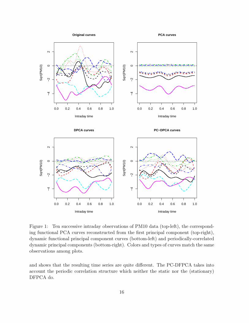
For the sake of comparison and discussion, we focus only on the first principal compo-

nent, which already explains 73% of variability in the static FPCA, 80% of variability in

the DFPCA and 88% of variability in the PC-DFPCA procedure. Curves corresponding

to the components obtained through each of these methods are presented in Figure 1. As

the percentages above suggest, there is a clear progression in the quality of the approxi-

mation using just one component. This is an important finding because the purpose of the

principal component analysis of any type is to reduce the dimension of the data using the

smallest possible number of projections without sacrificing the quality of approximation.

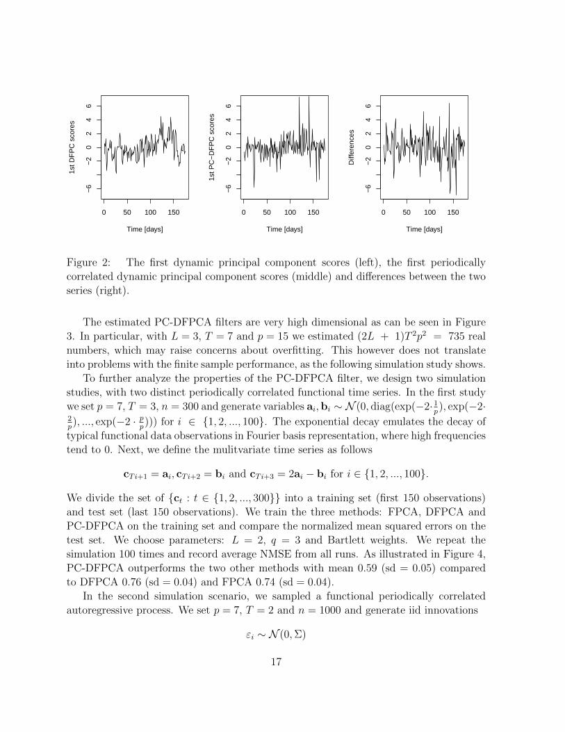
Hormann et al. (2015) observed that, for this particular dataset, the sequences of

scores of the DFPC’s and the static FPC’s were almost identical. This is no longer the

case if the PC-DFPC’s are used. Figure 2 compares the DFPC and the PC-DFPC scores

15

0.0 0.2 0.4 0.6 0.8 1.0

−4

−2

02

Intraday time

Sqr

t(P

M10

)

Original curves

0.0 0.2 0.4 0.6 0.8 1.0

−4

−2

02

Intraday time

Sqr

t(P

M10

)

PCA curves

0.0 0.2 0.4 0.6 0.8 1.0

−4

−2

02

Intraday time

Sqr

t(P

M10

)

DPCA curves

0.0 0.2 0.4 0.6 0.8 1.0

−4

−2

02

Intraday time

Sqr

t(P

M10

)

PC−DPCA curves

Figure 1: Ten successive intraday observations of PM10 data (top-left), the correspond-

ing functional PCA curves reconstructed from the first principal component (top-right),

dynamic functional principal component curves (bottom-left) and periodically-correlated

dynamic principal components (bottom-right). Colors and types of curves match the same

observations among plots.

and shows that the resulting time series are quite different. The PC-DFPCA takes into

account the periodic correlation structure which neither the static nor the (stationary)

DFPCA do.

16

0 50 100 150

−6

−2

02

46

Time [days]

1st D

FP

C s

core

s

0 50 100 150

−6

−2

02

46

Time [days]

1st P

C−

DF

PC

sco

res

0 50 100 150

−6

−2

02

46

Time [days]

Diff

eren

ces

Figure 2: The first dynamic principal component scores (left), the first periodically

correlated dynamic principal component scores (middle) and differences between the two

series (right).

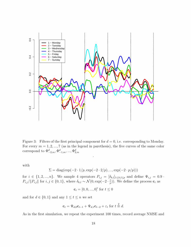
The estimated PC-DFPCA filters are very high dimensional as can be seen in Figure

3. In particular, with L = 3, T = 7 and p = 15 we estimated (2L + 1)T 2p2 = 735 real

numbers, which may raise concerns about overfitting. This however does not translate

into problems with the finite sample performance, as the following simulation study shows.

To further analyze the properties of the PC-DFPCA filter, we design two simulation

studies, with two distinct periodically correlated functional time series. In the first study

we set p = 7, T = 3, n = 300 and generate variables ai,bi ∼ N (0, diag(exp(−2·1p), exp(−2·

2p), ..., exp(−2 · p

p))) for i ∈ 1, 2, ..., 100. The exponential decay emulates the decay of

typical functional data observations in Fourier basis representation, where high frequencies

tend to 0. Next, we define the mulitvariate time series as follows

cT i+1 = ai, cT i+2 = bi and cTi+3 = 2ai − bi for i ∈ 1, 2, ..., 100.

We divide the set of ct : t ∈ 1, 2, ..., 300 into a training set (first 150 observations)

and test set (last 150 observations). We train the three methods: FPCA, DFPCA and

PC-DFPCA on the training set and compare the normalized mean squared errors on the

test set. We choose parameters: L = 2, q = 3 and Bartlett weights. We repeat the

simulation 100 times and record average NMSE from all runs. As illustrated in Figure 4,

PC-DFPCA outperforms the two other methods with mean 0.59 (sd = 0.05) compared

to DFPCA 0.76 (sd = 0.04) and FPCA 0.74 (sd = 0.04).

In the second simulation scenario, we sampled a functional periodically correlated

autoregressive process. We set p = 7, T = 2 and n = 1000 and generate iid innovations

εi ∼ N (0,Σ)

17

−0.

20.

00.

20.

40.

6

1 − Monday2 − Tuesday3 − Wednesday4 − Thursday5 − Friday6 − Saturday7 − Sunday

Figure 3: Filters of the first principal component for d = 0, i.e. corresponding to Monday.

For every m = 1, 2, ..., 7 (as in the legend in parethesis), the five curves of the same color

correspond to Φd−2,m,Φ

d−1,m, ...,Φ

d2,m

.

with

Σ = diag(exp(−2 · 1/p, exp(−2 · 2/p), ..., exp(−2 · p/p)))

for i ∈ 1, 2, ..., n. We sample 4 operators Pi,j = [δk,l]1≤k,l≤p and define Ψi,j = 0.9 ·Pi,j/‖Pi,j‖ for i, j ∈ 0, 1, where δk,l ∼ N (0, exp(−2 · l

p)). We define the process ct as

ct = [0, 0, ..., 0]′ for t ≤ 0

and for d ∈ 0, 1 and any 1 ≤ t ≤ n we set

ct = Ψd,0ct−1 + Ψd,1ct−2 + εt for t2≡ d.

As in the first simulation, we repeat the experiment 100 times, record average NMSE and

18

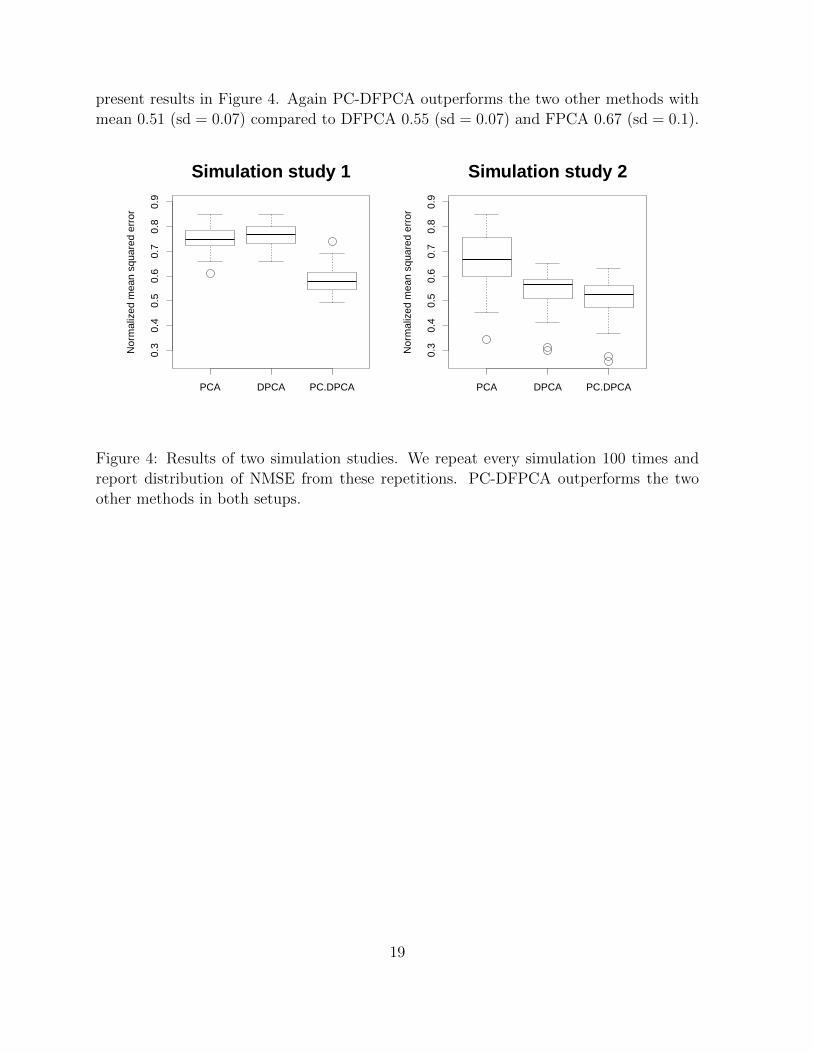
present results in Figure 4. Again PC-DFPCA outperforms the two other methods with

mean 0.51 (sd = 0.07) compared to DFPCA 0.55 (sd = 0.07) and FPCA 0.67 (sd = 0.1).

PCA DPCA PC.DPCA

0.3

0.4

0.5

0.6

0.7

0.8

0.9

Simulation study 1

Nor

mal

ized

mea

n sq

uare

d er

ror

PCA DPCA PC.DPCA

0.3

0.4

0.5

0.6

0.7

0.8

0.9

Simulation study 2

Nor

mal

ized

mea

n sq

uare

d er

ror

Figure 4: Results of two simulation studies. We repeat every simulation 100 times and

report distribution of NMSE from these repetitions. PC-DFPCA outperforms the two

other methods in both setups.

19

6 Proofs of the results of Section 3

To explain the essence and technique of the proofs, we consider the special case of T = 2.

The arguments for general T proceed analogously, merely with a more heavy and less

explicit notation, which may obscure the essential arguments.

Proof of Theorem 3.1: To establish the mean square convergence of the series∑l∈Z Ψt

l

(X(t−l)

), let Sn,t be its partial sum, i.e. Sn,t =

∑−n≤l≤n Ψt

l

(X(t−l)

), for each

positive integer n. Then for m < n we have,

E ‖Sn,t − Sm,t‖2Cp =∑

m<|l|,|k|≤n

E⟨Ψtl

(X(t−l)

),Ψt

k

(X(t−k)

)⟩Cp

≤∑

m<|l|,|k|≤n

E(∥∥Ψt

l

(X(t−l)

)∥∥Cp∥∥Ψt

k

(X(t−k)

)∥∥Cp)

≤∑

m<|l|,|k|≤n

∥∥Ψtl

∥∥L

∥∥Ψtk

∥∥LE

(∥∥X(t−l)∥∥∥∥X(t−k)

∥∥)≤

∑m<|l|,|k|≤n

∥∥Ψtl

∥∥L

∥∥Ψtk

∥∥L

(E∥∥X(t−l)

∥∥2E ∥∥X(t−k)∥∥2) 1

2

≤ M∑|l|>m

∑|k|>m

∥∥Ψtl

∥∥L

∥∥Ψtk

∥∥L for some M ∈ R+

≤ M

∑|l|>m

∥∥Ψtl

∥∥L

2

.(6.1)

Summability condition (2.5) implies that (6.1) tends to zero, as n and m tend to infinity.

Therefore, Sn,t, n ∈ Z+ forms a Cauchy sequence in L2 (Cp,Ω), for each t, which implies

the desired mean square convergence. According to the representation of the filtered

process Y at time t i.e.,

Yt =∑l∈Z

Ψ0l

(X(t−l)

)=

∑l∈Z

Ψ02l

(X(t−2l)

)+∑l∈Z

Ψ02l−1

(X(t−2l+1)

), t

2≡ 0

Yt =∑l∈Z

Ψ1l

(X(t−l)

)=

∑l∈Z

Ψ12l

(X(t−2l)

)+∑l∈Z

Ψ12l+1

(X(t−2l−1)

), t

2≡ 1,

20

for each h ∈ Z we have

Cov (Y2h,Y0) = limn→∞

∑|k|≤n

∑|l|≤n

Cov(Ψ0k

(X(2h−k)

),Ψ0

l

(X(0−l)

))=

∑k∈Z

∑l∈Z

Ψ02kCov

(X(2h−2k), X−2l

) (Ψ0

2l

)∗+∑k∈Z

∑l∈Z

Ψ02kCov

(X(2h−2k), X−2l+1

) (Ψ0

2l−1)∗

+∑k∈Z

∑l∈Z

Ψ02k−1Cov

(X(2h−2k+1), X−2l

) (Ψ0

2l

)∗+∑k∈Z

∑l∈Z

Ψ02k−1Cov

(X(2h−2k+1), X−2l+1

) (Ψ0

2l−1)∗.

Consequently,

FYθ,(0,0) =

1

2π

∑h∈Z

Cov (Y2h,Y0) e−ihθ

=1

2π

∑h∈Z

∑k∈Z

∑l∈Z

Ψ02kCov

(X(2h−2k), X−2l

) (Ψ0

2l

)∗e−ihθ

+1

2π

∑h∈Z

∑k∈Z

∑l∈Z

Ψ02kCov

(X(2h−2k), X−2l+1

) (Ψ0

2l−1)∗e−ihθ

+1

2π

∑h∈Z

∑k∈Z

∑l∈Z

Ψ02k−1Cov

(X(2h−2k+1), X−2l

) (Ψ0

2l

)∗e−ihθ

+1

2π

∑h∈Z

∑k∈Z

∑l∈Z

Ψ02k−1Cov

(X(2h−2k+1), X−2l+1

) (Ψ0

2l−1)∗e−ihθ,

which leads

FYθ,(0,0) =

1

2π

∑k∈Z

∑l∈Z

∑h∈Z

Ψ02kCov

(X(2h−2k+2l), X0

) (Ψ0

2l

)∗e−i(h−k+l)θeilθe−ikθ

+1

2π

∑k∈Z

∑l∈Z

∑h∈Z

Ψ02kCov

(X(2h−2k+2l), X1

) (Ψ0

2l−1)∗e−i(h−k+l)θeilθe−ikθ

+1

2π

∑k∈Z

∑l∈Z

∑h∈Z

Ψ02k−1Cov

(X(2h−2k+2l+1), X0

) (Ψ0

2l

)∗e−i(h−k+l)θeilθe−ikθ

+1

2π

∑k∈Z

∑l∈Z

∑h∈Z

Ψ02k−1Cov

(X(2h−2k+2l+1), X1

) (Ψ0

2l−1)∗e−i(h−k+l)θeilθe−ikθ,

21

=∑k∈Z

∑l∈Z

Ψ02kFXθ,(0,0)

(Ψ0

2l

)∗eilθe−ikθ

+∑k∈Z

∑l∈Z

Ψ02kFXθ,(0,1)

(Ψ0

2l−1)∗eilθe−ikθ

+∑k∈Z

∑l∈Z

Ψ02k−1FXθ,(1,0)

(Ψ0

2l

)∗eilθe−ikθ

+∑k∈Z

∑l∈Z

Ψ02k−1FXθ,(1,1)

(Ψ0

2l−1)∗eilθe−ikθ

= : Ψ0θ,0FXθ,(0,0)

(Ψ0θ,0

)∗+Ψ0

θ,0FXθ,(0,1)(Ψ0θ,−1)∗

+Ψ0θ,−1FXθ,(1,0)

(Ψ0θ,0

)∗+Ψ0

θ,−1FXθ,(1,1)(Ψ0θ,−1)∗.

The operator FYθ,(0,0) from Cp to Cp has the following matrix form(⟨(

FXθ,(0,0))∗ (

Ψ0θ,0,r

),Ψ0

θ,0,q

⟩H

)p×p

+(⟨(FXθ,(0,1)

)∗ (Ψ0θ,0,r

),Ψ0

θ,−1,q⟩H

)p×p

+(⟨(FXθ,(1,0)

)∗ (Ψ0θ,−1,r

),Ψ0

θ,0,q

⟩H

)p×p

+(⟨(FXθ,(1,1)

)∗ (Ψ0θ,−1,r

),Ψ0

θ,−1,q⟩H

)p×p

,

Finally,

FYθ,(0,0) =

⟨ (FXθ,(0,0)

)∗ (FXθ,(1,0)

)∗(FXθ,(0,1)

)∗ (FXθ,(1,1)

)∗( Ψ0

θ,0,r

Ψ0θ,−1,r

),

(Ψ0θ,0,q

Ψ0θ,−1,q

)⟩H2

=

⟨(FXθ,(0,0) FXθ,(0,1)FXθ,(1,0) FXθ,(1,1)

)(Ψ0θ,0,r

Ψ0θ,−1,r

),

(Ψ0θ,0,q

Ψ0θ,−1,q

)⟩H2

.

Using similar arguments leads to the following representations for FYθ,(1,0), FY

θ,(0,1), and

FYθ,(1,1).

FYθ,(1,0) =

⟨(FXθ,(0,0) FXθ,(0,1)FXθ,(1,0) FXθ,(1,1)

)(Ψ1θ,1,r

Ψ1θ,0,r

),

(Ψ0θ,0,q

Ψ0θ,−1,q

)⟩H2

FYθ,(0,1) =

⟨(FXθ,(0,0) FXθ,(0,1)FXθ,(1,0) FXθ,(1,1)

)(Ψ0θ,0,r

Ψ0θ,−1,r

),

(Ψ1θ,1,q

Ψ1θ,0,q

)⟩H2

22

FYθ,(1,1) =

⟨(FXθ,(0,0) FXθ,(0,1)FXθ,(1,0) FXθ,(1,1)

)(Ψ1θ,1,r

Ψ1θ,0,r

),

(Ψ1θ,1,q

Ψ1θ,0,q

)⟩H2

.

Note that the 2-periodic behavior of the covariance operators of the filtered process Y is

an implicit result of the above argument, which completes the proof of Theorem 3.1 for

the special case T = 2. The general case is similar.

Proof of Proposition 3.1: To establish part (a), consider the eigenvalue decomposi-

tion (3.4). We then have

λθ,mϕθ,m =

(FXθ,(0,0) FXθ,(0,1)FXθ,(1,0) FXθ,(1,1)

)(ϕθ,m)

=

(FXθ,(0,0) FXθ,(0,1)FXθ,(1,0) FXθ,(1,1)

)(ϕθ,m,1ϕθ,m,2

)

=

(FXθ,(0,0) (ϕθ,m,1) + FXθ,(0,1) (ϕθ,m,2)

FXθ,(1,0) (ϕθ,m,1) + FXθ,(1,1) (ϕθ,m,2)

)

=1

2π

∑h∈Z

(E[〈ϕθ,m,1, X0〉H + 〈ϕθ,m,2, X1〉H

]X2h

E[〈ϕθ,m,1, X0〉H + 〈ϕθ,m,2, X1〉H

]X2h+1

)e−ihθ.

Consequently,

λθ,mϕθ,m =1

2π

∑h∈Z

E[〈ϕθ,m,1, X0〉H + 〈ϕθ,m,2, X1〉H

]X2h

E[〈ϕθ,m,1, X0〉H + 〈ϕθ,m,2, X1〉H

]X2h+1

e+ihθ

1

2π

∑h∈Z

(E[⟨ϕθ,m,1, X0

⟩H +

⟨ϕθ,m,2, X1

⟩H

]X2h

E[⟨ϕθ,m,1, X0

⟩H +

⟨ϕθ,m,2, X1

⟩H

]X2h+1

)e+ihθ

=

(FX−θ,(0,0) FX−θ,(0,1)FX−θ,(1,0) FX−θ,(1,1)

)(ϕθ,m

).

Hence λθ,m and ϕθ,m are an eigenvalue/eigenfunction pair of

(FX−θ,(0,0) FX−θ,(0,1)FX−θ,(1,0) FX−θ,(1,1)

). Now,

use (3.8) to obtain Φtl,m = Φ

t

l,m, which implies that the DFPC scores Yt,m satisfy

Yt,m =∑l∈Z

⟨Xt−l,Φ

tl,m

⟩H =

∑l∈Z

⟨X t−l,Φ

t

l,m

⟩H

=∑l∈Z

⟨Xt−l,Φt

l,m

⟩H = Y t,m,

and so are real for each t and m.

23

For part (b), first we define Yt,m,n :=∑n

l=−n⟨Xt−l,Φ

tl,m

⟩. Then we use a similar

argument as in the proof of Theorem 3.1 to show that Yt,m,n is converges in mean-square

to Yt,m =∑

l∈Z⟨Xt−l,Φ

tl,m

⟩. Hence

‖E (Yt,m,n ⊗ Yt,m,n)− E (Yt,m ⊗ Yt,m)‖S −→ 0, as n −→∞,

or equevalently, ∣∣E ‖Yt,m,n‖2C − E ‖Yt,m‖2C∣∣ −→ 0, as n −→∞.

Consequently, for t2≡ 0, we have

E ‖Yt,m‖2C = limn→∞

EYt,m,nY t,m,n = limn→∞

∑|k|≤n

∑|l|≤n

E⟨Xt−l,Φ

0l,m

⟩ ⟨Φ0k,m, Xt−k

⟩=

∑k∈Z

∑l∈Z

E⟨Xt−2l,Φ

02l,m

⟩ ⟨Φ0

2k,m, Xt−2k⟩

+∑k∈Z

∑l∈Z

E⟨Xt−2l,Φ

02l,m

⟩ ⟨Φ0

2k−1,m, Xt−2k+1

⟩+∑k∈Z

∑l∈Z

E⟨Xt−2l+1,Φ

02l−1,m

⟩ ⟨Φ0

2k,m, Xt−2k⟩

+∑k∈Z

∑l∈Z

E⟨Xt−2l+1,Φ

02l−1,m

⟩ ⟨Φ0

2k−1,m, Xt−2k+1

⟩=

∑k∈Z

∑l∈Z

⟨CXk−l,(0,0)

(Φ0

2k,m

),Φ0

2l,m

⟩H

+∑k∈Z

∑l∈Z

⟨CXk−l,(0,1)

(Φ0

2k−1,m),Φ0

2l,m

⟩H

+∑k∈Z

∑l∈Z

⟨CXk−l,(1,0)

(Φ0

2k,m

),Φ0

2l−1,m⟩H

+∑k∈Z

∑l∈Z

⟨CXk−l,(1,1)

(Φ0

2k−1,m),Φ0

2l−1,m⟩H.

That is the desired result for the case t2≡ 0. The case t

2≡ 1 is handled in a similar way.

Part (c) is a direct result of Theorem 3.1, so we can proceed to the proof of part (d).

Considering part (c) and using the results of Proposition 3 of Hormann et al. (2015) lead

to the desired result for 2n in place of n.

limn→∞

1

2nVar (Y1 + · · ·+ Y2n)

= limn→∞

1

2n[Var (Y1 + Y3 + · · ·+ Y2n−1) + Var (Y2 + Y4 + · · ·+ Y2n)]

=2π

2[diag (λ0,1, . . . , λ0,p) + diag (λ0,p+1, . . . , λ0,2p)] ,

and similarly for 2n+ 1 in place of 2n. This completes the proof.

24

Proofs of Theorems 3.2 and 3.3: Consider the H2-valued mean zero stationary

process X =X t =

(X2t X2t+1

)′, t ∈ Z

and the filter Ψl, l ∈ Z with the following

matrix form

Ψl =

(Ψ0

2l Ψ02l−1

Ψ12l+1 Ψ1

2l

): H2−→

((Cp)2

)C2p,

where

Ψtl : H −→Cp

Ψtl : h 7−→

(⟨h,Ψt

l,1

⟩, . . . ,

⟨h,Ψt

l,p

⟩)′, t = 0, 1, l ∈ Z.

Similarly, define the sequence of operators Υl, l ∈ Z with

Υ−l =

(Υ0

2l Υ02l+1

Υ12l−1 Υ1

2l

):((Cp)2

)C2p−→ H2,

where

Υtl : Cp−→ H

Υtl : y 7−→

p∑m=1

ymΥtl,m, t = 0, 1, l ∈ Z.

Therefore,

Υ (B) Ψ (B)X t =

p∑m=1

(X2t,m

X2t+1,m

).

On the other hand, there exist elements ψlq =(ψlq,1 ψlq,2

)′and υlq =

(υlq,1 υlq,2

)′,

q = 1, . . . , 2p, in H2, such that

Ψl (h) = Ψl

((h1, h2)

′) =(⟨h, ψl1

⟩H2 , . . . ,

⟨h, ψl2p

⟩H2

)′=

(⟨h1, ψ

l1,1

⟩+⟨h2, ψ

l1,2

⟩, . . . ,

⟨h1, ψ

l2p,1

⟩+⟨h2, ψ

l2p,2

⟩)′, ∀h1, h2 ∈ H,

and

Υ−l (y) = Υ−l((y1, y2)

′)=

p∑m=1

y1,mυlm +

p∑m=1

y2,mυlm+p, ∀y1, y2 ∈ Cp.

Simple calculations lead to the following relations, valid for m = 1, . . . , p, which play a

crucial role in the remainder of the proof:

ψlm =

(ψlm,1ψlm,2

)=

(Ψ0

2l,m

Ψ02l−1,m

), ψlm+p =

(ψlm+p,1

ψlm+p,2

)=

(Ψ1

2l+1,m

Ψ12l,m

),

25

υlm =

(υlm,1υlm,2

)=

(Υ0

2l,m

Υ12l−1,m

), υlm+p =

(υlm+p,1

υlm+p,2

)=

(Υ0

2l+1,m

Υ12l,m

).

According to Hormann et al. (2015), we can minimize

E ‖X t −Υ (B) Ψ (B) (X t)‖2H2

by choosing υθ,m =∑

l∈Z υlme

ilθ = ψθ,m =∑

l∈Z ψlme

ilθ as the m-th eigenfunctions of the

spectral density operator FXθ of the process X. Note that FXθ is nothing other than

FXθ (h) = FXθ((

h1h2

))=

(FXθ,(0,0) FXθ,(0,1)FXθ,(1,0) FXθ,(1,1)

)(h1h2

), ∀h1, h2 ∈ H.

This completes the proof.

Proof of Theorem 3.4: We will use the continuity of each function λ·,m. This is a

direct consequence of Proposition 7 of Hormann et al. (2015). As in the proof of Theorem

3 of Hormann et al. (2015), we show that E∣∣∣Yt,m − Yt.m∣∣∣ −→ 0. For a fixed L and t

2≡ 0

we have,

E∣∣∣Yt,m − Yt.m∣∣∣ = E

∣∣∣∣∣∣2L∑

l=−2L−1

⟨Xt−l,Φ

0l,m − Φ0

l,m

⟩H

+∑

l /∈[−2L−1,2L]

⟨Xt−l,Φ

0l,m

⟩H

∣∣∣∣∣∣≤ E

∣∣∣∣∣2L∑

l=−2L−1

⟨Xt−l,Φ

0l,m − Φ0

l,m

⟩H

∣∣∣∣∣+ E

∣∣∣∣∣∣∑

l /∈[−2L−1,2L]

⟨Xt−l,Φ

0l,m

⟩H

∣∣∣∣∣∣(6.2)

= E

∣∣∣∣∣L∑

l=−L

⟨Xt−2l,Φ

02l,m − Φ0

2l,m

⟩H

+L∑

l=−L

⟨Xt−2l+1,Φ

02l−1,m − Φ0

2l−1,m

⟩H

∣∣∣∣∣+E

∣∣∣∣∣∣∑|l|>L

⟨Xt−2l,Φ

02l,m

⟩H +

∑|l|>L

⟨Xt−2l+1,Φ

02l−1,m

⟩H

∣∣∣∣∣∣ .Thus, it is enough to show that each of the terms appearing in (6.2) converges to zero in

26

probability. The first term can be bounded as follows:

E

∣∣∣∣∣2L∑

l=−2L−1

⟨Xt−l,Φ

0l,m − Φ0

l,m

⟩H

∣∣∣∣∣≤ E

2L∑l=−2L−1

‖Xt−l‖∥∥∥Φ0

l,m − Φ0l,m

∥∥∥= E

L∑l=−L

‖Xt−2l‖∥∥∥Φ0

2l,m − Φ02l,m

∥∥∥+E

L∑l=−L

‖Xt−2l+1‖∥∥∥Φ0

2l−1,m − Φ02l−1,m

∥∥∥≤ E

L∑l=−L

‖Xt−2l‖(∥∥∥Φ0

2l,m − Φ02l,m

∥∥∥2 +∥∥∥Φ0

2l−1,m − Φ02l−1,m

∥∥∥2) 12

+EL∑

l=−L

‖Xt−2l+1‖(∥∥∥Φ0

2l,m − Φ02l,m

∥∥∥2 +∥∥∥Φ0

2l−1,m − Φ02l−1,m

∥∥∥2) 12

≤ 2EL∑

l=−L

∥∥∥X( t2−l)

∥∥∥H2

∥∥∥∥( Φ02l,m Φ0

2l−1,m)′ − ( Φ0

2l,m Φ02l−1,m

)′∥∥∥∥H2

.(6.3)

Next, we use (3.8) to obtain

2π

∥∥∥∥( Φ02l,m Φ0

2l−1,m)′ − ( Φ0

2l,m Φ02l−1,m

)′∥∥∥∥H2

=

∥∥∥∥∫ π

−π(ϕθ,m − ϕθ,m) e−ilθdθ

∥∥∥∥H2

≤∫ π

−π‖ϕθ,m − ϕθ,m‖H2 dθ

=

∫ π

−π‖ϕθ,m − (1− cθ,m + cθ,m) ϕθ,m‖H2 dθ

≤∫ π

−π‖ϕθ,m − cθ,mϕθ,m‖H2 dθ +

∫ π

−π‖(1− cθ,m) ϕθ,m‖H2 dθ

=

∫ π

−π‖ϕθ,m − cθ,mϕθ,m‖H2 dθ +

∫ π

−π|1− cθ,m| dθ

= : Q1 +Q2,

where cθ,m :=〈ϕθ,m,ϕθ,m〉H2

|〈ϕθ,m,ϕθ,m〉H2|, m = 1, . . . , p. According to Lemma 3.2 of Hormann and

27

Kokoszka (2010) we have the following upper bound for Q1:

Q1 ≤∫ π

−π

2√

2

αθ,m

∥∥∥FXθ − FXθ ∥∥∥L ∧ 2dθ

≤∫ π

−π

2√

2

αθ,m

∥∥∥FXθ − FXθ ∥∥∥S ∧ 2dθ.(6.4)

By Condition 3.2 there is a finite subset θ1, . . . , θK of (−π, π] for which αθ1,m = · · · =

αθK ,m = 0. DefineA (m, ε) :=⋃Kj=1 [θj − ε, θj + ε] andM−1

ε := min αθ,m : θ ∈ [−π, π] \ A (m, ε).Therefore the upper bound (6.4) satisfies∫ π

−π

2√

2

αθ,m

∥∥∥FXθ − FXθ ∥∥∥S ∧ 2dθ ≤ 4Kε+ 8M2ε

∫ π

−π

2√

2

αθ,m

∥∥∥FXθ − FXθ ∥∥∥S dθ: = Bn,ε.

Now, use the countinuty of λ·,m and Condition 3.1 and choose ε > 0, small enough to

conclude Bn,ε tends to zero in probability. Thus,

(6.5)

∫ π

−π|〈ϕθ,m, ω〉 − c (θ) 〈ϕθ,m, ω〉| dθ −→ 0 in probability.

By applying similar argument as in the proof of Theorem 3 of Hormann et al. (2015), we

also conclude that Q2 tends to zero in probability. Remark 2.1 entails

E

∣∣∣∣∣2L∑

l=−2L−1

⟨Xt−l,Φ

0l,m − Φ0

l,m

⟩H

∣∣∣∣∣≤ E

2L∑l=−2L−1

‖Xt−l‖H∥∥∥Φ0

l,m − Φ0l,m

∥∥∥H

≤ Q1 +Q2

2π

2L∑l=−2L+1

E ‖Xt−l‖H

≤ oP (1)

∑2Ll=−2L+1E ‖Xt−l‖H

L

≤ oP (1)

∑2Ll=−2L+1

(E ‖Xt−l‖2H

) 12

L

≤ oP (1)(4L+ 2)

(max0≤t≤T−1

(E ‖Xt‖2

)) 12

L−→ 0.

It remains to show that E∣∣∣∑|l|>L ⟨Xt−2l,Φ

02l,m

⟩H +

∑|l|>L

⟨Xt−2l+1,Φ

02l−1,m

⟩H

∣∣∣2 tends to

28

zero.

E

⟨∑|l|>L

⟨Xt−2l,Φ

02l,m

⟩H +

⟨Xt−2l+1,Φ

02l−1,m

⟩H ,∑|k|>L

⟨Xt−2k,Φ

02k,m

⟩H +

⟨Xt−2k+1,Φ

02k−1,m

⟩H

⟩C

=∑|l|>L

∑|k|>L

⟨E (Xt−2l ⊗Xt−2k) Φ0

2k,m,Φ02l,m

⟩H

+∑|l|>L

∑|k|>L

⟨E (Xt−2l ⊗Xt−2k+1) Φ0

2k−1,m,Φ02l,m

⟩H

+∑|l|>L

∑|k|>L

⟨E (Xt−2l+1 ⊗Xt−2k) Φ0

2k,m,Φ02l−1,m

⟩H

+∑|l|>L

∑|k|>L

⟨E (Xt−2l+1 ⊗Xt−2k+1) Φ0

2k−1,m,Φ02l−1,m

⟩H

Cauchy-Schwartz inequality entails

E

∣∣∣∣∣∣∑|l|>L

⟨Xt−2l,Φ

02l,m

⟩H +

∑|l|>L

⟨Xt−2l+1,Φ

02l−1,m

⟩H

∣∣∣∣∣∣2

≤∑|k|>L

∑|l|>L

∥∥CXk−l,(0,0)

∥∥L

∥∥Φ02k,m

∥∥∥∥Φ02l,m

∥∥+∑|k|>L

∑|l|>L

∥∥CXk−l,(0,1)

∥∥L

∥∥Φ02k−1,m

∥∥∥∥Φ02l,m

∥∥+∑|k|>L

∑|l|>L

∥∥CXk−l,(1,0)

∥∥L

∥∥Φ02k,m

∥∥∥∥Φ02l−1,m

∥∥+∑|k|>L

∑|l|>L

∥∥CXk−l,(1,1)

∥∥L

∥∥Φ02k−1,m

∥∥∥∥Φ02l−1,m

∥∥=

∑h∈Z

∑k∈Z

∥∥CXh,(0,0)

∥∥L

∥∥Φ02k,m

∥∥∥∥Φ02(k−h),m

∥∥ I |k| > L I |k − h| > L

+∑h∈Z

∑k∈Z

∥∥CXh,(0,1)

∥∥L

∥∥Φ02k−1,m

∥∥∥∥Φ02(k−h),m

∥∥ I |k| > L I |k − h| > L

+∑h∈Z

∑k∈Z

∥∥CXh,(1,0)

∥∥L

∥∥Φ02k,m

∥∥∥∥Φ02(k−h)−1,m

∥∥ I |k| > L I |k − h| > L

+∑h∈Z

∑k∈Z

∥∥CXh,(1,1)

∥∥L

∥∥Φ02k−1,m

∥∥∥∥Φ02(k−h)−1,m

∥∥ I |k| > L I |k − h| > L

29

≤∑h∈Z

∥∥CXh,(0,0)

∥∥L

(∑k∈Z

∥∥Φ02k,m

∥∥2 I |k| > L

) 12(∑k∈Z

∥∥Φ02k,m

∥∥2) 12

+∑h∈Z

∥∥CXh,(0,1)

∥∥L

(∑k∈Z

∥∥Φ02k−1,m

∥∥2 I |k| > L

) 12(∑k∈Z

∥∥Φ02k,m

∥∥2) 12

+∑h∈Z

∥∥CXh,(1,0)

∥∥L

(∑k∈Z

∥∥Φ02k,m

∥∥2 I |k| > L

) 12(∑k∈Z

∥∥Φ02k−1,m

∥∥2) 12

+∑h∈Z

∥∥CXh,(1,1)

∥∥L

(∑k∈Z

∥∥Φ02k−1,m

∥∥2 I |k| > L

) 12(∑k∈Z

∥∥Φ02k−1,m

∥∥2) 12

,

which obviously tends to zero as n tends to infinity. Using a similar argument for case

t2≡ 1 completes the proof.

References

Anderson, P. L. and Meerschaert, M. M. (1997). Periodic moving averages of random variableswith regularly varying tails. Annals of Statistics, 24, 771–785.

Aue, A., Dubart-Norinho, D. and Hormann, S. (2015). On the prediction of stationary functionaltime series. Journal of the American Statistical Association, 110, 378–392.

Brillinger, D. R. (1975). Time Series: Data Analysis and Theory. Holt, New York.

Fisher, R. A. (1929). Tests of significance in harmonic analysis. Proceedings of the Royal Society(A), 125, 54–59.

Ghanbarzadeh, M. and Aminghafari, M. (2016). A wavelet characterization of continuous-time periodically correlated processes with application to simulation. Journal of Time SeriesAnalysis, 37, 741–762.

Gromenko, O., Kokoszka, P. and Reimherr, M. (2016). Detection of change in the spatiotemporalmean function. Journal of the Royal Statistical Society (B), 00, 00–00; Forthcoming.

Hays, S., Shen, H. and Huang, J. Z. (2012). Functional dynamic factor models with applicationto yield curve forecasting. The Annals of Applied Statistics, 6, 870–894.

Hormann, S., Kidzinski, L. and Hallin, M. (2015). Dynamic functional principal components.Journal of the Royal Statistical Society (B), 77, 319–348.

Hormann, S. and Kokoszka, P. (2010). Weakly dependent functional data. The Annals ofStatistics, 38, 1845–1884.

Hormann, S., Kokoszka, P. and Nisol, G. (2016). Detection of periodicity in functional timeseries. Technical Report. Universite libre de Bruxelles.

Horvath, L. and Kokoszka, P. (2012). Inference for Functional Data with Applications. Springer.

30

Horvath, L., Kokoszka, P. and Rice, G. (2014). Testing stationarity of functional time series.Journal of Econometrics, 179, 66–82.

Hurd, H. L. (1989). Nonparametric time series analysis for periodically correlated processes.IEEE Trans. Inform. Theory, 35, 350–359.

Hurd, H. L. and Miamee, A. (2007). Periodically Correlated Random Sequences. Wiley.

Javorskyj, I., Leskow, J., Kravets, I., Isayev, I. and Gajecka, E. (2012). Linear filtrationmethods for statistical analysis of periodically correlated random processes-part I: Coherentand component methods and their generalization. Signal Processing, 92, 1559 – 1566.

Klepsch, J., Kluppelberg, C. and Wei, T. (2017). Prediction of functional ARMA processeswith an application to traffic data. Econometrics and Statistics, 00, 000–000; Forthcoming.

Kokoszka, P. and Reimherr, M. (2017). Introduction to Functional Data Analysis. CRC Press.

Lund, R., Hurd, H., Bloomfield, P. and Smith, R. (1995). Climatological time series withperiodic correlation. Journal of Climate, 8, 410–427.

Panaretos, V. M. and Tavakoli, S. (2013a). Cramer–Karhunen–Loeve representation and har-monic principal component analysis of functional time series. Stochastic Processes and theirApplications, 123, 2779–2807.

Panaretos, V. M. and Tavakoli, S. (2013b). Fourier analysis of stationary time series in functionspace. The Annals of Statistics, 41, 568–603.

Ramsay, J., Hooker, G. and Graves, S. (2009). Functional Data Analysis with R and MATLAB.Springer.

Walker, G. (1914). On the criteria for the reality of relationships or periodicities. Calcutta Ind.Met. Memo, 21, number 9.

Zamani, A., Haghbin, H. and Shishebor, Z. (2016). Some tests for detecting cyclic behavior infunctional time series with application in climate change. Technical report. Shiraz University.

Zhang, X. (2016). White noise testing and model diagnostic checking for functional time series.Journal of Econometrics, 194, 76–95.

31