Pricing Tranched Credit Products with Generalized ... · Pricing Tranched Credit Products with...
44
Pricing Tranched Credit Products with Generalized Multifactor Models M. Moreno J. I. Pe˜ na P. Serrano ∗ October 22, 2007 * We want to thank to A. Novales for his helpful comments. Serrano acknowledges finan- cial support from the Plan Nacional de I+D+I (project BEC2003-02084) and especially to Jose M. Usategui. Pe˜ na thanks financial support from MEC grant SEJ2005-05485. Manuel Moreno is from University of Castilla La-Mancha, Facultad CC. Juridicas y So- ciales, Cobertizo de San Pedro Martir, Dpto Analisis Economico y Finanzas, Toledo, Spain. E-mail: [email protected]. Juan Ignacio Pe˜ na is from University Carlos III, Dpto. Economia de la Empresa, Madrid, Spain. E-mail: [email protected]. Pedro Serrano is from University of Basque Country, Facultad CC. Economicas, Dpto. Fundamentos del Analisis Economico II, Avda. Lehendakari Aguirre, 83, 48015 Bilbao, Spain. E-mail: [email protected]. 1
Transcript of Pricing Tranched Credit Products with Generalized ... · Pricing Tranched Credit Products with...

Pricing Tranched Credit Products with
Generalized Multifactor Models
M. Moreno J. I. Pena P. Serrano ∗
October 22, 2007
∗We want to thank to A. Novales for his helpful comments. Serrano acknowledges finan-cial support from the Plan Nacional de I+D+I (project BEC2003-02084) and especiallyto Jose M. Usategui. Pena thanks financial support from MEC grant SEJ2005-05485.Manuel Moreno is from University of Castilla La-Mancha, Facultad CC. Juridicas y So-ciales, Cobertizo de San Pedro Martir, Dpto Analisis Economico y Finanzas, Toledo, Spain.E-mail: [email protected]. Juan Ignacio Pena is from University Carlos III, Dpto.Economia de la Empresa, Madrid, Spain. E-mail: [email protected]. Pedro Serranois from University of Basque Country, Facultad CC. Economicas, Dpto. Fundamentosdel Analisis Economico II, Avda. Lehendakari Aguirre, 83, 48015 Bilbao, Spain. E-mail:[email protected].
1
Abstract
The market for tranched credit products (CDOs, Itraxx tranches) isone of the fastest growing segments in the credit derivatives industry.However, some assumptions underlying the standard Gaussian one-factor pricing model (homogeneity, single factor, Normality), whichis the pricing standard widely used in the industry, are probably toorestrictive. In this paper we generalize the standard model by meansof a two by two model (two factors and two asset classes). We as-sume two driving factors (business cycle and industry) with indepen-dent t-Student distributions, respectively, and we allow the model todistinguish among portfolio assets classes. In order to illustrate theestimation of the parameters of the model, an empirical applicationwith Moody’s data is also included and potential relationships betweendefault rates and macroeconomic variables are analyzed.
Keywords: Collateral Debt Obligations, Factor Models, Probit-Logit Mod-els
Journal of Economic Literature classification: G13, C35, C51
2

1 Introduction
The market of credit tranched products is one of the fastest growing segmentsin the credit derivative industry. As an example, Tavakoli (2003) reports anincrease in market size from almost $19 billions in 1996, to $200 billions in2001. Recent reports estimate market size to be $20 trillions in 2006.1 Asa result, an increasing attention of the financial sector audience has focusedon the pricing of these new products.
The development of pricing models for multiname derivatives is relativelyrecent. As pointed out by Hull and White (2004), the standard approach onthe credit risk literature tends to subdivide the pricing models for multinamederivatives in two groups: structural models, which are those inspired in Mer-ton’s (1974) model or Black and Cox (1976), or the intensity based approach,like Duffie and Garlenau (2001). Roughly speaking, their differences remainon how the probability of default of a firm is obtained: using their fundamen-tal variables - assets and liabilities - as in the case of the structural models,or using directly market spreads, as in the intensity models approach. Up toa point, the structural based approach has been extensively implemented bythe financial sector, maybe due to the extended use of industrial models likeVasicek (1987) or Creditmetrics model of Gupton, Finger and Bathia (1997).2
However, recent academic literature analyze the prices of CDO tranches us-ing intensity models, as Longstaff and Rajan (2006). We refer to Bieleckiand Rutkowski (2002) for a general presentation of structural and intensitybased models.
This paper presents an extension of the standard Gaussian model of Va-sicek (1991), in line with the structural models literature. Basically, Vasicek’s(1991) model assumes that the value of a firm is explained by the weightedaverage of one common factor for every asset plus an independent idiosyn-cratic factor. By means of linking the realization of one systematic factorto every firm’s values, Vasicek (1991) provides a simple way to reduce thecomplexity of dealing with dependence relationships between firms. Gibson(2004) or Gregory and Laurent (2004, 2005) provide additional insights aboutrisk features of this model.
1See BBA Credit Derivatives Report (2006).2It is worth mentioning that the appearance of techniques within the Structural frame-
work that diminishes the traditional high computing cost of multiname credit derivatives(see Andersen, Sidenius and Basu (2003) or Glasserman and Suchitabandid (2006), amongothers) has contributed to the widely usage of structural models.
3

Our approach relies on the connection between the changes of value of afirm and the sum of two factors: systematic and idiosyncratic. Our approachovercomes the limitations of the standard Gaussian model: the different areasor regions of correlation that could compose a credit portfolio (see Gregoryand Laurent, 2004). This article presents a model that captures some ofthe facts found in real data. Motivated by this fact, this article proposes anextension to the two Gaussian asset classes as in Schonbucher (2003). Ourpaper extends the existing literature in three ways: firstly, the assumption ofasset homogeneity is relaxed by introducing two asset classes. Secondly, weconsider an additional source of systematic risk by including another commonfactor related with industry factors. Finally the normality assumption oncommon factors is relaxed.
This paper is divided as follows: Section 2 presents the model. Section 3studies the sensitivity to correlation and to changes in credit spreads. Sec-tion 4 addresses the econometric modelling. Finally, some conclusions arepresented on section 5.
2 The model
To motivate our model we discuss some empirical features found in CDOdata that are not captured by the standard Gaussian models and propose anextension to the asset class models posited by Schonbucher (2003). Notationis taken from Mardia, Kent and Bibby (1979).
2.1 The standard Gaussian model
The Gaussian model introduced by Vasicek (1991) has become a standardin the industry. Basically, it addresses in a simple and elegant way the keyinput in CDOs price: the correlation in default probabilities between firmsaffects the price of the CDO.
Usually a CDO is based on a large portfolio of firms bonds or CDS.3 LetVn×1 (subscript denotes matrix dimension) be a random vector with meanzero and covariance matrix Σ. As standard notation in multivariate analysis,we will define the p-factor model as
Vn×1 = Λn×pFp×1 + un×1 (1)
3CDO tranches of NYME are composed by 100 firms.
4

where Fp×1 and un×1 are random variables with different distributions.The interpretation of the model (1) is the following:
• The vector Vn×1 represents the value of the assets for each of theindividual n-obligors.
• The vector Fp×1 captures the effect of systematic factors - businesscycle, industry, etc. - that affect to the whole economy.
• By contrast, un×1 represents the idiosyncratic factors that affect eachof the n-companies.
• Finally, Λn×p is called the loading matrix, and determines the correla-tion between each of the n-firms.
By assumption, we have that
E(F) = 0, V ar(F) = I, (2)
E(u) = 0, cov(ui,uj) = 0, i 6= j, (3)
and
cov(F,u) = 0 (4)
where I is the identity matrix.We will also assume that vector un×1 is standardized to have zero mean
and unit variance.Using a simplified form of equation (1), Vasicek (1991) assumes that
firm’s values in the asset pool backing the CDO are affected by the sum oftwo elements: on one hand, a common factor to every firm which representsthe systematic component represented by the factor F ; on the other hand,an idiosyncratic component modelled by a noise εi. Both are assumed to bestandard N(0,1) random variables
Vi = ρi1F1 +√
1 − ρi12εi, with i ≤ n (5)
By means of equation (5) it is possible to capture the correlation betweendifferent firms in a portfolio. As equation (5) reveals, Vasicek (1987) assumes
5

that correlation coefficient is homogeneous for each pair of firms.4 Addition-ally, the simplicity of their assumptions permits a fast computation of CDOprices under this framework.
As an immediate consequence of equation (5), a further step is given bygeneralizing the number of factors that affects firms values. Thus, Lucas,Klaassen, Spreij and Staetmans (2001) consider the following factor model
Vi =
p∑
j=1
ρijFj +
√√√√1 −
p∑
j=1
ρij2ui, with i ≤ n (6)
where Vi represents the value of the i-company, Fj , j = 1, ..., p capture theeffect of p-systematic factors and ui is the idiosyncratic factor associatedto the i-firm. Needless to say, assumptions on the distribution of commonand idiosyncratic factors (F and u, respectively) could be imposed. Hulland White (2004) also includes an extension to many factors, including thet-Student distributed case. Finally, Glasserman and Suchitabandid (2006)implements in a recent paper numerical approximations to deal with thesemultifactor structures within a Gaussian framework.
With the purpose of getting intuition about the behaviour of these dif-ferent models, Figure 1 exhibits the loss distribution generated by three al-ternative models:
• The standard Gaussian model (Vasicek, 1991),
V Gi = ρi1F1 +
√1 − ρi1
2εi, and F1, εi ∼ N (0, 1)
• The one factor double-t model (Hull and White, 2004),
V Si = ρi1F1 +
√1 − ρi1
2εi,
where F1 and εi follows t-Student distributions, with 6 degrees of free-dom.
• The two-factor Gaussian model (Hull and White (2004), or Glassermanand Suchitabandid, 2006),
V DGi = ρi1F1 + ρi2F2 +
√1 − ρi1
2 − ρi22εi
with F1, F2, εi ∼ N (0, 1) and ρ2i1 + ρ2
i2 < 1.
4For a detailed exposition of assumptions in structural models see Bielecki andRutkowski (2002).
6

As we will see later, the loss distribution plays a role crucial in the CDOpricing. Different distributions are computed for a portfolio of 100 firms, withconstant default intensities of 1% per year. Correlation parameters are 0.3for all models, except for two-Gaussian factor, with 0.1 and 0.3. The double-tmodel considers a common and idiosyncratic factors each distributed as t-Student with 6 degrees of freedom. The picture shows that, under the samecorrelation parameters, the standard Gaussian model assigns lower probabil-ity to high losses (see for instance the case of 20 firms) than the double-tmodel. By considering an additional factor, as in the 2-Gaussian case, theprobability of high losses is substantially higher than in previous cases.
[INSERT FIGURE 1 AROUND HERE]
Table 1 presents the spreads (in basis points) of a 5-years CDO portfoliocomposed by 100 firms. The individual default probabilities are constant andfixed at 1%. The recovery rate is 40%, a standard in the market. Finally,the different correlation parameters are displayed in the table. We rememberthat all spreads are obtained considering only one asset class. As Table1 shows, results are consistent with the loss distribution lines presented inFigure 1: the double t-Student distribution gives prices systematically biggerthan those obtained for the standard Gaussian model, keeping constant thecorrelation. In the 2 Gaussian factor model prices, we observe a mixture ofeffects due to different combinations of correlations in the portfolio.
[INSERT TABLE 1 AROUND HERE]
2.2 A 2-by-2 model
Generally, as considered by Schonbucher (2003) or Lando (2004), a creditportfolio is composed by different asset classes or buckets, attending to cri-teria of investment grade, non-investment grade assets or industry, amongothers. The exposure of a credit portfolio to a set of common risk factorscould be significant between groups, but should be homogeneous within them.In line with this, the idea of two groups of assets treated in different ways isa more realistic assumption.
As pointed out by Gregory and Laurent (2004), the one-factor modelimposes a limited correlation structure on the credit portfolio, which is notrealistic. Initially, one can argue that increasing the number of factors could
7

be enough to capture a richer structure of correlation within the portfolio.However, this is not yet consistent with the idea of heterogeneity correlationamong groups, due to the fact that every asset is exposed to the same degreeof correlation. By contrast, a richer correlation structure could be imposedin the portfolio if these two groups are treated in different ways.
To illustrate these ideas, Figure 2 shows the yearly percentage defaultrates for investment and non-investment grades. Rates for investment datahave been multiplied by ten with the intention of clarifying the exposition.Figure 2 reveals that correlation between these two assets groups variesthrough time: periods with high degree of default in non-investment gradeassets do not match with high default rates for investment grade. With refer-ence to this idea, Figure 3 displays the correlation coefficients computed usinga moving window of five years. This also provides some additional insightson the degree of correlation between asset classes: the picture shows how thecorrelation among different groups changes during the sample period, fromnegative correlation (1975, 1977 or 1990), to zero (1993, 1996) or highlypositive (1982, 1995 or 2000). These differences in default rates throughtime could reveal the existence of an idiosyncratic component between assetclasses. This fact could support the idea of modelling in a different way thebehaviour of different assets.
[INSERT FIGURES 2 AND 3 AROUND HERE]
This article considers a family of models that take account the existence ofthese different asset classes or regions, in line with the suggestions of Gregoryand Laurent (2004). We analyze a model in the line of the two assets-twoGaussian factor model of Schonbucher (2004), where no distinction is madebetween the obligors which belongs to the same class. Our model generalizesthat posited by Schonbucher (2004) by considering a t-Student distribution,which assigns a higher probability to high default events. Empirical evidenceseems to go in this direction.5 Our work contributes to the existing literaturein the analysis of these asset class models. To the best of our knowledge, nosimilar studies has been reported yet in this direction.
The model we propose is a two-by-two factor model as follows6
5See, for example, Mashal and Naldi (2002).6For the sake of brevity, we omit the graph of th loss distribution implied by this model.
8

Vi1 = α11F1 + α12F2 + β1ui1
Vi2 = α21F1 + α22F2 + β2ui2 (7)
where
• Vi1, Vi2 (i < n) represents the value of the i-company which belongs tothe different asset class
• Fj, j = 1, 2 captures the effect of systematic factors - business cycle andindustry - with independent t- distributions with nj degrees of freedom,and
• ui1, ui2 are idiosyncratic factors distributed also with ni1, ni2 degreesof freedom, respectively.
Under the assumptions of factor models, Fj are scaled to have variance
1, then α11 = ρ11
√n1−2
n1and so on. Idiosyncratic errors are also scaled, for
instance β1 =√
ni1−2ni1
√1 − α2
11 − α212. Finally, we assume the same default
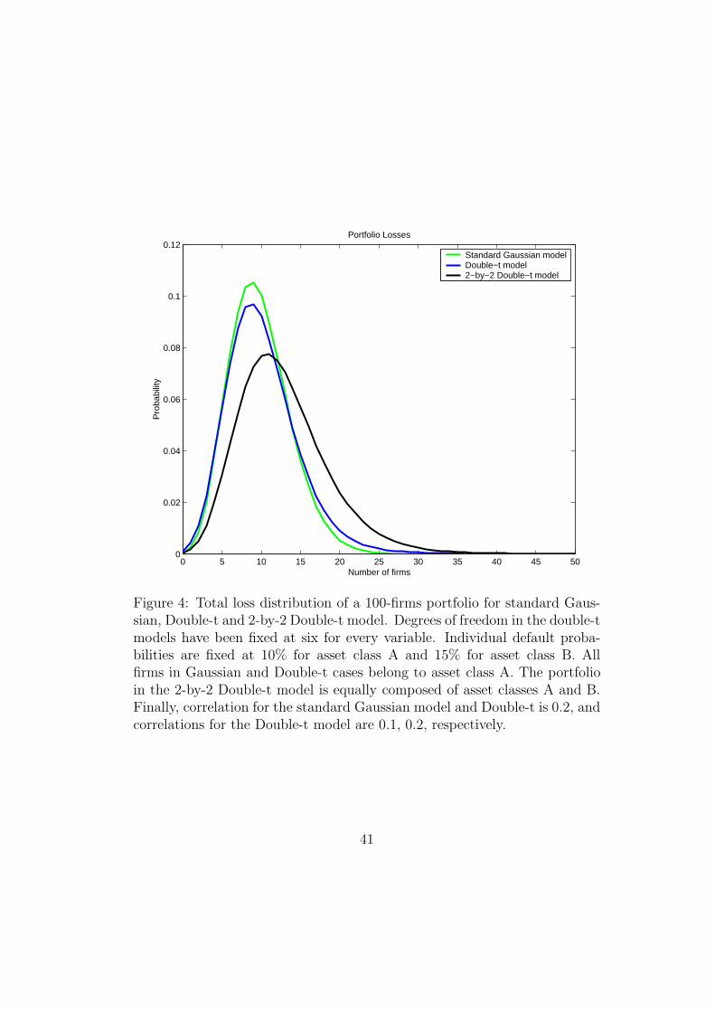
barriers Ki1, Ki2 for the obligors of the same class.Figure 4 displays the simulated distribution for a portfolio of 100 obligors
under the standard Gaussian model of Vasicek (1991), the double-t model ofHull and White (2004) and the 2-by-2 double-t model proposed in equation(7). Risk neutral default intensities have been fixed at 10% for asset classA and 15% for asset class B. We consider homogeneous firms of class A forGaussian and double-t models. The portfolio in the 2-by-2 Double-t modelis equally composed of asset classes A and B. Finally, correlation parametersare 0.2 for the standard Gaussian and double-t models, and 0.1, 0.2 for the2-by-2 double-t model, respectively. As Figure 4 exhibits, the 2-by-2 modelallocates more probability in the tail of the loss distribution than one factormodels, which results in an increasing (decreasing) value for risky (safe)tranches.
[INSERT FIGURE 4 AROUND HERE]
Needless to say that the model could be easily generalized to the case ofm-asset classes, as follows:
9

Vi,m =
p∑
h=1
ρmhFh + ui,m
√√√√1 −
p∑
h=1
ρmh2
where Vi,m represents the value of the i-company which belong to the m-assetclass, Fj, j = 1, ..., p capture the effect of systematic factors and ui,m is theidiosyncratic factor corresponded to i-firm of the m−asset class. Generallyspeaking, assumptions relying on distribution factors or more asset classescould also be proposed. However, a trade-off between accuracy, parsimonyand computing efficiency must be considered.
2.3 Conditional Default Probabilities
Without loss of generality we omit the subscript that refers to the i-firm forthe ease of exposition. We want to study the probability of default for thei-firm which belongs to an asset class m, with m = 1, 2,
P [Vm ≤ K|F = f ] = P
[um ≤
K − αF
βm
|F = f
]= Tm
(K − αf
βm
)
where Tm denotes the distribution function of a t-student with nm degreesof freedom for the i-firm, and F, α are the common vector factors and theircoefficients, respectively.
It is usual to calculate the probability of having k default events, condi-tional to realization of vector factor F as
P [X = k|F] =k∑
l=0
b (l, N1, T1) b (k − l, N2, T2)
where b (l, N, T ) denotes the binomial frequency function, which gives theprobability of observing l successes with probability T , where N representsthe number of firms which belong to each asset class. In the same manner,the unconditional probability of k default events is obtained considering allpossible realizations of factors F
P [X = k] =k∑
l=0
∫ +∞
−∞
∫ +∞
−∞
b (l, N1, T1) b (k − l, N2, T2)ψ (f) df
where ψ (f) denotes the probability density function of F.
10

Finally, the total failure distribution is just obtained as the sum of all thedefaults up to level k,
P [X ≤ k] =k∑
r=0
P [X = r]
=
k∑
r=0
r∑
l=0
∫ +∞
−∞
∫ +∞
−∞
b (l, N1, T1) b (r − l, N2, T2)ψ (f) df (8)
Lando (2004) refers to this problem as a different buckets problem in sensethat by means of multinomial distributions we compute the total loss distri-bution of the portfolio. Our approach to this point would be the computationof this set of bucket probabilities but we will adopt a different approach.
2.4 Loss distribution
As is pointed out in Lando (2004), calculation of multinomial expressionslike (8) is burdensome. Instead of computing (8) by brute force, we will usea simple idea due to Andersen, Sidenius and Basu (2003) that could improvethe efficiency in terms of computing cost.7
Andersen, Sidenius and Basu (2003) provides an efficient algorithm whichhas become widely used by the industry. Roughly speaking, the main ideabehind is to observe what happens to the total loss distribution of a portfoliowhen we increase its size by one firm.
Consider a portfolio that includes n credit references and let pn (i|f) bethe probability of default of i firms in this portfolio conditional on factors f .Let qn+1 (f) be the default probability of an individual firm that is added tothis portfolio. These two probabilities are conditional on the realization ofthe common factor vector f .
Consider the total Loss Distribution (LD) in this portfolio. Intuition saysthat the probability of i-defaults in this portfolio - conditional on f - can bewritten as
LD (i|f) = pn(i|f) × (1 − qn+1 (f)) + pn(i− 1|f) × qn+1(f), 0 < i < n+ 1
where the first term reflects that default is due to i-firms included in the initialportfolio while the new reference (just included in the portfolio) survives.
7Their contribution has been also explored and extended in Hull and White (2004).
11

In a similar way, the second term reflects the new firm (just included inthe portfolio) defaults while the other i − 1 defaulted firms were previouslyincluded in the original portfolio.
Moreover, for the extreme cases of default firms, we have
pn+1(0|f) = pn(0|f) × (1 − qn+1 (f))
pn+1(n+ 1|f) = pn(n|f) × qn+1(f)
Then, taking into account the last firm just included in the portfolio, theseequations reflect that no firm defaults or all of them default, respectively.
As an example, consider an initial portfolio including two firms. Addinga third firm, the total default probabilities are given by
p3 (0|f) = p2 (0|f) (1 − q3 (f))
p3 (1|f) = p2 (1|f) (1 − q3 (f)) + p2 (0|f) q3 (f)
p3 (2|f) = p2 (2|f) (1 − q3 (f)) + p2 (1|f) q3 (f)
p3 (3|f) = p2 (2|f) q3 (f)
Using this iterative procedure, we can compute the unconditional total LossDistribution by considering all possible realizations of f .8
3 Results for the 2-by-2 model
In this section we present some results of the model (7). Firstly, we discussthe spreads obtained using the two-by-two approach. Secondly, we give anapproach useful for cases of high degrees of freedom based on Cornish-Fisherexpansions, which is useful in terms of computing cost.
3.1 Numerical results
To give some results of model (7), we analyze different cases for a two assetclasses, 5-year CDO with 100 firms with quarterly payments. We also assumethat the recovery rate is fixed and equal at 40%. Risk-neutral default indi-vidual default probabilities are fixed at 1% and 5% for assets which belongto class 1 and 2, respectively. For ease of explanation, the size of each asset
8See Andersen, Sidenius and Basu (2003) or Gibson (2004) for more details.
12

class in the portfolio is the same (50% for each one). More results concerningthe size of the portfolio will be provided in Section 4.
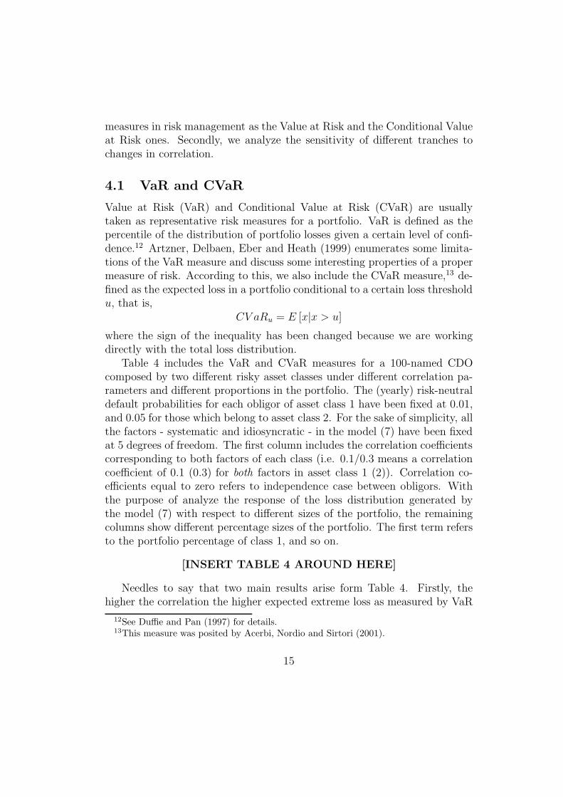
Table 2 displays the main results obtained. First row corresponds to thethree simulated base cases: the standard Gaussian model9 with one factor,two asset classes; the two assets-two Gaussian factor; finally, the two assets-two t-Student factors.10 t-Student distributions have been fixed at 5 degreesof freedom for idiosyncratic and systematic factors. Second row displays thecorrelation parameters of each asset class with both factors. For example,0.1/0.3 in the two Gaussian case refers to a correlation of 0.1 (0.3) for ele-ments of class 1 (2) with the two systematic factors. In line with Gregory andLaurent (2004), our idea is to check the behaviour of the CDO to a portfolioexposed to two different degrees of correlation.
[INSERT TABLE 2 AROUND HERE]
All the simulations have been carried on for different tranches values.Looking at the riskier tranche (equity tranche), we observe that, for thesame degree of correlation, its spread is systematically bigger for the two t-Student case than for the 2 Gaussian factors. One conclusion that arises fromTable 2 is that the two assets-one Gaussian factor spreads for equity trancheare close to those values obtained for two assets-two t-Student factors.
As expected, the same does not apply for mezzanine tranches: the addi-tion of more factors provides more weight to extreme default events, whichresults in an increase in spread of mezzanine tranches. The same conclusionsapply to senior tranche.
3.2 Approximation for n infinite
The asymptotic relationship between a t-distributed random variable anda normal random variable by means of the Cornish-Fisher expansion couldbe interesting for cases of big degrees of freedom. Shaw (2006) providesthe Cornish-Fisher expansion for a t-distributed random variable, with zeromean and unit variance, in terms of a standard normal random variabledistribution. This reduces considerably the computational time as, in this
9The standard Gaussian model has been computed using a Gauss-Hermite quadraturewith 8 nodes.
10The t-Student simulations have been computed using a Simpson’s quadrature with 25points.
13

case, it is possible to use a double Gauss-Hermite quadrature, instead of aSimpson quadrature. Basically, Shaw (2006) provides the relationship
s = z +1
4nz
(z2 − 3
)+
1
96n2z(5z4 − 8z2 − 69
)+ ... (9)
where s is the t-distributed random variable with n degrees of freedom, andz is a standard normal random variable. To check the accuracy of the ap-proximation (9), Table 3 displays the spreads (in basis points) for differenttranches in a two asset classes, 50-named CDO with quarterly payments un-der different correlation parameters for various degrees of freedom. As in theprevious section, correlation parameters correspond to factors of each assetclasses. As in previous examples, risk neutral default probabilities have beenalso fixed at 0.1 and 0.3 for each asset class. The recovery rate is fixed at40%.
[INSERT TABLE 3 AROUND HERE]
Basically, two general models have been computed: two Gaussian factorsand a two t-Student factor. The last column refers to the two t-Studentfactor approximation using the Cornish-Fisher expansion. Correlation co-efficients and degrees of freedom for each one are displayed in the table.11
The Gaussian case is presented to get intuition of how far we are from theasymptotic result. As expected, the larger the degree of freedom, the higherthe accuracy of the results. The differences between the equity tranche rangefrom 20% for 10 degrees of freedom to 12% for a 15 degrees of freedom case.In a similar way, considering the mezzanine cases, differences go from 21%to 11%. There are no substantial changes in the case of senior tranche. Itis worth to remember that computations under the exact t-Student distribu-tion have been done using a numerical quadrature and, so, they are exposedto numerical errors.
4 Sensitivity analysis
Now, we are interested in the prices of the CDO under two different scenarios:changes in portfolio size and correlation. Firstly, we present some standard
11The two Gaussian factor model is equivalent to a two t-Student factor model withinfinite degrees of freedom.
14
measures in risk management as the Value at Risk and the Conditional Valueat Risk ones. Secondly, we analyze the sensitivity of different tranches tochanges in correlation.
4.1 VaR and CVaR
Value at Risk (VaR) and Conditional Value at Risk (CVaR) are usuallytaken as representative risk measures for a portfolio. VaR is defined as thepercentile of the distribution of portfolio losses given a certain level of confi-dence.12 Artzner, Delbaen, Eber and Heath (1999) enumerates some limita-tions of the VaR measure and discuss some interesting properties of a propermeasure of risk. According to this, we also include the CVaR measure,13 de-fined as the expected loss in a portfolio conditional to a certain loss thresholdu, that is,
CV aRu = E [x|x > u]
where the sign of the inequality has been changed because we are workingdirectly with the total loss distribution.
Table 4 includes the VaR and CVaR measures for a 100-named CDOcomposed by two different risky asset classes under different correlation pa-rameters and different proportions in the portfolio. The (yearly) risk-neutraldefault probabilities for each obligor of asset class 1 have been fixed at 0.01,and 0.05 for those which belong to asset class 2. For the sake of simplicity, allthe factors - systematic and idiosyncratic - in the model (7) have been fixedat 5 degrees of freedom. The first column includes the correlation coefficientscorresponding to both factors of each class (i.e. 0.1/0.3 means a correlationcoefficient of 0.1 (0.3) for both factors in asset class 1 (2)). Correlation co-efficients equal to zero refers to independence case between obligors. Withthe purpose of analyze the response of the loss distribution generated bythe model (7) with respect to different sizes of the portfolio, the remainingcolumns show different percentage sizes of the portfolio. The first term refersto the portfolio percentage of class 1, and so on.
[INSERT TABLE 4 AROUND HERE]
Needles to say that two main results arise form Table 4. Firstly, thehigher the correlation the higher expected extreme loss as measured by VaR
12See Duffie and Pan (1997) for details.13This measure was posited by Acerbi, Nordio and Sirtori (2001).
15

and CVaR, as expected. Secondly, an increase in the percentage of the riskyasset (asset class 2) produces an increase in the losses of the portfolio.
4.2 Sensitivity to correlation
To analyze the sensitivity to correlation of the model (7) we have createda CDO based on a portfolio of 50 names. Individual default probabilitieshave been fixed at 1% for asset class 1 and 5% for asset class 2, respectively.To reduce the computational cost of the implementation, we have set thedistribution of the two systematic factors as t-Student ones with 15 degreesof freedom. We have used the results of Shaw (2006) developed in Section2.5, without loss of generality. All simulations have been performed using adouble Hermite quadrature with 64 nodes. Idiosyncratic factors have beenfixed at 5 for each asset class. To search differences in the portfolio com-position, we have applied our study to two different sized portfolio: equallyweighted portfolio (50% asset class 1, 50% asset class 2) and risky portfolio(25% asset class 1, 75% asset class 2).
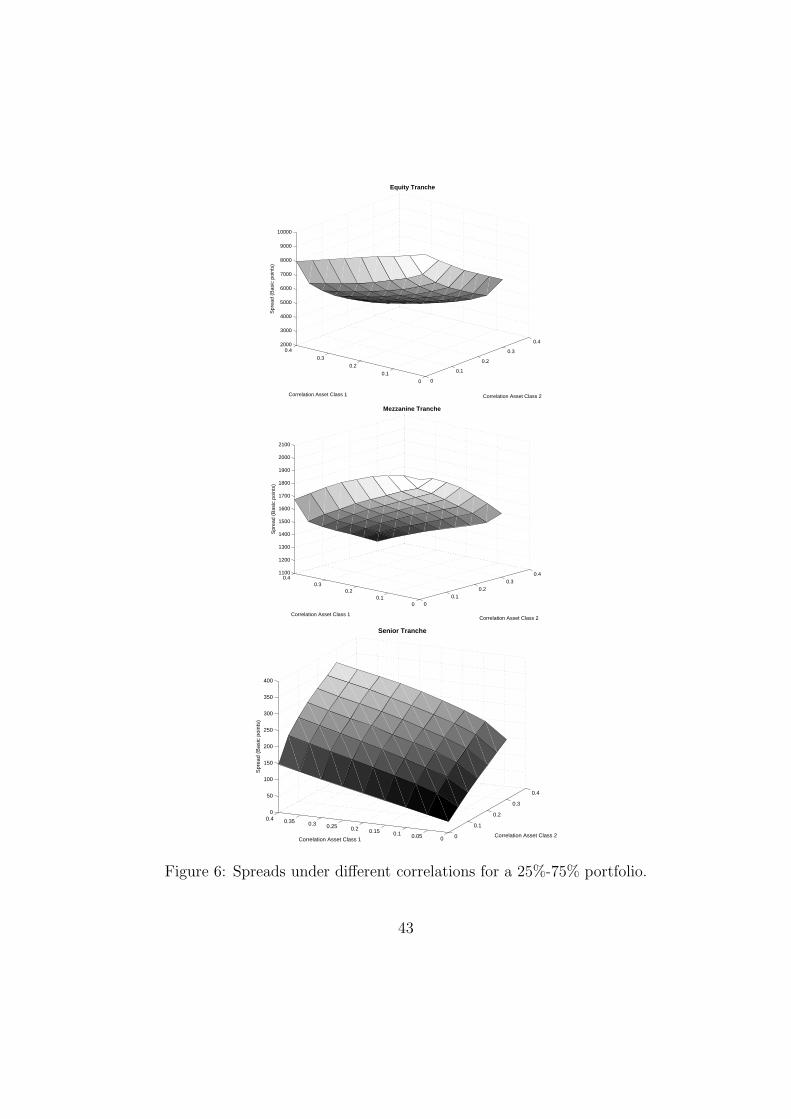
Figures 5 and 6 display the spreads obtained under different sets of corre-lations for the equally weighted and risky portfolios. In general, the convexitypattern of the equity-senior curves remains constant in both cases, which isconsistent with the preference (aversion) for risk on equity (senior) trancheinvestors, as expected.
Regarding changes in correlation, Figure 5 reveals that correlation withrisky asset classes are, by large, responsible of changes in the value of equityspreads. When it comes to the risky portfolio (Figure 6), it is interesting toobserve how changes produced by the correlation in asset class 1 or 2 (seeEquity and Mezzanine tranches) produce almost the same effects.
[INSERT FIGURE 5 AROUND HERE]
As also expected, an increase in global correlation raises the spreads ofsenior tranche. A higher correlation increases the probability of big losses,which is reflected in the senior spreads. This feature could be also mentioned(in a different scale) to the case of the risky portfolio in Figure 6.
[INSERT FIGURE 6 AROUND HERE]
16

5 Econometric Framework
This section focuses on the parameters estimation of the model (7). Aspointed out in Embretchs, Frey and McNeil (2005), the statistical estimationof parameters in many industrial models are simply assigned by means of
economic arguments or proxies variables. We will develop an exercise offormal estimation using some well known econometric tools as logit-probitregressions.14 Due to the features of our data, some cautions must be takento understand our results. This is due to the shortage of relevant data (forinstance, rates of default of high-rated companies) or the sample size, aswas also noticed by Embretchs, Frey and McNeil (2005). These authors alsoprovide a more general discussion on the statistical estimation of portfoliocredit risk models.
5.1 Estimation Techniques
As suggested by Schonbucher (2003) or Embretchs, Frey and McNeil (2005),the estimation of parameters in the expression (7) will be carried on using themodels for discrete choice of proportions data. Basically, the idea consistsin explaining the sample rates of default pi (where i refers to the asset classor group) as an approximation to the population rates of default Pi plus anerror term, εi. The idea behind is to link the population probability withsome function F (·) over a set of explanatory factors xi and their coefficientsβ, as follows:
pi = Pi + εi = F (x′
iβ) + εi (10)
To be interpreted as a probability, the function F (·) must be bounded andmonotonically increasing in the interval [0, 1]. Some widely used functionsfor F are the standard Normal distribution, which corresponds to the probitmodel, or the uniform distribution, which results in the linear probabilitymodel.
As suggested by Greene (2003), we could use regression methods as wellas maximum likelihood procedures to estimate the set of coefficients β ofthe expression (10). For example, in the case of the probit regression, therelationship between the sample rates of default pi and their population coun-
14Standard references on this type of regressions using grouped data can be found inNovales (1993) or Greene (2003).
17

terparts arepi = Pi + εi → Φ−1 (pi) = Φ−1 (Pi + εi)
which could be aproximated by (Novales, 1993)
Φ−1 (pi) ≃ x′
iβ+εi
f (x′
iβ)
where Φ (·) denotes the distribution function of a standard Normal variable.As mentioned in Novales (1993), the last expression suggests that we canestimate the parameter vector β by regressing the sample probits Φ−1 (pi) onthe variables x. Considerations about the heteroskedasticity of the residualcan be found in the cited reference.
To check the model’s goodness of fit, Novales (1993) also provides a com-parison of different regressions (probit, logit or lineal) in terms of the meansquare error (MSE) . The statistic s is defined as
s =
T∑
1
ni
(pi − Pi
)2
Pi
(1 − Pi
) ∼ χ2T−k (11)
where ni represents the sample size of the data (subscript i refers to asset class
or group) and pi, Pi are the observed and estimated frequencies, respectively.The statistic s follows a chi-square distribution with T−k degrees of freedom,sample length T and k restrictions.
5.2 Variables and estimation
With the intention of illustrating the estimation of the model (7), we havechosen a set of six explanatory variables for the rates of default: the realGrowth Domestic Product (GDP), the Consumers Price Index (CPI), theannual return on the S&P500 index (SP ret), its annualized standard devi-ation (SP std), the 10-year Treasury Constant Maturity Rate (10 rate) andthe Industrial Production Index (IPI).15 As dependent variables we have theannual rates of default for two investment grades: non investment grade (SG)and investment grade (IG), both collected from Hamilton, Varma, Ou and
15All data are available from the Federal Reserve Bank of St. Louis webpage(www.stlouisfed.org) except the S&P 500 index level, which has been taken fromBloomberg.
18

Cantor (2005). Due to the availability of default rate data, the sample pe-riod has been taken from 1970 to 2004, which results in 35 observations. Asummary of the main statistics and the correlation coefficients is presentedin Tables 5 and 6, respectively.
[INSERT TABLES 5 AND 6 AROUND HERE]
To visualize the influence of the proposed explanatory variables in thedefault rates, Figure 7 represents the scatter plots of non-investment graderates of default versus different explanatory variables. This figure seems tocorroborate what we could guess departing from the correlation parametersincluded in Table 6: the standard deviation of the S&P 500 returns, the GDPand the CPI can be good candidates for explaining the default rate in thecase of the non-investment firms. Additionally, at a certain degree, the S&P500 return can be added to this list as a possible explanatory variable in thecase of the investment firms.16
[INSERT FIGURE 7 AROUND HERE]
One step ahead is to compute how much of the sample can be explainedby the set of variables under study. To answer this question, we regress thenon-investment and investment rates on these explanatory variables. Table7 shows the results. The first row corresponds to the different independentvariables under study. The first column contains the model under study -linear, probit, logit - and the different regressed variables (SG and IG defaultrates). Second to eighth columns display different betas obtained underdifferent models. Finally, the last column shows the s statistic defined in (11),which will be used as a naive benchmark: if the whole set of independentvariables explains some quantity of the sample, two variables would explain“less”: the pair of variables whose s value are closest to the benchmark couldbe good candidates as common factors in the model (7).
[INSERT TABLE 7 AROUND HERE]
16A similar figure, available upon request, with investment grade rates of default wasbuilt but is omitted for the sake of brevity. However, this figure reveals that, due to thehigh number of null observations in the IG sample, conclusions about the factors affectingIG rates should be taken carefully.
19

We start with regressions on SG rates. One main reason recommendsthis procedure: their data are more relevant to determine which factors maycause default. Up to a point, conclusions on the factors will be more ro-bust. Previous regressions suggest choosing the variables GDP, CPI, IPI andSP stdas common factors in the model (7). These variables minimize thestatistic (11) with respect to other pairs of alternatives. Finally, we selectGDP and CPI as common factors according to two main reasons:
1. Firstly, the Industrial Production Index could be seen as a proxy of theGDP and its information could result redundant. Moreover, regressionsof probit-logit models using these two variables support the choice ofGDP against the IPI.
2. Secondly, regressions on the parameter SP std give a beta close to theprecision imposed to our estimated parameters (10−4).
Table 8 presents in columns the OLS17 estimates for betas of independentterm, GDP variable and CPI variable, respectively, using the SG rates. Con-fidence intervals at the 95% level are displayed into brackets. The rows inthis table also display regression results for linear, probit and logit models.The last row contains the value of the statistic (11) obtained for each case.Attending to the goodness-of-fit criteria using s, the OLS probit model re-gression provides the best fit to the sample18. Overall, all the beta estimatescorresponding to OLS regressions are negative, except for the independentterm of the linear model, which leads to higher s statistic. Results concerningto OLS regressions can be interpreted as follows: a negative beta implies anincreasing on default probabilities. In line with this, as expected, a decreasein GDP rates may produce an increase on SG default rates. Surprisingly,an increase in the CPI rate could diminish the rates of default, which mightresult counter-intuitive.
Table 9 shows regression results for linear, probit and logit models usingIG rates as dependent variable. It is worth to notice that results are notconclusive as 63% of the sample under study are zeros. GLS estimationsdo not make sense in this context. In order to avoid numerical problemsin the estimation, we have added the quantity 0.00005 to the sample, as
17GLS estimates have not been computed due to the sample size.18Maximum Likelihood estimates (available upon request) for models probit and logit
are close to those parameters obtained for respective OLS models.
20

suggested by Greene (2003). The first row displays the independent termand explanatory variables. Each pair of the following rows contains firstlythe different values of betas obtained using two variables (GDP and CPI);secondly, their values using only the GDP variable. Maximum likelihoodestimates (available upon request) for the probit and logit models are closeto those parameters obtained for respective OLS models. We have estimatedGDP variable alone with the intention of analyzing the explanatory power ofthe GDP on IG rates. First to second rows show the model and procedureused. The last column displays the value for the statistic s. At a certaindegree, results on Table 8 could support the inverse relationship between theexplanatory variables and the IG rates of default, as previously noted for theSG case.
[INSERT TABLES 8 AND 9 AROUND HERE]
5.3 Interpretation of coefficients
As pointed out by Elizalde (2005), due to the difficulty of interpreting whatthe correlation term represents, estimating the correlation term in factormodels is not an evident task. Looking at equation (10), the estimate β de-scribes the effect from the explanatory factor x through a non-linear trans-formation of the firm’s asset value, which itself is unobserved, as it is alsonoticed by Elizalde (2005). As this fact complicates understanding the propercorrelation term, the author enumerates some measures used ad hoc by prac-titioners, as equity return correlations, to conclude about the insufficiency(and scarcity) of papers that deals with this problem.
Our interpretation of coefficients in the model (7) goes in the direction ofthe econometric explanation for the coefficients of the linear, logit and probitmodels, that is, the influence of the exogenous variables on the endogenousone. In other words, the (relative) impact of the explanatory variables onthe probability of default. Following Novales (1993), this interpretation ofestimates for the linear model must differ to that for the logit and probitmodels.19 This is the main reason why we split our results in two tables,Tables 10 and 11, that include - respectively - the estimation of the linearand logit-probit models.
19For example, the relationship between the explanatory and explained variables in theprobit model is non-linear while the linear probability model implies linearity betweendependent and independent variables.
21

[INSERT TABLES 10 AND 11 AROUND HERE]
Regarding the estimates of the linear probability model, Table 10 reflectsthe contribution of the two explanatory random variables to the probability ofdefault. The main conclusions are obtained from the default probabilities ofnon-investment grade assets (SG), but can also be extended to the investmentgrade (IG) ones. Looking at Table 10, it is interesting to observe the sign ofthe coefficients, which is negative: the more we decrease the GDP or the CPI,the more we increase the rates of default. Given the value of the coefficients,the variables have the same contribution to the default probability. Withreference to the fit of the model to the data, under the null hypothesis thatthe goodness-of-fit to the sample is good, we cannot reject that the linearprobability model could explain the results obtained.
Table 11 includes the ratio between estimates for SG and IG series forprobit and logit models, respectively. By and large, the conclusions arethe same for all the series under study. According to Novales (1993), theratio between the estimated betas measures the relative contribution of theexplanatory variables on the default probability. Results are consistent tothose obtained for the linear probability model: the negative sign of theexplanatory variables, which reflects an opposite effect between default ratiosand the macroeconomic variables. Moreover, the relative contribution ofthe explanatory variables remains equal, as was also derived from Table 10.Finally, we do not reject the goodness-of-fit of the model using confidencelevels of 95% and 99%.
6 Conclusions
The current success of the credit derivatives market for tranched productsis one of the biggest ones seen within the financial industry. The standardpricing model, widely used by the practitioners, is the Gaussian one-factormodel (Vasicek, 1991). However, some assumptions underlying this modelare probably too restrictive. These features concern, among others, to thoseof homogeneity of asset classes involved, or the exposure to one sources ofsystematic risk.
In a more realistic setting, Schonbucher (2003) or Lando (2004) pointedout that a credit portfolio is composed by different asset classes or buckets,attending to criteria as, for example, investment grade, non-investment grade
22

assets or industry. The exposure of a credit portfolio to a set of commonrisk factors could be significant between groups, but should be homogeneouswithin them. In line with this, the idea of two groups of assets treatedin different ways could become a more realistic assumption than that usedpreviously in the literature.
With the aim of contributing to the current literature, this article hasconsidered a family of models that takes into account the existence of dif-ferent asset classes or regions of correlation. In more detail, this paper hasgeneralized the two assets-two Gaussian factor model of Schonbucher (2004)by proposing a two by two model (two factors and two asset classes). Weassume two driving factors (business cycle and industry) with independentt-Student distributions, respectively, and allow the model to distinguish be-tween portfolio assets classes. It may be worth noting that one of the mainimplications from considering the t-Student distribution is that we assign ahigher probability to high default events.
Our work contributes to the existing literature in the analysis of theseasset class models. To the best of our knowledge, no similar study has beenreported yet in this direction. Regarding the distributional assumptions, wehave extended the standard Gaussian model by considering the t-Studentdistribution. In this way, we have dealt with a more general model with theadditional advantage that includes the Gaussian model as a particular case.We have also provided the econometric framework for assessing the param-eters of the posited model. Finally, an empirical application with Moody’sdata has been presented as an illustration of the methodology proposed.
After proposing several explanatory variables, it seems that the standarddeviation of the S&P 500 returns, the GDP and the CPI can be good candi-dates for explaining the default rates in non-investment firms. Additionally,at a certain degree, the S&P 500 return can be added to the previous ones toexplain the default rates for investment firms. Additionally, a more detailedstudy leads to select GDP and CPI as common factors.
Focusing on OLS estimates, it is seen that - as expected - a decrease inGDP rates may produce an increase on SG default rates. Surprisingly, it isalso obtained that an increase in the CPI rate can diminish the default ratesRegarding the estimates of the linear probability model, we see that the morewe decrease the GDP or the CPI, the more we increase the rates of default.
Finally, the ratio between estimates for SG and IG series for probit andlogit models has been analyzed. The conclusions are the same for all theseries under study and the results are consistent to those for the linear prob-
23

ability model: there is a negative relationship between default ratios and themacroeconomic variables. Deeper explanation for these empirical findingswill be the subject of further research.
24

References
[1] Acerbi, C., Nordio, C. and Sirtori, C. (2001): Expected Shortfall as aTool for Financial Risk Management, Working Paper, Italian Associa-tion for Financial Risk Management.
[2] Andersen, L., Sidenius, J. and Basu, S. (2003): All your hedges in onebasket, Risk, November: 67–72.
[3] Artzner, P., Delbaen, F., Eber, J.M. and Heath, D. (1999) CoherentMeasures of Risk, Mathematical Finance, 9: 203–208.
[4] BBA Credit Derivatives Report (2006).
[5] Bielecki,A. and F. Rutkowski (2002): Credit Risk, Springer.
[6] Black, F. and Cox, J.C. (1976): Valuing Corporate Securities: SomeEffects of Bond Indenture Provisions, Journal of Finance, 31: 351–367.
[7] Duffie, D. and Garlenau, N. (2001): Risk and Valuation of CollateralizedDebt Obligations, Financial Analysts Journal, January/February: 41–59.
[8] Duffie, D. and Pan, J. (1997): An overview of VaR, Journal of Deriva-
tives, 4: 98–112.
[9] Elizalde, A. (2005): Credit Risk Models IV: Understanding and pricingCDOs, Working Paper, CEMFI, (available at www.abelelizalde.com).
[10] Gibson, M. S. (2004): Understanding the Risk of Synthetic CDOs,Working Paper 2004-36, Federal Reserve Board.
[11] Glasserman, P. and Suchitabandid, S. (2006): Correlation Expansionsfor CDO Pricing, to appear in Journal of Banking and Finance.
[12] Green, W. H. (2003): Econometric Analysis, 5th edition. Pearson Edu-cation, New Jersey.
[13] Gregory, J. and Laurent, J.P. (2004): In the Core of Correlation, Risk,October: 87–91.
[14] Gregory, J. and Laurent, J.P. (2005): Basket Default Swaps, CDO’s andFactor Copulas, Journal of Risk, 7, 4, 103–122.
25

[15] Gupton, G., Finger, C. and Bhatia, M. (1997): CreditMetrics. Technicaldocument, JPMorgan, April. www.creditmetrics.com
[16] Hamilton, D. T., Varma, P., Ou, S. and Cantor, R. (2005): Default andRecovery Rates of Corporate Bond Issuers, 1920-2004, Moody’s InvestorService, January.
[17] Hull, J. and White, A. (2004): Valuation of a CDO and an n-th toDefault CDS Without Monte Carlo Simulation, Journal of Derivatives,Winter: 8–23.
[18] Lucas, A., Klaassen, P., Spreij, P. and Staetmans, S. (2001): An ana-lytic approach to credit risk of large corporate bond and loan portfolios,Journal of Banking and Finance, 25 (9): 1635-1664.
[19] Longstaff, F. A. and Rajan, A. (2006): An empirical analysis of the pric-ing of collateralized debt obligations, Working Paper, UCLA AnderssonSchool.
[20] Mashal, R. and Naldi, M. (2002): Calculating portfolio loss, Risk, Au-gust: 82–86.
[21] Mardia, K. V., Kent, J. T. and Bibby, J. (1979): Multivariate Analysis,Ed. Academic Press, London.
[22] Merton, R. C. (1974): On the Pricing of Corporate Debt: The RiskStructure of Interest Rates, Journal of Finance, 29: 449-470.
[23] Novales, A. (1993): Econometrıa, 2a ed. McGraw-Hill, Madrid.
[24] Tavakoli, J. M. (2003): Collateralized Debt Obligations and StructuredFinance. New Developments in Cash and Synthetic Securitization, JohnWiley and Sons, Inc., Hoboken, New Jersey.
[25] Vasicek, O. (1991): Limiting Loan Loss Probability Distribution, KMVCorporation.
26

Table 1: Spreads of different tranches for a 100-names CDO under different correlation parameters
Model Standard Gaussian 2 Gaussian factors t-StudentCorrelation 0.1 0.3 0.1/0.1 0.1/0.3 0.1 0.3
Attachment points (%) Tranche Spread (basis points)
0–3 2117 1320 2186 1656 2485 21353–10 86 110 508 653 131 233
10–100 0.02 1 7 29 1 9
27
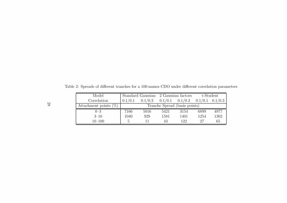
Table 2: Spreads of different tranches for a 100-names CDO under different correlation parameters
Model Standard Gaussian 2 Gaussian factors t-StudentCorrelation 0.1/0.1 0.1/0.3 0.1/0.1 0.1/0.3 0.1/0.1 0.1/0.3
Attachment points (%) Tranche Spread (basis points)
0–3 7166 5016 5421 3154 6899 49773–10 1040 929 1581 1401 1254 1302
10–100 5 11 43 122 27 65
28

Table 3: Spreads of different tranches for a 50-names CDO under different correlation parameters
Model 2 Gaussian factors t-Student CF t-StudentCorrelation 0.1/0.3 0.1/0.3 0.1/0.3 0.1/0.3 0.1/0.3
Degrees of freedom (n1/n2) ∞/∞ 10/10 15/15 10/10 15/15
Attachment points (%) Tranche Spread (basis points)
0–3 3015 3924 3711 3270 32963–10 1380 1236 1198 1025 1083
10–100 289 160 160 166 160
29

Table 4: VaR and CVaR measures for a 100-named CDO composed by two different risky asset classes underdifferent correlation parameters and different proportions in the portfolio. Degrees of freedom are fixed at5 for all factors. The first (second) coefficient refers to the percentage proportion of Asset Class 1 (2) inthe portfolio. Yearly risk-neutral probabilities have been fixed to 0.01 for each obligor of Asset Class 1, and0.05 for those of Asset Class 2.
VaR 99% CVaR 99%Correlation 25/75 50/50 75/25 25/75 50/50 75/25
0.0/0.0 10 9 7 18 9 90.1/0.1 25 19 13 35 27 190.1/0.3 57 40 23 67 48 300.3/0.3 61 47 33 72 61 50
30

Table 5: Descriptive Statistics
Descriptive Statistics mean median std skewness kurtosis max min
IG 0.0006 0 0.0011 2.2481 8.2051 0.0049 0SG 0.0389 0.0345 0.0288 1.0213 3.0976 0.1058 0.0042
SP ret 0.0297 0.0439 0.0675 -0.6110 2.5129 0.1310 -0.1208SP std 89.4702 39.3947 106.3397 1.4176 3.7198 390.1884 7.5537GDP 0.0130 0.0148 0.0087 -0.6077 2.8766 0.0301 -0.0085CPI 0.0205 0.0159 0.0128 1.2338 3.7824 0.0564 0.0052
10 rate 7.7577 7.4176 2.4231 0.8413 3.2283 13.9214 4.0139IPI 0.0111 0.0124 0.0185 -0.4614 3.2866 13.9214 -0.0409
31
Table 6: Correlation matrix
IG SG SP ret SP std GDP CPI 10 rate IPI
IG 1.0000SG 0.4106 1.0000
SP ret -0.2388 -0.2153 1.0000SP std 0.1760 0.3472 -0.0424 1.0000GDP -0.1431 -0.3541 0.4988 0.0029 1.0000CPI -0.1847 -0.3209 -0.2806 -0.4959 -0.4937 1.0000
10 rate -0.1043 -0.2344 0.0611 -0.6113 -0.1070 0.6060 1.0000IPI -0.1499 -0.2930 0.2687 -0.0385 0.6671 -0.3252 -0.1344 1.0000
32
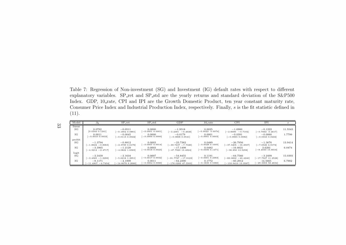
Table 7: Regression of Non-investment (SG) and Investment (IG) default rates with respect to differentexplanatory variables. SP ret and SP std are the yearly returns and standard deviation of the S&P500Index. GDP, 10 rate, CPI and IPI are the Growth Domestic Product, ten year constant maturity rate,Consumer Price Index and Industrial Production Index, respectively. Finally, s is the fit statistic defined in(11).
Model β0 SP ret SP std GDP 10 rate CPI IPI s
linear
SG 0.0792[0.0344 0.1241]
−0.0511[−0.1904 0.0881]
0.0000[−0.0001 0.0001]
−1.9518[−3.4391 −0.4646]
0.0025[−0.0022 0.0074]
−1.6900[−2.6699 −0.7102]
−0.1222[−0.7063 0.4617]
11.5543
IG 0.0011[−0.0010 0.0033]
−0.0045[−0.0113 0.0022]
0.0000[−0.0000 0.0000]
−0.0179[−0.0898 0.0541]
0.0001[−0.0001 0.0003]
−0.0391[−0.0865 0.0082]
−0.0060[−0.0343 0.0222]
1.7799
probit
SG −1.3794[−1.8624 −0.8963]
−0.8812[−2.3799 0.6176]
0.0003[−0.0007 0.0014]
−23.7382[−39.7437 −7.7326]
0.0489[−0.0028 0.1005]
−26.7956[−37.3405 −16.2507]
−1.3676[−7.6526 4.9174]
13.9414
IG −3.3965[−4.3212 −2.4717]
−1.2129[−4.0822 1.6565]
0.0003[−0.0018 0.0023]
−17.1498[−47.7920 13.4924]
0.0482[−0.0506 0.1471]
−16.6621[−36.850 13.5258]
3.6291[−8.4033 15.6616]
6.0474
logit
SG −2.3439[−3.4585 −1.2293]
−2.1634[−5.6218 1.2951]
0.0007[−0.0017 0.0032]
−54.8455[−91.7787 −17.9123]
0.1191[−0.0001 0.2383]
−64.7566[−89.0892 −40.4240]
−3.2499[−17.7527 11.2528]
15.0393
IG −8.1171[−11.4907 −4.7434]
−4.1999[−14.6678 6.2680]
0.0011[−0.0064 0.0086]
−64.2390[−176.0283 47.5503]
0.1772[−0.1835 0.5380]
−60.2912[−133.9410 13.3587]
14.5665[−29.3303 58.4634]
6.7882
33

Table 8: Results for regressions of Non-investment (SG) default rates on real Growth Domestic Product(GDP) and Consumer Price Index (CPI) as explanatory variables.
SG Model β0 GDP CPI s
linear OLS 0.0979[0.0733 0.1226]
−2.2380[−3.2486 −1.2274]
−1.4690[−2.1548 −0.7832]
21.8030
probit OLS −1.0785[−1.3568 −0.8002]
−26.7705[−38.1822 −15.3587]
−21.6288[−29.3730 −13.8846]
14.7653
logit OLS −1.6293[−2.2769 −0.9816]
−61.8990[−88.4563 −35.3416]
−51.7790[−69.8014 −33.7567]
15.4018
34

Table 9: Results for regressions of Investment (IG) default rates on real Growth Domestic Product (GDP)and Consumer Price Index (CPI) as explanatory variables.
IG Model β0 GDP CPI s
linear OLS 0.0017[0.0005 0.0029]
−0.0391[−0.0884 0.0102]
−0.0290[−0.0624 0.0045]
5.0921
OLS 0.0009[0.0002 0.0015]
−0.0181[−0.0623 0.0261]
– 2.2557
probit OLS −3.1421[−3.6496 −2.6347]
−14.1617[−34.9687 6.6453]
−11.2345[−25.3546 2.8856]
6.4347
OLS −3.4781[−3.7663 −3.1899]
−5.9888[−24.5193 12.5417]
– 8.6336
logit OLS −7.1801[−9.0318 −5.3284]
−50.7973[−126.7275 25.1328]
−40.7355[−92.2634 10.7923]
7.1658
OLS −8.3983[−9.4493 −7.3472]
−21.1631[−88.7533 46.4271]
– 9.6372
35

Table 10: Estimated coefficients for the linear probability model. s refers to the fit statistic.
Linear model β0 GDP CPI s χ295% (32) χ2
99% (32)
SG 0.0979 -2.2380 -1.4690 21.8030 No reject No rejectIG 0.0017 -0.0391 -0.0290 5.0921 No reject No reject
36

Table 11: Estimated coefficients for probit and logit models. s refers to the fit statistic.
β0GDPCPI
s χ295% (32) χ2
99% (32)
Probit modelSG -1.0785 1.2377 14.7653 No reject No rejectIG -3.1421 1.2606 6.4347 No reject No reject
Logit modelSG -1.6293 1.1954 15.4018 No reject No rejectIG -7.1801 1.2470 7.1658 No reject No reject
37

0 5 10 15 20 25 30 35 40 45 500
0.02
0.04
0.06
0.08
0.1
0.12Portfolio Losses
Number of firms
Pro
babi
lity
Standard Gaussian modelDouble−t model2−Gaussian factor model
Figure 1: Total loss distribution of a 100-firms portfolio for different models.Individual default probabilities are fixed at 1%. Correlation for the Stan-dard Gaussian and t-Student distribution (with 6 degrees of freedom) is 0.3.Correlations for the Double Gaussian model are 0.1, 0.3.
38

0 5 10 15 20 25 300
2
4
6
8
10
12Default rates by year
Years
Rat
es o
f def
ault
(%)
IGSG
Figure 2: Default (yearly) rates for Investment and Non-investment grades.Rates for investment data have been multiplied by ten with the purpose ofcomparing the data. Source: Moody’s.
39

1975 1980 1985 1990 1995 2000−0.5
0
0.5
1
Years
Cor
rela
tion
coef
ficie
nt
Figure 3: Correlation coefficients using a moving window of 5 years.
40
0 5 10 15 20 25 30 35 40 45 500
0.02
0.04
0.06
0.08
0.1
0.12Portfolio Losses
Number of firms
Pro
babi
lity
Standard Gaussian modelDouble−t model2−by−2 Double−t model
Figure 4: Total loss distribution of a 100-firms portfolio for standard Gaus-sian, Double-t and 2-by-2 Double-t model. Degrees of freedom in the double-tmodels have been fixed at six for every variable. Individual default proba-bilities are fixed at 10% for asset class A and 15% for asset class B. Allfirms in Gaussian and Double-t cases belong to asset class A. The portfolioin the 2-by-2 Double-t model is equally composed of asset classes A and B.Finally, correlation for the standard Gaussian model and Double-t is 0.2, andcorrelations for the Double-t model are 0.1, 0.2, respectively.
41

00.1
0.20.3
0.4
0
0.1
0.2
0.3
0.42000
3000
4000
5000
6000
7000
8000
Correlation Asset Class 2
Equity Tranche
Spr
ead
(Bas
ic p
oint
s)
Correlation Asset Class 1
0
0.1
0.2
0.3
0.4
00.050.10.150.20.250.30.350.4
950
1000
1050
1100
1150
1200
1250
1300
Correlation Asset Class 2
Mezzanine Tranche
Correlation Asset Class 1
Spr
ead
(Bas
ic p
oint
s)
0
0.1
0.2
0.3
0.4
00.1
0.20.3
0.40
50
100
150
200
250
Correlation Asset Class 2
Senior Tranche
Correlation Asset Class 1
Spr
ead
(Bas
ic p
oint
s)
Figure 5: Spreads under different correlations for a equally weighted (50%-50%) portfolio.
42
0
0.1
0.2
0.3
0.4
0
0.1
0.2
0.3
0.42000
3000
4000
5000
6000
7000
8000
9000
10000
Correlation Asset Class 2
Equity Tranche
Correlation Asset Class 1
Spr
ead
(Bas
ic p
oint
s)
00.1
0.20.3
0.4
00.1
0.20.3
0.41100
1200
1300
1400
1500
1600
1700
1800
1900
2000
2100
Correlation Asset Class 2
Mezzanine Tranche
Correlation Asset Class 1
Spr
ead
(Bas
ic p
oint
s)
0
0.1
0.2
0.3
0.4
00.050.10.150.20.250.30.350.40
50
100
150
200
250
300
350
400
Correlation Asset Class 2
Senior Tranche
Correlation Asset Class 1
Spr
ead
(Bas
ic p
oint
s)
Figure 6: Spreads under different correlations for a 25%-75% portfolio.
43

0 0.05 0.1 0.15 0.2−0.2
−0.1
0
0.1
0.2
SG Rates
SP
ret
0 0.05 0.1 0.15 0.20
100
200
300
400
SG RatesS
Pstd
0 0.05 0.1 0.15 0.2−0.02
0
0.02
0.04
SG Rates
GD
P
0 0.05 0.1 0.15 0.20
5
10
15
SG Rates
10rat
e
0 0.05 0.1 0.15 0.20
0.02
0.04
0.06
SG Rates
CP
I
0 0.05 0.1 0.15 0.2−0.05
0
0.05
SG Rates
IPI
Figure 7: Non-investment grade rates of default (SG) versus different ex-planatory variables
44