DEGREE PROJECT, IN , SECOND LEVELMATHEMATICAL STATISTICS

STOCKHOLM, SWEDEN 2015

Pricing Interest Rate Derivatives in theMulti-Curve Framework with aStochastic Basis

ZAKARIA EL MENOUNI

KTH ROYAL INSTITUTE OF TECHNOLOGY

SCI SCHOOL OF ENGINEERING SCIENCES

Pricing Interest Rate Derivatives in the Multi-Curve Framework with a

Stochastic Basis

Z A K A R I A E L M E N O U N I

Degree Project in Mathematical Statistics (30 ECTS credits) Degree Programme in Engineering Physics (300 credits)

Royal Institute of Technology year 2015 Supervisor at Dexia, France, was Gianmarco Capitanio

Supervisor at KTH was Filip Lindskog Examiner was Filip Lindskog

TRITA-MAT-E 2015:09 ISRN-KTH/MAT/E--15/09--SE Royal Institute of Technology School of Engineering Sciences KTH SCI SE-100 44 Stockholm, Sweden URL: www.kth.se/sci

Aknowledgments

My master thesis within Dexia Credit Local has been a fulfilling and en-riching work experience, mostly thanks to the genuine help and supervision Iwas lucky to have.

For that I would like to thank the whole team of Market Model Validationbeginning with my supervisor Gianmarco Capitanio who has guided me intocarrying out a very interesting master thesis with a high degree of autonomy.

My grateful thanks also go to Pascal Oswald for welcoming me warmly inthe team and giving me the responsibility to conduct an interesting validationwork allowing me to discover the validation field and apprehend the type ofproblematics a quantitative analyst within market models validation deals withevery day.

I also want to thank Filip Lindskog for his supervision and interest in mywork and for giving me constructive feedback.

Finally, I want to express my gratitude to everyone who has helped makingmy stay in Sweden one of my greatest experiences, so much that I would considercoming back as soon as possible.

Zakaria El Menouni

Paris, March 2015.

2

Abstract

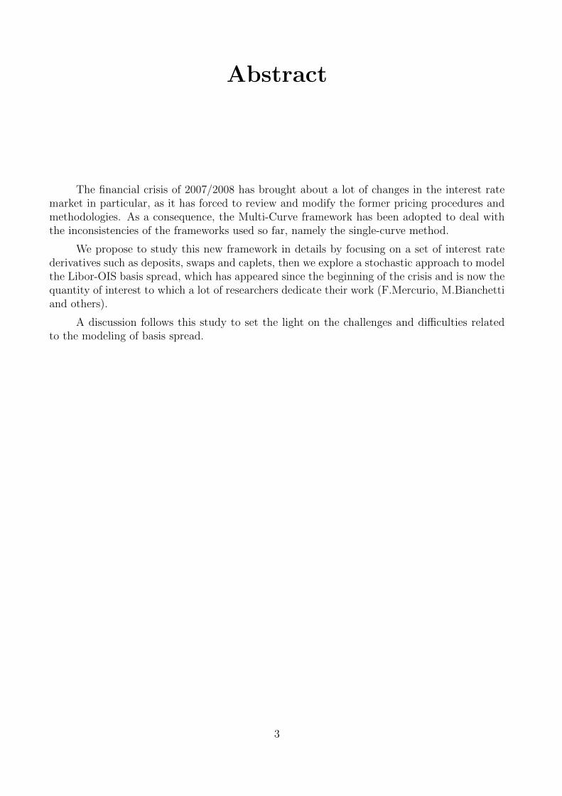
The financial crisis of 2007/2008 has brought about a lot of changes in the interest ratemarket in particular, as it has forced to review and modify the former pricing procedures andmethodologies. As a consequence, the Multi-Curve framework has been adopted to deal withthe inconsistencies of the frameworks used so far, namely the single-curve method.

We propose to study this new framework in details by focusing on a set of interest ratederivatives such as deposits, swaps and caplets, then we explore a stochastic approach to modelthe Libor-OIS basis spread, which has appeared since the beginning of the crisis and is now thequantity of interest to which a lot of researchers dedicate their work (F.Mercurio, M.Bianchettiand others).

A discussion follows this study to set the light on the challenges and difficulties relatedto the modeling of basis spread.

3

Sammanfattning

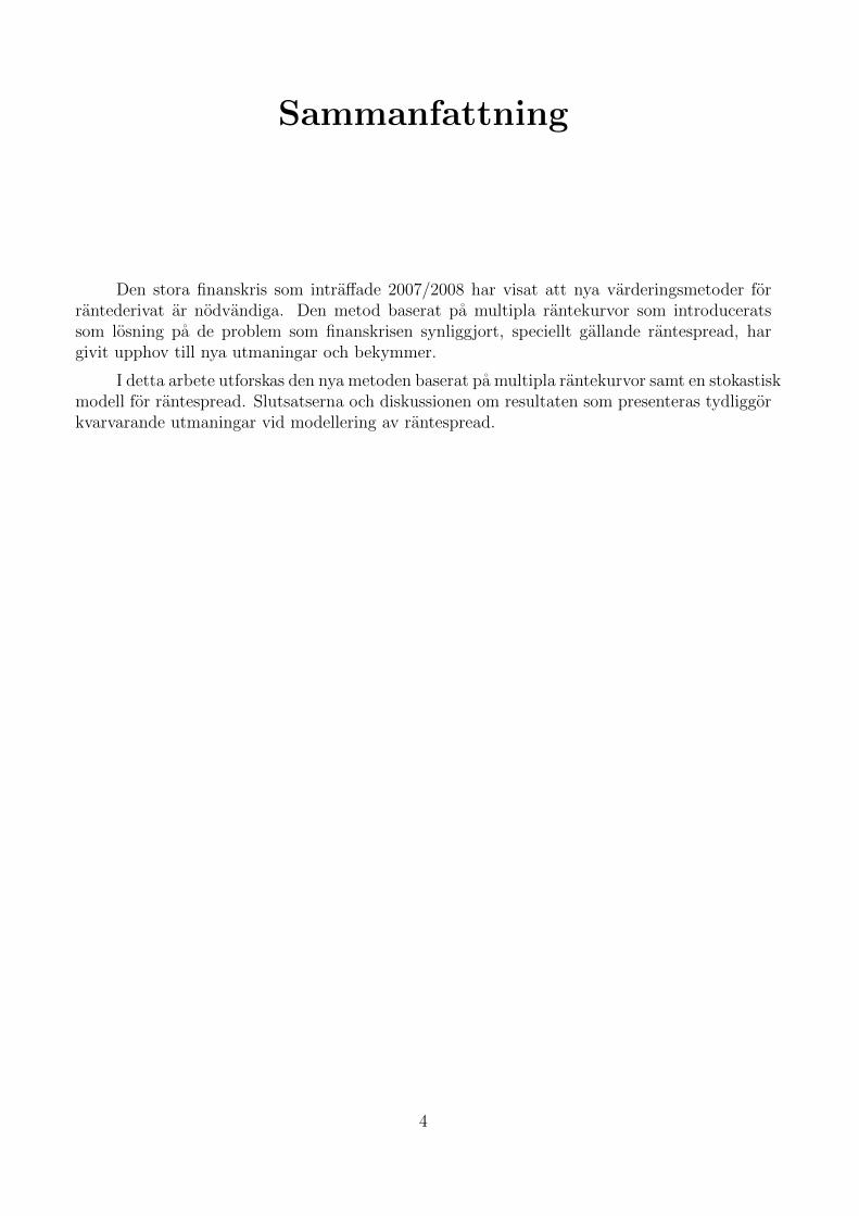
Den stora finanskris som intraffade 2007/2008 har visat att nya varderingsmetoder forrantederivat ar nodvandiga. Den metod baserat pa multipla rantekurvor som introduceratssom losning pa de problem som finanskrisen synliggjort, speciellt gallande rantespread, hargivit upphov till nya utmaningar och bekymmer.

I detta arbete utforskas den nya metoden baserat pa multipla rantekurvor samt en stokastiskmodell for rantespread. Slutsatserna och diskussionen om resultaten som presenteras tydliggorkvarvarande utmaningar vid modellering av rantespread.

4

Contents

Overview 7

Definitions and Key Words 8

Goals and Recurrent Notations 10

1 The Multi-Curve Framework 11

1.1 Interest Rate Spread Increase . . . . . . . . . . . . . . . . . . . . . . . . . . . . 11

1.2 Market Segmentation . . . . . . . . . . . . . . . . . . . . . . . . . . . . . . . . . 13

1.3 Pricing of Interest Rate Derivatives in the Multi-Curve Framework . . . . . . . . 14

1.3.1 The FRA rate . . . . . . . . . . . . . . . . . . . . . . . . . . . . . . . . . 14

1.3.2 The No-Arbitrage Pricing Formula . . . . . . . . . . . . . . . . . . . . . 15

1.3.3 Pricing Formulae for Plain Vanilla Instruments . . . . . . . . . . . . . . 16

1.4 Curve Construction in the Multi-Curve Framework . . . . . . . . . . . . . . . . 18

1.4.1 Example: The OIS Discount Curve . . . . . . . . . . . . . . . . . . . . . 19

1.4.2 Example: Pricing of an IRS in the Multi-Curve Setting . . . . . . . . . . 23

2 Modeling the Stochastic Basis Spread 25

2.1 The positivity of the Libor - OIS spread . . . . . . . . . . . . . . . . . . . . . . 25

2.2 Choice of The Model for the Stochastic Basis Spread . . . . . . . . . . . . . . . 26

2.3 Context and Notations . . . . . . . . . . . . . . . . . . . . . . . . . . . . . . . . 26

2.4 Caplet Pricing . . . . . . . . . . . . . . . . . . . . . . . . . . . . . . . . . . . . . 27

3 Case Study 30

3.1 Dynamics for the Forwards OIS Rates and the Spread . . . . . . . . . . . . . . . 30

3.2 Caplet Pricing Formula . . . . . . . . . . . . . . . . . . . . . . . . . . . . . . . . 32

3.3 Monte Carlo Method . . . . . . . . . . . . . . . . . . . . . . . . . . . . . . . . . 36

3.4 Model Calibration to Market Caplet Data . . . . . . . . . . . . . . . . . . . . . 37

3.5 Numercial Results and Discussion . . . . . . . . . . . . . . . . . . . . . . . . . . 38

4 Annex 44

4.1 Demonstrations . . . . . . . . . . . . . . . . . . . . . . . . . . . . . . . . . . . . 44

4.2 Market Data . . . . . . . . . . . . . . . . . . . . . . . . . . . . . . . . . . . . . . 44

References 48

5

List of Figures

1 OIS - EURIBOR 3M spread in %, EURIBOR 3M in white, OIS 3M in orangeand spread in yellow (lower graph) - Bloomberg data. . . . . . . . . . . . . . . . 11

2 Up: Scenario of a bond exchange between A (seller) and B (buyer), where B alsobuys a CDS from A to protect itself from an eventual default. Down: Scenarioof a bond exchange between A (seller) and B (buyer), without CDS. Red arrowscorrespond to the event of default (probability p) and the blue ones to the eventof non default (probability 1− p). . . . . . . . . . . . . . . . . . . . . . . . . . . 13

3 IRS cash flow diagram. . . . . . . . . . . . . . . . . . . . . . . . . . . . . . . . . 17

4 OIS cash flow diagram. . . . . . . . . . . . . . . . . . . . . . . . . . . . . . . . . 20

5 Up: OIS discount curve as of 01/10/2014, linear interpolation on the zero rates,down: Quoted interest rates. . . . . . . . . . . . . . . . . . . . . . . . . . . . . . 22

6 Caplet maturing at Tmk−1 and paying off at Tmk . . . . . . . . . . . . . . . . . . . . 27

7 Market and model (formula / MC) caplet prices comparison as of 01/10/2014,notional = 1. . . . . . . . . . . . . . . . . . . . . . . . . . . . . . . . . . . . . . 40

8 Calibration errors as of 01/10/2014. . . . . . . . . . . . . . . . . . . . . . . . . . 41

9 Market and model caplet prices comparison as of 01/10/2014 when using a modelwith a deterministic basis spread: σ6M

k = 0.335, σ6Mk = 0.379 and σ6M

k = 0.485for 3Y, 4Y and 6Y maturities respectively, notional = 1. . . . . . . . . . . . . . 42

List of Tables

1 Characteristics of the swap to be priced. . . . . . . . . . . . . . . . . . . . . . . 23

2 Pricing of the swap as of 30/09/2014. . . . . . . . . . . . . . . . . . . . . . . . . 23

3 Results of the calibration as of 01/10/2014. . . . . . . . . . . . . . . . . . . . . . 39

4 Pricing of the 3Y maturity caplet as of 01/10/2014 (comparison between ana-lytical and Monte Carlo results): Model prices ' Market prices. . . . . . . . . . 39

5 Pricing of the 4Y maturity caplet as of 01/10/2014 (comparison between analyt-ical and Monte Carlo results): Model prices ' Market prices (less accurate thanfor 3Y). . . . . . . . . . . . . . . . . . . . . . . . . . . . . . . . . . . . . . . . . 39

6 Pricing of the 6Y maturity caplet as of 01/10/2014 (comparison between ana-lytical and Monte Carlo results): Model prices 6= Market prices. . . . . . . . . . 39

7 Market quotes for the instruments used in bootstrapping the EUR OIS dis-count curve as of 01/10/2014. . . . . . . . . . . . . . . . . . . . . . . . . . . . 45

8 Market quotes for the instruments used in bootstrapping the EURIBOR 6Mforward curve as of 01/10/2014. . . . . . . . . . . . . . . . . . . . . . . . . . . 46

9 Market cap implied volatilities in (%) as of 01/10/2014. . . . . . . . . . . . . . . 47

6

Overview

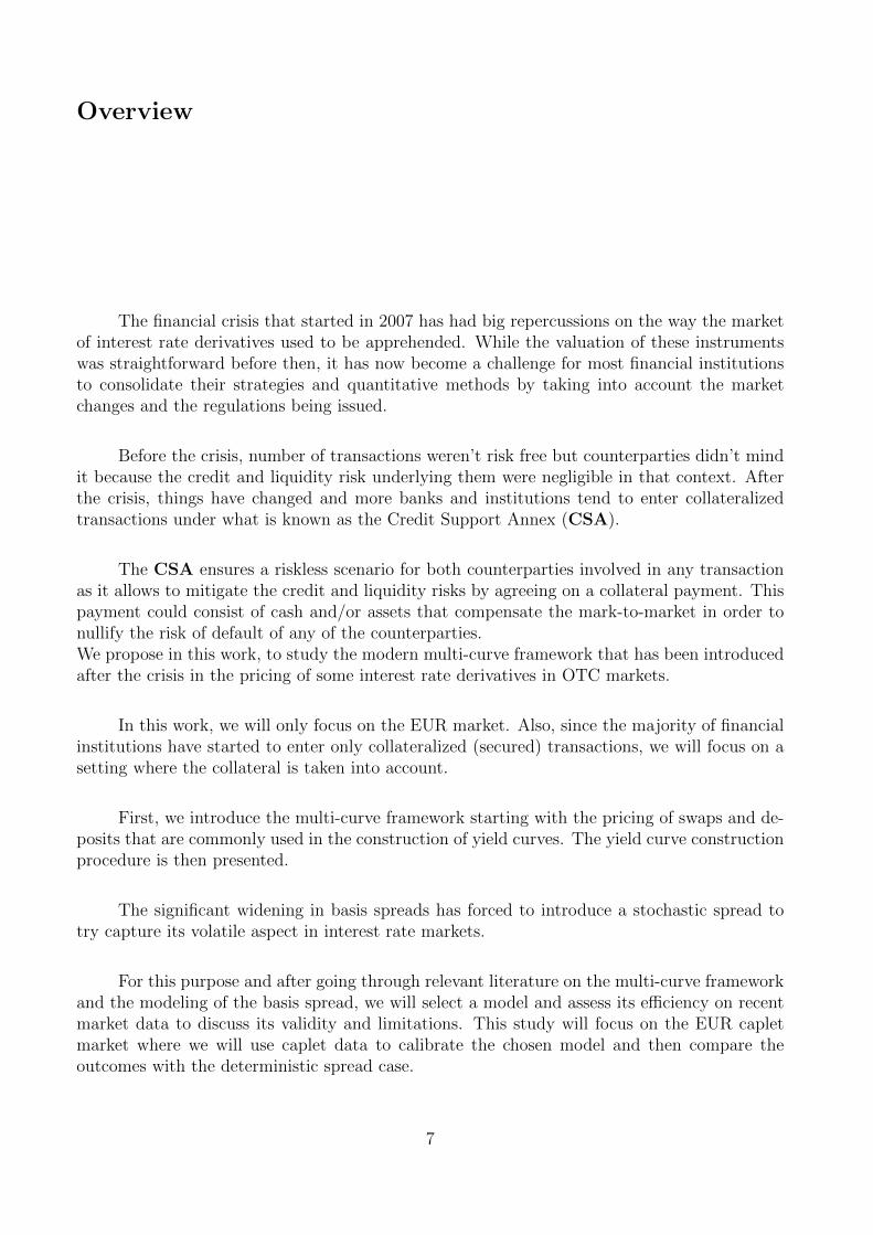
The financial crisis that started in 2007 has had big repercussions on the way the marketof interest rate derivatives used to be apprehended. While the valuation of these instrumentswas straightforward before then, it has now become a challenge for most financial institutionsto consolidate their strategies and quantitative methods by taking into account the marketchanges and the regulations being issued.

Before the crisis, number of transactions weren’t risk free but counterparties didn’t mindit because the credit and liquidity risk underlying them were negligible in that context. Afterthe crisis, things have changed and more banks and institutions tend to enter collateralizedtransactions under what is known as the Credit Support Annex (CSA).

The CSA ensures a riskless scenario for both counterparties involved in any transactionas it allows to mitigate the credit and liquidity risks by agreeing on a collateral payment. Thispayment could consist of cash and/or assets that compensate the mark-to-market in order tonullify the risk of default of any of the counterparties.We propose in this work, to study the modern multi-curve framework that has been introducedafter the crisis in the pricing of some interest rate derivatives in OTC markets.

In this work, we will only focus on the EUR market. Also, since the majority of financialinstitutions have started to enter only collateralized (secured) transactions, we will focus on asetting where the collateral is taken into account.

First, we introduce the multi-curve framework starting with the pricing of swaps and de-posits that are commonly used in the construction of yield curves. The yield curve constructionprocedure is then presented.

The significant widening in basis spreads has forced to introduce a stochastic spread totry capture its volatile aspect in interest rate markets.

For this purpose and after going through relevant literature on the multi-curve frameworkand the modeling of the basis spread, we will select a model and assess its efficiency on recentmarket data to discuss its validity and limitations. This study will focus on the EUR capletmarket where we will use caplet data to calibrate the chosen model and then compare theoutcomes with the deterministic spread case.

7

Definitions and Key Words

Abbreviations and Key Words:

CDS Credit Default SwapCSA Credit Support Annex

D DayDCL Dexia Credit Local

EONIA Euro OverNight Index AverageIRS Interest Rate Swap(s)M Month

mkt MarketNPV Net Present ValueOIS Overnight Index Swap(s)ON Over Night

OTC Over-The-CounterSABR Stochastic Alpha Beta Rho

W WeekXIBOR X InterBank Offered Rate (X = LIBOR, EURO, ...)

Y Year

Definitions:

In this section, we define some notions that are going to be used throughout thisreport. Other notions will be defined when used.

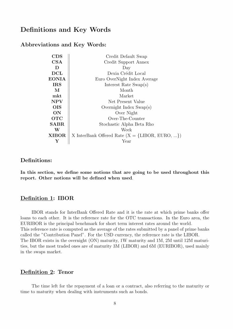
Definition 1: IBOR

IBOR stands for InterBank Offered Rate and it is the rate at which prime banks offerloans to each other. It is the reference rate for the OTC transactions. In the Euro area, theEURIBOR is the principal benchmark for short term interest rates around the world.This reference rate is computed as the average of the rates submitted by a panel of prime bankscalled the ”Contribution Panel”. For the USD currency, the reference rate is the LIBOR.The IBOR exists in the overnight (ON) maturity, 1W maturity and 1M, 2M until 12M maturi-ties, but the most traded ones are of maturity 3M (LIBOR) and 6M (EURIBOR), used mainlyin the swaps market.

Definition 2: Tenor

The time left for the repayment of a loan or a contract, also referring to the maturity ortime to maturity when dealing with instruments such as bonds.

8

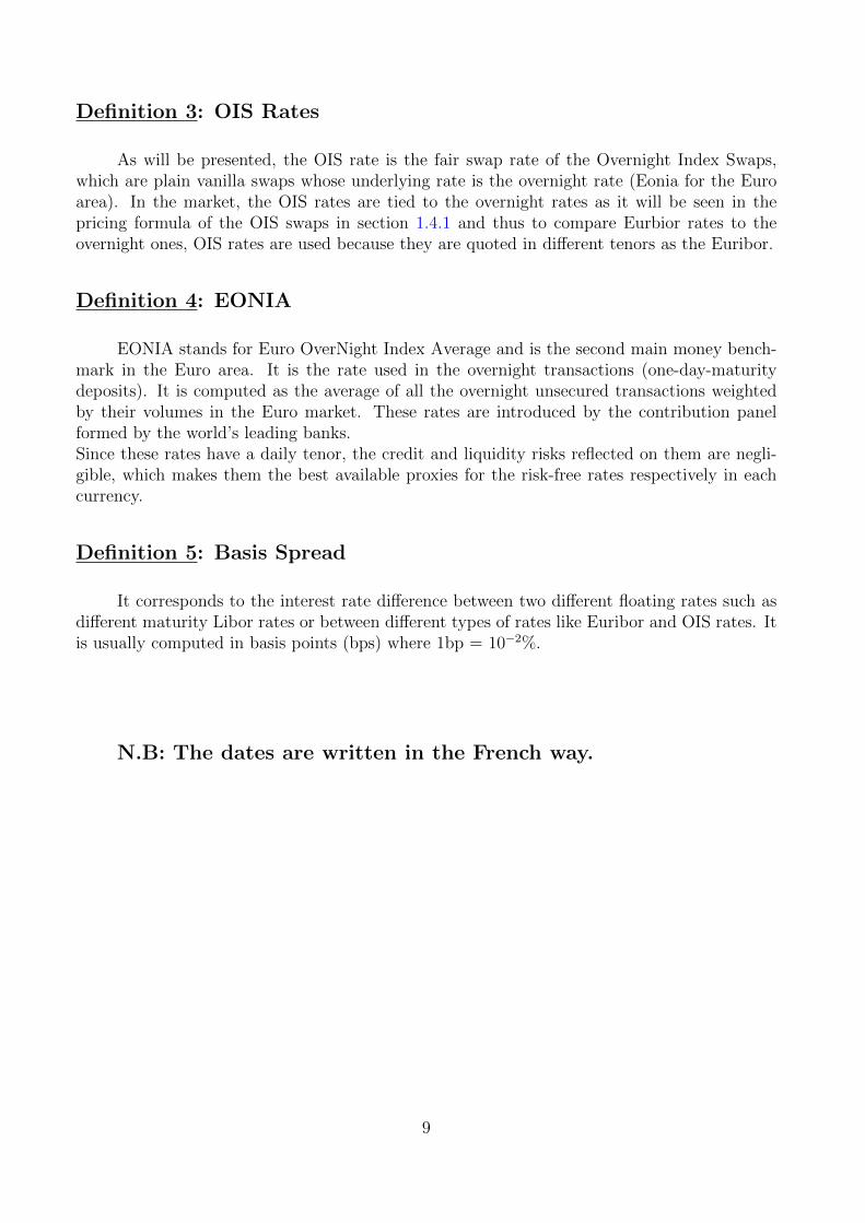
Definition 3: OIS Rates

As will be presented, the OIS rate is the fair swap rate of the Overnight Index Swaps,which are plain vanilla swaps whose underlying rate is the overnight rate (Eonia for the Euroarea). In the market, the OIS rates are tied to the overnight rates as it will be seen in thepricing formula of the OIS swaps in section 1.4.1 and thus to compare Eurbior rates to theovernight ones, OIS rates are used because they are quoted in different tenors as the Euribor.

Definition 4: EONIA

EONIA stands for Euro OverNight Index Average and is the second main money bench-mark in the Euro area. It is the rate used in the overnight transactions (one-day-maturitydeposits). It is computed as the average of all the overnight unsecured transactions weightedby their volumes in the Euro market. These rates are introduced by the contribution panelformed by the world’s leading banks.Since these rates have a daily tenor, the credit and liquidity risks reflected on them are negli-gible, which makes them the best available proxies for the risk-free rates respectively in eachcurrency.

Definition 5: Basis Spread

It corresponds to the interest rate difference between two different floating rates such asdifferent maturity Libor rates or between different types of rates like Euribor and OIS rates. Itis usually computed in basis points (bps) where 1bp = 10−2%.

N.B: The dates are written in the French way.

9

Goals and Recurrent Notations

The aim of my master thesis is to perform the pricing of some plain vanilla interest ratederivatives (deposits, swaps and caplets) in the multi-curve framework after constructing theyield curves properly, then study models for a stochastic basis spread and choose one specificmodel to implement in the pricing library of the DCL and assess its efficiency in generatingprices that are consistent with the market. I have divided the work into subtasks as follows:

1. Explore the literature on the multi-curve framework,

2. Implement the pricing of plain vanilla interest rate swaps and basis swaps in the multi-curve setting,

3. Propose a model for a stochastic basis spread and implement it,

4. Perform the pricing of plain vanilla interest rate caplets and compare the results withmarket data,

5. Conclude on the validity and accuracy of the model and discuss its outcomes and eventuallimitations.

In addition to the notations that are going to be explained throughout the report, we willuse the following ones recurrently:

• Px(t, T ) is the discount factor (the zero coupon price at time t) taken from the curve Cx,which is whether the discount curve Cd or the forward curve Cm.

Px(t, T ) = EQt [e−∫ Tt rxdx],

where Q is the risk neutral measure and rx is the short rate.

• Ft to designate the natural filtration associated to a stochastic process. It is mainly usedin the no-arbitrage pricing formula, in the conditional expectations, and we will, fromnow on, use Ft for every stochastic process, for simplicity, but it doesn’t mean that itis the same filtration for all of them. It represents the information generated by thecorresponding process up until time t.

• EQTx

t to designate the conditional expectation EQTx [.|Ft] taken under the measure QTx ,

which is defined when considering T → Px(t, T ) to be the numeraire. In thisreport x will designate d for the discount curve and m for the forward curve of tenor m.

• γm(Ti−1, Ti) is the year fraction corresponding to the period [Tmi−1, Tmi ] for a term structure

that is homogeneous with a tenor m, i.e. Tmi−1 − Tmi = m.

10

1 The Multi-Curve Framework

The OTC interest rate derivatives market has for a long time been mastered before thefinancial crisis of 2007, in terms of valuation. Not only has the crisis brought about a drasticchange in the behaviour of interest rates, particularly the Libor rate, but it also has forcedpractitioners to rethink their evaluation strategies.

The multi-curve paradigm has since then been incorporated and is now adopted as themodern framework.

Our aim in this section is to emphasize this transition as well as its whys and wherefores.

1.1 Interest Rate Spread Increase

Before the financial crisis, the interest rates were mutually consistent, meaning, their dif-ferences were considered negligible as their spreads were very small in terms of basis points.

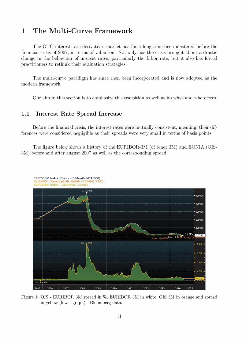
The figure below shows a history of the EURIBOR-3M (of tenor 3M) and EONIA (OIS-3M) before and after august 2007 as well as the corresponding spread.

Figure 1: OIS - EURIBOR 3M spread in %, EURIBOR 3M in white, OIS 3M in orange and spreadin yellow (lower graph) - Bloomberg data.

11

The rates and spread are quoted in percent.

Before the third quarter of 2007, the two rates were matching almost perfectly as theirspread hovered around 0.We observe an obvious increase of the spread from the third quarter of 2007 (August 2007)from −1.6 bps (-0.016 %: the spread was exceptionally negative at one date at the end of 2005,but always positive since then) to 195.5 bps (1.955 %) in October 2008 and then stabilizesfrom then up until the second quarter of 2011. The peak in 2008 is mainly due to the LehmanBrothers collapse.The end of 2011 was characterized by a new explosion of the EURIBOR 3M - OIS 3M spreaddue to the interest rate remarkable decrease especially in the greek market.From the third quarter of 2012 until now, the spread seemed to have stabilized again at around10 bps.

This spread explosion is a consequence of the difference in the credit and liquidity riskintrinsic to both Euribor and Eonia rates.As a matter of fact, the level of credit and liquidity risk in the Euribor rate is higher thanin Eonia. Eonia being an overnight rate calculated from the overnight transactions, it has alow level of risk, because these transactions can be considered risk-free as changes during anovernight period are relatively weak, and the probability of default of one of the counterparties(or both) engaged in such transactions tends to zero.That’s why OIS rates are considered to be the best proxies for risk-free rates, for the timebeing.On the other side, the credit and liquidity risk components of the Ibor (in general) have in-creased during the crisis, which was also observable throught the explosion of the Credit DefaultSwaps (CDS) describing a general increase in the default risk (credit crunch). These CDS swapsallowed counterparties to protect themselves from the default of their counterparties.

The reason the spread increased is that banks among other institutions started having lessconfidence in proposing loans to each other as some of them became less creditworthy, whichhas led them to increase their loan interest rates amongst which, the Libor.

To understand this, we present a scenario where a bank A sells a bond to bank B. Thebond has a probability p of defaulting. Bank B enters a CDS (buys the CDS from A) withbank A, which insures for B to receive the face value of the bond from A in case of default inexchange for the bond, which is worthless for B (see figure 2). The CDS, in case of default,pays the face value of the bond to B and nothing if no default occurs.

12

Figure 2: Up: Scenario of a bond exchange between A (seller) and B (buyer), where B also buys aCDS from A to protect itself from an eventual default.Down: Scenario of a bond exchange between A (seller) and B (buyer), without CDS.Red arrows correspond to the event of default (probability p) and the blue ones to the eventof non default (probability 1− p).

In our example, the bank giving the loan is bank B (B buys the bond by paying an amountwhich is equivalent to the loan at first and receiving interests), so if A defaults (or if the bonddefaults), B won’t receive its interest payments and thus will lose out of this transaction. If Benters a CDS with A then it can protect itself from A’s default. This scenario was commonduring the period of the crisis and CDS swaps increased remarkably, expressing the low levelof confidence between counterparties. As a consequence loans’ interest rates increased as wellto try compensate the high risk of default.

1.2 Market Segmentation

The divergence of the interest rate have led to a segmentation of the market into sub-areas corresponding to interest rates of different tenors. The value of the spread after the crisisdoesn’t allow to consider using a unique yield curve indifferently for all tenors as a correctpractice.

As a matter of fact the idea of assigning a distinct yield curve to each different tenorhappened to be wiser and more realistic according to the current context of the market.Before this segmentation, the pricing of interest rate derivatives only needed one unique curveboth for computing the forward rates and the discount factors used in the computation of thenet present value (NPV) of the cash flows generated by the derivative of interest. This formerly

13

common practice cannot be used anymore due to the inconsistencies between interest rates andthe fact that the pricing formulae should take the market segmentation into account.

The latter is what led to introduce the multi-curve framework.

Now, it is crucial to build one curve for the discounting of the future cash flows anddistinct curves corresponding to the different tenors used for computing the forward rates.From now on, the discounting curve and the forwarding (also called fixing or funding) curveswill be noted Cd and Cm respectively, where m ∈ m1,m2, ...,mk the different relevant tenors.

Before we get to the curve construction, we start by introducing the multi-curve frame-work and the modifications it brings to the pricing of interest rate derivatives.

1.3 Pricing of Interest Rate Derivatives in the Multi-Curve Frame-work

Recall that the principle of the multi-curve framework is to define a unique curve dedi-cated to discounting the future cash flows of a derivative and multiple curves for funding, eachcorresponding to a different rate tenor. Let’s start by presenting the fundamental quantity ofthe multi-curve setting.

1.3.1 The FRA rate

The FRA rate is the rate of a Forward Rate Agreement, which is a contract between twocounterparties in which they agree on applying a certain rate during a certain period of timestarting from a predetermined date in the future.Let T1 and T2 define a future period [T1, T2] and t be the present date. The FRA rate,FRA(t;T1, T2), can be seen as the fixed rate to be exchanged at T2 for the Libor rate L(T1, T2)so that the t-value of the corresponding ”one cash flow” swap is zero.

Denote by ΦSwap(t) the t-price of this swap. Under the QT2d measure (whose numeraire is

Pd(t, T2) the discount factor from t to T2 related to the discount curve) the process ΦSwap(t)/Pd(t, T2)is a martingale, so the condition above is expressed by:

ΦSwap(t)

Pd(t, T2)= EQ

T2d

t

[ΦSwap(T2)

Pd(T2, T2)

]= 0

where ΦSwap(T2) is the payoff of the swap at T2 i.e. ΦSwap(T2) = Nω(L(T1, T2)−FRA(t;T1, T2))and Pd(T2, T2) = 1.So

NωEQT2d

t [L(T1, T2)− FRA(t;T1, T2)] = 0,where N is the notional amount of the swap and ω = ±1 depending on the counterparty side.

14

or

EQT2d

t [L(T1, T2)]− EQT2d

t [FRA(t;T1, T2)] = 0,and since FRA(t;T1, T2) is known at time t, it is then Ft-measurable so,

FRA(t;T1, T2) = EQT2d

t [L(T1, T2)] .

The Libor rate L(T1, T2) is defined by:

L(T1, T2) =1

T2 − T1

(1

Pd(T1, T2)− 1

). (1)

In the single-curve framework where only one curve was used for all purposes (discounting

and funding), the forward rate Fd(t;T1, T2) = 1T2−T1

(Pd(t,T1)Pd(t,T2)

− 1)

corresponding to the period

[T1, T2] used to coincide with the FRA rate FRA(t;T1, T2) because:

FRA(t;T1, T2) = EQT2d

t [L(T1, T2)] = EQT2d

t [Fd(T1;T1, T2)] = Fd(t;T1, T2),since Fd(t;T1, T2) is a martingale under QT2

d .

In the multi-curve framework L(T1, T2) 6= Fd(T1;T1, T2) since the discount factors in (1)are not the ones corresponding to the discount curve. The discount factors to be used will nowdepend on the underlying tenor of the Libor and thus the fixings will be calculated from thecorresponding forward curve and not from the discount one.

In this new framework, the equality FRA(t;T1, T2) = Fd(t;T1, T2) won’t hold anymorebut a spread appears between the two quantities.

Furthermore we have:

EQT2d

t [FRA(T1;T1, T2)] = EQT2d

t

[EQ

T2d [L(T1, T2)|FT1 ]

]and since L(T1, T2) is known at time T1 then

EQT2d

t [FRA(T1;T1, T2)] = EQT2d

t [L(T1, T2)] = FRA(t;T1, T2).This means that under QT2

d , FRA(t;T1, T2) is a martingale.This is an important result that will be of precious use in the pricing of interest rate derivativesin the multi-curve framework.

1.3.2 The No-Arbitrage Pricing Formula

We have just shown that the FRA rate is a martingale under the forward measure.Let Φ(T ) the payoff of an interest rate derivative at a maturity time T . The arbitrage-free priceof the derivative at time t is given by:

Φ(t) = Pd(t, T )EQTd

t [Φ(T )], (2)

where Pd(t, T ) = EQt [e−∫ Tt rudu] (Q is the risk-neutral measure) and Pd(t, T ) = e−

∫ Tt rudu if the

short collateral rate ru is deterministic.

The payoff Φ(T ) is generally a function of the Libor rate L, so the expectation of theLibor rate will lead to the appearance of the FRA rate in the pricing formula.

We consider the collateral rate to be the OIS rate when dealing with collat-eralized instruments, so the discounting will be performed using the OIS discount

curve: Pd(t, T ) = e−∫ Tt rOIS(u)du.

15

1.3.3 Pricing Formulae for Plain Vanilla Instruments

In this section, we derive the pricing formulae for the plain vanilla interest rate deriva-tives used in the construction of yield curves in the multi-curve framework, namely depositsand swaps.

Remark:Nowadays, the instruments traded in the market are mostly collateralized, meaningthat the transaction between two counterparties is written under collateral agree-ment (CSA) as explained in the ”Overview”. For that purpose, the discounting ismostly performed using the OIS curve whose construction is explained in section1.4.1. Our aim is not to discuss the collateral management, that is why we positionourselves in a market where all trades are made under perfect collateral (Section(1.4.1)).

• Deposits:

A deposit is a zero coupon contract where a counterparty A (lender) lends a nominal Nat T0 to a counterparty B (borrower), which at maturity T, pays the notional amountback to the lender as well as the interest accrued over the period [T0, T ] at a simplycompounded rate Rm(T0, T ) fixed at a date TF ≤ T0 and of tenor m corresponding to thetime interval [T0, T ] (i.e. m = T − T0).Remark: A deposit is not a collateralized contract, so the discounting doesn’t involvethe OIS curve and instead uses the forward curve of tenor m.

The payoff of the deposit at maturity T from the lender’s point view is given by:ΦDeposit(T ) = N(1 +Rm(T0, T )γ(T0, T )),

where γ(T0, T ) is the day count fraction corresponding to the period [T0, T ].The price at a time t ∈ [TF , T ] is obtained by using the no-arbitrage argument and thefact that under the probability measure QT

m whose numeraire is Pm(t, T ) (discount factor

based on the same rate tenor m as the deposit rate’s), the process ΦDeposit(t)

Pm(t,T ) is a mar-

tingale. So:

ΦDeposit(t)

Pm(t, T )= EQ

Tm

t

[ΦDeposit(T )

Pm(T, T )

]and because the rateRm is already fixed and known at time t, ΦDeposit(T ) is Ft−measurableso

ΦDeposit(t) = Pm(t, T )EQTm

t [ΦDeposit(T )] = NPm(t, T )(1 +Rm(T0, T )γ(T0, T )).Moreover, as the initial amount invested in the deposit is N, by no-arbitrage agrument,the following relation holds:

ΦDeposit(t) = N = NPm(t, T )(1 +Rm(T0, T )γ(T0, T )). (3)

16

• Interest Rate Swaps (IRS):

A swap is a contract where two counterparties agree to exchange two sets of cash flows(generated by two legs) in the same currency, typically one of the two legs is indexed (tiedto) a floating rate, particularly Euribor and the second one is a fixed rate K determinedat the agreement date.Let ΩT = T0, T1, ..., Tn be the cash flow schedule of the floating leg and ΩS = S0, S1, ..., Sn′that of the fixed leg (with rate K), where S0 = T0 is the settlement date of the contractand also the date where the first Euribor rate Lm(T0, T1) (m is the tenor of the underlyingEuribor) is fixed but payed only at T1. n and n′ are the numbers of floating and fixedpayments of the swap, respectively.Figure (3) shows the swap cash flow diagram:

Floating Leg (ΩT )

T0 = S0t T1 T2 T3 Tn...

Lm(T0, T1) Lm(T1, T2) Lm(T2, T3) Lm(Tn−1, Tn)

Fixed Leg (ΩS)

t S0 S1 S2 S3 Sn′...

K K K K

Figure 3: IRS cash flow diagram.

The price of the IRS at t, T0 ≤ t ≤ T (T is the maturity of the swap) is given by (ref.equation (2)):

ΦIRS(t) = Nω

[n∑i=1

Pd(t, Ti)γfloat(Ti−1, Ti)EQTid

t [Lm(Ti−1, Ti)]−n′∑j=1

KPd(t, Sj)γK(Sj−1, Sj)

]Where each payment of each leg is discounted at time t. So

ΦIRS(t) = Nω [RIRS(t,ΩT ,ΩS)−K]Ad(t,ΩS), (4)where

RIRS(t,ΩT ,ΩS) =

∑ni=1 Pd(t, Ti)FRAm(t, Ti−1, Ti)γfloat(Ti−1, Ti)

Ad(t,ΩS), (5)

Ad(t,ΩS) =n′∑j=1

Pd(t, Sj)γK(Sj−1, Sj),

Here Pd(t, Ti) is the discount factor.N is the notional, ω = 1 if the fixed leg is payed and ω = −1 if the floating leg is payed,

FRAm(t, Ti−1, Ti) = EQTid

t [Lm(Ti−1, Ti)] is the FRA rate of tenor m corresponding to[Ti−1, Ti], γfloat(Ti−1, Ti) and γK(Sj−1, Sj) are the year fractions corresponding to the float-ing and fixed payment periods [Ti−1, Ti] (i ∈ 0, 1, ..., n) and [Sj−1, Sj] (j ∈ 0, 1, ..., n′),respectively.

Remark: The calculation of the discount factors Pd appearing in the formulae aboveis explained in the following section.

17

1.4 Curve Construction in the Multi-Curve Framework

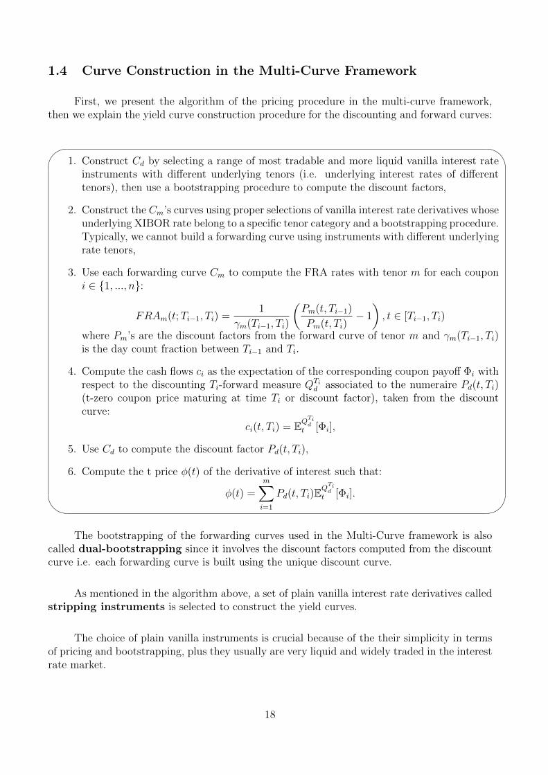
First, we present the algorithm of the pricing procedure in the multi-curve framework,then we explain the yield curve construction procedure for the discounting and forward curves:

'

&

$

%

1. Construct Cd by selecting a range of most tradable and more liquid vanilla interest rateinstruments with different underlying tenors (i.e. underlying interest rates of differenttenors), then use a bootstrapping procedure to compute the discount factors,

2. Construct the Cm’s curves using proper selections of vanilla interest rate derivatives whoseunderlying XIBOR rate belong to a specific tenor category and a bootstrapping procedure.Typically, we cannot build a forwarding curve using instruments with different underlyingrate tenors,

3. Use each forwarding curve Cm to compute the FRA rates with tenor m for each couponi ∈ 1, ..., n:

FRAm(t;Ti−1, Ti) =1

γm(Ti−1, Ti)

(Pm(t, Ti−1)

Pm(t, Ti)− 1

), t ∈ [Ti−1, Ti)

where Pm’s are the discount factors from the forward curve of tenor m and γm(Ti−1, Ti)is the day count fraction between Ti−1 and Ti.

4. Compute the cash flows ci as the expectation of the corresponding coupon payoff Φi withrespect to the discounting Ti-forward measure QTi

d associated to the numeraire Pd(t, Ti)(t-zero coupon price maturing at time Ti or discount factor), taken from the discountcurve:

ci(t, Ti) = EQTid

t [Φi],

5. Use Cd to compute the discount factor Pd(t, Ti),

6. Compute the t price φ(t) of the derivative of interest such that:

φ(t) =m∑i=1

Pd(t, Ti)EQTid

t [Φi].

The bootstrapping of the forwarding curves used in the Multi-Curve framework is alsocalled dual-bootstrapping since it involves the discount factors computed from the discountcurve i.e. each forwarding curve is built using the unique discount curve.

As mentioned in the algorithm above, a set of plain vanilla interest rate derivatives calledstripping instruments is selected to construct the yield curves.

The choice of plain vanilla instruments is crucial because of the their simplicity in termsof pricing and bootstrapping, plus they usually are very liquid and widely traded in the interestrate market.

18

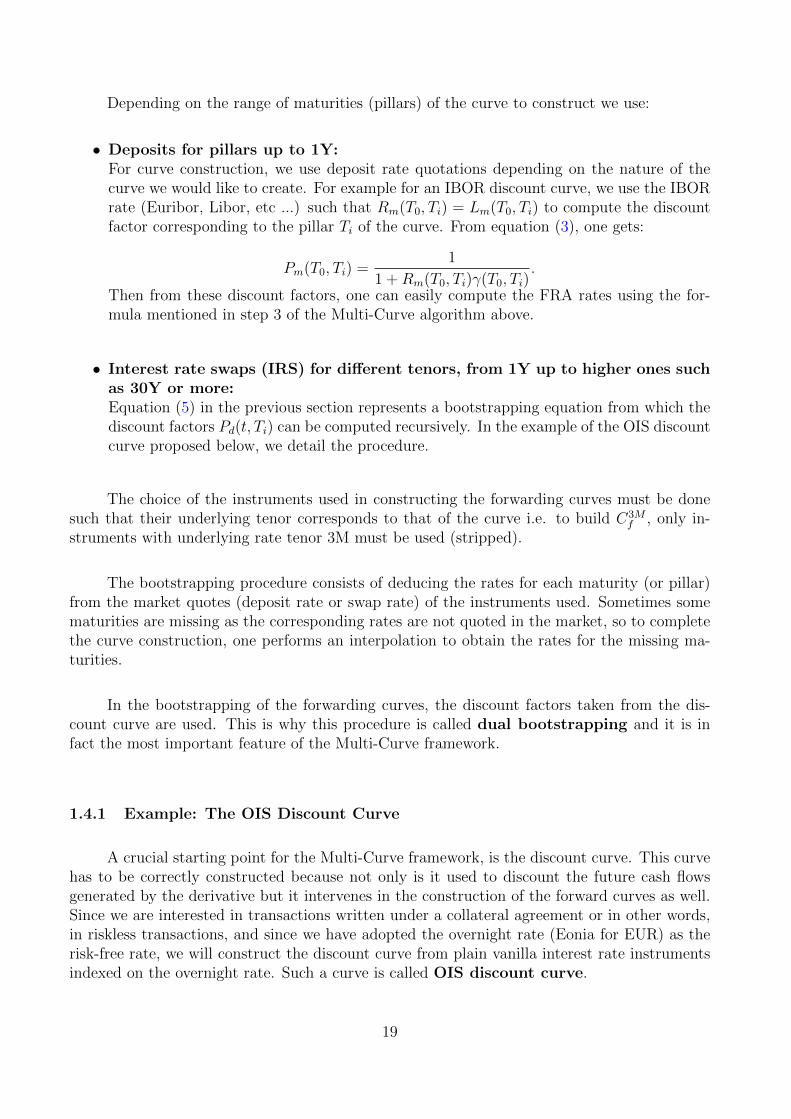
Depending on the range of maturities (pillars) of the curve to construct we use:

• Deposits for pillars up to 1Y:For curve construction, we use deposit rate quotations depending on the nature of thecurve we would like to create. For example for an IBOR discount curve, we use the IBORrate (Euribor, Libor, etc ...) such that Rm(T0, Ti) = Lm(T0, Ti) to compute the discountfactor corresponding to the pillar Ti of the curve. From equation (3), one gets:

Pm(T0, Ti) =1

1 +Rm(T0, Ti)γ(T0, Ti).

Then from these discount factors, one can easily compute the FRA rates using the for-mula mentioned in step 3 of the Multi-Curve algorithm above.

• Interest rate swaps (IRS) for different tenors, from 1Y up to higher ones suchas 30Y or more:Equation (5) in the previous section represents a bootstrapping equation from which thediscount factors Pd(t, Ti) can be computed recursively. In the example of the OIS discountcurve proposed below, we detail the procedure.

The choice of the instruments used in constructing the forwarding curves must be donesuch that their underlying tenor corresponds to that of the curve i.e. to build C3M

f , only in-struments with underlying rate tenor 3M must be used (stripped).

The bootstrapping procedure consists of deducing the rates for each maturity (or pillar)from the market quotes (deposit rate or swap rate) of the instruments used. Sometimes somematurities are missing as the corresponding rates are not quoted in the market, so to completethe curve construction, one performs an interpolation to obtain the rates for the missing ma-turities.

In the bootstrapping of the forwarding curves, the discount factors taken from the dis-count curve are used. This is why this procedure is called dual bootstrapping and it is infact the most important feature of the Multi-Curve framework.

1.4.1 Example: The OIS Discount Curve

A crucial starting point for the Multi-Curve framework, is the discount curve. This curvehas to be correctly constructed because not only is it used to discount the future cash flowsgenerated by the derivative but it intervenes in the construction of the forward curves as well.Since we are interested in transactions written under a collateral agreement or in other words,in riskless transactions, and since we have adopted the overnight rate (Eonia for EUR) as therisk-free rate, we will construct the discount curve from plain vanilla interest rate instrumentsindexed on the overnight rate. Such a curve is called OIS discount curve.

19

The principal instrument used for the bootstrapping of the OIS discount curve is the”Overnight Index Swap”.The OIS is a plain vanilla interest rate swap exchanging a fixed rate and the daily compoundedovernight rate. Let ΩT = T0, T1, ..., Tn be the cash flow schedule of the floating leg andΩS = S0, S1, ..., Sn′ that of the fixed rate K, where S0 = T0 is the settlement date of thecontract. The frequency of the floating leg is not daily but is considered to be the same as thefrequency of the fixed leg. n and n′ are the numbers of floating and fixed payments of the OIS,respectively.The schedule of the floating leg is decomposed into daily periods i.e.

[Ti−1, Ti] =ni∪k=1

(Ti,k−1, Ti,k],

where ni is the number of daily overnight payments in the period [Ti−1, Ti]. Let RON(Ti,Ti)(Ti = Ti,0, ..., Ti,ni the overnight payment schedule for the i-th period) be the coupon ratecompounded from overnight rates over the i-th period [Ti−1, Ti].Figure 4 displays the diagram of the OIS cash flows.

Floating Leg (ΩT )

T0 = S0t T1 T2 T3 TnT2,1 T2,2...T2,n2−1 ...

RON(T1,T1) RON(T2,T2) RON(T3,T3) RON(Tn,Tn)

Fixed Leg (ΩS)

t S0 S1 S2 S3 Sn′...

K K K K

Figure 4: OIS cash flow diagram.

We have:

1 +RON(Ti,Ti)γON(Ti−1, Ti) =

ni∏k=1

[1 +RON(Ti,k−1, Ti,k)γON(Ti,k−1, Ti,k)],

or

RON(Ti,Ti) =1

γON(Ti−1, Ti)

ni∏k=1

[1 +RON(Ti,k−1, Ti,k)γON(Ti,k−1, Ti,k)]− 1

The OIS price (supposing the fixed leg being payed) at t, T0 ≤ t ≤ TOIS (TOIS is the maturityof the OIS) is given by:

ΦOIS(t) = Nω(ROIS(t,ΩT ,ΩS)−K

)Ac(t,ΩS),

where

ROIS(t,ΩT ,ΩS) =

∑ni=1 Pc(t, Ti)RON(t,Ti)γON(Ti−1, Ti)

Ac(t,ΩS), (6)

Ac(t,ΩS) =n′∑j=1

Pc(t, Sj)γK(Sj−1, Sj),

20

Here Pc(t, Ti) is the discount factor under collateral using the risk free Eonia rate.N is the notional in EUR (for an OIS on underlying Eonia), RON(t,Ti) is the FRA overnightrate Eonia corresponding to the i-th period [Ti−1, Ti], γON(Ti−1, Ti) and γK(Sj−1, Sj) are the yearfractions corresponding to the floating and fixed payment periods [Ti−1, Ti] (i ∈ 0, 1, ..., n)and [Sj−1, Sj] (j ∈ 0, 1, ..., n′), respectively.

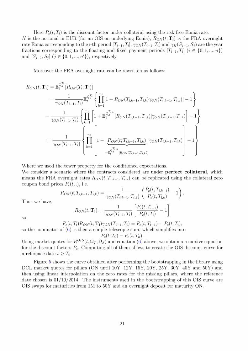
Moreover the FRA overnight rate can be rewritten as follows:

RON(t,Ti) = EQTid

t [RON(Ti,Ti)]

=1

γON(Ti−1, Ti)EQ

Tid

t

ni∏k=1

[1 +RON(Ti,k−1, Ti,k)γON(Ti,k−1, Ti,k)]− 1

=1

γON(Ti−1, Ti)

ni∏k=1

[1 + EQ

Ti,kd

t [RON(Ti,k−1, Ti,k)]γON(Ti,k−1, Ti,k)

]− 1

=1

γON(Ti−1, Ti)

ni∏k=1

1 + RON(t;Ti,k−1, Ti,k)︸ ︷︷ ︸=E

QTi,kd

t [RON (Ti,k−1,Ti,k)]

γON(Ti,k−1, Ti,k)

− 1

Where we used the tower property for the conditioned expectations.We consider a scenario where the contracts considered are under perfect collateral, whichmeans the FRA overnight rates RON(t, Ti,k−1, Ti,k) can be replicated using the collateral zerocoupon bond prices Pc(t, .), i.e.

RON(t, Ti,k−1, Ti,k) =1

γON(Ti,k−1, Ti,k)

(Pc(t, Ti,k−1)

Pc(t, Ti,k)− 1

).

Thus we have,

RON(t,Ti) =1

γON(Ti−1, Ti)

[Pc(t, Ti−1)

Pc(t, Ti)− 1

]so

Pc(t, Ti)RON(t,Ti)γON(Ti−1, Ti) = Pc(t, Ti−1)− Pc(t, Ti),so the nominator of (6) is then a simple telescopic sum, which simplifies into

Pc(t, T0)− Pc(t, Tn).Using market quotes for ROIS(t,ΩT ,ΩS) and equation (6) above, we obtain a recursive equationfor the discount factors Pc. Computing all of them allows to create the OIS discount curve fora reference date t ≥ T0.

Figure 5 shows the curve obtained after performing the bootstrapping in the library usingDCL market quotes for pillars (ON until 10Y, 12Y, 15Y, 20Y, 25Y, 30Y, 40Y and 50Y) andthen using linear interpolation on the zero rates for the missing pillars, where the referencedate chosen is 01/10/2014. The instruments used in the bootstrapping of this OIS curve areOIS swaps for maturities from 1M to 50Y and an overnight deposit for maturity ON.

21

Figure 5: Up: OIS discount curve as of 01/10/2014, linear interpolation on the zero rates, down:Quoted interest rates.

22

1.4.2 Example: Pricing of an IRS in the Multi-Curve Setting

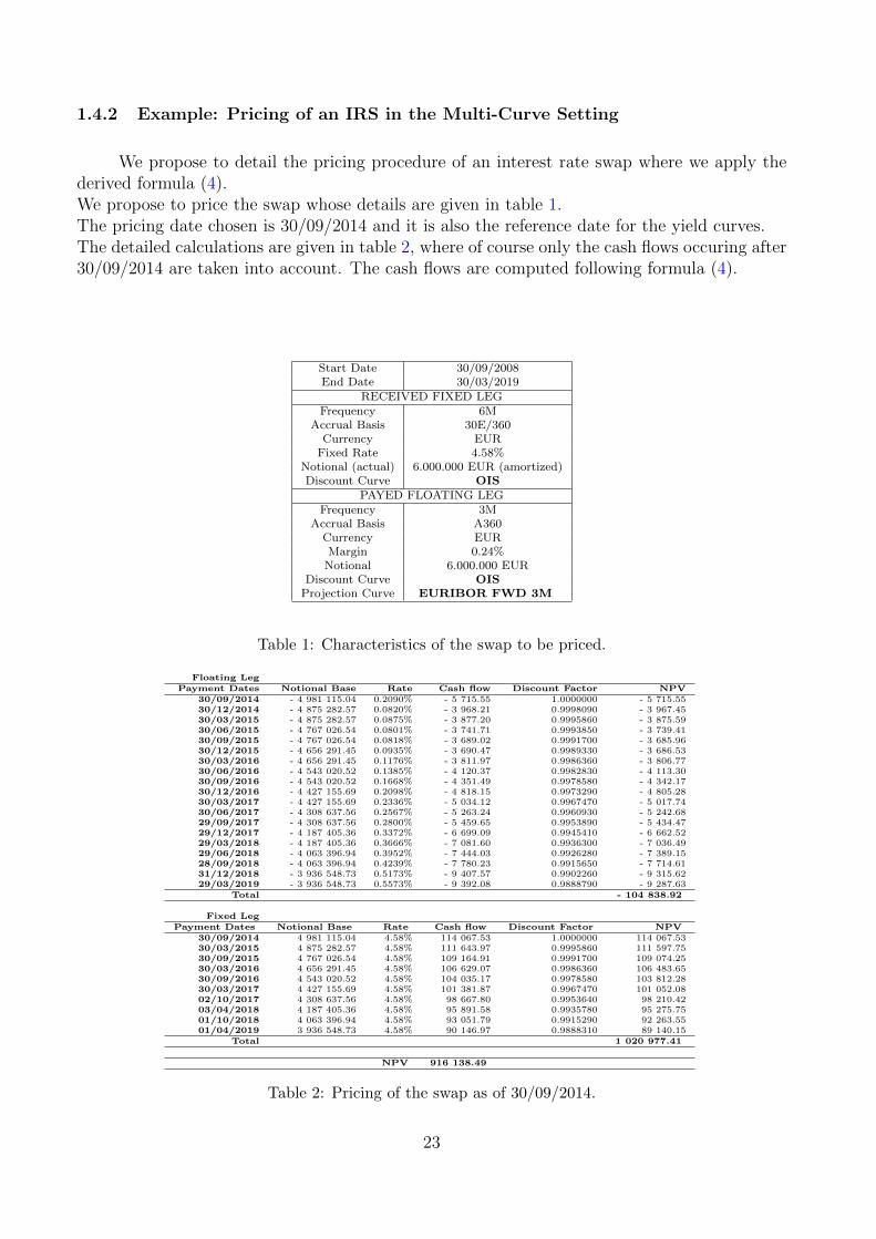
We propose to detail the pricing procedure of an interest rate swap where we apply thederived formula (4).We propose to price the swap whose details are given in table 1.The pricing date chosen is 30/09/2014 and it is also the reference date for the yield curves.The detailed calculations are given in table 2, where of course only the cash flows occuring after30/09/2014 are taken into account. The cash flows are computed following formula (4).

Start Date 30/09/2008End Date 30/03/2019

RECEIVED FIXED LEGFrequency 6M

Accrual Basis 30E/360Currency EUR

Fixed Rate 4.58%Notional (actual) 6.000.000 EUR (amortized)Discount Curve OIS

PAYED FLOATING LEGFrequency 3M

Accrual Basis A360Currency EURMargin 0.24%

Notional 6.000.000 EURDiscount Curve OIS

Projection Curve EURIBOR FWD 3M

Table 1: Characteristics of the swap to be priced.

Floating LegPayment Dates Notional Base Rate Cash flow Discount Factor NPV

30/09/2014 - 4 981 115.04 0.2090% - 5 715.55 1.0000000 - 5 715.5530/12/2014 - 4 875 282.57 0.0820% - 3 968.21 0.9998090 - 3 967.4530/03/2015 - 4 875 282.57 0.0875% - 3 877.20 0.9995860 - 3 875.5930/06/2015 - 4 767 026.54 0.0801% - 3 741.71 0.9993850 - 3 739.4130/09/2015 - 4 767 026.54 0.0818% - 3 689.02 0.9991700 - 3 685.9630/12/2015 - 4 656 291.45 0.0935% - 3 690.47 0.9989330 - 3 686.5330/03/2016 - 4 656 291.45 0.1176% - 3 811.97 0.9986360 - 3 806.7730/06/2016 - 4 543 020.52 0.1385% - 4 120.37 0.9982830 - 4 113.3030/09/2016 - 4 543 020.52 0.1668% - 4 351.49 0.9978580 - 4 342.1730/12/2016 - 4 427 155.69 0.2098% - 4 818.15 0.9973290 - 4 805.2830/03/2017 - 4 427 155.69 0.2336% - 5 034.12 0.9967470 - 5 017.7430/06/2017 - 4 308 637.56 0.2567% - 5 263.24 0.9960930 - 5 242.6829/09/2017 - 4 308 637.56 0.2800% - 5 459.65 0.9953890 - 5 434.4729/12/2017 - 4 187 405.36 0.3372% - 6 699.09 0.9945410 - 6 662.5229/03/2018 - 4 187 405.36 0.3666% - 7 081.60 0.9936300 - 7 036.4929/06/2018 - 4 063 396.94 0.3952% - 7 444.03 0.9926280 - 7 389.1528/09/2018 - 4 063 396.94 0.4239% - 7 780.23 0.9915650 - 7 714.6131/12/2018 - 3 936 548.73 0.5173% - 9 407.57 0.9902260 - 9 315.6229/03/2019 - 3 936 548.73 0.5573% - 9 392.08 0.9888790 - 9 287.63

Total - 104 838.92

Fixed LegPayment Dates Notional Base Rate Cash flow Discount Factor NPV

30/09/2014 4 981 115.04 4.58% 114 067.53 1.0000000 114 067.5330/03/2015 4 875 282.57 4.58% 111 643.97 0.9995860 111 597.7530/09/2015 4 767 026.54 4.58% 109 164.91 0.9991700 109 074.2530/03/2016 4 656 291.45 4.58% 106 629.07 0.9986360 106 483.6530/09/2016 4 543 020.52 4.58% 104 035.17 0.9978580 103 812.2830/03/2017 4 427 155.69 4.58% 101 381.87 0.9967470 101 052.0802/10/2017 4 308 637.56 4.58% 98 667.80 0.9953640 98 210.4203/04/2018 4 187 405.36 4.58% 95 891.58 0.9935780 95 275.7501/10/2018 4 063 396.94 4.58% 93 051.79 0.9915290 92 263.5501/04/2019 3 936 548.73 4.58% 90 146.97 0.9888310 89 140.15

Total 1 020 977.41

NPV 916 138.49

Table 2: Pricing of the swap as of 30/09/2014.

23

The ”Accrual Basis” gives the convention used in computing the year fractions (day countconvention) of the payment periods. Here the convention is A360 (Actual/360) for the floatingleg, meaning for a period [T1, T2] for example, the corresponding year fraction is computed as:”actual number of days between date T1 and T2”/360.The convention for the fixed leg is ”30E/360”, meaning that for a period [T1, T2], such thatdate Ti corresponds to Yi years, Mi months and Di days for i ∈ 1, 2, the corresponding yearfraction is given by:

γ(T1, T2) =360× (Y2 − Y1) + 30× (M2 −M1) + (D2 −D1)

360,

and if D1 = 31 or D2 = 31 then we change them to 30.The ”Margin” adds up to the FRA rate in the computation of the cash flows, i.e. at eachpayment date, the rate payed is the FRA rate corresponding to this date plus the margin.

Here, we have considered a swap whose notional is amortized. It doesn’t change anythingin the pricing procedure but at each payment, we have a different notional amount. For thefloating leg which is tied to a Euribor 3M, the column ”Rate” contains the FRA rates computedfrom the 3M Euribor forward curve constructed as of 30/09/2014 as explained in step 3 of thealgorithm detailed in section 1.4. Also the discount factors correspond to the OIS discountcurve as of 30/09/2014.

24

2 Modeling the Stochastic Basis Spread

As previously introduced, the current market situation has forced practitionners to re-think the pricing procedures of interest rate derivatives, which now should take into accountthe widening of spreads between interest rates, mainly the Libor - OIS spread.

In this study, we focus on plain vanilla interest rate caplets, which are widely liquid in-struments most commonly used for model calibration because of their simplicity in terms ofstructure and pricing i.e. sometimes, even when considering complicated scenarios, for example,in case of a stochastic spread, one can derive closed formulae for these plain vanilla instruments.

Our goal in this section, is to price the previously mentioned derivatives in a multi-curvesetting with a stochastic basis spread. Depending on the choice we make for the model, wecan either derive a closed formula or if this happens to be too complicated, use Monte Carlosimulations to compute the price.The reason we chose plain vanilla instruments is to be able to collect market data to benchmarkour model. In other words, the market prices of these instruments will allow us to assess theefficiency and accuracy of the model used. Moreover, even though the instruments consideredare simple ones, we might have lenghty formulae. The advantage of having closed formulae forplain vanilla interest rate derivatives is that it allows to easily calibrate richer models to pricemore complicated products such as exotic derivatives. Again the choice of simple instrumentsfor calibration is justified by their liquidity in the market and thus the availability of data touse for the process.

First, we start by introducing some important features of the basis spread.

When dealing with modeling problems, one has to first grasp the characteristics of thequantity to be modelled. One should favor simple and tractable models over complicated ones.A model should allow flexibility and the possibility to be modified afterwards because themarket is in constant change and this forces to constently update the models.In our case, we would like to choose a model that allows to replicate (or approaches) thebehaviour of the spread that is viewed in the market.

2.1 The positivity of the Libor - OIS spread

As introduced in section 1.1, the Libor-OIS spread appeared from august 2007 and in-creased considerably to reach its peak in October 2008 to then stabilize at a lower but nonnegligible level.

Historically, the Libor-OIS spread has (almost) always been positive.This can be explained by the fact that ever since the credit crunch, the Libor rate moved frombeing a riskless interet rate to holding a high risk feature, as opposed to the OIS rate, whichis tied to the riskless Eonia rate. This divergence in terms of credit risk between the two ratesthat used to hover around each other before the crisis, is mainly due to the increase of the level

25

of the Libor rate right after the crisis, enough to separate from the OIS rate. Then after itspeak in 2008, the Libor rate decreased to stabilize at a lower level but still has never matchedthe OIS rate back again. When comparing two interest rates in terms of their inherent risk,the riskier rate is generally higher.

Summing up, in terms of credit risk, the spread Libor-OIS is in fact supposed to bepositive but in terms of liquidity risk, we cannot say that for sure but historically speaking, thespread has almost always been positive.

2.2 Choice of The Model for the Stochastic Basis Spread

As mentioned in the begining of this section, our aim is to select a model for the spreadthat can easily lead to closed formulae and if not, can easily be used in simulations.

In this study, we have chosen to focus on a model for the spread that also has the advan-tage of insuring its positivity.

The model we have selected is the Libor Market Model (LMM), which was extended toinclude a stochastic basis spread by F.Mercurio [6].The reason we chose this model is because it allows to derive closed formulae for caplets that arenot very complicated to implement and use for calibration. Moreover, in his article, F.Mercurioemphasizes the efficiency and tractability of this model and he managed to obtain good resultsfor the set of data he used (2010). The idea here is to evaluate the validity of the model forrecent data.

2.3 Context and Notations

Let us consider a tenorm for the Ibor and the corresponding term structure Tm0 , Tm1 , ..., TmN ,such that ∀k ∈ 1, ..., N, Tmk − Tmk−1 = m.In the multi-curve framework, FRA(t, Tmk−1, T

mk ) 6= Fd(t, T

mk−1, T

mk ), where we note:

Fmk (t) = Fd(t, T

mk−1, T

mk ) =

1

γm(Tmk−1, Tmk )

(Pd(t, T

mk−1)

Pd(t, Tmk )− 1

),

andLmk (t) = FRA(t, Tmk−1, T

mk ).

In our case the forward rate Fd(t, Tmk−1, T

mk ) corresponds to OIS as we consider a discounting

using the OIS curve.The basis spread is then defined as the difference between the previous two quantities, whichused to coincide before the crisis:

∀t ≥ Tm0 , Smk (t) = Lmk (t)− Fm

k (t). (7)

The Libor Market Model (LMM), which aimed at modeling the joint evolution of a set ofconsecutive forward Libor rates in its single-curve version, is now going to be extended to themulti-curve case by modeling the joint evolution of FRA rates for different tenors (Lmk ’s) and

26

forward rates that correspond to the OIS discount curve (Fmk ’s). From equation (7), we have

three ways of extending the LMM to the multi-curve framework:Either by modeling the joint dynamics of Fm

k and Smk , or Fmk and Lmk or Lmk and Smk .

Since, we would like to capture a realistic behavior for the spread, which has historically almostalways been positive, it seems natural to directly model the spread by choosing a suitable modelensuring its positivity. Moreover, in practice, it is common to build the Libor curves from theOIS one adding up a spread to it.We will then model the evolution of Smk and Fm

k and obtain the joint evolution of the Liborrates Lmk .

The processes Smk and Fmk are assumed to be independent for simplicity, but a

correlation can be introduced between the two processes by modeling them withcorrelated Brownian motions.

Under the measure QTmkd whose numeraire is the zero coupon bond price Pd(t, T

mk ) cal-

culated from the OIS discount curve, Fmk is a martingale and we have previously shown that

the FRA rate Lmk is a martingale under the same measure. Thus, Smk is a martingale under QTmkd .

Before assuming any model for the spread and the forward OIS rates, we start by focusingon the pricing of interest rate caplets in this new framework.

2.4 Caplet Pricing

In this section, we propose to derive the pricing formula for caplets under the previousassumptions as proposed by F.Mercurio in his article [6], ”Libor Market Models with StochasticBasis”. The advantage of choosing this version of the LMM model is that it allows to obtain aclosed form expression for caplet price before even making a choice upon the dynamics of thespread and the forward OIS rates.

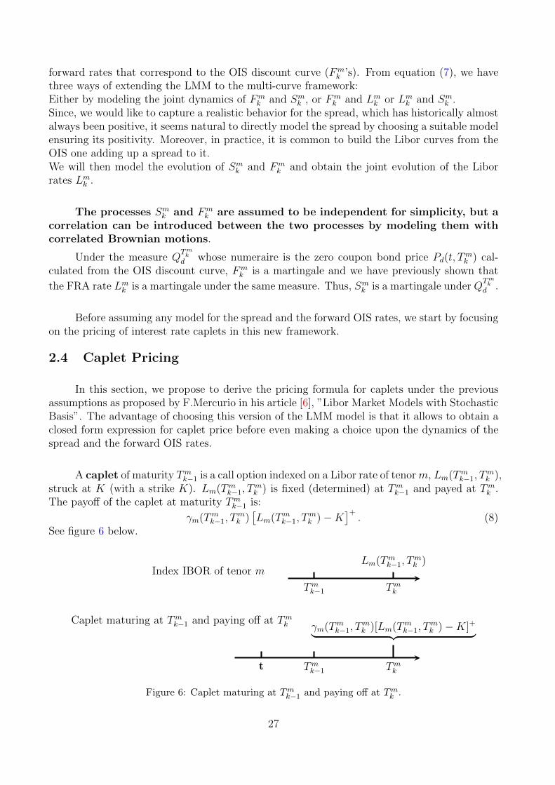
A caplet of maturity Tmk−1 is a call option indexed on a Libor rate of tenorm, Lm(Tmk−1, Tmk ),

struck at K (with a strike K). Lm(Tmk−1, Tmk ) is fixed (determined) at Tmk−1 and payed at Tmk .

The payoff of the caplet at maturity Tmk−1 is:

γm(Tmk−1, Tmk )[Lm(Tmk−1, T

mk )−K

]+. (8)

See figure 6 below.

Caplet maturing at Tmk−1 and paying off at Tmk

t Tmk−1 Tmk

γm(Tmk−1, Tmk )[Lm(Tmk−1, T

mk )−K]+︸ ︷︷ ︸

Index IBOR of tenor m

Tmk−1 Tmk

Lm(Tmk−1, Tmk )

Figure 6: Caplet maturing at Tmk−1 and paying off at Tmk .

27

Actually, the libor rate Lm(Tmk−1, Tmk ) is fixed two days prior to Tmk−1, but we have set

the fixing lag to 0 instead of 2 for simplicity. It is important to make the distinction herebetween the maturity date of the caplet, which corresponds to the date Tmk−1 where the Liboris fixed and the payment date of the caplet. In fact, the caplet pays off at its maturity dateTmk−1 but the payment is conventionally made at the end of the rate period Tmk .We denote by ΦC(t,K;Tmk−1, T

mk ) the price of the caplet at time t ≤ Tmk−1.

ΦC(t,K;Tmk−1, Tmk ) = γm(Tmk−1, T

mk )Pd(t, T

mk )EQ

Tmk

t [(Lm(Tmk−1, Tmk )−K)+]

= γm(Tmk−1, Tmk )Pd(t, T

mk )EQ

Tmk

t [(Lmk (Tmk−1)−K)+]

= γm(Tmk−1, Tk)Pd(t, Tmk )EQ

Tmk

t [(Smk (Tmk−1) + Fmk (Tmk−1)−K)+]

= γm(Tmk−1, Tmk )Pd(t, T

mk )EQ

Tmk

t

[(Smk (Tmk−1)− (K − Fm

k (Tmk−1)))+]

= γm(Tmk−1, Tmk )Pd(t, T

mk )EQ

Tmk

t

EQ

Tmk

[(Smk (Tmk−1)− (K − Fm

k (Tmk−1)))+ |Ft ∪ G

]where G is the sigma algebra generated by Fm

k (Tmk−1) and we have Ft ⊆ Ft ∪ G.

Since Fmk and Smk are independent, then:

EQTmk

[(Smk (Tmk−1)− (K − Fm

k (Tmk−1)))+ |Ft ∪ G

]= EQ

Tmk

t

[(Smk (Tmk−1)− (K − Fm

k (Tmk−1)))+],

so:

ΦC(t,K;Tmk−1, Tmk ) = γm(Tmk−1, T

mk )Pd(t, T

mk )

∫ +∞

−∞EQ

Tmk

t

[(Smk (Tmk−1)− (K − y)

)+]fFmk (Tmk−1)(y)dy,

where fFmk (Tmk−1) is the density function of Fmk (Tmk−1).

ΦC(t,K;Tmk−1, Tmk ) = γm(Tmk−1, T

mk )Pd(t, T

mk )

∫ K

−∞EQ

Tmk

t

[(Smk (Tmk−1)− (K − y)

)+]fFmk (Tmk−1)(y)dy

+

∫ +∞

K

EQTmk

t

[(Smk (Tmk−1)− (K − y)

)+]fFmk (Tmk−1)(y)dy

,

Here, we will make an assumption on the sign of Smk , which we suppose to be positive asit is the case historically. We will make sure to choose a positive stochastic process to representthe spread afterwards.

We have:∫ +∞

KEQ

Tmk

t

Smk (Tmk−1)− (K − y)︸ ︷︷ ︸

≤0

+ fFmk (Tm

k−1)(y)dy =

∫ +∞

KEQ

Tmk

t

[Smk (Tmk−1)− (K − y)

]fFmk

(Tmk−1

)(y)dy

=

∫ +∞

K[Smk (t)− (K − y)] fFm

k(Tmk−1

)(y)dy.

We set:ΦSC(t,K, Tmk−1, T

mk ) = γm(Tmk−1, T

mk )Pd(t, T

mk )EQ

Tmk

t [(Smk (Tmk−1)−K)+].

28

Hence,

ΦC(t,K;Tmk−1, Tmk ) =

∫ K

−∞ΦSc (t,K − y;Tmk−1, T

mk )fFm

k(Tmk−1

)(y)dy

+ γm(Tmk−1, Tmk )Pd(t, Tmk )

(Smk (t)−K)

∫ +∞

KfFmk

(Tmk−1

)(y)dy +

∫ +∞

KyfFm

k(Tmk−1

)(y)dy

=

∫ K

−∞ΦSc (t,K − y;Tmk−1, T

mk )fFm

k(Tmk−1

)(y)dy

+ γm(Tmk−1, Tmk )Pd(t, Tmk )

Smk (t)

∫ +∞

KfFmk

(Tmk−1

)(y)dy +

∫ +∞

K[y −K]fFm

k(Tmk−1

)(y)dy

.

We denote by ΦFC(t,K;Tmk−1, T

mk ) the price at time t of a caplet struck at K indexed to

the forward OIS rate Fm. So:

ΦFC(t,K;Tmk−1, T

mk ) = γm(Tmk−1, T

mk )Pd(t, T

mk )EQ

Tmk

t [(Fmk (Tmk−1)−K)+] =

∫ +∞

−∞[y −K]+ fFmk (Tmk−1)(y)dy

Deriving with respect to K leads to:∂

∂KΦFC(t,K;Tmk−1, T

mk ) = γm(Tmk−1, T

mk )Pd(t, Tmk )

∂

∂K

∫ +∞

K[y −K]fFm

k(Tmk−1

)(y)dy

= −γm(Tmk−1, T

mk )Pd(t, Tmk )

∫ +∞

KfFmk

(Tmk−1

)(y)dy

(9)

The demonstration of the last equality can be found in the annex.Finally, we obtain:

ΦC(t,K;Tmk−1, Tmk ) =

∫ K

−∞ΦSC(t,K − y;Tmk−1, T

mk )fFm

k(Tmk−1

)(y)dy − Smk (t)∂

∂KΦFC(t,K;Tmk−1, T

mk ) + ΦFC(t,K;Tmk−1, T

mk ) (10)

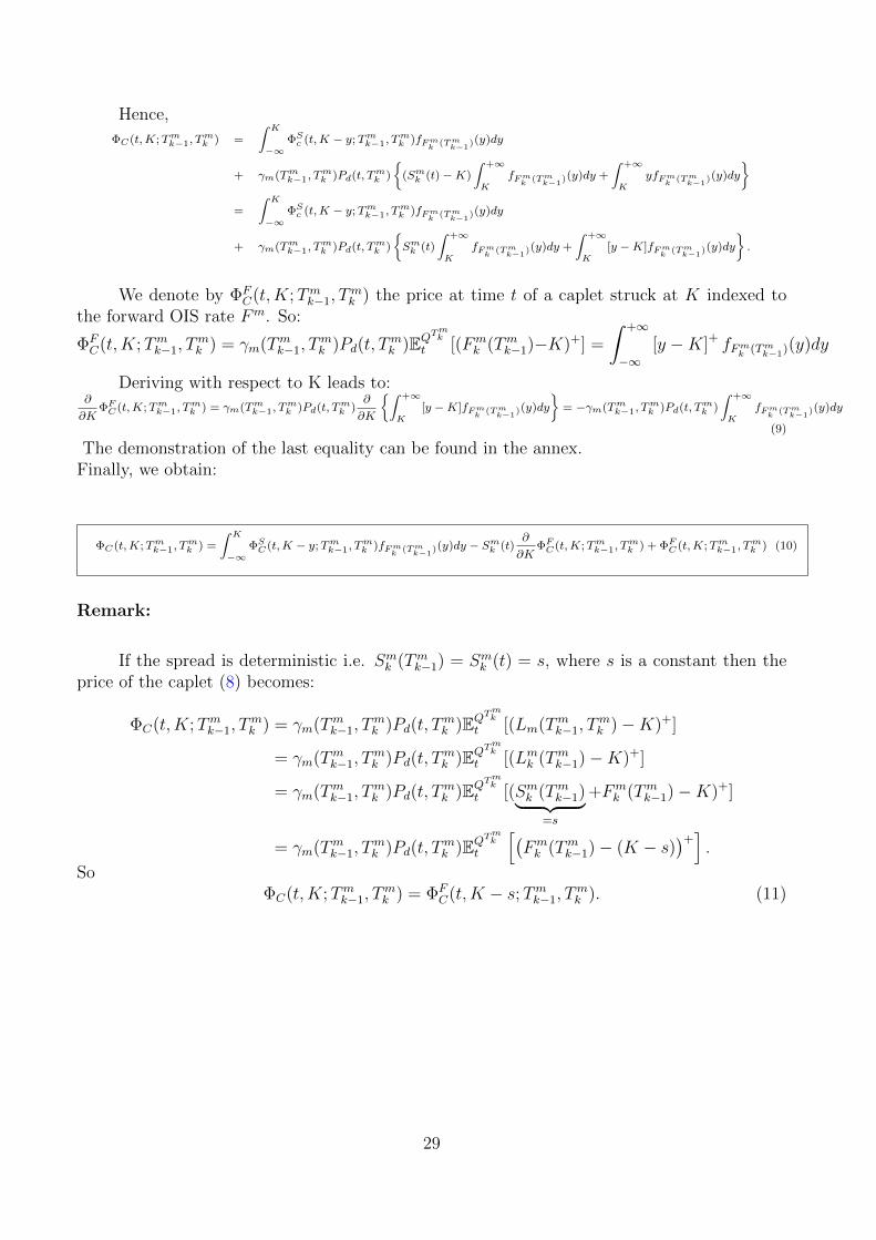
Remark:

If the spread is deterministic i.e. Smk (Tmk−1) = Smk (t) = s, where s is a constant then theprice of the caplet (8) becomes:

ΦC(t,K;Tmk−1, Tmk ) = γm(Tmk−1, T

mk )Pd(t, T

mk )EQ

Tmk

t [(Lm(Tmk−1, Tmk )−K)+]

= γm(Tmk−1, Tmk )Pd(t, T

mk )EQ

Tmk

t [(Lmk (Tmk−1)−K)+]

= γm(Tmk−1, Tmk )Pd(t, T

mk )EQ

Tmk

t [(Smk (Tmk−1)︸ ︷︷ ︸=s

+Fmk (Tmk−1)−K)+]

= γm(Tmk−1, Tmk )Pd(t, T

mk )EQ

Tmk

t

[(Fmk (Tmk−1)− (K − s)

)+].

SoΦC(t,K;Tmk−1, T

mk ) = ΦF

C(t,K − s;Tmk−1, Tmk ). (11)

29

3 Case Study

In this section, we propose to study a specific example of interest rate caplet pricing wheretwo specific dynamics are chosen for the evolution of the forward OIS rates and the spread.We propose to illustrate the example introduced by F.Mercurio [6], which assumes a shiftedlog-normal model for the forward OIS rates and SABR dynamics for the spread. It is importantto emphasize that this choice is not random as it ensures the positivity Sm and the fact theforward OIS rates Fm can be negative, which is possible with a shifted log-normal model.

Using these models will allow to explicite the caplet pricing formula (10) further.The resulting formula will then be implemented and used for the calibration of the overallmodel using market data.

Remark: The data used is provided by Bloomberg and corresponds to caps’ impliedvolatilities (for different strikes and maturities) and is provided in the annex. A bootstrappingprocedure allows to compute the underlying caplet implied volatilities and thus the correspond-ing prices, as it will be shown later.

A Monte Carlo method will then be presented and used for a comparison purpose, in orderto assess the accuracy of the formula, since the choice we will make on the spread dynamicscan lead us to obtain an approximation of the price ΦS

C only.Finally, a calibration will be conducted to test how well the chosen model can represent marketprices.

3.1 Dynamics for the Forwards OIS Rates and the Spread

As introduced above, the following dynamics will be considered for the Fmk (t) and

Smk (t) processes:

• OIS forward rates: Shifted Log-Normal

dFmk (t) = σmk

(Fmk (t) +

1

γmk

)dZm

k (t), (12)

where γmk is the year fraction corresponding to the period [Tmk−1, Tmk ], σmk > 0 depends on

the tenor and Zmk t≥0 is a standard Wiener process under the Q

Tmkd measure.

This SDE can easily be solved by defining a new process Gmk such that:

Gmk (t) = Fm

k (t) +1

γmk.

We then have:

dGmk (t) = dFm

k (t),

30

ordGm

k (t) = σmk Gmk (t)dZm

k (t).

The latter is the SDE of a log-normal process and can easily be solved using Ito’s lemma.As a matter of fact:

d(ln (Gmk (t))) =

dGmk (t)

Gmk (t)

− 1

2Gmk (t)

(dGmk (t))2︸ ︷︷ ︸

=(σmk )2Gmk (t)2dt

,

= −(σmk )2

2dt+ σmk dZ

mk (t).

We integrate the last equation between t and Tmk−1 and obtain:

Gmk (Tmk−1) = Gm

k (t)e

− (σmk )2

2(Tmk−1−t)+σ

mk (Zmk (Tmk−1)−Zmk (t))

,

So Gmk (Tmk−1) is a lognormmal process whose logarithm has a normal distribution with

mean ln (Gmk (t))− (σmk )2

2(Tmk−1 − t) and standard deviation σmk

√(Tmk−1 − t).

Finally,

Fmk (Tmk−1) +

1

γmk=

[Fmk (t) +

1

γmk

]e

− (σmk )2

2(Tmk−1−t)+σ

mk (Zmk (Tmk−1)−Zmk (t))

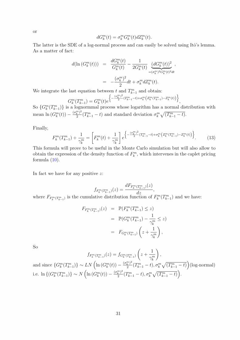
. (13)

This formula will prove to be useful in the Monte Carlo simulation but will also allow toobtain the expression of the density function of Fm

k , which intervenes in the caplet pricingformula (10).

In fact we have for any positive z:

fFmk (Tmk−1)(z) =dFFmk (Tmk−1)(z)

dz,

where FFmk (Tmk−1) is the cumulative distribution function of Fmk (Tmk−1) and we have:

FFmk (Tmk−1)(z) = P(Fmk (Tmk−1) ≤ z)

= P(Gmk (Tmk−1)− 1

γmk≤ z)

= FGmk (Tmk−1)

(z +

1

γmk

),

So

fFmk (Tmk−1)(z) = fGmk (Tmk−1)

(z +

1

γmk

),

and since Gmk (Tmk−1) ∼ LN

(ln (Gm

k (t))− (σmk )2

2(Tmk−1 − t), σmk

√(Tmk−1 − t)

)(log-normal)

i.e. ln (Gmk (Tmk−1) ∼ N

(ln (Gm

k (t))− (σmk )2

2(Tmk−1 − t), σmk

√(Tmk−1 − t)

).

31

We have:

fFmk (Tmk−1)(z) =1

σmk

(z + 1

γmk

)√2π(Tmk−1 − t)

exp

−[ln

(z+ 1

γmk

Fmk (t)+ 1γmk

)+ 1

2(σmk )2(Tmk−1 − t)

]2

2(σmk )2(Tmk−1 − t)

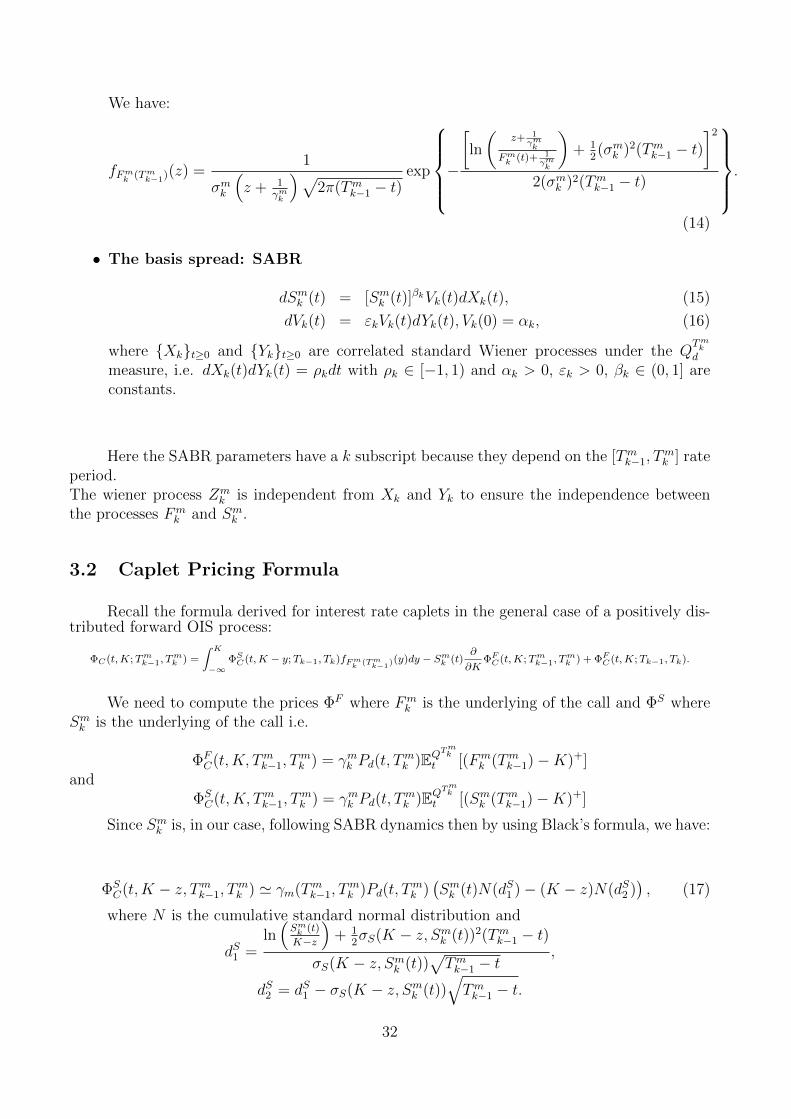
.(14)

• The basis spread: SABR

dSmk (t) = [Smk (t)]βkVk(t)dXk(t), (15)

dVk(t) = εkVk(t)dYk(t), Vk(0) = αk, (16)

where Xkt≥0 and Ykt≥0 are correlated standard Wiener processes under the QTmkd

measure, i.e. dXk(t)dYk(t) = ρkdt with ρk ∈ [−1, 1) and αk > 0, εk > 0, βk ∈ (0, 1] areconstants.

Here the SABR parameters have a k subscript because they depend on the [Tmk−1, Tmk ] rate

period.The wiener process Zm

k is independent from Xk and Yk to ensure the independence betweenthe processes Fm

k and Smk .

3.2 Caplet Pricing Formula

Recall the formula derived for interest rate caplets in the general case of a positively dis-tributed forward OIS process:

ΦC(t,K;Tmk−1, Tmk ) =

∫ K

−∞ΦSC(t,K − y;Tk−1, Tk)fFm

k(Tmk−1

)(y)dy − Smk (t)∂

∂KΦFC(t,K;Tmk−1, T

mk ) + ΦFC(t,K;Tk−1, Tk).

We need to compute the prices ΦF where Fmk is the underlying of the call and ΦS where

Smk is the underlying of the call i.e.

ΦFC(t,K, Tmk−1, T

mk ) = γmk Pd(t, T

mk )EQ

Tmk

t [(Fmk (Tmk−1)−K)+]

andΦSC(t,K, Tmk−1, T

mk ) = γmk Pd(t, T

mk )EQ

Tmk

t [(Smk (Tmk−1)−K)+]

Since Smk is, in our case, following SABR dynamics then by using Black’s formula, we have:

ΦSC(t,K − z, Tmk−1, T

mk ) ' γm(Tmk−1, T

mk )Pd(t, T

mk )(Smk (t)N(dS1 )− (K − z)N(dS2 )

), (17)

where N is the cumulative standard normal distribution and

dS1 =ln(Smk (t)

K−z

)+ 1

2σS(K − z, Smk (t))2(Tmk−1 − t)

σS(K − z, Smk (t))√Tmk−1 − t

,

dS2 = dS1 − σS(K − z, Smk (t))√Tmk−1 − t.

32

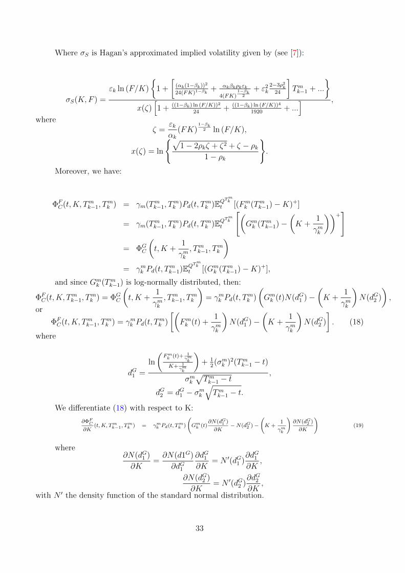
Where σS is Hagan’s approximated implied volatility given by (see [7]):

σS(K,F ) =

εk ln (F/K)

1 +

[(αk(1−βk))2

24(FK)1−βk+ αkβkρkεk

4(FK)1−βk

2

+ ε2k

2−3ρ2k24

]Tmk−1 + ...

x(ζ)

[1 + ((1−βk) ln (F/K))2

24+ ((1−βk) ln (F/K))4

1920+ ...

] ,

whereζ =

εkαk

(FK)1−βk

2 ln (F/K),

x(ζ) = ln

√1− 2ρkζ + ζ2 + ζ − ρk

1− ρk

.

Moreover, we have:

ΦFC(t,K, Tmk−1, T

mk ) = γm(Tmk−1, T

mk )Pd(t, T

mk )EQ

Tmk

t [(Fmk (Tmk−1)−K)+]

= γm(Tmk−1, Tmk )Pd(t, T

mk )EQ

Tmk

t

[(Gmk (Tmk−1)−

(K +

1

γmk

))+]

= ΦGC

(t,K +

1

γmk, Tmk−1, T

mk

)= γmk Pd(t, T

mk−1)EQ

Tmk

t [(Gmk (Tmk−1)−K)+],

and since Gmk (Tmk−1) is log-normally distributed, then:

ΦFC(t,K, Tmk−1, T

mk ) = ΦG

C

(t,K +

1

γmk, Tmk−1, T

mk

)= γmk Pd(t, T

mk )

(Gmk (t)N(dG1 )−

(K +

1

γmk

)N(dG2 )

),

or

ΦFC(t,K, Tmk−1, T

mk ) = γmk Pd(t, T

mk )

[(Fmk (t) +

1

γmk

)N(dG1 )−

(K +

1

γmk

)N(dG2 )

]. (18)

where

dG1 =

ln

(Fmk (t)+ 1

γmk

K+ 1γmk

)+ 1

2(σmk )2(Tmk−1 − t)

σmk√Tmk−1 − t

,

dG2 = dG1 − σmk√Tmk−1 − t.

We differentiate (18) with respect to K:

∂ΦFC∂K

(t,K, Tmk−1, Tmk ) = γmk Pd(t, Tmk )

(Gmk (t)

∂N(dG1 )

∂K−N(dG2 )−

(K +

1

γmk

)∂N(dG2 )

∂K

)(19)

where∂N(dG1 )

∂K=∂N(d1G)

∂dG1

∂dG1∂K

= N ′(dG1 )∂dG1∂K

,

∂N(dG2 )

∂K= N ′(dG2 )

∂dG2∂K

,

with N ′ the density function of the standard normal distribution.

33

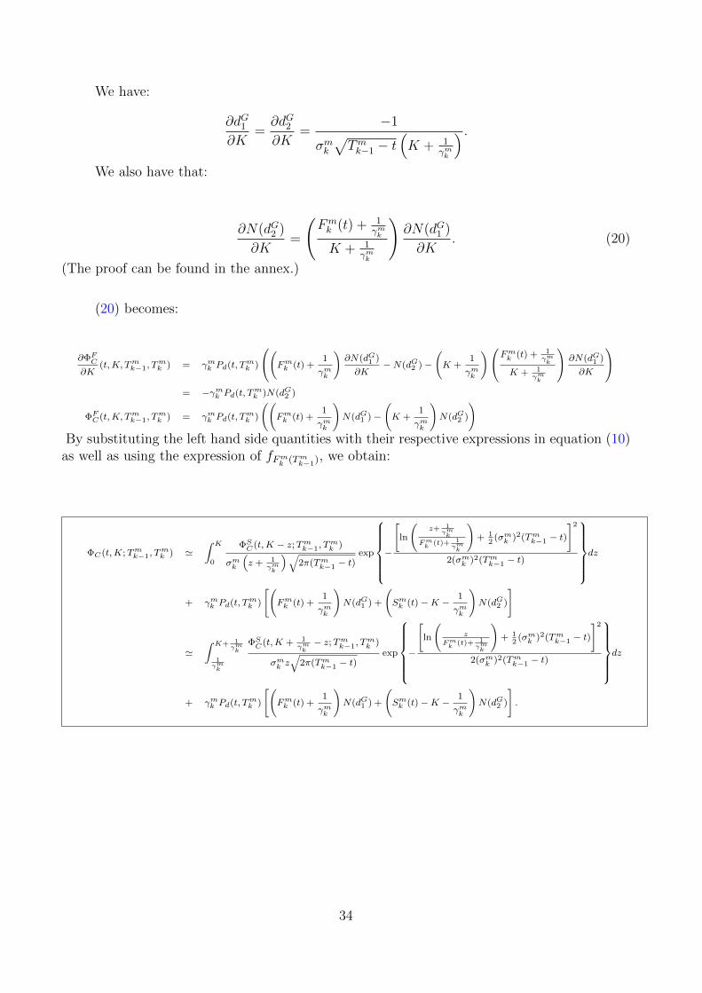
We have:

∂dG1∂K

=∂dG2∂K

=−1

σmk√Tmk−1 − t

(K + 1

γmk

) .We also have that:

∂N(dG2 )

∂K=

(Fmk (t) + 1

γmk

K + 1γmk

)∂N(dG1 )

∂K. (20)

(The proof can be found in the annex.)

(20) becomes:

∂ΦFC∂K

(t,K, Tmk−1, Tmk ) = γmk Pd(t, Tmk )

(Fmk (t) +1

γmk

)∂N(dG1 )

∂K−N(dG2 )−

(K +

1

γmk

)Fmk (t) + 1γmk

K + 1γmk

∂N(dG1 )

∂K

= −γmk Pd(t, Tmk )N(dG2 )

ΦFC(t,K, Tmk−1, Tmk ) = γmk Pd(t, Tmk )

((Fmk (t) +

1

γmk

)N(dG1 )−

(K +

1

γmk

)N(dG2 )

)By substituting the left hand side quantities with their respective expressions in equation (10)

as well as using the expression of fFmk (Tmk−1), we obtain:

ΦC(t,K;Tmk−1, Tmk ) '

∫ K

0

ΦSC(t,K − z;Tmk−1, Tmk )

σmk

(z + 1

γmk

)√2π(Tmk−1 − t)

exp

−

[ln

(z+ 1

γmk

Fmk

(t)+ 1γmk

)+ 1

2(σmk )2(Tmk−1 − t)

]22(σmk )2(Tmk−1 − t)

dz

+ γmk Pd(t, Tmk )

[(Fmk (t) +

1

γmk

)N(dG1 ) +

(Smk (t)−K −

1

γmk

)N(dG2 )

]

'∫ K+ 1

γmk

1γmk

ΦSC(t,K + 1γmk− z;Tmk−1, T

mk )

σmk z√

2π(Tmk−1 − t)exp

−

[ln

(z

Fmk

(t)+ 1γmk

)+ 1

2(σmk )2(Tmk−1 − t)

]22(σmk )2(Tmk−1 − t)

dz

+ γmk Pd(t, Tmk )

[(Fmk (t) +

1

γmk

)N(dG1 ) +

(Smk (t)−K −

1

γmk

)N(dG2 )

].

34

Remark:

If the spread is deterministic (recall (11)), then the price formula of the caplet becomes:

ΦC(t,K;Tmk−1, Tmk ) = γmk Pd(t, Tmk )

(Fmk (t) +

1

γmk

)N

ln

(Fmk (t)+ 1

γmk

K+s+ 1γmk

)+ 1

2(σmk )2(Tmk−1 − t)

σmk

√Tmk−1 − t

−(K + s+

1

γmk

)N

ln

(Fmk (t)+ 1

γmk

K+s+ 1γmk

)− 1

2(σmk )2(Tmk−1 − t)

σmk

√Tmk−1 − t

.

At this stage, we have derived the pricing formula for caplets under SABR dynamics forthe spread and shifted log-normal for the forward OIS rates, then we derived the formula incase of a deterministic spread but keeping the same shifted log-normal dynamics for the forwardOIS rates.The pricing formula when the spread is stochastic is an approximation because it involvesknowing the quantity ΦS

C (17), which is approximated by a Black price which uses the Haganapproximated implied volatility.To assess the accuracy of the pricing formula obtained, we propose to compare it to the outcomesof the Monte Carlo Method presented in the following section.

35

3.3 Monte Carlo Method

In this section, we propose to perform the caplet pricing using a Monte Carlo Methodwith an antithetic variance reduction method.We detail the procedure below:'

&

$

%

1. We choose a number M of simulations and at each simulation we repeat the followingsteps.

2. We use a simple forward Euler scheme to compute Smk (Tmk−1):

We first discretize the time interval [t, Tmk−1] into N small intervals of length ∆t =Tmk−1−tN

,thus defining a time grid t0 = t < t1 < ... < tN = Tmk−1; ∀i ∈ 1, 2, ..., n, ti − ti−1 = ∆t.The Forward Euler scheme allows to write:

Vk(ti) = Vk(ti−1) exp

−ε

2k

2∆t+ εk

√∆tY

,

Smk (ti) = Smk (ti−1) + [Smk (ti−1)]βkVk(ti−1)√

∆tX,where X and Y are realizations of two ρk-correlated wiener processes generated using aMersen-Twister algorithm for example. We simulate N times to obtain an approximationof

Smk (Tmk−1) 'n∑i=1

(Smk (ti−1))βkVk(ti−1)√

∆tX(ti−1).

3. We compute Fmk (Tmk−1) by simulating:

Fmk (Tmk−1) = − 1

γmk+

[Fmk (t) +

1

γmk

]e

− (σmk )2

2N∆t+σmk

√N∆tZ

,

where Z is a realization of a wiener process that is independent from X and Y .

4. Compute the payoff of the caplet:

γmk [Fmk (Tmk−1) + Smk (Tmk−1)−K]+.

5. For each simulation, we repeat steps 2, 3 and 4 by considering the opposite of all randomnumbers, as it must be done in an antithetic variance reduction method.

6. Compute the average payoff of the two methods (the one using the random numbersgenerated and the one using their opposites).

7. After running all M simulations, we compute the average of the M payoffs and discountthem using the right discount factor (Pd(t, T

mk )) obtained from the OIS discount curve

already created as of t (the pricing date).

This Monte Carlo method allowed to check the accuracy of the caplet pricing formula andas tables (4, 5 and 6) show, with around 10000 simulations and 10000 time steps, we obtainthe same values analytically and using the Monte Carlo method (a difference of order 10−8).

36

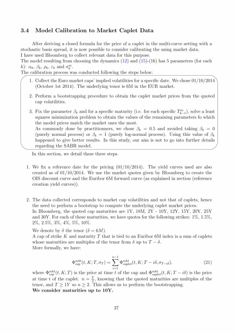
3.4 Model Calibration to Market Caplet Data

After deriving a closed formula for the price of a caplet in the multi-curve setting with astochastic basis spread, it is now possible to consider calibrating the using market data.I have used Bloomberg to collect relevant data for this purpose.The model resulting from choosing the dynamics (12) and (15)-(16) has 5 parameters (for eachk): αk, βk, ρk, εk and σmk .The calibration process was conducted following the steps below:'

&

$

%

1. Collect the Euro market caps’ implied volatilities for a specific date. We chose 01/10/2014(October 1st 2014). The underlying tenor is 6M in the EUR market.

2. Perform a bootstrapping procedure to obtain the caplet market prices from the quotedcap volatilities.

3. Fix the parameter βk and for a specific maturity (i.e. for each specific Tmk−1), solve a leastsquares minimization problem to obtain the values of the remaining parameters fo whichthe model prices match the market ones the most.As commonly done by practitionners, we chose βk = 0.5 and avoided taking βk = 0(purely normal process) or βk = 1 (purely log-normal process). Using this value of βkhappened to give better results. In this study, our aim is not to go into further detailsregarding the SABR model.

In this section, we detail these three steps.

1. We fix a reference date for the pricing (01/10/2014). The yield curves used are alsocreated as of 01/10/2014. We use the market quotes given by Bloomberg to create theOIS discount curve and the Euribor 6M forward curve (as explained in section (referencecreation yield curves)).

2. The data collected corresponds to market cap volatilities and not that of caplets, hencethe need to perform a bootstrap to compute the underlying caplet market prices.In Bloomberg, the quoted cap maturities are 1Y, 18M, 2Y - 10Y, 12Y, 15Y, 20Y, 25Yand 30Y. For each of these maturities, we have quotes for the following strikes: 1%, 1.5%,2%, 2.5%, 3%, 4%, 5%, 10%.

We denote by δ the tenor (δ = 6M).A cap of strike K and maturity T that is tied to an Euribor 6M index is a sum of capletswhose maturities are multiples of the tenor from δ up to T − δ.More formally, we have:

Φmktcap (t,K;T, σT ) =

n−1∑i=1

Φmktcaplet(t,K;T − iδ, σT−iδ), (21)

where Φmktcap (t,K;T ) is the price at time t of the cap and Φmkt

caplet(t,K;T − iδ) is the price

at time t of the caplet. n = Tδ, knowing that the quoted maturities are multiples of the

tenor, and T ≥ 1Y so n ≥ 2. This allows us to perform the bootstrapping.We consider maturities up to 10Y.

37

As a matter of fact, equation (21) rewrites into:

Φmktcaplet(t,K; δ, σ2δ) = Φmkt

cap (t,K; 2δ, σ2δ), (n = 2)

Φmktcaplet(t,K; 2δ, σ3δ) = Φmkt

cap (t,K; 3δ, σ3δ)− Φmktcap (t,K; 2δ, σ2δ), (n = 3)

Φmktcaplet(t,K; 3δ, σ4δ) = Φmkt

cap (t,K; 4δ, σ4δ)− Φmktcap (t,K; 3δ, σ3δ), (n = 4)

then for 3 ≤ i ≤ 10,Φmktcaplet(t,K; (2i− 1)δ, σ) + Φmktcaplet(t,K; 2(i− 1)δ, σ) = Φmktcap (t,K; 2iδ, σ2iδ)− Φmktcap (t,K; 2(i− 1)δ, σ2(i−1)δ)︸ ︷︷ ︸

θ

Here both caplets on the left hand side have the same volatility, which we are interestedin finding. For that, we define a function h of σ as the sum of two black formulaerepresenting the prices of the two caplets on the left hand side i.e.:For 3 ≤ i ≤ 10,

L1 = FRA(t, (2i− 1)δ, 2iδ), L2 = FRA(t, 2(i− 1)δ, (2i− 1)δ),

h(σ) = L1N

(ln (L1/K) + σ2/2

σ

)−KN

(ln (L1/K)− σ2/2

σ

)+ L2N

(ln (L2/K) + σ2/2

σ

)−KN

(ln (L2/K)− σ2/2

σ

)

The implied volatility of both caplets is the solution of the equation h(σ) = θ.

Once all the caplet volatilities are computed, we can use Black’s formula again for eachone of them to deduce their market prices.

3. Now that the relevant data is available, we can obtain the model parameters αk, ρk, εkand σδk that allow to match caplet market prices the most i.e.:

(αk, ρk, εk, σδk) = argminαk,ρk,εk,σ

δk

∑i

[ΦModelC (t,Ki, T )− Φmkt

C (t,Ki, T )]2

for a given maturity T ∈ δ, 2δ, ..., 20δ.

3.5 Numercial Results and Discussion

In this section, we present our results in terms of pricing and calibration.We have chosen to calibrate our model using EUR caplet data as of 01/10/2014. We performthe calibration for maturities 3Y, 4Y and 6Y.We will only consider data corresponding to strikes up to 3% because the rates asof 01/10/2010 are weak and the behaviour of the caplet prices for much higherstrikes cannot be controlled.Table 3 below presents the calibration results for these three maturities.

We notice that for the 6Y maturity, the calibration doesn’t seem to work properly. Fur-thermore, the correlation ρk varies drastically from a maturity to another, which can be ex-plained by the fact that the influence of this parameter is not high enough to affect the modelprices. We could as well fix it to zero (which is the convention insuring that no matter themeasure change i.e. no matter the forward measure, we have the same volatility dynamics) andcalibrate the other parameters. This would lead to the same results approximately. The ratherlow level of the spread (not exceeding 0.35% for its initial value) can explain the weak influenceof rhok as the contribution of the SABR dynamics in the caplet pricing formula is lower thanthat of the forward OIS dynamics, to which the prices are highly sensitive (parameter σmk ).

38

Caplet 3Y Caplet 4Y Caplet 6YExpiration date 02/10/2017 01/10/2018 01/10/2020

F 6Mk (t) 0.16873% 0.43822% 1.15707%

L6Mk (t) 0.50133% 0.78447% 1.46506%

S6Mk (t) 0.33260% 0.34625% 0.30799%αk 2.27% 2.05% 1.98%βk 0.5 0.5 0.5ρk 0.99 -0.99 0.99εk 40.00% 0.35% 1.00%

σ6Mk 0.1871% 0.236% 0.295%

Calibration error range [0.001382%; 0.16543%] [0.25999%; 2.12981%] [4.43970%; 50.67061%]

Table 3: Results of the calibration as of 01/10/2014.

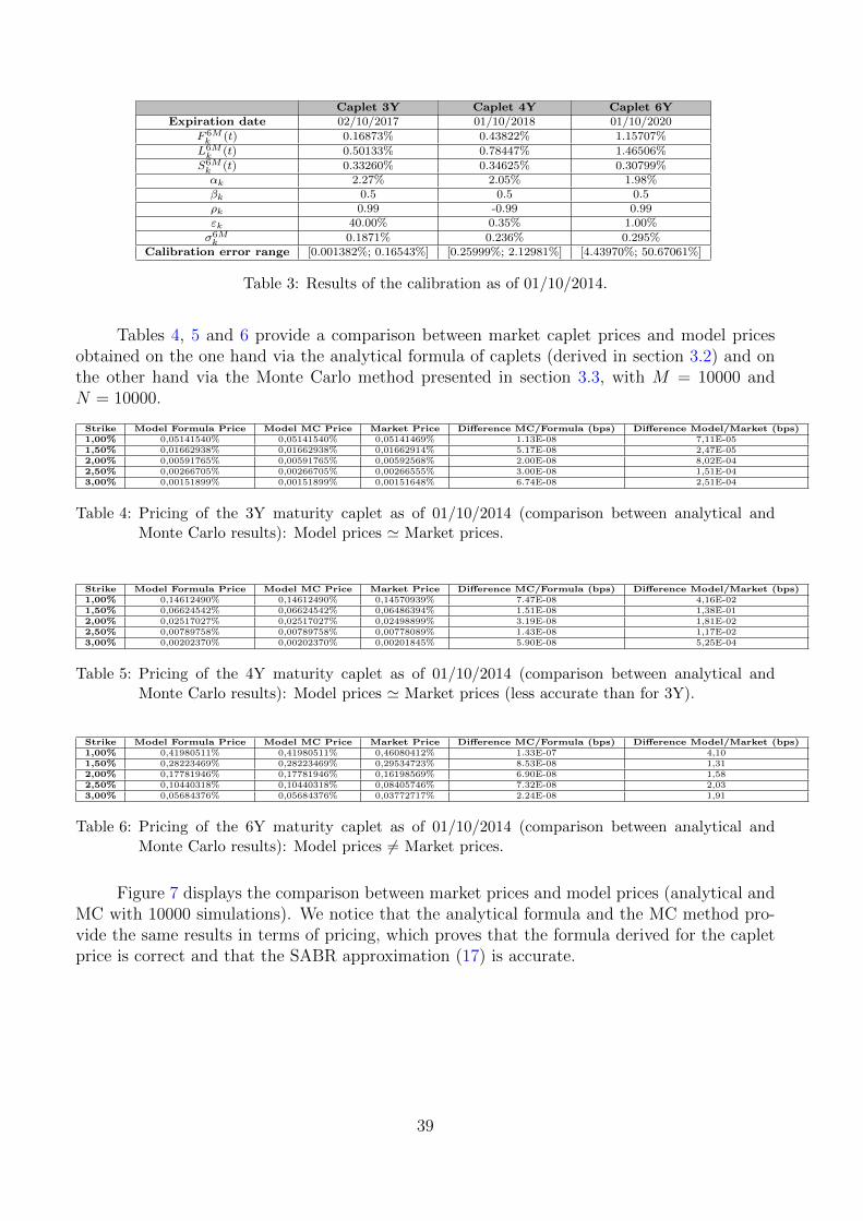
Tables 4, 5 and 6 provide a comparison between market caplet prices and model pricesobtained on the one hand via the analytical formula of caplets (derived in section 3.2) and onthe other hand via the Monte Carlo method presented in section 3.3, with M = 10000 andN = 10000.

Strike Model Formula Price Model MC Price Market Price Difference MC/Formula (bps) Difference Model/Market (bps)1,00% 0,05141540% 0,05141540% 0,05141469% 1.13E-08 7,11E-051,50% 0,01662938% 0,01662938% 0,01662914% 5.17E-08 2,47E-052,00% 0,00591765% 0,00591765% 0,00592568% 2.00E-08 8,02E-042,50% 0,00266705% 0,00266705% 0,00266555% 3.00E-08 1,51E-043,00% 0,00151899% 0,00151899% 0,00151648% 6.74E-08 2,51E-04

Table 4: Pricing of the 3Y maturity caplet as of 01/10/2014 (comparison between analytical andMonte Carlo results): Model prices ' Market prices.

Strike Model Formula Price Model MC Price Market Price Difference MC/Formula (bps) Difference Model/Market (bps)1,00% 0,14612490% 0,14612490% 0,14570939% 7.47E-08 4,16E-021,50% 0,06624542% 0,06624542% 0,06486394% 1.51E-08 1,38E-012,00% 0,02517027% 0,02517027% 0,02498899% 3.19E-08 1,81E-022,50% 0,00789758% 0,00789758% 0,00778089% 1.43E-08 1,17E-023,00% 0,00202370% 0,00202370% 0,00201845% 5.90E-08 5,25E-04

Table 5: Pricing of the 4Y maturity caplet as of 01/10/2014 (comparison between analytical andMonte Carlo results): Model prices ' Market prices (less accurate than for 3Y).

Strike Model Formula Price Model MC Price Market Price Difference MC/Formula (bps) Difference Model/Market (bps)1,00% 0,41980511% 0,41980511% 0,46080412% 1.33E-07 4,101,50% 0,28223469% 0,28223469% 0,29534723% 8.53E-08 1,312,00% 0,17781946% 0,17781946% 0,16198569% 6.90E-08 1,582,50% 0,10440318% 0,10440318% 0,08405746% 7.32E-08 2,033,00% 0,05684376% 0,05684376% 0,03772717% 2.24E-08 1,91

Table 6: Pricing of the 6Y maturity caplet as of 01/10/2014 (comparison between analytical andMonte Carlo results): Model prices 6= Market prices.

Figure 7 displays the comparison between market prices and model prices (analytical andMC with 10000 simulations). We notice that the analytical formula and the MC method pro-vide the same results in terms of pricing, which proves that the formula derived for the capletprice is correct and that the SABR approximation (17) is accurate.

39

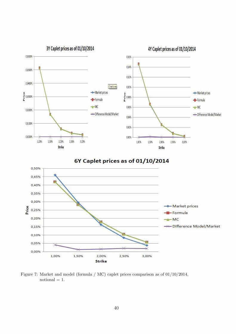
Figure 7: Market and model (formula / MC) caplet prices comparison as of 01/10/2014,notional = 1.

40

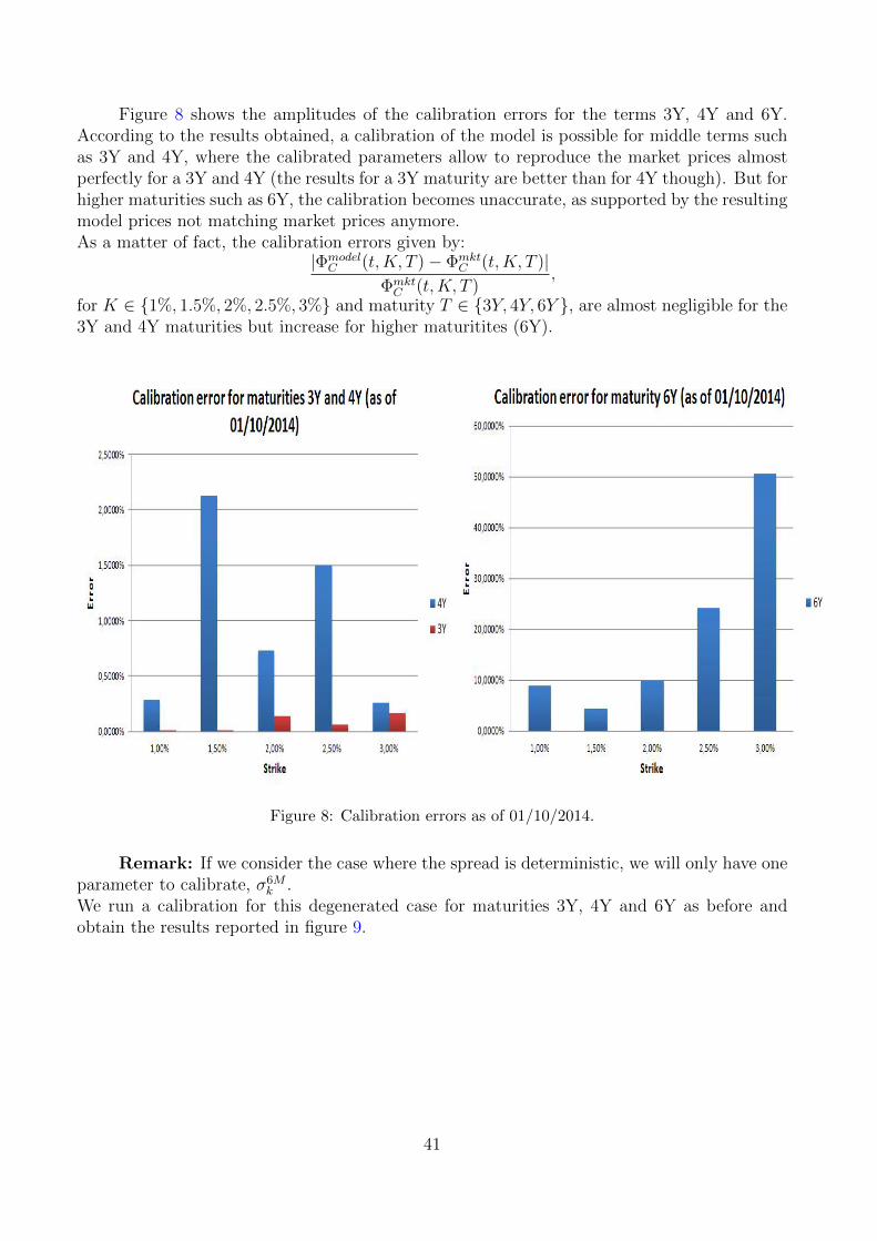
Figure 8 shows the amplitudes of the calibration errors for the terms 3Y, 4Y and 6Y.According to the results obtained, a calibration of the model is possible for middle terms suchas 3Y and 4Y, where the calibrated parameters allow to reproduce the market prices almostperfectly for a 3Y and 4Y (the results for a 3Y maturity are better than for 4Y though). But forhigher maturities such as 6Y, the calibration becomes unaccurate, as supported by the resultingmodel prices not matching market prices anymore.As a matter of fact, the calibration errors given by:

|ΦmodelC (t,K, T )− Φmkt

C (t,K, T )|ΦmktC (t,K, T )

,

for K ∈ 1%, 1.5%, 2%, 2.5%, 3% and maturity T ∈ 3Y, 4Y, 6Y , are almost negligible for the3Y and 4Y maturities but increase for higher maturitites (6Y).

Figure 8: Calibration errors as of 01/10/2014.

Remark: If we consider the case where the spread is deterministic, we will only have oneparameter to calibrate, σ6M

k .We run a calibration for this degenerated case for maturities 3Y, 4Y and 6Y as before andobtain the results reported in figure 9.

41

Figure 9: Market and model caplet prices comparison as of 01/10/2014 when using a model with adeterministic basis spread: σ6M

k = 0.335, σ6Mk = 0.379 and σ6M

k = 0.485 for 3Y, 4Y and 6Ymaturities respectively, notional = 1.

42

As we can observe from the figures, the calibration is not as accurate as when using astochastic spread for maturity 3Y and quickly becomes unaccurate for higher maturities asthe prices obtained via such a model cannot match the market prices for any choice of theparameter σ6M

k .From this comparison, we can understand the importance of including a stochastic feature andits impact on caplet prices (among other interest rate derivatives). Thus, models that use adeterministic spread don’t allow a good description of the market, which can be viewed throughour example, where the impact of the choice of the spread becomes obvious, now that the basisspread is no longer negligible as in the pre-crisis period.

The results emphasize the efficiency of the Libor Market Model when we calibrate usingcaplets of average maturities such as 3Y and 4Y. Meanwhile, the deterministic spread model isclearly not efficient even for average maturities.One difficulty here is that the level of the forward Euribor rates is relatively weak, so we haveless data to calibrate with as we cannot consider market data for strikes more than 3% forexample.The fact that for the date chosen (01/10/2014) the rates obtained are low, when performing acalibration using market caplets of strikes that are much higher than the FRA rates, the resultscan be disappointing. In our case, the lack of data for lower strikes forced us to consider strikesup to 3% (but not more), even if the level of forward rates as of 01/10/2014 is less than 1.5%.

We have tested our model on the same data set as used in Mercurio’s article, which cor-responded to February 8th, 2010, where the market was less stressed as the rates weren’t aslow as in our example. We managed to obtain good fits for even higher strikes (more than 3%),corroborating the results obtained in the article. We wanted, through this last test, emphasizethat the model calibration is very sensitive to the level of rates in the market.

To improve the calibration more, one can also add weights in order to give more impor-tance to one region of strikes where the FRA rates fall and less importance to the tails (verylow or very high strikes).

In our approach, we have been able to approach the market behaviour by using a classicalstochastic model for the basis spread, for average maturity caplets.Our model can be more adapted to other sets of data corresponding to a time when the marketis not stressed. In fact, If we take a look at the rates as of 01/10/2014 in the annex, we seethat some rates are negative, which corresponds to a stressed situation.

We insist on the fact that the LMM model is a tractable model, allowing to add morehypotheses and/or relax some others. It allows to derive closed formulae consequently. Thehardest part is to choose the most suitable dynamics for the quantitites we want to model asthis choice depends on the market changes. For example, in case of low rates, a log-normalmodel wouldn’t be a clever choice. In our example, the market situation as of 01/10/2014 (lowrates) didn’t allow for a very accurate fitting, which is the main dfficulty in this field.

Moreover, the choice of the instruments used in the calibration is very important as well.Unfortunately, there still doesn’t exist enough liquid instruments tied to the basis spread. Suchinstruments would have been more appropriate to use for the calibration.

43

4 Annex

4.1 Demonstrations

• We demonstrate the equality in equation (9):∂

∂K

∫ +∞

K

[y −K]fFmk (Tmk−1)(y)dy

= −

∫ +∞

K

fFmk (Tmk−1)(y)dy.

We have∂

∂K

∫ +∞

K[y −K]fFm

k(Tmk−1

)(y)dy

=

∂

∂K

∫ +∞

0[y −K]fFm

k(Tmk−1

)(y)1y≥Kdy

=

∫ +∞

0−1y≥KfFm

k(Tmk−1

)(y)dy +

∫ +∞

0(y −K)δK(y)fFm

k(Tmk−1

)(y)dy,

where δK is the Dirac function such that δK(y) = +∞ if y = K and δK(y) = 0 otherwise.So ∫ +∞

0

(y −K)δK(y)fFmk (Tmk−1)(y)dy = 0.

Which leads to the result.

• Equation (20):

∂N(dG2 )

∂K= N ′(dG2 )

∂dG2∂K

=1√2π

exp

−(dG2 )2

2

∂dG2∂K

=1√2π

exp

−

(dG1 )2 − 2dG1 σmk

√Tmk−1 − t+ (σmk )2(Tmk−1 − t)

2

∂dG2∂K

=1√2π

exp

−(dG1 )2

2

exp

−(σmk )2(Tmk−1 − t)

2+ dG1 σ

mk

√Tmk−1 − t

∂dG2∂K

= N ′(dG1 ) exp

ln

(Fmk (t) + 1

γmk

K + 1γmk

)∂dG1∂K

∂N(dG2 )

∂K=

(Fmk (t) + 1

γmk

K + 1γmk

)∂N(dG1 )

∂K.

4.2 Market Data

The market data used for yield curve construction/bootstrapping are the EUR data as of01/10/2014 is given in the tables below:

44

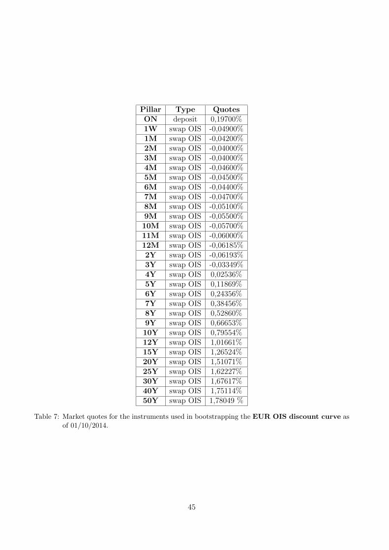
Pillar Type QuotesON deposit 0,19700%1W swap OIS -0,04900%1M swap OIS -0,04200%2M swap OIS -0,04000%3M swap OIS -0,04000%4M swap OIS -0,04600%5M swap OIS -0,04500%6M swap OIS -0,04400%7M swap OIS -0,04700%8M swap OIS -0,05100%9M swap OIS -0,05500%10M swap OIS -0,05700%11M swap OIS -0,06000%12M swap OIS -0,06185%2Y swap OIS -0,06193%3Y swap OIS -0,03349%4Y swap OIS 0,02536%5Y swap OIS 0,11869%6Y swap OIS 0,24356%7Y swap OIS 0,38456%8Y swap OIS 0,52860%9Y swap OIS 0,66653%10Y swap OIS 0,79554%12Y swap OIS 1,01661%15Y swap OIS 1,26524%20Y swap OIS 1,51071%25Y swap OIS 1,62227%30Y swap OIS 1,67617%40Y swap OIS 1,75114%50Y swap OIS 1,78049 %

Table 7: Market quotes for the instruments used in bootstrapping the EUR OIS discount curve asof 01/10/2014.

45

Pillar Type QuotesON deposit 0,18100%1W deposit 0,18470%1M deposit 0,19458%2M deposit 0,20692%3M deposit 0,19745%4M deposit 0,18905%5M deposit 0,18706%6M deposit 0,18100%7M deposit 0,17889%8M deposit 0,17782%9M deposit 0,17577%10M deposit 0,17241%11M deposit 0,17062%12M swap 6M 0,16996%2Y swap 6M 0,18629%3Y swap 6M 0,23700%4Y swap 6M 0,31500%5Y swap 6M 0,42200%6Y swap 6M 0,55000%7Y swap 6M 0,692%8Y swap 6M 0,835 %9Y swap 6M 0,97100 %10Y swap 6M 1,09500 %12Y swap 6M 1,30500 %15Y swap 6M 1,53100 %20Y swap 6M 1,74300 %25Y swap 6M 1,83200 %30Y swap 6M 1,86800 %40Y swap 6M 1,91600 %50Y swap 6M 1,92500 %

Table 8: Market quotes for the instruments used in bootstrapping the EURIBOR 6M forwardcurve as of 01/10/2014.

The following table provides the market cap implied volatility data as of 01/10/2014 usedin the calibration process, precisely in the bootstrapping of caplet market prices.

46

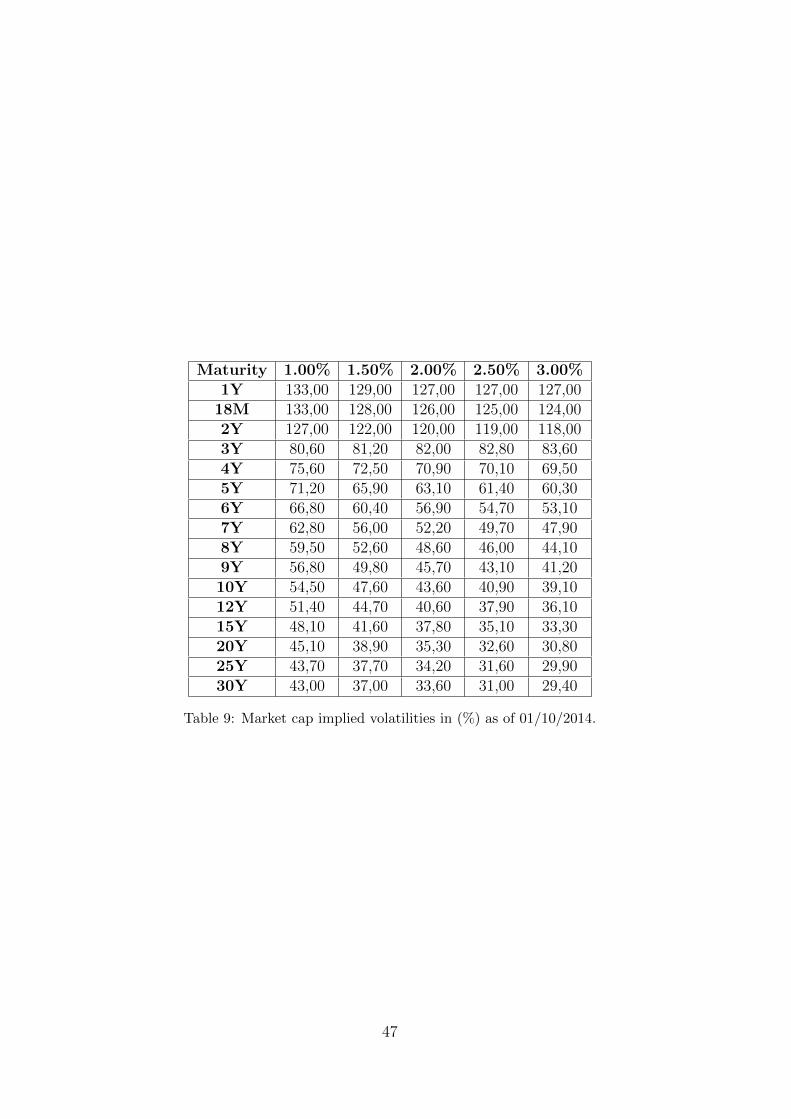
Maturity 1.00% 1.50% 2.00% 2.50% 3.00%1Y 133,00 129,00 127,00 127,00 127,00

18M 133,00 128,00 126,00 125,00 124,002Y 127,00 122,00 120,00 119,00 118,003Y 80,60 81,20 82,00 82,80 83,604Y 75,60 72,50 70,90 70,10 69,505Y 71,20 65,90 63,10 61,40 60,306Y 66,80 60,40 56,90 54,70 53,107Y 62,80 56,00 52,20 49,70 47,908Y 59,50 52,60 48,60 46,00 44,109Y 56,80 49,80 45,70 43,10 41,2010Y 54,50 47,60 43,60 40,90 39,1012Y 51,40 44,70 40,60 37,90 36,1015Y 48,10 41,60 37,80 35,10 33,3020Y 45,10 38,90 35,30 32,60 30,8025Y 43,70 37,70 34,20 31,60 29,9030Y 43,00 37,00 33,60 31,00 29,40

Table 9: Market cap implied volatilities in (%) as of 01/10/2014.

47

References

[1] Marco Bianchetti; Interest Rates After The Credit Crunch: Multiple-Curve Vanilla Deriva-tives and SABR, 2012.

[2] Ferdinando M. Ametrano, Marco Bianchetti; Everything You Always Wanted to Know AboutMultiple Interest Rate Curve Bootstrapping But Were Afraid To Ask, Version: 2 April 2013.

[3] Fabio Mercurio, QFR, Bloomberg; Interest Rates and The Credit Crunch: New Formulasand Market Models, 2009.

[4] M. Fujii, Y. Shimada, A. Takahashi; A Market Model of Interest Rates with Dynamic BasisSpreads in the presence of Collateral and Multiple Currencies, 2009.

[5] Marco Bianchetti; Two Curves, One Price: Pricing & Hedging Interest Rate Derivatives,Decoupling Forwarding and Discounting Yield Curves, 2012.

[6] Fabio Mercurio; LIBOR Market Models with Stochastic Basis.

[7] Hagan, P and A.Lesniewski (2008); LIBOR market model with SABR style stochastic volatil-ity. Online at:

http://www.lesniewski.us/papers/working/SABRLMM.pdf

[8] Z. El Menouni (2014); Yield Curve Bootstrapping/ Pricing of Plain Vanilla IRS and BasisSwaps in SAP (confidential)

48

TRITA -MAT-E 2015:09

ISRN -KTH/MAT/E-15/09--SE

www.kth.se