Pricing Inflation Derivatives

Pricing Inflation Derivatives

A survey of short rate- and market models

D A M R T E W O L D E B E R H A N

Master of Science Thesis Stockholm, Sweden 2012

Pricing Inflation Derivatives

A survey of short rate- and market models

D A M R T E W O L D E B E R H A N

Degree Project in Mathematical Statistics (30 ECTS credits) Degree Programme in Computer Science and Engineering 270 credits

Royal Institute of Technology year 2012 Supervisor at KTH was Boualem Djehiche

Examiner was Boualem Djehiche TRITA-MAT-E 2012:13 ISRN-KTH/MAT/E--12/13--SE Royal Institute of Technology School of Engineering Sciences KTH SCI SE-100 44 Stockholm, Sweden URL: www.kth.se/sci

AbstractThis thesis presents an overview of strategies for pricing inflation deriva-tives. The paper is structured as follows. Firstly, the basic definitionsand concepts such as nominal-, real- and inflation rates are introduced.We introduce the benchmark contracts of the inflation derivatives mar-ket, and using standard results from no-arbitrage pricing theory, derivepricing formulas for linear contracts on inflation. In addition, the riskprofile of inflation contracts is illustrated and we highlight how it’s cap-tured in the models to be studied studied in the paper.

We then move on to the main objective of the thesis and presentthree approaches for pricing inflation derivatives, where we focus inparticular on two popular models. The first one, is a so called HJMapproach, that models the nominal and real forward curves and relatesthe two by making an analogy to domestic and foreign fx rates. Bythe choice of volatility functions in the HJM framework, we producenominal and real term structures similar to the popular interest-ratederivatives model of Hull-White. This approach was first suggested byJarrow and Yildirim[1] and it’s main attractiveness lies in that it resultsin analytic pricing formulas for both linear and non-linear benchmarkinflation derivatives.

The second approach, is a so called market model, independentlyproposed by Mercurio[2] and Belgrade, Benhamou, and Koehler[4]. Justlike the - famous - Libor Market Model, the modeled quantities are ob-servable market entities, namely, the respective forward inflation indices.It is shown how this model as well - by the use of certain approxima-tions - can produce analytic formulas for both linear and non-linearbenchmark inflation derivatives.

The advantages and shortcomings of the respective models are evelu-ated. In particular, we focus on how well the models calibrate to marketdata. To this end, model parameters are calibrated to market prices ofyear-on-year inflation floors; and it is evaluated how well market pricescan be recovered by theoretical pricing with the calibrated model param-eters. The thesis is concluded with suggestions for possible extensionsand improvements.

Contents

1 Introduction 11.1 Inflation Basics . . . . . . . . . . . . . . . . . . . . . . . . . . . . . . 1

1.1.1 Inflation, nominal value and real value . . . . . . . . . . . . . 11.1.2 Inflation Index . . . . . . . . . . . . . . . . . . . . . . . . . . 1

1.2 Overview of Inflation-Linked Instruments . . . . . . . . . . . . . . . 21.2.1 Inflation-Linked Bond . . . . . . . . . . . . . . . . . . . . . . 21.2.2 Zero Coupon Inflation Swap . . . . . . . . . . . . . . . . . . . 31.2.3 Year On Year Inflation Swap . . . . . . . . . . . . . . . . . . 61.2.4 Inflation Linked Cap/Floor . . . . . . . . . . . . . . . . . . . 7

1.3 Inflation and interest rate risk . . . . . . . . . . . . . . . . . . . . . . 81.3.1 Breakeven inflation vs expected inflation . . . . . . . . . . . . 81.3.2 Inflation risk . . . . . . . . . . . . . . . . . . . . . . . . . . . 10

2 The HJM framework of Jarrow and Yildirim 112.1 Definitions . . . . . . . . . . . . . . . . . . . . . . . . . . . . . . . . . 112.2 Model specification . . . . . . . . . . . . . . . . . . . . . . . . . . . . 112.3 Zero Coupon Bond term structure . . . . . . . . . . . . . . . . . . . 14

2.3.1 General form . . . . . . . . . . . . . . . . . . . . . . . . . . . 142.3.2 Jarrow Yildirim drift conditions . . . . . . . . . . . . . . . . 14

2.4 Hull-White specification . . . . . . . . . . . . . . . . . . . . . . . . . 162.4.1 Nominal term structure . . . . . . . . . . . . . . . . . . . . . 162.4.2 Real term structure . . . . . . . . . . . . . . . . . . . . . . . 18

2.5 Year-On-Year Inflation Swap . . . . . . . . . . . . . . . . . . . . . . 182.6 Inflation Linked Cap/Floor . . . . . . . . . . . . . . . . . . . . . . . 20

3 Market Model I - A Libor Market Model for nominal and realforward rates 233.1 Year-On-Year Inflation Swap . . . . . . . . . . . . . . . . . . . . . . 233.2 Inflation Linked Cap/Floor . . . . . . . . . . . . . . . . . . . . . . . 26

4 Market Model II - Modeling the forward inflation indices 294.1 Year-On-Year Inflation Swap . . . . . . . . . . . . . . . . . . . . . . 294.2 Inflation Linked Cap/Floor . . . . . . . . . . . . . . . . . . . . . . . 31

5 Calibration 335.1 Nominal- and Real Curves . . . . . . . . . . . . . . . . . . . . . . . . 335.2 Simplified Jarrow-Yildirim Model . . . . . . . . . . . . . . . . . . . . 355.3 Jarrow Yildirim Model . . . . . . . . . . . . . . . . . . . . . . . . . . 38

5.3.1 Calibrating nominal volatility parameters to ATM Cap volatil-ities . . . . . . . . . . . . . . . . . . . . . . . . . . . . . . . . 38

5.3.2 Fitting parameters to Year-On-Year Inflation Cap quotes . . 395.4 Market Model II . . . . . . . . . . . . . . . . . . . . . . . . . . . . . 43

5.4.1 Nominal volatility parameters . . . . . . . . . . . . . . . . . . 435.4.2 Fitting parameters to Year-On-Year Inflation Cap quotes . . 43

6 Conclusions and extensions 456.1 Conclusions . . . . . . . . . . . . . . . . . . . . . . . . . . . . . . . . 456.2 Extensions . . . . . . . . . . . . . . . . . . . . . . . . . . . . . . . . . 46

A Appendix 47A.1 Change of numeraire . . . . . . . . . . . . . . . . . . . . . . . . . . . 47

References 49

Chapter 1

Introduction

1.1 Inflation Basics

1.1.1 Inflation, nominal value and real value

An investor is concerned with the real return of an investment. That is, interestedin the quantity of goods and services that can be bought with the nominal return.For instance, a 2% nominal return and no increase in prices of goods and services ispreferred to a 10% nominal return and a 10% increase in prices of goods and services.Put differently, the real value of the nominal return is subjected to inflation risk,where inflation is defined as the relative increase of prices of goods and services.

Inflation derivatives are designed to transfer the inflation risk between two par-ties. The instruments are typically linked to the value of a basket, reflecting pricesof goods and services used by an average consumer. The value of the basket iscalled an Inflation Index. Well known examples are the HICPxT(EUR), RPI(UK),CPI(FR) and CPI(US) indices.

The index is typically constructed such that the start value is normalized to 100at a chosen base date. At regular intervals the price of the basket is updated andthe value of the index ix recalculated. The real return of an investment can thenbe defined as the excess nominal return over the relative increase of the inflationindex.

1.1.2 Inflation Index

Ideally, we would like to have access to index values on a daily basis, so that anycash flow can be linked to the corresponding inflation level at cash flow pay date.For practical reasons this is not possible. It takes time to compute and publish theindex value. Due to this, inflation linked cash flows are subjected to a so-calledindexation lag. That is, the cash flow is linked to an index value referencing ahistorical inflation level. The lag differs for different markets. For example thelag for the HICPxt daily reference number is three months. As a consequence,an investor who wishes to buy protection against inflation, has inflation exposure

1

CHAPTER 1. INTRODUCTION

during the last three months before maturity of the inflation protection instrument.That is, the last three months it is effectively a nominal instrument.

1.2 Overview of Inflation-Linked Instruments

1.2.1 Inflation-Linked BondDefinition

An inflation-linked zero coupon bond is a bond that pays out a single cash flow atmaturity TM , consisting of the increase in the reference index between issue dateand maturity. We set the reference index to I0 at issue date (t = 0) and a contractsize of N units. The (nominal) value is denoted as ZCILB(t, TM , I0, N). Thenominal payment consists of

N

I0I(TM ) (1.2.1)

nominal units at maturity. The corresponding real amount is obtained by normal-izing with the time TM index value. That is, we receive

N

I0(1.2.2)

real units at maturity. It’s thus clear that an inflation-linked zero coupon bond paysout a known real amount, but an unknown nominal amount, which is fixed when wereach the maturity date.

Pricing

Let Pr(t, TM ) denote the time t real value of 1 unit paid at time TM . Then

N

I0Pr(t, TM )

expresses the time t real value of receiving N/I0 units at TM , which is the definitionof the payout of the ZCILB. And since the time t real value of the ZCILB is obtainedby normalizing the nominal value with the inflation index we have

ZCILB(t, TM , I0, N)I(t)

= NPr(t, TM )I0

(1.2.3)

Defining the bonds unit value as PIL(t, TM ) := ZCILB(t, TM , 1, 1) we get

PIL(t, TM ) = I(t)Pr(t, TM ) (1.2.4)

Thus the price of the bond is dependent on inflation index levels and the realdiscount rate.

In practice, as in the nominal bond market, the inflation bonds issued are typ-ically coupon bearing. The coupon inflation bond can be replicated as the sum of

2

1.2. OVERVIEW OF INFLATION-LINKED INSTRUMENTS

a series of zero coupon inflation bonds. With C denoting the annual coupon rate, TM the maturity date, N the contract size , I0 the index value at issue date andassuming annual coupon frequency, the nominal time t value of a coupon bearinginflation-linked bond is given as

ILB(t, TM , I0, N) = N

I0

[C

M∑i=1

PIL(t, Ti) + PIL(t, TM )]

= I(t)I0

N

[C

M∑i=1

Pr(t, Ti) + Pr(t, TM )] (1.2.5)

1.2.2 Zero Coupon Inflation SwapDefinition

A zero coupon inflation swap is a contract where the inflation seller pays the inflationindex rate between today and TM , and the inflation buyer pays a fixed rate. Thepayout on the inflation leg is given by

N

[I(TM )I0

− 1]

(1.2.6)

Thus, the inflation leg pays the net increase in reference index. The payout on thefixed side of the swap is agreed upon at inception and is given as

N[(1 + b(0, TM ))TM − 1

](1.2.7)

where b is the so called breakeven inflation rate. In the market, b is quoted suchthat the induced TM maturity zero coupon inflation swap has zero value today. It’sanalogous to the par rates quoted in the nominal swap market.

From the payout of the inflation leg, it’s clear that it can be valued in terms of aninflation linked and a nominal zero coupon bond. However we shall proceed with abit more formal derivation as it will be useful when proceeding to more complicatedinstrument types.

Foreign markets and numeraire change

Consider a foreign market where an asset with price Xf is traded. Denote by Qf theassociated (foreign) martingale measure. Assume that the foreign money marketaccount evolves according to the process Bf . Analogously, consider a domesticmarket with domestic money market account evolving according to the process Bd.Let the exchange rate between the two currencies be modeled by the process H, sothat 1 unit of the foreign currency is worth H(t) units of domestic currency at timet. Let F = Ft : 0 ≤ t ≤ TM be the filtration generated by the above processes.

If we think of Xf as a derivative that pays out Xf (TM ) at time TM , by standardno-arbitrage pricing theory, the arbitrage free price in the foreign market at time t

3


is

Vf (t) = Bf (t)EQf

[Xf (TM )Bf (TM )

∣∣∣∣∣Ft

](1.2.8)

Or expressed as a price in the domestic currency

Vd(t) = H(t)Bf (t)EQf

[Xf (TM )Bf (TM )

∣∣∣∣∣Ft

](1.2.9)

Note, that for a domestic investor who buys the (foreign) asset Xf , the payout attime TM is Xf (TM )H(TM ). Now consider a domestic derivative which at time TM

pays out Xf (TM )H(TM ). To avoid arbitrage, the price of this instrument must beequal to price of the foreign asset multiplied with the spot exchange rate. So we getthe relation

H(t)Bf (t)EQf

[Xf (TM )Bf (TM )

∣∣∣∣∣Ft

]= Bd(t)EQd

[H(TM )Xf (TM )

Bd(TM )

∣∣∣∣Ft

](1.2.10)

Pricing

Using well known results from standard no-arbitrage pricing theory, with obviouschoice of notations, we get the time t value of the inflation leg as

ZCILS(t, TM , I0, N) = NEQn

[e−∫ TM

trn(u)du

(I(TM )I0

− 1)∣∣∣∣Ft

](1.2.11)

We draw a foreign currency analogy, namely that real prices correspond to foreignprices and nominal prices correspond to domestic prices. The inflation index valuethen corresponds to the domestic currency/foreign currency spot exchange rate.Applying the result from (1.2.10) we then obtain

I(t)Pr(t, TM ) = I(t)EQr

[e−∫ TM

trr(u)du

∣∣∣∣Ft

]= EQn

[I(TM ) e−

∫ TMt

rn(u)du∣∣∣∣Ft

](1.2.12)

Putting this into (1.2.11) yields

ZCILS(t, TM , I0, N) = N

[I(t)I(0)

Pr(t, TM ) − Pn(t, TM )]

(1.2.13)

which at time t = 0 simplifies to

ZCILS(0, TM , I0, N) = N [Pr(0, TM ) − Pn(0, TM )] (1.2.14)

Important to note is that these prices do not depend on any assumptions of thedynamics of the interest rate market, but rather follow from the absence of arbitrage.This is an imortant result, as it will enable us to calibrate the real rate discount

4


0 5 10 15 20 25 30

0.8

1

1.2

1.4

1.6

1.8

2

2.2

2.4

2.6

Maturity(years)

Rat

e(%

)

Swap Rates (EUR)Break−Even Inflation Rates (EUR)

Figure 1.1: Quotes for European nominal- and Zero-Coupon Inflation Swaps, 13jul-2012

curve from prices of index linked zero-coupon swaps by, for each swap, solving thepar value relation. That is , when entering the contract, the value of the pay legshould equal the receive leg.

NPn(0, TM )[(1 + b(0, TM ))TM − 1] = N [Pr(0, TM ) − Pn(0, TM )] (1.2.15)

which gives us the real discount rate as

Pr(0, TM ) = Pn(0, TM )(1 + b(0, TM ))TM (1.2.16)

where b is the (market quoted) break-even inflation rate and Pn(0, TM ) can berecovered from bootstrapping the nominal discount curve.

Figure 1.1 shows quotes for break-even inflation rates and nominal swap rates.The maturities up to the 10-year mark reveal something interesting. The nominalswap quote is the fixed rate one would demand in exchange for paying floatingcash flows of EURIBOR until maturity. Whereas the break-even inflation quote isthe fixed rate one would would demand in exchange for paying realized inflation

5


rate until maturity. The gap between the two, i.e. that the swap quote is lower,indicates that expected inflation is higher than expected EURIBOR. This in turnimplies negative real rates. We discuss break-even inflation visavis expected inflationin more detail in section (1.3.1).

1.2.3 Year On Year Inflation Swap

Definition

The inflation leg on a Year On Year Inflation Swap pays out a series of net increasesin index reference

NM∑

i=1

[I(Ti)I(Ti−1)

− 1]ψi (1.2.17)

where ψi is the time in years on the interval [Ti−1, Ti];T0 := 0 according to thecontracts day-count convention.

The fixed leg pays a series of fixed coupons

NM∑

i=1ψiC (1.2.18)

Just as for Zero Coupon Inflation swaps , Year On Year Inflation Swaps are quotedin the market in terms of their fixed coupon. However out of the two, the formeris more liquid , and is considered to be the primary benchmark instrument in theinflation derivatives market.

Pricing

We can view (1.2.17) as a series of forward starting Zero Coupon Swap Inflationlegs. Then the price of each leg is

YYILS(t, Ti−1, Ti, ψi, N) = NψiEQn

[e−∫ Ti

trn(u)du

(I(Ti)I(Ti−1)

− 1)∣∣∣∣Ft

](1.2.19)

If t > Ti−1 so that I(Ti−1) is known then it reduces to the pricing of a regular ZeroCoupon Swap Inflation leg. If t < Ti−1 then we use repeated expectation to get

YYILS(t, Ti−1, Ti, ψi, N)

= NψiEQn

[EQn

[e−∫ Ti

trn(u)du

(I(Ti)I(Ti−1)

− 1)∣∣∣∣FT −1

]∣∣∣∣Ft

]= NψiE

Qn

[e−∫ Ti−1

trn(u)duEQn

[e

−∫ Ti

T −1 rn(u)du(I(Ti)I(Ti−1)

− 1)∣∣∣∣FT −1

]∣∣∣∣Ft

](1.2.20)

6


The inner expection is recognized as ZCILS(Ti−1, Ti, I(Ti−1), 1) so that we finallyobtain

YYIIS(t, Ti−1, Ti, ψi, N) = NψiEQn

[e−∫ Ti−1

trn(u)du [Pr(Ti−1, Ti) − Pn(Ti−1, Ti)]

∣∣∣∣Ft

]= NψiE

Qn

[e−∫ Ti−1

trn(u)duPr(Ti−1, Ti)

∣∣∣∣Ft

]−NψiPn(t, Ti)

(1.2.21)

The last expectation can be interpreted as the nominal price of a derivative payingout at time Ti−1 (in nominal units) the Ti maturity real zero coupon bond price. Ifreal rates were deterministic then we would get

EQn

[e−∫ Ti−1

trn(u)duPr(Ti−1, Ti)

∣∣∣∣Ft

]= Pn(t, Ti−1)Pr(Ti−1, Ti)

= Pn(t, Ti−1) Pr(t, Ti)Pr(t, Ti−1)

which is simply the nominal present value of the Ti−1 forward price of the Ti ma-turity real bond. In practice however it’s not realistic to assume that real rates aredeterministic . Real rates are stochastic so that the expectation in (1.2.21) is modeldependent.

1.2.4 Inflation Linked Cap/FloorDefinition

An Inflation-Linked Caplet (ILCLT) is a call option on the net increase in forwardinflation index. Whereas an Inflation-Linked Floorlet (ILFLT) is a put option onthe same quantity. At time Ti the ILCFLT pays out

Nψi

[ω

(I(Ti)I(Ti−1)

− 1 − κ

)]+(1.2.22)

where κ is the IICFLT strike, ψi is the contract year fraction for the interval[Ti−1, Ti], N is the contract nominal, and ω = 1 for a caplet and ω = −1 for afloorlet.

Pricing

Setting K := 1 + κ we get the time t value of the payoff (1.2.22) as

ILCFLT(t, Ti−1, Ti, ψi,K,N, ω)

= NψiEQn

[e−∫ Ti

trn(u)du

[ω

(I(Ti)I(Ti−1)

−K

)]+∣∣∣∣∣Ft

]

= NψiPn(t, Ti)ETi

[[ω

(I(Ti)I(Ti−1)

−K

)]+∣∣∣∣∣Ft

] (1.2.23)

7


F0F0.5

F1.5F2.5

C1.5C2.5

C3.5C4.5

0

5

10

15

200

500

1000

1500

2000

2500

Strike(%)Maturity(years)

Pric

e(ba

sis

poin

ts)

Figure 1.2: Quotes for Year-On-Year Inflation Caps and Floors, 13 jul-2012.

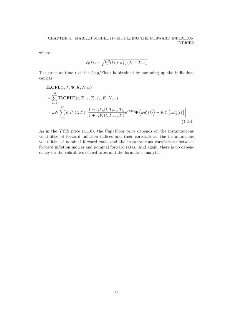
Where ETi denotes expectation under the (nominal) Ti forward measure. Theprice of the Inflation Linked Cap/Floor(ILCF) is obtained by summing up over theindividual Caplets/Florlets. Clearly this price is model dependent as well.

1.3 Inflation and interest rate risk

1.3.1 Breakeven inflation vs expected inflation

Compounding effect

It seems intuitive to think of break-even inflation rate as a measure of expected futureinflation. There are however, a number of problems with that assumption. The firstis a simple compounding effect. Denote the annualized inflation rate between t = 0and T as

i(0, T ) =[I(T )I0

]1/T

− 1 (1.3.1)

8

1.3. INFLATION AND INTEREST RATE RISK

By the definition of the breakeven-inflation rate and Jensens Inequality we have

[1 + b(0, T )]T = E[[1 + i(0, T )]T

]≥ [1 + E [i(0, T )]]T (1.3.2)

Hence, the break-even rate is an overestimation of future inflation.

Inflation risk premium

The second argument to why break-even rates can not be directly translated intoexpected inflation, is that nominal rates are thought to carry a certain inflation riskpremium. A risk averse bond investor would demand a premium(a higher yield) tocompensate for the scenario where realized inflation turns out to be higher thanexpected inflation.

Consider a risk-averse investor who wishes to obtain a real return. The investorcan either buy a T -maturity inflation linked bond, receiving a real rate of returnyr(0, T ) or a T -maturity nominal bond, receiving a nominal rate of return yn(0, T ).Assuming that both bonds are issued today, the real return on the nominal bond is

I0I(T )

[1 + yn(0, T )]T

whereas the real return for the index linked bond is

[1 + yr(0, T )]T

To compensate for the inflation risk, i.e. the scenario where realized inflation over[0, T ] turns out be greater than the expected inflation, the risk averse investorwould demand an additional return on yn, in effect demanding a higher yield thanmotivated by inflation expectations

[1 + yn(0, T )]T ≥ [1 + yr(0, T )]T E[I(T )I0

]= [1 + yr(0, T )]T E

[[1 + i(0, T )]T

]Denoting the inflation risk premium over [0, T ] as p(0, T ), we can express the nom-inal return as

[1 + yn(0, T )]T = [1 + p(0, T )]T [1 + yr(0, T )]T E[[1 + i(0, T )]T

]Consequently , break-even inflation rates will include the risk premium , i.e overes-timate future inflation rates.

Assuming a correction factor c(0, T ) ≥ 0 such that we can rewrite (1.3.2) as

E[[1 + i(0, T )]T

]= [1 + c(0, T )]T [1 + E [i(0, T )]]T (1.3.3)

, then we can express the nominal return in the style of the famous Fisher Equation

1 + yn(0, T ) = [1 + p(0, T )] [1 + yr(0, T )] [1 + c(0, T )] [1 + E [i(0, T )]] (1.3.4)

9


1.3.2 Inflation riskSince the annually compounded nominal yield yn is defined as

yn(t, T ) = Pn(t, T )−1/T − 1 (1.3.5)

by (1.2.5) and (1.2.16) we can write the price of an ILB in terms of the break-eveninflation curve and the nominal yield curve

ILB(t, TM , I0, N, sb, sn) = I(t)I0

N

[C

M∑i=1

(1 + b(t, Ti) + sb)Ti

(1 + yn(t, Ti) + sn)Ti+ (1 + b(t, TM ) + sb)TM

(1 + yn(t, TM ) + sn)TM

](1.3.6)

where sb and sn should equal zero in order for the price to be fair. Thus it’s clearthat the price is sensitive to shifts in the inflation curve as well as to shifts in thenominal interest curve.

The effect of a parallel shift in the nominal interest curve is then obtained as

∂ILB(t, TM , I0, N, 0, 0)∂sn

= −I(t)I0

N

[C

M∑i=1

TiPr(t, Ti)

1 + yn(t, Ti)+ TM

Pr(t, TM )1 + yn(t, TM )

](1.3.7)

And the effect of a parallel shift in the inflation curve as

∂ILB(t, TM , I0, N, 0, 0)∂sb

= I(t)I0

N

[C

M∑i=1

TiPr(t, Ti)

1 + b(t, Ti)+ TM

Pr(t, TM )1 + b(t, TM )

](1.3.8)

Since the inflation delta and the nominal yield delta have opposite signs, the neteffect will be small if the inflation and nominal curves are equally shifted. Typically,a rise in inflation expectation pushes up the nominal interest rates, so it’s naturalto impose some correlation ρn,I between the two, by - for instance - setting sb =sn × ρn,I . Indeed when modeling the evolution of interest rates and inflation in theshort rate model of Jarrow and Yildirim[1] and the market model of Mercurio[2]and Belgrade, Benhamou, and Koehler[4], a correlation structure is proposed in themodel dynamics.

10

Chapter 2

The HJM framework of Jarrow andYildirim

2.1 Definitions

Using a foreign currency analogy, Jarrow and Yildirim reasoned that real pricescorrespond to foreign prices, nominal prices correspond to domestic prices and theinflation index corresponds to the spot exchange rate from foreign to domesticcurrency. We introduce the notation which will be used throughout this section.

• Pn(t, T ) : time t price of a nominal zero coupon bond maturing at time T

• I(t): time t value of the inflation index

• Pr(t, T ) : time t price of a real zero-coupon bond maturing at time T

• fk(t, T ): time t instantaneous forward rate for date T where k ∈ r, n i.e.

Pk(t, T ) = e−∫ T

tfk(t,s)ds

• rk(t) = fk(t, t) : the time t instantaneous spot rate for k ∈ r, n

• Bk(t) : time t money market account value for k ∈ r, n

2.2 Model specification

Under the real world probability space (Ω,F , P ), Jarrow and Yildirim introducethe filtration Ft : t ∈ [0, T ] generated by the three brownian motions

dWPn (t), dWP

r (t), dWPI (t) (2.2.1)

11

CHAPTER 2. THE HJM FRAMEWORK OF JARROW AND YILDIRIM

The brownian motions are started at 0 and their correlations are given by

dWPn (t) dWP

r (t) = ρnrdt

dWPn (t) dWP

I (t) = ρnIdt

dWPr (t) dWP

I (t) = ρrIdt

(2.2.2)

Thus, we will be working with a three-factor model.Given the initial nominal forward rate curve, f∗

n(0, T ), it’s assumed that thenominal T -maturity forward rate has a stochastic differential under the objectivemeasure P given by

dfn(t, T ) = αn(t, T )dt+ σn(t, T )dWPn (t)

fn(0, T ) = f∗n(0, T )

(2.2.3)

where αn is random and σn is deterministic.Similarly, given the initial market real forward rate curve, f∗

r (0, T ), it’s assumedthat the real T -maturity forward rate has a stochastic differential under the objectivemeasure P given by

dfr(t, T ) = αr(t, T )dt+ σr(t, T )dWPr (t)

fr(0, T ) = f∗r (0, T )

(2.2.4)

where αn is random and σn is deterministic. The final entity to be modeled is theinflation index with dynamics

dI(t)I(t)

= µI(t)dt+ σI(t)dWPI (t) (2.2.5)

where µI is random and σI is deterministic. The deterministic volatility in (2.2.5)implies that the inflation index follows a geometric brownian motion so that thelogarithm of the index will be normally distributed.

Jarrow and Yildirim go on to show the evolutions introduced so far are arbi-trage free and the market is complete if there exists a unique equivalent probabilitymeasure Q such that

Pn(t, T )Bn(t)

,I(t)Pr(t, T )

Bn(t)and I(t)Br(t, T )

Bn(t)are Q martingales (2.2.6)

Furthermore, by Girsanov’s theorem, given that dWPn (t), dWP

r (t), dWPI (t) is a

P -Brownian motion, and that Q is a equivalent probability measure, then thereexists market prices of risk λn(t), λr(t), λI(t) such that

WQk (t) = WP

k (t) −∫ t

0λk(s)ds, k ∈ n, r, I (2.2.7)

are Q-brownian motions.Finally, they provided the following proposition, which characterizes the neces-

sary and sufficient conditions on the various price dynamics such that the economyis arbitrage free.

12

2.2. MODEL SPECIFICATION

Proposition 2.2.1 (Arbitrage Free Term Structure)Pn(t,T )Bn(t) , I(t)Pr(t,T )

Bn(t) and I(t)Br(t,T )Bn(t) are Q martingales if and only if

αn(t, T ) = σn(t, T )(∫ T

tσn(t, s)ds− λn(t)

)(2.2.8)

αr(t, T ) = σr(t, T )(∫ T

tσr(t, s)ds− σI(t)ρrI − λr(t)

)(2.2.9)

µI(t) = rn(t) − rr(t) − σI(t)λI(t) (2.2.10)

(2.2.8) is recognized as the well known HJM drift condition for the nominalforward rates under the objective probability measure. Analogously, (2.2.9) is thedrift condition for the real forward rates. It is to be noted that the inflation volatilityand the inflation-real rate correlation appears in this expression. Finally (2.2.10) isa fisher equation(compare with the heuristics in (1.3.4) ), relating nominal and realinterest rates to expected inflation(µI) and inflationary risk premium.

13


2.3 Zero Coupon Bond term structure

2.3.1 General formIt can be shown(see [5]) that, for k ∈ n, r, the log-bond price process can bewritten as

lnPk(t, T ) = −∫ T

tfk(t, u)du =

= lnPk(0, T ) −∫ t

0

[∫ T

vαk(v, u)du

]dv −

∫ t

0

[∫ T

vσk(v, u)du

]dWP

k (v)

+∫ t

0rk(v)dv

(2.3.1)

Let

ak(t, T ) = −∫ T

tσk(t, u)du (2.3.2)

bk(t, T ) = −∫ T

tαk(t, u)du+ 1

2a2

k(t, T ) (2.3.3)

Then we can write

lnPk(t, T ) = lnPk(0, T ) +∫ t

0[rk(v) + bk(v, T )] dv − 1

2

∫ t

0a2

k(v, T )dv

+∫ t

0ak(v, T )dWP

k (v)(2.3.4)

Or

d lnPk(t, T ) =[rk(t) + bk(t, T ) − 1

2a2

k(t, T )]dt+ ak(t, T )dWP

k (t) (2.3.5)

Applying Itô’s lemma yields the bond price process

dPk(t, T )Pk(t, T

= [rk(t) + bk(t, T )] dt+ ak(t, T )dWPk (t)

=[rk(t) −

∫ T

tαk(t, u)du+ 1

2a2

k(t, T )]dt+ ak(t, T )dWP

k (t)(2.3.6)

2.3.2 Jarrow Yildirim drift conditionsNominal bond price

We note that for the nominal drift condition

αn(t, u) = σn(t, u)(∫ u

tσn(t, s)ds− λn(t)

)= 1

2d(a2

n(t, u))

du+ d (an(t, u))

duλn(t)

(2.3.7)

14

2.3. ZERO COUPON BOND TERM STRUCTURE

So that with (2.3.6), under P , the dynamics of the nominal zero coupon bond isgiven as

dPn(t, T )Pn(t, T

= [rn(t) − an(t, T )λn(t)] dt+ an(t, T )dWPn (t) (2.3.8)

and under QdPn(t, T )Pn(t, T

= rn(t)dt+ an(t, T )dWQn (t) (2.3.9)

Real bond price

Similarly, for the real drift condition

αr(t, u) = σr(t, u)(∫ u

tσr(t, s)ds− σI(t)ρrI − λr(t)

)= 1

2d(a2

r(t, u))

du+ d (ar(t, u))

du[σI(t)ρrI + λr(t)]

(2.3.10)

So that under P the dynamics of the real zero coupon bond is given asdPr(t, T )Pr(t, T

= [rr(t) − ar(t, T ) σI(t)ρrI + λr(t)] dt+ ar(t, T )dWPr (t) (2.3.11)

and under QdPr(t, T )Pr(t, T

= [rr(t) − ar(t, T )σI(t)ρrI ] dt+ ar(t, T )dWQr (t) (2.3.12)

These results, and applying the drift conditions on the forward rates and the infla-tion index processes and integration by parts on the process I(t)Pr(t, T ), yields thefollowing proposition

Proposition 2.3.1 (Price processes under the martingale measure)The following price processes hold under the martingale measure

dfn(t, T ) = −σn(t, T )an(t, T )dt+ σn(t, T )dWQn (t) (2.3.13)

dfr(t, T ) = −σr(t, T ) [ar(t, T ) + ρrIσI(t)] dt+ σr(t, T )dWQr (t) (2.3.14)

dI(t)I(t)

= [rn(t) − rr(t)] dt+ σI(t)dWQI (t) (2.3.15)

dPn(t, T )Pn(t, T )

= rn(t)dt+ an(t, T )dWQn (t) (2.3.16)

dPr(t, T )Pr(t, T

= [rr(t) − ar(t, T )σI(t)ρrI ] dt+ ar(t, T )dWQr (t) (2.3.17)

dPIL(t, T )PIL(t, T )

:= d(I(t)Pr(t, T ))I(t)Pr(t, T )

= rn(t)dt+ σI(t)dWQI (t) + ar(t, T )dWQ

r (t) (2.3.18)

We note here that with these expressions, the nominal and real forward ratesare normally distributed, whereas the inflation index is log-normally distributed.

15


2.4 Hull-White specification

2.4.1 Nominal term structure

For the nominal economy, Jarrow and Yildirim chose a one factor volatility functionwith an exponentially declining volatility of the form

σn(t, T ) = σne−κn(T −t) (2.4.1)

This yields the zero coupon bond volatility as

an(t, T ) = −∫ T

tσn(t, u)du = −σn

∫ T

te−κn(u−t)du = −σnβn(t, T ) (2.4.2)

whereβn(t, T ) = 1

κn

[1 − e−κn(T −t)

](2.4.3)

and that the forward rate under Q evolves as

fn(t, T ) = fn(0, T ) + σ2n

∫ t

0βn(s, T )e−κn(T −s)ds+ σn

∫ t

0e−κn(T −s)dWQ

n (s) (2.4.4)

, the spot rate as

rn(t) = fn(t, t) = fn(0, t) + σ2n

∫ t

0βn(s, t)e−κn(t−s)ds+ σn

∫ t

0e−κn(t−s)dWQ

n (s)

= fn(0, t) + σ2n

2

∫ t

0

∂β2n(s, t)∂t

ds+ σn

∫ t

0e−κn(t−s)dWQ

n (s)

= fn(0, t) + σ2n

2∂

∂t

(∫ t

0β2

n(s, t)ds)

+ σn

∫ t

0e−κn(t−s)dWQ

n (s)

(2.4.5)

and∫ t

0rn(u)du = − lnPn(0, t) + σ2

n

2

∫ t

0β2

n(s, t)ds+∫ t

0

[σn

∫ u

0e−κn(u−s)dWQ

n (s)]du

(2.4.6)

We need to do some work in order to evaluate the double integral. Introducing theprocess Y (t) =

∫ t0 e

asdWQn (s) we have

d(e−atY (t)) = e−atdY (t) − ae−atY (t)dt = dWQn (t) − ae−atY (t)dt (2.4.7)

Integrating, we get

e−atY (t) = WQn (t) −

∫ t

0ae−auY (u)du (2.4.8)

16

2.4. HULL-WHITE SPECIFICATION

Inserting the definition of Y (·) in the expression above yields

a

∫ t

0

[e−au

∫ u

0easdWQ

n (s)]du = WQ

n (t) − e−at∫ t

0eaudWQ

n (u)

=∫ t

0

(1 − e−a(t−u)

)dWQ

n (u)

= a

∫ t

0β(u, t)dWQ

n (u)

(2.4.9)

Applying the result above in (2.4.6), we get∫ t

0rn(u)du = − lnPn(0, t) + σ2

n

2

∫ t

0β2

n(s, t)ds+ σn

∫ t

0βn(s, t)dWQ

n (s) (2.4.10)

Substituting this in the solution to the zero coupon bond price process yields

Pn(t, T ) = Pn(0, T ) exp∫ t

0

(rn(s) − a2

n(s, T )2

)ds+

∫ t

0an(s, T )dWQ

n (s)

= Pn(0, T ) exp∫ t

0

(rn(s) − σ2

n

2β2

n(s, T ))ds− σn

∫ t

0βn(s, T )dWQ

n (s)

= Pn(0, T )Pn(0, t)

expσ2

n

2

∫ t

0

[β2

n(s, t) − β2n(s, T )

]ds+ σn

∫ t

0[βn(s, t) − βn(s, T )] dWQ

n (s)

(2.4.11)

Noting from (2.4.5) that

−βn(t, T )rn(t) = −βn(t, T )fn(0, t) + σ2n

∫ t

0

[β2

n(s, t) − βn(s, T )βn(s, t)]ds

+ σn

∫ t

0[βn(s, t) − βn(s, T )] dWQ

n (s)(2.4.12)

, then the term inside the exponential in (2.4.11) simplifies to

βn(t, T ) [fn(0, t) − rn(t)]

− σ2n

2

∫ t

0

[β2

n(s, t) + β2n(s, T ) − 2βn(s, T )βn(s, t)

]ds

= βn(t, T ) [fn(0, t) − rn(t)] − σ2n

2

∫ t

0[βn(s, t) − βn(s, T )]2 ds

= βn(t, T ) [fn(0, t) − rn(t)] − σ2n

4κnβ2

n(t, T )[1 − e−2κnt

](2.4.13)

So that we get the nominal term structure in terms of the short rate

Pn(t, T ) = Pn(0, T )Pn(0, t)

expβn(t, T ) [fn(0, t) − rn(t)] − σ2

n

4κnβ2

n(t, T )[1 − e−2κnt

](2.4.14)

17


2.4.2 Real term structure

For the real economy, Jarrow and Yildirim chose again chose we a one factor volatil-ity function with an exponentially declining volatility of the form

σr(t, T ) = σre−κr(T −t) (2.4.15)

This yields the real zero coupon bond volatility as

ar(t, T ) = −∫ T

tσr(t, u)du = −

∫ T

tσre

−κr(u−t)du = −σrβr(t, T ) (2.4.16)

whereβr(t, T ) = 1

κr

[1 − e−κr(T −t)

](2.4.17)

For the inflation index process we assume a constant volatility, σI . Similar calcula-tions as in the previous section then renders the real term structure as

Pr(t, T ) = Pr(0, T )Pr(0, t)

expσ2

r

2

∫ t

0

[β2

r (s, t) − β2r (s, T )

]ds+ σr

∫ t

0[βr(s, t) − βr(s, T )]dWQ

r (s)s

× exp

−ρrIσIσr

∫ t

0[βr(s, t) − βr(s, T )]ds

(2.4.18)

or in terms of the real short rate

Pr(t, T ) = Pr(0, T )Pr(0, t)

expβr(t, T ) [fr(0, t) − rr(t)] − σ2

r

4κrβ2

r (t, T )[1 − e−2κrt

](2.4.19)

2.5 Year-On-Year Inflation SwapIt turns out that it’s convenient to derive the price of the inflation leg under theT -forward measure. By (1.2.21) and a change of measure we get

YYIIS(t, Ti−1, Ti, ψi, N) = Nψi

(Pn(t, Ti−1)ETi−1 [Pr(Ti−1, Ti)| Ft] − Pn(t, Ti)

)(2.5.1)

So we need to work out the dynamics of Pr(t, T2) under the T1-forward measure.Applying the toolkit specified in Proposition (A.1.1) in (2.3.17), we get the followingdynamics for Pr(t, T2) under the T1-forward measure

dPr(t, T2)Pr(t, T2)

= [rr(t) − ar(t, T2)σI(t)ρrI + ar(t, T2)an(t, T1)ρnr] dt+ ar(t, T1)dW T1r (t)

(2.5.2)

18

2.5. YEAR-ON-YEAR INFLATION SWAP

with solution

Pr(t, T2) = Pr(0, T2) exp∫ t

0(rr(s) − ar(s, T2)σI(s)ρrI + ar(s, T2)an(s, T1)ρnr) ds

× exp

−∫ t

0

a2r(s, T2)

2ds+

∫ t

0ar(s, T2)dW T1

r (s)

(2.5.3)

And after some straightforward calculations we find that

Pr(t, T2)Pr(t, T1)

= Pr(0, T2)Pr(0, T1)

E(∫ t

0[ar(s, T2) − ar(s, T1)] dW T1

r (s))

× exp∫ t

0[ar(s, T2) − ar(s, T1)] [an(s, T1)ρnr − σI(s)ρrI − ar(s, T1)] ds

(2.5.4)

where E denotes the Doléans-Dade exponential, defined as

E(X(t)) = expX(t) − 1

2⟨X,X⟩ (t)

(2.5.5)

So that, with t = T1 we get

Pr(T1, T2) = Pr(0, T2)Pr(0, T1)

E(∫ T1

0[ar(s, T2) − ar(s, T1)] dW T1

r (s))

× exp∫ T1

0[ar(s, T2) − ar(s, T1)] [an(s, T1)ρnr − σI(s)ρrI − ar(s, T1)] ds

(2.5.6)

Or

Pr(T1, T2) | Ft = Pr(t, T2)Pr(t, T1)

E(∫ T1

t[ar(s, T2) − ar(s, T1)] dW T1

r (s))

× eC(t,T1,T2)

(2.5.7), where

C(t, T1, T2) =∫ T1

t[ar(s, T2) − ar(s, T1)] [an(s, T1)ρnr − σI(s)ρrI − ar(s, T1)] ds

(2.5.8)Hence

ET1 [Pr(T1, T2) | Ft] = Pr(t, T2)Pr(t, T1)

eC(t,T1,T2) (2.5.9)

So we see that the expectation of the future real zero bond price under the nominalforward measure is equal to the current forward price of the real bond, multipliedby a correction factor. The factor depends on the volatilities and correlations of the

19


nominal rate, the real rate and the inflation index. Applying (2.5.9) in (2.5.1) givesus

YYIIS(t, Ti−1, Ti, ψi, N) = Nψi

[Pn(t, Ti−1) Pr(t, Ti)

Pr(t, Ti−1)eC(t,Ti−1,Ti) − Pn(t, Ti)

](2.5.10)

Straightforward calculations shows that the correction term can be explicitly com-puted as

C(t, Ti−1, Ti) = σrβr(Ti−1, Ti)[βr(t, Ti−1)

(ρr,IσI − 1

2βr(t, Ti−1)

+ ρn,rσn

κn + κr(1 + κrβn(t, Ti−1))

)− ρn,rσn

κn + κrβn(t, Ti−1)

] (2.5.11)

This term accounts for the stochasticity of real rates. Indeed it vanishes for σr = 0.The time t value of the inflation linked leg is obtained by summing up the values

of all payments.

YYIIS(t, T ,Ψ, N) = Nψι(t)

[I(t)

I(Tι(t)−1)Pr(t, Tι(t)) − Pn(t, Tι(t))

]

+NM∑

i=ι(t)+1ψi


Pr(t, Ti−1)eC(t,Ti−1,Ti) − Pn(t, Ti)

](2.5.12)

where we set T := T1, · · · , TM , Ψ := ψ1, · · · , ψM , ι(t) = min i : Ti > t andwhere the first cash flow has been priced according to the zero coupon inflation legformula derived in (1.2.13). Speficially, at t = 0

YYIIS(0, T ,Ψ, N) = Nψ1 [Pr(0, T1) − Pn(0, T1)]

+NM∑

i=2ψi

[Pn(0, Ti−1) Pr(0, Ti)

Pr(0, Ti−1)eC(0,Ti−1,Ti) − Pn(0, Ti)

](2.5.13)

The advantage of the Jarrow-Yildirim model is the simple closed formula it resultsin. However, the dependence on the real rate parameters, such as the volatility ofreal rates is a significant drawback, as it is not easily estimated.

2.6 Inflation Linked Cap/FloorWe recall that the inflation index, I(t), is log-normally distributed under Q. Underthe nominal forward measure, the inflation index I(Ti)

I(Ti−1) preserves a log-normaldistribution. Thus, (1.2.23) can be calculated when we know the expectation of the

20

2.6. INFLATION LINKED CAP/FLOOR

ratio and the variance of it’s logarithm. Using the fact that if X is a log-normallydistributed random variable with E[X] = m and Std[ln(X)] = v then

E[[ω (X −K)]+

]= ωmΦ

(ω

ln mK + 1

2v2

v

)− ωKΦ

(ω

ln mK − 1

2v2

v

)(2.6.1)

The conditional expectation of I(Ti)/I(Ti−1) is obtained directly from (1.2.19) and(2.5.10)

ETi

[I(Ti)I(Ti−1)

∣∣∣∣Ft

]= Pn(t, Ti−1)

Pn(t, Ti)Pr(t, Ti)Pr(t, Ti−1)

eC(t,Ti−1,Ti) (2.6.2)

Since a change of measure has no impact on the variance, it can be equivalentlycalculated under the martingale measure. By standard calculations it can then beshown that

VarTi

[ln I(Ti)I(Ti−1)

∣∣∣∣Ft

]= V 2(t, Ti−1, Ti) (2.6.3)

, where

V 2(t, Ti−1, Ti) = σ2n

2κnβ2

n(Ti−1, Ti)[1 − e−2κn(Ti−1−t)

]+ σ2

I (Ti − Ti−1)

+ σ2r

2κrβ2

r (Ti−1, Ti)[1 − e−2κr(Ti−1−t)

]− 2ρnr

σnσr

(κn + κr)βn(Ti−1, Ti)βr(Ti−1, Ti)

[1 − e−(κn+κr)(Ti−1−t)

]+ σ2

n

κ2n

[Ti − Ti−1 + 2

κne−κn(Ti−Ti−1) − 1

2κne−2κn(Ti−Ti−1) − 3

2κn

]+ σ2

r

κ2r

[Ti − Ti−1 + 2

κre−κr(Ti−Ti−1) − 1

2κre−2κr(Ti−Ti−1) − 3

2κr

]− 2ρnr

σnσr

κnκr

[Ti − Ti−1 − βn(Ti−1, Ti) − βr(Ti−1, Ti) + 1 − e−(κn+κr)(Ti−Ti−1)

κn + κr

]+ 2ρnI

σnσI

κn[Ti − Ti−1 − βn(Ti−1, Ti)] − 2ρrI

σrσI

κr[Ti − Ti−1 − βr(Ti−1, Ti)]

(2.6.4)

The quantities derived in this section then yields the Caplet/Floorlet price as

ILCFLT(t, Ti−1, Ti, ψi,K,N, ω) =

ωNψiPn(t, Ti)[Pn(t, Ti−1)Pn(t, Ti)

Pr(t, Ti)Pr(t, Ti−1)

eC(t,Ti−1,Ti)Φ(ωdi

1(t))

−KΦ(ωdi

2(t))]

di1(t) =

ln Pn(t,Ti−1)KPn(t,Ti)

Pr(t,Ti)Pr(t,Ti−1) + C(t, Ti−1, Ti) + 1

2V2(t, Ti−1, Ti)

V (t, Ti−1, Ti)di

2(t) = d1 − V (t, Ti−1, Ti)(2.6.5)

21


Just as for the year-on-year inflation swap, the price depends on the volatility ofreal rates. In the following sections we will present two market models that havebeen proposed as an alternative for valuation of inflation linked instruments. Themodels strive to arrive at valuation formulas , where the input parameters are moreeasily determined than in the short rate approach of the Jarrow-Yildirim model.

22

Chapter 3

Market Model I - A Libor Market Modelfor nominal and real forward rates

3.1 Year-On-Year Inflation SwapBy a change of measure, the expectation in (1.2.21) can be rewritten as

Pn(t, Ti−1)ETi−1 [Pr(Ti−1, Ti)| Ft] = Pn(t, Ti)ETi

[Pr(Ti−1, Ti)Pn(Ti−1, Ti)

∣∣∣∣Ft

]= Pn(t, Ti)ETi

[ 1 + τi · Fn(Ti−1, Ti−1, Ti)1 + τi · Fr(Ti−1, Ti−1, Ti)

∣∣∣∣Ft

] (3.1.1)

where τi denotes year fraction between Ti−1 and Ti and Fk : k ∈ n, r denotesthe simply compounded forward rate. The expectation can be evaluated if weknow the distribution of simply compounded nominal and real forward rates underthe nominal Ti-forward measure. This inspired Mercurio[2] to choose them as thequantities to model, with the following dynamics under QTi

n

dFn(t, Ti−1, Ti)Fn(t, Ti−1, Ti)

= σn,idWn,i(t) (3.1.2)

And under QTir

dFr(t, Ti−1, Ti)Fr(t, Ti−1, Ti)

= σr,idWr,i(t) (3.1.3)

To obtain the dynamics of the real forward rate under QTin , we compute the drift

adjustment using Proposition (A.1.1) to find that under QTin

dFr(t, Ti−1, Ti)Fr(t, Ti−1, Ti)

= −σr,iσI,iρI,r,idt+ σr,idWr,i(t) (3.1.4)

where σn,i and σr,i are positive constants and ρI,r,i is the instantaneous correlationbetween I(·, Ti) and Fr(·, Ti−1, Ti).

23

CHAPTER 3. MARKET MODEL I - A LIBOR MARKET MODEL FOR NOMINALAND REAL FORWARD RATES

Since I(t)Pr(t, T ) is the price of the inflation linked bond, which is a tradedasset in the nominal economy, it holds that the forward inflation index

I(t, Ti) = I(t)Pr(t, Ti)Pn(t, Ti)

(3.1.5)

is a martingale under QTin , where it is proposed to follow log-normal dynamics

dI(t, Ti)I(t, Ti)

= σI,idWI,i(t) (3.1.6)

where σI,i is a positive constant and WI,i is a QTin brownian motion.

Mercurio noted that under QTin and conditional on Ft the pair

(Xi, Yi) =(

ln Fn(Ti−1, Ti−1, Ti)Fn(t, Ti−1, Ti)

, ln Fr(Ti−1, Ti−1, Ti)Fr(t, Ti−1, Ti)

)(3.1.7)

is distributed as a bivariate normal random variable with mean vector and covari-ance matrix, respectively given by

MXi,Yi =[µx,i(t)µy,i(t)

], VXi,Yi =

[σ2

x,i(t) ρn,r,iσx,i(t)σy,i(t)ρn,r,iσx,i(t)σy,i(t) σ2

y,i(t)

](3.1.8)

where

µx,i(t) = −12σ2

n,i(Ti−1 − t), σx,i(t) = σn,i

√(Ti−1 − t)

µy,i(t) =[−1

2σ2

r,i − ρI,r,iσI,iσr,i

](Ti−1 − t), σy,i(t) = σr,i

√(Ti−1 − t)

We recall the fact that the bivariate density fXi,Yi(x, y) of (Xi, Yi) can be decom-posed in terms of the conditional density fXi|Yi

(x, y) as

fXi,Yi(x, y) = fXi|Yi(x, y)fYi(y)

where

fXi|Yi(x, y) = 1

σx,i(t)√

2π√

1 − ρ2n,r,i

exp

−

[x−µx,i(t)

σx,i(t) − ρn,r,iy−µy,i(t)

σy,i(t)

]22(1 − ρ2

n,r,i)

fYi(y) = 1

σy,i(t)√

2πexp

−12

[y − µy,i(t)σy,i(t)

]2

Noting that

Fn(Ti−1, Ti−1, Ti) = eXiFn(t, Ti−1, Ti)Fr(Ti−1, Ti−1, Ti) = eYiFr(t, Ti−1, Ti)

24

3.1. YEAR-ON-YEAR INFLATION SWAP

, the expectation in (3.1.1) can be calculated as∫ +∞

−∞

∫+∞−∞ (1 + τiFn(t, Ti−1, Ti)ex)fXi|Yi

(x, y)dx1 + τiFr(t, Ti−1, Ti)ey

fYi(y)dy

=∫ +∞

−∞

1 + τiFn(t, Ti−1, Ti)eµx,i(t)+ρn,r,iσx,i(t)

y−µy,i(t)σy,i(t) + 1

2 σ2x,i(t)[1−ρ2

n,r,i]

1 + τiFr(t, Ti−1, Ti)eyfYi(y)dy

=

by µx,i(t) = −12σ2

x,i(t) and variable substitution z = y − µy,i(t)σy,i(t)

=∫ +∞

−∞

1 + τiFn(t, Ti−1, Ti)eρn,r,iσx,i(t)z− 12 σ2

x,i(t)ρ2n,r,i

1 + τiFr(t, Ti−1, Ti)eµy,i(t)+σy,i(t)z1√2πe− 1

2 z2dz

so that

YYIS(t, Ti−1, Ti, ψi, N)

= NψiPn(t, Ti)∫ +∞

−∞


x,i(t)ρ2n,r,i


2 z2dz

−NψiPn(t, Ti)(3.1.9)

Some care needs to be taken when valuing the whole inflation leg. We can’t simplysum up the values in (3.1.9). To see this, note that by (3.1.5) and the assumptionof simply compounded rates we have

I(t, Ti)I(t, Ti−1)

= 1 + τiFn(t, Ti−1, Ti)1 + τiFr(t, Ti−1, Ti)

(3.1.10)

Thus, if we assume that σI,i, σn,i and σr,i are positive constants then σI,i−1 cannotbe constant as well. It’s admissable values are obtained by equating the quadraticvariations on both side of (3.1.10). For instance, if nominal and real forward ratesas well as the forward inflation index were driven by the same brownian motion,then equating the quadriatic variations in (3.1.10) yields

σI,i−1 = σI,i + σr,iτiFr(t, Ti−1, Ti)

1 + τiFr(t, Ti−1, Ti)− σn,i

τiFn(t, Ti−1, Ti)1 + τiFn(t, Ti−1, Ti)

Mercurio applied a "freezing procedure" where the forward rates in the diffusioncoefficient on the right hand side of (3.1.10) are frozen at their time 0 value, so thatwe can still get forward inflation index volatilities that are approximately constant.In the case where all processes are driven by the same brownian motion, equatingthe quadratic variations would yield

σI,i−1 ≈ σI,i + σr,iτiFr(0, Ti−1, Ti)

1 + τiFr(0, Ti−1, Ti)− σn,i

τiFn(0, Ti−1, Ti)1 + τiFn(0, Ti−1, Ti)

25


Thus, applying this approximation for each i, we can still assume that the volatil-ities σI,i are all constant. The time t value of the inflation leg is then given by

YYIIS(t, T ,Ψ, N) = Nψι(t)

[I(t)


]

+NM∑

ι(t)+1ψiPn(t, Ti) ×

∫ +∞

−∞


x,i(t)ρ2n,r,i


2 z2dz − 1

(3.1.11)

where we set T := T1, · · · , TM , Ψ := ψ1, · · · , ψM , ι(t) = min i : Ti > t andwhere the first cash flow has been priced according to the zero coupon inflation legformula derived in (1.2.13).

At t = 0 we get

YYIIS(0, T ,Ψ, N) = Nψ1 [Pr(0, T1) − Pn(0, T1)]

+NM∑2ψiPn(0, Ti) ×

∫ +∞

−∞

1 + τiFn(0, Ti−1, Ti)eρn,r,iσx,i(0)z− 12 σ2

x,i(0)ρ2n,r,i

1 + τiFr(0, Ti−1, Ti)eµy,i(0)+σy,i(0)z1√2πe− 1

2 z2dz − 1

= N

M∑1ψiPn(0, Ti) ×

∫ +∞

−∞

1 + τiFn(0, Ti−1, Ti)eρn,r,iσx,i(0)z− 12 σ2

x,i(0)ρ2n,r,i

1 + τiFr(0, Ti−1, Ti)eµy,i(0)+σy,i(0)z1√2πe− 1

2 z2dz − 1

(3.1.12)

The price depends on the following parameters: the instantaneous volatilities ofnominal and real forward rates and their correlations for each payment time Ti :1 < i <= M; and the volatilities of forward inflation indices and their correlationswith real forward rates for each payment time Ti : 1 < i <= M.

This formula looks looks more complicated than (2.5.12) both in terms of inputparameters and the calculations involved. Even with approximations made, we failto arrive at a closed-form valuation formula for a benchmark inflation derivative.And as in the Jarrow and Yilidrim model, the price depends on a number of realrate parameters that may be difficult to estimate.

3.2 Inflation Linked Cap/FloorApplying iterated expectation on (1.2.23) we get


= NψiPn(t, Ti)ETi

[[ω

(I(Ti)I(Ti−1)

−K

)]+∣∣∣∣∣Ft

]

= NψiPn(t, Ti)ETi

[ETi

[[ω

(I(Ti)I(Ti−1)

−K

)]+∣∣∣∣∣FT −1

]∣∣∣∣∣Ft

]

= NψiPn(t, Ti)ETi

[ 1I(Ti−1)

ETi

[[ω (I(Ti) − I(Ti−1)K)]+

∣∣∣FT −1]∣∣∣Ft

](3.2.1)

26


It is clear the the evaluation of the outer expectation depends on if one modelsthe forward inflation index(as presented in Market Model II), or the forward rates,which is the approach of Market Model I.

Assuming log-normal dynamics of the forward inflation index as defined in(3.1.6) and using that I(Ti) = I(Ti, Ti), yields the inner expectation as

ETi

[[ω (I(Ti) −KI(Ti−1))]+

∣∣∣FT −1]

= ETi

[[ω (I(Ti, Ti) −KI(Ti−1, Ti−1))]+

∣∣∣FT −1]

= ωI(Ti−1, Ti)Φ

ω ln I(Ti−1,Ti)KI(Ti−1,Ti−1) + 1

2σ2I,i(Ti − Ti−1)

σI,i√Ti − Ti−1

− ωKI(Ti−1)Φ

ω ln I(Ti−1,Ti)KI(Ti−1,Ti−1) − 1



Hence


= ωNψiPn(t, Ti)ETi

I(Ti−1, Ti)I(Ti−1, Ti−1)

Φ

ω ln I(Ti−1,Ti)KI(Ti−1,Ti−1) + 1



−KΦ

ω ln I(Ti−1,Ti)KI(Ti−1,Ti−1) − 1



∣∣∣∣∣∣Ft

(3.2.2)

And by the definition of I(Ti−1, Ti−1) in (3.1.5), and the choice to model simplycompounded real and nominal forward rates, we note that

I(Ti−1, Ti)I(Ti−1, Ti−1)

= 1 + τiFn(Ti−1, Ti−1, Ti)1 + τiFr(Ti−1, Ti−1, Ti)

(3.2.3)

, so that we get the Caplet/Floorlet price as



[ 1 + τiFn(Ti−1, Ti−1, Ti)1 + τiFr(Ti−1, Ti−1, Ti)

Φ(ωdi

1(t))

−KΦ(ωdi

2(t))∣∣∣∣Ft

]

di1(t) =

ln 1+τiFn(Ti−1,Ti−1,Ti)K[1+τiFr(Ti−1,Ti−1,Ti)] + 1



di2(t) = di

1(t) − σI,i

√(Ti − Ti−1)

(3.2.4)

We recall the assumption that nominal and real forward rates evolve accordingto (3.1.2) and (3.1.4) and utilize Mercurios freezing procedure described earlier,yielding constant forward inflation index volatilities volatilities. Again we use that,

27


under these assumptions, the pair (3.1.7) is distributed as a bivariate normal randomvariable with mean vector and covarience matrix given by (3.1.8). And so we canevaluate the expectation in (3.2.4).

The dimensionality of the problem can be reduced by assuming deterministicreal rates. As a consequence, the future rate Fr(Ti−1, Ti−1, Ti) is simply equal tothe current forward rate Fr(t, Ti−1, Ti), so that we can write the Caplet/Floorletprice as



[ 1 + τiFn(Ti−1, Ti−1, Ti)1 + τiFr(t, Ti−1, Ti)

Φ(ωdi

1(t))

−KΦ(ωdi

2(t))∣∣∣∣Ft

](3.2.5)

And since the nominal forward rate Fn(·, Ti−1, Ti) evolves as specified in (3.1.2), wehave


= ωNψiPn(t, Ti)∫ ∞

−∞J(x) 1

σn,i

√2π(Ti−1 − t)

e− 1

2

(x+ 1

2 σ2n,i(Ti−1−t)

σn,i√

Ti−1−t

)2

dx(3.2.6)

where

J(x) := 1 + τiFn(t, Ti−1, Ti)ex

1 + τiFr(t, Ti−1, Ti)Φ

ω ln 1+τiFn(t,Ti−1,Ti)ex

K[1+τiFr(t,Ti−1,Ti)] + 12σ

2I,i(Ti − Ti−1)


−KΦ

ω ln 1+τiFn(t,Ti−1,Ti)ex

K[1+τiFr(t,Ti−1,Ti)] − 12σ

2I,i(Ti − Ti−1)


The time 0 price of the Inflation Indexed Cap/Floor is then obtained by summingup the respective caplets/floorlets

ILCF(0, T ,Ψ,K,N, ω) =M∑

i=1ILCFT(0, Ti−1, Ti, ψi,K,N, ω)

= ωNψ1[Pr(0, T1)Φ

(ωdi

1(0))

−KPn(0, T1)Φ(ωdi

2(0))]

+ ωNM∑

i=2ψiPn(0, Ti)

∫ ∞

−∞J(0, x) 1

σn,i√

2πTi−1e

− 12

(x+ 1

2 σ2n,i

Ti−1σn,i

√Ti−1

)2

dx

(3.2.7)

The advantage of Market Model I, is that it is based on modeling observable quanti-ties, i.e. the individual forward rates. A clear disadvantage in comparison with theJarrow-Yildirim model is the , relatively, more complicated Caplet/Floorlet prices.Even though we made the unrealistic simplification that real rates are deterministic,we still end up with a "non closed-form" price formula.

28

Chapter 4

Market Model II - Modeling the forwardinflation indices

4.1 Year-On-Year Inflation SwapBoth the Jarrow-Yildirim Model and Market Model I share the drawback thatthey depend on the volatility of real rates, which might be a difficult parameter toestimate. To remedy this, a second market model has been proposed by Mercurio[2]and Belgrade, Benhamou, and Koehler[4]. In Market Model I, Mercurio modeledthe respective nominal and real forward rates for each forward date Ti. The coreproperty of Market Model II is the choice to model each respective forward inflationindex I(·, Ti).

Using that I(Ti) = I(Ti, Ti) and that I(t, Ti) is a martingale under QTin we can

write, for t < Ti−1

YYIIS(t, Ti−1, T, ψi, N) = NψiPn(t, Ti)ETi

[I(Ti)I(Ti−1)

− 1∣∣∣∣Ft

]= NψiPn(t, Ti)ETi

[ I(Ti, Ti)I(Ti−1, Ti−1)

− 1∣∣∣∣Ft

]= NψiPn(t, Ti)ETi

[ I(Ti−1, Ti)I(Ti−1, Ti−1)

− 1∣∣∣∣Ft

] (4.1.1)

The dynamics of I(t, Ti) under QTin is given by (3.1.6). Applying the toolkit in

proposition (A.1.1) yields the dynamics of I(t, Ti−1) under QTin as

dI(t, Ti−1)I(t, Ti−1)

= σI,i−1

[−τiσn,iFn(t, Ti−1, Ti)

1 + Fn(t, Ti−1, Ti)ρI,n,idt+ dWI,i−1(t)

](4.1.2)

where σI,i−1 is a positive constant, WI,i−1 is a QTin -Brownian motion with

dWI,i−1(t)dWI,i(t) = ρI,idt

29

CHAPTER 4. MARKET MODEL II - MODELING THE FORWARD INFLATIONINDICES

and ρI,n,i is the instantaneous correlation between I(·, Ti−1) and Fn(·, Ti−1, Ti)We see that the dynamics of I(·, Ti−1) underQTi

n depends on the nominal forwardrate Fn(t, Ti−1, Ti). To simplify the calculation in (4.1.1), Mercurio proposed tofreeze the drift in (4.1.2) at it’s current time t value. By this freezing procedureI(Ti−1, Ti−1)|Ft is lognormally distributed also under QTi

n . And since integrationby parts on d I(t,Ti)

I(t,Ti−1) yields

dI(t, Ti)

I(t, Ti−1)= σI,i−1

[τiσn,iFn(t, Ti−1, Ti)1 + Fn(t, Ti−1, Ti)

ρI,n,i + σI,i−1 − σI,iρI,i

]dt

+ σI,i−1dWI,i−1(t) + σI,idWI,i(t)(4.1.3)

, freezing the drift at it’s time-t value and noting the resulting log-normality ofI(t,Ti)

I(t,Ti−1) , enables us to calculate the expectation in (4.1.1) as

ETin

[ I(Ti−1, Ti)I(Ti−1, Ti−1)

∣∣∣∣Ft

]= I(t, Ti)

I(t, Ti−1)eDi(t)

where

Di(t) = σI,i−1

[τiσn,iFn(t, Ti−1, Ti)1 + τiFn(t, Ti−1, Ti)

ρI,n,i + σI,i−1 − σI,iρI,i

](Ti−1 − t)

Thus

YYIIS(t, Ti−1, Ti, ψi, N) = NψiPn(t, Ti)[ I(t, Ti)

I(t, Ti−1)eDi(t) − 1

]= NψiPn(t, Ti)

[Pn(t, Ti−1)Pr(t, Ti)Pr(t, Ti−1)Pn(t, Ti)

eDi(t) − 1] (4.1.4)

And we get the value of the inflation leg as

YYIIS(t, T ,Ψ, N) = Nψι(t)Pn(t, Tι(t))[

I(t, Tι(t))I(Tι(t)−1)

− 1]

+NM∑

i=ι(t)+1ψiPn(t, Ti)

[ I(t, Ti)I(t, Ti−1)

eDi(t) − 1]

= Nψι(t)

[I(t)


]

+NM∑

i=ι(t)+1ψi


Pr(t, Ti−1)eDi(t) − Pn(t, Ti)

](4.1.5)

where we set T := T1, · · · , TM , Ψ := ψ1, · · · , ψM , ι(t) = min i : Ti > t andwhere the first cash flow has been priced according to the zero coupon inflation leg

30


formula derived in (1.2.13). In particular at t = 0

YYIIS(0, T ,Ψ, N) = NM∑

i=1ψiPn(0, Ti)

[ I(0, Ti)I(0, Ti−1)

eDi(0) − 1]

= Nψ1 [Pr(0, T1) − Pn(0, T1)]

+NM∑

i=2ψi

[Pn(0, Ti−1) Pr(0, Ti)

Pr(0, Ti−1)eDi(0) − Pn(0, Ti)

]

= NM∑

i=1ψi Pn(0, Ti)

[1 + τiFn(0, Ti−1, Ti)1 + τiFr(0, Ti−1, Ti)

eDi(0) − 1]

(4.1.6)

This expression above has the advantage of using a market model approach com-bined with yielding a fully analytical formula. In addition, contrary to MarketModel I, the correction term does not depend on the volatility of real rates.

A drawback of the formula is that the approximation used when freezing thedrift may be rough for longer maturities. In fact, the formula above is exact onlywhen the correlations between I(·, Ti−1) and Fn(·, Ti−1, Ti) are assumed to be zeroso that the nominal forward rate is zeroed out from Di.

4.2 Inflation Linked Cap/FloorFrom (4.1.3) and again freezing the drift at it’s time t value, we obtain

ln I(Ti−1, Ti)I(Ti−1, Ti−1)

∣∣∣∣Ft ∼ N

( I(t, Ti)I(t, Ti−1)

+Di(t) − V 2i (t), V 2

i (t))

(4.2.1)

whereVi(t) :=

√[σ2

I,i−1 + σ2I,i − 2ρI,iσI,i−1σI,i

][Ti−1 − t] (4.2.2)

Choosing to model the forward inflation-index in (3.2.1) then yields


= ωNψiPn(t, Ti)

I(t, Ti)I(t, Ti−1)

eDi(t)Φ

ω ln I(t,Ti)KI(t,Ti−1) +Di(t) + 1

2V2i (t)

Vi(t)

−KΦ

ω ln I(t,Ti)KI(t,Ti−1) +Di(t) − 1

2V2i (t)

Vi(t)

= ωNψiPn(t, Ti)

[1 + τiFn(t, Ti−1, Ti)1 + τiFr(t, Ti−1, Ti)

eDi(t)Φ(ωdi

1(t))

−KΦ(ωdi

2(t))]

di1(t) =

ln 1+τiFn(t,Ti−1,Ti)K[1+τiFr(t,Ti−1,Ti)] +Di(t) + 1

2V2i (t)

Vi(t)di

2(t) = di1(t) − Vi(t)

(4.2.3)

31

CHAPTER 4. MARKET MODEL II - MODELING THE FORWARD INFLATIONINDICES

where

Vi(t) :=√V 2

i (t) + σ2I,i (Ti − Ti−1)

The price at time t of the Cap/Floor is obtained by summing up the individualcaplets

ILCFL(t, T ,Ψ,K,N, ω)

=M∑

i=1ILCFLT(t, Ti−1, Ti, ψi,K,N, ω)

= ωNM∑

i=1ψiPn(t, Ti)

[1 + τiFn(t, Ti−1, Ti)1 + τiFr(t, Ti−1, Ti)

eDi(t)Φ(ωdi

1(t))

−KΦ(ωdi

2(t))](4.2.4)

As in the YYIS price (4.1.6), the Cap/Floor price depends on the instantaneousvolatilities of forward inflation indices and their correlations, the instantaneousvolatilities of nominal forward rates and the instantaneous correlations betweenforward inflation indices and nominal forward rates. And again, there is no depen-dency on the volatilities of real rates and the formula is analytic.

32

Chapter 5

Calibration

5.1 Nominal- and Real Curves

0 5 10 15 20 25 30−1.5

−1

−0.5

0

0.5

1

1.5

2

2.5

Maturity(years)

Spo

t Rat

e(%

)

Nominal Zero−Coupon CurveReal Zero−Coupon Curve

Figure 5.1: Calibrated Euro Zero-Coupon Curves, 13 jul-2012

We need to extract the nominal zero-coupon rates, Pn(0, Ti) from the swapquotes, S(Ti), that we showed in Figure 1.1. The fixed leg on the EUR denominated

33

CHAPTER 5. CALIBRATION

0 5 10 15 20 25 30−1.5

−1

−0.5

0

0.5

1

1.5

2

2.5

3

Maturity(years)

6M F

orw

ard

Rat

e(%

)

Nominal Forward CurveReal Forward Curve

Figure 5.2: Calibrated Euro Forward Curves, 13 jul-2012

swaps rolls on a yearly basis, yielding the simple relation

S(Ti) = − 1 − P (0, Ti)∑ij=1 P (0, Tj)

(5.1.1)

, so that for all maturities Ti, i > 0, we can iteratively back out the zero-couponrates as

P (0, Ti) =1 − S(Ti)

∑i−1j=0 P (0, Tj)

1 + S(Ti)P (0, T0) = P (0, 0) := 1

(5.1.2)

To obtain the real zero-coupon rates, we take the break-even inflation rates, b(Ti),that we showed in Figure 1.1 and apply (1.2.16), i.e.

Pr(0, Ti) = Pn(0, Ti)(1 + b(Ti))Ti

The resulting nominal and real spot rates are shown in Figure 5.1. The correspond-ing forward rates are displayed in Figure 5.2.

34

5.2. SIMPLIFIED JARROW-YILDIRIM MODEL

5.2 Simplified Jarrow-Yildirim ModelAs a starting point for our calibration, we consider a simplistic model with thefollowing evolution of the inflation index

dI(t)I(t)

= [rn(t) − rr(t)] dt+ σIdWQI (t) (5.2.1)

where the nominal and real short rates, rn(.) and rr(.), are (unrealistically) assumedto be deterministic. And the inflation index volatility, σI , is constant. In this model,the Fisher equation is still preserved since.

EQ[I(T )I(t)

∣∣∣∣Ft

]= e

∫ T

trn(u)−ru(u)du (5.2.2)

Note that, by Proposition (2.3.1) , this model is equivilant to the Jarrow-Yildirimmodel with σn = σr = 0. Since there is then a 1-1 correspondence between Year-On-Year Floor price and implied volatility, we can recover the implied Floor volatilitysurface, as shown found in Figure 5.3.

The Floorlet volatility surface is constructed as follows. First, we construct theFloorlet prices by bootstrapping the quoted Year-On-Year Floor prices. Since weare only dependent on the inflation index volatility parameter, we may then - foreach Floorlet with expiry Ti and strike Ki - imply the corresponding inflation indexvolatility σTi,Ki . The result is displayed in Figure 5.4.

Clearly, the skew shape of the Floor surface and the rifled wing shape of theFloorlet surface indicates that the assumption of a single constant volatility is notrealistic. However, the simplistic model can still be of some use. When pricingInflation Caps/Floors, it can be utilized as a volatility parameter(by interpolatingin strike and expiry dimensions) to retrieve the appropriate volatility.

35


12

34

56

78

910

00.5

1.5

2.5

1

1.5

2

2.5

3

3.5

Strike(inflation rate)Maturity(years)

Impl

ied

Vol

atili

ty(%

)

Figure 5.3: EUR Year-On-Year Inflation Floor Volatilities, 13 jul-2012

36

5.2. SIMPLIFIED JARROW-YILDIRIM MODEL

123456789100

0.5

1.5

2.5

1

2

3

4

5

6


Impl

ied

Vol

atili

ty(%

)

Figure 5.4: EUR Year-On-Year Inflation Floorlet Volatilities, 13 jul-2012

37


5.3 Jarrow Yildirim Model

5.3.1 Calibrating nominal volatility parameters to ATM Cap volatilities

0 5 10 15 20 25 3030

40

50

60

70

80

90

Maturity(years)

AT

M V

olat

ility

(%)

ATM Cap Volatilitites

Figure 5.5: EUR ATM Cap Volatility Curve, 13 jul-2012

By the choice of nominal volatility function, pricing a nominal Cap under theJ-Y model renders the well known Hull-White Cap/Floor valuation formula. Wemay then estimate the nominal volatility parameters with the following scheme. Foreach maturity Ti, we observe the ATM Cap (Black) volatility quote, σATM

i , shownin figure 5.5, and the accompanying ATM strike level KATM

i . We can then fit thenominal volatility parameters κn, σn by performing a least squares optimizationover

CapHull-White(t, Ti, ψi,KATMi , σn, κn) − CapBlack(t, Ti, ψi,K

ATMi , σATM

i )

From the resulting theoretical Hull-White prices we then back out the implied Blackvolatility. The result is shown in Figure 5.6. The fit is not too bad in the long end ofthe curve. In the short end, we suffer from the limitations of our choice of nominalvolatility function. The exponentially declining form of volatility can not recover

38

5.3. JARROW YILDIRIM MODEL

the "hump" observed in the short end of the curve. However, note that although itwas the choice of Jarrow and Yildirim , the J-Y framework is not limited to Hull-White term structures. We are free to choose other volatility functions for a betterfit to Cap/Floor volatilities.

The implementation of nominal volatility structure calibration is a subject initself and is beyond the scope of this thesis. We simply point out that we are free tochoose a nominal volatility structure, other than that of Hull-White. For instance,had we set σn(t, T ) = σ then we would have rendered a Ho-Lee term structure.

1 3 5 7 9 11 13 15 17 19 21 23 25 27 290

50

100

150

200

250

Maturity(years)

Pric

e(ba

sis

poin

ts)

Market ATM VolatilitiesModel ATM Volatilities

Figure 5.6: EUR Market vs Model ATM Cap volatilities, 13 jul-2012

5.3.2 Fitting parameters to Year-On-Year Inflation Cap quotes

The remaining parameters to estimate are κr, σr, σI , ρnr, ρIr ρIn. All these param-eters enter the YoY inflation Cap/Floor valuation formula, so that we may attemptto calibrate to market prices. However, given the indicative shape of the volatilitysurface recovered in the previous section, we know that we cannot fit to the wholesurface. Removing the two OTM contracts at strike 0 and 0.5 still results in high

39


relative errors as shown in Figure 5.7. Excluding the longer dated contracts fromthe calibration (Figure 5.8), still results in a poor fit.

We conclude that we must restrict ourself to the (closest to) ATM contract andrestrict the expiry dimension to get a reasonable fit, as shown in figure in 5.9. The fitin the expiry dimension can be improved by choosing more sophisticated volatilityfunctions for the real rate and the inflation index. The presence of a "strike skew"however, makes calibration unfeasible for non ATM contracts.

1.5

2.5

12

34

56

78

910

−20

0

20

40

60


Rel

ativ

e E

rror

(%)

Figure 5.7: Relative Error, EUR Year-on-Year Inflation Floor Model Prices, 13jul-2012

40

5.3. JARROW YILDIRIM MODEL

1.5

2.5

12

34

56

−20

0

20

40


Rel

ativ

e E

rror

(%)

Figure 5.8: Relative Error, EUR Year-on-Year Inflation Floor Model Prices, 13jul-2012

41


1 2 3−3

−2

−1

0

1

2

3

4

Maturity(years)

Rel

ativ

e E

rror

(%)

Relative Error, Strike = 1.5%

Figure 5.9: Relative Error, EUR ATM Year-on-Year Inflation Floor J-Y ModelPrices, 13 jul-2012

42

5.4. MARKET MODEL II

5.4 Market Model II

5.4.1 Nominal volatility parametersFor each maturity Ti we need to estimate the volatility , σn,i, of the (simply com-pounded) nominal forward rate Fn(·, Ti). By the log-normal dynamics of Fn(·, Ti)we get an automatic calibration to the quoted (Black) cap volatility σATM

i .

5.4.2 Fitting parameters to Year-On-Year Inflation Cap quotesThe remaining parameters to estimate, for each each maturity Ti, i > 2, are

σI,i−1, σI,i, ρI,i, ρI,n,i

The fitting procedure is run iteratively. That is, σI,1 is directly obtained from the1-Year Floor, since it depends on no other unknown parameters. We then proceedto use least squares estimation to fit the rest of the parameters to the correspondingFloor prices. The resulting price error surface is plotted in Figure 5.10.

Since each expiry has it’s own set of parameters, there is no need to restrictthe number of contracts in the expiry dimension. The skew in the strike dimensionhowever, results in a poor fit if we want to include non ATM contracts. Fromthe figure, it’s clear that if we assume constant volatility in the expiry dimension,then OTM contracts are underpriced and ITM contracts are overpriced. As inthe J-Y model, we must restrict ourselves to (close to) ATM contracts to recovermarket prices. Or alternatively, take the "practitioners approach" and imply a setof parameters for each Expiry/Strike pair.

43


00.5

1.5

2.5

12

34

56

78

910

−30

−20

−10

0

10

20


Rel

ativ

e E

rror

(%)

Figure 5.10: Relative Error, EUR ATM Year-on-Year Inflation Floor Market ModelII Prices, 13 jul-2012

44

Chapter 6

Conclusions and extensions

6.1 Conclusions

In this thesis, we have presented the market for inflation derivatives and comparedthree approaches for pricing standard contracts.

The first approach is a HJM framework where we have set a Hull-White termstructure both for the nominal and the real economy. The result is analyticallytractable prices for Year-On-Year Inflation Swaps and Caps/Floors. A practicaldownside is that it requires real rate parameters that are not trivial to estimate.Furthermore, the model cannot be reconciled with the the full volatility surface ofinflation Caps/Floors. That is, since the model does not account for the "inflationsmile" it can only be calibrated to ATM contracts.

The second approach is a market model were the modeled quantities are thesimply compounded nominal and real forward rates. The advantage of this approachis that is that it models observable quantities, i.e. the forward rates. The downsideis that it leads to non-closed form prices of the standard contracts. And it stillrequires the estimation of real rate parameters. Finally, the forward rate is assumedto follow a Log-Normal distribution, which may not be a realistic assumption in thepresence of negative real forward rates.

The third approach models the respective forward inflation indices. By usageof "drift freezing" approximations , this approach leads to closed form prices of thestandard contracts. And there is no dependence on real rate parameters. Fur-thermore, the nominal volatility parameter is automatically calibrated to quotednominal cap volatilities. And since each respective forward inflation index is mod-eled, adding contracts in the expiry dimension has no negative impact on calibrationperformance. Of the models evaluated, this approach seems the most promising. Inthe strike dimension however, the smile effect makes it difficult to reconcile OTMcontracts.

45

CHAPTER 6. CONCLUSIONS AND EXTENSIONS

6.2 ExtensionsIn light of the conclusions drawn so far, a natural next step is to attempt to takethe inflation smile into account. There has been research in this area. Mercurioand Damiano[6] extend Market Model II by by a stochastic volatility frameworkwith ’Heston’ dynamics. They produce smile consistent closed-form formulas forinflation-indexed caplets and floorlets.

Taking a different approach, Kenyon[8] proposed that by the low inflation volatil-ities, it’s natural to model the Year-on-Year inflation rate itself, with a normal dis-tribution. He proceeds with proposing normal-mixture models and normal-gammamodels to take the smile effect into account. The result is closed form price formulasthat well recover the inflation smile.

As a final note, Mercurio and Damiano[7] developed a framework that leadsto SABR-like dynamics for forward inflation rates, and closed-form prices for thestandard contracts.

46

Appendix A

Appendix

A.1 Change of numeraireThe following proposition is taken directly from [3].

Proposition A.1.1 (A change of numeraire toolkit)Consider a n-vector diffusion process whose dynamics under QS is given by

dX(t) = µSX(t) + σX(t)CdWS(t)

where WS is n-dimensional standard Brownian motion, µS(t) is a n × 1 vector ,σX(t) is a n × n diagonal matrix and the n × n matrix C is introduced to modelcorrelation, with ρ := CC ′

Let us assume that the two numeraires S and U evolve under QU according to

dS(t) = (· · · )dt+ σS(t)CdWU (t)dU(t) = (· · · )dt+ σU (t)CdWU (t)

where both σS(t) and σU (t) are 1×n vectors , WU is n-dimensional standard Brow-nian motion and CC ′ = ρ. Then, the drift of the process X under the numeraire Uis

µUX(t) = µS

X(t) − σX(t)ρ(σS(t)S(t)

− σU (t)U(t)

)′

47

References

[1] Jarrow, R., and Yildirim, Y Pricing Treasury Inflation Protected Securities andRelated Derivatives using an HJM Model 2003: Journal of Financial and Quan-titative Analysis 38(2), 409-430.

[2] Mercurio F, Pricing inflation-indexed derivatives 2005: Quantitative Finance5(3), pages 289-302

[3] Damiano M. and Mercurio F., Interest Rate Models - Theory and Practice 2007:Springer Finance

[4] Belgrade, N., Benhamou, E., and Koehler E. A Market Model for Inflation 2004:ssrn.com/abstract=576081.

[5] David Heath, Robert Jarrow, Andrew Morton, Bond Pricing and the TermStructure of Interest rates: A New Methodology for Contingent Claims Valuation1992: Econometrica, Volume 60, Issue 1, pages 77-105

[6] Damiano M. and Mercurio F., Pricing inflation-indexed options with stochasticvolatility 2005, http://www.fabiomercurio.it

[7] Damiano M. and Mercurio F., Inflation modelling with SABR dynamics 2009,Risk June, 106-111

[8] Kenyon C., Inflation is normal 2008, Risk, 21(7)

49

TRITA-MAT-E 2012:13 ISRN-KTH/MAT/E--12/13-SE

www.kth.se

Pricing Inflation Derivatives

Documents

Transcript of Pricing Inflation Derivatives