Pricing Foreign Equity Options with Stochastic Correlation...

ANNALS OF ECONOMICS AND FINANCE 10-2, 303–327 (2009)

Pricing Foreign Equity Options with Stochastic Correlation and

Volatility

Jun Ma

Temasek Laboratories, National University of Singapore, 5, Sport Drive 2Singapore, 117508, Singapore

E-mail: [email protected]

A new class of foreign equity option pricing model is suggested that notonly allows for the volatility but also for the correlation coefficient to varystochastically over time. A modified Jacobi process is proposed to evaluaterisk premium of the stochastic correlation, and a partial differential equation toprice the correlation risk for the foreign equity has been set up, whose solutionhas been compared with the one with constant correlation. Since taking intoaccount the stochastic volatility gives rise to more dimensions that producemore difficulty in numerical implementation of partial differential equationand Monte carlo, we figure out a series solution for pricing options under thecorrelation risk.

Key Words: Exotic option; Option pricing; Correlation risk; Portfolio; Randomwalk.

JEL Classification Numbers: G10, G12, G13, D81, E43.

1. INTRODUCTION

Option pricing model has traditionally employed the pioneer approachof Black and Scholes (1973) to determine the risk premium. Over thepast few years, many people have been looking for pricing models whichincorporate random volatility since empirical evidence, i.e., a variety of fi-nancial time series support the hypothesis of stochastic volatility. On theother hand, implied volatilities calculated using the Black-Scholes formulaseem to change randomly over time. The fact we often see the smile ofterm structure of the implied volatility is due to the use of inappropriatemeasure for analysis, which can be accounted for by stochastic volatilityapproaches. Subsequently, many efforts have been devoted to solve thehard problem of finding the correct variable by quantitatively analyzingthe impact of random motions of the volatility of assets (e.g., Hull and

3031529-7373/2009

All rights of reproduction in any form reserved.

304 JUN MA

White, 1987, 1988; Heston, 1993; Ball and Roma, 1994). Generally, theproblem is eliminated and the stochastic volatility model elucidates thedeviations from constant implied volatility since the amount of persistencein the smile incorporates long-term memory in stochastic volatility. Onthe other hand, in the vast majority of financial and economic literaturefor multi-asset options, the correlation coefficient between any correlatedvariables has traditionally been assumed to be constant (e.g., see Balck andScholes, 1973; Margrable, 1978; Garman, 1992). However, taking the long-term estimates of constant correlation may be misleading and would over-estimate or underestimate the current correlation, consequently, it mightcause serious problem in risk-taking, pricing, or hedging. In fact, a histori-cal correlation should be used very carefully since generally the correlationmight be more unstable than volatility. Moreover, another approach is toback out an implied correlation from the quoted price of the market instru-ment. The spirit behind this method is the same as with implied volatility,which might indicate us an estimation of the concept of stochastic correla-tion from market information. Therefore, to price multi-asset options, e.g.,rainbow option, the foreign equity option, besides the stochastic volatili-ties, another random factor, i.e., stochastic correlation should be includedas well. Recently, the market data analysis reveals the implied correlationdeviates from the realized correlation, and figures out the non-zero corre-lation risk premium (see Buraschi, Porchia, and Trojani, 2006; Driessen,Maenhout, and Vilkov, 2006). Therefore, the evidence gives us confidenceto investigate the model with structures of random correlation. On theother hand, although the large and rapidly growing literature deals withvarious types of exotic options (e.g., Taleb, 1997; Briys, Bellalah, Mai, andde Varenne, 1998; Kwok, 1998; Zhang, 1998; Baz and Chacko, 2004), theissue of the effect of stochastic correlation on the valuation of such optionshas not been expanded.

Currently, the equity-based derivative markets have become globalized.For example, Nikkei stock index options and futures are traded in Singa-pore, and, many foreign stocks are traded in the New York Stock Exchange.Trading of foreign equity derivatives always involves exchange rate uncer-tainty, but, sometimes, the trader could use the quanto options to avoidsuch a kind of risk. Quanto is mostly designed in currency-based marketswith the price of one underlying foreign asset converted to domestic cur-rency. We could not utilize the extended Black-Scholes formula to pricequanto options since the exchange rate is generally correlated to the stockprice. As pointed out in the above paragraph, the correlation is not fixedin actual world, and correlation risk exists not only in equity market butalso in interest rate product market (see Buraschi, Cieslak and Trojani,2007). Therefore, the correlation risk must be priced and the stochasticcorrelation should be included in the model for foreign equity options.

PRICING FOREIGN EQUITY OPTIONS 305

In Sec.2, the Jacobi process is utilized to describe the random motionof correlation coefficients and a partial differential equation for quanto op-tions is derived. The numerical price for stochastic correlation is comparedwith the one for constant correlation. Sec.3 is devoted to the option withstochastic correlation coefficient and volatility. In Sec.4, taking a correla-tion option as the example, we analytically figured out a series solution ofpricing model. In Sec.5, some discussions are made.

2. RISK-NEUTRAL PRICING OF OPTIONS WITHSTOCHASTIC CORRELATION COEFFICIENT

Consider a more complex case for which the securities and their correla-tion coefficient are stochastic. To simplify the problem, in this section, wetake the volatilities of security as constants. It is known that correlationmay be connected to industrial production, to T-bill rates, to unanticipatedinflation, namely, it seems that a varying correlation is just a business cycleindicator. But, in fact, after removing all business cycle effects carefully, thecorrelation risk still remains (see Driessen, Maenhout, and Vilkov, 2006).However, the correlation coefficient between two assets is not traded in thecapital market, therefore, it is still necessary to figure out the portfolio tohedge the correlation risk by the Merton-Garman algorithm (see Merton,1973).

To describe the stochastic correlation coefficient, we have two choices,i.e., one is the generalized autoregressive conditional heteroskedastic (GARCH)-type model (e.g. Engle, 1982; Scott, 1986; Golsten, Jagannathan, andRunkle, 1993) and the other is the continuous time approach. But sinceGARCH process has a nonlinear structure, the time aggregation propertiesof the GARCH models are not very convenient. Therefore, recently, an-other useful approach, i.e., Wishart autoregressive process (see Bru, 1991),is introduced to describe the changing correlation (see Gourieroux, Jasiak,and Sufana, 2004; Gourieroux and Sufana, 2004a, Gourieroux and Sufana,2004b), which guarantees the variance-covariance matrix always is positivedefinite and might be useful for evaluating some options (see Fonseca, Gras-selli and Tebaldi, 2005; Fonseca, Grasselli, and Tebaldi 2006). Furthermore,another suggested strategy would be to develop pricing models for prod-ucts with the continuous-time version of stochastic correlation coefficientapproach, and one could estimate their parameters with the discrete-timeapproximations and tests the specification on the discrete GARCH model.

To build the continuous time model for pricing the foreign equity options,we introduce two Geometric Brownian motions to describe the movementof the exchange rate Sd and the one of underlying foreign asset Sf in the

306 JUN MA

real world as follows

dSd = µdSddt+ σ1SddW1

dSf = µfSfdt+ σ2SfdW2, (1)

with a correlation coefficient between them

dW1dW2 = ρdt. (2)

To simplify the problem, the volatilities of the two assets, σ1 and σ2 areboth taken as constants, however, we assume the correlation coefficient ofreal world does a random walk, which could be written as

dρ = (ρ̄− βρ)dt+ σ3

√(h− ρ)(ρ− f)dW3, (3)

where, ρ̄−βρ is a drift term, σ3 is its volatility, 1 ≥ h ≥ f ≥ −1 and h > ρ̄ >f . Here, we need to select the parameters such as (ρ̄−βf) > σ2

3(h−f)/2 and(βh−ρ̄) > σ2

3(h−f)/2 to make sure ρ never cross over the bounds. It shouldbe noted that the bound for correlation is h ≥ ρ ≥ f . Furthermore, weassume nonzero relationships between the price and correlation coefficientprocess, which read

dW1dW3 = ρ1dt

dW2dW3 = ρ2dt. (4)

h and f are the maximum and minimum value of ρ, which also should makethe correlation matrix (elements: ρ, ρ1, ρ2, 1) for dW1, dW2, dW3 positivedefinite.

Using Ito’s Lemma, we obtain a three-dimensional stochastic differentialequation for price of quanto option denoted by C

dC = [∂C

∂t+

12σ2

1S2d

∂2C

∂S2d

+12σ2

2S2f

∂2C

∂S2f

+ ρσ1σ2SdSf∂2C

∂Sd∂Sf

+ σ1σ3ρ1Sd

√(h− ρ)(ρ− f)

∂2C

∂ρ∂Sd

+ σ2σ3ρ2Sf

√(h− ρ)(ρ− f)

∂2C

∂ρ∂Sf+

12σ2

3(h− ρ)(ρ− f)∂2C

∂ρ2]dt

+∂C

∂SddSd +

∂C

∂SfdSf +

∂C

∂ρdρ. (5)

To obtain the price of the option, following the Black-Scholes analysis, weconsider two different options, C1(Sd, Sf ,K1, T1) and C2(Sd, Sf ,K2, T2) on


the same underlying assets with different strike prices or maturities givenby K1, K2, T1 and T2 respectively. In quanto option, we may use theportfolio

Π = C − ΓdSd − ΓfSdSf , (6)

to hedge the risks from the exchange rate and the foreign underlying asset,and another portfolio Π1 + Γ1Π2 to hedge the correlation risk. Using theEq.(5), we get a series of equation to hedge the risks, which yields

Γ1 = −∂C1/∂ρ

∂C2/∂ρ

Γd =∂C

∂Sd− Sf

Sd

∂C

∂Sf

Γf =1Sd

∂C

∂Sf. (7)

Using the above portfolio, the correlation risk could be eliminated, andthe drift term of correlation process becomes ρ̄− βρ+ λ̄(ρ, t) where λ̄(ρ, t)is a risk premium and could be defined as λ̄ρ. Rewriting the drift term asρ̄− gρ, we take the risk-neutral process of correlation as the Jacobi process

dρ = (ρ̄− gρ)dt+ σ3

√(h− ρ)(ρ− f)dW3 (8)

where ρ̄ is related to the equilibrium value of correlation coefficient, i.e., ρ̄g ,

g is a positive parameter. Meanwhile, the risk-neutral asset prices becomedSd

Sd= (rd−rf )dt+σ1dW1,

dSf

Sf= rfdt+σ2dW2, where rd, rf are domestic

and foreign interest rate respectively. If measuring the foreign asset indomestic currency, the expected return in risk-neutral world is rd − (rd −rf ) − ρσ1σ2 = rf − ρσ1σ2. Now, the constrained condition to make h ≥ρ ≥ f is changed as (ρ̄ − gf) > σ2

3(h − f)/2 and (gh − ρ̄) > σ23(h − f)/2,

which could be realized easily since λ̄ is not very large. Consequently, ρ inthe risk-neutral process can not cross over the either border. It should be

emphasized the correlation matrix

1 ρ ρ1

ρ 1 ρ2

ρ1 ρ2 1

must be positive definite,

whose determinant is zero or positive, i.e., (1− ρ22− ρ2

1 + 2ρρ1ρ2− ρ2) ≥ 0.Then its solution is as follows

ρ1ρ2 −√

(1− ρ21)(1− ρ2

2) ≤ f ≤ ρ ≤ h ≤ ρ1ρ2 +√

(1− ρ21)(1− ρ2

2). (9)

308 JUN MA

Fixing all parameters, the risk-neutral pricing of a quanto option becomes

∂C

∂t+ (rd − rf )Sd

∂C

∂Sd+ (rf − ρσ1σ2)Sf

∂C

∂Sf+ (ρ̄− gρ)

∂C

∂ρ

+12σ2

1S2d

∂2C

∂S2d

+12σ2

2S2f

∂2C

∂S2f

+ ρσ1σ2SdSf∂2C

∂Sd∂Sf

+ σ1σ3ρ1Sd

√(h− ρ)(ρ− f)

∂2C

∂ρ∂Sd+ σ2σ3ρ2Sf

√(h− ρ)(ρ− f)

∂2C

∂ρ∂Sf

+12σ2

3(h− ρ)(ρ− f)∂2C

∂ρ2− rdC = 0. (10)

This equation is valid for any foreign equity option with underlying mea-sured in foreign currency but paid in domestic one. Since we only need Sd

to hedge, a solution independent of the exchange rate could be figured out.Rewriting the solution C(Sd, Sf , t) = V (Sf , t), we get

∂V

∂t+ (rf − ρσ1σ2)Sf

∂V

∂Sf+ (ρ̄− gρ)

∂V

∂ρ+

12σ2

2S2f

∂2V

∂S2f

+ σ2σ3ρ2Sf

√(h− ρ)(ρ− f)

∂2V

∂ρ∂Sf

+12σ2

3(h− ρ)(ρ− f)∂2V

∂ρ2− rdV = 0. (11)

Then, using the payoff at expiration time C(Sf , T ) = S̄d max[Sf (T ) −Kf , 0] where S̄d and Kf are a fixed exchange rate and the strike pricerespectively, the stochastic dynamics could give the price of quanto op-tion. Certainly, stochastic equations could be solved by the Monte-Carlomethod, whose accuracy and convergence unfortunately might be poor.Thus, we lay the Monte Carlo method aside temporarily and just use it asa supplementary tool in Sec. 4 only. Since we reduced a three-dimensionalstochastic differential equation, i.e., Eqs.(1-3) to a two dimensional partialdifferential equation, the price of quanto option could be quickly solved aswell as its Greeks are stably accessible. Subsequently, we solve Eq.(11) byfinite difference method in this section, whose solution is analyzed by a se-ries pricing formula derived in the next section. The Crank-Nicolson finitedifference method is extremely popular for numerical solution of partialdifferential equation, whose main merits are its second order accuracy andstability. Discretizing Eq.(11), one could select the central difference in theCrank-Nicol method to increase the accuracy and stability of the solution.Then combining the terminal payoff function, i.e., S̄d max[Sf (T ) −Kf , 0]we solve the price of the quanto option to avoid the correlation risk. The


closed form solution for quanto option with a constant correlation yields

C = S̄dSfe(rf−rd−ρσ1σ2)τN(d1)− S̄dKfe

−rdτN(d2), (12)

where N is cumulative function, τ = T − t, and

d1 =ln Sf

Kf+ (rf − ρσ1σ2 + σ2

22 )τ

σ2√τ

, d2 = d1 − σ2

√τ . (13)

The prices C′for stochastic correlation model and C for constant correla-

tion could be computed respectively, and the difference (C′(ρ0)−C(ρ0))/Kf

is plotted in Fig.1 where S̄d = 1, rf = 0.1 σ1 = 1.0, σ2 = 1.0, T − t = 0.15,ρ̄ = −0.01, ρ1 = −ρ2 = 0.01, g = 2.0, σ3 = 1.0 and h = 0.9, f = −0.9, ρ0

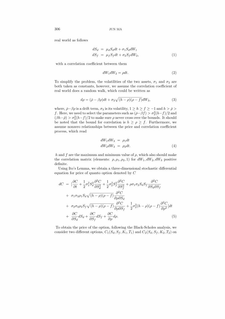
is the initial correlation at time t = 0. It could be found the difference issmall since the diffusion at T = 0.15 results in a weak deviation of ρ fromthe initial value ρ0. Taking parameters same as in Fig.1 except T = 0.30,we compare the results with the price for constant coefficient in Fig.2, andcould find larger price difference than in Fig. 1. But we should note that(C

′(ρ0)−C(ρ0))/Kf for this option is large only around ρ ∼ ±0.9 in Figs.

1 and 2. We note that the larger Sf (t = 0), the bigger difference betweenC

′(ρ0)−C(ρ0), which is exactly why we choose fixed exchange rate foreign

equity call as example. In fact, other kinds of foreign equity option such asforeign equity call struck in foreign currency, and foreign call in domesticcurrency do not display such a phenomenon. In other words, their pricedifference due to correlation risk is almost zero and independent of ρ0 asSf (t) >> Kf or Sf (t) << Kf . We will elucidate why in the next section.

3. THE STANDARD JACOBI DIFFERENTIAL EQUATION

It is known that the stochastic volatility is important as well as the cor-relation risk and they might have same source. For example, a firm’s valuecan be decomposed as the net present value of all its forthcoming incomewith its asset minus its debt. Their components have different volatilitieswhich cause the leverage related skew of the implied volatility. On the otherhand, economic effects, e.g., anticipated central bank action, give rise to aninterest rate skew of volatility, which is elucidated by the stochastic volatil-ity. Then the same question arises for correlation coefficients. It is obviousthat the correlation coefficients between those pairs of component in a firm’svalue must differ each other, which attributes to the stochastic correlation.The only difference between two cases is: to calibrate the market data ofthe skew or smile, we need to set up a comparatively strong correlationbetween the stochastic process of volatility and the one of equity. But,the correlation process could be independent or weakly connected to the

310 JUN MA

FIG. 1. The price differenceC′(ρ0)−C(ρ0)

Kffor T = 0.15. C

′(ρ0) stands for the price

of quanto option with the stochastic correlation coefficient, and C(ρ0) is the one with

constant correlation coefficient, and Kf is the strike price. The parameters for C′

aretaken as S̄d = 1, rf = 0.1 σ1 = 1.0, σ2 = 1.0, T = 0.15, ρ̄ = −0.01, ρ1 = −ρ2 = 0.01,g = 2.0, σ3 = 1.0 and h = 0.9, f = −0.9. All parameters are same except the constantcorrelation is taken as ρ0 for C where ρ0 is the correlation of the initial time.

one of equity. Since generally, the empirical evidence shows that randomcorrelation could move from 1 to -0.5 or even to -1 which suppresses ρ1 andρ2 to make the correlation matrix positive definite, i.e., ρ1 ≈ 0 and ρ2 ≈ 0(see Eq.(9)), we could use the pricing formula derived in this section forρ1 = ρ2 = 0 with confidence.

Notice that we have not even introduced so far what stochastic volatilitycould be incorporated in this model. Certainly, we could generalize themodel in Sec.2 to include the effect of stochastic volatilities of securities aswell. Heston has considered the following process to describe the randomwalk of volatility (see Heston, 1993) dPk = (ek − akPk)dt + γkP

αk

k dVk

where Pk = σ2k, ek and ak are two positive parameters, γk represents the

amplitude of change of volatility, αk stands for a positive parameter lessthan 1, and dVk is a standard Weiner process. Furthermore, we could usedρj = (ρ̄j − gjρj)dt−

√(hj − ρj)(ρj − fj)dWj to describe correlations in a

set of underlying asset Sk where 1 ≤ k ≤ N , and 1 ≤ j ≤ N(N−1)/2. Theneach pair of processes contributes a correlation coefficient as an element ofthe correlation matrix. It is very difficult to figure out a formula like


FIG. 2. The price differenceC′(ρ0)−C(ρ0)

Kffor T = 0.30. All parameters are same

as in the figure 1 except T = 0.30.

Eq.(9) to guarantee this correlation matrix is positive definite. But a non-zero measure must exist for such a set of process since at least we couldset each process as independent one even if highlighting the stochasticvolatilities. Then, we could use the Heston process and the modified orstandard Jacobi process to describe the random walks of volatility andcorrelation in N -dimensional assets, which could make the pricing modelmore sophisticated.

Generally, we should look for a closed form solution because of its con-venience in practice. Regardless of that the closed form solution for thiskind of stochastic process is currently unavailable, when choosing somespecial parameters, an approximate formula still could be derived. In lastsection, we recommend the Jacobi processes to describe the risk-neutralmotion of correlation, i.e., dρ = (ρ̄− gρ)dt + σ3

√(h− ρ)(ρ− f)dW3. To

simplify the problem, we select ρ1 = ρ2 = 0 to keep the correlation matrixdefinite positive. Now, the motion of correlation and the one of asset priceare independent, then, using the Kolmogorov forward equation, we couldsolve the probability kernel for the correlation process easily. Therefore,the problem is how to determine the eigenvalue λn and eigenfunction ψn(ρ)

312 JUN MA

of the Markov generator of the process, which is

H =σ2

3

2(h− ρ)(ρ− g)

d2

dρ2+ (ρ̄− gρ)

d

dρ. (14)

The eigenfunctions of operator H solve the equation

Hψn(ρ) = λnψn(ρ), (15)

which could be solved by variable separation method as follows

σ23

2(h− ρ)(ρ− f)

d2ψn(ρ)dρ2

+ (ρ̄− gρ)dψn(ρ)dρ

+ λnψn(ρ) = 0. (16)

Introducing a transformation like ρ = h−f2 ρ

′+ h+f

2 , we rewrite the Eq.(16)as

σ23

2(1−ρ

′2)d2ψn(ρ

′)

dρ′2 +(

2ρ̄h− f

−gh+ f

h− f−gρ

′)dψn(ρ

′)

dρ′+λnψn(ρ

′) = 0. (17)

Then multiplying 2σ23

in both sides, we get a standard Jacobi differentialequation (see Szego, 1975)

(1−ρ′2

)d2ψn(ρ

′)

dρ′2 +

[2σ2

3

(2ρ̄− hg − fg

h− f)− 2

σ23

gρ′]dψn(ρ

′)

dρ′+

2σ2

3

λnψn(ρ′) = 0,

(18)whose solutions yield

λn = −σ23

2n(n+

2gσ2

3

− 1) (19)

and

ψn(ρ′) =

(2n+ 2gσ23− 1)Γ(n+ 2g

σ23− 1)n!

22g

σ23−1

Γ(n+ 2gh−2ρ̄σ23(h−f)

)Γ(n+ 2ρ̄−2gfσ23(h−f)

)

1/2

P( 2gh−2ρ̄

σ23(h−f)

−1, 2ρ̄−2gf

σ23(h−f)

−1)

n (ρ′).

(20)The Jacobi polynomials are as the following

P( 2gh−2ρ̄

σ23(h−f)

−1, 2ρ̄−2gf

σ23(h−f)

−1)

n (ρ′)

=( 2gh−2ρ̄

σ23(h−f)

)n

n! 2F1

(−n, n+

2gσ2

3

− 1;2gh− 2ρ̄σ2

3(h− f);1− 2ρ

h−f + h+fh−f

2

),(21)


where ( 2gh−2ρ̄σ23(h−f)

)n = ( 2gh−2ρ̄σ23(h−f)

)( 2gh−2ρ̄σ23(h−f)

+ 1)( 2gh−2ρ̄σ23(h−f)

+ 2) · · · ( 2gh−2ρ̄σ23(h−f)

+ n)and 2F1 is the hypergeometric polynomials. Basing on (gh− ρ̄) > σ2

3(h−f)/2 and 0 < h − f ≤ 2, we know (2gh−2ρ̄)

σ23(h−f)

> 0. Then the probabilitykernel for the Jacobi process, P (ρ0, ρ; t, T ) could be written as

P (ρ0, ρ; 0, τ) = (22)∞X

n=0

eλnτ (1 +h+ f

h− f−

2ρ

h− f)

2gh−2ρ̄

σ23(h−f)

−1(1 −

h+ f

h− f+

2ρ

h− f)

2ρ̄−2gf

σ23(h−f)

−1ψn(ρ0)ψn(ρ),

where τ = T − t.The probability kernel of whole system might be impossibly available,

which raises difficulty to get the closed form solution. However, we stillcould derive a solution of a Taylor series expansion. First, we know the priceof the option with two assets S1 and S2 at maturity T is determined by theterminal distribution of its payoff, which is denoted as PO[S1(T ), S2(T )].Then the option price at t yields

C(S1(t), S2(t), ρt, t) =

e−r(T−t)

Z ∞0

Z ∞0

PO[S1(T ), S2(T )]ω[S1(T ), S2(T )|S1(t), S2(t), ρt]dS1(T )dS2(T ),

(23)

where ω[S1(T ), S2(T )|S1(t), S2(t), ρt] is the conditional probability densityfunction of S1(T ), S2(T ) in the risk-neutral world given S1(t), S2(t) and ρt.Second, since the option price is determined by the terminal distributionof price process of the underlying asset instantaneously uncorrelated withthe Jacobi process, we could define another independent variable, i.e., theaveraged correlation coefficient during the life of the option,

ρ̂ =1τ

∫ τ

0

ρtdt, (24)

to solve the conditional probability density function in Eq.(23). Always,we could equally divide a ρ̂ path into k pieces from 0 to τ , and eachtime piece is ∆t. Consequently, it could be defined that Si

1, Si2 are as-

set price at the end of the ith period and their correlation is ρi−1. Then[ln(Si

1/Si−11 ), ln(Si

2/Si−12 )] yield a multi-variate normal distribution. It is

known that S1, S2 are instantaneously uncorrelated with the correlationprocess, which means the probability distribution of [ln(Si

1/Si−11 ), ln(Si

2/Si−12 )]

is conditioned on ρi−1. Basing on the Cholesky decomposition, we useσ1∆W i

1 and σ2(ρi∆W i1+√

1− ρ2i ∆W2) to describe [ln(Si+1

1 /Si1), ln(Si+1

2 /Si2)].

It could be justified that covariance between ln(Si+11 /Si

1)+ln(Si1/S

i−11 ) and

ln(Si+12 /Si

2) + ln(Si2/S

i−12 ) is σ1σ2(ρi + ρi−1)∆t, the variance of asset one

is 2σ21∆t, and the one of asset two is σ2

2(ρ2i +1− ρ2

i + ρ2i−1 +1− ρ2

i−1)∆t =2σ2

2∆t, which indicate the distribution of [ln(Si+11 /Si−1

1 ), ln(Si+12 /Si−1

2 )] is

314 JUN MA

normal with the correlation ρi+ρi−12 . Hence, the probability distribution

of [ln(Sk1 /S

01), ln(Sk

2 /S02)] conditioned on the path follow by ρ is normal

with a correlation ρ̂, which depends on ρ̂ only. On the other hand, if thestochastic dynamic generates an infinite number of paths that give the sameaveraged correlation ρ̂, they must generate a same terminal distribution ofasset price. Thus, using the formula for the conditional density functionwith several random variables, the conditional probability density functionof terminal asset prices could be rewritten as

ω[S1(T ), S2(T )|S1(t), S2(t), ρt)]

=∫ h

f

Λ[S1(T ), S2(T )|S1(t), S2(t), ρ̂]ε[ρ̂|S1(t), S2(t), ρt]dρ̂, (25)

where Λ[S1(T ), S2(T )|S1(t), S2(t), ρ̂] means the class of path of S1, S2 con-ditional upon ρ̂. Substituting the above equation into Eq.(23), the optionprices turns to be

C(S1(t), S2(t), ρt, t)

= e−r(T−t)

∫ ∞0

∫ ∞0

∫ h

f

PO[S1(T ), S2(T )]Λ[S1(T ), S2(T )|S1(t), S2(t), ρ̂]

× ε[ρ̂|S1(t), S2(t), ρt]dρ̂dS1(T )dS2(T )

=∫ h

f

{e−r(T−t)

∫ ∞0

∫ ∞0

PO[S1(T ), S2(T )]Λ(S1(T ), S2(T )|S1(t), S2(t), ρ̂)

× dS1(T )dS2(T )}ε[ρ̂|S1(t), S2(t), ρt]dρ̂. (26)

As mentioned before, the prices of the underlying asset follow geometricBrownian motions, which guarantees the class of path of S1, S2 conditionalupon ρ̂, i.e., Λ[S1(T ), S2(T )|S1(t), S2(t), ρ̂], generates a standard lognormaldistribution. Then in above equation, the inner integral produces nothingbut the Black-Scholes formula with a varying correlation coefficient: theconstant correlation coefficient is replaced by ρ̂. Finally, the option valueyields

C(S1, S2, ρt) =∫ h

f

CBS(ρ̂)ε(ρ̂)dρ̂, (27)

where CBS stands for the Black-Scholes pricing formula with correlation ρ̂.Although it is difficult to derive ε(ρ̂), remembering the kernel of the Jacobiprocess is available, nevertheless, we could obtain the moments of ρ̂ andsubstitute them to expand the above formula. Consequently, the option


pricing formula could be written in its Taylor series as follows

C(S1(t), S2(t), ρt)

= CBS(ρ̂) +1

2

∂2CBS

∂ρ2|ρ̂Var(ρ̂) +

1

6

∂3CBS

∂ρ3|ρ̂Skew(ρ̂) + · · ·

= CBS(ρ̂) +1

2

∂2CBS

∂ρ2|ρ̂(ρ̂2 − (ρ̂)2) +

1

6

∂3CBS

∂ρ3|ρ̂(ρ̂3 − 3ρ̂2 · ρ̂ + 2(ρ̂)3) + · · · .

(28)

Now, the unsolved problem is to evaluate ρ̂, ρ̂2, ρ̂3, and so on. Using theevolution kernel of the risk-neutral Jacobi process P (ρ0, ρ; 0, t) to derivethe expectation of ρ̂, i.e., EQ( 1

τ

∫ τ

0ρtdt), it is easy to get ρ̂, which reads

ρ̂ =1τ

∫ h

f

∫ τ

0

ρP (ρ0, ρ; 0, t)dtdρ

=1τ

∫ h

f

∫ τ

0

[ρ∞∑

n=0

e−σ2

32 n(n+ 2g

σ23−1)τ

(1 +h+ f

h− f− 2ρh− f

)2gh−2ρ̄

σ23(h−f)

−1

×(1− h+ f

h− f+

2ρh− f

)2ρ̄−2gf

σ23(h−f)

−1ψn(ρ0)ψn(ρ)]dtdρ

=∞∑

n=0

1− e−σ2

32 n(n+ 2g

σ23−1)τ

σ232 n(n+ 2g

σ23− 1)τ

ψn(ρ0)∫ h

f

dρ[ρ(1 +h+ f

h− f− 2ρh− f

)2gh−2ρ̄

σ23(h−f)

−1

×(1− h+ f

h− f+

2ρh− f

)2ρ̄−2gf

σ23(h−f)

−1ψn(ρ)]. (29)

It is a little tricky to derive ρ̂2. First, we rewrite the expectation of ρ̂2 as1τ2E

Q[(∫ τ

0ρt1dt1)(

∫ τ

0ρt2dt2)] = 1

τ2EQ[∫ τ

0

∫ τ

0ρt1ρt2dt1dt2], and divide the

integrating domain into two parts, i.e., part t1 > t2 and the other t2 > t1,whose contributions to the final value are same. Second, selecting one part,and substituting

EQ[

Z τ

0

Z τ

0ρt1ρt2dt1dt2]

=2

τ2

Z τ

0dt1

Z h

fdρxρxP (ρ0, ρx; 0, t1)

Z τ−t1

0dt2

Z h

fdρyρyP (ρx, ρy ; 0, t2), (30)

316 JUN MA

we get

ρ̂2 =2

τ2

Z h

f{

Z τ

0[ρxP (ρ0, ρx; 0, t1)

Z h

fρy

Z τ−t1

0P (ρx, ρy ; 0, t2)dt2dρy ]dt1}dρx

=2

τ2

∞Xn,m=0

[1 − e

−σ232 n(n+ 2g

σ23−1)τ

σ434m(m+ 2g

σ23− 1)n(n+ 2g

σ23− 1)

−e−

σ232 m(m+ 2g

σ23−1)τ

− e−

σ232 n(n+ 2g

σ23−1)τ

σ434m(m+ 2g

σ23− 1)(n(n+ 2g

σ23− 1) −m(m+ 2g

σ23− 1))

]

× ψn(ρ0)

Z h

f

Z h

fdρxdρy [ρx(1 +

h+ f

h− f−

2ρx

h− f)

2gh−2ρ̄

σ23(h−f)

−1

× (1 −h+ f

h− f+

2ρx

h− f)

2ρ̄−2gf

σ23(h−f)

−1ψn(ρx)ψm(ρx)ρy(1 +

h+ f

h− f−

2ρy

h− f)

2gh−2ρ̄

σ23(h−f)

−1

× (1 −h+ f

h− f+

2ρy

h− f)

2ρ̄−2gf

σ23(h−f)

−1ψm(ρy)]. (31)

At last, following the same algorithms, we rewrite the expectation of ρ̂3 as1τ3E

Q[∫ τ

0

∫ τ

0

∫ τ

0ρt1ρt2ρt3dt1dt2dt3] and divide the integrating domain into

six parts, i.e., t3 > t2 > t1, t3 > t1 > t2, t2 > t1 > t3, t2 > t3 > t1,t1 > t3 > t2, t1 > t2 > t3, whose contributions to total value are same.Then, performing the following integration

EQ[∫ τ

0

∫ τ

0

∫ τ

0

ρt1ρt2ρt3dt1dt2dt3]

=6τ3

∫ h

f

dρx

∫ τ

0

dt1ρxP (ρ0, ρx; 0, t1)∫ h

f

dρy

∫ τ−t1

0

dt2ρyP (ρx, ρy; 0, t2)

×∫ h

f

dρz

∫ τ−t2−t1

0

dt3ρzP (ρy, ρz; 0, t3), (32)


and substituting it, we get

ρ̂3

=6

τ3

∞Xn=0

m=0,l=0

[e−

σ232 m(m+ 2g

σ23−1)τ

− e−

σ232 n(n+ 2g

σ23−1)τ

σ638l(l + 2g

σ23− 1)(m(m+ 2g

σ23− 1) − l(l + 2g

σ23− 1))(n(n+ 2g

σ23− 1) −m(m+ 2g

σ23− 1))

−e−

σ232 l(l+ 2g

σ23−1)τ

− e−

σ232 n(n+ 2g

σ23−1)τ

σ638l(l + 2g

σ23− 1)(m(m+ 2g

σ23− 1) − l(l + 2g

σ23− 1))(n(n+ 2g

σ23− 1) − l(l + 2g

σ23− 1))

−e−

σ232 m(m+ 2g

σ23−1)τ

− e−

σ232 n(n+ 2g

σ23−1)τ

σ638l(l + 2g

σ23− 1)m(m+ 2g

σ23− 1)(n(n+ 2g

σ23− 1) −m(m+ 2g

σ23− 1))

+1 − e

−σ232 n(n+ 2g

σ23−1)τ

σ638l(l + 2g

σ23− 1)m(m+ 2g

σ23− 1)n(n+ 2g

σ23− 1)

]ψn(ρ0)

×Z h

f

Z h

f

Z h

fdρxdρydρz [ρx(1 +

h+ f

h− f−

2ρx

h− f)

2gh−2ρ̄

σ23(h−f)

−1

× (1 −h+ f

h− f+

2ρx

h− f)

2ρ̄−2gf

σ23(h−f)

−1ψn(ρx)ψm(ρx)

× ρy(1 +h+ f

h− f−

2ρy

h− f)

2gh−2ρ̄

σ23(h−f)

−1(1 −

h+ f

h− f+

2ρy

h− f)

2ρ̄−2gf

σ23(h−f)

−1ψm(ρy)ψl(ρy)

× ρz(1 +h+ f

h− f−

2ρz

h− f)

2gh−2ρ̄

σ23(h−f)

−1(1 −

h+ f

h− f+

2ρz

h− f)

2ρ̄−2gf

σ23(h−f)

−1ψl(ρz)]. (33)

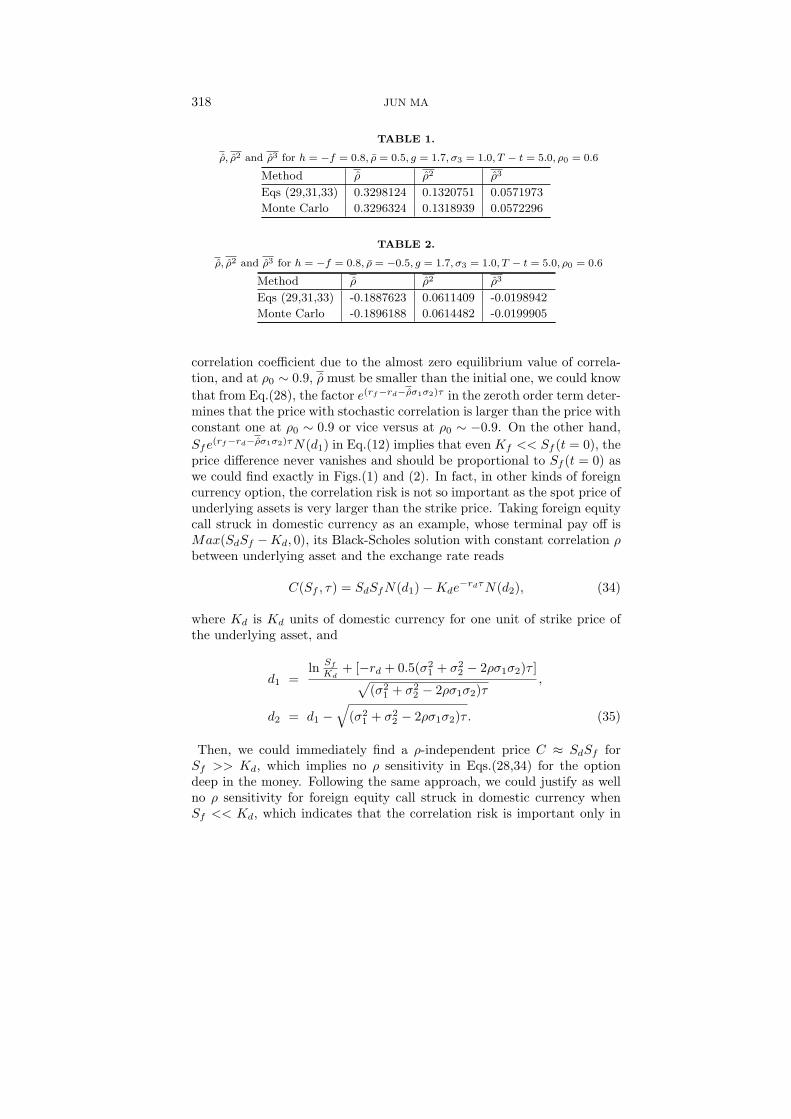
Basing on the fact that the kurtosis of ρ̂ is generally much less than0.001 because of |ρt| ≤ 1, absolute value of the fourth term in Eq.(28)is basically much less than one basis point. Thus, it is not necessary toderive ρ̂4 and even higher order terms. We testify Eqs.(29,31,33) and com-pare the computation result with the one from the Monte Carlo methodin Tables 1 and 2. Remembering that this Monte Carlo simulation is justone-dimensional and should have high accuracy, it is not surprising to ob-serve that the numerical outcomes from two methods in Tables 1 and 2 arealmost same. We need to point out that in Eqs.(29,31,33), the first coupleof eigenvalue and eigenfunctions generally could guarantee very good accu-racy since the eigenvalue λn ∼ −n2 and the exponentially decaying factoreλnτ suppresses most of terms in Eqs.(29,31,33). Moreover, the first innerintegration in Eqs.(29,31,33) could be performed analytically, which makesthese equations more efficient.

An important subject is to analyze the numerical option price withinthe framework of Eq.(28). Substituting Black-Scholes solution of quantooption into Eq.(28), immediately, we could understand what happens inFigs. (1) and (2). Since at ρ0 ∼ −0.9, ρ̂ must be larger than the initial

318 JUN MA

TABLE 1.

ρ̂, ρ̂2 and ρ̂3 for h = −f = 0.8, ρ̄ = 0.5, g = 1.7, σ3 = 1.0, T − t = 5.0, ρ0 = 0.6

Method ρ̂ ρ̂2 ρ̂3

Eqs (29,31,33) 0.3298124 0.1320751 0.0571973

Monte Carlo 0.3296324 0.1318939 0.0572296

TABLE 2.

ρ̂, ρ̂2 and ρ̂3 for h = −f = 0.8, ρ̄ = −0.5, g = 1.7, σ3 = 1.0, T − t = 5.0, ρ0 = 0.6

Method ρ̂ ρ̂2 ρ̂3

Eqs (29,31,33) -0.1887623 0.0611409 -0.0198942

Monte Carlo -0.1896188 0.0614482 -0.0199905

correlation coefficient due to the almost zero equilibrium value of correla-tion, and at ρ0 ∼ 0.9, ρ̂ must be smaller than the initial one, we could knowthat from Eq.(28), the factor e(rf−rd−ρ̂σ1σ2)τ in the zeroth order term deter-mines that the price with stochastic correlation is larger than the price withconstant one at ρ0 ∼ 0.9 or vice versus at ρ0 ∼ −0.9. On the other hand,Sfe

(rf−rd−ρ̂σ1σ2)τN(d1) in Eq.(12) implies that even Kf << Sf (t = 0), theprice difference never vanishes and should be proportional to Sf (t = 0) aswe could find exactly in Figs.(1) and (2). In fact, in other kinds of foreigncurrency option, the correlation risk is not so important as the spot price ofunderlying assets is very larger than the strike price. Taking foreign equitycall struck in domestic currency as an example, whose terminal pay off isMax(SdSf −Kd, 0), its Black-Scholes solution with constant correlation ρbetween underlying asset and the exchange rate reads

C(Sf , τ) = SdSfN(d1)−Kde−rdτN(d2), (34)

where Kd is Kd units of domestic currency for one unit of strike price ofthe underlying asset, and

d1 =ln Sf

Kd+ [−rd + 0.5(σ2

1 + σ22 − 2ρσ1σ2)τ ]√

(σ21 + σ2

2 − 2ρσ1σ2)τ,

d2 = d1 −√

(σ21 + σ2

2 − 2ρσ1σ2)τ . (35)

Then, we could immediately find a ρ-independent price C ≈ SdSf forSf >> Kd, which implies no ρ sensitivity in Eqs.(28,34) for the optiondeep in the money. Following the same approach, we could justify as wellno ρ sensitivity for foreign equity call struck in domestic currency whenSf << Kd, which indicates that the correlation risk is important only in


Sf ∼ Kd region. Then one could understand why we choose quanto optionas an example to illustrate the price difference which is proportional to thevalue of underlying asset.

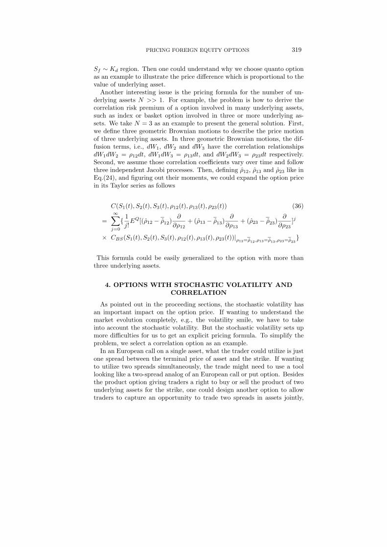
Another interesting issue is the pricing formula for the number of un-derlying assets N >> 1. For example, the problem is how to derive thecorrelation risk premium of a option involved in many underlying assets,such as index or basket option involved in three or more underlying as-sets. We take N = 3 as an example to present the general solution. First,we define three geometric Brownian motions to describe the price motionof three underlying assets. In three geometric Brownian motions, the dif-fusion terms, i.e., dW1, dW2 and dW3 have the correlation relationshipsdW1dW2 = ρ12dt, dW1dW3 = ρ13dt, and dW2dW3 = ρ23dt respectively.Second, we assume those correlation coefficients vary over time and followthree independent Jacobi processes. Then, defining ρ̂12, ρ̂13 and ρ̂23 like inEq.(24), and figuring out their moments, we could expand the option pricein its Taylor series as follows

C(S1(t), S2(t), S3(t), ρ12(t), ρ13(t), ρ23(t)) (36)

=∞∑

j=0

{ 1j!EQ[(ρ̂12 − ρ̂12)

∂

∂ρ12+ (ρ̂13 − ρ̂13)

∂

∂ρ13+ (ρ̂23 − ρ̂23)

∂

∂ρ23]j

× CBS(S1(t), S2(t), S3(t), ρ12(t), ρ13(t), ρ23(t))|ρ12=ρ̂12,ρ13=ρ̂13,ρ23=ρ̂23}

This formula could be easily generalized to the option with more thanthree underlying assets.

4. OPTIONS WITH STOCHASTIC VOLATILITY ANDCORRELATION

As pointed out in the proceeding sections, the stochastic volatility hasan important impact on the option price. If wanting to understand themarket evolution completely, e.g., the volatility smile, we have to takeinto account the stochastic volatility. But the stochastic volatility sets upmore difficulties for us to get an explicit pricing formula. To simplify theproblem, we select a correlation option as an example.

In an European call on a single asset, what the trader could utilize is justone spread between the terminal price of asset and the strike. If wantingto utilize two spreads simultaneously, the trade might need to use a toollooking like a two-spread analog of an European call or put option. Besidesthe product option giving traders a right to buy or sell the product of twounderlying assets for the strike, one could design another option to allowtraders to capture an opportunity to trade two spreads in assets jointly,

320 JUN MA

whose payoff is Max[S1(T )−K1, 0]×Max[S2(T )−K2, 0] (see Bakishi andMadan, 2000).

Selecting this kind of option as an example, we could investigate an im-portant issue, i.e., pricing option with stochastic volatility and correlation.First, we suppose the trader could use the correlation option to bet thespreads in the foreign exchange rate or asset. Second, no foreign exchangerate or asset keeps constant volatility, and all stochastic volatilities shareone random source. Consequently, the dynamics with stochastic volatilitycould be selected as follows (see Jegadeesh and Tuckman, 2000; Bakishiand Madan, 2000)

dS1

S1= (rd − rf )dt+ σ1

√QdW1,

dS2

S2= (rd − rf )dt+ σ2

√QdW2,

dQ = (θq − kqQ)dt+ σq

√QdWq, (37)

where Q represents a volatility factor, rd, rf are domestic and foreigninterest rate respectively, we specify dW1dW2 = ρdt, dW1dWq = ρ̄1dt, anddW2dWq = ρ̄2dt. This ρ-constant dynamics values the correlation optionC(S1, S2, Q0, τ) as

C(S1, S2, Q0, τ) = (38)

e−ζ1 ln K1−ζ2 ln K2

(2π)2

Z ∞−∞

Z ∞−∞

Re[e−i(φ1 ln K1+φ2 ln K2)−rdτG(τ ;χ1, χ2)

(ζ1 + iφ1)(ζ1 + 1 + iφ1)(ζ2 + iφ2)(ζ2 + 1 + iφ2)]dφ2dφ1,

where Q0 is initial volatility, ζ1 and ζ2 are chosen as two real numbersto define χ1 = φ1 − (1 + ζ1)i, χ2 = φ2 − (1 + ζ2)i, and the characteristicfunction is

G(τ ;χ1, χ2) = exp[iχ1 lnS1(0) + iχ2 lnS2(0) + i(χ1 + χ2)(rd − rf )τ

+2η(1− e−θτ )

2θ − (θ − ϕ)(1− e−θτ )Q0

− 2θq

σ2q

ln(1− (θ − ϕ)(1− e−θτ )2θ

)− θq

σ2q

(θ − ϕ)τ ], (39)

with

ϕ = kq − i(ρ̄1σ1χ1 + ρ̄2σ2χ2)σq

θ =√ϕ2 − 2σ2

qη

η = −0.5(σ21χ

21 + σ2

2χ22 + 2ρσ1σ2χ1χ2)− 0.5i(σ2

1χ1 + σ22χ2). (40)


Having defined an independent Jacobi process to describe the randommotion of correlation ρ, we could use Eq.(28) to derive the price of the op-tion with stochastic volatility and correlation. Furthermore, the sensitivityof option price versus the correlation is

∂G

∂ρ= (−2

θqX2

σ2qX1

+θqτX0

θ+Q0

X4

X23

)G (41)

with

X0 = −σ1σ2χ1χ2

y0 = −σ2qX0(1− e−θτ )/θ − (θ − ϕ)τσ2

qX0e−θτ/θ

X1 = 1− (θ − ϕ)(1− e−θτ )2θ

X2 = −0.5σ2

qX0(θ − ϕ)(1− e−θτ )θ3

− 0.5y0θ

X3 = 2θ − (θ − ϕ)(1− e−θτ )X4 = 2X0(1− e−θτ )X3 − 2ητσ2

qX0X3e−θτ/θ

+ 2η(1− e−θτ )(2σ2qX0/θ + y0). (42)

The second order is

∂2G

∂ρ2= [−2θq(X5X1 −X2

2 )/(σ2qX

21 ) + θqσ

2qτX

20/θ

3 +X6Q0/X23

+ 4σ2qX0X4Q0/(X3

3θ) + 2X4y0Q0/X33 ]G

+ (−2θqX2/(σ2qX1) + θqτX0/θ +X4Q0/X

23 )∂G

∂ρ(43)

with

X5 = −σ2qX0y0/θ

3 − 0.5y1/θ −32σ4

qX20 (θ − ϕ)(1− e−θτ )/θ5

X6 = −2X20X3τσ

2qe−θτ/θ − 2X0(1− e−θτ )(2σ2

qX0/θ + y0)

− 2τσ2qX

20X3e

−θτ/θ + 2ητσ2qX0e

−θτ (2σ2qX0/θ + y0)/θ

− 2ητ2σ4qX

20X3e

−θτ/θ2 − 2ητσ4qX

20X3e

−θτ/θ3

+ 2X0(1− e−θτ )(2σ2qX0/θ + y0) + 2ηX7

X7 = −2τσ4qX

20e−θτ/θ2 − τσ2

qX0y0e−θ1τ/θ + (1− e−θτ )(2σ4

qX20/θ

3 + y1)

y1 = τσ4qX

20e−θτ/θ2 − σ4

qX20 (1− e−θτ )/θ3 + τσ4

qX20e−θτ/θ2

− (θ − ϕ)τ2σ4qX

20e−θτ/θ2 − (θ − ϕ)τσ4

qX20e−θτ/θ3. (44)

322 JUN MA

The third order is

∂3G

∂ρ3= [−2θqX8/(σ2

qX1) + 2θqX5X2/(σ2qX

21 ) + 4θqX2X5/(σ2

qX21 )

− 4θqX32/(σ

2qX

31 ) + 3θqτσ

4qX

30/θ

5

+ X9Q0/X23 + 2X6(2σ2

qX0/θ + y0)Q0/X33 + 4σ2

qX0X6Q0/(X23θ)

+ 12σ2qX0X4(2σ2

qX0/θ + y0)Q0/(X43θ) + 4σ4

qX20X4Q0/(X3

3θ3)

+ 2X6y0Q0/X33 + 2X4y1Q0/X

33 + 6X4y0(2σ2

qX0/θ + y0)Q0/X43 ]G

+ 2[−2θqX5/(σ2qX1) + 2θqX

22/(σ

2qX

21 ) + θqτσ

2qX

20/θ

3

+ X6Q0/X23 + 4σ2

qX0X4Q0/(X33θ) + 2X4y0Q0/X

33 ]∂G

∂ρ

+ [−2θqX2/(σ2qX1) + θqτX0/θ +X4Q0/X

23 ]∂2G

∂ρ2(45)

with

X8 = −y1σ2qX0/θ

3 − 92y0σ

4qX

20/θ

5 − 12y2/θ −

12σ2

qX0y1/θ3

− 152σ6

qX30 (θ − ϕ)(1− e−θτ )/θ7

X9 = 6τσ2qX

20 (2σ2

qX0/θ + y0)e−θτ/θ − 6τ2σ4qX

30X3e

−θτ/θ2

− 6τσ4qX

30X3e

−θτ/θ3 + 4ητ2σ4qX

20e−θτ (2σ2

qX0/θ + y0)/θ2

+ 2ητσ2qX0e

−θτ (2σ4qX

20/θ

3 + y1)/θ + 4ητσ4qX

20e−θτ (2σ2

qX0/θ + y0)/θ3

− 2ητ3σ6qX

30e−θτ/θ3 − 6ητ2σ6

qX30e−θτX3/θ

4

− 6ητσ6qX

30e−θτX3/θ

5 + 2x0X7 + 2ηX10

X10 = −2τ2σ6qX

30e−θτ/θ3 − 4τσ6

qX30e−θτ/θ4 − τσ2

qX0y1e−θτ/θ

− τ2σ4qX

20y0e

−θτ/θ2 − τσ4qX

20y0e

−θτ/θ3

− τσ2qX0(2σ4

qX20/θ

3 + y1)e−θτ/θ + (1− e−θτ )(6σ6qX

30/θ

5 + y2)

y2 = 3τ2σ6qX

30e−θτ/θ3 + 6τσ6

qX30e−θτ/θ4

− 3σ6qX

30 (1− e−θτ )/θ5 − (θ − ϕ)τ3σ6

qX30e−θτ/θ3

− 3(θ − ϕ)τ2σ6qX

30e−θτ/θ4 − 3(θ − ϕ)τσ6

qX30e−θτ/θ5. (46)

Substituting ∂G∂ρ ,

∂2G∂ρ2 , and ∂3G

∂ρ3 , and utilizing the algorithm introduced inSec. 3 and Eqs.(29,31,33) for ρ̂, ρ̂2, ρ̂3, we could arrive at the final formula


for pricing the option with stochastic volatility and correlationC(S1, S2, Q0, ρ0)

=e−ζ1 ln K1−ζ2 ln K2

(2π)2

Z ∞−∞

Z ∞−∞

Re[e−i(φ1 ln K1+φ2 ln K2−irdτ)G(τ ;χ1, χ2)

(ζ1 + iφ1)(ζ1 + 1 + iφ1)(ζ2 + iφ2)(ζ2 + 1 + iφ2)]dφ2dφ1

+1

2


(2π)2

Z ∞−∞

Z ∞−∞

Re[e−i(φ1 ln K1+φ2 ln K2−irdτ) ∂2G(τ ;χ1,χ2)

∂ρ2 |ρ̂(ζ1 + iφ1)(ζ1 + 1 + iφ1)(ζ2 + iφ2)(ζ2 + 1 + iφ2)

]dφ2dφ1

× (ρ̂2 − (ρ̂)2)

+1

6


(2π)2

Z ∞−∞

Z ∞−∞

Re[e−i(φ1 ln K1+φ2 ln K2−irdτ) ∂3G(τ ;χ1,χ2)

∂ρ3 |ρ̂(ζ1 + iφ1)(ζ1 + 1 + iφ1)(ζ2 + iφ2)(ζ2 + 1 + iφ2)

]dφ2dφ1

× (ρ̂3 − 3ρ̂2 · ρ̂+ 2(ρ̂)3) + · · · . (47)

Although the above formula is just for two-asset option, in fact, substi-tuting a stochastic volatility pricing formula of index or basket option intoEq.(36), we could get the volatility and correlation risk pricing formulainvolving three or more underlying assets.

Before testifying the numerical method, in Eq.(37) model, we always cannormalize the terminal payoff of the correlation as K1K2Max[S1(T )

K1− 1]×

Max[S2(T )K2

− 1]. Then taking K1 = K2 = 1 is convenient, which does notlose any generality at all. We use the Monte Carlo method and Eq.(38)to compute the price of Eq.(37) model with constant ρ. In Sec. 3, wefind the numerical outcome from one-dimensional Monte Carlo matchesEqs.(29,31,33) well. But to compute Eq.(37) with constant ρ, the MonteCarlo must be multi-dimensional, which unfortunately lessens its accuracy.In lines (1) and (2) of Fig.3, taking K1 = K2 = 1, S1(0) = 1.1, S2(0) = 1.2τ = 5, rd = 0.1, rf = 0.05, ρ = 0.6, ρ̄1 = ρ̄2 = −0.2, Q0 = 0.8 σ1 = 0.5,σ2 = 0.6, θq = 0.5, κq = 1.0, and σq = 0.5, the semi-closed form solution,Eq.(38) for constant ρ = 0.6 gives the price 0.905, but the asymptotic pricefor constant ρ = 0.6 from the Monte Carlo method is 0.899. Taking sameparameters of lines (1) and (2) except ρ, we also computed the price forconstant ρ = −0.6, and found the comparatively large fluctuation in theMonte Carlo method. Finally, we take 0.455 as the asymptotic price forρ = −0.6 and get the price 0.468 from Eq.(38), which are not plotted inFig.3. The averaged error for constant ρ is about 0.004. But in negativecorrelation region, since the true option price is comparatively small, theerror of the Monte carlo method looks like a little large. Furthermore, wecompute the option price with stochastic correlation. Since the procedureof proving the series solution Eq.(47) is rigorous and the absolute value ofits fourth term is generally less that one basis point, Eq.(47) highlightingthe first three terms could be treated as a benchmark for other numericalapproaches. As has been expected, one more dimension, i.e., the Jacobi pro-cess, involved in the Monte carlo method, magnifies computational error.The price from the first three terms of Eq.(47) for ρ0 = 0.6, ρ̄ = 0.5 plotted

324 JUN MA

in line (3) is 0.586, but the asymptotic price from the Monte Carlo methodplotted in line (4) is 0.580. Another little bigger difference takes placesin ρ0 = 0.6, ρ̄ = −0.5 case, where line (5) for Eq.(47) gives price 0.188.But in line (6), the Mont Carlo method always presents a comparativelylarge fluctuation, which raise the difficulty to determine the asymptoticprice. Finally, we take 0.196 as its asymptotic value for ρ0 = 0.6, ρ̄ = −0.5,whose relatively large error is due to the negative correlation induced bythe negative equilibrium value during most of the life of the option. In thestochastic correlation cases, it seems that the averaged error of the Montecarlo method is about 0.007, which is almost double of the one in constantcorrelation case. It could be concluded that, using fast Fourier transforma-tion, Eq.(47) is more reliable, efficient and accurate than the Monte carlomethod.

FIG. 3. Lines 1 and 2 give a comparison between the correlation option price ofEq.(37) Model from Eq.(38) with constant correlation and the one from the MonteCarlo method. Lines (1) for Eq.(38) and (2) for the Monte Carlo method share sameparameters, K1 = K2 = 1, S1(0) = 1.1, S2(0) = 1.2, τ = 5, rd = 0.1, rf = 0.05,ρ = 0.6, ρ̄1 = ρ̄2 = −0.2, Q0 = 0.8, σ1 = 0.5, σ2 = 0.6, θq = 0.5, κq = 1.0, andσq = 0.5. Lines (3) and (4) are from Eq.(47) with random correlation and the MonteCarlo method, which share same parameters as in lines (1) and (2) except ρ̄ = 0.5,ρ0 = 0.6, h = −f = 0.8, g = 1.7, σ3 = 1.0. Lines (5) and (6) are from Eq.(47) withrandom correlation and the Monte Carlo method, which share same parameters as inlines (3) and (4) except ρ̄ = −0.5. In this Figure, horizontal coordinate, M , is thenumber of the simulated path, and vertical one is the price of correlation option, C.


5. CONCLUSION

Correlation risk in general sense is generally defined as the differencebetween implied and realized correlation for a given maturity, which canbe frequently found in the market. To derive the pricing formula analyti-cally, we assume the correlation risk premium is linearly proportional to thecurrent level of correlation, which is used to introduce a kind of stochasticprocess, i.e., dρ = (ρ̄−gρ)dt+σ

√(h− ρ)(ρ− f)dW to describe the random

walk of correlation coefficients. In our scheme, the correlation coefficientwanders around the mean value within the region from the upper boundh ≤ 1 to the lower one f ≥ −1. Of course, there are many other waysto define correlation risk premium, and, thus, other risk neutral correla-tion processes are also possible, e.g., dρ = [ρ̄ + g ln

√(h− ρ)(ρ− f)]dt +

σ√

(h− ρ)(ρ− f)dW , which could guarantee the correlation coefficientnever hits the bounds. The pricing equation for stochastic correlation coef-ficient is derived. The obvious difference is numerically found as the quickdiffusion happens in motions of correlation coefficients, which indicates thatwe have to use this model to eliminate correlation risk. At last, we tried tofind whether a series solution for pricing the stochastic volatility and corre-lation simultaneously is available. Supposing that the stochastic process ofcorrelation is independent, we finally developed a series solution for pricingboth of volatility and correlation risks, i.e., Eq.(47) , whose second andthird terms occupy three, five, or ten percents of total value, which couldbe used to capture the feature of structure of implied correlation. Conse-quently, we could use the trading strategy to hedge the correlation risk.For example, if trading a basket option on stocks highlighted in Standardand Poor’s 500, to hedge the correlation risk involved, the trader could ma-nipulate an option on the Standard and Poor index. An alternative way isthat for instance, trading a basket option results in a correlation risk, butit can be hedged by applying a best-of option highlighting the componentof the basket option. Namely, in the currency market, if the correlationrisk results from an option on the basket consisting of U.S. dollar, JapaneseYen, and British pounds, then, a best-of call allows the owner to buy any ofthe currencies that increases the most at the maturity of the option, whichcan be used to hedge the risk.

REFERENCESBall C., and A. Roma, 1994. A Stochastic volatility option pricing. The Journal ofFinancial and Quantitative Analysis 29(4), 589-607.

Bakshi G. and D. Madan, 2000. Spanning and derivative-security valuation. Journalof Financial Economics 55(2), 205-238.

Baz, J. and G. Chacko, 2004. Financial derivatives: pricing, application and mathe-matics. Cambridge University Press.

326 JUN MA

Black F., and M. Scholes, 1973. The Pricing of options and corporate liabilities.Journal of Political Economy. 81(3), 637-654.

Briys E., Bellalah M., Mai H., and F. de Varenne, 1998. Options, futures and exoticderivatives: theory, application and practice. John Wiley & Sons.

Bru M. F. 1991. Wishart Process. Journal of Theoretical Probability 4(4), 725-751.

Buraschi A., Cieslak A., and F. Trojani, 2007. Correlation risk and the term structuresof interest rates. Working paper, Imperial College, London.

Buraschi A., Porchia P., and F. Trojani, 2006. Correlation risk and optimal portfoliochoice. Working paper, Imperial College, London.

Driessen J., Maenhout P., and G. Vilkov, 2006. Option-Implied correlations and theprice of correlation risk. Working paper, INSEAD.

Engle, R., 1982. Autoregressive conditional heteroskedasticity with estimates of thevariance of United Kingdom inflation. Econometrica 50, 987-1008.

Fonseca J., Grasselli M., and C. Tebaldi, 2005. Wishart multi-dimensional stochasticvolatility. Working paper, Ecole Superieure d’Ingenieurs Leonard de Vinci.

Fonseca J., Grasselli M., and C. Tebaldi, 2006. Option pricing when correlations arestochastic: an analytical framework. Working paper, Ecole Superieure d’IngenieursLeonard de Vinci.

Garman M., 1992. Spread the load. Risk 5, 68-84.

Glosten L., Jagannathan R., and D. Runkle, 1993. On the relation between the ex-pected value and the volatility of the nominal excess return on stocks. Journal ofFinance 48(5), 1779-1801.

Gourieroux C., Jasiak J., and R. Sufana, 2004. The wishart autoregressive process ofmultivariate stochastic volatility. Working paper, University of Toronto.

Gourieroux C., and R. Sufana, 2004a. Derivatives pricing with multivariate stochasticvolatility: application to credit risk. Working paper, University of Toronto.

Gourieroux C., and R. Sufana, 2004b. Wishart Quadratic term structure. CREF 03-10, HEC Montreal.

Heston S. L., 1993. A closed-form solution for options with stochastic volatility withapplication to bond and currency options. Review of Financial Studies 6(2), 327-343.

Hull J. C., and A. White, 1987. The Pricing of options on assets with stochasticvolatilities. Journal of Finance 42(2), 281-300.

Hull J. C., and A. White, 1988. An analysis of the Bias in option pricing caused by astochastic volatility. Advances in Advance in Futures and Options Research 3, 27-61.

Jegadeesh N., and B. Tuckman, (eds) 2000. Advanced fixed-income valuation tools.John Wiley & Sons.

Kwok Y. K., 1998. Mathematical models of financial derivatives. Springer Singapore.

Margrable W., 1978. The valuation of an option to exchange one asset for another,Journal of Finance 33, 177-186.

Merton R. C., 1973. The theory of rational option pricing, Bell Journal of Economicsand management science 4(1), 141-183.

Scott L. O., 1987. Option pricing when the variance changes randomly: theory, es-timation and an application, The Journal of Financial and Quantitative Analysis.22(4), 419-438.

Szego G., 1975. Jacobi Polynomials Ch.4 in Orthogonal Polynomials, 4th ed. (Provi-dence, RI: American Mathematical Society).


Taleb N., 1997. Dynamic hedging: managing vanilla and exotic options, John Wiley& Sons.

Zhang P. G., 1998. Exotic options, World Scientific Press.

Pricing Foreign Equity Options with Stochastic Correlation...

Documents

Transcript of Pricing Foreign Equity Options with Stochastic Correlation...