Pricing Financial Derivatives by Gram-Charlier Expansions · 2015-03-02 · RESEARCH PAPER SERIES...

Department of Statistics and Actuarial ScienceMathematics 3, 200 University Avenue West, Waterloo, Ontario, Canada, N2L 3G1519-888-4567, ext. 33550 | Fax: 519-746-1875 | math.uwaterloo.ca/statistics-and-actuarial-science

RESEARCH PAPER SERIES

ARTICLE 2013-05

Pricing Financial Derivatives by Gram-CharlierExpansions

YIN-HEI (MICHAEL) CHENG

[email protected] of Waterloo

TONY S. WIRJANTO

[email protected] of Waterloo

i

Pricing Financial Derivatives by Gram-Charlier

Expansions

Yin-Hei (Michael) Cheng and Tony S. Wirjanto

Department of Statistics & Actuarial Science

School of Accounting & Finance

University of Waterloo

Current Version: May 2013

Abstract. In this paper we provide several applications of Gram-Charlier expansions

in financial derivative pricing. We first give an exposition on how to calculate swaption

prices under a two-factor Cox-Ingersoll-Ross (CIR2) model. Then we apply this method

to an extended version of the model (CIR2++). We also develop a procedure to calculate

European call options under Heston’s model of stochastic volatility by the Gram-Charlier

Expansions.

We thank Adam Kolkiewicz and Chengguo Weng for their comments and suggestions for

the original and long version of this paper, which is a Master Thesis of the first author

under the supervision of the second author. Any remaining errors and omissions are ours.

1

1 Introduction

A Gram-Charlier expansion, which was introduced by Jogen Pedersen Gram and Carl

Charlier, is an infinite series that approximates a probability distribution in terms of its

cumulants (or moments). The idea underlying the Gram-Charlier expansion is relatively

straightforward. Suppose that the first four moments of a random variable are given.

Then we can calculate its mean, variance, skewness and kurtosis. Heuristically speaking,

the shape of the density function of a random variable can be well characterized by these

four moments. As a result, the distribution function of a random variable is fixed if its

moments are known.

At the same time, the arbitrage-free price of a European-type pay-off function of

a financial asset is an expectation with respect to an equivalent martingale measure if

the model is arbitrage free. If the moments of the underlying asset with respect to the

numeraire measure are known, then we are able to calculate its probability density (

or cumulative distribution ) function. It follows that the price of the derivative can be

obtained in a relatively straightforward manner. This is the appeal of the Gram-Charlier

expansion when applied to pricing financial derivatives. The objective of this paper is to

explore the feasibility of such applications.

The remaining parts of this paper are organized as follows. In the first three sub-

sections of section 2, we provide a detailed discussion on the study by Tanaka, Yamada,

Watanabe (2010) in [12], which presents a way to calculate the swaption prices under

the CIR2 model by using the Gram-Charlier expansions. Most of the original works pre-

sented in our paper, which starts with subsection 3.3, are inspired by this paper. In the

last subsection of section 2, we disuss a method to calculate the the swaption prices under

an extended CIR2 (known as CIR2++) model by using the Gram-Charlier expansions.

This is achieved by a modification of the formula for the bond moment, which is an

important concept mentioned in [12]. We discuss the applications of the Gram-Charlier

approach to general diffusion processes in section 3. To make the discussion concrete,

we consider the Black-Scholes model and a simplified version of the Brennan-Schwarz

2

model for interest rates. The Black-Scholes model is chosen as a representation of the

class of diffusion processes of which the moments are easily obtained. In subsection 3.1,

we use the Gram-Charlier approach to price European call options for this class of mod-

els. A simplified version of the Brennan-Schwarz model is chosen for a study since the

process does not admit a simple closed-form solution. In subsection 3.2, we show that

the moments are solutions to a system of ordinary differential equations. The solutions

can be obtained by any existing symbolic calculation software. In general, this can be

obtained by using numerical methods of ordinary differential equations. In section 4, we

apply the Gram-Charlier expansion to Heston’s Model of stochastic volatility. As the

characteristic functions of the discounted log-price is known, the moments of the log-price

are readily obtained by taking derivatives. Then we provide a formula to calculate the

truncated moment-generating function in subsection 4.2. This is the key step in obtaining

the approximation formula of the price of the European call options. We also suggest a

way to simulate the Heston model to avoid negative measures of volatility. Some numer-

ical results and discussions are given at the end of this section. Section 5 contains the

conclusion of this paper in which we also give a summary of the results and methods pre-

sented in this paper and discuss limitations of our approach. In Appendix A, we provide

background information on Gram-Charlier expansions and an important class of ordinary

differential equations. This is because the Gram-Charlier expansion is used throughout

this paper and the solution of the class of ordinary differential equations mentioned above

is used prominently in section 2 of this paper. In Appendix B, we review the concepts of

and discuss the properties of T -forward measures, swaps, swaptions and Black’s implied

volatilities of swaptions.

3

2 Pricing swaptions using Gram-Charlier expansions

2.1 Introduction to the CIR2 model

It is well-known that the term structure as well as the prices of any interest-rate derivatives

are completely determined by the short-rate dynamics under the risk-neutral measure Q

which is assumed to be known. The procedure of specifying the Q-dynamics is known as a

martingale modeling. We begin the discussion of swaptions with the following definition.

Definition 2.1. If the term structure {P (t, T ) : 0 ≤ t ≤ T, T > 0} has the form

P (t, T ) = F (t, r(t), T ),

where F has the form

F (t, r(t), T ) = eA(t,T )+(t,T )·X(t),

and where A and B are deterministic functions, then the model is said to possess an affine

term structure.

An assumption often made in a term-structure model is that r under the Q-measure

has dynamics given by

r(t) = δ0 + δX ·X(t)

where X(t) satisfies the following system of Stochastic Differential Equations (SDEs):

dX(t) = K(θ −X(t))dt+ ΣD(X(t))dW (t),

αi, βi ∈ R, θ ∈ Rn, K ∈Mn×n(R)

and

D(x) = diag[√α1 + β1 · x, ...,

√αn + βn · x], x ∈ Rn.

Proposition 2.2. The model of the form assumed above has an affine term structure.

4

There are a number short-rate models introduced and studied in the literature. One

of them is proposed by [9], known as the Cox-Ingersoll-Ross (CIR) model. It is specified

as

dr = a(b− r) + σ√rdW.

See Cox, Ingersoll and Ross (1985) in [9] for more details.

This model ensures mean reversion of the interest rate towards its long-run mean value

b, with a speed of adjustment governed by a strictly positive parameter a. We can show

that r is non-negative in this model. In addition, r is strictly positive whenever 2ab ≤ σ2.

In order to accommodate a more complicated shape of typical yield curves, Brigo and

Mercurio (2006) in [6, Chapter 4] discussed an extension to the CIR model, known as as

a two-factor CIR (CIR2) model. It is given by

r(t) = X1(t) +X2(t) + δ0.

where the Q-dynamics of X(t) = (X1(t), X2(t)) are given by the following SDEs:

dXi(t) = Ki(θi −Xi(t))dt+ σi√Xi(t)dWi(t) , i = 1, 2.

In the CIR2 model, the short rate is given by

r(t) = X1(t) +X2(t) + δ0.


dX1(t) = K1(θ1 −X1(t))dt+ σ1√X1(t)dW1(t);

dX2(t) = K2(θ1 −X2(t))dt+ σ2√X2(t)dW2(t)

and the initial conditions are given by

X(0) = (X1(0), X2(0)) are given,

where W1, W2 are independent standard Q-Brownian motions.

5

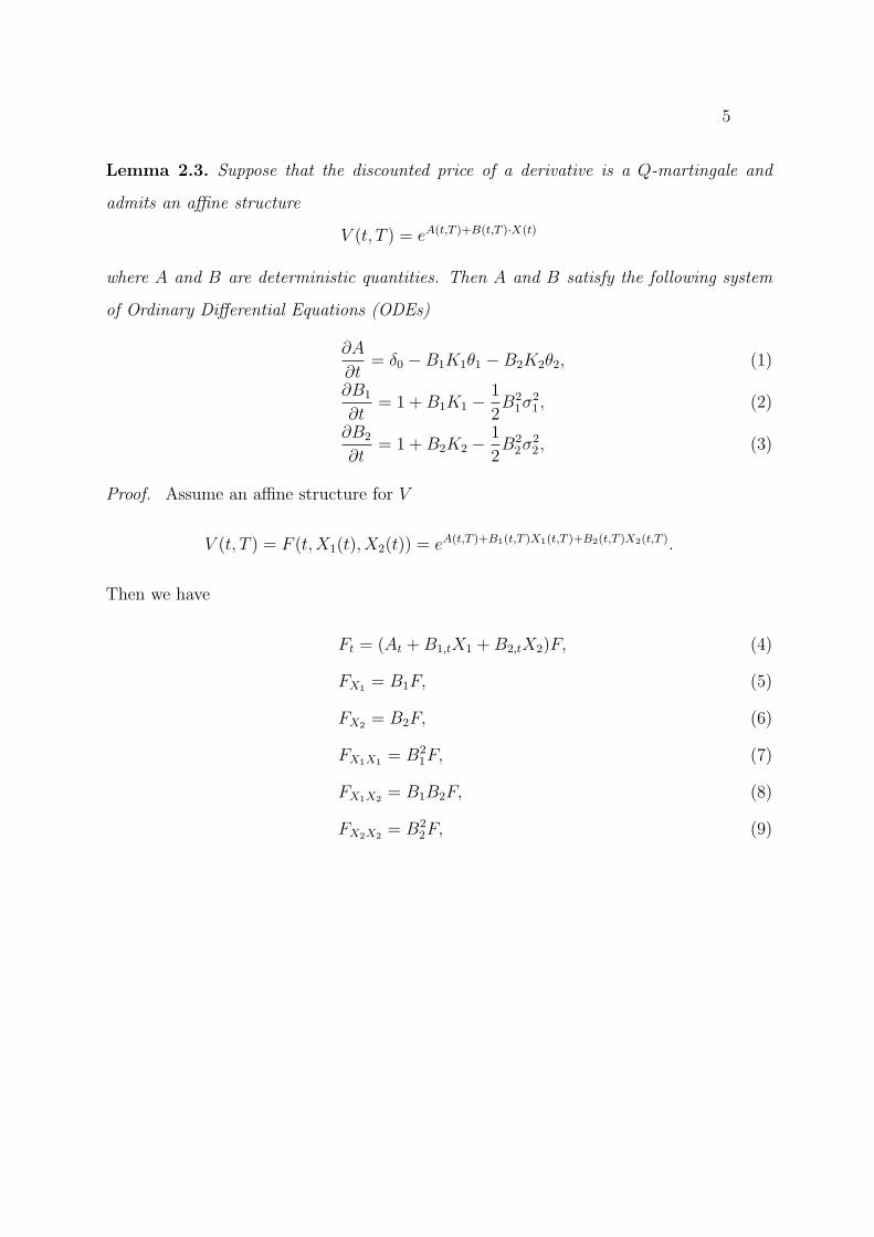
Lemma 2.3. Suppose that the discounted price of a derivative is a Q-martingale and

admits an affine structure

V (t, T ) = eA(t,T )+B(t,T )·X(t)

where A and B are deterministic quantities. Then A and B satisfy the following system

of Ordinary Differential Equations (ODEs)

∂A

∂t= δ0 −B1K1θ1 −B2K2θ2, (1)

∂B1

∂t= 1 +B1K1 −

1

2B2

1σ21, (2)

∂B2

∂t= 1 +B2K2 −

1

2B2

2σ22, (3)

Proof. Assume an affine structure for V

V (t, T ) = F (t,X1(t), X2(t)) = eA(t,T )+B1(t,T )X1(t,T )+B2(t,T )X2(t,T ).

Then we have

Ft = (At +B1,tX1 +B2,tX2)F, (4)

FX1 = B1F, (5)

FX2 = B2F, (6)

FX1X1 = B21F, (7)

FX1X2 = B1B2F, (8)

FX2X2 = B22F, (9)

6

Let D(t) = e−∫ Tt r(s)ds be the discount factor. Then we have

d(DF )

= −rDFdt+DdF

= −rDFdt+D[Ftdt+

FX1dX1 + FX2dX2 +1

2FX1X1dX1dX1 + FX1X2dX1dX2 +

1

2FX2X2dX2dX2]

= D[−rFdt+ Ftdt+ FX1(K1(θ1 −X1)dt+ σ1√X1dW1)+

FX2(K2(θ2 −X2)dt+ σ1√X2dW2) +

1

2FX1X1σ

21X1dt+

1

2FX2X2σ

22X2dt]

= D{[−rF + Ft + FX1K1(θ1 −X1) + FX2K2(θ2 −X2)+

1

2FX1X1σ

21X1 +

1

2FX2X2σ

22X2]dt+ σ1

√X1FX1dW1 + σ2

√X2FX2dW2}

Since DF is a Q-martingale, the drift-term is equal to 0. Thus, we have

−rF + Ft + FX1K1(θ1 −X1) + FX2K2(θ2 −X2) +1

2FX1X1σ

21X1 +

1

2FX2X2σ

22X2 = 0

Therefore,

− (X1 +X2 + δ0) + (At +B1,tX1 +B2,tX2) +B1K1(θ1 −X1) +B2K2(θ2 −X2)

+1

2B2

1σ21X1 +

1

2B2

2σ22X2 = 0

⇒ (−δ0 + At +B1K1θ1 +B2K2θ2)+

(−1 +B1,t −B1K1 +1

2B2

1σ21)X1 + (−1 +B2,t −B2K2 +

1

2B2

2σ22)X2 = 0

Next we obtain the following system

∂A

∂t= δ0 −B1K1θ1 −B2K2θ2, (10)

∂B1

∂t= 1 +B1K1 −

1

2B2

1σ21, (11)

∂B2

∂t= 1 +B2K2 −

1

2B2

2σ22, (12)

7

Theorem 2.4. The price at time t of a zero-coupon bond maturing at time T and with a

unit face value given by

PCIR(t, T ) = eA(t,T )+B(t,T )·X(t)

where

γj =√K2

j + 2σ2j , j = 1, 2

A(t, T ) = −δ0(T − t)−2∑

j=1

Kjθj [2

σ2j

ln(Kj + γj)(e

γj(T−t) − 1)

2γj+

2

Kj − γj(T − t)],

Bj(t, T ) =−2(eγj(T−t) − 1)

(Kj + γj)(eγj(T−t) − 1) + 2γj, j = 1, 2.

Proof. Consider an affine term structure

PCIR(t, T ) = F (t,X1(t), X2(t)) = eA(t,T )+B1(t,T )X1(t,T )+B2(t,T )X2(t,T ).

Then we obtain the following system of ODEs by Lemma 2.3

∂A

∂t= δ0 −B1K1θ1 −B2K2θ2, (13)

∂B1

∂t= 1 +B1K1 −

1

2B2

1σ21, (14)

∂B2

∂t= 1 +B2K2 −

1

2B2

2σ22, (15)

A(T, T ) = B1(T, T ) = B2(T, T ) = 0 (16)

The solution can be derived straightforwardly usng the results discussed in subsection B.2

of the Appendix.

Finally, we calculate the bond moments under the T0-forward measure, which is defined

by

µT0(t, T0, {Ti1 , Ti2 , ..., Tim}) := ET0

[m∏k=1

P (T0, Tik)∣∣∣Ft

].

This is the key to the pricing formula given in next section.

The formula given below can be found in Collin-Dufresne and Goldstein (2002) in [8]

and [12] and we provide a detailed proof of this formula.

8

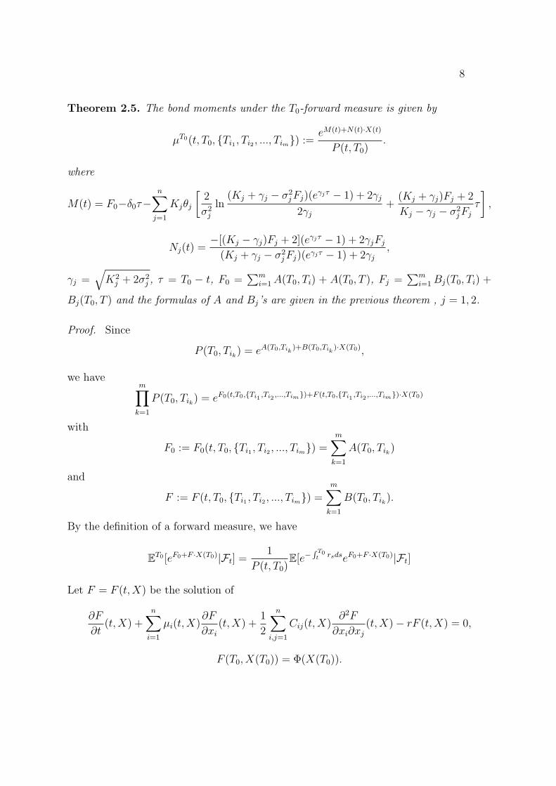
Theorem 2.5. The bond moments under the T0-forward measure is given by

µT0(t, T0, {Ti1 , Ti2 , ..., Tim}) :=eM(t)+N(t)·X(t)

P (t, T0).

where

M(t) = F0−δ0τ−n∑

j=1

Kjθj

[2

σ2j

ln(Kj + γj − σ2

jFj)(eγjτ − 1) + 2γj

2γj+

(Kj + γj)Fj + 2

Kj − γj − σ2jFj

τ

],

Nj(t) =−[(Kj − γj)Fj + 2](eγjτ − 1) + 2γjFj

(Kj + γj − σ2jFj)(eγjτ − 1) + 2γj

,

γj =√K2

j + 2σ2j , τ = T0 − t, F0 =

∑mi=1A(T0, Ti) + A(T0, T ), Fj =

∑mi=1Bj(T0, Ti) +

Bj(T0, T ) and the formulas of A and Bj’s are given in the previous theorem , j = 1, 2.

Proof. Since

P (T0, Tik) = eA(T0,Tik)+B(T0,Tik

)·X(T0),

we havem∏k=1

P (T0, Tik) = eF0(t,T0,{Ti1,Ti2

,...,Tim})+F (t,T0,{Ti1,Ti2

,...,Tim})·X(T0)

with

F0 := F0(t, T0, {Ti1 , Ti2 , ..., Tim}) =m∑k=1

A(T0, Tik)

and

F := F (t, T0, {Ti1 , Ti2 , ..., Tim}) =m∑k=1

B(T0, Tik).

By the definition of a forward measure, we have

ET0 [eF0+F ·X(T0)|Ft] =1

P (t, T0)E[e−

∫ T0t rsdseF0+F ·X(T0)|Ft]

Let F = F (t,X) be the solution of

∂F

∂t(t,X) +

n∑i=1

µi(t,X)∂F

∂xi(t,X) +

1

2

n∑i,j=1

Cij(t,X)∂2F

∂xi∂xj(t,X)− rF (t,X) = 0,

F (T0, X(T0)) = Φ(X(T0)).

9

Assume that F has the form F (t,X) = eM(t)+N(t)·X(t). Then it is easy to show that

M(T0) =m∑i=1

A(T0, Tim), N(T0) =m∑i=1

B(T0, Tim).

Furthermore, the Partial Differential Equation (PDE) above implies that

− (X1 +X2 + δ0) + (Mt +N1,tX1 +N2,tX2) +N1K1(θ1 −X1) +N2K2(θ2 −X2)

+1

2N2

1σ21X1 +

1

2N2

2σ22X2 = 0

⇒ (−δ0 +Mt +N1K1θ1 +N2K2θ2)+

(−1 +N1,t −N1K1 +1

2N2

1σ21)X1 + (−1 +N2,t −N2K2 +

1

2N2

2σ22)X2 = 0

This leads to the following system

∂M

∂t= δ0 −N1K1θ1 −N2K2θ2, (17)

∂N1

∂t= 1 +N1K1 −

1

2N2

1σ21, (18)

∂N2

∂t= 1 +N2K2 −

1

2N2

2σ22, (19)

M(T0) = F0 , N1(T0) = F1 and N2(T0) = F2. (20)

The solution can be derived straightforwardly from the results discussed in subsection B.2

of the Appendix.

2.2 Pricing Swaptions under the CIR2 model

The discussion in this subsection relies heavily on [12]. Consider a swaption with the

expiry T0 and the fixed rate K during a period [T0, TN ]. The price of the underlying swap

is given by

SV (t) =N∑i=0

aiP (t, Ti)

where

a0 = −1 ; ai =P (t, T0)− P (t, TN)∑N

i=1 P (t, TN)(i = 1, ..., N − 1) and aN = 1 +

P (t, T0)− P (t, TN)∑Ni=1 P (t, TN)

.

10

The mth swap moment under the T0-forward measure conditioned on Ft is given by

Mm(t) = ET0

[(N∑i=0

aiP (t, Ti)

)m ∣∣∣Ft

]Note that [

N∑i=0

aiP (t, Ti)

]m=

∑0≤i1,...,im≤N

ai1 ...aim

[m∏k=1

P (T0, Tik)

].

So,

Mm(t) =∑

0≤i1,...,im≤N

ai1 ...aimET0

[m∏k=1


]Remark. Observe that

Mm(t) =∑

0≤k0,...kM≤N,k0+...+kN=m,

ak00 ...akNN ET0

[N∏j=0

P (T0, Tj)kj

∣∣∣Ft

]

By simple combinatorics steps, we obtain

Mm(t) =∑

0≤k0≤...≤kN≤N,k0+...+kN=m,

m!

k0!k1!...kN !ak00 ...a

kNN ET0

[N∏j=0

P (T0, Tj)kj

∣∣∣Ft

]

The algorithm for generating the following collection of sets

{{k0, k1, ..., kN} : 0 ≤ k0, k1, ..., kN ≤ N, k0 + k1 + ...+ kN =M}

is crucial in the implementation of our formulas.

Since the bond moments ET0 [∏m

k=1 P (T0, Tik)|Ft] have closed-form expressions (see

Theorem 2.5), we are able to obtain a closed-form formula for the swaptions. To sum up,

we have the following theorems.

Theorem 2.6. Suppose that the risk-neutral dynamics of the short rates follow the CIR2

model.

r(t) = X1(t) +X2(t) + δ0.


dXi(t) = Ki(θi −Xi(t))dt+ σi√Xi(t)dWi(t) , i = 1, 2.

11

Let cn(t) be the swap cumulants which can be calculated by the swap moments {M1(t), ...,Mn(t)}

and Cn(t) = cn(t)P (t, T0)n for n ≥ 1. Let q0 = 1, q1 = q2 = 0 and

qn =

[n3]∑

m=1

∑k1,...km≥3,

k1+...+km=n,

Ck1 ...Ckm

m!k1!...km!√C2

n , n ≥ 3.

The risk-neutral price of the T0 × (TN − T0)-receiver swaption SOV (t;T0, Tn) is given by

SOV (t;T0, Tn) = C1N

(C1√C2

)+√C2ϕ

(C1√C2

)[1 +

∞∑k=3

(−1)kqkHk−1

(C1√C2

)].

2.3 Numerical results

In this subsection, we provide numerical results for the method of pricing swaptions

discussed in the last subsection. That is, we consider the following parameters in the

CIR2 model:

Parameters V alues

S0 1

δ0 0.02

κ1 0.2

κ2 0.2

θ1 0.03

θ2 0.01

σ1 0.04

σ2 0.02

X1(0) 0.04

X2(0) 0.02

We consider N = 5, 00, 000 scenarios and 12 time steps per year for a Monte-Carlo

simulation of the call option prices. We approximate the price of the call option using

only first N terms in the Gram-Charlier expansions and denote them by GC(N). The

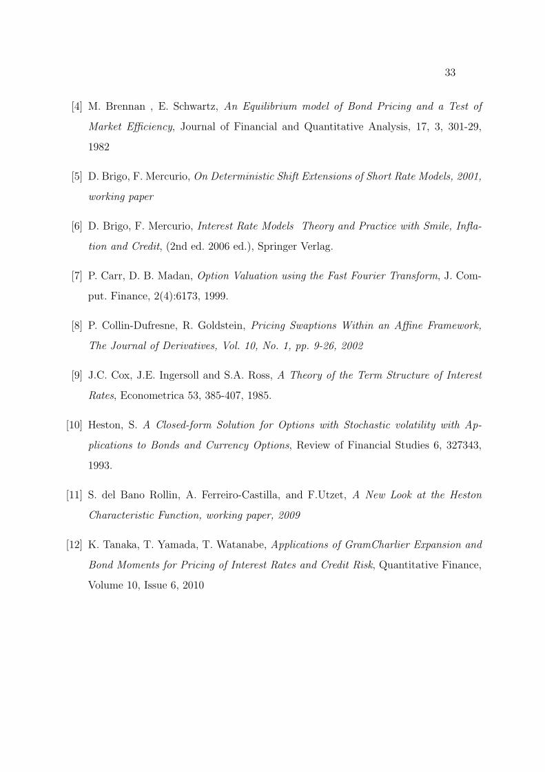
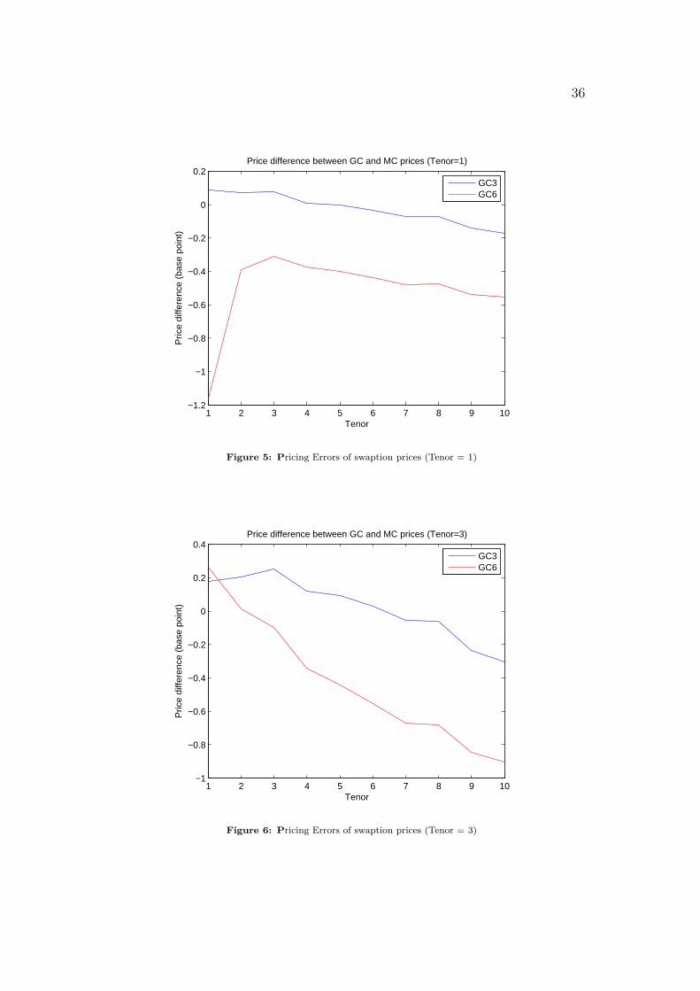
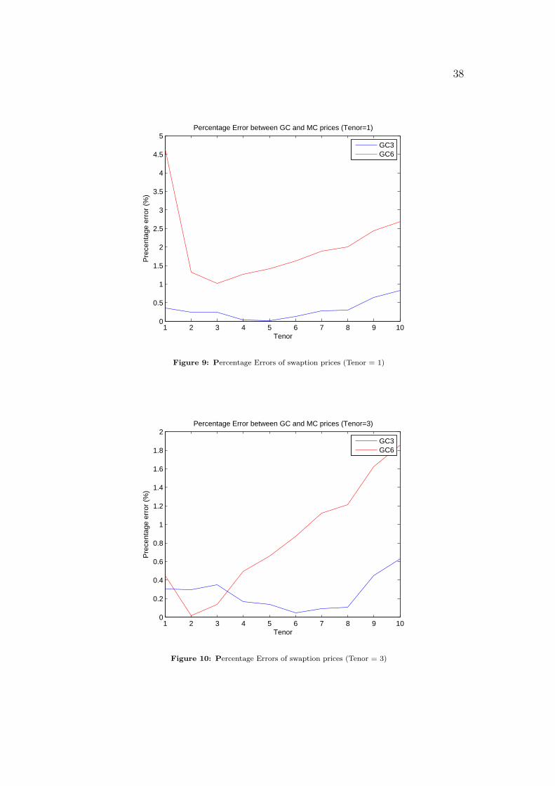
numerical results are summarized in Figures 1 - 12. From these figures, we see that the

12

GC3 , which is the Gram-Charlier expansions up to the third cumulants, is generally more

accurate than GC6, which is the Gram-Charlier expansions up to the sixth cumulants.

GC6 is slightly more accurate in the short tenor swaptions, but substantially less accurate

for long tenor swaptions.

In order to confirm that the result given above is not merely an artifact of the selected

configuration of parameter values, we repeat the testing procedure by using another set

of parameter values:

Parameters V alues

S0 1

δ0 −0.02

κ1 0.05

κ2 0.5

θ1 0.085

θ2 0.01

σ1 0.08

σ2 0.05

X1(0) 0.01

X2(0) 0.01

The numerical results are summarized in Figures 13 - 24. From these figures, we again

find that the GC3 is generally more accurate than GC6. Increasing the terms in the

Gram-Charlier expansion does not appear to increase the accuracy of the approximation.

This is due to the fact that the Gram-Charlier expansions is an orthogonal series. Also

we note that it is difficult to obtain a precise estimate of the error under this approach.

13

2.4 Pricing Swaptions under the CIR2++ model

In this subsection, we discuss how the Gram-Charlier expansions can be used to calculate

swaption prices under an extended version of the two-factor CIR (CIR2) model, known

as the CIR2++ model. Recall that the CIR2 model is specified as

dX1(t) = K1(θ1 −X1(t))dt+ σ1√X1(t)dW1(t);

dX2(t) = K2(θ1 −X2(t))dt+ σ2√X2(t)dW2(t)

with the initial conditions given by

X(0) = (X1(0), X2(0)) are given,

where W1, W2 are independent Q-Brownian motions.

In the CIR2++ model (See Brigo and Mercurio (2001) in [5]), the short rate, instead,

is given by

r(t) = X1(t) +X2(t) + ψ(t).

where ψ(t) is chosen, so as to fit the initial zero-coupon curve.

Let fj be the the instantaneous forward rate given by the jth SDE, j = 1, 2.

Let fM be the market instantaneous forward rate. Then

ψ(t) = fM(0, t)− f1(0, t)− f2(0, t).

Next we define the following

Φ(u, v) =PM(0, v)

PM(0, u)

PCIR(0, u)

PCIR(0, v)

where PM is the market discount factor.

The price at time t of a zero-coupon bond maturing at time T and with a unit face

value is given by

P (t, T ) = Φ(t, T )PCIR(t, T )

14

where

PCIR(t, T ) = eA(t,T )+B(t,T )·X(t)

γj =√K2

j + 2σ2j , j = 1, 2

A(t, T ) = −2∑

j=1

Kjθj [2

σ2j

ln(Kj + γj)(e

γj(T−t) − 1)

2γj+

2

Kj − γj(T − t)];

Bj(t, T ) =−2(eγj(T−t) − 1)

(Kj + γj)(eγj(T−t) − 1) + 2γj, j = 1, 2

So, we can write

P (t, T ) =PM(0, T )

PM(0, t)

[PCIR(0, t)

PCIR(0, T )PCIR(t, T )

].

It is clear that

P (0, T ) =PM(0, T )

PM(0, t)

[PCIR(0, t)

PCIR(0, T )PCIR(t, T )

]= PM(0, T ).

Therefore, the discount factors derived from the model should match the initial term

structure.

Consider a swaption with the expiry T0 and the fixed rate K during a period [T0, TN ].

The price of the underlying swap is given by

SV (t) =N∑i=0

aiP (t, Ti)

where

a0 = −1 ; ai =P (t, T0)− P (t, TN)∑N

i=1 P (t, TN)(i = 1, ..., N − 1) and aN = 1 +

P (t, T0)− P (t, TN)∑Ni=1 P (t, TN)

.

In particular, at time t = 0, the swap price is given by

SV (0) =N∑i=0

aiP (0, Ti) =N∑i=0

aiPM(0, Ti)

where

a0 = −1 ;

15

ai =PM(0, T0)− PM(0, TN)∑N

i=1 PM(0, TN)

(i = 1, ..., N − 1) and aN = 1 +PM(0, T0)− PM(0, TN)∑N

i=1 PM(0, TN)

.

The mth swap moment under the T0-forward measure conditioned on Ft is given by

M∗m(t) = ET0 [{

N∑i=0

aiP (t, Ti)}m|Ft]

Note that [N∑i=0

aiP (t, Ti)

]m=

∑0≤i1,...,im≤N

ai1 ...aim

[m∏k=1

P (T0, Tik)

].

So,

M∗m(t) =

∑0≤i1,...,im≤N

ai1 ...aimET0

[m∏k=1


]We have to calculate the bond moment under the T0-forward measure, which is defined

as

µT0(t, T0, {Ti1 , Ti2 , ..., Tim}) := ET0

[m∏k=1


].

Observe that

P (T0, Tik) =PM(0, Tik)

PM(0, T0)

[PCIR(0, T0)

PCIR(0, Tik)PCIR(T0, Tik)

].

We have

M∗m(t) =

∑0≤i1,...,im≤N

ai1 ...aimET0

[m∏k=1

PM(0, Tik)

PM(0, T0)

[PCIR(0, T0)

PCIR(0, Tik)PCIR(T0, Tik)

] ∣∣∣∣∣Ft

]

=

(PCIR(0, T0)

PM(0, T0)

)m ∑0≤i1,...,im≤N

ai1 ...aim

m∏k=1

PM(0, Tik)

PCIR(0, Tik)ET0

[m∏k=1

PCIR(T0, Tik)∣∣∣Ft

]

=

(PCIR(0, T0)

PM(0, T0)

)m ∑0≤i1,...,im≤N

a∗i1 ...a∗imE

T0

[m∏k=1

PCIR(T0, Tik)∣∣∣Ft

],

where a∗ik = aikPM (0,Tik

)

PCIR(0,Tik)

Therefore, we have a closed-form formula for the swaption prices under the CIR2++

model.

16

Theorem 2.7. Suppose that the risk-neutral dynamics of the short rates follow the CIR2++

model.

r(t) = X1(t) +X2(t) + ψ(t).


dXi(t) = Ki(θi −Xi(t))dt+ σi√Xi(t)dWi(t) , i = 1, 2

and ψ(t) is chosen, so as to fit the initial zero-coupon curve.

Let c∗n(t) be the swap cumulants which can be calculated by the swap moments {M∗1 (t),

...,M∗n(t)} and C∗

n(t) = c∗n(t)P (t, T0)n for n ≥ 1. Put q0 = 1, q1 = q2 = 0 and

qn =

[n3]∑

m=1

∑k1,...km≥3,

k1+...+km=n,

C∗k1...C∗

km

m!k1!...km!√C∗

2

n , n ≥ 3.

The risk neutral price of the T0 × (TN − T0)-receiver swaption SOV (t;T0, Tn) is given by

SOV (t;T0, Tn) = C∗1N

(C∗

1√C∗

2

)+√C∗

2ϕ

(C∗

1√C∗

2

)[1 +

∞∑k=3

(−1)kqkHk−1

(C∗

1√C∗

2

)].

3 Applications of Gram-Charlier expansions to Gen-

eral Models

In Theorem A.2, we provide a procedure to calculate the survival function (hence, the

cumulative distribution function) and the truncated first moment of a random variable

when its cumulants (or moments) are known. Theoretically speaking, we are able to

calculate the prices of the European-type derivatives of any diffusion process if we are

able to calculate its moments. In this section, we discuss a general procedure with worked

examples in details.

3.1 A Toy Example: Black-Scholes Model

In this subsection, we show how to use Gram-Charlier expansions to calculate the price

of a European call option under the standard Black-Scholes (1973) model in [3]. The

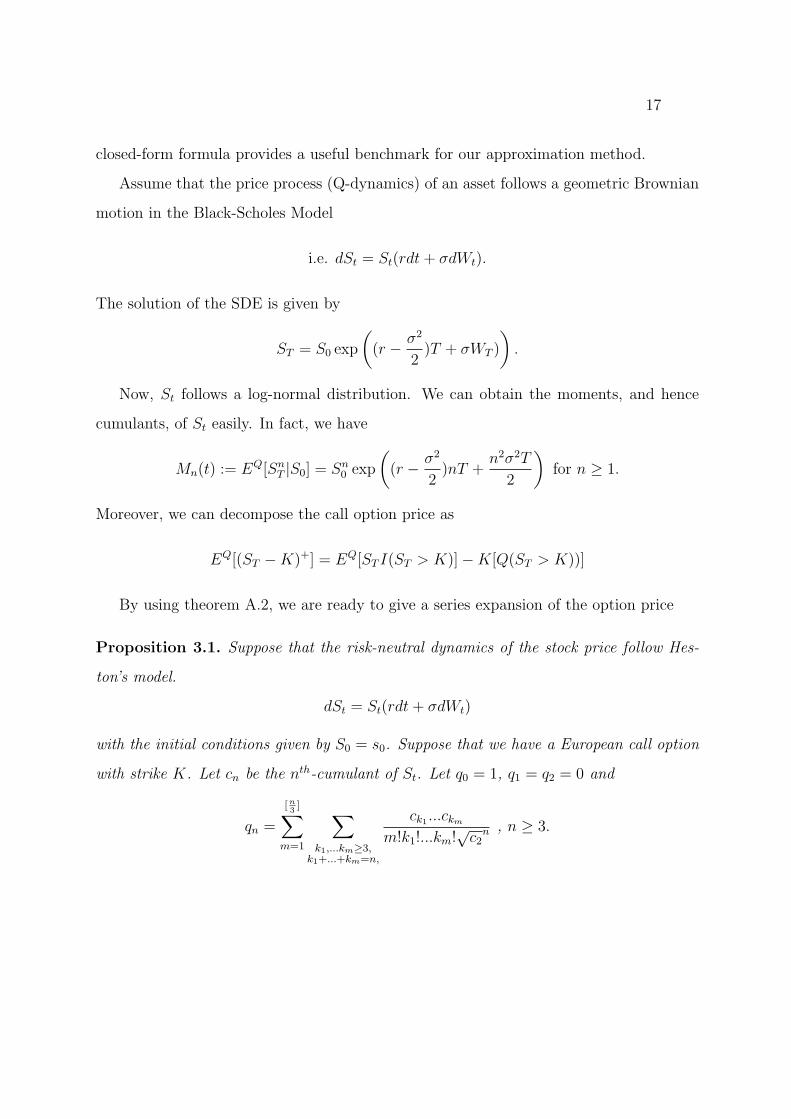
17

closed-form formula provides a useful benchmark for our approximation method.

Assume that the price process (Q-dynamics) of an asset follows a geometric Brownian

motion in the Black-Scholes Model

i.e. dSt = St(rdt+ σdWt).

The solution of the SDE is given by

ST = S0 exp

((r − σ2

2)T + σWT )

).

Now, St follows a log-normal distribution. We can obtain the moments, and hence

cumulants, of St easily. In fact, we have

Mn(t) := EQ[SnT |S0] = Sn

0 exp

((r − σ2

2)nT +

n2σ2T

2

)for n ≥ 1.

Moreover, we can decompose the call option price as

EQ[(ST −K)+] = EQ[ST I(ST > K)]−K[Q(ST > K))]

By using theorem A.2, we are ready to give a series expansion of the option price

Proposition 3.1. Suppose that the risk-neutral dynamics of the stock price follow Hes-

ton’s model.

dSt = St(rdt+ σdWt)

with the initial conditions given by S0 = s0. Suppose that we have a European call option

with strike K. Let cn be the nth-cumulant of St. Let q0 = 1, q1 = q2 = 0 and

qn =

[n3]∑

m=1

∑k1,...km≥3,

k1+...+km=n,

ck1 ...ckmm!k1!...km!

√c2

n , n ≥ 3.

18

Then the price of the call option price is equal to the following infinite sum

√c2ϕ

(c1 −K√

c2

)+ c1N

(c1 −K√

c2

)+

∞∑n=3

(−1)n−1qnϕ

(c1 −K√

c2

) [KHn−1

(c1 −K√

c2

)−√C2Hn−2

(c1 −K√

c2

)]

−K

[N

(c1 − a√

c2

)+

∞∑k=3

(−1)k−1qkHk−1

(c1 − a√

c2

)ϕ

(c1 − a√

c2

)].

In the rest of this subsection, we present the result of a test on our Gram-Charlier

approach. Here is a list of parameters used for the model:

Parameters V alues

S0 100

K {80, 80.1, ..., 119.9, 120.0}

σ 0.03

T 1 or 2

r 0.05

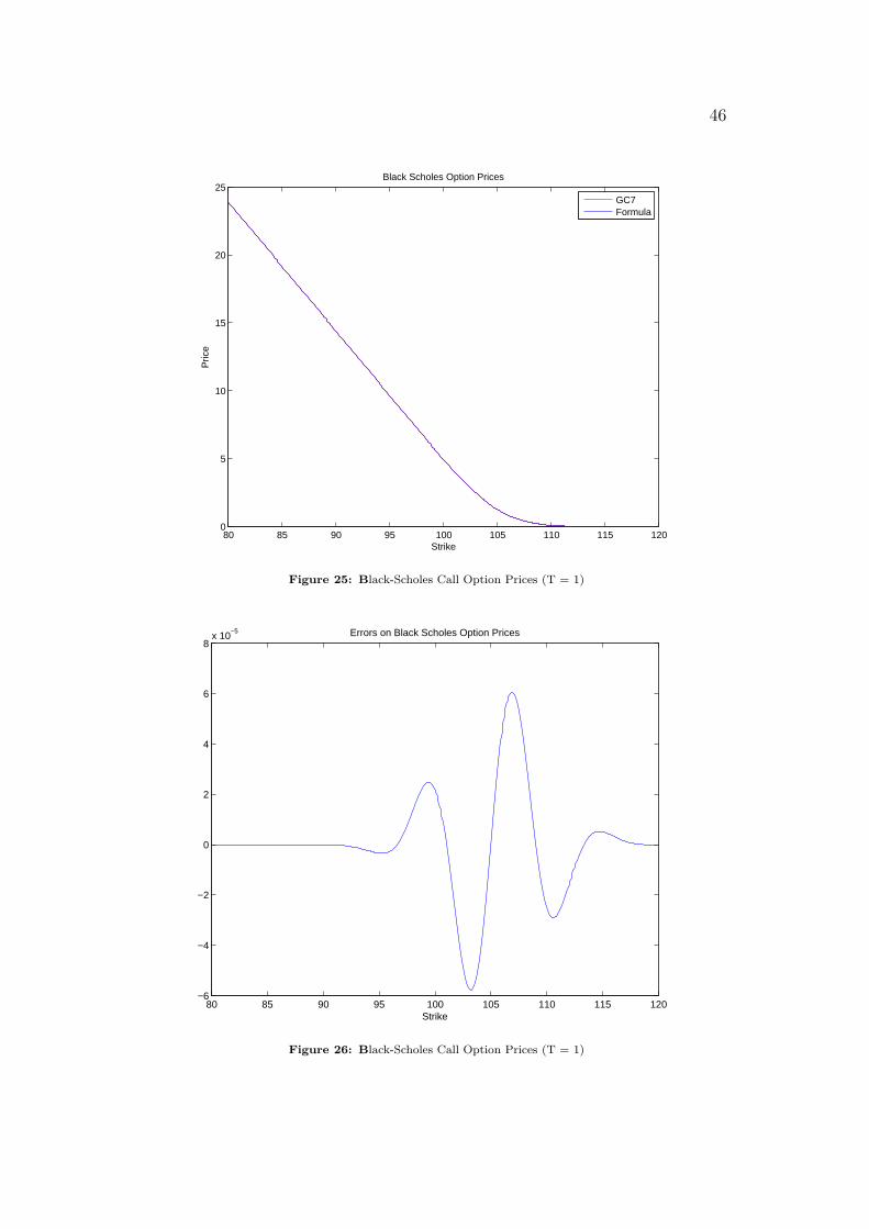
We use 7 terms in the Gram-Charlier expansion. The results are given in Figures 25

- 30. From these figures, we see that that the (relative) errors are generally very small.

Specifically the errors are smaller for the out-of-money options. Also, it is more accurate

if the time-to-expiry is longer.

3.2 Application to a Simplified Version of the Brennan and

Schwarz Model

The Brennan and Schwarz (1982) model in (See [4]) is a two-factor model of interest rates.

It is specified as drt = (a1 + b1(lt − rt))dt+ σ1rtdW1t

dlt = lt(a2 − b2rt + c2lt)dt+ σ2ltdW2t

(21)

19

where ai’s and bi’s are constants.

To make the discussion more concrete, we assume that lt is a constant process and

rewrite the process of rt as

drt = κ(θ − rt)dt+ σrtdWt (22)

The first step of our approximation process is to calculate the moments of rt. We first

apply the Ito’s lemma to the process (rnt ):

drnt = nrn−1t drt +

n(n− 1)

2rn−2t (drt)

2

= nrn−1t [κ(θ − rt)dt+ σrtdWt] +

n(n− 1)

2rn−2t σ2r2t dt

= [nκθrn−1t − nκrnt ]dt+

n(n− 1)

2rnt σ

2dt+ σrtdWt.

In the integral from, we have

rnt − rn0 = nκθ

∫ t

0

rn−1s ds+ [

(n− 1)σ2

2− κ]

∫ t

0

nrns ds+ σ

∫ t

0

rsdWs.

Assume that the parameters in 22 behave well enough, so that rt is square-integrable.

The last term becomes a martingale. Let Fn(t) = E[rnt ]. By Fubini’s theorem, we have

Fn(t) = rn0 + nκθ

∫ t

0

Fn−1(s)ds+ [(n− 1)σ2

2− κ]

∫ t

0

nFn(s)ds.

In other words, Fn(t) can be solved recursively in the following system of ODEs:

F ′n(t) = nκθFn−1(t) + [

(n− 1)σ2

2− κ]Fn(t) ; Fn(0) = rn0 for n ≥ 1.

In the rest of this subsection, we present the result of a test on our Gram-Charlier

approach. Here is a list of parameters we use for the model:

20

Parameters V alues

r0 0.06

r {0.001, 0.002, ...0.1}

T 5

κ 0.2

θ 0.05

σ 0.115

We approximate the distribution of rt by using Theorem A.2. The moments of rt are

calculated by solving the system of ODEs discussed above with Mathematica. We use 7

terms in the Gram-Charlier expansion. The results are given in Figures 31 and 32. From

these figures, we see that the approximation provides a fairly good fit to the model. The

error in the middle region is relatively higher, and up to 0.02. This error is likely to be

acceptable from the perspective of risk management.

4 Pricing Call Options under Heston’s Model using

Gram-Charlier expansions

4.1 Introduction to Heston’s Model of Stochastic Volatility

We assume that the risk-neutral dynamics of the stock price follows Heston’s (1993)

stochastic volatility model in [10]. It is given by the following system of SDEsdSt = St(rdt+√VtdW

1t )

dVt = κ(θ − Vt)dt+ σ√VtdW

2t

(23)

with the initial conditions given by S0 = s0 and V0 = v0 ≥ 0, where κ, θ, σ > 0 and

dW 1t dW

2t = ρdt, ρ ∈ [−1, 1].

Let Xt = lnSt − rt be the logarithm of the discounted stock price. By Ito’s lemma,

we have

dXt = −rdt+dSt

St

− 1

2S2t

(dSt · dSt) = −1

2Vtdt+

√VtdW

1t ,

21

with the initial condition given by Xo = xo = lnS0.

Thus, we can transform the system (28) into the following systemdXt = −12Vtdt+

√VtdW

1t


2t

(24)

with the initial conditions given by X0 = x0 and V0 = v0 ≥ 0.

We can show that the moment generating function of Xt (See [11]) is given by

Mt(u) = E[euXt ] = ex0u

(e(κ−σρt)/2

cosh(P (u)t/2) + (κ− σρu) sinh(P (u)t/2)/P (u)

)2κθ/σ2

· exp(−v0

(u− u2) sinh(P (u)t/2)/P (u)cosh(P (u)t/2) + (κ− σρu) sinh(P (u)t/2)/P (u)

)(25)

where

P (u) =√(κ− ρcu)2 + c2(u− u2).

Hence, the cumulants of Xt can be calculated by

cn =dn

dun[lnMt(u)]

∣∣∣∣u=0

for n = 1, 2, ...

In practice, the higher derivatives in the expression can be calculated reasonably fast

by using any available symbolic calculation software.

4.2 Calculating Truncated Moment Generating Function using

Gram-Charlier Expansions

Proposition 4.1. Let Y be a random variable, such that it has a continuous density

function f(x) and finite cumulants (ck)k∈N. Let q0 = 1, q1 = q2 = 0 and

qn =

[n3]∑

m=1

∑k1,...km≥3,

k1+...+km=n,


√c2

n , n ≥ 3.

Suppose that eaY is integrable where a ∈ R. Then the following results are obtained

22

(a) The truncated below moment generating function of Y is given by

E[eaxI(Y ≤ K)] = eaC1

∞∑n=0

qnIn

(K − C1√

C2

, a√C2

)(26)

where In = In(x, a) satisfies the following recurrence

I0(x, a) = eb2

2 N(x− a) ; In(x, b) = aIn−1(x, a)−Hn−1(x)ϕ(x)eax.

(b) The truncated above moment generating function of Y is given by

E[eaxI(Y ≥ K)] = eaC1

∞∑n=0

qnJn

(K − C1√

C2

, a√C2

)(27)

where Jn = Jn(x, a) satisfies the following recurrence

J0(x, a) = eb2

2 N(a− x) ; Jn(x, a) = aJn−1(x, a) +Hn−1(x)ϕ(x)eax.

Proof. We first prove part (a). Recall that

f(x) =∞∑n=0

qn√c2Hn

(x− c1√

c2

)ϕ

(x− c1√

c2

).

We have

E[eaxI(Y ≤ K)] =

∫ K

−∞eax

∞∑n=0

qn√c2Hn

(x− c1√

c2

)ϕ

(x− c1√

c2

)dx

=∞∑n=0

qn√c2

∫ K

−∞eaxHn

(x− c1√

c2

)ϕ

(x− c1√

c2

)dx

=∞∑n=0

qn√c2

∫ K−C1√C2

−∞Hn(y)ϕ(y)e

a√C2y+aC1

√C2dy

=∞∑n=0

qneaC1

∫ K−C1√C2

−∞Hn(y)ϕ(y)e

a√C2ydy

Let In(x, a) =∫ x

∞Hn(y)ϕ(y)eaydy. Write In := In(x, a) for convenience. When n = 0,

23

we have

I0 =

∫ x

−∞H0(y)ϕ(y)e

aydy

=

∫ x

−∞ϕ(y)eaydy

=1√2π

∫ x

−∞e−

y2

2 eaydy

=e

a2

2

√2π

∫ x

−∞e−

(y−a)2

2 dy

= ea2

2 N(x− a).

Note that

D[(Dn−1ϕ(x))eax] = [Dnϕ(x)]eax + aeax[Dn−1ϕ(x)].

We have

D[(−1)n−1Hn−1(x)ϕ(x)eax] = (−1)nHn(x)ϕ(x)e

ax + (−1)n−1aHn−1(x)ϕ(x)eax.

It follows that

Hn−1(x)ϕ(x)eax = −

∫ x

−∞Hn(y)ϕ(y)e

aydy + a

∫ x

−∞Hn−1(y)ϕ(y)e

aydy.

Hence,

In = aIn−1 −Hn−1(x)ϕ(x)eax.

Therefore, the proof of (a) is completed.

24

For the proof of part (b), we have

E[eaxI(Y ≥ K)] =

∫ ∞

K

eax∞∑n=0

qn√c2Hn

(x− c1√

c2

)ϕ

(x− c1√

c2

)dx

=∞∑n=0

qn√c2

∫ ∞

K

eaxHn

(x− c1√

c2

)ϕ

(x− c1√

c2

)dx

=∞∑n=0

qn√c2

∫ ∞

K−C1√C2

Hn(y)ϕ(y)ea√C2y+aC1

√C2dy

=∞∑n=0

qneaC1

∫ ∞

K−C1√C2

Hn(y)ϕ(y)ea√C2ydy

Let Jn(x, a) =∫∞xHn(y)ϕ(y)e

aydy. Write Jn := Jn(x, a) for convenience. When n = 0,

we have

J0 =

∫ ∞

x

H0(y)ϕ(y)eaydy

=

∫ ∞

x

ϕ(y)eaydy

=1√2π

∫ ∞

x

e−y2

2 eaydy

=e

a2

2

√2π

∫ ∞

x

e−(y−a)2

2 dy

= ea2

2 N(a− x).

Note that

D[(Dn−1ϕ(x))eax] = [Dnϕ(x)]eax + aeax[Dn−1ϕ(x)].

We have

D[(−1)n−1Hn−1(x)ϕ(x)eax] = (−1)nHn(x)ϕ(x)e

ax + (−1)n−1aHn−1(x)ϕ(x)eax.

It follows that

−Hn−1(x)ϕ(x)eax = −

∫ ∞

x

Hn(y)ϕ(y)eaydy + a

∫ ∞

x

Hn−1(y)ϕ(y)eaydy.

25

Hence,

Jn = aJn−1 +Hn−1(x)ϕ(x)eax.

Therefore, the proof of (b) is completed.

4.3 Pricing Call Options under the Heston model

Let Xt = lnSt− rt be the logarithm of the discounted stock price. We have eXt = e−rtSt.

The price of the European call option with strike K is given by

C = E[e−rt(St −K)+] = E[(eXt − e−rtK)+].

Put k = lnK − rt. We may rewrite the price as

C = E[(eXt − ek)+].

Hence, the price of the call option can be calculated by the following formula

C = E[eXtI(Xt > k)]− ekE[I(Xt > k)].

The first term on the right-hand side of the above expression is just a truncated

Moment Generating Function (MGF) which can be calculated via equation (27) and the

second term can be calculated by the formula given in Theorem A.2. Therefore, we are

able to calculate the price of any European call option whenever the moments (or the

cumulants) of the log-prices possess analytical formulas.

To sum up, we have the following formula:

Theorem 4.2. Suppose that the risk-neutral dynamics of the stock price follow Heston’s

(1993) stochastic volatility model.dSt = St(rdt+√VtdW

1t )


2t

(28)

with the initial conditions given by S0 = s0 and V0 = v0 ≥ 0, where κ, θ, σ > 0 and

dW 1t dW

2t = ρdt, ρ ∈ [−1, 1]. Suppose that we have a European call option with strike K.

26

Let Xt = lnSt − rt, k = lnK − rt and cn be the nth-cumulant of Xt.

Let q0 = 1, q1 = q2 = 0 and

qn =

[n3]∑

m=1

∑k1,...km≥3,

k1+...+km=n,


√c2

n , n ≥ 3.

The price of the call option price is equal to the following infinite sum

ec1∞∑n=0

qnJn

(k − c1√

c2,√c2

)−ek

[N

(c1 − k√

c2

)+

∞∑n=3

(−1)n−1qnHn−1

(c1 − k√

c2

)ϕ

(c1 − k√

c2

)]

where Jn = Jn(x, a) satisfies the following recurrence:

J0(x, a) = eb2

2 N(a− x) ; Jn(x, a) = aJn−1(x, a) +Hn−1(x)ϕ(x)eax.

4.4 A Monte-Carlo Simulation Method for the Heston Model

In order to investigate the accuracy of our result, we calculate the options prices based on

a Monte-Carlo method. Note that the second equation of the Heston system is a CIR-type

mean-reverting process. Thus it is tempting to use an exact simulation method since the

distribution of Vt is known as a non-central chi-square distribution. However, it turns out

to be very cumbersome to include the correlation of the Brownian motions because the

Cholesky decomposition is not applicable in this case.

Inspired by the result reported in Alfonsi (2005) in [1], we use the implicit scheme for

(√Vt) and an exact simulation for (St). To make it clear, we first obtain the SDE for

(√Vt) by Ito’s lemma

d√Vt =

κθ − σ2/4

2√Vt

dt− κ

2

√Vtdt+

σ

2dW 2

t .

Let the time grid be {t0, ..., tn} where t0 = 0, tn = T and ti =iTnfor i = 1, ..n. We obtain

the following equation by impliciting the drift term:

√Vti+1

−√Vti =

(κθ − σ2/4

2√Vti+1

− κ

2

√Vti+1

)T

n+σ

2(Wti+1

−Wti).

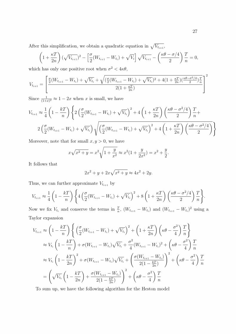
27

After this simplification, we obtain a quadratic equation in√Vti+1

,(1 +

κT

2n

)(√Vti+1

)2 −[σ2(Wti+1

−Wti) +√Vi

]√Vti+1

−(κθ − σ/4

2

)T

n= 0,

which has only one positive root when σ2 < 4κθ,

Vti+1=

σ2(Wti+1

−Wti) +√Vti +

√(σ2(Wti+1

−Wti) +√Vti)

2 + 4(1 + κT2n)(κθ−σ2/4

2)Tn

2(1 + κT2n)

2

Since 1(1+x)2

≈ 1− 2x when x is small, we have

Vti+1≈ 1

4

(1− kT

n

){2(σ2(Wti+1

−Wti) +√Vti

)2+ 4

(1 +

κT

2n

)(κθ − σ2/4

2

)T

n+

2(σ2(Wti+1

−Wti) +√Vti

)√(σ2(Wti+1

−Wti) +√Vti

)2+ 4

(1 +

κT

2n

)(κθ − σ2/4

2

)}Moreover, note that for small x, y > 0, we have

x√x2 + y = x2

√1 +

y

x2≈ x2(1 +

y

2x2) = x2 +

y

2.

It follows that

2x2 + y + 2x√x2 + y ≈ 4x2 + 2y.

Thus, we can further approximate Vti+1by

Vti+1≈ 1

4

(1− kT

n

){4(σ2(Wti+1

−Wti) +√Vti

)2+ 8

(1 +

κT

2n

)(κθ − σ2/4

2

)T

n

}.

Now we fix Vti and conserve the terms in Tn, (Wti+1

−Wti) and (Wti+1−Wti)

2 using a

Taylor expansion

Vti+1≈(1− kT

n

){(σ2(Wti+1

−Wti) +√Vti

)2+

(1 +

κT

2n

)(κθ − σ2

4

)T

n

}

≈ Vti

(1− kT

n

)+ σ(Wti+1

−Wti)√Vti +

σ2

4(Wti+1

−Wti)2 +

(κθ − σ2

4

)T

n

≈ Vti

(1− kT

2n

)2

+ σ(Wti+1−Wti)

√Vti +

(σ(Wti+1

−Wti)

2(1− kT2n)

)2

+

(κθ − σ2

4

)T

n

=

(√Vti

(1− kT

2n

)+σ(Wti+1

−Wti)

2(1− kT2n)

)2

+

(κθ − σ2

4

)T

n

To sum up, we have the following algorithm for the Heston model

28

1. Set S ← s0, V ← v0.

2. Generate a pair of independent Z1, Z2 ∼ N(0, 1).

3. Let U1 =√

1− ρ2Z1 + ρZ2 and U2 = Z2.

4. Generate

V ←

√V (1− kT

2n

)+σ(√

TnU2)

2(1− kT2n)

2

+

(κθ − σ2

4

)T

n.

5. Generate

S ← exp

((r − σ2

2

)T

n+√V

√T

nU1

).

We assume the following parameters in the Heston model to demonstrate the mean

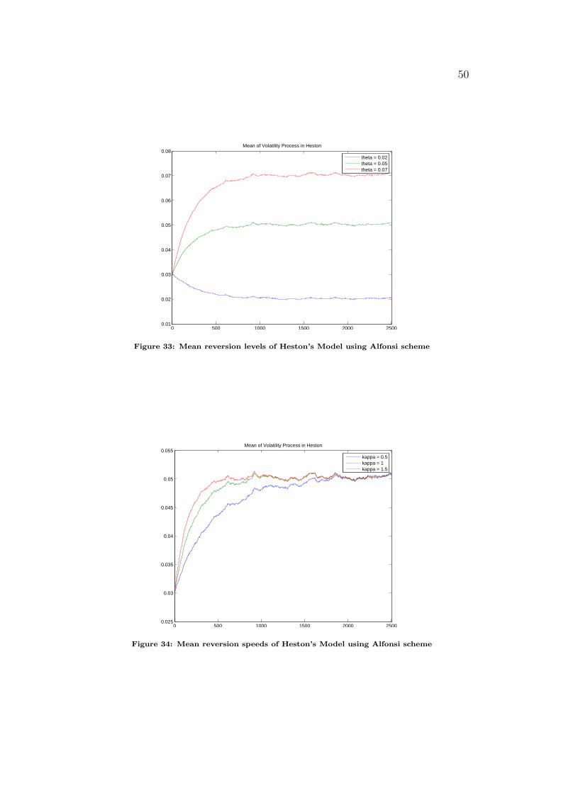
behavior of the scenarios generated by the Alfonsi’s scheme:

Parameters V alues

S0 100

V0 0.03

κ 0.5, 1, 1.5

θ 0.05

σ 0.30

ρ −0.45

T 10

r 0.04

We use 250 time steps per year and generate 10,000 scenarios.The results are given in

Figures 33 and 34.

5 Numerical results

Next we consider the following parameters in the Heston model:

29

Parameters V alues

S0 100

V0 0.03

K {50, 51, ..., 149, 150}

κ 0.15

θ 0.05

σ 0.05

ρ −0.55

T 1

r 0.04

We take N = 1, 000, 000 Scenarios and 250 time steps per year for the Monte-Carlo

simulation of the call option prices. We approximate the price of the call option using

only first N terms in the Gram-Charlier expansions and denote them by GC(N). We also

study GC(ND) where N = 3, 4, 5. They are just GC7’s with CN+1 = ... = C7 = 0 where

N = 3, 4, 5.

Since the Fourier Transform (FT) approach is widely used in calculating the option

price under the Heston model, we also incorporate the FT results in our graph for com-

parison purpose.

Selected Numerical results:

Value/ Strike 50 80 90 100 110 120 150

MC 51.9653 23.7206 15.5576 9.0765 4.6458 2.0766 0.0872

FT 51.9612 23.7138 15.5526 9.0761 4.6510 2.0835 0.0880

GC3 51.9603 23.7141 15.5635 9.0932 4.6667 2.0889 0.0694

GC4 51.9608 23.7216 15.5510 9.0620 4.6424 2.0883 0.0893

GC5 51.9608 23.7199 15.5469 9.0612 4.6469 2.0939 0.0871

GC3D 51.9604 23.7076 15.5648 9.1068 4.6755 2.0834 0.0674

GC4D 51.9609 23.7154 15.5523 9.0750 4.6508 2.0831 0.0874

GC5D 51.9609 23.7136 15.5482 9.0742 4.6553 2.0887 0.0852

30

We see from Figures 35 - 38 that the (relative) errors are generally very small for the

out-of-money options. The GC4D and GC5D approach are generally better than other

approximations. They occasionally outperform the FT approach.

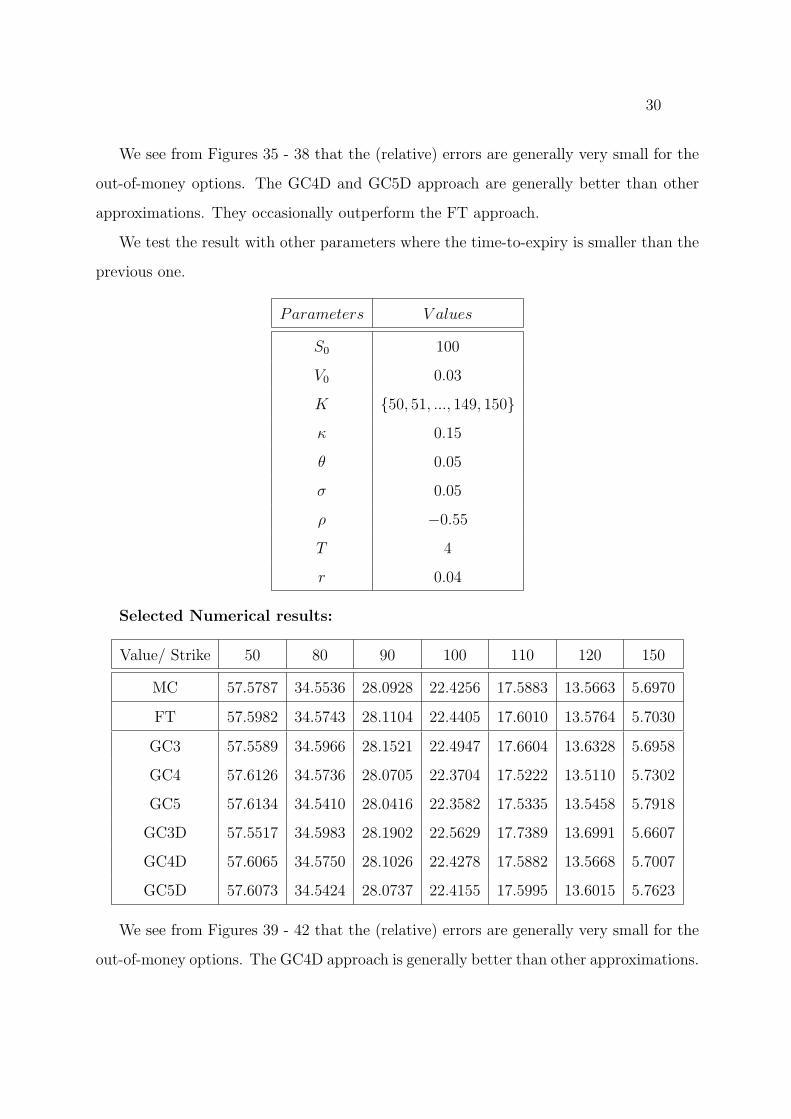
We test the result with other parameters where the time-to-expiry is smaller than the

previous one.

Parameters V alues

S0 100

V0 0.03

K {50, 51, ..., 149, 150}

κ 0.15

θ 0.05

σ 0.05

ρ −0.55

T 4

r 0.04

Selected Numerical results:

Value/ Strike 50 80 90 100 110 120 150

MC 57.5787 34.5536 28.0928 22.4256 17.5883 13.5663 5.6970

FT 57.5982 34.5743 28.1104 22.4405 17.6010 13.5764 5.7030

GC3 57.5589 34.5966 28.1521 22.4947 17.6604 13.6328 5.6958

GC4 57.6126 34.5736 28.0705 22.3704 17.5222 13.5110 5.7302

GC5 57.6134 34.5410 28.0416 22.3582 17.5335 13.5458 5.7918

GC3D 57.5517 34.5983 28.1902 22.5629 17.7389 13.6991 5.6607

GC4D 57.6065 34.5750 28.1026 22.4278 17.5882 13.5668 5.7007

GC5D 57.6073 34.5424 28.0737 22.4155 17.5995 13.6015 5.7623

We see from Figures 39 - 42 that the (relative) errors are generally very small for the

out-of-money options. The GC4D approach is generally better than other approximations.

31

It outperforms the FT approach when the option is in the at-time money region. Increas-

ing the number of terms in the approximation formula does not appear to increase the

accuracy systematically since the Gram-Charlier expansions are known to be orthogonal

series. Emprical results show that GC4D outperforms other methods in general.

6 Conclusion

This paper discussed several important applications of Gram-Charlier expansions in pric-

ing swaptions and European call options in finance. It is important to stress that the

Gram-Charlier expansions can be used in any affine-term structure model. Our work on

the extension of this method from the CIR2 model to the CIR2++ model can be gener-

alized to any affine-term structure++ model (i.e. models with the fitting of the initial

term structure). Empirical results show that GC3 (the Gram-Charlier expansions up to

the third cumulants) gives the most efficient and accurate approximation for the swaption

prices.

We discussed a procedure on how to apply the Gram-Cahrlier approach to general

models in section 3. The models are reasonably simple. For example, the drift and

diffusion terms are polynomials. Moments can be found by solving a system of ODEs,

which is derived by Fubini’s Theorem and martingale properties of Ito integrals as shown

in subsection 3.2. This allows us to calculate prices of any European-type derivatives.

For the Heston model of stochastic volatlity, the European call option price has tradi-

tionally been obtained by a Fourier Transform derived in Carr and Madan (1999) in [7].

This method is proven to be both accurate and efficient. For a given set of parameters, we

are able to use a fast Fourier transform to calculate the option prices of different strikes.

While the logarithm of the strike prices is assumed to be equally spaced, the strike prices

themselves cannot be equally spaced. However, in our method, cumulants are fixed when-

ever the parameters are given for the model. Thus, the option prices with different strikes

can be calculated in a parallel manner since the Gram-Charlier expansions can be easily

32

implemented in this case. For example, we are able to calculate 10,000 option prices with

arbitrary strikes within 0.003 seconds. Therefore, our approach is more efficient if the

parameters are already calibrated or given in advanced.

In principle, we can extend our approach to any stochastic volatility models with a

reasonable degree of complexity. That is, if the moment generating functions (or moments

themselves) can be derived for a given model, then our approach can be readily applied

to it.

However there are a few important limitations to our approach. First the main under-

lying assumption in the Gram-Charlier expansions is that the cumulants of the random

variable are finite. This assumption is stronger than expected in stochastic modeling. For

example, pure jump processes such as the variance gamma and so on, do not process this

property in general. In these cases, our approach is not expected to outperform the FT

approach. Second, the error in the approximations is hard to be estimated rigorously in

our approach since the Gram-Charlier expansions are known to be orthogonal series. In

fact there seems to be no guarantee that adding finitely more terms to the expansion will

imporve the accuracy of the approximation. In sum, further rigorous testing procedures

for the accuracy and efficiency of the Gram-Charlier expansions are warranted for pricing

purposes.

References

[1] A. Alfonsi, On the Discretization Schemes for the CIR (and Bessel Squared) Pro-

cesses, Monte Carlo Methods and Applications , Volume 11 (4), 2005

[2] T. Bjork, Arbitrage Theory in Continuous Time, Oxford Finance, 2009

[3] F. Black, M. Scholes, The Pricing of Options and Corporate Liabilities, Journal of

Political Economy 81 (3): 637654, 1973.

33

[4] M. Brennan , E. Schwartz, An Equilibrium model of Bond Pricing and a Test of

Market Efficiency, Journal of Financial and Quantitative Analysis, 17, 3, 301-29,

1982

[5] D. Brigo, F. Mercurio, On Deterministic Shift Extensions of Short Rate Models, 2001,

working paper

[6] D. Brigo, F. Mercurio, Interest Rate Models Theory and Practice with Smile, Infla-

tion and Credit, (2nd ed. 2006 ed.), Springer Verlag.

[7] P. Carr, D. B. Madan, Option Valuation using the Fast Fourier Transform, J. Com-

put. Finance, 2(4):6173, 1999.

[8] P. Collin-Dufresne, R. Goldstein, Pricing Swaptions Within an Affine Framework,

The Journal of Derivatives, Vol. 10, No. 1, pp. 9-26, 2002

[9] J.C. Cox, J.E. Ingersoll and S.A. Ross, A Theory of the Term Structure of Interest

Rates, Econometrica 53, 385-407, 1985.

[10] Heston, S. A Closed-form Solution for Options with Stochastic volatility with Ap-

plications to Bonds and Currency Options, Review of Financial Studies 6, 327343,

1993.

[11] S. del Bano Rollin, A. Ferreiro-Castilla, and F.Utzet, A New Look at the Heston

Characteristic Function, working paper, 2009

[12] K. Tanaka, T. Yamada, T. Watanabe, Applications of GramCharlier Expansion and

Bond Moments for Pricing of Interest Rates and Credit Risk, Quantitative Finance,

Volume 10, Issue 6, 2010

34

1 2 3 4 5 6 7 8 9 1020

22

24

26

28

30

32Comparison of GC and MC prices (Tenor=1)

Tenor

Pric

e (b

ase

poin

t)

GC3GC6MC

Figure 1: Comparison of swaption prices (Tenor = 1)

1 2 3 4 5 6 7 8 9 1045

50

55

60

65

70


Tenor

Pric

e (b

ase

poin

t)

GC3GC6MC


35

1 2 3 4 5 6 7 8 9 1065

70

75

80

85

90

95


Tenor

Pric

e (b

ase

poin

t)

GC3GC6MC


1 2 3 4 5 6 7 8 9 1080

85

90

95

100

105

110

115

120


Tenor

Pric

e (b

ase

poin

t)

GC3GC6MC


36

1 2 3 4 5 6 7 8 9 10−1.2

−1

−0.8

−0.6

−0.4

−0.2

0

0.2Price difference between GC and MC prices (Tenor=1)

Tenor

Pric

e di

ffere

nce

(bas

e po

int)

GC3GC6

Figure 5: Pricing Errors of swaption prices (Tenor = 1)

1 2 3 4 5 6 7 8 9 10−1

−0.8

−0.6

−0.4

−0.2

0

0.2


Tenor

Pric

e di

ffere

nce

(bas

e po

int)

GC3GC6


37

1 2 3 4 5 6 7 8 9 10−1.2

−1

−0.8

−0.6

−0.4

−0.2

0

0.2


Tenor

Pric

e di

ffere

nce

(bas

e po

int)

GC3GC6


1 2 3 4 5 6 7 8 9 10−1.2

−1

−0.8

−0.6

−0.4

−0.2

0

0.2

0.4


Tenor

Pric

e di

ffere

nce

(bas

e po

int)

GC3GC6


38

1 2 3 4 5 6 7 8 9 100

0.5

1

1.5

2

2.5

3

3.5

4

4.5

5Percentage Error between GC and MC prices (Tenor=1)

Tenor

Pre

cent

age

erro

r (%

)

GC3GC6

Figure 9: Percentage Errors of swaption prices (Tenor = 1)

1 2 3 4 5 6 7 8 9 100

0.2

0.4

0.6

0.8

1

1.2

1.4

1.6

1.8


Tenor

Pre

cent

age

erro

r (%

)

GC3GC6


39

1 2 3 4 5 6 7 8 9 100

0.2

0.4

0.6

0.8

1

1.2

1.4

1.6

1.8Percentage Error between GC and MC prices (Tenor=5)

Tenor

Pre

cent

age

erro

r (%

)

GC3GC6


1 2 3 4 5 6 7 8 9 100

0.2

0.4

0.6

0.8

1

1.2

1.4Percentage Error between GC and MC prices (Tenor=10)

Tenor

Pre

cent

age

erro

r (%

)

GC3GC6


40

1 2 3 4 5 6 7 8 9 1030

40

50

60

70

80

90

100

110


Tenor

Pric

e (b

ase

poin

t)

GC3GC6MC


1 2 3 4 5 6 7 8 9 1050

100

150

200

250


Tenor

Pric

e (b

ase

poin

t)

GC3GC6MC


41

1 2 3 4 5 6 7 8 9 10100

150

200

250

300

350

400


Tenor

Pric

e (b

ase

poin

t)

GC3GC6MC


1 2 3 4 5 6 7 8 9 10200

250

300

350

400

450

500

550

600


Tenor

Pric

e (b

ase

poin

t)

GC3GC6MC


42

1 2 3 4 5 6 7 8 9 10−15

−10

−5

0Price difference between GC and MC prices (Tenor=1)

Tenor

Pric

e di

ffere

nce

(bas

e po

int)

GC3GC6


1 2 3 4 5 6 7 8 9 10−30

−25

−20

−15

−10

−5


Tenor

Pric

e di

ffere

nce

(bas

e po

int)

GC3GC6


43

1 2 3 4 5 6 7 8 9 10−30

−25

−20

−15

−10

−5


Tenor

Pric

e di

ffere

nce

(bas

e po

int)

GC3GC6


1 2 3 4 5 6 7 8 9 10−25

−20

−15

−10

−5

0


Tenor

Pric

e di

ffere

nce

(bas

e po

int)

GC3GC6


44

1 2 3 4 5 6 7 8 9 100

2

4

6

8

10

12

14


Tenor

Pre

cent

age

erro

r (%

)

GC3GC6


1 2 3 4 5 6 7 8 9 100

2

4

6

8

10


Tenor

Pre

cent

age

erro

r (%

)

GC3GC6


45

1 2 3 4 5 6 7 8 9 100

1

2

3

4

5

6

7


Tenor

Pre

cent

age

erro

r (%

)

GC3GC6


1 2 3 4 5 6 7 8 9 100

0.5

1

1.5

2

2.5

3

3.5

4

4.5


Tenor

Pre

cent

age

erro

r (%

)

GC3GC6


46

80 85 90 95 100 105 110 115 1200

5

10

15

20

25Black Scholes Option Prices

Strike

Pric

e

GC7Formula

Figure 25: Black-Scholes Call Option Prices (T = 1)

80 85 90 95 100 105 110 115 120−6

−4

−2

0

2

4

6

8x 10

−5 Errors on Black Scholes Option Prices

Strike


47

80 85 90 95 100 105 110 115 120−0.035

−0.03

−0.025

−0.02

−0.015

−0.01

−0.005

0

0.005

0.01Relative Errors on Black Scholes Option Prices

Strike


80 85 90 95 100 105 110 115 1200

5

10

15

20

25

30Black Scholes Option Prices

Strike

Pric

e

GC7Formula


48

80 85 90 95 100 105 110 115 120−1

−0.5

0

0.5

1

1.5

2x 10

−4 Errors on Black Scholes Option Prices

Strike


80 85 90 95 100 105 110 115 120−10

−8

−6

−4

−2

0

2x 10

−4 Relative Errors on Black Scholes Option Prices

Strike


49

0 0.01 0.02 0.03 0.04 0.05 0.06 0.07 0.08 0.09 0.1−0.2

0

0.2

0.4

0.6

0.8

1

1.2Distribution Function

Rates

Pro

babi

lity

MCGC7

Figure 31: Comparison of Distribution Functions

0 0.01 0.02 0.03 0.04 0.05 0.06 0.07 0.08 0.09 0.1−0.025

−0.02

−0.015

−0.01

−0.005

0

0.005

0.01

0.015

0.02

0.025Errors

Rates

Figure 32: Error of Distribution Function

50

0 500 1000 1500 2000 25000.01

0.02

0.03

0.04

0.05

0.06

0.07

0.08Mean of Volatility Process in Heston

theta = 0.02theta = 0.05theta = 0.07

Figure 33: Mean reversion levels of Heston’s Model using Alfonsi scheme

0 500 1000 1500 2000 25000.025

0.03

0.035

0.04

0.045

0.05

0.055Mean of Volatility Process in Heston

kappa = 0.5kappa = 1kappa = 1.5

Figure 34: Mean reversion speeds of Heston’s Model using Alfonsi scheme

51

50 100 150 200−10

0

10

20

30

40

50

60Option Prices under Heston Model

Strike

Pric

e

MCGC3GC4GC5GC3DGC4DGC5DFT

Figure 35: Call Option Prices under Heston’s Model (T = 1)

50 100 150 200−0.03

−0.02

−0.01

0

0.01

0.02

0.03

0.04Pricing Errors

Strike

Pric

e

GC3GC4GC5GC3DGC4DGC5DFT

Figure 36: Pricing Errors of Call Options under Heston’s Model (T = 1)

52

50 100 150 200−8

−6

−4

−2

0

2

4

6Relative Pricing Errors

Strike

Pric

e


Figure 37: Relative Errors of Call Option Prices under Heston’s Model (T = 1)

50 100 150 2000

1

2

3

4

5

6

7

8Absolute Relative Pricing Errors

Strike

Pric

e


Figure 38: Absolute Relative Errors of Call Option Prices under Heston’s Model (T = 1)

53

50 100 150 2000

10

20

30

40

50

60Option Prices under Heston Model

Strike

Pric

e

MCGC3GC4GC5GC3DGC4DGC5DFT

Figure 39: Call Option Prices under Heston’s Model (T = 4)

50 100 150 200−0.25

−0.2

−0.15

−0.1

−0.05

0

0.05

0.1

0.15

0.2Pricing Errors

Strike

Pric

e


Figure 40: Pricing Errors of Call Options under Heston’s Model (T = 4)

54

50 100 150 200−0.25

−0.2

−0.15

−0.1

−0.05

0

0.05

0.1Relative Pricing Errors

Strike

Pric

e


Figure 41: Relative Errors of Call Option Prices under Heston’s Model (T = 4)

50 100 150 2000

0.05

0.1

0.15

0.2

0.25Absolute Relative Pricing Errors

Strike

Pric

e


Figure 42: Absolute Relative Errors of Call Option Prices under Heston’s Model (T = 4)

55

APPENDIX

A Preliminaries

In Part A of the Appendix, we collect preliminary results useful in understanding both the

concepts and the derivations related to the Gram-Charlier expansions used throughout

the paper.

A.1 Hermite polynomials

Let ϕ(x) be the density function of the standard normal distribution N(0, 1). Throughout

this section, Hermite polynomials are defined as

Hn(x) = (−1)nϕ(x)−1Dnϕ(x) with H0(x) ≡ 1

where

n ∈ N and ϕ(x) =1√2πe−

x2

2 .

The proof of the following lemma is elementary, but may not be immediately obvious.

Lemma A.1. We have the following formula∫ ∞

x

ϕ(y)Hn(y) dy = xϕ(x)Hn−1(x) + ϕ(x)Hn−2(x).

Proof. Note that Dnϕ(x) = (−1)nHn(x)ϕ(x). By using integration by parts, we have

D((Dn−1ϕ(x))x) = [Dn(ϕ(x))]x+Dn−1ϕ(x) = (−1)nxHn(x)ϕ(x) +Dn−1ϕ(x).

Therefore,

−(Dn−1ϕ(x))x =

∫ ∞

x

(−1)nyHn(y)ϕ(y)dy −Dn−2ϕ(x).

Hence, ∫ ∞

x

(−1)nyHn(y)ϕ(y)dy = −(Dn−1ϕ(x))x+Dn−2ϕ(x)

i.e.

∫ ∞

x

(−1)nyHn(y)ϕ(y)dy = (−1) · (−1)n−1xϕ(x)Hn−1(x) + (−1)n−2ϕ(x)Hn−1(x).

56

We now give the Gram-Charlier expansion of a probability density function and show

how to use it to calculate the cumulative distribution function and the truncated expec-

tation. The primary reference for this discussion can be found in [8].

Proposition A.2. Let Y be a random variable, such that it has a continuous density

function f(x) and finite cumulants (ck)k∈N. Then the following hold:

(a) f is given by the following expansion

f(x) =∞∑n=0

qn√c2Hn

(x− c1√

c2

)ϕ

(x− c1√

c2

)where q0 = 1, q1 = q2 = 0,

qn =

[n3]∑

m=1

∑k1,...km≥3,

k1+...+km=n,


√c2

n , n ≥ 3.

(b) for any a ∈ R,

E[I(Y > a)] = N

(c1 − a√

c2

)+

∞∑k=3

(−1)k−1qkHk−1

(c1 − a√

c2

)ϕ

(c1 − a√

c2

)(c) for any a ∈ R,

E[Y I(Y > a)] =√c2 ϕ

(c1 − a√

c2

)+ c1N

(c1 − a√

c2

)

+∞∑n=3

(−1)n−1qnϕ

(c1 − a√

c2

) [aHn−1

(c1 − a√

c2

)−√C2Hn−2

(c1 − a√

c2

)].

Proof. (a)

GY (t) := E(eitY )

=

∫ ∞

−∞eitxf(x)dx

=

∫ ∞

−∞eit(c1+

√c2x)f(c1 +

√c2x)d(c1 +

√c2x)

= eitc1∫ ∞

−∞ei

√c2x√c2f(c1 +

√c2x)dx.

57

Since

m(t) = elnm(t) = e∑∞

k=0

[dk

dtk(lnm(t)))

]t=0

tk

k! = e∑∞

k=1cktk

k!

we have

GY (t)

= e∑∞

k=1ck(it)k

k!

= eic1te−c2t

2

2+∑∞

k=3ck(it)k

k!

= eic1te− c2t

2

2+∑∞

k=3ck(−1)k

k!√c2

k (−i√c2t)k

= eic1t∫ ∞

−∞ei

√c2tx

[e∑∞

k=3ck(−1)k

k!√

c2k Dk

](ϕ(x)) dx.

Then [e∑∞

k=3ck(−1)k

k!√

c2k Dk

](ϕ(x))

=

{1 +

∞∑m=1

1

m!

[∞∑k=3

ck(−1)k

k!√c2

kDk

]m}(ϕ(x))

=

{1 +

∞∑m=1

1

m!

[ ∑k1,...km≥3

ck1 ...ckm(−1)k1+...+km

k1!...km!√c2

k1+...+kmDk1+...+km

]}(ϕ(x))

=

{1 +

[∞∑

m=1

∑k1,...km≥3

ck1 ...ckm(−1)k1+...+km

m!k1!...km!√c2

k1+...+kmDk1+...+km

]}(ϕ(x))

=

1 + ∞∑n=3

[n3]∑

m=1

∑k1,...km≥3,

k1+...+km=n,


√c2

nHn(x)

ϕ(x)

58

Therefore,

GY (t)

= eic1t∫ ∞

−∞ei

√c2txϕ(x)dx

+ eic1t∫ ∞

−∞ei

√c2tx

∞∑n=3

[n3]∑

m=1

∑k1,...km≥3,

k1+...+km=n,


√c2

nHn(x)ϕ(x)

dxThe rest follows from the inverse Fourier transform and is straightforward.

(b).

E[I(Y ≤ a)]

=

∫ a

−∞

∞∑n=0

qn√c2Hn

(x− c1√

c2

)ϕ

(x− c1√

c2

)dx

=∞∑n=0

∫ a

−∞

qn√c2Hn

(x− c1√

c2

)ϕ

(x− c1√

c2

)dx

=∞∑n=0

∫ a−c1√c2

−∞qnHn(y)ϕ(y) dy

=

∫ a−c1√c2

−∞ϕ(y) dy +

∞∑n=3

qn

∫ a−c1√c2

−∞Hn(y)ϕ(y) dy

= N

(a− c1√

c2

)+

∞∑n=3

qn

∫ a−c1√c2

−∞(−1)nDnϕ(y) dy

= N

(a− c1√

c2

)+

∞∑n=3

qn(−1)nDn−1ϕ

(a− c1√

c2

)= N

(a− c1√

c2

)+

∞∑n=3

qn(−1)n · (−1)n−1Hn−1

(a− c1√

c2

)ϕ

(a− c1√

c2

)= N

(a− c1√

c2

)−

∞∑n=3

qnHn−1

(a− c1√

c2

)ϕ

(a− c1√

c2

)

59

Therefore,

E[I(Y > a)]

= 1−

[N

(a− c1√

c2

)−

∞∑n=3

qnHn−1

(a− c1√

c2

)ϕ

(a− c1√

c2

)]

= N

(c1 − a√

c2

)+

∞∑n=3

qnHn−1

(a− c1√

c2

)ϕ

(a− c1√

c2

)= N

(c1 − a√

c2

)+

∞∑n=3

(−1)n−1qnHn−1

(c1 − a√

c2

)ϕ

(c1 − a√

c2

).

60

(c).

E[Y I(Y ≤ a)]

=

∫ ∞

a

∞∑n=0

qn√c2xHn

(x− c1√

c2

)ϕ

(x− c1√

c2

)dx

=∞∑n=0

∫ ∞

a

qn√c2xHn

(x− c1√

c2

)ϕ

(x− c1√

c2

)dx

=∞∑n=0

qn

[∫ ∞

a

(x− c1√

c2

)Hn

(x− c1√

c2

)ϕ

(x− c1√

c2

)dx

+c1√c2

∫ ∞

a

Hn

(x− c1√

c2

)ϕ

(x− c1√

c2

)dx

]

=∞∑n=0

qn√c2

[∫ ∞

a−c1√c2

yHn(y)ϕ(y) dy +c1√c2

∫ ∞

a−c1√c2

Hn(y)ϕ(y) dy

]

=√c2

[∫ ∞

a−c1√c2

yϕ(y) dy +c1√c2

∫ ∞

a−c1√c2

ϕ(y) dy

]

+∞∑n=3

qn√c2

[∫ ∞

a−c1√c2

yHn(y)ϕ(y) dy +c1√c2

∫ ∞

a−c1√c2

Hn(y)ϕ(y) dy

]

=√c2

∫ ∞

a−c1√c2

yϕ(y) dy + c1N

(c1 − a√

c2

)

+∞∑n=3

qn√c2

[a− c1√

c2Hn−1

(a− c1√

c2

)ϕ

(a− c1√

c2

)+Hn−2

(a− c1√

c2

)ϕ

(a− c1√

c2

)]+

∞∑n=3

qn√c2

[c1√c2Hn−1

(a− c1√

c2

)ϕ

(a− c1√

c2

)]=√c2 ϕ

(a− c1√

c2

)+ c1N

(c1 − a√

c2

)+

∞∑n=3

qn√c2

[a√c2Hn−1

(a− c1√

c2

)ϕ

(a− c1√

c2

)+Hn−2

(a− c1√

c2

)ϕ

(a− c1√

c2

)]

The second last equality follows from Lemma A.1

Remark. In principle, we are able to develop a general formula for E[Y nI(Y > a))] for

any natural number n.

61

A.2 An important system of Riccati equations

Consider the following Ricatti equation which will be useful in the sequel.

dy

dx= 1 + ky − σ2y

2, y(T ) = y0.

Consider an auxiliary equation

λ2 − 2k

σ2λ− 2

σ2= 0

The roots of this quadratic equation is given by

λ+ =k + γ

σ2, λ− =

k − γσ2

where γ =√k2 + 2σ2.

dy

dx= 1 + ky − σ2y

2⇒∫

dy

1 + ky − σ2y2

2

=

∫dt

⇒∫

dy

y2 − 2kσ2y − 2

σ2

= −σ2t

2+ C

⇒ 1

λ+ − λ−

∫1

y − λ+− 1

y − λ−dy = −σ

2t

2+ C

⇒ σ2

2γlny − λ+y − λ−

= −σ2t

2+ C

⇒ y − λ+y − λ−

= De−γt.

By using the terminal condition, we have

D = eγTy0 − λ+y0 − λ−

.

Therefore,y − λ+y − λ−

=y0 − λ+y0 − λ−

eγ(T−t).

Let y∗0 = y0−λ+

y0−λ−. Then the solution of the differential equation is given by

y = λ+ + (λ+ − λ−)y∗0e

γ(T−t)

1− y∗0eγ(T−t).

or

y =1

σ2

[K + γ +

2γy∗0eγ(T−t)

1− y∗0eγ(T−t)

].

62

Next, suppose that we are given the following system of Riccati equations

dx

dt= δ0 −K1θ1y −K2θ2z, (29)

dy

dt= 1 +K1y −

1

2σ21y

2, (30)

dz

dt= 1 +K2z −

1

2σ22z

2, (31)

x(T ) = x0, y(T ) = y0, z(T ) = z0. (32)

By the above, we have

y =1

σ21

[K1 + γ1 +

2γ1y∗0e

γ1(T−t)

1− y∗0eγ1(T−t)

].

z =1

σ22

[K2 + γ2 +

2γ2z∗0e

γ2(T−t)

1− z∗0eγ2(T−t)

].

where γj =√K2 + σ2, j = 1, 2.

Now,

x = δ0t−K1θ1σ21

[(K1 + γ1)t+ 2 ln |1− y∗0eγ1(T−t)|]

− K2θ2σ22

[(K2 + γ2)t+ 2 ln |1− z∗0eγ2(T−t)|] + C

Therefore,

C = x0(T )− δ0T +K1θ1σ21

[(K1 + γ1)T + 2 ln |1− y∗0|]

+K2θ2σ22

[(K2 + γ2)T + 2 ln |1− z∗0 |]

Hence, we have

x = x0 − δ0(T − t)−K1θ1σ21

[(K1 + γ1)(T − t) + 2 ln

∣∣∣∣1− y∗0eγ1(T−t)

1− y∗0

∣∣∣∣]− K2θ2

σ22

[(K2 + γ2)(T − t) + 2 ln

∣∣∣∣1− z∗0eγ1(T−t)

1− z∗0

∣∣∣∣] .

63

B Swaptions

B.1 Change of Numeraire - Forward Measures

The primary reference for the discussion in this subsection can be found in [2, Chapter

10, 26].

Assumptions:

• The market model consists of asset prices S0, ..., Sn, where S0 is assumed to be

strictly positive.

• Under the real-world measure, the S-dynamics are of the following form

dSi = Si(t)αi(t)dt+ Si(t)σi(t)dW (t)

where αi, σi are adapted processes and W is a standard Brownian motion.

Lemma B.1. Let β be a strictly positive Ito’s process and let Z = Sβ. Then h is S-self-

financing if and only if h is Z-self-financing,

i.e. dV S(t, h) = h(t) · dS(t) if and only if dV Z(t, h) = h(t) · dS(t)

where V S(t, h) = h(t) · S(t) and V Z(t, h) = h(t) · Z(t).

Proof.

dV Z(t, h) = d

[V S(t, h)

β(t)

]=dV S(t, h)

β(t)+ V S(t, h)d

(1

β(t)

)+ dV S(t, h) · d

(1

β(t)

)=h(t)dS(t)

β(t)+ h(t)S(t)d

(1

β(t)

)+ h(t)dS(t, h) · d

(1

β(t)

)= h(t)

[dS(t)

β(t)+ S(t)d

(1

β(t)

)+ dS(t, h) · d

(1

β(t)

)]= h(t)d

[S(t, h)

β(t)

]= h(t)dZ(t).

64

As a result, the model is S-arbitrage-free if and only if it is Z-arbitrage-free.

Now, let us recall the Fundamental Theorems of Asset Pricing

Theorem B.2. Under the assumption, the following hold:

(a) The market model is free of arbitrage if and only if there exists a probability measure

Q0 ∼ P such thatS0(t)

S0(t),S1(t)

S0(t), ... ,

S0(t)

Sn(t)

are Q0-martingales.

(b) If the market is arbitrage-free, then any sufficiently integrable T -claim must be priced

according to the formula

Π(t;X) = S0(t)EQ0

[X

S0(t)

∣∣∣∣∣Ft

]where EQ0 denotes expectation under Q0.

Let S0, S1 be strictly positive assets in an arbitrage-free market. Then there exist

probability measures Q0, Q1, such that for any choice of sufficiently integrable T -claim,

Π(0;X) = S0(0)EQ0

[X

S0(T )

]= S1(0)EQ1

[X

S1(T )

].

Denote by L10(T ) the Radon-Nikodym derivative

L10(T ) =

dQ1

dQ0on FT .

Then, we have

Π(0;X) = S1(0)EQ0

[X

S1(T )· L1

0(T )

]⇒ S0(0)EQ0

[X

S0(T )

]= S1(0)EQ0

[X

S1(T )· L1

0(T )

]⇒ S0(0)

S0(T )=S1(0)

S1(T )· L1

0(T )

⇒ L10(T ) =

S0(0)

S1(0)

S1(T )

S0(T ).

65

Proposition B.3. Assume that Q0 is a martingale measure for the numeraire S0 (on

FT ) and assume that S1 is a positive asset price process, such that S1

S0is a Q0-martingale.

Define Q1 on Ft by the likelihood process

L10(t) =

S0(0)

S1(0)

S1(t)

S0(t), 0 ≤ t ≤ T.

Then Q1 is a martingale measure for S1.

Proof. If Π is an arbitrage-free price process, then ΠS0

is also an arbitrage-free price

process. Hence,

EQ1

[Π(t)

S1(t)

∣∣∣∣∣Fs

]=

EQ0

[Π(t)S1(t)· L1

0(t)∣∣∣Fs

]L10(s)

=EQ0

[Π(t)S1(t)· S0(0)S1(0)

S1(t)S0(t)

∣∣∣Fs

]L10(s)

=

S0(0)S1(0)

· EQ0

[Π(t)S0(t)

∣∣∣Fs

]L1

0(s)

=

S0(0)S1(0)

· Π(s)S0(s)

L10(s)

=Π(s)

S1(s)

We are now ready to define the notion of forward measures.

Definition B.4. Let P (0, t) be the price process of a zero coupon bond maturing at time

t. The risk-neutral measure Q is defined as the martingale measure for the numeraire

process P (0, t).

Proposition B.5. For any T -claim X, we have

Π(t;X) = EQ[P (t, T )X|Ft]

where ET denotes expectation under QT .

66

Proof. By the First Fundamental Theorem and the definition of QT , we have

Π(t;X)

P (0, t)= EQ

[X

P (0, T )

∣∣∣∣∣Ft

].

Definition B.6. Let P (t, T ) be the price process of a zero coupon bond maturing at time

T . Suppose that we are given a bond market model with a fixed martingale measure Q.

For a fixed T , the T -forward measure QT is defined as the martingale measure for the

numeraire process P (t, T ).

Proposition B.7. For any T -claim X, we have

Π(t;X) = P (t, T )ET [X|Ft]

where ET denotes expectation under QT .

Proof. By the First Fundamental Theorem of Asset Pricing and the definition of QT , we

have

Π(t;X) = P (t, T )ET

[X

P (T, T )

∣∣∣∣∣Ft

].

Lemma B.8. Let Q be the risk-neutral measure. The short rate, r, is deterministic if

and only if Q = QT .

Proof. If Q = QT , it is easy to see that B(t) = e∫ t0 r(s)ds is deterministic. Conversely, if r

is deterministic, then

P (t, T ) = EQ[e−

∫ Tt r(s)ds

]= e−

∫ Tt r(s)ds =

B(t)

B(T ).

Hence, dQt

dQ≡ 1.

The following result tells us that the forward measure is the measure that makes the

present forward rate an unbiased estimator of the future short rate.

67

Lemma B.9. Assume that, for any T > 0, r(T )B(T )

is integrable. Then for all fixed T , f(t, T )

is a QT -martingale,

i.e. f(t, T ) = ET [r(T )|Ft].

Proof. Let X = r(T ). Note that

Π(t,X) = EQ[r(T )e−

∫ Tt r(s)ds

∣∣∣Ft

]= P (t, T )ET [r(T )|Ft] .

It follows that

ET [r(T )|Ft] =1

p(t, T )EQ[r(T )e−

∫ Tt r(s)ds

∣∣∣Ft

]= − 1

P (t, T )EQ

[∂

∂Te−

∫ Tt r(s)ds

∣∣∣Ft

]= − 1

P (t, T )

∂

∂TEQ[e−

∫ Tt r(s)ds

∣∣∣Ft

]= − 1

P (t, T )

∂

∂TP (t, T )

= − ∂

∂TlnP (t, T )

= f(t, T ).

B.2 Interest rate swaps and swaptions

The interest rate swap is one of the simplest interest rate derivatives. This is basically a

scheme where we exchange a payment stream at a fixed rate of interest, known as swap

rates, for a payment stream at a floating rate (LIBOR rate L(Ti−1, Ti)). Typically, an

interest rate swap is a forward swap settled in arrears, which will be defined below.

Let N be the nominal principal and R be the swap rate. By assumption, we have a

number of equally spaced dates T0, T1, ..., Tn and payment occurs at T1, ..., Tn.

68

Let δ = Ti − Ti−1, i = 1, 2, ..., n.

At time Ti, the swap receiver (or, fixed rate receiver) will receive

NδR (on the fixed rate leg)

and will pay

NδL(Ti−1, Ti) (on the floating rate leg).

Hence, the net cash flow is

Nδ[R− L(Ti−1, Ti)].

Therefore, at time T , the no-arbitrage price of the T0 × (TN − T0) receiver’s swap is

the present value of the cash flow, which is given by

SV (t;T0, Tn) =N

n∑i=1

[δR− δL(Ti−1, Ti)]× P (t, Ti)

=N [δRn∑

i=1

P (t, Ti)−n∑

i=1

δ ×P (t, Ti−1) − P (t, Ti)

δP (t, Ti)× P (t, Ti)]

=N [δRn∑

i=1

P (t, Ti)−n∑

i=1

[P (t, Ti−1) − P (t, Ti)]

=N [−P (t, T0) + δRn∑

i=1

P (t, Ti) + P (t, Tn)].

We write SV (T0, Tn) = SV (T0;T0, Tn).

By definition, the swap rate R is chosen, so that the value of the swap equals zero at

the time when the contract is made.

Proposition B.10. The forward (par) swap rate R(t;T0, Tn) is given by

R(t;T0, Tn) =P (t, T0)− P (t, Tn)δ∑n

i=1 P (t, Ti).

Definition B.11. A T0×(TN−T0) receiver swaption with swaption strike K is a contract

which at the expiry date T0, gives the holder the right but not the obligation to enter into

a swap with the fixed swap rates K and payment dates T1, ..., TN . We will call T0 the

swaption expiry and TN − T0 the tenor of the swaption.

69

At time T0, the payoff of the swaption is given by ISV (T0,Tn)>0SV (T0, Tn). As a result,

the no-arbitrage price of the swaption SOV (t) at time t is given by

SOV (t;T0, Tn) = P (t, T0)ET0 [ISV (T0,Tn)>0SV (T0, Tn)|Ft]

where the expectation is taken under the T0-forward measure.

For more details, the reader is referred to [2, Chapter 27].

B.3 Implied Black’s Volatilities for Swaptions

The discussion in this subsection is based in part of the material found in [2, Chapter 27].

Definition B.12. let S(t;T0, Tn) be the following process

S(t;T0, Tn) =n∑

i=1

δP (t, Ti).

It is referred to as the accrual factor.

The forward swap rate can be expressed by

R(t;T0, Tn) =P (t, T0)− P (t, Tn)

S(t;T0, Tn).

Suppose that the swap rate is K and the nominal principal N is 1. The price of the

T0 × (TN − T0) receiver’s swap can be expressed by

SV (t;T0, Tn) = S(t;T0, Tn)[K −R(t;T0, Tn)].

Therefore, the swaption can be regarded as a put option on R(t;T0, Tn) with a strike

price K when expressed in the numeraire S(t;T0, Tn). The market convention is to com-

pute swaption prices by using the Black-76 formula and to quote prices in terms of the

implied Black volatilities.

Definition B.13. The Black-76 formula for a T0 × (TN − T0) receiver swaption with a

swaption strike K defined as

SOV (t;T0, Tn) = S(t;T0, Tn)[KN(−d2)−R(t;T0, Tn)N(−d1)],

70

where

d1 =1

σ(T0, Tn)√T0 − t

[ln(

R(t, T0, Tn)

K) +

1

2σ(T0, Tn)

2(T0 − t)],

d2 = d1 − σ(T0, Tn)√T0 − t.

The constant σ(T0, Tn) is known as the Black’s volatility. Given a market price for the

swaption, the Black volatility implied by the Black formula is referred to as the implied

Black volatility.

Pricing Financial Derivatives by Gram-Charlier Expansions · 2015-03-02 · RESEARCH PAPER SERIES...

Documents

Transcript of Pricing Financial Derivatives by Gram-Charlier Expansions · 2015-03-02 · RESEARCH PAPER SERIES...