PRICING EXCHANGE TRADED FUNDS

Robert Engle, NYU Stern School of Business &

Debojyoti Sarkar, Analysis Group/Economics

May 2002 Preliminary – Do not quote without authors’ permission.

ABSTRACT

Exchange Traded Funds are equity issues of companies whose assets consist entirely of cash and shares of stock approximating particular indexes. These companies resemble closed end funds except for the unique feature that additional shares can be created or redeemed by a number of registered entities. This paper investigates the extent and properties of the resulting premiums and discounts of ETFs from their fair market value.

Measured premiums and discounts can be misleading because the net asset value of the portfolio is not accurately represented or because the price of the fund is not accurately recorded. These features are incorporated into a model with errors-in-variables that accounts for these effects and measures the standard deviation of the remaining pricing errors. Time variation in this standard deviation is investigated.

Both domestic and international ETFs are examined, each from an end-of-day perspective and from a minute-by-minute intra-daily framework. The overall finding is that the premiums/discounts for the domestic ETFs are generally small and highly transient, once mismatches in timing are accounted for. Large premiums typically last only several minutes. The standard deviation of the premiums/discount is 15 basis points on average across all ETFs, which is substantially smaller than the bid-ask spread.

For international ETFs, the findings are not so dramatic. Premiums and discounts are much larger and more persistent, frequently lasting several days. The spreads are also much wider and are comparable to the standard deviation of the premiums. This finding is insensitive to the timing of overlap with the foreign market, the use of futures data, or different levels of time scale. In fact there are only a small number of trades and quote changes in a typical day for most of these funds. An explanation for this difference may rest with the higher cost of creation and redemption for the international products. Nevertheless, when compared with closed end funds where there are no opportunities for creation or redemption, the ETFs have smaller and less persistent premiums and discounts.

The implication is that the pricing of ETFs is highly efficient for the domestic products and somewhat less precise for the international funds since they face more complex financial transactions and risks.

1

I. Introduction Exchange Traded Funds are one of the most successful financial innovations of all time. The first ETF was introduced in 1993, and there are now over 100 ETFs with more than $80 billion of assets. New funds are listed monthly and a large number are awaiting approval for future listing. What makes ETFs so successful?

Exchange Traded Funds are registered investment companies, either unit investment trusts or open-ended funds, whose shares trade intra-day on exchanges at market determined prices. Shares are created by institutional investors who deposit pre-specified baskets of shares in the company in return for shares in the fund. The funds shares may then be sold to investors as in any publicly traded company. The same institutional investors may redeem shares by exchanging shares in the fund for a basket of shares held by the company. Each fund defines its basket of shares in accordance with its investment objective. These typically represent broad equity indices, sector indices or country indices.

In some respects, ETFs resemble conventional index mutual funds. They, however, differ in two important ways. First, they trade continuously during the day at prices determined by supply and demand rather than at the calculated net asset value. In this sense they resemble closed end mutual funds. Second, the mechanism for creating and redeeming shares is completely different. The creation and redemption facility allows arbitrage opportunities whenever the share prices deviate from the value of the underlying portfolio. This should ensure that shares do not trade at significant premiums or discounts from the fair value of the portfolio and distinguishes them from closed end funds.

Nevertheless, there have been numerous reports of significant premiums and discounts of ETFs. These have often been in the form of warnings or specific observations rather than careful studies. This paper provides the first comprehensive analysis of premiums and discounts for Exchange Traded Funds. The study will examine premiums both at the end of the day and within the day for a collection of 21 domestic funds and 16 international funds. The paper will focus on measuring both the magnitude and the persistence of the premiums.

Section II of the paper discusses the methodology. Section III presents the results for selected funds, and Section IV gives end of day results for all funds. Section V shows results for intra-daily data on all funds. Section VI concludes.

2

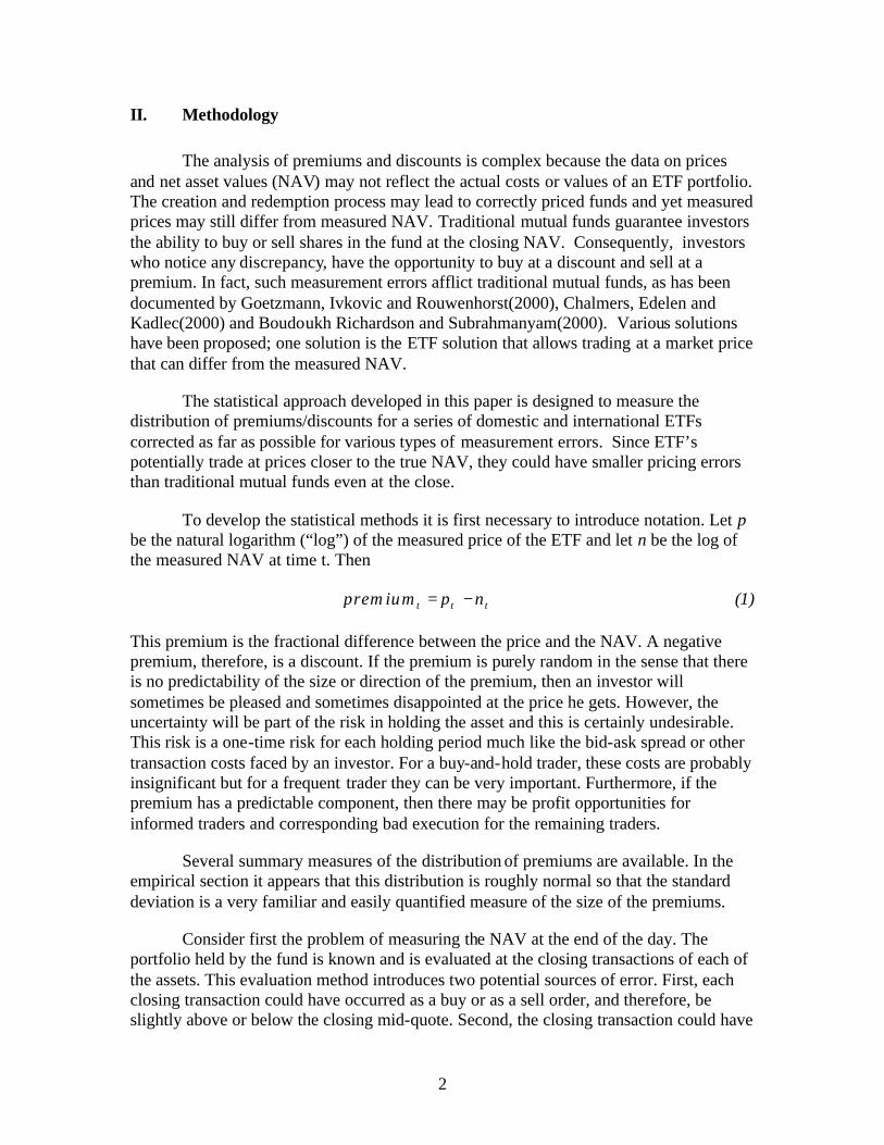
II. Methodology

The analysis of premiums and discounts is complex because the data on prices and net asset values (NAV) may not reflect the actual costs or values of an ETF portfolio. The creation and redemption process may lead to correctly priced funds and yet measured prices may still differ from measured NAV. Traditional mutual funds guarantee investors the ability to buy or sell shares in the fund at the closing NAV. Consequently, investors who notice any discrepancy, have the opportunity to buy at a discount and sell at a premium. In fact, such measurement errors afflict traditional mutual funds, as has been documented by Goetzmann, Ivkovic and Rouwenhorst(2000), Chalmers, Edelen and Kadlec(2000) and Boudoukh Richardson and Subrahmanyam(2000). Various solutions have been proposed; one solution is the ETF solution that allows trading at a market price that can differ from the measured NAV.

The statistical approach developed in this paper is designed to measure the distribution of premiums/discounts for a series of domestic and international ETFs corrected as far as possible for various types of measurement errors. Since ETF’s potentially trade at prices closer to the true NAV, they could have smaller pricing errors than traditional mutual funds even at the close.

To develop the statistical methods it is first necessary to introduce notation. Let p be the natural logarithm (“log”) of the measured price of the ETF and let n be the log of the measured NAV at time t. Then

t t tpremium p n= − (1)

This premium is the fractional difference between the price and the NAV. A negative premium, therefore, is a discount. If the premium is purely random in the sense that there is no predictability of the size or direction of the premium, then an investor will sometimes be pleased and sometimes disappointed at the price he gets. However, the uncertainty will be part of the risk in holding the asset and this is certainly undesirable. This risk is a one-time risk for each holding period much like the bid-ask spread or other transaction costs faced by an investor. For a buy-and-hold trader, these costs are probably insignificant but for a frequent trader they can be very important. Furthermore, if the premium has a predictable component, then there may be profit opportunities for informed traders and corresponding bad execution for the remaining traders.

Several summary measures of the distribution of premiums are available. In the empirical section it appears that this distribution is roughly normal so that the standard deviation is a very familiar and easily quantified measure of the size of the premiums.

Consider first the problem of measuring the NAV at the end of the day. The portfolio held by the fund is known and is evaluated at the closing transactions of each of the assets. This evaluation method introduces two potential sources of error. First, each closing transaction could have occurred as a buy or as a sell order, and therefore, be slightly above or below the closing mid-quote. Second, the closing transaction could have

3

occurred early in the day, particularly for infrequently traded stocks. As a result, the transaction may not contain information on its end of day value. An institutional investor considering creating or redeeming shares will compare the current value of these shares at the end of the day to the fund share price, and will trade regardless of the accounting definition of NAV.

The NAV is only calculated at the market close. Within the day, however, an estimated value of the portfolio is continually posted. This IOPV (Indicative Optimized Portfolio Value) is updated on a 15 second interval using the most recent transaction price of each component of the portfolio. Consequently, it will also have the same stale quote possibility as the NAV at the close.

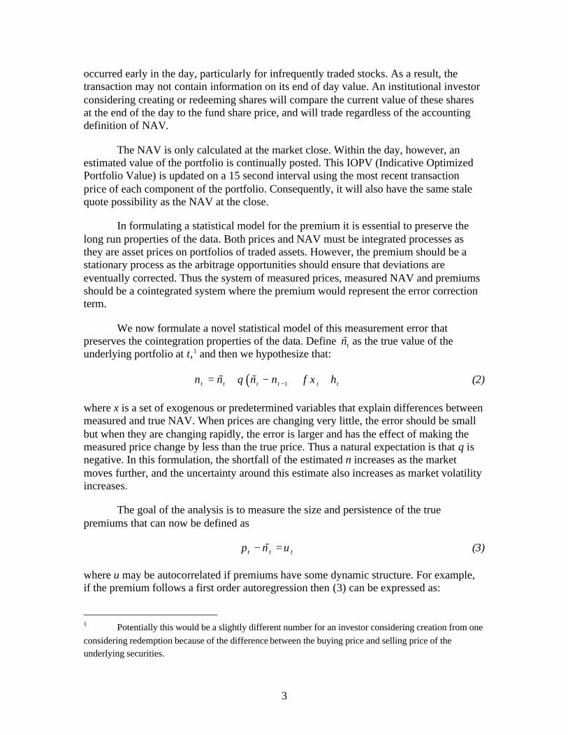
In formulating a statistical model for the premium it is essential to preserve the long run properties of the data. Both prices and NAV must be integrated processes as they are asset prices on portfolios of traded assets. However, the premium should be a stationary process as the arbitrage opportunities should ensure that deviations are eventually corrected. Thus the system of measured prices, measured NAV and premiums should be a cointegrated system where the premium would represent the error correction term.

We now formulate a novel statistical model of this measurement error that preserves the cointegration properties of the data. Define tn% as the true value of the underlying portfolio at t,1 and then we hypothesize that:

( )1t t t t t tn n n n xθ φ η−= + − + +% % (2)

where x is a set of exogenous or predetermined variables that explain differences between measured and true NAV. When prices are changing very little, the error should be small but when they are changing rapidly, the error is larger and has the effect of making the measured price change by less than the true price. Thus a natural expectation is that θ is negative. In this formulation, the shortfall of the estimated n increases as the market moves further, and the uncertainty around this estimate also increases as market volatility increases.

The goal of the analysis is to measure the size and persistence of the true premiums that can now be defined as

t t tp n u− =% (3)

where u may be autocorrelated if premiums have some dynamic structure. For example, if the premium follows a first order autoregression then (3) can be expressed as:

1 Potentially this would be a slightly different number for an investor considering creation from one considering redemption because of the difference between the buying price and selling price of the underlying securities.

4

( )1 1t t t t tp n p nρ ε− −− = − +% % (4)

Assume that the growth of NAV has a constant mean,

t tdn µ ξ= +% (5)

and assume that all three shocks are independent and normally distributed.2

The system of equations (2),(4),(5) can then be expressed in a state space framework and estimated with the Kalman Filter. See for example Harvey(1989) or Hamilton(1994).

1

1 2

1

1 1

1 01 0 0 0

11 0

t t t

t t

t t t t

t t t t t

n nn n

p p nn n x n

µ ξ

ρ ερθ φ ηθ

−

− −

−

− −

= + +

−

= + + − + +

% %% %

%%

(6)

The Kalman filter will provide forecasts of the true NAV and true premium based on past information. These estimates can be further refined based on subsequent data to estimate what the true NAV was at any time. The parameters of this system can be estimated by maximizing the likelihood with respect to the unknown variances and mean parameters. The standard deviation of the innovation to the true premium, ε is related to the standard deviation of u by

21

uεσ

σρ

=−

(7)

The methodology however is greatly simplified if it turns out that the errors in the NAV equation (2) are small relative to the others. This would generally be expected, since the magnitude of the stale quote error is likely to be smaller than the rate of change of the price or the deviation of the premium. Assuming that (2) has no error term, it can be solved with equation (3) to eliminate the unobserved true NAV.

( )11 1t t t t t t

t t t

p n n n x u

n x u

θ φθ θ

α β

−− = − − − ++ +

≡ ∆ + +

(8)

If the first order autoregressive assumption is sufficient for the premiums, then equation (8) will simply require an AR(1) error specification. The unconditional standard deviation

2 The normality assumption can be weakened when the Kalman Filter is interpreted as the linear projection rather than the conditional distribution.

5

is estimated by the standard deviation of { }t̂u . Notice that this model is consistent with the cointegration hypothesis since all variables on both sides of the equation are stationary. Because θ is negative, the coefficient α should be positive. This means that rapid increases in NAV should result in especially large premiums because the measured NAV will be an underestimate of the true NAV.

If the variance of the measurement error in (2) is not zero, then (8) will only be an approximation. The disturbance in the equation will become

( )/ 1t tu η θ− + (9)

This additional term has several implications. Because η is correlated with tn∆ , the least squares coefficient estimates will be biased and inconsistent. The estimate of α will be downward biased and likely negative. Thus large increases in NAV will be associated with reduced premiums since part of the increase in NAV is attributed to measurement error. The standard deviation of (9) will exceed the standard deviation of u, but the least squares estimate will be less biased since some of the variability of η will be attributed to

tn∆ . The composite error term in (9) will have more complex time series structure. For example, if u is an AR(1), then the composite error will be an ARMA(1,1). Thus, for small measurement errors, the standard deviation of the autoregressive error will be a conservative estimate of the true premium standard deviation. If the measurement errors are more significant than this, then the model in (6) must be used. Some examples will be presented to show the relation between these two estimates.

In some markets, it is possible to improve the measurement of n using futures prices. Since the futures are priced as:

( )r q Tt tF S e −= (10)

with T as the remaining time to expiration of the futures contract and q as the continuous dividend yield, a futures price implicitly estimates the cash price just by resolving this equation. To incorporate this into the measurement equation for NAV, define

( ) ( )logt t tA F r q T n= − − − (11)

Then equation (2) becomes

( )1t t t t t tn n n n Aθ φ η−= + − + +% % (12)

where one might anticipate a value of 1φ = − .

Further measurement errors are introduced through the timing of market closing. For many of the ETFs the market closes at 4:15 Eastern Time while the NAV is calculated at 4:00, when the equity markets close. As a consequence, in daily data there is another important measurement error in the NAV. Calculation of the 4:15 NAV for funds with futures contracts simply requires the change in the futures price between the close of

6

the two markets. Calling this post market change in futures, Fpm, equation (12) now can be written as,

( )1t t t t t t tn n n n A Fpmθ φ β η−= + − + + +% % (13)

and the premium equation (8) becomes:

( )1 1 2t t t t t t tp n n n A Fpm uα β β−− = − + + + (14)

Allowing for an autoregressive error structure as in (4), the estimating equation is

( ) ( ) ( ) ( )1 1 1 1 1 2 1t t t t t t t t t t tp n p n n n A A Fpm Fpmρ α ρ β ρ β ρ ε− − − − −− = − + ∆ − ∆ + − + − + (15)

which will be referred to as the dyna model. The regression of spread, therefore, includes the change in NAV, the future returns from 4:00pm to 4:15pm and the futures based cash adjustment. For some ETFs only a subset of these variables will be available or relevant.

Serial correlation corrections will be needed if there remains autocorrelation in the premium. The unconditional error in the premium can be directly calculated from (15) by examining the sum of squared residuals of (14) using the coefficients estimated in (15). The coefficients are estimated more efficiently in (15) but the residuals measure only the unpredictable portion of the premium, not the entire premium. When these differ, it is the entire premium that reflects the importance of premiums and discounts. While there may still be errors in the premium due to noisy measurement of p due to bid-ask spread or staleness, these price effects can be almost eliminated by using closing mid-quotes rather than last trade prices.3

Once the effects of the independent variables are taken out, the residuals reflect the remaining premium and discount. Thus, the standard deviation of the residuals is a good measure of the size of the pricing errors that actually occur. If the residual variance changes over time, as it is likely to do from the model presented above, heteroskedasticity corrections can measure when it is large and when it is small.

In each of these models, the error variance is reasonably assumed to be proportional to the volatility of the underlying asset. To model this, a heteroskedasticity correction can be used. Suppose the residual variance is modeled as

2 exp( )t tzσ δ= (16)

3 In fact, we will show later that the standard deviation of mid-quote premium regression is smaller than that of transaction premium regression.

7

where z reflects a vector of variables measuring the volatility of the underlying asset. The simplest version takes ' (log( / ), )t t tz high low c= where c is an intercept. A more flexible model sets:

( ) ( )2 21 1exp( ), 1 exp 2t t t t t t th z h a b ae z bhσ δ δ− −= = − − + − + (17)

where e are the residuals from the model. With either of these formulations of the heteroskedasticity, the model is estimated by maximum likelihood with a conventional conditional Gaussian likelihood function given by

2

22

1 log( )2

tt

t t

eL σσ

= − +

∑ (18)

III. Preliminary Results

To examine the performance of these models on several different series, we consider three end-of-day data sets, DIA, XLK, and EWA. These ETFs are based respectively on the Dow Jones Industrials, S&P Technology Sector and MSCI Australia index, and the closing prices are measured as the midpoint of the closing bid and ask quotes.

These three series have very different problems. The DIA trades until 4:15, while the XLK closes at 4:00. There is a futures contract traded on the Dow until 4:15 that can be used to correct the NAV both for stale quotes and for the timing discrepancies. There is no futures contract on XLK although it is possible that its staleness would be related to the same measure for a broad market index, such as S&P 500. Although the EWA closes at 4:00, it trades entirely while the underlying market (Australia) is closed so it could be considered to have a very stale value for NAV. The recorded value of NAV in this case is simply the closing price of the basket in Australia, adjusted for changes in currency values until 4:00 Eastern Time.

In each case, the objective is to determine the size and persistence of the premiums. Plots of the premiums are shown in Figures 1 and 2. As can be seen, they have substantial variability but little obvious predictability, particularly for the domestic funds. There is substantial evidence that the variability of the premium changes over time. In Figures 3 and 4, histograms of XLF at the end of the day and IWM on a 1 minute intra-daily basis are presented. These show that the distribution of these premiums and discounts is roughly shaped like the normal bell curve. As a result, the size of the premiums can be conveniently assessed by the standard deviation even though there are more extremes than one would expect under the normality assumption. This measure is formulated in basis points and can easily be compared with other costs such as bid-ask spreads or commissions. The dynamic properties of the premiums can be assessed by examination of the autocorrelations of the data and decay rates as will be presented below.

8

The first panel of Table 1 gives the standard deviations of last trade-based premium and midquote-based premium. Both are expressed in percent. For example, the standard deviation of the DIA closing premium using last trade prices is 0.22% or 22 basis points. The same measure using the midquote is only 20 bps. The use of the midquote reduces the standard deviation for each of these products and in fact for all the products, particularly the less actively traded products such as XLK and EWA. The midquote standard deviation of XLK and EWA are 16 bps and 86 bps respectively.

The regression results for these three series based on equation (14) are given in the second panel of Table 1. The DIA has a very large and significant effect from the futures price change from 4:00 to 4:15. This number is again in percent so that the correction to the NAV is estimated to be 70% of the change in the futures price. The adjustment to the estimated cash value at 4:00 is estimated to be only 10% of the prediction based on the futures price. The change in the NAV from one day to the next is found to be significantly positive, in accordance with the formulation of equation (2). Rising NAV implies that the measured NAV is too low because some quotes will be stale and consequently, the premium is too high. The autocorrelation in the errors is estimated to be 0.13, which is quite small. Therefore, the estimated standard deviation of the true premium is just the standard deviation of the regression or 11.7 bps. The mean premium is 4 basis points. The adjustments to NAV based on the futures prices, correcting for the timing discrepancy and for the estimated cash value, are effective in bringing the standard deviation from 20 bps to 11.7 bps, down by almost half.

For the XLK, there is no timing mismatch and no futures contract. Hence the cash adjustment for the S&P500 futures is used in the regression. This, however, is not significant. The change in NAV is significant, but now it has the sign associated with errors-in-variables; increasing NAV reduces the premium; that is, the premium is now measured relative to an overstated estimate of NAV. While the stale quote feature may still be important, it is dominated by the measurement error in NAV. There remains little serial correlation, and the final estimate of the standard deviation of the premium is 15 bps. Notice that this is now higher than the DIA, which is expected due to the reduced transaction volume and narrower sector coverage. The mean premium is about 2 basis points.

The Australia index has no US traded futures contract and therefore is priced only by reference to the measured NAV. The coefficient on the change in NAV is significantly negative reinforcing the prior expectation that this will be strongly measured with error. The autocorrelation is estimated to be very significant at 0.36. The standard deviation of the true premium is calculated by simply ignoring the autocorrelation and is, therefore, noticeably bigger than the standard deviation of the regression and, in fact, slightly larger than the unconditional standard deviation. This reflects the finding that only a small part of the premium can be attributed to the hypothesized forms of measurement error. The mean premium is now noticeably positive at 47 basis points. The finding of a large positive mean premium is characteristic of the international ETFs and will be discussed later.

9

For two of these series, there is evidence that the measurement errors on the NAV are important in that changes negatively affect the premium. Therefore it may be important to estimate the Kalman Filter version of the model given in equation (6). This estimation procedure relies on identifying the measurement errors in NAV and the premium separately from the time series data. The results are given in the third panel of Table 1. For the first two indices, the measurement error standard deviation is much smaller than the premium standard deviation and the premium autocorrelation, measured by rho, is nearly zero. Hence, the model gives practically the same estimated standard deviation as the least squares model. However, for the EWA, the standard deviation of the NAV is much bigger and there is autocorrelation of 0.92 in the premium. From equation (7), this is 0.49 or 49 bps. This suggests a substantially better performance of the index. This model attributes much of the measured premium to errors in the NAV. However, the true premium now is found to have more autocorrelation. The estimates given by the dyna model are conservative as argued in the development of the model.

The volatility of the premium is not necessarily constant. In fact, visual inspection and statistical tests both indicate that it is changing over time. In the last panel of Table 1, equation (15) is estimated with heteroskedasticity correction given by (17). While the parameter values are rather similar to those in the upper panels, the graphs of conditional variance are quite interesting. In Figure 1, the standard deviation of the DIA premi um is graphed from the basic model with no adjustment for measurement errors in NAV and from the dyna model. The time variation in the standard deviation is partly a result of variation in the volatility of the Dow itself as measured by the daily high/low ratio. It also is due in part to persistent swings in standard deviations that are modeled by GARCH. The reduction in standard deviation is more or less uniform across time, but is particularly effective at times when the standard deviations are greatest.

The standard deviation estimator for the XLK is plotted with the premium itself in Figure 2. On the graph ± 2 standard deviations form an approximate 95% confidence interval. Clearly this is highly variable but pretty reliable as an indicator of the possible movements. In Figure 3, the standard deviation of the Australian ETF is plotted. The scale on this plot is noticeably greater with some periods having a standard deviation greater than 2%.

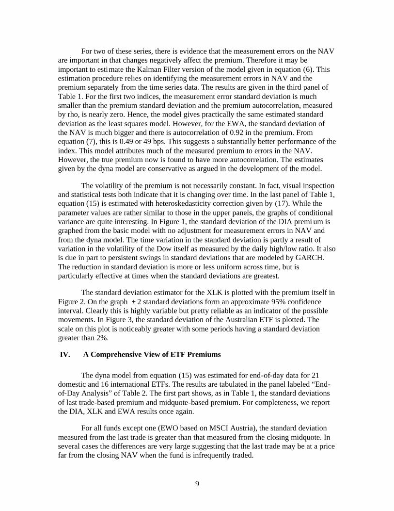
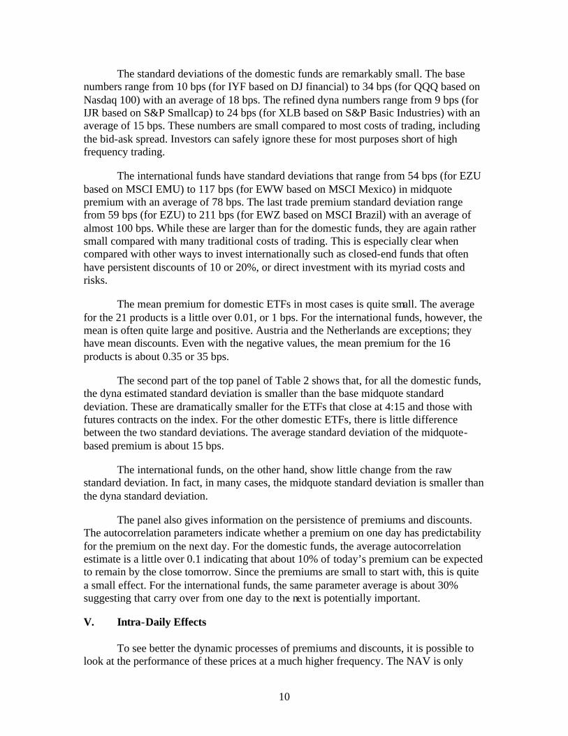
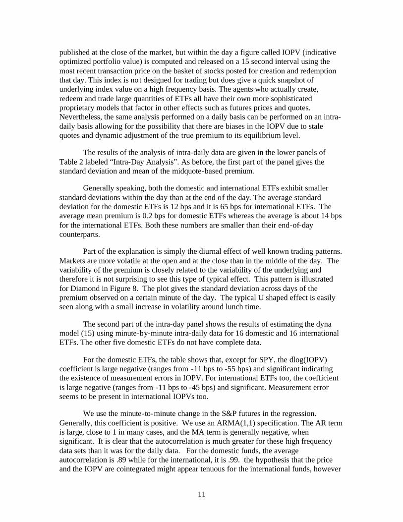
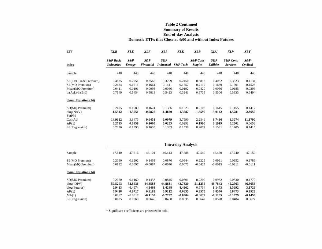
IV. A Comprehensive View of ETF Premiums

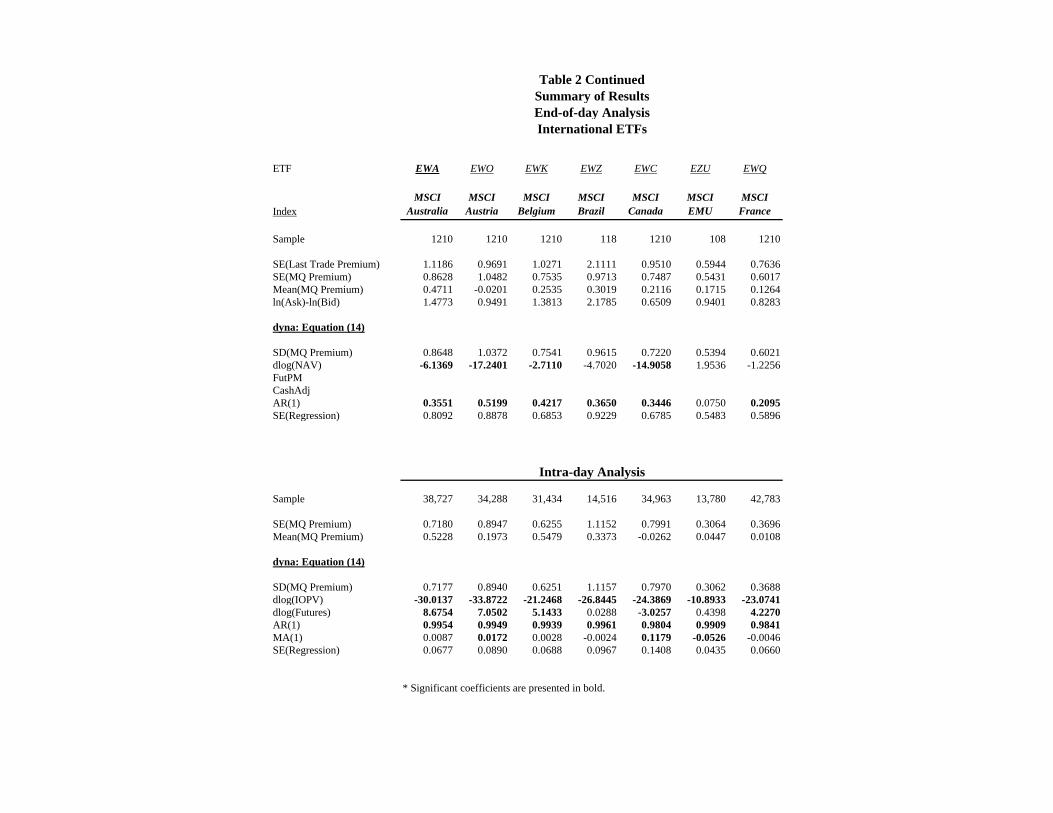
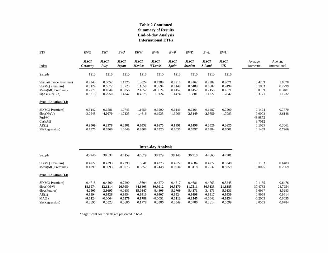
The dyna model from equation (15) was estimated for end-of-day data for 21 domestic and 16 international ETFs. The results are tabulated in the panel labeled “End-of-Day Analysis” of Table 2. The first part shows, as in Table 1, the standard deviations of last trade-based premium and midquote-based premium. For completeness, we report the DIA, XLK and EWA results once again.

For all funds except one (EWO based on MSCI Austria), the standard deviation measured from the last trade is greater than that measured from the closing midquote. In several cases the differences are very large suggesting that the last trade may be at a price far from the closing NAV when the fund is infrequently traded.

10

The standard deviations of the domestic funds are remarkably small. The base numbers range from 10 bps (for IYF based on DJ financial) to 34 bps (for QQQ based on Nasdaq 100) with an average of 18 bps. The refined dyna numbers range from 9 bps (for IJR based on S&P Smallcap) to 24 bps (for XLB based on S&P Basic Industries) with an average of 15 bps. These numbers are small compared to most costs of trading, including the bid-ask spread. Investors can safely ignore these for most purposes short of high frequency trading.

The international funds have standard deviations that range from 54 bps (for EZU based on MSCI EMU) to 117 bps (for EWW based on MSCI Mexico) in midquote premium with an average of 78 bps. The last trade premium standard deviation range from 59 bps (for EZU) to 211 bps (for EWZ based on MSCI Brazil) with an average of almost 100 bps. While these are larger than for the domestic funds, they are again rather small compared with many traditional costs of trading. This is especially clear when compared with other ways to invest internationally such as closed-end funds that often have persistent discounts of 10 or 20%, or direct investment with its myriad costs and risks.

The mean premium for domestic ETFs in most cases is quite small. The average for the 21 products is a little over 0.01, or 1 bps. For the international funds, however, the mean is often quite large and positive. Austria and the Netherlands are exceptions; they have mean discounts. Even with the negative values, the mean premium for the 16 products is about 0.35 or 35 bps.

The second part of the top panel of Table 2 shows that, for all the domestic funds, the dyna estimated standard deviation is smaller than the base midquote standard deviation. These are dramatically smaller for the ETFs that close at 4:15 and those with futures contracts on the index. For the other domestic ETFs, there is little difference between the two standard deviations. The average standard deviation of the midquote-based premium is about 15 bps.

The international funds, on the other hand, show little change from the raw standard deviation. In fact, in many cases, the midquote standard deviation is smaller than the dyna standard deviation.

The panel also gives information on the persistence of premiums and discounts. The autocorrelation parameters indicate whether a premium on one day has predictability for the premium on the next day. For the domestic funds, the average autocorrelation estimate is a little over 0.1 indicating that about 10% of today’s premium can be expected to remain by the close tomorrow. Since the premiums are small to start with, this is quite a small effect. For the international funds, the same parameter average is about 30% suggesting that carry over from one day to the next is potentially important.

V. Intra-Daily Effects To see better the dynamic processes of premiums and discounts, it is possible to

look at the performance of these prices at a much higher frequency. The NAV is only

11

published at the close of the market, but within the day a figure called IOPV (indicative optimized portfolio value) is computed and released on a 15 second interval using the most recent transaction price on the basket of stocks posted for creation and redemption that day. This index is not designed for trading but does give a quick snapshot of underlying index value on a high frequency basis. The agents who actually create, redeem and trade large quantities of ETFs all have their own more sophisticated proprietary models that factor in other effects such as futures prices and quotes. Nevertheless, the same analysis performed on a daily basis can be performed on an intra-daily basis allowing for the possibility that there are biases in the IOPV due to stale quotes and dynamic adjustment of the true premium to its equilibrium level.

The results of the analysis of intra-daily data are given in the lower panels of Table 2 labeled “Intra-Day Analysis”. As before, the first part of the panel gives the standard deviation and mean of the midquote-based premium.

Generally speaking, both the domestic and international ETFs exhibit smaller standard deviations within the day than at the end of the day. The average standard deviation for the domestic ETFs is 12 bps and it is 65 bps for international ETFs. The average mean premium is 0.2 bps for domestic ETFs whereas the average is about 14 bps for the international ETFs. Both these numbers are smaller than their end-of-day counterparts.

Part of the explanation is simply the diurnal effect of well known trading patterns. Markets are more volatile at the open and at the close than in the middle of the day. The variability of the premium is closely related to the variability of the underlying and therefore it is not surprising to see this type of typical effect. This pattern is illustrated for Diamond in Figure 8. The plot gives the standard deviation across days of the premium observed on a certain minute of the day. The typical U shaped effect is easily seen along with a small increase in volatility around lunch time.

The second part of the intra-day panel shows the results of estimating the dyna model (15) using minute-by-minute intra-daily data for 16 domestic and 16 international ETFs. The other five domestic ETFs do not have complete data.

For the domestic ETFs, the table shows that, except for SPY, the dlog(IOPV) coefficient is large negative (ranges from -11 bps to -55 bps) and significant indicating the existence of measurement errors in IOPV. For international ETFs too, the coefficient is large negative (ranges from -11 bps to -45 bps) and significant. Measurement error seems to be present in international IOPVs too.

We use the minute-to-minute change in the S&P futures in the regression. Generally, this coefficient is positive. We use an ARMA(1,1) specification. The AR term is large, close to 1 in many cases, and the MA term is generally negative, when significant. It is clear that the autocorrelation is much greater for these high frequency data sets than it was for the daily data. For the domestic funds, the average autocorrelation is .89 while for the international, it is .99. the hypothesis that the price and the IOPV are cointegrated might appear tenuous for the international funds, however

12

a direct test concludes that these series are cointegrated in every case. While there is some explanatory power in the regressors introduced into these regressions, the estimated standard deviation of the premium is reduced imperceptibly in almost all cases.

The lengths of the lags can be examined in more detail with these high frequency data. We calculate the length of time that a large premium takes to revert to the mean value. For each asset we define an upper and a lower threshold. We measure the duration of a large premium starting when it first exceeds the upper threshold and continuing until it first crosses the lower threshold. This is done separately for premiums and discounts. These durations are presented in Table 3.

From these results it is clear that the typical large duration episode lasts only a few minutes for the majority of the domestic funds. For the Spiders and Diamonds, the median duration is 5 to 7 minutes. On average over all domestic funds it is 10 minutes and the distribution is more or less symmetric between premium events and discount events. For the international funds, the typical premium event lasts 177 minutes while for discounts it is 169 minutes. These numbers are much larger – almost 3 hours. The mean durations are longer still as the distribution is highly skewed. The average duration is about 5 hours with many lasting several days.

One reason these episodes last so long, is the infrequency of trades and quote revisions for the international funds. In Table 4, it can be seen that trades occur on average about every 30 minutes and quotes are revised less frequently, sometimes more than 2 hours apart on average. This sluggish response to information is only consistent with the absence of arbitrage when the spreads are large. This is indeed the case with these international funds.

The story of the international fund pricing is that the prices move slowly in response to economic news, but that spreads are apparently wide enough to prevent arbitrage. How wide are the spreads? These are tabulated in Table 2. Domestically, the end of day average spread over funds is 37 basis points, although this is dominated by a few of the sector funds. The broad indices have spreads under 20 basis points. The international funds have spreads that average 112 bps.

Although these spreads are large, in the context of international investment vehicles, they are not. The are small compared to the persistent premiums of closed end country funds and are smaller than one typically finds for ADR’s and other international replication instruments.

V. Conclusions

This study has examined the magnitude of premiums and discounts for a wide range of Exchange Traded Funds. These include domestic funds with and without

13

futures contracts, and closing at 4:00 or 4:15. These include broad market indices and narrow sector funds. The sector funds range from utilities and basic industries to technology and internet sectors. In almost all cases, the mean premium was less than 5 bps and the standard deviation was less than 20 bps.

We develop a statistical approach to measuring the true premium by correcting some of the measurement errors in net asset value. This reduces further the observed standard deviation. We examine how the standard deviation moves over time. The resulting standard deviation of the premium is 9bps for some funds and averages 14. For the international funds the estimate of the standard deviation averages 77 bps.

From a minute-by-minute point of view, the standard deviations are even smaller. It now becomes possible to see how long episodes of premium or discount last. The domestic episodes generally last only a few minutes with an average across funds of 10 minutes. The international funds last typically almost 3 hours with some even slower to recover.

The overall impression of the domestic funds is of a set of products that are priced very close to their market value with only brief excursions any distance away. The international funds are less actively traded and less precisely priced; yet they operate in a more stringent environment and may still be performing according to expectations.

14

REFERENCES

Boudoukh, Jacob, Matthew Richardson and Marti Subrahmanyam,(2000) “The Last Great Arbitrage: Exploiting the Buy-and-Hold Mutual Fund Investor” , NYU Working Paper. Chalmers, John, Roger Edelen and Gregory Kadlec (2001) “On the Perils of Financial Intermediaries Setting Security Prices: The Mutual Fund Wild Card Option”, The Journal of Finance, vol. 56, no. 6, pp. 2209-2236. Goetzmann, William, Zoran Ivkovic and Geert Rouwenhorst (2001) “Day Trading International Mutual Funds: Evidence and Policy Solutions,” Journal of Financial and Quantitative Analysis, vol. 36, no. 3. Harvey, A.C. (1989), Forecasting, Structural Time Series Models, and the Kalman Filter, Cambridge University Press. Hamilton, J.D. (1994), Time Series Analysis, Princeton University Press.

Table 1

Results for Three ETFs: End-of-Day Analysis

DIA XLK EWAIndex Dow Jones S&P Tech AustraliaSample 682 448 1210

SE(Last Trade Premium) 0.2165 0.2450 1.1186SE(MidQuote Premium) 0.2018 0.1557 0.8628

dyna: Equation (14)

SD(MidQuote Premium) 0.1175 0.1523 0.8648Intercept -0.0424 -0.0311 0.4719dlog(NAV) 2.5885 -1.3587 -6.1369FutPM 69.7065CashAdj 10.4748 3.7590AR(1) 0.1253 0.0291 0.3551SE(Regression) 0.1171 0.1530 0.8092

State Space: Equation (6)rho 9.91E-06 -1.83E-05 0.9226theta -0.0280 0.0142 -0.2835FutPM -65.5649CashAdj -8.7155 -4.3768SD(True Premium) 0.1162 0.1543 0.1873SD(Measurement Error) 0.0192 0.0210 0.6146

GARCH rho 0.1484 0.0609 0.4083dlog(NAV) 2.0809 -1.7070 -5.9001FutPM 71.2333CashAdj 9.6440 3.5434Intercept -0.0328 -0.0231 0.2586VarianceHiLo 41.7061 36.5452 37.7495ARCH 0.0336 0.0585 0.0694

* Significant coefficients are presented in bold.

Table 2Summary of ResultsEnd-of-day Analysis

Domestic ETFs that Close at 4:15: Grouped by Those with Index Futures and Those without

ETF DIA IJH IVV IWB IWM MDY QQQ SPY IJR IYF IYV IYW

Index DJIAS&P

Midcap S&P 500Russell 1000

Russell 2000

S&P Midcap

Nasdaq 100 S&P 500

S&P Smallcap

DJ Financial

DJ Internet DJ Tech

Sample 682 88 93 93 88 1365 396 946 88 88 93

SE(Last Trade Premium) 0.2165 0.3036 0.1758 0.4675 0.2821 0.3525 0.3896 0.2262 0.3995 0.4103 1.4198 0.8854SE(MQ Premium) 0.2018 0.1577 0.1673 0.1684 0.2446 0.2853 0.3395 0.2141 0.1501 0.1008 0.1069 0.1565Mean(MQ Premium) 0.0456 0.0222 0.0318 0.0297 -0.0095 0.0285 0.0079 0.0026 0.0250 -0.0075 0.0382 -0.0200ln(Ask)-ln(Bid) 0.1674 0.1770 0.0827 0.1662 0.2997 0.2202 0.1674 0.0826 0.1514 0.3499 0.4409 0.3681

dyna: Equation (14)

SD(MQ Premium) 0.1175 0.1405 0.0889 0.1014 0.1672 0.2234 0.1984 0.1008 0.0928 0.0968 0.1024 0.1525dlog(NAV) 2.5885 2.7690 -2.3650 -3.4844 8.4666 6.1950 1.0761 2.5410 0.7516 -1.4016 -0.3532 -0.8815FutPM 69.7065 40.1233 83.1178 76.2597 20.4763 40.1806 66.4744 78.3499 76.8738 -6.9733 -19.5102 2.7679CashAdj 10.4748 1.6663 7.1689 6.2809 21.1365 20.7773 21.5105 15.7105 2.9680 2.0423 3.2273 1.0562AR(1) 0.1253 0.1538 0.1089 0.1556 0.0729 0.1188 0.1772 0.1253 -0.0672 0.2597 -0.0097 -0.3008SE(Regression) 0.1171 0.1436 0.0911 0.1035 0.1720 0.2224 0.1965 0.1003 0.0953 0.0954 0.1048 0.1505

Intra-day Analysis

Sample 45,239 32,503 35,864 33,072 46,673 47,506 47,446

SE(MQ Premium) 0.0715 0.0690 0.0788 0.1275 0.1189 0.1272 0.0690Mean(MQ Premium) -0.0079 0.0257 0.0135 0.0140 0.0250 0.0129 0.0133

dyna: Equation (14)

SD(MQ Premium) 0.0713 0.0690 0.0783 0.1282 0.1178 0.1261 0.0669dlog(IOPV) -10.2319 -35.7536 -10.9811 -50.2754 -55.0938 -13.2941 3.9793dlog(Futures) 9.4701 1.7110 17.3190 5.3920 5.1205 12.7447 16.1715AR(1) 0.8798 0.9333 0.9747 0.9518 0.9171 0.8444 0.9274MA(1) -0.3149 -0.3392 -0.6385 -0.0297 -0.0597 -0.3970 -0.5775SE(Regression) 0.0459 0.0358 0.0434 0.0405 0.0496 0.0968 0.0489

* Significant coefficients are presented in bold.

ETF

Index

Sample

SE(Last Trade Premium)SE(MQ Premium)Mean(MQ Premium)ln(Ask)-ln(Bid)

dyna: Equation (14)

SD(MQ Premium)dlog(NAV)FutPMCashAdjAR(1)SE(Regression)

Sample

SE(MQ Premium)Mean(MQ Premium)

dyna: Equation (14)

SD(MQ Premium)dlog(IOPV)dlog(Futures)AR(1)MA(1)SE(Regression)

Table 2 ContinuedSummary of ResultsEnd-of-day Analysis

Domestic ETFs that Close at 4:00 and without Index Futures

XLB XLE XLF XLI XLK XLP XLU XLV XLY

S&P Basic Industries

S&P Energy

S&P Financial

S&P Industrial S&P Tech

S&P Cons Staples

S&P Utilities

S&P Cons Services

S&P Cyclical

448 448 448 448 448 448 448 448 448

0.4835 0.2951 0.3565 0.3799 0.2450 0.3818 0.4032 0.3523 0.41340.2484 0.1611 0.1664 0.1411 0.1557 0.2119 0.1689 0.1501 0.15280.0411 0.0101 -0.0098 0.0046 0.0192 -0.0420 0.0086 -0.0185 0.02030.7949 0.5454 0.5813 0.5423 0.3241 0.6739 0.5506 0.5833 0.6494

0.2405 0.1589 0.1624 0.1386 0.1523 0.2108 0.1615 0.1455 0.1417-1.5942 -1.3751 -0.9827 -1.4660 -1.3587 -1.6599 -3.0142 -1.5781 -2.8659

14.9622 3.8475 9.6451 6.0079 3.7590 2.2546 8.7436 8.3074 11.17900.2735 0.0958 0.1660 0.0253 0.0291 0.1990 0.1919 0.2501 0.06580.2326 0.1590 0.1605 0.1393 0.1530 0.2077 0.1591 0.1405 0.1415

Intra-day Analysis

47,610 47,616 46,104 46,413 47,588 47,540 46,450 47,740 47,159

0.2080 0.1202 0.1468 0.0876 0.0844 0.2225 0.0981 0.0852 0.17860.0192 0.0097 -0.0087 -0.0070 0.0072 -0.0425 -0.0015 -0.0211 -0.0111

0.2050 0.1160 0.1458 0.0845 0.0801 0.2209 0.0932 0.0830 0.1770-50.5203 -52.8636 -44.3588 -44.8631 -43.7830 -51.1256 -48.7843 -45.2563 -46.3656

0.9423 -0.4074 4.3469 1.4248 8.4962 0.5754 1.1473 3.5692 3.17260.9418 0.8717 0.9182 0.9112 0.6635 0.9575 0.8576 0.8473 0.95230.0067 -0.0017 -0.1158 -0.2752 -0.0904 -0.0074 -0.1105 -0.1079 -0.14590.0685 0.0569 0.0646 0.0460 0.0635 0.0642 0.0528 0.0484 0.0627

* Significant coefficients are presented in bold.

ETF

Index

Sample

SE(Last Trade Premium)SE(MQ Premium)Mean(MQ Premium)ln(Ask)-ln(Bid)

dyna: Equation (14)

SD(MQ Premium)dlog(NAV)FutPMCashAdjAR(1)SE(Regression)

Sample

SE(MQ Premium)Mean(MQ Premium)

dyna: Equation (14)

SD(MQ Premium)dlog(IOPV)dlog(Futures)AR(1)MA(1)SE(Regression)

Table 2 ContinuedSummary of ResultsEnd-of-day AnalysisInternational ETFs

EWA EWO EWK EWZ EWC EZU EWQ

MSCI Australia

MSCI Austria

MSCI Belgium

MSCI Brazil

MSCI Canada

MSCI EMU

MSCI France

1210 1210 1210 118 1210 108 1210

1.1186 0.9691 1.0271 2.1111 0.9510 0.5944 0.76360.8628 1.0482 0.7535 0.9713 0.7487 0.5431 0.60170.4711 -0.0201 0.2535 0.3019 0.2116 0.1715 0.12641.4773 0.9491 1.3813 2.1785 0.6509 0.9401 0.8283

0.8648 1.0372 0.7541 0.9615 0.7220 0.5394 0.6021-6.1369 -17.2401 -2.7110 -4.7020 -14.9058 1.9536 -1.2256

0.3551 0.5199 0.4217 0.3650 0.3446 0.0750 0.20950.8092 0.8878 0.6853 0.9229 0.6785 0.5483 0.5896

Intra-day Analysis

38,727 34,288 31,434 14,516 34,963 13,780 42,783

0.7180 0.8947 0.6255 1.1152 0.7991 0.3064 0.36960.5228 0.1973 0.5479 0.3373 -0.0262 0.0447 0.0108

0.7177 0.8940 0.6251 1.1157 0.7970 0.3062 0.3688-30.0137 -33.8722 -21.2468 -26.8445 -24.3869 -10.8933 -23.0741

8.6754 7.0502 5.1433 0.0288 -3.0257 0.4398 4.22700.9954 0.9949 0.9939 0.9961 0.9804 0.9909 0.98410.0087 0.0172 0.0028 -0.0024 0.1179 -0.0526 -0.00460.0677 0.0890 0.0688 0.0967 0.1408 0.0435 0.0660

* Significant coefficients are presented in bold.

ETF

Index

Sample

SE(Last Trade Premium)SE(MQ Premium)Mean(MQ Premium)ln(Ask)-ln(Bid)

dyna: Equation (14)

SD(MQ Premium)dlog(NAV)FutPMCashAdjAR(1)SE(Regression)

Sample

SE(MQ Premium)Mean(MQ Premium)

dyna: Equation (14)

SD(MQ Premium)dlog(IOPV)dlog(Futures)AR(1)MA(1)SE(Regression)

Table 2 ContinuedSummary of ResultsEnd-of-day AnalysisInternational ETFs

EWG EWI EWJ EWW EWN EWP EWD EWL EWU

MSCI Germany

MSCI Italy

MSCI Japan

MSCI Mexico

MSCI N'Lands

MSCI Spain

MSCI Sweden

MSCI S'Land

MSCI UK

Average Domestic

Average International

1210 1210 1210 1210 1210 1210 1210 1210 1210

0.9243 0.8052 1.1575 1.3824 0.7389 0.8210 0.9162 0.9382 0.9071 0.4209 1.00780.8124 0.6572 1.0720 1.1659 0.5594 0.6149 0.6489 0.6687 0.7494 0.1833 0.77990.2770 0.1044 0.3056 2.1852 -0.0624 0.4157 0.1452 0.2158 0.4671 0.0109 0.34810.9215 0.7950 1.4342 0.4575 1.0124 1.1474 1.3801 1.1327 1.2847 0.3771 1.1232

0.8142 0.6581 1.0745 1.1659 0.5590 0.6149 0.6464 0.6687 0.7500 0.1474 0.7770-2.2248 -4.0070 -1.7125 -1.4616 0.1925 -1.3966 2.5149 -2.9750 -1.7983 0.0003 -3.6148

43.98728.7012

0.2069 0.2578 0.3581 0.6032 0.1675 0.1991 0.1496 0.3026 0.3625 0.1055 0.30610.7975 0.6369 1.0049 0.9309 0.5520 0.6035 0.6397 0.6384 0.7001 0.1469 0.7266

Intra-day Analysis

45,946 38,534 47,159 42,679 38,279 39,140 36,910 44,665 44,981

0.4722 0.4293 0.7290 1.5641 0.4275 0.4522 0.4684 0.4772 0.5248 0.1183 0.64830.1099 0.0093 -0.0075 0.5352 0.2448 0.0934 0.0418 0.2537 0.8759 0.0025 0.2369

0.4718 0.4290 0.7290 1.5604 0.4270 0.4517 0.4681 0.4763 0.5245 0.1165 0.6476-18.6974 -13.1314 -26.9954 -44.6403 -30.9912 -20.5170 -11.7511 -36.9133 -21.6385 -37.4732 -24.7254

4.2505 2.9695 -0.0155 15.0147 8.4906 5.2769 5.4271 3.4873 5.0133 5.6997 4.52830.9894 0.9926 0.9954 0.9910 0.9907 0.9924 0.9898 0.9917 0.9939 0.8968 0.9914

-0.0124 -0.0064 0.0276 0.1788 -0.0051 0.0112 -0.1545 -0.0042 -0.0334 -0.2003 0.00550.0695 0.0523 0.0686 0.1778 0.0586 0.0549 0.0786 0.0614 0.0599 0.0555 0.0784

* Significant coefficients are presented in bold.

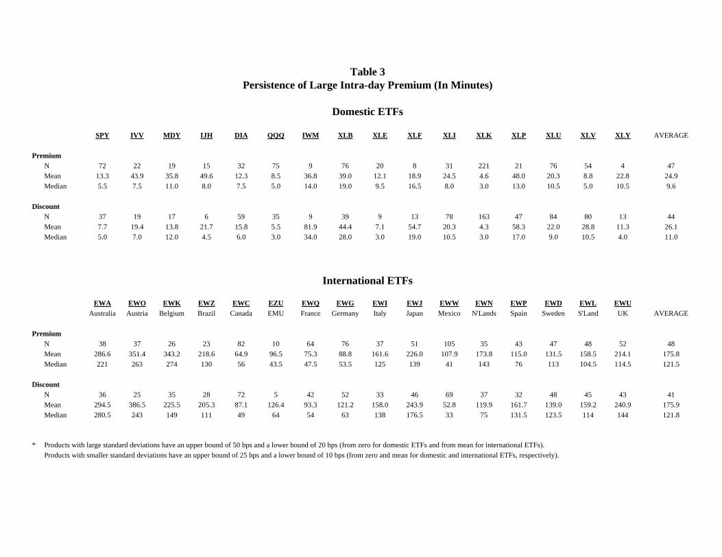
Table 3Persistence of Large Intra-day Premium (In Minutes)

Domestic ETFs

SPY IVV MDY IJH DIA QQQ IWM XLB XLE XLF XLI XLK XLP XLU XLV XLY AVERAGE

PremiumN 72 22 19 15 32 75 9 76 20 8 31 221 21 76 54 4 47Mean 13.3 43.9 35.8 49.6 12.3 8.5 36.8 39.0 12.1 18.9 24.5 4.6 48.0 20.3 8.8 22.8 24.9Median 5.5 7.5 11.0 8.0 7.5 5.0 14.0 19.0 9.5 16.5 8.0 3.0 13.0 10.5 5.0 10.5 9.6

DiscountN 37 19 17 6 59 35 9 39 9 13 78 163 47 84 80 13 44Mean 7.7 19.4 13.8 21.7 15.8 5.5 81.9 44.4 7.1 54.7 20.3 4.3 58.3 22.0 28.8 11.3 26.1Median 5.0 7.0 12.0 4.5 6.0 3.0 34.0 28.0 3.0 19.0 10.5 3.0 17.0 9.0 10.5 4.0 11.0

International ETFs

EWA EWO EWK EWZ EWC EZU EWQ EWG EWI EWJ EWW EWN EWP EWD EWL EWUAustralia Austria Belgium Brazil Canada EMU France Germany Italy Japan Mexico N'Lands Spain Sweden S'Land UK AVERAGE

PremiumN 38 37 26 23 82 10 64 76 37 51 105 35 43 47 48 52 48Mean 286.6 351.4 343.2 218.6 64.9 96.5 75.3 88.8 161.6 226.0 107.9 173.8 115.0 131.5 158.5 214.1 175.8Median 221 263 274 130 56 43.5 47.5 53.5 125 139 41 143 76 113 104.5 114.5 121.5

DiscountN 36 25 35 28 72 5 42 52 33 46 69 37 32 48 45 43 41Mean 294.5 386.5 225.5 205.3 87.1 126.4 93.3 121.2 158.0 243.9 52.8 119.9 161.7 139.0 159.2 240.9 175.9Median 280.5 243 149 111 49 64 54 63 138 176.5 33 75 131.5 123.5 114 144 121.8

* Products with large standard deviations have an upper bound of 50 bps and a lower bound of 20 bps (from zero for domestic ETFs and from mean for international ETFs).Products with smaller standard deviations have an upper bound of 25 bps and a lower bound of 10 bps (from zero and mean for domestic and international ETFs, respectively).

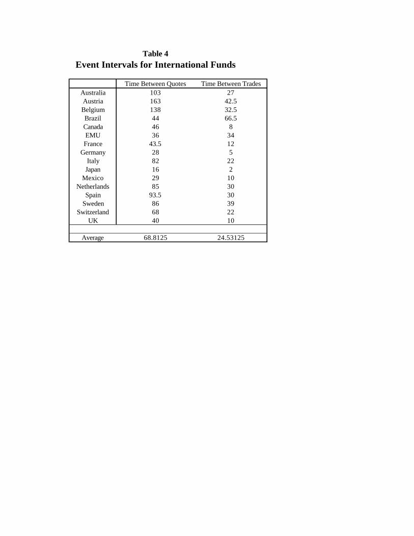
Table 4Event Intervals for International Funds

Time Between Quotes Time Between TradesAustralia 103 27Austria 163 42.5Belgium 138 32.5Brazil 44 66.5Canada 46 8EMU 36 34France 43.5 12

Germany 28 5Italy 82 22Japan 16 2

Mexico 29 10Netherlands 85 30

Spain 93.5 30Sweden 86 39

Switzerland 68 22UK 40 10

Average 68.8125 24.53125

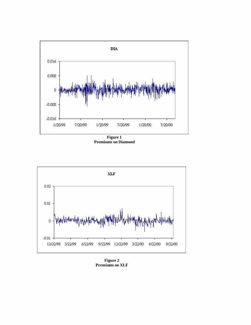
Figure 1

Premiums on Diamond

Figure 2 Premiums on XLF

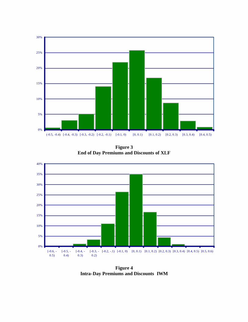
Figure 3

End of Day Premiums and Discounts of XLF

Figure 4

Intra-Day Premiums and Discounts IWM

0%

5%

10%

15%

20%

25%

30%

(-0.5, -0.4) [-0.4, -0.3) [-0.3, -0.2) [-0.2, -0.1) [-0.1, 0) [0, 0.1) [0.1, 0.2) [0.2, 0.3) [0.3, 0.4) [0.4, 0.5)

0%

5%

10%

15%

20%

25%

30%

35%

40%

[-0.6, -0.5)

[-0.5, -0.4)

[-0.4, -0.3)

[-0.3, -0.2)

[-0.2, -.1) [-0.1, 0) [0, 0.1) [0.1, 0.2) [0.2, 0.3) [0.3, 0.4) [0.4, 0.5) [0.5, 0.6)

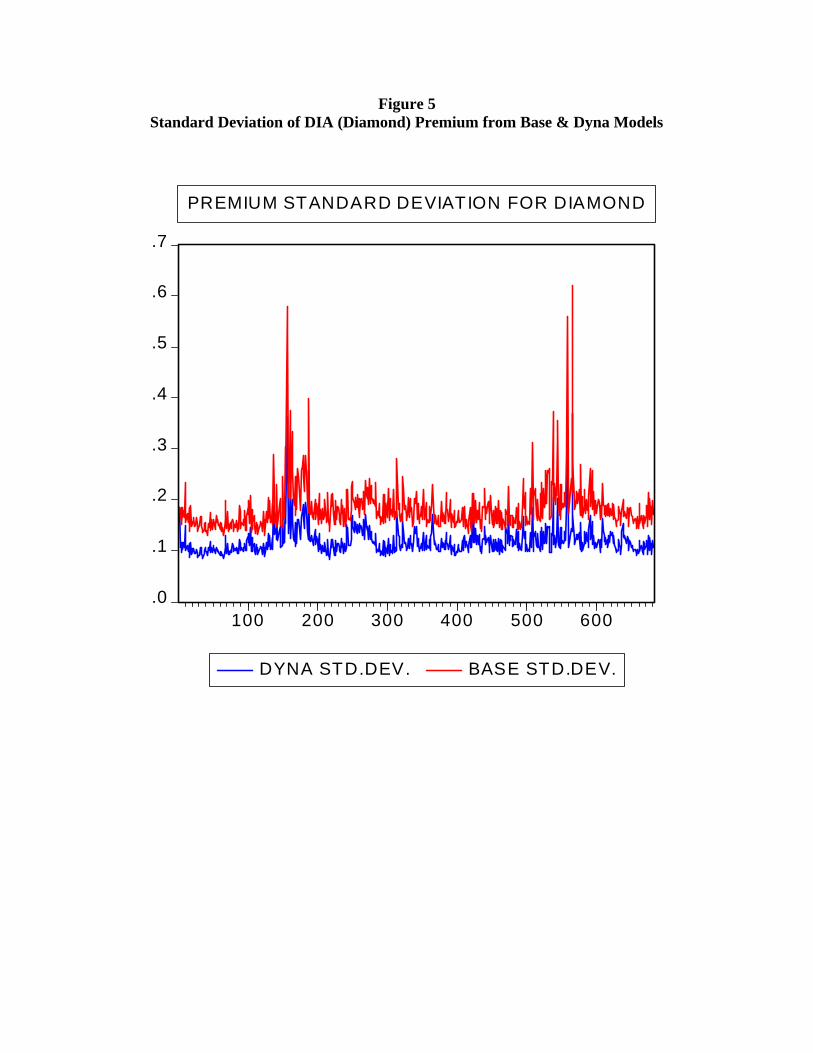
Figure 5 Standard Deviation of DIA (Diamond) Premium from Base & Dyna Models

.0

.1

.2

.3

.4

.5

.6

.7

100 200 300 400 500 600

DYNA STD.DEV. BASE STD.DEV.

PREMIUM STANDARD DEVIATION FOR DIAMOND

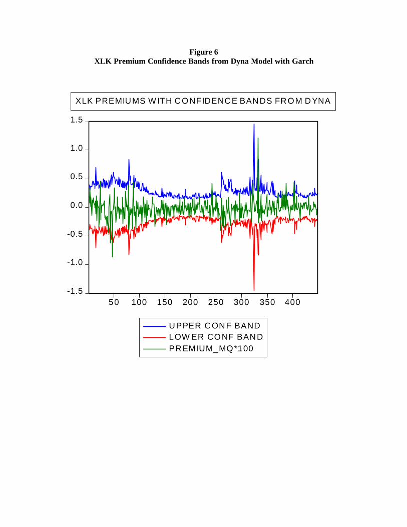
Figure 6 XLK Premium Confidence Bands from Dyna Model with Garch

-1.5

-1.0

-0.5

0.0

0.5

1.0

1.5

50 100 150 200 250 300 350 400

UPPER CONF BANDLOW ER CONF BANDPREMIUM_MQ*100

XLK PREMIUMS W ITH CONFIDENCE BANDS FROM DYNA

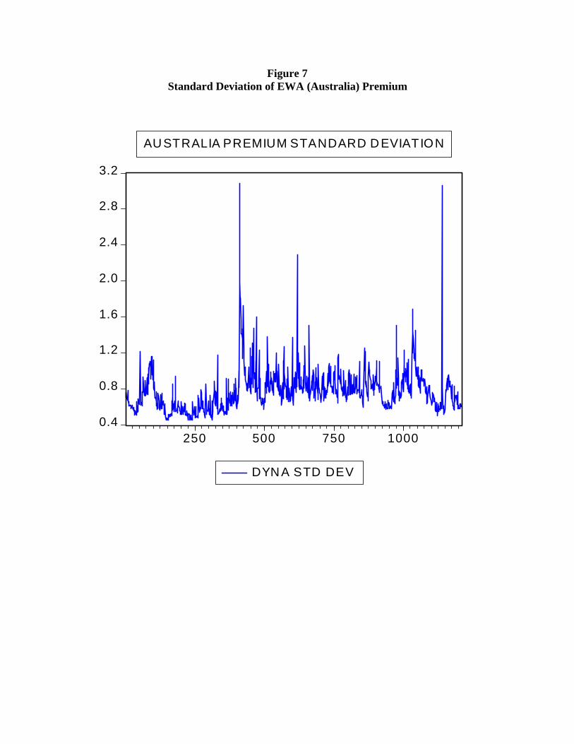
Figure 7 Standard Deviation of EWA (Australia) Premium

0.4

0.8

1.2

1.6

2.0

2.4

2.8

3.2

250 500 750 1000

DYN A STD DEV

AU STRALIA PREMIUM STANDARD D EVIATION

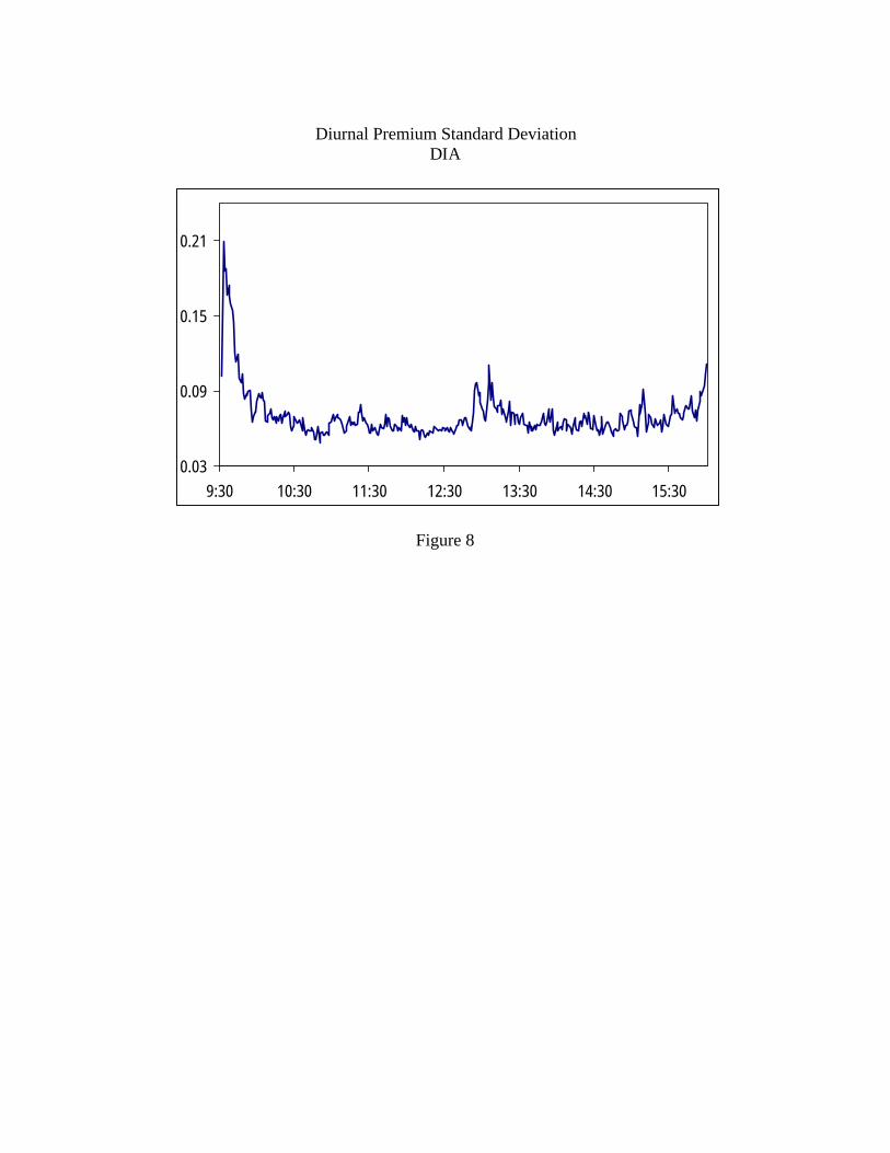
Diurnal Premium Standard Deviation

DIA

Figure 8

0.03

0.09

0.15

0.21

9:30 10:30 11:30 12:30 13:30 14:30 15:30