1

Pricing CDOs with State Dependent Stochastic Recovery Rates

Salah Amraoui, Laurent Cousot, Sébastien Hitier and Jean-Paul Laurent1

Revised: January, 2012

Abstract

Up to the 2007 crisis, research within bottom-up CDO models mainly concentrated on the dependence between defaults. Since then, due to substantial increases in market prices of systemic credit risk protection, more attention has been paid to recovery rate assumptions.

In this paper, we use stochastic orders theory to assess the impact of recovery on CDOs and show that, in a factor copula framework, a decrease of recovery rates leads to an increase of the expected loss on senior tranches, even though the expected loss on the portfolio is kept fixed. This result applies to a wide range of latent factor models and is not specific to the Gaussian copula model.

We then suggest introducing stochastic recovery rates in such a way that the conditional on the factor expected loss (or equivalently the large portfolio approximation) is the same as in the recovery markdown case. However, granular portfolios behave differently. We show that a markdown is associated with riskier portfolios that when using the stochastic recovery rate framework. As a consequence, the expected loss on a senior tranche is larger in the former case, whatever the attachment point.

We also deal with implementation and numerical issues related to the pricing of CDOs within the stochastic recovery rate framework. Due to differences across names regarding the conditional (on the factor) losses given default, the standard recursion approach becomes problematic. We suggest approximating the conditional on the factor loss distributions, through expansions around some base distribution.

Finally, we show that the independence and comonotonic cases provide some easy to compute bounds on expected losses of senior or equity tranches. Keywords: credit risk assessment, recovery rates, CDOs, stochastic orders. JEL subject classification. Primary G13, G32; Secondary C02, D46, D84, M41. MSC2000 subject classification. Primary 91B16, 91B28, 91B30, Secondary 60E15, 62H11. 1 Salah Amraoui (Structured Credit Derivatives Trader , BNP Paribas), Laurent Cousot (Quantitative Analyst, BNP Paribas), Sébastien Hitier (Quantitative Analyst, BNP Paribas), Jean-Paul Laurent (corresponding author, Professor, Université Paris 1 Panthéon-Sorbonne, PRISM & Labex Refi, 17, rue de la Sorbonne, 75005, Paris, France, laurent.jeanpaul@free.fr or jean-paul.laurent@univ-paris1.fr, http://laurent.jeanpaul.free.fr/ ). The authors thank the two referees, Xavier Burtschell, Laurent Carlier, Pierre Miralles, Thierry Rehmann for numerous and helpful comments. Additional feedbacks from Fakher Ben Atig, Areski Cousin, Michel Crouhy, Ersnt Eberlein, Jean-David Fermanian, Steven Hutt, Benjamin Jacquard, Marek Musiela, Olivier Vigneron and participants at the Large Portfolio Concentration and Granularity conference and at the third Financial Risks International Forum on Risk Dependencies have also been welcome. Jean-Paul Laurent acknowledges support from the BNP Paribas Cardif chair “Management de la Modélisation”. All errors are ours. The views expressed are the authors’ own and not necessarily those of BNP Paribas.

2

Introduction. The importance of recovery rate modelling in credit risk assessment has been recognized for a long time. Schuermann [2004], Altman et al. [2004], Altman et al. [2005], Altman [2006], Chava et al. [2008] provide a review of results and emphasize the negative correlation between default probabilities and recovery rates. Focusing on the tails on the loss distribution, Frye [2000a, 2000b], Pykhtin [2003], Chabaane et al. [2004, 2005] exhibit a dramatic increase of measures of credit risk and the need of extra economic capital to deal with the previous effect. In the credit derivatives field, as research on CDOs was considering alternatives to the Gaussian copula to account for tail risk, stochastic recovery rate effects started to be investigated. These were discussed in, among others, Andersen and Sidenius [2004], Gregory and Laurent [2004], Hull and White [2004]. It appeared that idiosyncratic recovery rate risk would rather well be diversified in senior tranches and that such recovery rate effects poorly explained the so-called correlation smiles2. Therefore, until the 2007 credit crisis, the standard method for quoting synthetic CDO tranches within investment banks was the one-factor Gaussian copula model with deterministic recovery consistent with flow CDS trading. Stochastic recovery models were not necessary to fit the market at that time and recovery distribution and correlation with losses was severely underspecified given the absence of market information concerning recovery in isolation. As the spreads of super-senior tranches increased during the credit crisis, market participants could not calibrate anymore correlation parameters from market data. A common interpretation of this breakdown is that if the number of defaulting assets increased to the point where the senior tranches are hit, the economy would be in a bad shape, one in which recovery rates would be expected to be low. Thus the relevant quantity for predicting a default payout is the recovery rate conditional on a tranche being hit, and not simply the individual names' expected recovery as used by vanilla credit default swap traders to convert a running spread to an upfront value and vice versa. Actually, Das and Hanouna [2008] show negative correlation between recovery rates and default probabilities in the risk-neutral world. This feature is included in the models studied by Amraoui and Hitier [2008], Krekel [2008], Bennani and Maetz [2009], Elouerkhaoui [2009], Kakodkar et al. [2009], Li [2009], Prampolini and Dinnis [2009]. This state dependent approach to recovery rates appears as a convenient way to fatten the right tail of portfolio loss distributions. It is further investigated in the paper and compared with the simpler approach of marking down the recovery rates, either on all names underlying the credit portfolio on or a subset of names. These analyses lead the path to a more accurate management of recovery rate risks within books of CDOs. 2 Let us notice that the notion of recovery rate in a CDO pricing context depends upon the precise definition of a default event and of the settlement procedures. This concerns especially the notion of restructuring and auction mechanism. Thus, one should use historical data with caution, as emphasized in Guo et al. [2008] or Verde et al. [2009]. Let us also stress that as far as CDO tranche pricing is involved, we need to consider the joint distribution of default times and recovery rates across all names, which also includes the cross-sectional dependence between recovery rates, which is not usually addressed in the econometrics literature. Eventually, one needs to consider risk-neutral recovery rates as in Pan and Singleton [2008].

3

The paper involves various concepts related to stochastic orders3 which appear to be the right tool to achieve our practical goal of comparing CDO models. Given this, we chose to proceed by gradual extensions. Various results and related proofs can be put in a larger setting. From time to time, we point this out, such as the use of other dependence structures than the Gaussian copula, or within the Gaussian copula framework, the use of multifactor models that can be useful in bespoke pricing. The paper is organized as follows:

- Section I studies the impact of recovery on the expected tranche losses in a deterministic recovery model. Section I also introduces the stochastic orders results that will be used throughout the paper.

- Section II recalls the stochastic recovery rate modelling framework introduced by Amraoui and Hitier [2008] and states some bounds and monotonicity results on recovery rates. It is shown that stochastic and deterministic recovery rates models share the same large portfolio approximations.

- Section III discusses the implementation and numerical issues related to the pricing of CDOs in the stochastic recovery framework. Subsection III.1 deals with large and granular portfolios. Subsection III.2 compares the conditional variances of portfolio losses in the stochastic recovery rate framework and under a recovery markdown. Pricing methods need to be updated in case of stochastic recovery rates. Thus, subsection III.3 is dedicated to the computation of CDO tranches using expansion techniques, while subsection III.4 investigates the accuracy of such approaches. Finally, subsection III.5 aims at comparing the pricing of tranches under a recovery markdown assumption and in the stochastic recovery framework.

- Section IV provides an account of the behaviour of CDO tranche premiums with respect to the correlation parameter. Subsection IV.1 deals with the comonotonic default dates case, while subsection IV.2 is dedicated to independent default dates. Subsection IV.3 deals with the behaviour of tranche premiums as the correlation parameter increases.

- Section V concludes.

Most mathematical proofs are postponed to the appendices. Default dependence modelling. As usual, we will be given some abstract probability space under which we can define a pricing measure . In the remainder of the paper, we consider a single time horizon t setting. As for the default indicators to time t , we consider the standard one factor Gaussian copula model: 1i iV V Vρ ρ= + − , where 0 1ρ≤ ≤ and

1, , , nV V V are independent standard Gaussian random variables. ( )1i i it V Pτ −≤ ⇔ ≤ Φ ,

where iτ is the default date of name i , ( )i iP F t= is the marginal probability that name i defaults before t 4 and Φ denotes the Gaussian distribution function. The default indicator

3 We refer to Müller and Stoyan [2002] or Shaked and Shanthikumar [2007] for textbooks that survey the topic. 4 For simplicity, we omit the dependence in t in the default probability iP .

4

associated with name i can then be written as: { } ( ){ }11 1i i i

t V Pτ −≤ ≤Φ= . ρ is known as the

tetrachoric correlation coefficient as opposed to the linear correlation of default indicators. The conditional default probabilities will be denoted by:

( ) ( ) ( )1

1i

i i

P Vt V P V

ρτ

ρ

− Φ −≤ = Φ = −

.

We chose to specify the dependence structure of default indicators instead of that of default times5. This choice of dependence structure is rather expository as will be stressed below, since most stated results hold for any latent factor model. I) Recovery impact on CDO tranches. In a first step, we consider how a deterministic recovery rate assumption drives the expected losses of senior tranches. The recovery rate for name i is denoted by iR and the corresponding loss given default iM . Note that the recovery rates do not need to be equal across names. One can predict the effect of a recovery markdown in a large number of dependence models associated with latent factors, including the above flat correlation Gaussian copula, on the expected loss of senior tranches. Actually, a recovery markdown leads to an increase of the expected loss of a senior tranche and a converse effect on an equity tranche6. This provides the sign of a recovery delta, when there is no premium leg, in almost all models used in the industry. Though the formal proofs depend upon the theory of stochastic orders, due to the non Gaussian features of risks involved, the way the loss variance moves gives us an intuition of the result. Let us discuss that now and consider a downward shift of a recovery rate

i i iR R R δ→ = − , 0iR δ≥ > . - The default probability decreases accordingly to iP so that the expected loss

associated with name i remains unchanged: ( ) ( )1 1i i i iR P R P− = − . In other words,

5 We refer the reader to Li [2009] for a discussion of the differences between the two approaches. Just as Gaussian correlation observed on equity tranches varies with maturity, which is compatible with the copula of default indicator approach, but not the copula of default time, the stochastic recovery model proposed here aims to be compatible with the copula of default indicators only. The CDO price can be obtained as a linear combination of options on the portfolio loss maturing at different times t . When practitioners are asked to price a linear combination of options, on different underlyings, the option model corresponding to each underlying is used rather than trying to come up with a model consistent with all the underlyings at once. 6 Part of this result is obvious. If the recovery rate goes down, say from 40% to 15%, then all senior tranches [ ],100%b with 60% 85%b≤ ≤ will have a zero premium with the 40% recovery assumption. With positive default probabilities, they obviously have a positive premium with the latter recovery rate assumption. The point that we make here is that this results remains true for all

[ ]0,1b∈ .

5

default frequency is smaller but the default magnitude is bigger. In the extreme case where 1iP = , the variance of the loss associated with name i is equal to zero. Simple algebra shows the larger iP , the smaller the variance of the loss associated with name i . So one can expect that the recovery markdown (thus a decrease of default probabilities) leads to an increase of the risk associated with name i .

- On the other hand, since all risks associated with different names are usually positively correlated, an increase in the variance of an individual risk leads to an increase in the variance of the portfolio loss. Therefore, one can expect an increase of the expected loss on senior tranches and conversely a decrease of the expected loss on equity tranches.

Let us now proceed to a rigorous analysis. As a first step, we need to compare the loss on name i before and after the markdown. Lemma I.1: Let us consider i iR R δ= − , with 0 1iR< < , 0iR δ≥ > and iP such that

( ) ( )1 1i i i iR P R P− = − , 1iP ≤ . Then:

( ) ( ){ } ( ) ( ){ }1 11 1 1 1i i i i

i cx iV P V PR R− −≤Φ ≤Φ

− ≤ − ,

where cx≤ stands for the convex order7. The proof of Lemma 1.1 is detailed in appendix A.1. Let us notice that this inequality between losses on name i before and after the markdown, with respect to the convex order, is not specific to the Gaussian copula. One should not be deceived about the use of Gaussian latent variables iV , which is here simply a matter of notational convenience. The (univariate) convex order involves a comparison between two marginal distributions. These are binary in both cases, taking values 0 with probability 1 iP− and 1 iR− with probability iP for the left hand term of the inequality and values 0 with probability 1 iP− and 1 iR− with probability iP for the right hand term8. This will be of importance when extending comparison results to a larger class of credit models.

7 We recall that given two random variables ,X Y , we say that X is smaller than Y with respect to the convex order, and we denote cxX Y≤ if [ ] [ ]( ) ( )E f X E f Y≤ for all convex functions f such that the expectations are well-defined. Convex order is a standard tool in actuarial studies and reliability theory. Since f Id= and f Id= − are convex, cxX Y≤ implies that [ ] [ ]E X E Y= . If we think of X and Y as losses, they can be compared with respect to the convex order only if they share the same expectation. Moreover, since 2x x→ is convex, we readily have:

[ ] [ ]cxX Y Var X Var Y≤ ⇒ ≤ . It can be shown that cxX Y≤ is equivalent to [ ] [ ]E X E Y= and

[ ] [ ]( ) ( )E u Y E u X≤ for all increasing and concave functions u . The latter condition means that X is less risky than Y with respect to second order stochastic dominance, commonly used in microeconomics. When ,X Y are Gaussian, that is equivalent to [ ] [ ]E X E Y= and ( ) ( )Var X Var Y≤ . 8 See appendix A for details about comparing the two distribution functions.

6

The next step is to compare the riskiness of portfolio losses that are sums of these individual losses. Since their distributions are not identical, the vectors of individual losses cannot be compared through the supermodular order, which was the key tool in Burtschell et al. [2008] or Cousin and Laurent [2008a]. One of the required mathematical tools is the comparison of random vectors through the directional convex order. Let us consider a function : nf → . We define the difference operator i

ε∆ , 0ε > , 1 i n≤ ≤ by ( )( ) ( )i if x f x e f xε ε∆ = + − , where ie is the i -th unit vector.

f is called directionally convex if for all 1 i j n≤ ≤ ≤ and , 0ε δ > , ( ) 0i j f xε δ∆ ∆ ≥ for all nx∈ 9.

Given two n - dimensional random vectors ,X Y , we say that X is smaller than Y with respect to the directionally convex order if ( ) ( )E f X E f Y≤ for all directionally

convex functions f such that the previous expectations are well-defined10. More details about the directional convex order can be found in Rüschendorf [2004]. We also need to consider a notion of positive dependence between the components of a random vector, which are here the individual losses. Definition: A random vector ( )1, , nX X X= is said to be conditionally increasing if

( ) ( )i j j JE X Xφ

∈

is increasing in the jX ’s for all { }1, ,J n⊂ , i J∉ and increasing

functions φ such that the expectation is well-defined. Let F be the joint distribution function of X and C a copula function associated with F . Proposition 3.5 of Müller and Scarsini [2001] states that if C is conditionally increasing11, then F is conditionally increasing. That makes clear that the notion of conditional increase is related to the dependence structure and not to the marginals. We may also note that if X is conditionally increasing the same applies to X− . We now recall a useful theorem from Müller and Scarsini [2001]. Theorem I.1: Let X and Y be random vectors with a common conditional increasing copula and assume that i cx iX Y≤ for all { }1, ,i n∈ . Then, dcxX Y≤ .

9 For any convex function :g → , ( ) ( )1 1, , n nf x x g x x= + + is directionally convex. For

instance, ( ) ( )1 1, , n nf x x x x K += + + − is directionally convex, which we will use for the analysis of senior tranches. 10 Let us notice that a directionally convex function is supermodular. As a consequence,

sm dcxX Y X Y≤ ⇒ ≤ , where sm≤ stands for the supermodular order. 11 Clearly the notion of conditional increase is law-invariant. Thus, we can compare distribution functions instead of the corresponding random vectors.

7

Let us now address the most usual case where dependence between default events is associated with a Gaussian copula. As a consequence, in the case of deterministic recovery rates, the individual losses also admit the same Gaussian copula. Usually too, the correlation matrix is associated with non negative terms. As discussed in Rüschendorf [1981], this notion of positive dependence is too weak, since it may not lead to conditional increase. However, it is simple to state whether a Gaussian vector is conditionally increasing (see Theorem 2 in Rüschendorf [1981] or Theorem 3.6 in Müller and Scarsini [2001]). Theorem I.2: Let us consider a Gaussian vector ( )1, , nV V with an invertible covariance matrix Σ . Then the following statements are equivalent:

a) ( )1, , nV V is conditionally increasing.

b) 1−Σ is a M -matrix. We recall that ( )

1 ,ij i j nA a

≤ ≤= is an M -matrix if 0ija ≤ , i j∀ ≠ , and if all principal minors are

positive. There are other characterizations of M -matrices. For instance, 1−Σ is an M -matrix if Σ is non singular, entrywise nonnegative and if 1−Σ has nonpositive off-diagonal entries. M -matrices have been used for a long time in connexion with Gaussian distributions (see Tong [1990]). Property I.1: Let us consider a Gaussian vector ( )1, , nV V associated with a “flat”

correlation structure 1i iV V Vρ ρ= + − , where 1, , , nV V V are independent standard Gaussian random variables and 0 1ρ< < . Then, the corresponding Gaussian copula is conditionally increasing. The proof of property 1.1 is detailed in appendix A.2. Note that this property can be extended to non flat correlation structures (see appendix A.3.1) and to some multifactor Gaussian vectors associated with intra-inter-class correlation matrices as defined by Eaton [1993] and used in a credit context by Gregory and Laurent [2004] (see appendix A.3.3). However we would like to emphasize the fact that not all factor models with positive factor loadings lead to conditional increasing copulas. We refer to appendix A.3.2 for more details. Property I.2: Given a Gaussian copula with flat correlation, 0 1ρ< < , the expected loss on a senior tranche increases after a recovery markdown while the converse applies to equity tranches. On mathematical grounds, this is a mere consequence of the stochastic inequality:

( ) ( ){ } ( ) ( ){ }1 1

1 11 1 1 1

i i i i

n n

i cx iV P V Pi i

R R− −≤Φ ≤Φ= =

− ≤ −∑ ∑ ,

where the left hand term corresponds to the portfolio loss before the markdown and the right hand term to the portfolio loss after the markdown. In other words, a markdown

8

actually leads to an increase of risk of the credit portfolio12. This property, whose proof is available in appendix A.3, is illustrated numerically in appendix A.4. Notice that no homogeneity assumption on default probabilities or recovery rates is required. In particular, we can think of applying a recovery markdown on a single name or a subset of names. Another remark concerns the losses conditional on the latent factor. These do change after the recovery markdown, thus the two models do not share the same large portfolio approximations. The previous analysis has been performed under the assumption of a Gaussian copula. For numerical illustrations, we refer to appendix A.5. To demonstrate the usefulness of the above techniques, we show in appendix A.6 how to deal with the case of Archimedean copulas, based on results of Müller and Scarsini [2001]. We obtain quite similar results since, in most useful cases, Archimedean copulas are conditionally increasing. We subsequently show that similar results also hold for most one factor models, including additive factor copulas, random factor loadings, frailty models, multivariate Poisson models, affine intensity models (see appendix A.7). The analysis is based on papers by Holland [1981], Holland and Rosenbaum [1986] about item response models and unidimensional monotone latent variable models. II) Stochastic Recovery Model. The use of recovery markdown is easy to handle but leads to substantial shifts in the valuation of a book of single name CDS: If the expected loss is unchanged, as assumed in section I, the value of the default legs of plain CDS remains the same. However, this does not hold for the value of premium legs, which involve only the default probabilities and not the recovery rates. The decrease of marginal default probabilities associated with a recovery markdown will increase the value of a long position in the premium leg of a CDS and therefore the value of a sell protection position on the CDS13. On the contrary, a suitable stochastic recovery rate modelling does not impact the expected losses on individual names nor the marginal default probabilities (and thus the value of a book of CDS) but typically puts more weight on large losses, which subsequently leads to a flatter base correlation structure. As we mentioned above, a flat base correlation structure is desirable since it usually eases the pricing of tranchelets14 and smooths out the credit spread deltas. 12 Stated slightly differently, while the expected loss is kept unchanged, all convex risk measures increase after a markdown. 13 A well-managed trading book of CDS is likely to behave as a portfolio of long positions in premiums legs of CDS, since it corresponds to the outcome of profitable CDS trades after hedging the default leg exposure. This is likely to change after the big bang CDS protocol since undoing a CDS trade will only result in an upfront premium. 14 Arbitrage opportunities such as negative tranchelet prices may occur if one uses spline interpolation without caution. These unpleasant effects occur less frequently when the base correlations associated with different detachment points are of the same magnitude.

9

We consider a suitable stochastic modelling of recovery rates, where those are related to the common factor driving default events. In such a framework, for a unit nominal, the loss given default on name i is related to the latent factor V and the marginal default probability iP by:

( ) ( )

( )

( )

1

min 1

11

1

i

ii

i

P V

M V RP V

ρ

ρ

ρρ

−

−

Φ − Φ − = − Φ −

Φ −

,

with min0 1iiR R≤ ≤ ≤ and ( ) ( )min1 1i

i i iP R P R− = − . This specification corresponds to the

stochastic recovery rate model introduced by Amraoui and Hitier [2008] and further discussed by Elouerkhaoui [2009], Kakodkar et al. [2009], Li [2009], Prampolini and Dinnis [2009]15. It can be shown that min

iR is a lower bound for the stochastic recovery rate. This bound can be name specific, though in the simplest case we can set min 0iR = , which guarantees that any senior tranche will be traded at a positive premium. As one could expect ( )iM V is decreasing in V . Thus, larger losses given default are related to more likely defaults. We refer to appendix B for more details and proofs of the stated results. The loss on name i can be written ( ) ( ){ }11

i ii V P

M V −≤Φ in the Gaussian copula case with

stochastic recovery rate. Since ( ) ( ){ } ( )1 min1 1i i

ii iV P

E M V P R−≤Φ

= − and given that

( ) ( )min1 1ii i iP R P R− = − , the expected loss associated with name i is the same in the

stochastic recovery and in the prior model with fixed recovery rate iR 16. While the exposition focuses on the Gaussian copula for ease of exposition, the stochastic recovery framework can readily be generalized to most factor models. As an example, let us consider a Clayton copula, belonging to the class of frailty models. The conditional default probabilities can be written as:

( ) ( )( )exp 1i it V V P θτ −≤ = − ,

15 Krekel [2008] is another example of a suitable stochastic recovery rate model for the pricing of CDO tranches. While our approach is associated with dichotomous individual losses, Krekel model can be viewed as a multivariate polytomous item response probit model, using the statistical terminology, which extends the standard multivariate dichotomous item response probit model associated with the Gaussian copula and fixed recovery. The use of factor models in that framework can be traced back to Bock and Lieberman [1970]. In the credit field, one may also notice that Krekel approach is quite similar to the one used by Gupton et al. [1997] in Creditmetrics. The only difference is that the former considers different levels of default severity while the latter concentrate on pre-default quality, by looking at rating migrations. 16 Since marginal default probabilities also remain unchanged, using the stochastic recovery rate model will have no effect on the value of a book of credit default swaps.

10

where V follows a standard Gamma distribution with shape parameter 1/θ , 0θ > and iP is the marginal default probability. The stochastic loss given default is then given by:

( ) ( ) ( )( )( )( )min

exp 11

exp 1ii

ii

V PM V R

V P

θ

θ

−

−

−= −

−,

with min0 1iiR R≤ ≤ ≤ and ( ) ( )min1 1i

i i iP R P R− = − , the latter equation having the same

economic meaning as in the Gaussian copula case. Then, the loss associated with name i in

the stochastic recovery rate model writes ( ) { }1i ii V PM V ≤ , with ln i

iUV

Vψ = −

, where ψ is

the Laplace transform associated with the above Gamma distribution and 1, , nU U are uniform random variables, 1, , ,nU U V being jointly independent (see Burtschell et al. [2008] for details). The corresponding individual loss associated with a markdown of the recovery rate to min

iR is provided by ( ) { }min1 1i i

iV PR≤

− .

We notice that losses given default are perfectly driven by the common factor, thus there is no idiosyncratic recovery rate risk there. The same feature is shared in the modelling of Nedeljkovic et al. [2009]. One can also notice that the correlation parameter ρ in the Gaussian copula case (θ in the Clayton copula case) impacts both the dependence between default indicators and the marginal distributions of recovery rates. This can be seen as a drawback of the approach, but also means the model is parsimonious, which we feel is quite important for effective risk management. III) Computation of CDO tranche premiums. III.1 Large portfolio approximations. The loss on the portfolio at time t , associated with the stochastic recovery rate model, is

given by: ( ) ( ){ }1

11

i i

n

i V Pi

L M V −≤Φ=

=∑ . We discuss in appendix C.1 some dynamic properties of

the portfolio loss and possible alternative models.

We denote by: ( ) ( )1

min1

11

nii

LPi

P VL E L V R

ρ

ρ

−

=

Φ − = = − Φ −

∑ . LPL is also known as the

large portfolio approximation and can be viewed as the limit of a series of portfolio losses where diversification of credit risk is achieved at the name level, idiosyncratic risks are wiped off and the portfolio is only driven by factor risk. Let us emphasize that the portfolio loss associated with the stochastic recovery rate model

( ) ( ){ }1

11

i i

n

i V Pi

L M V −≤Φ=

=∑ and the simpler markdown specification ( ) ( ){ }1min1

1 1i i

ni

V Pi

R −≤Φ=

−∑ share

the same large portfolio approximation. In mathematical terms, these two portfolios have the same conditional expected loss. This means that the stochastic recovery rate and the recovery markdown approaches will only differ for “granular” portfolios.

11

We show below that the expected loss on an equity tranche is smaller when considering the (granular) stochastic recovery rate model than in the corresponding large portfolio approximation. This is a straightforward extension of a well-known result in the case of deterministic recovery rates.

Property III.1: ( ) ( ) ( ) ( ){ }1

1

min1 1

1 11 i i

n nii

LP cx i V Pi i

P VL R L M V

ρ

ρ−

−

≤Φ= =

Φ − = − Φ ≤ = −

∑ ∑ , where cx≤

stands for the convex order. The proof is detailed in appendix C.2. The intuition is rather simple, since the large portfolio approximation wipes off idiosyncratic risks and is thus less risky than the corresponding granular portfolio. As a consequence of the convex order between LPL and L ,

( ) ( )LPE L K E L K+ + − ≤ − for all detachment points K . This provides a lower bound for

the default leg of senior tranches. Since [ ] [ ] ( )1

1n

LP i ii

E L E L R P=

= = −∑ , using call-put parity,

we also have the following inequalities regarding equity tranches: ( ) ( )min , min ,LPE L K E L K≤

17.

This provides a quite easy to compute upper bound for the default leg of equity tranches. III.2 Conditional variances of losses under stochastic recovery rate and markdown models. We recall that the portfolio losses associated with the stochastic recovery rate model and the simpler markdown specification have the same conditional expectation. It is interesting to go one step further and analyse the conditional variance of the portfolio losses in the two approaches: this gives some intuition about the differences in risk. Since the individual losses are conditionally independent upon the factor V in the two specifications, the conditional variance is the sum of conditional variances on individual losses. We will thereafter focus on the conditional variance of the individual loss associated with a given name (say i ).

Property III.2: ( ) ( ){ } ( ) ( ){ }1 1min1 1 1 ,i i i i

ii V P V P

Var M V V Var R V V− −≤Φ ≤Φ

≤ − ∀ ∈ .

See appendix C.3 for the proof. As a consequence, the conditional variance of the portfolio loss in the stochastic recovery rate model is smaller than the conditional variance of the portfolio loss with a deterministic recovery markdown18. Though this is not a formal proof, we may think that the prices of senior tranches in the stochastic recovery framework will be smaller than their counterparts

17 Actually, we do not need call-put parity since min( , )x x K→− is convex. 18 This obviously assumes that the markdown is done appropriately, i.e. expected losses are the same in the two models.

12

priced under a recovery markdown (the converse applying to equity tranches). This will be investigated rigorously in subsection III.5. Finally, higher cumulants of the conditional loss distribution, in the stochastic recovery rate model can be easily computed: the individual losses are (conditionally) independent and their (conditional) distribution is up to some scaling factor (the loss given default) a Bernoulli distribution. This will be helpful in further computations. III.3 Pricing of CDO tranches based on expansion techniques. In this subsection, we deal with numerical issues related to the pricing of CDO tranches in the proposed stochastic recovery framework. We describe a numerical procedure which leads to accurate and fast implementations. It is based on expansions of the conditional loss distributions around some base conditional distribution. These ideas are well-known in statistics and have already been exploited for financial applications such as option pricing or credit risk assessment19. In our framework, conditioning on the value of the systemic factor V (and then integrating over it) reduces the problem to the case where all losses given default are deterministic (equal to ( )iM V ) and the default indicators independent. In this context, the most commonly used algorithm is the one described by Andersen et al. [2003]. It works quite well

when all losses given default are equal, say 60%125

for a CDX or iTraxx tranche, which was

until 2007, the standard assumption. In the general case where losses given default differ from one name to another, one must first approximate the losses given default by multiples of a loss unit. This corresponds to our framework since the losses given default ( )iM V depend upon the marginal default probabilities and are thus name specific. The complexity of the recursion algorithm is inversely proportional to the size of the loss unit. To illustrate this phenomenon, let us examine the elementary case of a two names basket, whose losses given default are displayed in Table 1.

1M 2M Loss unit Case 1 60% 60% 60% Case 2 60% 59% 1%

Table 1: Highest loss units in two simple cases. We notice that a small change in the recovery assumption of the second name divides the optimal loss unit20 by a factor 60 and therefore multiplies the overall computation time by 19 This subsection does not aim at providing a full account of the relevant literature. It intends to show that existing expansion techniques can be well suited for the pricing of CDO tranches in our stochastic recovery framework. 20 Prampolini and Dinnis [2009] suggest some bucketing approach to deal with the curse of dimensionality. Assessing rigorously the discretization errors related to the choice of the loss unit is not a standard issue. For simplicity, we did not tolerate any approximation in the losses given default when computing the optimal loss unit in Table 1. Other numerical schemes do not rely on such

13

this same factor. This simple example makes clear why using this algorithm for the stochastic recovery model will result in computation times much longer than for its markdown counterpart for instance. The above issue can be dealt with approximations of the conditional on V loss distributions by perturbed distributions. These numerical methods originated from the simple assessment that the (conditional) loss distribution is known in the case of a homogeneous portfolio, with identical recovery rates, default probabilities and independent default times: it is simply a binomial distribution. Moreover, on one hand, this distribution can be well approximated by a normal distribution when the number of portfolio constituents increases, using the central limit theorem (see Varadhan [2001]). On the other hand, when n increases and the expected loss is kept constant, then a good approximation of the binomial distribution is the Poisson distribution, according to the law of rare events (see Taylor and Karlin [1984]). That is why it is not surprising that these approximations appeared in the literature as proxies for conditional loss distributions even in the case of non-homogeneous portfolios: for instance, Shelton [2004] used the Gaussian distribution to price CDO and CDO squared. El Karoui and Jiao [2007] and El Karoui et al. [2007] considered the Gaussian and the Poisson distributions as first order approximations to price CDOs, while O'Kane [2007] used the binomial distribution for the same purpose. However, the three distributions above match at most the first two (conditional) moments of the (conditional) loss distributions, whereas all of the conditional moments can be computed quite easily using the conditional independence assumption. One way to benefit from that and match higher conditional moments is actually to multiply the concerned distribution by a linear combination of associated orthogonal polynomials 21 . This corresponds to the well-known Type A Gram-Charlier series in the case of the Gaussian distribution. Once we have approximated the conditional distribution of the portfolio loss, an integration over the distribution of V is required to get for instance, the expected losses on CDO tranches. The latter integration is usually done using Gauss-Hermite quadrature for example. We now detail how this can be put into execution with respect to the Gaussian distribution. Expansions around the Poisson and the binomial distributions are detailed in appendices C.4 and C.5. In the case of the Gaussian distribution, the associated polynomials are the Hermite

polynomials. We will further consider L E L V

LL Vσ

− =

, the rescaled loss and we aim at

providing approximations of the conditional distribution of L . The conditional density function of the rescaled loss is approximated by:

approximation of the loss unit. The Fourier transform inversion method of Gregory and Laurent [2003] or the saddle point approximation scheme described in Martin et al. [2001] are among them. 21 Note that matching higher moments is sometimes achieved at the expense of the positivity of the measure in these constructions. Also, increasing the number of matched moments does not necessarily lead to more accurate approximations. We refer to Kolassa [2006] for an extensive discussion of such techniques.

14

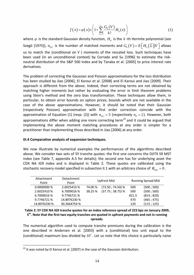
( ) ( ) ( )3

1 ( )!

GCnk

kk

G Vf x x H x

kϕ

=

= × +

∑ (1)

where ϕ is the standard Gaussian density function, kH is the k -th Hermite polynomial (see

Szegö [1975]), GCn is the number of matched moments and ( ) ( )k kG V E H L V = allows

us to match the (conditional on V ) moments of the rescaled loss. Such techniques have been used (in an unconditional context) by Corrado and Su [1996] to estimate the risk-neutral distribution of the S&P 500 index and by Tanaka et al. [2005] to price interest rate derivatives. The problem of correcting the Gaussian and Poisson approximations for the loss distribution has been studied by Jiao [2006], El Karoui et al. [2008] and El Karoui and Jiao [2009]. Their approach is different from the above. Indeed, their correcting terms are not obtained by matching higher moments but rather by evaluating the error in limit theorem problems using Stein's method and the zero bias transformation. These techniques allow them, in particular, to obtain error bounds on option prices, bounds which are not available in the case of the above approximations. However, it should be noted that their Gaussian (respectively Poisson) approximation with first order correction coincide with the approximation of Equation (1) (resp. (2)) with 3GCn = (respectively 2Pn = ). However, both approximations differ when adding one more correcting term22 and it could be argued that implementing the above moment matching procedures at any order is simpler for a practitioner than implementing those described in Jiao [2006] at any order. III.4 Comparative analysis of expansion techniques. We now illustrate by numerical examples the performances of the algorithms described above. We consider two sets of 5Y tranche quotes: the first one concerns the DJITX S9 MST index (see Table 7, appendix A.5 for details); the second one has for underlying asset the CDX NA IG9 index and is displayed in Table 2. These quotes are calibrated using the stochastic recovery model specified in subsection II.1 with an arbitrary choice of min 0R = .

Attachment Point

Detachment Point Upfront Mid Running Spread Mid

0.0000000 % 2.6025410 % 74.00 % (73.50 ; 74.50) % 500 (500 ; 500) 2.6025410 % 6.7009016 % 38.25 % (37.75 ; 38.75) % 500 (500 ; 500) 6.7009016 % 9.7746721 % 821.5 (814 ; 829) 9.7746721 % 14.8976230 % 470 (465 ; 475)

14.8976230 % 30.2664754 % 120 (115 ; 125)

Table 2: 5Y CDX NA IG9 tranche quotes for an index reference spread of 223 bps on January 2009, 5th. Note that the first two equity tranches are quoted in upfront payments and not in running

spreads.

The numerical algorithm used to compute tranche premiums during the calibration is the one described in Andersen et al. [2003] with a (conditional) loss unit equal to the (conditional) maximum loss divided by 710 . Let us note that this choice is particularly naive

22 It was noted by El Karoui et al. [2007] in the case of the Gaussian distribution.

15

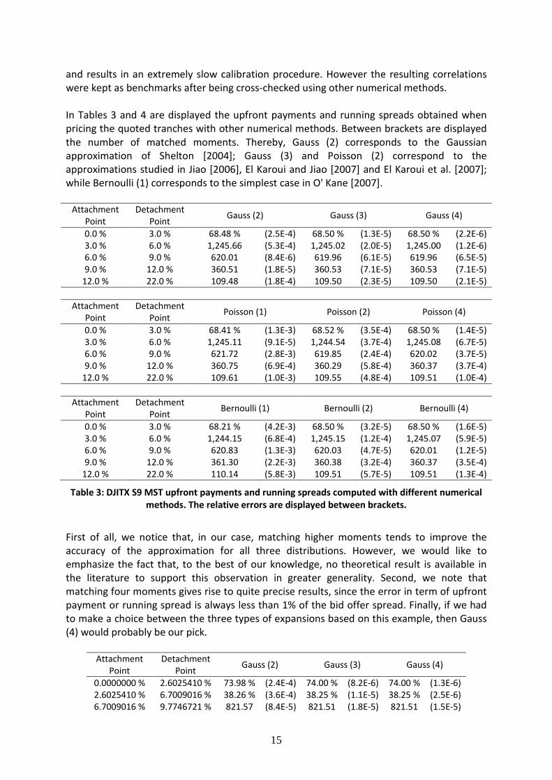
and results in an extremely slow calibration procedure. However the resulting correlations were kept as benchmarks after being cross-checked using other numerical methods. In Tables 3 and 4 are displayed the upfront payments and running spreads obtained when pricing the quoted tranches with other numerical methods. Between brackets are displayed the number of matched moments. Thereby, Gauss (2) corresponds to the Gaussian approximation of Shelton [2004]; Gauss (3) and Poisson (2) correspond to the approximations studied in Jiao [2006], El Karoui and Jiao [2007] and El Karoui et al. [2007]; while Bernoulli (1) corresponds to the simplest case in O' Kane [2007].

Attachment Point

Detachment Point Gauss (2) Gauss (3) Gauss (4)

0.0 % 3.0 % 68.48 % (2.5E-4) 68.50 % (1.3E-5) 68.50 % (2.2E-6) 3.0 % 6.0 % 1,245.66 (5.3E-4) 1,245.02 (2.0E-5) 1,245.00 (1.2E-6) 6.0 % 9.0 % 620.01 (8.4E-6) 619.96 (6.1E-5) 619.96 (6.5E-5) 9.0 % 12.0 % 360.51 (1.8E-5) 360.53 (7.1E-5) 360.53 (7.1E-5)

12.0 % 22.0 % 109.48 (1.8E-4) 109.50 (2.3E-5) 109.50 (2.1E-5)

Attachment Point

Detachment Point Poisson (1) Poisson (2) Poisson (4)

0.0 % 3.0 % 68.41 % (1.3E-3) 68.52 % (3.5E-4) 68.50 % (1.4E-5) 3.0 % 6.0 % 1,245.11 (9.1E-5) 1,244.54 (3.7E-4) 1,245.08 (6.7E-5) 6.0 % 9.0 % 621.72 (2.8E-3) 619.85 (2.4E-4) 620.02 (3.7E-5) 9.0 % 12.0 % 360.75 (6.9E-4) 360.29 (5.8E-4) 360.37 (3.7E-4)

12.0 % 22.0 % 109.61 (1.0E-3) 109.55 (4.8E-4) 109.51 (1.0E-4)

Attachment Point

Detachment Point Bernoulli (1) Bernoulli (2) Bernoulli (4)

0.0 % 3.0 % 68.21 % (4.2E-3) 68.50 % (3.2E-5) 68.50 % (1.6E-5) 3.0 % 6.0 % 1,244.15 (6.8E-4) 1,245.15 (1.2E-4) 1,245.07 (5.9E-5) 6.0 % 9.0 % 620.83 (1.3E-3) 620.03 (4.7E-5) 620.01 (1.2E-5) 9.0 % 12.0 % 361.30 (2.2E-3) 360.38 (3.2E-4) 360.37 (3.5E-4)

12.0 % 22.0 % 110.14 (5.8E-3) 109.51 (5.7E-5) 109.51 (1.3E-4)

Table 3: DJITX S9 MST upfront payments and running spreads computed with different numerical methods. The relative errors are displayed between brackets.

First of all, we notice that, in our case, matching higher moments tends to improve the accuracy of the approximation for all three distributions. However, we would like to emphasize the fact that, to the best of our knowledge, no theoretical result is available in the literature to support this observation in greater generality. Second, we note that matching four moments gives rise to quite precise results, since the error in term of upfront payment or running spread is always less than 1% of the bid offer spread. Finally, if we had to make a choice between the three types of expansions based on this example, then Gauss (4) would probably be our pick.

Attachment Point

Detachment Point Gauss (2) Gauss (3) Gauss (4)

0.0000000 % 2.6025410 % 73.98 % (2.4E-4) 74.00 % (8.2E-6) 74.00 % (1.3E-6) 2.6025410 % 6.7009016 % 38.26 % (3.6E-4) 38.25 % (1.1E-5) 38.25 % (2.5E-6) 6.7009016 % 9.7746721 % 821.57 (8.4E-5) 821.51 (1.8E-5) 821.51 (1.5E-5)

16

9.7746721 % 14.8976230 % 469.97 (6.5E-5) 469.99 (1.6E-5) 469.99 (1.5E-5) 14.8976230 % 30.2664754 % 119.98 (1.4E-4) 120.00 (9.2E-7) 120.00 (5.8E-8)

Attachment Point

Detachment Point Poisson (1) Poisson (2) Poisson (4)

0.0000000 % 2.6025410 % 73.91 % (1.2E-3) 74.03 % (4.1E-4) 74.00 % (3.4E-5) 2.6025410 % 6.7009016 % 38.24 % (1.8E-4) 38.24 % (2.8E-4) 38.25 % (9.2E-6) 6.7009016 % 9.7746721 % 822.82 (1.6E-3) 821.37 (1.6E-4) 821.69 (2.3E-4) 9.7746721 % 14.8976230 % 470.13 (2.8E-4) 469.85 (3.1E-4) 469.94 (1.2E-4)

14.8976230 % 30.2664754 % 120.08 (6.4E-4) 120.96 (3.1E-4) 120.00 (3.0E-5)

Attachment Point

Detachment Point Bernoulli (1) Bernoulli (2) Bernoulli (4)

0.0000000 % 2.6025410 % 73.64 % (4.9E-3) 73.99 % (8.4E-5) 74.00 % (1.5E-5) 2.6025410 % 6.7009016 % 38.15 % (2.6E-3) 38.25 % (5.9E-5) 38.25 % (4.7E-7) 6.7009016 % 9.7746721 % 822.83 (1.6E-3) 821.68 (2.2E-4) 821.64 (1.7E-4) 9.7746721 % 14.8976230 % 471.23 (2.6E-3) 469.93 (1.4E-4) 469.93 (1.4E-4)

14.8976230 % 30.2664754 % 120.70 (5.8E-3) 119.95 (4.0E-4) 119.98 (1.5E-4)

Table 4: CDX NA IG9 upfront payments and running spreads computed with different numerical methods. Between brackets are displayed the relative errors.

III.5 Recovery markdown and stochastic recovery model. We intend here to compare the computation of tranche spreads under the stochastic recovery model (with default probabilities iP ) and a granular Gaussian copula model with default probabilities iP , fixed recovery rates equal to min

iR . More precisely, we want to

compare ( ){ }1

1( )1

i i

n

i V Pi

M V −≤Φ=∑ and ( ) ( ){ }1min

11 1

i i

ni

V Pi

R −≤Φ=

−∑ . As stated above, these two portfolio

losses are associated with the same conditional expectation given V :

( ){ } ( ) ( ){ } ( ) ( )1 1

1

min min1 1 1

( )1 1 1 11i i i i

n n nii i

i V P V Pi i i

P VE M V V E R V R

ρ

ρ− −

−

≤Φ ≤Φ= = =

Φ − = − = − Φ − ∑ ∑ ∑ .

As before, we compare first the individual losses associated with the stochastic recovery model and with the recovery markdown. Let us first notice that the concept of convex order readily extends to conditional convex order. Given three random variables , ,X Y V , we will

say that VcxX Y≤ if ( ) ( )E f X V E f Y V ≤ for all convex functions f such that the

expectations are well-defined23. Clearly, due to the law of iterated expectations, we have: Vcx cxX Y X Y≤ ⇒ ≤ .

We can then claim that:

( ) ( ){ } ( ) ( ){ }1 1min1 1 1i i i i

V ii cxV P V P

M V R− −≤Φ ≤Φ≤ − .

The proof is quite simple and is detailed below.

23 Let us notice that V does not need to be scalar, though we do not need such an extension here.

17

From property II.1, ( ) min1 iiM V R≤ − . Thus, switching from ( )iM V to min1 iR− is simply a

conditional markdown. As for the default indicators, we can write them as ( )( ){ }11

i iV P V−≤Φ and

( )( ){ }11i iV P V−≤Φ

, where ( ) ( )1

1i

i

P VP V

ρρ

− Φ −= Φ −

and ( ) ( )1

1i

i

P VP V

ρ

ρ

− Φ − = Φ −

denote

the conditional default probabilities. Since i iP P≤ , ( ) ( )i iP V P V≤ . Going along the same lines as in the proof of Lemma I.1, we can state that the left-hand term of the above inequality is (conditionally on V ) less dangerous24 than the right hand term. Since the conditional expectations are both equal to ( )min1 ( )i

iR P V− , the conditional convex order

follows25. We now compare the risks associated with a recovery markdown and the above stochastic recovery rate model, as far as CDO tranches are concerned. Most of the tools used here can be found in Müller and Scarsini [2001] and the references therein. Given two n - dimensional random vectors ,X Y , we say that X is smaller than Y with respect to the componentwise convex order (and is denoted ccxX Y≤ ) if

( ) ( )E f X E f Y≤ for all componentwise convex functions26 f such that the previous

expectations are well-defined. As for the conditional convex order, this extends readily to the conditional on V case. The same generalisation also holds for the directionally convex order. Let us notice that V V

ccx dcxX Y X Y≤ ⇒ ≤ , using the same notational style as for the conditional convex order. Theorem 4.3 of Müller and Scarsini [2001] states that if ( )1, , nX X X= and ( )1, , nY Y Y= are random vectors with independent components and if i cx iX Y≤ for 1, ,i n= , then

ccxX Y≤ . This readily extends to the conditional on V case, which corresponds to our framework27. We can thus state:

( ){ } ( ){ } ( ) ( ){ } ( ) ( ){ }1 1 1 11 1 1 1

11 min min( )1 , , ( )1 1 1 , , 1 1

n n n n

V nn ccxV P V P V P V P

M V M V R R− − − −≤Φ ≤Φ ≤Φ ≤Φ

≤ − −

.

Thus, going into the same lines as in Property I.2, the portfolio losses can be compared through the conditional convex order and eventually through the convex order:

24 See the proof of Lemma 1.1 where the notion of “less dangerous” is detailed. 25 The conditional convex order implies that:

( ) ( ){ } ( ) ( ){ }1 1min1 1 1 ,i i i i

ii V P V P

Var M V V Var R V V− −≤Φ ≤Φ ≤ − ∀ ∈

,

which was already stated and proven in subsection III.2 through a direct computation. 26 A real-valued function f defined on n

is said to be componentwise convex if it is convex in each argument when the other are held fixed. 27 Conditionally on V , the individual losses

( ){ }1( )1i i

i V PM V −≤Φ

, 1, ,i n= are independent. The same

conditional independence result holds for the set of individual losses ( ) ( ){ }1min1 1i i

iV P

R −≤Φ− , 1, ,i n= .

18

( ){ } ( ) ( ){ }1 1min1 1

( )1 1 1i i i i

n ni

i cxV P V Pi i

M V R− −≤Φ ≤Φ= =

≤ −∑ ∑ .

As a consequence the expected losses on senior tranches are larger when applying a recovery markdown than when using the stochastic recovery rate model; the converse applies to equity tranches28. Let us now proceed through a numerical study to assess the discrepancies between the recovery markdown and the stochastic recovery model. The numerical tests that we performed validate the idea that a recovery markdown is associated with smaller expected losses on equity tranches than in the case of a granular stochastic recovery rate model. In the case studied in section I, we computed expected tranche losses at a given maturity in both the stochastic recovery model (with min 0%iR = ) and its markdown counterpart for different correlation assumptions. The results, displayed in Table 5, are hopefully in accordance with the theoretical analysis.

Correlation Model [0 , 3] % [0 , 6] % [0 , 9] % [0 , 12] % [0 , 22] % [0,100]%

10% M.D. 2.513% 3.880% 4.471% 4.703% 4.833% 4.838% S.R. 2.597% 3.965% 4.519% 4.725% 4.835% 4.838%

30% M.D. 1.983% 3.061% 3.697% 4.091% 4.642% 4.838% S.R. 2.041% 3.110% 3.733% 4.116% 4.651% 4.838%

50% M.D. 1.563% 2.439% 3.023% 3.440% 4.215% 4.838% S.R. 1.606% 2.474% 3.050% 3.461% 4.226% 4.838%

70% M.D. 1.204% 1.907% 2.414% 2.806% 3.655% 4.838% S.R. 1.235% 1.932% 2.434% 2.822% 3.666% 4.838%

90% M.D 0.891% 1.438% 1.853% 2.190% 3.001% 4.838% S.R. 0.910% 1.453% 1.866% 2.202% 3.005% 4.838%

Table 5: DJITX S9 MST expected tranche losses expiring on 06/20/11 for different correlation scenarios in the stochastic recovery model (S.R.) and in its markdown counterpart (M.D.).

We recall that in the 100% correlation case, the two models lead to the same expected tranche losses. Let us also notice that the discrepancies between the two approaches are small. This is not surprising since the large portfolio approximations are the same in the two cases and the granularity of the DJITX is not too large. IV) Dependence of CDO tranche premiums with respect to correlation.

28 Let us notice that the previous proof only applies when expected conditional losses are equal, which was not the case for instance in the recovery markdown case studied in section I. However, we stress that the above comparison result between a markdown and the corresponding stochastic recovery rate model is not specific to the Gaussian copula case. To follow up the Clayton copula case and using the same notations as above, we have ( ) { } ( ) { }min1 1 1

i i i i

V ii cxV P V PM V R≤ ≤≤ − since

( ) min1 iiM V R≤ − . Due to conditional independence upon V , we also have:

{ } { }( ) ( ) { } ( ) { }( )1 1 1 1

11 min min( )1 , , ( )1 1 1 , , 1 1

n n n n

V nn ccxV P V P V P V PM V M V R R≤ ≤ ≤ ≤

≤ − − .

Thus, portfolio losses when applying a recovery markdown and when using the stochastic recovery rate model are ordered the same way as in the Gaussian copula case.

19

The analysis is more complicated here since, as mentioned above, the correlation parameter is involved both in default dependence and in the distribution of losses given default. IV.1 Study of comonotonic default dates. When 100%ρ = , default dates 1, , nτ τ are comonotonic. This assumption leads to a lower bound for the expected loss on equity tranches. We recall that the loss given default on name i is provided by:

( ) ( )

( )

( )

1

min 1

11

1

i

ii

i

P V

M V RP V

ρ

ρ

ρρ

−

−

Φ − Φ − = − Φ −

Φ −

which depends upon the correlation parameter ρ 29.

Property IV.1: the portfolio loss associated with a correlation parameter 100%ρ = is

provided by: ( ) ( ){ }1min1

1 1i

ni

V Pi

R −≤Φ=

−∑ .

The proof of the previous property is detailed in appendix D.1. In other words, the limit case

100%ρ = collapses to a one factor Gaussian copula case, with perfect correlation, a deterministic recovery markdown to min

iR and marginal default probabilities equal to iP . Property IV.2: The 100% correlation case provides an upper bound for the expected loss on senior tranches and a lower bound for the expected loss on equity tranches. The proof of previous property is postponed in appendix D.2. The perfect correlation case provides an easy to compute upper bound for the default leg of senior tranches and a lower bound for the expected loss on equity tranches. IV.2 Study of independent default dates. When 0%ρ = , default dates 1, , nτ τ are independent. Since ρ also drives the recovery

rate, we readily have that ( ) 1i iM V R= − . In this limit case, the stochastic recovery rate becomes non stochastic and is equal to iR . The conditional default probabilities do not depend anymore upon V and are equal to iP . As a consequence, the stochastic recovery rate model is formally equivalent to a flat Gaussian copula model, with correlation parameter equal to zero, marginal default probabilities and constant recovery rates respectively equal to iP and , 1, ,iR i n= . The portfolio loss associated with 0%ρ = (independent default dates) is simply provided by:

( ) ( ){ }1

11 1

i i

n

i V Pi

R −≤Φ=

−∑ .

29 For notational simplicity the dependence of the loss given default upon ρ is not stated explicitly.

20

One can guess that 0ρ > leads to smaller values of the default leg of an equity tranche than in the case of independent default dates. We will show this in several steps. Technicalities are postponed to appendix D. First, we compare the loss associated with name i in the case of a constant recovery rate iR and default probability iP and in the case of a stochastic recovery rate with minimum recovery rate min

iR and corresponding parameter iP . Lemma IV.1: The loss associated with name { }1, ,i n∈ is smaller, with respect to the convex order, in the independence case than in the model with positive correlation:

( ) ( ){ } ( ) ( ){ }1 11 1 1i i i i

i cx iV P V PR M V− −≤Φ ≤Φ

− ≤ .

We then need to study the dependence structure between the individual losses. This is addressed in the following lemma.

Lemma IV.2: ( ) ( ){ } ( ) ( ){ }1 11 1

1 1 , , 1n n

nV P V PM V M V− −≤Φ ≤Φ

is weakly associated in sequence.

We recall that a random vector ( )1, , nX X is weakly associated in sequence if for all x∈ ,

1 1i n≤ ≤ − and non-decreasing function f , we have: { } ( )( )( 1)1 , 0i iX xCov f X +> ≥ , where

( )( 1) 1, ,i i nX X X+ += . This notion of positive dependence will be useful to show our main result.

Property IV.3: ( ) ( ){ } ( ) ( ){ }1 1

1 11 1 1

i i i i

n n

i cx iV P V Pi i

R M V− −≤Φ ≤Φ= =

− ≤∑ ∑ .

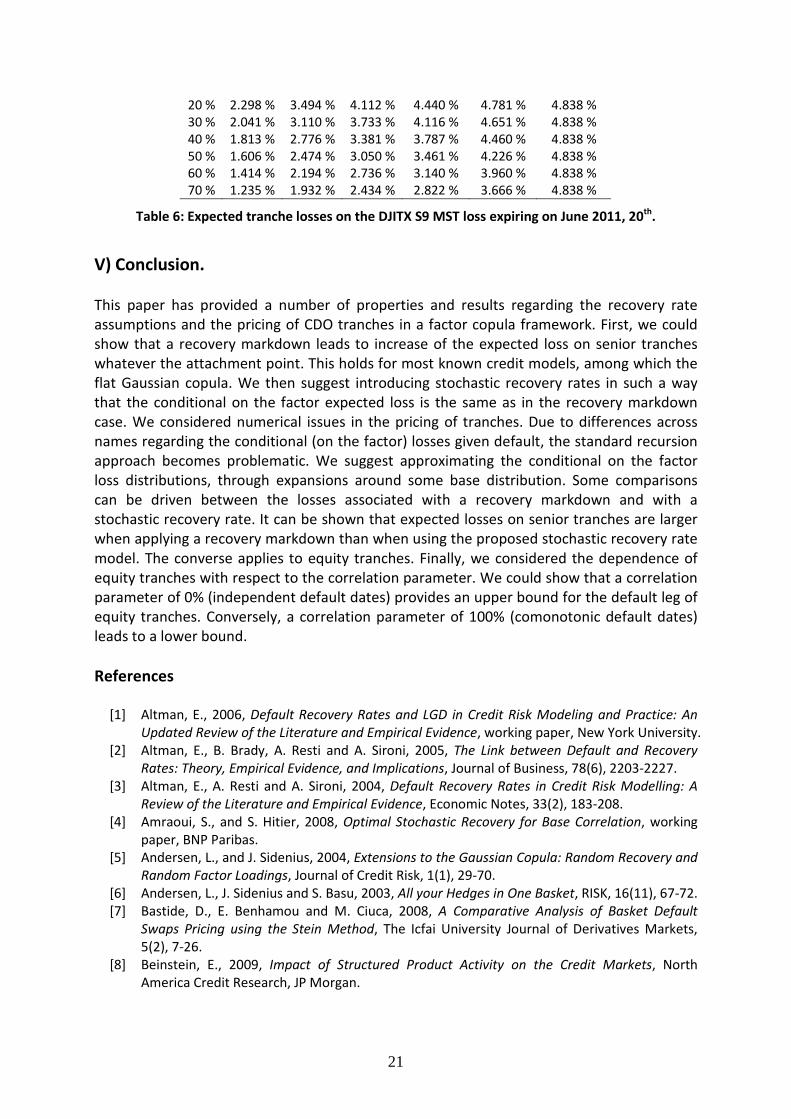
We recall that the right-hand term of the inequality corresponds to the portfolio loss in the independence case, while the left-hand term is the portfolio loss in the stochastic recovery model for a correlation parameter ρ . Thus, Property IV.3 is a formal statement that 0ρ > leads to smaller values of the default leg of an equity tranche than in the case of independent default dates. IV.3 Empirical study of monotonicity with respect to ρ . We have already shown that 0%ρ = and 100%ρ = are associated with bounds on the expected loss of base or senior tranches. We also know that, for large portfolios, the stochastic recovery model behaves as a standard Gaussian copula with a recovery markdown. In the latter case, we can state some monotonicity properties with respect to the correlation parameter. We may think of a similar behaviour in the case of the stochastic recovery model. To support our intuition, we considered the numerical example of section I and computed, for different correlation assumptions, expected tranche losses expiring on June 2011, 20th. The results, shown in Table 6, confirm what we expected: these quantities are decreasing with correlation.

Rho [0 , 3] % [0 , 6] % [0 , 9] % [0 , 12] % [0 , 22] % [0 , 100] %

21

20 % 2.298 % 3.494 % 4.112 % 4.440 % 4.781 % 4.838 % 30 % 2.041 % 3.110 % 3.733 % 4.116 % 4.651 % 4.838 % 40 % 1.813 % 2.776 % 3.381 % 3.787 % 4.460 % 4.838 % 50 % 1.606 % 2.474 % 3.050 % 3.461 % 4.226 % 4.838 % 60 % 1.414 % 2.194 % 2.736 % 3.140 % 3.960 % 4.838 % 70 % 1.235 % 1.932 % 2.434 % 2.822 % 3.666 % 4.838 %

Table 6: Expected tranche losses on the DJITX S9 MST loss expiring on June 2011, 20th.

V) Conclusion. This paper has provided a number of properties and results regarding the recovery rate assumptions and the pricing of CDO tranches in a factor copula framework. First, we could show that a recovery markdown leads to increase of the expected loss on senior tranches whatever the attachment point. This holds for most known credit models, among which the flat Gaussian copula. We then suggest introducing stochastic recovery rates in such a way that the conditional on the factor expected loss is the same as in the recovery markdown case. We considered numerical issues in the pricing of tranches. Due to differences across names regarding the conditional (on the factor) losses given default, the standard recursion approach becomes problematic. We suggest approximating the conditional on the factor loss distributions, through expansions around some base distribution. Some comparisons can be driven between the losses associated with a recovery markdown and with a stochastic recovery rate. It can be shown that expected losses on senior tranches are larger when applying a recovery markdown than when using the proposed stochastic recovery rate model. The converse applies to equity tranches. Finally, we considered the dependence of equity tranches with respect to the correlation parameter. We could show that a correlation parameter of 0% (independent default dates) provides an upper bound for the default leg of equity tranches. Conversely, a correlation parameter of 100% (comonotonic default dates) leads to a lower bound. References

[1] Altman, E., 2006, Default Recovery Rates and LGD in Credit Risk Modeling and Practice: An Updated Review of the Literature and Empirical Evidence, working paper, New York University.

[2] Altman, E., B. Brady, A. Resti and A. Sironi, 2005, The Link between Default and Recovery Rates: Theory, Empirical Evidence, and Implications, Journal of Business, 78(6), 2203-2227.

[3] Altman, E., A. Resti and A. Sironi, 2004, Default Recovery Rates in Credit Risk Modelling: A Review of the Literature and Empirical Evidence, Economic Notes, 33(2), 183-208.

[4] Amraoui, S., and S. Hitier, 2008, Optimal Stochastic Recovery for Base Correlation, working paper, BNP Paribas.

[5] Andersen, L., and J. Sidenius, 2004, Extensions to the Gaussian Copula: Random Recovery and Random Factor Loadings, Journal of Credit Risk, 1(1), 29-70.

[6] Andersen, L., J. Sidenius and S. Basu, 2003, All your Hedges in One Basket, RISK, 16(11), 67-72. [7] Bastide, D., E. Benhamou and M. Ciuca, 2008, A Comparative Analysis of Basket Default

Swaps Pricing using the Stein Method, The Icfai University Journal of Derivatives Markets, 5(2), 7-26.

[8] Beinstein, E., 2009, Impact of Structured Product Activity on the Credit Markets, North America Credit Research, JP Morgan.

22

[9] Bennani, N., and J. Maetz, 2009, A Spot Recovery Rate Extension of the Gaussian Copula, Barclays Capital, working paper.

[10] Bock, R. D., and M. Lieberman, 1970, Fitting a Response Model for n Dichotomously Scored Items, Psychometrika, 35(2), 179-197.

[11] Burtschell, X., J. Gregory and J-P. Laurent, 2007, Beyond the Gaussian Copula: Stochastic and Local Correlation, Journal of Credit Risk, 3(1), 31-62.

[12] Burtschell, X., J. Gregory and J-P. Laurent, 2008, A Comparative Analysis of CDO Pricing Models, in The Definitive Guide to CDOs: Market, Valuation, Application and Hedging, Chapter 15, 389-427, (G. Meissner ed.), Risk Books.

[13] Chabaane, A., J-P. Laurent and J. Salomon, 2005, Credit Risk Assessment and Stochastic LGD’s: An Investigation of correlation effects, in Recovery Risk: The Next Challenge in Credit Risk Management, E. Altman, A. Resti, A. Sironi (eds), Risk Publications (London).

[14] Chabaane, A., J-P. Laurent and J. Salomon, 2004, Double Impact: Credit Risk Assessment and Collateral Value, Revue Finance, 25, 157-178.

[15] Chava, S., C. Stefanescu and S. Turnbull, 2008, Modeling the Loss Distribution, working paper, University of Houston.

[16] Christofides T. C., and E. Vaggelatou, 2004, A Connection between Supermodular Ordering and Positive/Negative Association, Journal of Multivariate Analysis, 88(1), 138-151.

[17] Colangelo, A., M. Scarsini and M. Shaked, 2005, Some Notions of Multivariate Positive Dependence, Insurance: Mathematics and Economics, 37(1), 13-26.

[18] Corrado, C., and T. Su, 1996, Skewness and Kurtosis in S&P 500 Index Returns Implied by Option Prices, Journal of Financial Research, 19 (2), 175-192.

[19] Cousin, A., and J-P. Laurent, 2008a, Comparison Results for Exchangeable Credit Risk Portfolios, Insurance: Mathematics and Economics, 42(3), 1118-1127.

[20] Cousin, A., and J-P. Laurent, 2008b, An Overview of Factor Modeling for CDO Pricing, in Frontiers in Quantitative Finance: Credit Risk and Volatility Modeling, Chapter 7, 185-216, R. Cont (ed.), Wiley.

[21] Das S. R., and P. Hanouna, 2008, Implied Recovery, working paper, Santa Clara University. [22] Dhaene, J., M. Denuit, M. J. Goovaerts, R. Kass and D. Vyncke, 2002, The Concept of

Comonotonicity in Actuarial Science and Finance: Theory, Insurance: Mathematics and Economics, 31(1), 3-33.

[23] Dhaene, J., and M. J. Goovaerts, 2005, Dependency of Risks and Stop-Loss Order, ASTIN Bulletin, 26(2), 201-212.

[24] Eaton, M. L., 1993, A Group Action on Covariances with Applications to the Comparison of Linear Normal Experiments, in: M. Shaked, Y. L. Tong (Eds.), Stochastic Inequalities, IMS Lecture Notes Monograph Series, Vol. 22, Institute of Mathematical Statistics, Hayward, CA, 76-90.

[25] Eckner, A., 2007, Computational Techniques for Basic Affine Models of Portfolio Credit Risk, working paper, Stanford University.

[26] El Karoui, N., and Y. Jiao, 2009, Stein's Method and Zero Bias Transformation for CDO Tranche Pricing, Finance and Stochastics, 13(2), 151-180.

[27] El Karoui, N., Y. Jiao and D. Kurtz, 2008, Gauss and Poisson Approximation: Applications to CDOs Tranche Pricing, working paper, École Polytechnique.

[28] Elouerkhaoui, Y., 2009, Base Correlation Calibration with a Stochastic Recovery Model, working paper, Citigroup Global Markets.

[29] Embrechts, P., A. J. McNeil and D. Straumann, 2002, Correlation and Dependence in Risk Management: Properties and Pitfalls, In: Risk Management: Value at Risk and Beyond (M. Dempster, Ed.), Cambridge University Press, Cambridge, 176-223.

[30] Frye, J., 2000a, Collateral Damage, RISK, 13(4), 91-94. [31] Frye, J., 2000b, Depressing Recoveries, RISK, 13(11), 108-11. [32] Gregory, J., and J-P. Laurent, 2003, I Will Survive, RISK, 16(6), 103-107.

23

[33] Gregory, J., and J-P. Laurent, 2004, In the Core of Correlation, RISK, 17(10), 87-91. [34] Guo, X, R. A. Jarrow and H. Lin, 2008, Distressed Debt Prices and Recovery Rate Estimation,

Review of Derivatives Research, 11(3), 171-204. [35] Gupton, G. M, C. C. Finger and M. Bhatia, 1997, CreditMetrics - Technical Document, J.P.

Morgan. [36] Herbertsson, A., 2008, Pricing Synthetic CDO Tranches in a Model with Default Contagion: the

Matrix Analytic Approach, Journal of Credit Risk, 4(4), 3-35. [37] Hoeffding, W., 1940, Masstabinvariante Korrelationstheorie, Schriften des Mathematischen

Instituts und des Instituts für Angewandte Mathematik der Universität Berlin, 5, 179-233. [38] Holland, P. W., 1981, When are Item Response Models Consistent with Observed Data?,

Psychometrica, 46(1), 79-92. [39] Holland, P. W., and P. R. Rosenbaum, 1986, Conditional Association and Unidimensionality in

Monotone Latent Variable Models, The Annals of Statistics, 14(4), 1523-1543. [40] Hull, J., and A. White, 2004, Valuation of a CDO and an nth to Default CDS without Monte

Carlo Simulation, Journal of Derivatives, 2, 8-23. [41] Jiao, Y., 2006, Risque de Crédit : Modélisation et Simulation Numérique, Thèse de Doctorat,

École Polytechnique. [42] Joag-dev, K, M., D. Perlman and L. D. Pitt, 1983, Association of Normal Random Variables and

Slepian’s Inequality, Annals of Probability, 11(2), 451-455. [43] Kakodkar, A., S. Bandreddi, S. Tanna, R. Shi and R. Ramachandran, 2009, Coping with the

Copula, Merrill Lynch, Credit Derivatives Strategy, working paper. [44] Karlin, S., 1968, Total Positivity, Stanford University Press, Stanford, Calif. [45] Karlin, S., and Y. Rinott, 1980, Classes of Orderings of Measures and Related Correlation

Inequalities. I. Multivariate Totally Positive Distributions, Journal of Multivariate Analysis, 10(4), 467-498.

[46] Kimberling, C. H., 1974, A Probabilistic Interpretation of Complete Monotonicity, Aequationes Mathematicae, 10(2-3), 152-164.

[47] Kolassa, J. E., 2006, Series Approximation Methods in Statistics, Third Edition, Lecture Notes in Statistics 88, Springer Verlag, New York.

[48] Krekel, M., 2008, Pricing distressed CDOs with Base Correlation and Stochastic Recovery, working paper, UniCredit Markets & Investment Banking.

[49] Kurata, H, 2004, Inequalities Associated with Intra-Inter-Class Correlation Matrices, Journal of Multivariate Analysis, 88(2), 207-221.

[50] Laurent, J-P., and J. Gregory, 2005, Basket Default Swaps, CDOs and Factor Copulas, Journal of Risk, 7(4), 103-122.

[51] Li, Y., 2009, A Dynamic Correlation Modelling Framework with Consistent Stochastic Recovery, working paper, Quantitative Analytics, Barclays Capital.

[52] Marshall, A. W., and I. Olkin, 1988, Families of Multivariate Distributions, Journal of the American Statistical Association, 83(403), 834-841.

[53] Martin, R., K. Thompson and C. Browne, 2001, Talking to the Saddle, RISK, 14(6), 91-94. [54] McNeil, A. J., and J. Neslehova, 2008, Multivariate Archimedean Copulas, d -monotone

Functions and 1 - norm Symmetric Distributions, working paper, Maxwell Institute for the Mathematical Sciences.

[55] Müller, A., 2001, Stochastic Ordering of Multivariate Normal Distributions, Annals of the Institute of Statistical Mathematics, Vol. 53, N° 3, 567-575.

[56] Müller, A., and M. Scarsini, 2000, Some Remarks on the Supermodular Order, Journal of Multivariate Analysis, 73, 107-119.

[57] Müller, A., and M. Scarsini, 2001, Stochastic Comparison of Random Vectors with a Common Copula, Mathematics of Operations Research, Vo. 26., No. 4, 723-740.

[58] Müller, A., and M. Scarsini, 2005, Archimedean Copulae and Positive Dependence, Journal of Multivariate Analysis, 93(2), 434-445.

24

[59] Müller, A., and D. Stoyan, Comparison Methods for Stochastic Models and Risks, Wiley, 2002. [60] Nedeljkovic, J., D. Rosen and D. Saunders, 2009, Pricing and Hedging CLOs with Implied Factor

Models, working paper, The Fields Institute for Research in Mathematical Sciences. [61] O'Kane, D., 2007, Approximating Independent Loss Distributions with an Adjusted Binomial

Distribution, working paper, EDHEC Business School. [62] Pan, J., and K. J. Singleton, 2008, Default and Recovery Implicit in the Term Structure of

Sovereign CDS Spreads, Journal of Finance, 63(5), 2345-2384. [63] Pitt, L. D., 1983, Positively Correlated Normal Variables are Associated, Annals of Probability,

10(2), 496-499. [64] Prampolini, A., and M. Dinnis, 2009, CDO Mapping with Stochastic Recovery, working paper,

HSH Nordbank, available on www.defaultrisk.com. [65] Pykhtin, M., 2003, Unexpected Recovery Risk, RISK, 16(8), 74-78. [66] Rüschendorf, L., 2004, Comparison of Multivariate Risks and Positive Dependence, Journal of

Applied Probability, 41(2), 391-406. [67] Schönbucher, P., and D. Schubert, 2001, Copula-Dependent Default Risk in Intensity Models,

working paper, Bonn University. [68] Schuermann, T., 2004, What Do We Know About Loss Given Default?, working paper, Federal

Reserve Bank of New York. [69] Shaked, M., and J. G. Shanthikumar, 2007, Stochastic Orders, Springer. [70] Shelton, D., 2004, Back to Normal, Proxy Integration: A Fast Accurate Method for CDO and

CDO-squared Pricing, technical report, Citigroup Structured Credit Research. [71] Szegö, G., 1975, Orthogonal Polynomials, American Mathematical Society, Colloquium

Publications, Volume 23. [72] Tanaka, K., T. Yamada and T. Watanabe, 2005, Approximation of Interest Rate Derivatives'

Prices by Gram-Charlier Expansion and Bond Moments, working paper, IMES, Bank of Japan. [73] Taylor, H., and S. Karlin, 1984, An Introduction to Stochastic Modeling, Academic Press,

Orlando. [74] Tchen, A., 1980, Inequalities for Distributions with Given Marginals, Annals of Probability, 8,

814-827. [75] Tong, Y. L., 1990, The Multivariate Normal Distribution, Springer, New-York. [76] Varadhan, S.R.S., 2001, Probability Theory, Courant Lecture Notes, 7, American Mathematical

Society, Providence, RI. [77] Verde, M., E. Rosenthal, T. Greening and M. Oline, 2009, Defaults Surge, Recovery Sink in

2009: Understanding the Fundamental and Cyclical Drivers of Corporate Recovery Rates, Credit Market Research, Fitch Ratings.

Appendix A: Proofs and examples of section I. A.1 Proof of Lemma I.1. We denote by iF the distribution function associated with ( ) ( ){ }11 1

i ii V P

R −≤Φ− and by iF the

distribution function associated with ( ) ( ){ }11 1i i

i V PR −≤Φ

− . These are quite simple since we deal with

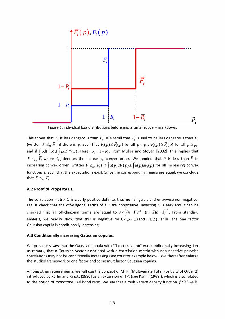
binary random variables and are plotted in Figure 1.

25

Figure 1. individual loss distributions before and after a recovery markdown.

This shows that iF is less dangerous than iF . We recall that iF is said to be less dangerous than iF (written i D iF F≤ ) if there is 0p such that ( ) ( )i iF p F p≤ for all 0p p< , ( ) ( )i iF p F p≥ for all 0p p≥

and if ( ) * ( )pdF p pdF p≤∫ ∫ . Here, 0 1 ip R= − . From Müller and Stoyan [2002], this implies that

i icx iF F≤ where icx≤ denotes the increasing convex order. We remind that iF is less than iF in

increasing convex order (written i icx iF F≤ ) if ( ) ( ) ( ) ( )i iu p dF p u p dF p≤∫ ∫ for all increasing convex

functions u such that the expectations exist. Since the corresponding means are equal, we conclude that i cx iF F≤ . A.2 Proof of Property I.1. The correlation matrix Σ is clearly positive definite, thus non singular, and entrywise non negative. Let us check that the off-diagonal terms of 1−Σ are nonpositive. Inverting Σ is easy and it can be

checked that all off-diagonal terms are equal to ( ) 12( 1) ( 2) 1n nρ ρ ρ−

× − − − − . From standard

analysis, we readily show that this is negative for 0 1ρ< < (and 2n ≥ ). Thus, the one factor Gaussian copula is conditionally increasing. A.3 Conditionally increasing Gaussian copulas. We previously saw that the Gaussian copula with “flat correlation” was conditionally increasing. Let us remark, that a Gaussian vector associated with a correlation matrix with non negative pairwise correlations may not be conditionally increasing (see counter-example below). We thereafter enlarge the studied framework to one factor and some multifactor Gaussian copulas. Among other requirements, we will use the concept of MTP2 (Multivariate Total Positivity of Order 2), introduced by Karlin and Rinott [1980] as an extension of TP2 (see Karlin [1968]), which is also related to the notion of monotone likelihood ratio. We say that a multivariate density function : df →

p

1

( ) ( ),i iF p F p

1 iP−

iF

iF

1 iP−

1 iR−1 iR−

26

is MTP2 if ( ) ( ) ( ) ( )f x f y f x y f x y≤ ∧ ∨ for all , dx y∈ 30. Let us notice that f is MTP2, if and only if

the log-density is supermodular: In the smooth case, we will only need to check that ( )2 ln

0i j

f xx x

∂≥

∂ ∂

for all i j≠ . If ( )1, , nV V is random vector with a MTP2 density, we say that ( )1, , nV V is MTP2. If

( )1, , nV V is MTP2, then ( )1, , nV V is conditionally increasing (Müller and Scarsini [2001], Theorem 3.3). In the case of Gaussian vectors, with invertible covariance matrices, the converse is true: if ( )1, , nV V is conditionally increasing, then ( )1, , nV V is MTP2 (Müller and Scarsini [2001], Theorem 3.6). As stated in the core text, an equivalent statement is that the inverse of the covariance matrix is a M - matrix (and necessarily pairwise correlations are non negative). Let us notice that in the general case, if a random vector is MTP2, it is conditionally increasing and the implication is strict. A.3.1 One factor Gaussian case. We do not assume here flat correlations. The Gaussian vector

( )1, , nV V can then be written 1i i i iV V Vρ ρ= + − , where 1, , , nV V V are independent standard Gaussian random variables and 0 1iρ< < , 1, ,i n= .

The conditional density of iV given V is such that ( )( )

( )( )

2

1 exp2 12 1

ii

ii

x vf x v

ρ

ρπ ρ

− = − −−

. It can

easily be checked that the corresponding latent variable model is latent TP2 as defined in Holland and

Rosenbaum [1986]: ' , 'x x u u∀ > ∀ > ( ) ( )( ) ( )

' '1

' 'i i

i i

f x v f x vf x v f x v

≥ . Using theorem 5 in the quoted paper, the

distribution of ( )1, , nV V is (conditionally) MTP2. Thus, the one factor Gaussian copula (with non flat correlations) is conditionally increasing. A.3.2 Multifactor Gaussian case. The multifactor case is more intricate: it might be reasonable to state that if all factor loadings are positive, then the corresponding Gaussian vector is conditionally increasing. Unfortunately, this may not be the case. Let us consider the following counter-example with three names:

2 21 1

2 22 2

2 23 3

0.1 0.9 1 0.1 0.9

0.7 0.3 1 0.7 0.3

0.9 0.1 1 0.9 0.1

V V W V

V V W V

V V W V

= × + × + − − × = × + × + − − ×

= × + × + − − ×

where 1 2 3, , , ,V W V V V are independent standard Gaussian variables. The covariance matrix of

( )1 2 3, ,V V V , Σ (respectively its inverse 1−Σ ) are given by:

1

1 .34 .18 1.14 .44 .09.34 1 .66 .44 1.95 1.20.18 .66 1 .09 1.20 1.78

−

− Σ = Σ = − − −

As a consequence, 1−Σ is not a M -matrix (some off-diagonal entries are positive) and ( )1 2 3, ,V V V is not conditionally increasing. Therefore, in factor models with positive factor loadings, the pairwise

30 If ( )1, , dx x x= , ( )1, , dy y y= , then x y∧ and x y∨ are defined by:

( ) ( )( )1 1min , , ,min ,d dx y x y x y∧ = , ( ) ( )( )1 1max , , ,max ,d dx y x y x y∨ = .

27

correlations are positive, but the copula is not always conditionally increasing, thus we cannot predict the effect of a recovery markdown. On theoretical and probabilistic grounds, in the case of Gaussian vectors, when all pairwise correlations are non-negative, the Gaussian vector is positively associated (see Pitt [1983], Joag-dev et al. [1983]) and the converse is obviously true. On the other hand, from Müller and Scarsini [2000] or Müller [2001], we know that a Gaussian vector is positive supermodular dependent (PSMD) if and only if all pairwise correlations are non-negative. As a consequence, in the case of multivariate Gaussian vectors, positive association and PSMD are equivalent and characterized by non-negativity of pairwise correlations. Let us notice that in the general case, if a random vector is positively associated, it is positive supermodular dependent and the implication is strict. In the Gaussian case MTP2 or CI imply positive association or PSMD and the implication is strict. A.3.3 Multifactor Gaussian case with inter and intrasector correlations. We consider thereafter a model with two layers that can deal with intra and intersector correlation (see Gregory and Laurent [2004]). Within each sector a one factor model applies, with a factor specific to the considered sector. The latent variable associated with name i can be written ( ) 1i i k i i iV W Vρ ρ= + − where ( )k i refers to the sector associated with name i . On top of that, the latent sector factors are related together through another one factor model, the latter factor being thus common to all names:

( ) ( ) ( ) ( )1k i k i k i k iW V Wβ β= + − .

The resulting correlation matrix is closely related to the class of intra-inter-class correlation matrices as defined by Eaton [1993]. Using linear algebra techniques, Kurata [2004] has shown that the inverses of such matrices are actually M - matrices. Thus, in their framework, ( )1, , nV V is conditionally increasing. However, when correlation parameters are name or sector dependent, we need to adapt the proofs. We will thereafter rely on a probabilistic approach, namely Theorem 7 of Holland and Rosenbaum [1986], which is derived from Proposition 3.4 of Karlin and Rinott [1980], in order to study the dependence properties of ( )1, , nV V :

(i) ( )1, , nV V is conditionally independent on the sector factors ( )k iW and thus the latent conditional independence property is fulfilled.

(ii) The conditional densities ( )i if x w of the iV ’s with respect to the vector of the sector

factors are MTP2 as functions of ( ),ix w : let us first notice that ( )i if x w only involves ix

and ( )k iw . Then, it is well-known (Karlin and Rinott [1980]) that if is MTP2 if if is TP2 for

every pair of variables, with other variables held fixed. As for the pair ( )( ),i k ix w , we only

need to duplicate the proof of latent TP2 already written above in the one factor Gaussian case. As for the other pairs, the result is also straightforward, since the involved ratio is equal to one.

(iii) Using the previous analysis of the one factor Gaussian case, the random vector whose components are the sector factors ( )k iW , is MTP2.

This shows that ( )1, , nV V is MTP2 (and thus conditionally increasing). A.4 Proof of Property I.2.

28

Let us first note that ( )1, , nV V and ( )1, , nV V− − share the same joint distribution and thus the same

conditionally increasing copula. Since individual losses ( ) ( ){ }11 1i i

i V PR −≤Φ

− , ( ) ( ){ }11 1i i

i V PR −≤Φ

− are non

decreasing functions of iV− , the random vectors ( ) ( ){ } ( ) ( ){ }1 11 1

11 1 , , 1 1n n

nV P V PR R− −≤Φ ≤Φ

− −

and

( ) ( ){ } ( ) ( ){ }1 11 1

11 1 , , 1 1n n

nV P V PR R− −≤Φ ≤Φ

− −

share the same conditionally increasing (one factor

Gaussian) copula. Moreover, since for all 1, ,i n= , ( ) ( ){ } ( ) ( ){ }1 11 1 1 1i i i i

i cx iV P V PR R− −≤Φ ≤Φ

− ≤ − , we

conclude that:

( ) ( ){ } ( ) ( ){ } ( ) ( ){ } ( ) ( ){ }1 1 1 11 1 1 1

1 11 1 , , 1 1 1 1 , , 1 1n n n n

n dcx nV P V P V P V PR R R R− − − −≤Φ ≤Φ ≤Φ ≤Φ

− − ≤ − −

.

Then, the portfolio losses can be compared through the convex order: ( ) ( ){ } ( ) ( ){ } ( ) ( ){ } ( ) ( ){ }1 1 1 1

1 1 1 11 11 1 1 1 1 1 1 1

n n n nn cx nV P V P V P V P

R R R R− − − −≤Φ ≤Φ ≤Φ ≤Φ− + + − ≤ − + + − ,

since for any convex function :g → , ( ) ( )1 1, , n nf x x g x x= + + is directionally convex. This leads to the stated result on the expected loss on CDO tranches given the convexity (resp. concavity) of senior (resp. equity) tranche payoffs with respect to the portfolio loss. A.5 Empirical investigation of a recovery markdown. To make the theoretical results of the previous subsection more tangible, we examine here the practical case of the DJITX S9 MST index on January 2009, 5th. The corresponding 5Y tranche quotes are displayed in Table 7.

Table 7: 5Y DJITX S9 MST tranche quotes for an index reference spread of 180 bps on January 2009, 5th. The equity tranche is quoted in an upfront payment while the others are quoted in running

spreads.

To estimate the impact of a recovery markdown, we first computed expected tranche losses at a given maturity for two correlation levels – the spreads of the portfolio constituents being adjusted to the reference quoted spread31. The results are shown in Tables 8 and 9. As predicted by Property I.2, the expected losses on equity tranches are increasing with the recovery rate.

31 Let us note that all individual spreads have been matched to CDS quotes. However, there is some discrepancy between the Index spread and the average CDS spread of the names within the index. This basis effect is reported for example in Beinstein [2009]. To cope with this, we used some multiplicative adjustment on individual credit spreads. This guarantees consistency of the individual credit spreads with the index quote. In the modelling field, Eckner [2007] or Herbertsson [2008] deal with similar issues.

Attachment Point

Detachment Point Upfront Mid Mid Running Spread

0.0 % 3.0 % 68.50 % (68.00 ; 69.00) % 500 (500 ; 500) 3.0 % 6.0 % 1,245 (1,230 ; 1,260) 6.0 % 9.0 % 620 (610 ; 630) 9.0 % 12.0 % 360.5 (353 ; 368)

12.0 % 22.0 % 110 (106 ; 113)

29

Recovery [0 , 3] % [0 , 6] % [0 , 9] % [0 , 12] % [0 , 22] % [0 , 100] % 0 % 1.983 % 3.061 % 3.697 % 4.091 % 4.642 % 4.838 % 5 % 2.009 % 3.093 % 3.729 % 4.119 % 4.658 % 4.838 %

10 % 2.029 % 3.124 % 3.761 % 4.149 % 4.674 % 4.838 % 15 % 2.051 % 3.159 % 3.797 % 4.181 % 4.691 % 4.838 % 20 % 2.077 % 3.195 % 3.835 % 4.215 % 4.707 % 4.838 % 25 % 2.109 % 3.237 % 3.876 % 4.252 % 4.724 % 4.838 % 30 % 2.135 % 3.278 % 3.918 % 4.289 % 4.740 % 4.838 % 35 % 2.168 % 3.324 % 3.964 % 4.330 % 4.757 % 4.838 %

Table 8: DJITX S9 MST expected tranche losses expiring on the 20th of June 2011, computed for different assumptions of recovery rate and a correlation of 30 %.

Recovery [0 , 3] % [0 , 6] % [0 , 9] % [0 , 12] % [0 , 22] % [0 , 100] %

0 % 1.377 % 2.165 % 2.712 % 3.121 % 3.948 % 4.838 % 5 % 1.405 % 2.203 % 2.756 % 3.167 % 3.993 % 4.838 %

10 % 1.431 % 2.242 % 2.802 % 3.216 % 4.040 % 4.838 % 15 % 1.460 % 2.286 % 2.852 % 3.268 % 4.089 % 4.838 % 20 % 1.492 % 2.332 % 2.906 % 3.325 % 4.141 % 4.838 % 25 % 1.530 % 2.384 % 2.964 % 3.386 % 4.196 % 4.838 % 30 % 1.566 % 2.439 % 3.027 % 3.451 % 4.253 % 4.838 % 35 % 1.608 % 2.500 % 3.096 % 3.523 % 4.314 % 4.838 %

Table 9: DJITX S9 MST expected tranche losses expiring on the 20th of June 2011, computed for different assumptions of recovery rate and a correlation of 60 %.

Another way of quantifying the impact of a recovery markdown is to consider the base correlation skews resulting from the calibrations to the tranche quotes of Table 7 for different recovery assumptions. The expected pattern is clear using Property I.2 since equity tranche prices are decreasing with correlation: a decrease of the recovery rate will give rise to a decrease of the base correlations. The results of Table 10 confirm this assessment. We also note that the base correlation skews tend to flatten as the recovery decreases. The intuition behind this is rather straightforward since it becomes much easier to reach large losses under a low recovery rate assumption and one does not need to use high correlation levels to cope with these fat tail effects. This flattening of base correlations is a desirable feature. In a well specified model, implied parameters should not depend upon the priced tranche. On more practical grounds, this eases the computation of tranchelets and bespoke tranches by numerical interpolation or other “mapping” techniques and solves pathologies such as negative spread deltas.

Recovery [0 , 3] % [0 , 6] % [0 , 9] % [0 , 12] % [0 , 22] % 0 % 28.69 % 36.50 % 42.51 % 47.97 % 68.67 % 5 % 29.85 % 37.67 % 43.78 % 49.37 % 70.63 %

10 % 30.84 % 38.86 % 45.15 % 50.92 % 72.78 % 15 % 31.94 % 40.26 % 46.72 % 52.67 % 75.16 % 20 % 33.31 % 41.78 % 48.49 % 54.64 % 77.83 % 25 % 35.02 % 43.59 % 50.49 % 56.88 % 80.82 % 30 % 36.59 % 45.55 % 52.77 % 59.42 % 84.19 % 35 % 38.67 % 47.90 % 55.43 % 62.40 % 88.03 %

Table 10: 5Y DJITX S9 MST base correlation skews for different recovery rates.

30

A.6 Recovery markdown with Archimedean copulas. We rely on a result of Müller and Scarsini [2005]. They characterize the dependence structure of an Archimedean copula through some simple to check properties of its generator. Among other positive dependence concepts such as conditional increase in sequence and MTP2, they consider the case of conditional increase. We recall that a copula C is called Archimedean with generator ψ if it has the form:

( ) ( )11

1, ,

n

n ii

C u u uψ ψ −

=

=

∑ ,

where [ ]: 0,1ψ + → is a d -alternating function with ( )0 1ψ = and lim ( ) 0u

uψ→∞

= . ψ is said to be d

-alternating if ( ) ( )1 0k kψ− ≥ for { }1, ,k d∈ . In Theorem 2.8, Müller and Scarsini [2005] show that

C is conditionally increasing if and only if ( ) ( )1 ( 1)1 .n nψ− −− is log-convex. In the Clayton copula case,

we have ( ) ( ) 1/1u u θψ −= + . The positive dependence case is associated with 0θ > . Given that, we can easily check that the above assumption is fulfilled. On the other hand, we recall that the comparison between individual losses still holds since it only involves marginal distributions of individual losses and not the dependence structure. The same reasoning as for the one factor Gaussian copula case thus applies: the expected loss on a senior tranche increases after a recovery markdown while the converse applies to equity tranches when one considers a Clayton copula with positive dependence. A.7 Recovery markdown in the latent factor framework. The aim here is to show that the results stated for the Gaussian copula readily extends to a much wider class of latent factor models that encompasses most of credit models. Let us first introduce a rather general notion of factor models. Definition: Let us consider a set of default times ( )1, , nτ τ and a given time horizon t . We say that the default indicators { }1

i tτ ≤ , 1, ,i n= admit the monotone unidimensional representation if there

exists a random variable V such that: (i) The default indicators are conditionally independent given V . (ii) ( )i t Vτ > is non decreasing in V for all { }1, ,i n∈ .

This corresponds to models studied in Holland and Rosenbaum [1986] and Holland [1981]. They are also related to item response theory models with dichotomous responses in psychometrics. Let us notice that by considering V− instead of V , we can replace “non decreasing” by “non increasing” in (ii). From Holland [1981], Theorem 3, in the previous framework, default indicators exhibit a strong form of multivariate positive dependence, named MTP2. Holland and Rosenbaum [1986] even show a stronger form of dependence, named CMTP2. Based on earlier results by Karlin and Rinott [1980], Müller and Scarsini [2001], Theorem 3.3 show that MTP2 is a stronger form of positive dependence that conditional increase. As a consequence, whenever the default indicators admit the monotone unidimensional representation for all time horizons t , the result already stated in the Gaussian copula case applies: a recovery markdown leads to an increase of the risk of the credit portfolio (with

31

respect to the convex order) and subsequently an increase of the expected loss on senior tranches and a decrease of the expected loss on equity tranches. Let us now relate this with the analysis already done in the Archimedean copula framework. We recall that a function ψ is said to be completely monotone if it is d -alternating for any d ∈ . From Kimberling [1974], the generator ψ defines an Archimedean copula in any dimension if and only if it is a completely monotone function, or equivalently, a Laplace transform of a non-negative random variable. On practical grounds, this is a weak statement, since it means that the dependence structure can be extended to an arbitrary number of creditors. In that framework, Marshall and Olkin [1988] have provided a well-known sampling procedure that makes clear the underlying univariate latent structure: let 1, , ,nU U V be independent random variables, 1, , nU U being uniform on

( )0,1 , and V being a positive random variable with Laplace transform ψ . Then the joint distribution

of the random variables ln i

iUV

Vψ

− =

, 1, ,i n= is the Archimedean copula with generator ψ .

This also corresponds to the well-known framework of frailty models. Given marginal distribution function of default times, 1, , nF F , we can construct default times as ( )1

i i iF Vτ −= , 1, ,i n= , which do admit an Archimedean copula with generator ψ . Clearly, default times are independent

given V and ( ) ( )( )i i it V V F t Vτ > = > . Since ψ is decreasing, we get

( ) ( )( )( )11 expi it V V F tτ ψ −> = − − which is increasing in V . Thus, all frailty models are associated

with the monotone unidimensional representation for all time horizons, and the corresponding default indicators are associated with conditional increasing copulas. As discussed above, most well known Archimedean models are frailty models and thus admit the monotone unidimensional representation. For a discussion of sampling Archimedean copulas in a larger framework, we report to McNeil and Neslehova [2008]. Similarly, it is straightforward to check that additive factor copulas as defined in Cousin and Laurent [2008a] lead to default indicators belonging to the family of unidimensional monotone latent variable models. We refer to Cousin and Laurent [2008b] and the references therein for an extensive review of such models in a credit context. From the conditional default probability stated in Cousin and Laurent [2008b], it is also straightforward to check that the generic one-factor model Lévy model of Albrecher et al. [2007] is associated with the monotone unidimensional representation for all time horizons. As for the univariate case of the random factor loading model of Andersen and Sidenius [2005], using the same notations as theirs and defining the factor as ( )iV a Z Z= , we readily see that the default indicators once again exhibit the monotone unidimensional representation for all time horizons. This is also the case of the multivariate Poisson model and the affine intensity model described in the above review paper. The latter examples also show that the confrontation between copula models and other approaches is somehow sophistry, since these factor models are associated with the same kind of numerical implementation and dependence properties. Appendix B: Behaviour of loss given default. We state here some useful properties of the stochastic recovery rate in the Gaussian copula framework. The same also apply to frailty models, such as the Clayton copula, which was discussed in the core text. In the latter case, the proofs are straightforward and do need not to be detailed. Property II.1 (bounds on loss given default):

1) ( ) min0 1 iiM V R≤ ≤ − , for all V ∈ .

32

2) Let us assume that 0ρ > . Then, ( )lim 0V iM V→∞ = and ( ) minlim 1 iV iM V R→−∞ = − .

Proof of Property II.1: Let us first show statement 1. Since ( )0 iM V≤ and i iP P≤ ,

( ) ( )1 1

1 1i iP V P Vρ ρ

ρ ρ

− −Φ − Φ −≤

− − for all V since 1−Φ is increasing. Since Φ is also increasing,

( ) ( )1 1

01 1i iP V P Vρ ρ

ρ ρ

− − Φ − Φ − < Φ ≤ Φ − −

, which yields:

( ) min1 iiM V R≤ − .

Let us now check that the bounds are strict. ( ) minlim 1 iV iM V R→−∞ = − is obvious. ( )lim 0V iM V→∞ =

can be proven using l’Hôpital’s rule. Corollary II.1 (bounds on recovery rates): let us denote by ( ) ( )1i ir V M V= − the recovery rate. Then,

( )min 1iiR r V≤ ≤ and the bounds are strict.

Property II.2 (Monotonicity of loss given default wrt V ): Let us assume that, 0 1iP< < ,

min0 1iiR R≤ ≤ ≤ and 0ρ > . Then, ( )iV M V→ is decreasing.

Proof of Property II.2:

( ) ( )

( )

( )( )

( ) ( ) ( )

( )

1 1 1 1

min min1 1

1 1 11 1

1 1

i i i i

i ii

i i

P V P P P V

M V R RP V P V

ρ ρρ ρ ρ

ρ ρρ ρ

− − − −

− −

Φ − Φ −Φ Φ − Φ Φ + − − − = − = − Φ − Φ −

Φ Φ − −

.

Let us denote by ( ) ( )1 1

01

i iP Pa

ρ

− −Φ −Φ= >

− and by

( )1

1iP V

xρ

ρ

−Φ −=

−. Then, we need to check that

( )( )

x ax

xΦ −

→Φ

is increasing. Thus, we need to check that ( ) ( ) ( ) ( )' ' 0x a x x a xΦ − Φ −Φ − Φ > for all

x . For simplicity, we scale Φ to 2

( )x

ux e du−

−∞

Φ = ∫ . Since 2

( )x a

ux a e du−

−

−∞

Φ − = ∫ , setting v u a= + , we

get, ( ) ( )2x

v ax a e dv− −

−∞

Φ − = ∫ . We have to check that ( )( )2 2 2 2( ) 0x

x a u u a xe e e e du− − − − − −

−∞

− >∫ . The integrand

can be written as ( )2 2 2( ) 2 2 0x a u ax aue e e− + + − > . This completes the proof.

Negative “correlation” between default indicators and losses given default. We will show that any default indicator

( ){ }11i iV P−≤Φ

is negatively associated with any loss given default ( )jM V . Two random

variables ,X Y are said to be negatively associated if ( ) ( )( ), 0Cov f X g Y ≤ for all non decreasing functions ,f g such that the above covariance exists. By conditioning on V and rearranging terms, it can be readily checked that:

( ){ } ( )( ) ( ) ( ) ( )( )( )11 , (1) (0) , 0i i

j i jV PCov f g M V Cov f f P V g M V−≤Φ

= − ≤ .

33

The latter inequality comes from the fact that ( ) ( )(1) (0) if f P V− and ( )( )jg M V are counter

monotonic and can be proven using a result due to Hoeffding [1940] which states that for non negative random variables ,X Y , with joint distribution function ,X YF and marginal distribution functions ,X YF F , we have:

( ) ( ) ( ) ( )( ),0 0

, ,X Y X YCov X Y F u v F u F v dudv∞ ∞

= −∫ ∫ .

The reader is referred to Dhaene and Goovaerts [2005] for details of the proof. For counter

monotonic variables, we have ( ) ( ), , ( ) ( ) 1X Y X YF u v F u F v += + − , which corresponds to the lower

Hoeffding-Fréchet bound and ( )( ) ( ) 1 ( ) ( )X Y X YF u F v F u F v++ − ≤ (see Embrechts et al. [2002] for more details), from which we deduce the stated inequality. As a consequence, default indicators and losses given default also exhibit negative dependence with respect to the supermodular order (see Christofides and Vaggelatou [2004]). Appendix C: Proofs of section III. C.1 Dynamics of portfolio loss: time to recovery and spot recovery. Since CDO tranche pricing only involve a series of single horizon pricing problems, we do not need to be concerned with the extension of the model to several times horizon. Let us however discuss a few points associated with the trajectories of the portfolio loss if one were to adopt a copula of default times approach (say because one wishes to implement tranche pricing as a Monte Carlo on default

times). The portfolio loss ( ) ( ){ }1

11

i i

n

i V Pi

L M V −≤Φ=

=∑ jumps at default times iτ , { }1, ,i n∈ by a

magnitude of ( )iM V which depends upon the default date due to the time dependency in the loss

given default ( )iM V (it involves marginal default probabilities ( )i iP F t= up to the current date). After name i (say) has defaulted and before the next default occurs, the portfolio loss is not constant as one could have expected, due to the previous time dependence effect. We may also notice that the perfect dependence of recovery rates with respect to the underlying factor is not innocuous. At the first default, one knows the magnitude of the jump in the loss process and therefore the value of V (we recall that ( )iM V is monotonic in V ). Thus, subsequently, recovery rates are perfectly known. All this points to the fact that this model has been optimized for single period use and that a naive extension of this stochastic recovery model in a default time copula framework has not been intended. The previous approach is known as the recovery to maturity model. To circumvent the issues associated with the dynamics of the portfolio loss, Bennani and Maetz [2009], Li [2009] have considered a spot recovery approach. In the latter framework, the portfolio loss jumps by a magnitude of ( ),i im Vτ at default time iτ and remains constant between two default

times. Using the same notations as in the core text and since ( )( )1i i iF Vτ −= Φ , we write (with a slight

abuse of notation), the individual loss on name i at time t as ( ) ( ){ }1 ( ), 1

i ii i V F t

m V V −≤Φ to be compared

with the above ( ) ( ){ }11i i

i V PM V −≤Φ

(the dependence in t being implicit for notational simplicity).

Consistency with the value of credit default swap implies: ( ) ( ){ } ( ) ( )1 ( ), 1 1

i ii i i iV F t

E m V V R F t−≤Φ = −

.

This is sometimes stated equivalently as ( ) ( ) ( )1, ( ) 1i i i i iE m V V V F t R− ≤ Φ = − .

34

Let us denote by ( ) ( ),i i i ig V E m V V V = . From the law of iterated expectations,

( ) ( ){ } ( ) ( ){ }1 1( ) ( )1 1 1

i i i ii i iV F t V F t

E g V E R− −≤Φ ≤Φ = −

. Assuming a smooth marginal distribution of iτ and

differentiating with respect to t leads to: ( ) ( ), 1i i i i iE m V V V g V R = = − . Let us now define

1i

iV V

Zρ

ρ−

=−

, thus: ( ) ( ), , 1i i i i i im V V m V V Zρ ρ= − − . Let us note that ( ),i iV Z is a Gaussian

vector with independent components. As a consequence:

( ) ( ), 1 , 1 1i i i i i i i iE m V V Z V v E m v v Z Rρ ρ ρ ρ − − = = − − = − .

This constrains the range of consistent specifications of spot recovery rates. The easiest way to cope with the above equation is to assume, as in Bennani and Maetz [2009], that the spot recovery rate only depends upon iZ . However, as a consequence, for a given name, spot recovery rate and default time are independent. This may look as an undesirable feature on economic grounds. C.2 Proof of property III.1. Let us denote by ( ) ( ){ }11

i ii i V P

Z M V −≤Φ= , the loss associated with name i . Then:

( ) ( ) ( ) ( )11

min11 1

ii ii i

P VP VE Z V M V R

ρρρ ρ

−− Φ −Φ − = Φ = − Φ − −

.

Then, ( ) ( )1

min1 1

11

n nii

LP ii i

P VL R E Z V

ρ

ρ

−

= =

Φ − = − Φ = −

∑ ∑ .

We recall a result from Dhaene et al. [2002]. Let ( )1, , nZ Z Z= be a random vector and V a random variable. Then:

1 1n cx nE Z V E Z V Z Z + ≤ + + ,

where cx≤ is the convex order. This readily shows the stated property. C.3 Proof of Property III.2.

For simplicity, we denote the conditional default probabilities by ( ) ( )1

1i

i

P VP V

ρρ

− Φ −= Φ −

and

( ) ( )1

1i

i

P VP V

ρ

ρ

− Φ − = Φ −

.

We readily have:

( ) ( ){ } ( ) ( ) ( )( )

( ) ( ){ } ( ) ( )( ) ( )( )

1

1

2

min min

22

min

1 1 1 1

1 1 1

i i

i i

i ii iV P

iii iV P

i

Var R V R P V P V

P VVar M V V R P V

P V

−

−

≤Φ

≤Φ

− = − −

= − −

,

for { }1, ,i n∈ . As a consequence, in order to compare the conditional variances, we just need to

compare ( )

( )1 i

i

P VP V−

and ( )

( )1 i

i

P VP V−

. This is straightforward since ( )iP V is increasing in iP . Thus,

35

( )( )

1 i

i

P VP V−

is decreasing in iP . On the other hand, i i iP wP P= ≥ . Thus, ( )

( )( )

( )1 1

,i i

i i

P V P VV

P V P V− −

≤ ∀ ∈

which shows the stated property. C.4 Expansions around the Poisson distribution. Orthogonal polynomials associated to the Poisson probability mass function defined, for a fixed

0λ > and j∈ , by: { }( ) ( )exp!

j

p jjλλ λ= − , are known as the Charlier polynomials and are defined

by (see Szegö [1975]): ( ) ( ) ( )0

!k

ik

i

k xx C x i

i iλ λ −

=

→ = −

∑ . An expansion can be derived for the

(pseudo-) distribution of a (rescaled) loss defined by ( ) ( )LL S V

M V= + :

{ }( ) ( ) { }( ) ( ) ( ) ( )( ) ( )2

1!

Pkn

Vk kV

k

Vj p j P V C j

kλ

λ

λµ

=

= +

∑ (2)

where ( )V E L Vλ = is the mean of the rescaled loss, ( ) ( )( ) ( )Vk kP V E C L Vλ = allows us to fit the

thk conditional moment of the rescaled loss and Pn ( 1≥ ) is the number of matched moments. In the above expansion, we voluntarily did not specify the values of the rescaling factors ( )M V and ( )S V as Pn conditional moments of the loss are matched whatever their values32. C.5 Expansions around the binomial distribution. In the case of a binomial distribution, whose mass probability function is defined, for fixed ( )0,1p∈ and 1n > , by:

{ }( ) ( ), 1 n jjp n

nb j p p

j−

= −

,

32 For the numerical results, which are displayed subsequently, we did the following choices. First,

the scaling factor is taken equal to the average loss given default: ( ) ( )1

1 n

ii

M V M Vn =

= ∑ , so that

( )L S V− takes integer values when all ( )iM V are the same. Second, the shifting factor ( )S V is chosen in order to prepare the rescaled loss distribution for a Poisson approximation:

( ) ( ) ( )2 1E L V Var L V

S VM V M V

= − +

, where . denotes the floor function. Indeed, with this

specification, L satisfies: 1Var L V E L V − ≤ whereas for a true Poisson distribution, we

would have equality of mean and variance. Finally, a last trick consists in approximating, with the

above expansion, the « mirror » of the portfolio loss ( )1

n

ii

M V L=

−

∑ instead of the loss itself, when

( )1

12

n

ii

E L V M V=

> ∑ , to minimize the probability of the approximated loss to be greater than its

theoretical maximum value.

36

for 0, ,j n= , the relevant polynomials are the Krawtchouk polynomials defined by:

( ) ( ) ( ) ( ),

01

ki k ip n

ki

x n xx K x p p

i k i−

=

− → = − − −

∑ (see Szegö [1975]), where n is the number of portfolio

constituents. We rescale the portfolio loss by the average loss given default ( ) ( )1

1 n

ii

M V M Vn =

= ∑

and approximate the distribution of the rescaled loss ( )LL

M V= by:

{ }( ) ( ) { }( ) ( )( ) { }( )

( )( ) ( ),,

2 ,

1Bn

p V nkkp V n

k p V n

B Vj b j K j

b kν

=

= +

∑ ,

where ( )p V E L V = is the mean of the rescaled loss, ( ) ( )( ) ( ),p V nk kB V E K L V = allows us to fit

the thk conditional moment of the rescaled loss and Bn ( 1≥ ) is the number of matched moments. Appendix D: Proofs of section IV. D.1 Proof of Property IV.1. Clearly, ( )iM V is not defined for 100%ρ = . We may think of considering ( )

1lim iM Vρ→

. Formally, this

leads to ( ) ( ){ }

( ){ }

1

1

min

11

1i

i

V Pi

V P

R−

−

<Φ

<Φ

− . Keeping in mind that ( ) ( )1 1i iP P− −Φ ≤ Φ , we have ( ) min1

lim 1 iiM V R

ρ→= −

(the recovery rate is then equal to miniR ) for ( )1

iV P−< Φ , ( )1

lim 0iM Vρ→

= for ( ) ( )1 1i iP V P− −Φ ≤ < Φ

(the recovery rate is then equal to one). Dealing rigorously with the indeterminacy for ( )1iV P−≥ Φ is

cumbersome, but this is not useful either as discussed now. We recall that the portfolio loss is

provided by ( ) ( ){ }1

11

i i

n

i V Pi

L M V −≤Φ=

=∑ . We will now consider the limits ( ) ( ){ }11

lim 1i i

i V PM V

ρ−≤Φ→

.

( ) ( ){ }11i i

i V PM V −≤Φ

can be written as: ( ) ( ){ }

( )( )1

1

min 1

11

11

i iV P ii

i

P VR

P V

ρ

ρρρ

−−

≤Φ

−

Φ − − ×Φ −Φ − Φ −

.

It can easily be checked that ( ){ }

( )1

11

1lim 0

1

i iV P

iP Vρ ρρ

−≤Φ

−→=

Φ −Φ −

on ( ){ }1iV P−> Φ and

( ){ }

( )1

11

1lim 1

1

i iV P

iP Vρ ρρ

−≤Φ

−→=

Φ −Φ −

on ( ){ }1iV P−< Φ . As a consequence

( ){ }

( )1

1

1

1

i iV P

iP Vρρ

−≤Φ

− Φ −Φ −

converges

almost surely to ( ){ }11

iV P−≤Φ as 100%ρ → . Since meanwhile

( )1

1iP Vρ

ρ

− Φ − Φ −

converges to

( ){ }11iV P−<Φ

as 1ρ → , we conclude that the loss associated with name i converges almost surely to

( ) ( ){ }1min1 1i

iV P

R −≤Φ− .

37

Since all individual losses are bounded by zero and one, we conclude that the expected tranche losses and the corresponding up-front or running premiums converge accordingly using Lebesgue’s theorem. D.2 Proof of Property IV.2. First, let us show that:

( ){ } ( ) ( ){ }1 1min( )1 1 1i i i

ii cxV P V P

M V R− −≤Φ ≤Φ≤ − .

In subsection III.5, it was proven that ( ) ( ){ } ( ) ( ){ }1 1min1 1 1i i i i

V ii cxV P V P

M V R− −≤Φ ≤Φ≤ − , which implies the

unconditional convex order: ( ) ( ){ } ( ) ( ){ }1 1min1 1 1i i i i

ii cxV P V P

M V R− −≤Φ ≤Φ≤ − . Since convex ordering only

involves the marginal distributions of left and right hand terms and since iV and V share the same distribution, we deduce the stated inequality between individual losses. Let us now consider some one dimensional distribution functions 1, , nF F and * *

1 , , nF F such that *

i cx iF F≤ , 1 i n≤ ≤ . Ky Fan – Lorentz theorem states that:

( ) ( )( ) ( ) ( )( )1 1 * 1 * 11 1, , , ,n dcx nF U F U F U F U− − − −≤ ,

where U is uniformly distributed on ( )0,1 . In the following, for 1 i n≤ ≤ , iF denotes the marginal distribution function of

( ){ }1( )1i i

i V PM V −≤Φ

and

*iF is the marginal distribution function of ( ) ( ){ }1min1 1

i

iV P

R −≤Φ− . Lorentz theorem (see Tchen [1980])

states that: ( ) ( )( ) ( ) ( )( )1 11 1 1, , , ,n n sm nM V I M V I F U F U− −≤ . Using the transitivity of the

directionally convex order, we get:

( ) ( )( ) ( ) ( ){ } ( ) ( ){ }1 11

11 1 min min, , 1 1 , , 1 1

n

nn n dcx V P V P

M V I M V I R R− −≤Φ ≤Φ ≤ − −

.

We conclude that: ( ) ( ) ( ) ( ){ } ( ) ( ){ }1 1

1

11 1 min min1 1 1 1

n

nn n cx V P V P

M V I M V I R R− −≤Φ ≤Φ+ + ≤ − + + −

Thus, the loss associated with 100%ρ = is always greater with respect to the convex order than the actual loss in the stochastic recovery model. As a consequence,

( ){ } ( ) ( ){ }1 1min1 1

1 1( ) 1 1 1i i i

n ni

i V P V Pi i

E M V K E R Kn n− −

+ +

≤Φ ≤Φ= =

× − ≤ − −

∑ ∑ for all 0 1K≤ ≤ .

D.3 Proof of Lemma IV.1. Let us denote by iF the distribution function associated with ( ) ( ){ }11 1

i ii V P

R −≤Φ− and by iF the

distribution function associated with ( ) ( ){ }11i i

i V PM V −≤Φ

. We will show that i D iF F≤ . First:

( ) ( ){ } ( ){ } ( ) ( )1 1 min1 1 ( )1 1 1i i i i

ii i i i iV P V P

E R E M V R P R P− −≤Φ ≤Φ − = = − = −

.

38

We can also notice that the distribution function of the binary random variable ( ) ( ){ }11 1i i

i V PR −≤Φ

− is

piecewise constant as studied above in the perfect correlation case for the random variable ( ) ( ){ }1min1 1

V PR −≤Φ

− .

( ) ( ){ }11

i ii V P

M V −≤Φ has a probability mass at zero:

( ) ( ){ } ( ){ }1 11 0 1 0 1i i i i

i iV P V PM V P− −≤Φ ≤Φ = = = = −

.

Figure 2. Comparison of individual name loss distributions in the case of fixed recovery rate and no correlation and of stochastic recovery rate

Figure 2 plots iF and iF . We readily see that *

i D i D iF F F≤ ≤ , which shows the lemma. D.4 Proof of Lemma IV.2 We need first to state and prove the following: If ,X Y are two square integrable random variables independent upon some random vector V 33, then:

( ) ( ), ,Cov X Y Cov E X V E Y V = .

Indeed, ( ) [ ] [ ] [ ],Cov X Y E XY E X E Y E E XY V E E X V E E Y V = − × = − × , using the

law of iterated expectations. E XY V E X V E Y V = × , due to the conditional independence of ,X Y upon V , which shows the previous equality.

33 The conditional independence can be defined in slightly different ways. Here, we say that ,X Y are

conditionally independent upon V if ( ) ( ) ( ) ( )E h X g Y V E h X V E g Y V = × for all measurable functions ,h g such that the expectations are well-defined.

pmin1 iR−

1

( ) ( ) ( ){ }( )1*

min1 1i

ii V P

F p Q R p−≤Φ= − ≤

1 iP−

iF*

iF

1 iP−

1 iR−

( ) ( )( )i i iF p Q M V I p= ≤

( ) ( ) ( ){ }( )11 1i i

i i V PF p Q R p−≤Φ

= − ≤

iF

39

We now proceed to the proof of Lemma IV.2. Here ( ) ( ){ } ( )11

1 ,i i

i i iV V PX M V l V V

ρ ρ −+ − ≤Φ= = . Since

( ) ( )( )( 1) 1, , , ,i i nX l V V l V V+ += , { }1iX t> and ( )( 1)if X + are conditionally independent upon V . As a

consequence of the previous lemma,

{ } ( )( ) { } ( )( )( 1) ( 1)1 , 1 ,i ii iX t X tCov f X Cov E V E f X V+ +> >

= .

Since ( )iM V and ( ){ }11

1i iV V Pρ ρ −+ − ≤Φ

are non negative and non increasing in V , ( ), il V V is also non

increasing in V for any given value of iV . The same applies to { } ( ){ },1 1

i iX t l V V t> >= . Thus

{ } ( ){ } ( ),1 1i iX t Vl v z tE V v dz> >

= = ∫ , where iV is the distribution of iV , is a non increasing function

of v . The same line of reasoning applies to ( )( 1)iE f X V v+ = . As a consequence,

{ } ( )( )( 1)1 , 0i iX tCov E V E f X V+>

≥ , which shows the stated result.

D.5 Proof of Property IV.3. We first show that:

( ) ( ){ } ( ) ( ){ } ( ) ( ){ } ( ) ( ){ }1 1 1 11 1 1 1

1 11 1 , , 1 1 1 , , 1n n n n

n wcs nV P V P V P V PR R M V M V− − − −≤Φ ≤Φ ≤Φ ≤Φ

− − ≤

,

where wcs≤ stands for the weakly conditional increase in sequence order. Since the right hand term is made of independent components, the above inequality holds if

( ) ( ){ } ( ) ( ){ }1 11 1

1 1 , , 1n n

nV P V PM V M V− −≤Φ ≤Φ

is weakly associated in sequence, which is actually the case,

using the previous lemma. We can now use Theorem 3.1 in Rüschendorf [2004]. We recall that this theorem states that given two random vectors, ( )1, , nX X X= and ( )1, , nY Y Y= , if i cx iX Y≤ for 1 i n≤ ≤ and wcsX Y≤ , then dcxX Y≤ . As a consequence,

( ) ( ){ } ( ) ( ){ } ( ) ( ){ } ( ) ( ){ }1 1 1 11 1 1 1

1 11 1 , , 1 1 1 , , 1n n n n

n dcx nV P V P V P V PR R M V M V− − − −≤Φ ≤Φ ≤Φ ≤Φ

− − ≤

.

We conclude that: ( ) ( ){ } ( ) ( ){ } ( ) ( ){ } ( ) ( ){ }1 1 1 1

1 1 1 11 11 1 1 1 1 1

n n n nn cx nV P V P V P V P

R R M V M V− − − −≤Φ ≤Φ ≤Φ ≤Φ− + + − ≤ + + ,

since for any convex function :g → , ( ) ( )1 1, , n nf x x g x x= + + is directionally convex.