Pricing basket options with an eye on swaptions

Pricing basket options

with an eye on swaptions

Alexandre d’Aspremont

ORFE

Part of thesis supervised by Nicole El Karoui.

Data from BNP-Paribas, London.

A. d’Aspremont, ORFE ORF557, stochastic analysis seminar, BCF, Sep. 2004. 1

Introduction

Why baskets, swaptions, calibration?

Interest rate derivatives trading

• Focus on structured products activity

• Discuss stability, speed and robustness

• few stable methods for model calibration and risk-management

• How do we extract correlation information from market option prices?


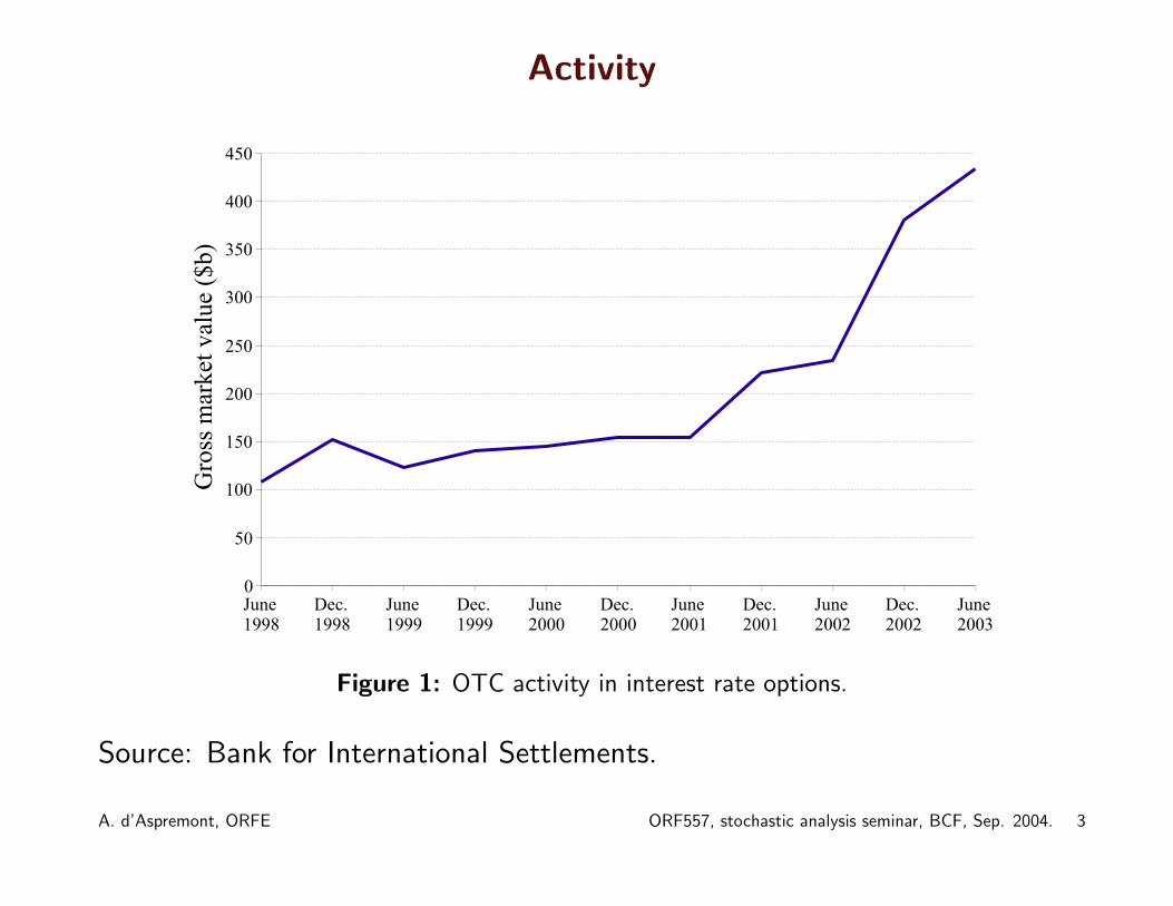
Activity

Figure 1: OTC activity in interest rate options.

Source: Bank for International Settlements.


Structured Interest Rate Products

Structured derivatives desks act as risk brokers

• buy/sell tailor made products from/to their clients

• hedge the resulting risk using simple options in the market

• manage the residual risk on the entire portfolio

P&L comes from a mix of flow and arbitrage. . .


Derivatives Production Cycle

market data

⇓

model calibration

⇓

pricing & hedging

⇓

risk-management


Derivatives Production Cycle, Trouble. . .

market data: illiquidity, Balkanization of the data sources

⇓

model calibration: inverse problem, numerically hard

⇓

pricing & hedging: American option pricing in dim. ≥ 2

⇓

risk-management: all of the above. . .


Objective

• However, it works

• Numerical difficulties creates P&L hikes, poor risk description, . . .

• Our objective here: improve stability, robustness

• Focus first on calibration

• Using new cone programming techniques to calibrate models and manageportfolio risk


Outline

• Pricing baskets

• Application to swaptions

• Cone programming, a brief introduction (next talk)

• IR model calibration (next talk)

• Risk-management (next talk)


Pricing baskets

Everything you ever wanted to know about basket options without everdaring to ask is in

Carmona & Durrleman (2003), in SIREV.

What this means for today:

• Either something you don’t want to know

• or something you didn’t know you wanted to know

Let me know. . .


Multivariate Black-Scholes

• We now look at the problem of pricing a basket in a generic Black &Scholes (1973) model with n assets F i

s such that:

dF is/F i

s = σisdWs

where σi ∈ Rn and dWs is a n dimensional B.M.

• We study the dynamics of a basket of forwards Fωs =

∑ni=1 wiF

is

• We look for an approximation to the price of a basket call:

E

(

n∑

i=1

wiFiT − K

)+



We can write the dynamics of the basket as:

dF ωu

F ωu

=(∑n

i=1 ωi,uσiu

)dWu

dωi,s

ωi,s=(∑n

j=1 ωj,s

(σi

s − σjs

))(dWs +

∑nj=1 ωj,sσ

jsds)

where we have used:

ωi,s =ωiF

is∑n

i=1 ωiF is

We notice that 0 ≤ ωi,s ≤ 1 with∑n

j=1 ωi,s = 1. We also set:

σis = σi

s − σωs with σω

s =

n∑

j=1

ωi,tσjs

note that σωs =

∑nj=1 ωi,tσ

js is Ft−measurable.



We can develop these dynamics around small values of∑n

j=1 ωj,sσjs. For

some ε > 0, we write:

dFω,εs = Fω,ε

s

(σω

s + ε∑n

j=1 ωj,sσjs

)dWs

dωεi,s = ωε

i,s

(σi

s − ε∑n

j=1 ωεj,sσ

js

)(dWs + σω

s ds + ε∑n

j=1 ωj,sσjsds)

As in Fournie, Lebuchoux & Touzi (1997) and Lebuchoux & Musiela (1999)we compute:

Cε = E[(Fω,ε

T − k)+ | (Fω

t , ωt)]

and approximate it around ε = 0 by:

Cε = C0 + C(1)ε + o(ε)

Both C0 and C(1) (as well as C(2), . . . ) can be computed explicitly.


Price Approximation: order zero

The order zero term can be computed directly as the solution to the limit BSPDE:

∂C0

∂s + ‖σωs ‖

2 x2

2∂2C0

∂x2 = 0

C0 = (x − K)+

for s = T

and we get C0 as a Black & Scholes (1973) price with variance ‖σωs ‖

2:

C0 = BS(T, Fωt , VT ) = Fω

t N(h(VT )) − κN(h(VT ) −

√VT

)

with

h (VT ) =

(ln(

F ωtκ

)+ 1

2VT

)

√VT

et VT =

∫ T

t

‖σωs ‖

2ds


Price Approximation: order one

• As in Fournie et al. (1997), we then look at the PDE satisfied by Cε anddifferentiate it with respect to ε.

• The PDE associated with the multivariate BS dynamics is:

Lε

0Cε = 0

Cε = (x − k)+

en s = T



where

Lε0 =

∂Cε

∂s+

∥∥∥∥∥∥σω

s + ε

n∑

j=1

yjσjs

∥∥∥∥∥∥

2

x2

2

∂2Cε

∂x2

+

n∑

j=1

⟨σjs, σ

ωs

⟩+ ε

n∑

k=1

yk

⟨σj

s − σωs , σk

s

⟩− ε2

∥∥∥∥∥

n∑

k=1

ykσks

∥∥∥∥∥

2

xyj∂2Cε

∂x∂yj

+n∑

j=1

∥∥∥∥∥σjs − ε

n∑

k=1

ykσks

∥∥∥∥∥

2y2

j

2

∂2Cε

∂y2j

+

n∑

j=1

⟨σjs, σ

ωs

⟩+ ε

n∑

k=1

yk

⟨σj

s − σωs , σk

s

⟩− ε2

∥∥∥∥∥

n∑

k=1

ykσks

∥∥∥∥∥

2

yj∂Cε

∂yj



Take the limit in ε = 0 (mod. regularity conditions,. . . ):

L0

0C(1) +

(∑nj=1 yj

⟨σj

s, σωs

⟩)x2∂2C0

∂x2 = 0

Cε = 0 en s = T

We then compute C(1) using the Feynmann-Kac representation:

C(1) = Fωt

∫ T

t

n∑

j=1

ωj,t

⟨σj

s, σωs

⟩exp

(∫ s

t

−1

2

∥∥σju − σω

u

∥∥2du

)

E

[exp

(∫ s

t

(σω

u + σju

)dWu

)√

Vs,T

n

(ln

F ωt

K +∫ s

tσω

udWu − 12Vt,s + 1

2Vs,T√Vs,T

)]ds

which can be computed explicitly. The same technique produces C(2),. . .


Price Approximation: summary

The price of a basket call:

E

(

n∑

i=1

wiFiT − K

)+

is approximated by a regular call price

C = BS(wTFt, K, T, VT ) with VT =

∫ T

t

Tr (ΩtXs) ds

whereTr (ΩtXs) =

∑ni,j=1 Ωt,i,jXs,i,j

=∑n

i,j=1 wi,twj,tσiTs σj

s

and

Ωt = wtwTt with wi,t =

wiFit

wTFt


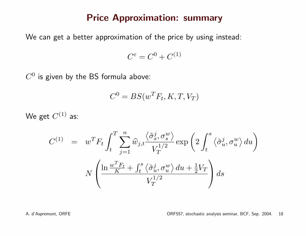
Price Approximation: summary

We can get a better approximation of the price by using instead:

Cε = C0 + C(1)

C0 is given by the BS formula above:

C0 = BS(wTFt, K, T, VT )

We get C(1) as:

C(1) = wTFt

∫ T

t

n∑

j=1

wj,t

⟨σj

s, σws

⟩

V1/2T

exp

(2

∫ s

t

⟨σj

u, σwu

⟩du

)

N

ln wT FtK +

∫ s

t

⟨σj

u, σwu

⟩du + 1

2VT

V1/2T

ds


Hedging Interpretation

• Suppose we are hedging the option with the approximate vol. σωs and, as

in El Karoui, Jeanblanc-Picque & Shreve (1998), we track the hedgingerror:

eT =1

2

∫ T

t

∥∥∥∥∥

n∑

i=1

ωi,sσis

∥∥∥∥∥

2

− ‖σωs ‖

2

(Fωs )

2 ∂2C0(Fωs , Vt,T )

∂x2ds

• At the first order in σjs, we get:

e(1)T =

∫ T

t

n∑

i=1

⟨σi

s, σωs

⟩ωi,sF

ωs

n(h(Vs,T , Fωs ))

V1/2s,T

ds

• We finally have:

C(1) = E[e(1)T

]


Outline

• Pricing baskets






Swaps

• The swap rate is the rate that equals the PV of a fixed and a floating leg:

swap(t, T0, Tn) =B(t, T floating

0 ) − B(t, T floatingn+1 )

level(t, T fixed0 , T fixed

n )

where


n ) =

n+1∑

i=1

coverage(T fixedi−1 , T fixed

i )B(t, T fixedi )


Swaps

• The swap rate can be expressed a basket of forward rates:

swap(t, T0, Tn) =

n∑

i=0

wi(t)K(t, Ti)

where K(t, Ti) are the forward rates with maturities Ti, with the weightswi(t) given by

wi(t) =coverage(T float

i , T floati+1 )B(t, T float

i+1 )


n )

• Empirically, these weights are very stable (see Rebonato (1998)).


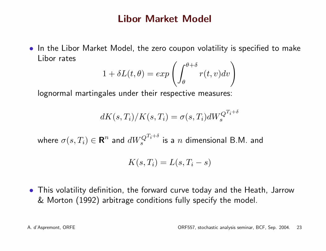
Libor Market Model

• In the Libor Market Model, the zero coupon volatility is specified to makeLibor rates

1 + δL(t, θ) = exp

(∫ θ+δ

θ

r(t, v)dv

)

lognormal martingales under their respective measures:

dK(s, Ti)/K(s, Ti) = σ(s, Ti)dWQTi+δ

s

where σ(s, Ti) ∈ Rn and dWQTi+δ

s is a n dimensional B.M. and

K(s, Ti) = L(s, Ti − s)

• This volatility definition, the forward curve today and the Heath, Jarrow& Morton (1992) arbitrage conditions fully specify the model.


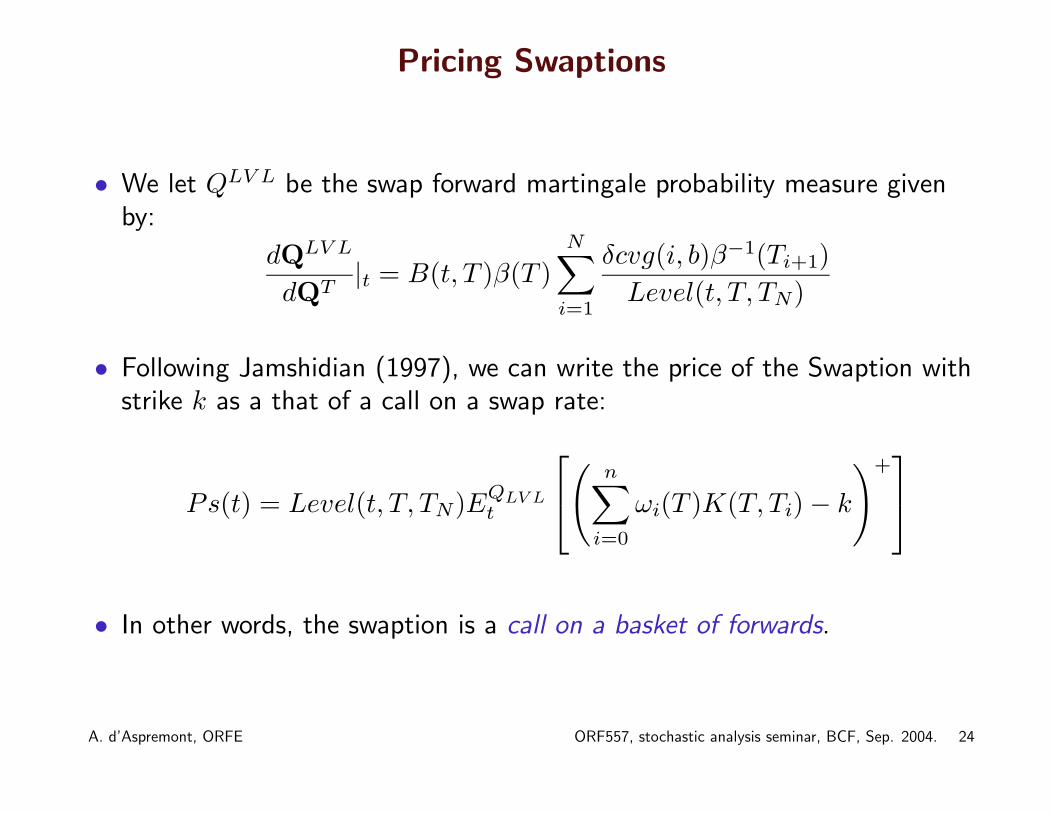
Pricing Swaptions

• We let QLV L be the swap forward martingale probability measure givenby:

dQLV L

dQT|t = B(t, T )β(T )

N∑

i=1

δcvg(i, b)β−1(Ti+1)

Level(t, T, TN)

• Following Jamshidian (1997), we can write the price of the Swaption withstrike k as a that of a call on a swap rate:

Ps(t) = Level(t, T, TN)EQLV Lt

(

n∑

i=0

ωi(T )K(T, Ti) − k

)+

• In other words, the swaption is a call on a basket of forwards.


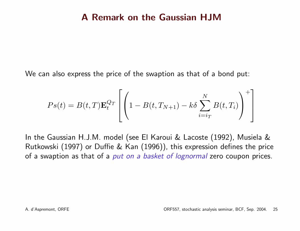
A Remark on the Gaussian HJM

We can also express the price of the swaption as that of a bond put:

Ps(t) = B(t, T )EQTt

1 − B(t, TN+1) − kδ

N∑

i=iT

B(t, Ti)

+

In the Gaussian H.J.M. model (see El Karoui & Lacoste (1992), Musiela &Rutkowski (1997) or Duffie & Kan (1996)), this expression defines the priceof a swaption as that of a put on a basket of lognormal zero coupon prices.


Approximations

We will make two key approximations:

• We replace the weights wi(s) by their value today wi(t).

• We approximate the swap rate∑n

i=0 wi(t)K(s, Ti) by a sum of QLV L

lognormal martingales F is with:

F it = K(t, Ti)

anddF i

s/F is = σ(s, Ti − s)dWLV L

s


Swaption pricing formula

We can write the order zero price approximation for Swaptions:

Swaption = Level(t, T, TN)(swap(t, T, TN)N(h) − κN(h − V

1/2T )

)

with

h =

(ln(

swap(t,T,TN)κ

)+ 1

2VT

)

V1/2T

where

VT =

∫ T

t

∥∥∥∥∥

N∑

i=1

ωi(t)σ(s, Ti − s)

∥∥∥∥∥

2

ds and ωi(t) = ωi(t)K(t, Ti)

swap(t, T, TN)

and dK(s, Ti) = σ(s, Ti − s)K(s, Ti)dWQTi+1s .


Errors

Can we quantify the error:

• What’s the contribution of the weights in the swap’s volatility?

• What about the drift terms coming from the forwards under QLV L?

• What is the precision of the basket price approximation?

First two questions: wait for next talk...


Price Approximation: Precision

We plot the difference between two distinct sets of swaption prices in theLibor Market Model.

• One is obtained by Monte-Carlo simulation using enough steps to makethe 95% confidence margin of error always less than 1bp.

• The second set of prices is computed using the order zero approximation.

The plots are based on the prices obtained by calibrating a BGM model toEURO Swaption prices on November 6 2000, using all cap volatilities and thefollowing swaptions: 2Y into 5Y, 5Y into 5Y, 5Y into 2Y, 10Y into 5Y, 7Yinto 5Y, 10Y into 2Y, 10Y into 7Y, 2Y into 2Y, 1Y into 9Y (choice based onliquidity).



Figure 2: Error (bp) for various ATM swaptions.



Figure 3: Error vs. moneyness, on the 5Y into 5Y



Figure 4: Error vs. moneyness on the 5Y into 10Y.



• We compare again with Monte-Carlo. The model parameters are

F i0 = 0.07, 0.05, 0.04, 0.04, 0.04

wi = 0.2, 0.2, 0.2, 0.2, 0.2

T = 5 years, the covariance matrix is:

11

100

0.64 0.59 0.32 0.12 0.060.59 1 0.67 0.28 0.130.32 0.67 0.64 0.29 0.140.12 0.28 0.29 0.36 0.110.06 0.13 0.14 0.11 0.16

• These values correspond to a 5Y into 5Y swaption.

• Our goal is to measure only the error coming from the pricing formula andnot from the change of measure/martingale approximation



0.2 0.4 0.6 0.8 1Moneyness in Delta

-0.0002

-0.0001

0

0.0001

0.0002Absolute

Error

Figure 5: Order zero (dashed) and order one absolutepricing error (plain), in basis points.



0 0.2 0.4 0.6 0.8 1Moneyness in Delta

-0.00005

0

0.00005

0.0001

0.00015

0.0002

0.00025

0.0003Absolute

Error

Figure 6: Order zero (dashed) and order one absolutepricing error (plain), in basis points, zero correlation.



0.2 0.4 0.6 0.8Moneyness in Delta

0

0.05

0.1

0.15

0.2

0.25Relative

Error

Figure 7: Order zero (dashed) and order one relativepricing error (plain), equity case.


Conclusion

• Order zero BS like formula sufficient for ATM swaptions

• Equity case: use order one

• Change of measure between QLV L and QT negligible (volatilities too low).

Next talk:

• Will discuss calibration and risk-management issues


Outline

• Pricing baskets






References

Black, F. & Scholes, M. (1973), ‘The pricing of options and corporateliabilities’, Journal of Political Economy 81, 637–659.

Carmona, R. & Durrleman, V. (2003), ‘Pricing and hedging spread options’,SIAM Rev. 45(4), 627–685.

Duffie, D. & Kan, R. (1996), ‘A yield factor model of interest rates’,Mathematical Finance 6(4).

El Karoui, N., Jeanblanc-Picque, M. & Shreve, S. E. (1998), ‘On therobustness of the black-scholes equation’, Mathematical Finance8, 93–126.

El Karoui, N. & Lacoste, V. (1992), ‘Multifactor analysis of the termstructure of interest rates’, Proceedings, AFFI .

Fournie, E., Lebuchoux, J. & Touzi, N. (1997), ‘Small noise expansion andimportance sampling’, Asymptotic Analysis 14, 361–376.


Heath, D., Jarrow, R. & Morton, A. (1992), ‘Bond pricing and the termstructure of interest rates: A new methodology’, Econometrica61(1), 77–105.

Jamshidian, F. (1997), ‘Libor and swap market models and measures’,Finance and Stochastics 1(4), 293–330.

Lebuchoux, J. & Musiela, M. (1999), ‘Market models and smile effects incaps and swaptions volatilities.’, Working paper, Paribas CapitalMarkets. .

Musiela, M. & Rutkowski, M. (1997), Martingale methods in financialmodelling, Vol. 36 of Applications of mathematics, Springer, Berlin.

Rebonato, R. (1998), Interest-Rate Options Models, Financial Engineering,Wiley.


Pricing basket options with an eye on swaptions

Documents

Transcript of Pricing basket options with an eye on swaptions