
Pricing at the On-ramp to the Internet: Price Indices for ...
69
Pricing at the On-ramp to the Internet: Price Indices for ISPs during the 1990s. Greg Stranger and Shane Greenstein* Abstract We estimate hedonic price indices for dial-up ISPs in the United States from November 1993 to January 1999. This was a period of rapid qualitative improvement in Internet access. We show that price indices without quality adjustment hardly changes after 1995, which we argue is a large error. Even with rather limited information, we estimate dramatic changes in prices from 1993 to 1996. We also estimate change in price per quality of 20% between late 1996 and early 1999. • This paper is partly derived from Stranger’s PhD dissertation at Northwestern University. We are, respectively, affiliated with the Boston Consulting Group and, Kellogg School of Management, Northwestern University. We thank Ernie Berndt, David Dranove, Barbara Fraumeni, Zvi Griliches, Brent Moulton, Scott Stern, and Jack Triplett for comments and suggestions. We received funding from the National Science Foundation, the Bureau of Economic Analysis and the Kellogg School of Management. All errors are our responsibility.
Transcript of Pricing at the On-ramp to the Internet: Price Indices for ...

Pricing at the On-ramp to the Internet: Price Indices for ISPs during the 1990s.
Greg Stranger and Shane Greenstein*
Abstract We estimate hedonic price indices for dial-up ISPs in the United States from November 1993 to January 1999. This was a period of rapid qualitative improvement in Internet access. We show that price indices without quality adjustment hardly changes after 1995, which we argue is a large error. Even with rather limited information, we estimate dramatic changes in prices from 1993 to 1996. We also estimate change in price per quality of 20% between late 1996 and early 1999.
• This paper is partly derived from Stranger’s PhD dissertation at Northwestern University. We are, respectively, affiliated with the Boston Consulting Group and, Kellogg School of Management, Northwestern University. We thank Ernie Berndt, David Dranove, Barbara Fraumeni, Zvi Griliches, Brent Moulton, Scott Stern, and Jack Triplett for comments and suggestions. We received funding from the National Science Foundation, the Bureau of Economic Analysis and the Kellogg School of Management. All errors are our responsibility.

Price indices for ISPs during the 1990s Greg Stranger & Shane Greenstein _____________________________________________________________________________________________
1
I. Introduction
Prior to commercialization the Internet was available for only researchers and educators.
Less than a decade after commercialization, more than half the households in the US were online
(NTIA, 2001). This growth presents many challenges for measuring the contribution of the Internet
to GDP. This study considers the formulation of consumer price indices for commercial Internet
access. We focus on constructing an index for the earliest period of growth of dial-up service, when
the challenges for index construction are greatest.
No simple measurement strategy will suffice for formulating price indices for Internet
activity. On average more than two thirds of time on line is spent at so-called free sites. Many of
these are simply browser-ware or Usenet clubs for which there is no explicit charge. Some of these
are partly or fully advertising supported sites. Households also divide time between activities that
generate revenue directly from use. For example, most electronic retailing does not charge for
browsing, but does charge per transaction. Other media sites, such as pornography, newspaper
archival and some music, charge directly for participation (Goldfarb, 2001).
There is one place, however, where almost every household transacts money for service.
Internet service providers (ISP’s) provide the point of connection for the vast majority of household
users, charging for such a connection. From the outset of commercialization most users moved away
from ISPs at not-for-profit institutions, such as higher education (Clement, 1998). Far more than
90% of household use was affiliated with commercial providers (NTIA, 2000). This continues today.
This paper investigates the pricing behavior at ISPs from 1993 to 1999 with the goal of
generating price indices. We begin with the earliest point when we could find data, 1993, when the

Price indices for ISPs during the 1990s Greg Stranger & Shane Greenstein _____________________________________________________________________________________________
2
commercial ISP market was still nascent. We stop in 1999 for a number of reasons. For one, the
industry takes a new turn with the AOL/Time Warner merger in early 2000, an event that we believe
alters strategies for accounting for qualitative change. Second, until the merger many industry
sources indicate that all on line provides follow the same technological trajectory. This helps us
construct indices without data on market share, which we lack. Until this merger we can test for (and
correct for) the most overt potential biases, as we show below. Third, and somewhat independently,
broadband began to diffuse just near the end of our sample. After a few years it did go to enough
households (7-8 million) to influence Internet price indices and alter the procedures done in this
paper. Finally, mid 2000 marks the end of unqualified optimism about the persistence of the Internet
boom. This change in mood was affiliated with restructuring of the ISP industry, potentially bringing
about a marked departure in price trends.
Using a new dataset about the early period, we compute a variety of price indices under
many different methods. The results show that ISP pricing has been falling rapidly over time. The
bulk of the price decline is in the early years of the sample, but a significant and steady decline
continues throughout. We test models that vary in their attention to aspects of qualitative change.
We find that this attention matters. Accounting for qualitative change shapes the estimates of price
declines and the recorded timing of those declines.
This paper is unique in that it is the first to investigate a large and long-term sample of U.S.
based ISP's. This setting gives rise to a combination of familiar and unique challenges for
measurement. This novelty and challenge should be understood in context. There have been many
papers on hedonic price indices in electronic goods (Berndt, Griliches, and Rappaport, 1995, Berndt,
Dulberger and Rappaport, 2000) and new industries, such as automobiles (Griliches, 1961, Raff and

Price indices for ISPs during the 1990s Greg Stranger & Shane Greenstein _____________________________________________________________________________________________
3
Trajtenberg, 1997). We borrow many lessons learned from those settings (See Berndt, 1991 for an
overview). There is also another paper about prices at Canadian ISPs (See Prud'homme and Yu,
1999), which has some similarities to our setting, though involving many fewer firms.
However, this is one of the first papers to investigate and apply these hedonic methods to
establish price indices for a service good. In this setting, physical attributes are not key features of
the service, but features of the contract for service are. These features can improve quite rapidly
from year to the next, as predominant contracting modes change, as new entrants experiment with
new service models for delivery, and as technical change alters the scope of possible services
available to ISPs. One of our primary goals is to understand hedonic price indices in such a market.
Many, but not all, ISPs offer more than one type of contract for service. In our data there is
no one-to-one association between firm and the features of service. This provides some challenges
for measurement, as well as some opportunities. We test different ways to control for unobserved
quality at the level of the ISP. We also assess the contribution to price changes from different
distinct strategies (at the firm level) of new entrants and incumbents. We find that new firms enter
the market at a small but significant price discounts to established incumbents. Related, when new
products/technologies are introduced, they are priced at a significant price premium to the existing
offerings. In contrast, we find that the ISPs who survive tend to have higher prices than younger
firms. Early in our sample, when new entrants gain market share, prices are driven down by entry.
Later in our sample, as incumbent firms manage to solidify their market shares in a growing market,
the pricing of incumbent firms takes on greater importance.

Price indices for ISPs during the 1990s Greg Stranger & Shane Greenstein _____________________________________________________________________________________________
4
II. A history of Internet Service Providers in the US
The Internet began as a defense department research project to develop networking
technologies more reliable than existing daisy-chained networks. The first product of this
research was ARPAnet. Later continuing research was supported by the National Science
Foundation, which established NSFnet, another experimental network for universities and their
research collaborators. NSF’s charter prohibited private users from using the infrastructure for
commercial purposes, which was not problematic until the network grew. By 1990 the TCP/IP
network had reached a scale that would shortly exceed NSF's needs and, possibly, managerial
reach. For these and related reasons, the NSF implemented a series of steps to privatize the
Internet. These steps began in 1992 and were completed by 1995. Diffusion to households also
began to accelerate around 1995, partly as a consequence of these steps and the
commercialization and diffusion of an unanticipated innovation, the browser (Greenstein, 1995).
II.1. The origins of Internet functionality and pricing.
A household uses commercial Internet provides for many services, most of which had
their origins in the ARPAnet or NSFnet. The most predominant means of communications is
email. The email equivalent of bulk mail is called a listserv, where messages are distributed to a
wide audience of subscribers. These listservs are a form of conferencing that is based around a
topic or theme. Usenet or newsgroups are the Internet equivalent of bulletin board discussion
groups or forums. Messages are posted for all to see and readers can respond or continue the
conversation with additional postings. Chat rooms and IRC serve as a forum for real-time chat.

Price indices for ISPs during the 1990s Greg Stranger & Shane Greenstein _____________________________________________________________________________________________
5
'Instant-messaging' has gained increased popularity, but the basic idea is quite old in computing
science: users can communicate directly and instantaneously with other users in private chat-like
sessions.
Some tools have been supplanted, but the most common are WWW browsers, gopher,
telnet, ftp, archie, and wais. Browsers and content have grown in sophistication from the one-line
CERN interface, through Lynx and Mosaic to the most up to date versions of Netscape Navigator
and Internet Explorer. The Internet and WWW are now used for news and entertainment,
commerce, messaging, research, application hosting, videoconferencing, etc. The availability of
rich content continues to grow, driving demand for greater bandwidth and broadband
connectivity.
L o c a lA c c e s s
P r o v i d e r s
R e g i o n a lA c c e s s
P r o v i d e r s
N a t i o n a lB a c k b o n eO p e r a t o r s
C u s t o m e r I PN e t w o r k s
S p r i n t , M C I , A G I S , U U n e t , P S I N e t
I S P 1 I S P 2 I S P 3
C o n s u m e r s a n d b u s i n e s s c u s t o m e r s
N A P N A P
Pricing by Internet Service Providers requires a physical connection. The architecture of
the Internet necessitates this physical connection. Both under the academic and commercial
network, as shown in Figure 1, the structure of the Internet is organized as a hierarchical tree.
Each layer of connectivity is dependent on a layer one level above it. The connection from a

Price indices for ISPs during the 1990s Greg Stranger & Shane Greenstein _____________________________________________________________________________________________
6
computer to the Internet reaches back through the ISP to the major backbone providers. The
lowest level of the Internet is the customer’s computer or network. These are connected to the
Internet through an ISP. An ISP will maintain their own sub-network, connecting their POP’s
and servers with IP networks. These local access providers get their connectivity to the wider
Internet from other providers further upstream, either regional or national ISP’s. Regional
networks connect directly to the national backbone providers. Private backbone providers
connect to public (government) backbones at network access points.
II.2. The emergence of pricing and services at commercial firms.
For this study, an ISP is a service firm that provides its subscriber customers with access
to the Internet. These are several types of “access providers.” At the outset of the industry, there
was differentiation between commercial ISP’s, “online service providers,” (“OSP’s” - Meeker
1996) and firms called “commercial online services” by Krol (1992). ISPs offer Internet access
to individual, business and corporate Internet users, offering a wide variety of services on top of
access, which will be discussed below. Most OSP’s evolved into ISPs around 1995-96, offering
the connectivity of ISP’s with a greater breadth of additional services and content.
Most households physically connect through dial-up service, although both cable and
broadband technologies gained popularity near the end of the millennium. Dial-up connections
are usually made with local toll calls or calls to a toll-free number (to avoid long-distance
charges). Corporations often make the physical connection through leased lines or other direct
connections. Smaller firms may connect using dial-up technology. These physical connections
are made through the networks and infrastructure of CLEC’s, RBOC’s, and other
communications firms. Large ISP’s may maintain their own network for some of the data traffic

Price indices for ISPs during the 1990s Greg Stranger & Shane Greenstein _____________________________________________________________________________________________
7
and routing; the largest firms often lease their equipment to other ISPs for use by their
customers. Smaller ISP’s generally are responsible for the call handling equipment (modems,
routers, access concentrators, etc.) and its own upstream connection to the Internet, but may lease
services in some locations for traveling customers.
Figure 1 – Typical PSInet point-of-presence (circa 1996)
Charging for access occurs at the point of access by phone. Internet service providers
generally maintain points of presence (or POPs) where banks of modems let users dial in with a
local phone call to reach a digital line to the Internet. Regional or national ISPs set up POPs in
many cities so customers don't have to make a long-distance call to reach the ISP offices in
another town. Commercial online services, such as America Online, have thousands of POPs
across many countries that they either run themselves or lease through a third party.

Price indices for ISPs during the 1990s Greg Stranger & Shane Greenstein _____________________________________________________________________________________________
8
Many ISPs provide services that compliment the physical connection. The most
important and necessary service is an address for the user's computer. All Internet packet traffic
has a 'from' and 'to' address that allows it to be routed to the right destination. An ISP assigns
each connecting user with an address from its own pool of available addresses. ISP’s offer other
services in addition to the network addresses. These may include e-mail servers, newsgroup
servers, portal content, online account management, customer service, technical support, Internet
training, file space and storage, web-site hosting, web development and design. Many larger
ISP’s also bundle Internet software with their subscriptions. This software is either private -
labeled or provided directly by third parties. Some of it is provided as standard part of the ISP
contract and some of it is not (Greenstein, 1999). Some ISP’s also recommend and sell customer
equipment they guarantee will be compatible with the ISP’s access equipment.
There are many different types of ISP’s. The national private bac kbone providers (i.e.
MCI, Sprint, etc) are the largest “ISP’s.” The remaining ISP’s range in size/scale from
wholesale regional firms down to the local ISP handling a small number of dial-in customers.
There are also many large national providers who geographically serve the entire country.
Many of these are familiar names such as Earthlink/Sprint, AT&T, IBM Global Network,
Mindspring, Netcom, PSINet, etc. The majority of providers provided limited geographic
coverage. A larger wholesale ISP serves all ISP’s further up the connectivity chain. Local ISP’s
get connectivity from regional ISP’s who connect to the national private backbone providers. A
large dialup provider may have a national presence with hundreds of POP’s, while a local ISP
may have only 1 POP and serve a very limited geographic market. Ultimately ISP’s are selling

Price indices for ISPs during the 1990s Greg Stranger & Shane Greenstein _____________________________________________________________________________________________
9
and servicing connectivity to the Internet. All computers that reach the Internet are connected
through some form of ISP.
It is difficult to describe modal pricing behavior for ISPs because there has been so much
change over time. The most likely date for the existence of the first commercial ISPs is 1991-92,
when the NSF began to allow commercialization of the Internet.1 In one of the earliest Internet
“handbooks,” Kro l (1992) lists 45 North American providers (8 have national presence). In the
second edition of the same book, Krol (1994) lists 86 North American providers (10 have
national presence). Marine (1993) lists 28 North American ISP’s and 6 foreign ISP’s. Sc hneider
(1996) lists 882 U.S ISP’s and 149 foreign ISP’s. Meeker (1996) reports that there are over 3000
ISP’s, and the Fall 1996 Boardwatch Magazine’s Directory of Internet Service Providers lists
2934 firms in North America. This growth was accompanied by vast heterogeneity in service,
access, and pricing. Descriptions of regional/wholesale connectivity (see Boardwatch
Magazine’s Directory of Internet Service Providers (1996)) imply that contracts are short-term.
II.3. Pricing behavior at commercial firms and how it changed.
Initially, the ISP pricing model mimicked what came before “Commercial Internet
access.” These services have similarities to Internet access, but they also differed from what
came next. Prior to the Internet, there were many bulletin boards and other private networks.
The bulletin boards were primarily text-based venues where users with similar interests
connected, exchanged email, downloaded/uploaded files and occasionally participated in ‘chat’
1 The earliest ISP’s were academic institutions that offered access to students and faculty over campus networks and through dial-in servers from off-campus. PSINet, a now bankrupt ISP, used to claim that it was the first commercial ISP, offering connection in 1991, though we have never found precise documentation for this claim

Price indices for ISPs during the 1990s Greg Stranger & Shane Greenstein _____________________________________________________________________________________________
10
rooms. The private networks or OSP’s (e.g. AOL, CompuServe, Genie, and Prodigy) had similar
functionality, with segregated content areas for different interests. Users could post and
download files, read and post interest group messages (similar to today’s Internet newsgroups,
but usually moderated). These forums (as they were called on CompuServe) were often centered
on a specific topic and served as a customer service venue for companies. The pricing structure
of the majority of these services was a subscription change (on a monthly or yearly basis) and
possibly an hourly fee for usage.
At this early stage, circa 1992-1993, most users would batch together the work they
needed to do online, connect, and quickly upload and download files, email, and messages. Then
they would disconnect, minimizing time online. Specialized software existed to facilitate this
process. When ISPs first commercialized in 1992, there were similar expectations that users
would continue to use the Internet in such bursts of time.
Because much of the usage was for uploading and downloading, it was sensible to charge
more for faster access. Pricing by speed when much of the online time is not idle is close to
pricing by volume (or pricing for traffic). Consequently, many ISPs services varied the hourly
charge based on the speed of the connection. In the early 1990’s speeds moved from 300 bps to
1200, 2400, 4800, 9600 and eventually to 14’400 and 28’800. The latter two were the norm of
the mid 1990s. 56K (or realistically, 43,000bps) became the norm in the latter part of the 1990s.
As speeds changed and as behavior changed, there were a variety of pricing plans. These
changed over time. Early on price plans began to offer larger amounts of hours that were
included in the monthly fee and offered marginal pricing above those included hours. These
plans offered traditional non-linear pricing or quantity discounts. In these plans, the marginal

Price indices for ISPs during the 1990s Greg Stranger & Shane Greenstein _____________________________________________________________________________________________
11
hours would be priced lower than the average cost of the included hours. We will say more
about this below.
Only later, after the ISP industry began to develop, and users demonstrated preferences
for a ‘browsing’ behavior, pricing began to shift to unlimited usage for a fixed monthly price.
These plans are commonly referred to as ‘flat-rate’ or ‘unlimited’ plans. These unlimi ted plans
caused capacity issues at POP’s because the marginal cost to the user was zero and some users
remained online much longer than the companies had expected. ISP’s reacted to this behavior by
introducing plans with high initial hourly limits and high marginal pricing above the limit. As
we document below, most such plans were not particularly binding unless the user remained on-
line for hours at a time most days of the month. In these plans the marginal cost of an extra hour
exceeded the average cost of the included hours. Some ISPs also instituted automatic session
termination when an on-line user remained inactive, eliminating problems arising from users
who forget to logoff.
In the later part of the 1990s the pricing of contracts depended less on speed because the
speed experienced by users was more dependent on customer modems than on POP equipment.
The menus of plans commonly include ‘unlimited’ use plans for $15 -$20 per month. Some
ISP’s also offer high limit fixed price plans with and withou t ‘penalties’ above the monthly limit.
The menu usually also includes a plan aimed at infrequent or low volume users. These plans
may cost $5-$10 and include 5-15 hours of online usage with marginal pricing above those
limits. Some menus include intermediate plans that fall somewhere between those above.
II.4. The structure of the ISP market also influenced pricing.

Price indices for ISPs during the 1990s Greg Stranger & Shane Greenstein _____________________________________________________________________________________________
12
The ISP market began to experience explosive entry around 1994-95, accelerating after
the commercialization of the browser around the same time (Greenstein, 2001). Early movers in
this market all had experience with the network used in higher education. Firms such as PSINet,
IBM, and MCI tried to stake positions as reliable providers for business and each achieved some
success over the next few years. When MCI and Uunet eventually became part of WorldCom in
1998 (subject to a restructuring and sell-off of some assets, as instituted by the Department of
Justice) WorldCom became the largest backbone providers in the US and one of the largest
resellers of national POPs to other firms. When IBM sold its facilities to AT&T in 1997, it
became one of the largest business providers of access in the US.
A signal event in 1995-96 was the entry of AT&T’s Worldnet service, which was
explicitly marketed at households. It became associated with reliable email and browsing, as
well as flat rate pricing at $20 a month, which imposed pricing pressure on other ISPs throughout
the country. This service eventually grew to over a million users within a year, though its market
growth eventually stalled. Indeed, it never met forecasts from 1995 that it would dominate the
market because, in effect, its competitors also grew rapidly. Growing demand for all services
meant that no player achieved dominance for several years.
The on-line service providers – Prodigy, Genie, CompuServe, MSN, and AOL – all
began converting to Internet service around 1995, with some providing service earlier than
others. All failed to gain much additional market share from this move except AOL, who used
this conversion as an opportunity to alter their service’s basic features. When AOL converted
fully to Internet access in 1996 it experienced quite a difficult transition because management
under-anticipated their own user’s response to the introduction of flat rate pricing. This bad

Price indices for ISPs during the 1990s Greg Stranger & Shane Greenstein _____________________________________________________________________________________________
13
publicity also facilitated further entry by other firms looking to pick up customers who fled the
busy phone lines. AOL survived the bad publicity through a series of new investments in
facilities and intense marketing. Furthermore, in 1997 it made a deal with Microsoft to use
Internet Explorer, which allowed it to grow at MSN’s expense, who had been one of its main
competitors until that point (Cusumano and Yoffie. 1999). In 1998 AOL bought CompuServe, a
merger that, in retrospect, initiated it on the path towards solidifying its leadership of dial-up
service.
Neither AT&T’s entry, nor IBM’s or MCI’s positioning, had satisfied all new demand.
Thousands of small entrepreneurial ventures also grew throughout the country and gained
enough market share to sustain themselves. New entrants, such as Erols, Earthlink, Mindspring,
Main One, Verio, and many others, gained large market positions. Some of these positions were
sustained and others were not. Private label ISPs also emerged when associations and affiliation
groups offered re-branded internet access to their members. These groups did not own or operate
an ISP, instead their access was being repackaged from the original ISP and re-branded by the
association. These firms could survive on relatively low market shares, though, to be sure, they
were not very profitable either.
By 1997 more than 92% of the US population had access to a competitive market filled
with a wide variety of options, with another 5% of the population – found in many different rural
locations throughout the US -- having access to at least one firm by a local phone call (Downes
and Greenstein, 2001). Economies of scale and barriers to entry were quite low, so thousands of
firms were able to sustain their businesses. Roughly speaking, market share was quite skewed. A
couple dozen of the largest firms accounted for 80% of market share and a couple hundred for

Price indices for ISPs during the 1990s Greg Stranger & Shane Greenstein _____________________________________________________________________________________________
14
95% of market share, but there was so much turnover and fluctuation that estimates more precise
than this were hard to develop.
Just prior to the AOL/Time Warner Merger in 1999-2000, the ISP market remained in
flux. Broadband connections (DSL or cable) began to become available in select places –
primarily urban areas, offering these home users a faster and possibly richer experience. The so-
called “free” -ISP model also emerged in late 1998 and grew rapidly in 1999, offering free
Internet access in exchange for advertisements placed on the users’ screen. These firms
eventually signed up several million households. The scope of service also continued to differ
between ISPs, with no emergence of a norm for what constituted minimal or maximal service.
Some ISPs offered simple service for low prices, while other ISPs offered many additional
services, charging for some and bundling others within standard contracts.
Stated succinctly, over a six year period there were many changes in the modal contract
form and user behavior. Changes in the delivery of services and changes in user expectations
resulted in numerous qualitative changes in the basic service experienced by all users. The
structure of the industry also fluctuated and no dominant providers emerged until the end of
millennium. Until then, all players were buffeted by many of the same competitive forces.
II.5. Turbulent times and price indices.
For reasons we explain in a moment, it is important for price index construction that
AOL’s dominance of the dial -up service was not a self-evident outcome until the end of the
Millennium. This arises as a specific implication of understanding challenges for price index
construction during turbulent times.

Price indices for ISPs during the 1990s Greg Stranger & Shane Greenstein _____________________________________________________________________________________________
15
In a market as turbulent as this one, we are quite skeptical of traditional price index
construction using only measured prices weighted by market share, unaltered for qualitative
change and competitive conditions. Lack of accounting for quality is very problematic for this
service. Also, price and market share provide deceptive indicators of the true state of the market.
First, large improvement in the quality of service occurred and went unmeasured. These
changes were widespread, and not unique to any particular firm or any particular product. They
happened too frequently to be measured. Every surviving firm, whether big or small, had to
experiment often with different modes for delivery and different features in the service.
Second, market share was frequently in flux and such changes were likely to fall below
the radar screen of any government price record. Experimentation enabled many new entrants to
succeed in growing market share well after commercialization began. Yet, data on market share
normally is collected by government agencies at a frequency of two or three years at most. This
only coarsely reflects the rapid addition of new users over time (whose adoption is induced by
improvements in quality). Large market also does not necessarily indicate the presence or
absence of market power over time or stability in market outcomes.
Another third and subtle error arises in markets with persistent skewed market share, as
in this case. Market-wide experimentation imposed competitive pressure on incumbent behavior,
even when these were very large firms. Behaving as if they were “paranoid”, t he most nimble
largest firms of this era, such as AOL and Earthlink, did not stand still. This paranoia appeared
justified since the least nimble firms, such as AT&T WorldNet, did not keep up and,
consequently, did not prosper (after a spectacular start in 1995-96). Incumbent ISPs were
compelled to make frequent releases of upgrades their software, to spend lavishly on marketing,

Price indices for ISPs during the 1990s Greg Stranger & Shane Greenstein _____________________________________________________________________________________________
16
to add new features constantly, and to keep prices low by not charging for extras – to prevent the
growing young firms from cutting into the incumbent’s leads . Yet, most of these competitive
outcomes, except nominal prices, were not measured. In short, while it is usually ok to ignore the
behavior of small fringe firms, that omission (or de-emphasis) could be an error if the large and
small acted as if they were close substitutes. The small firms provide useful information about
the unmeasured activities of the large.
In a traditional price index the pricing behavior of a few large firms receives the bulk of
attention. This is the appropriate procedure when quality does not change rapidly, when market
shares are stable over time, and when the measured behavior of large firms shapes the experience
of most users. In our case, however, we are certain that quality changed rapidly, that market
share bounced around quite a bit, and that the large firms acted as if they were afraid of losing
market share to the small. These observations will push us to examine the behavior of all firms in
this market and not just the top dozen.
III. Dataset Description
The dataset used in this paper is compiled chiefly from issues of Boardwatch Magazine’s
Directory of Internet Service Providers. The directory debuted in 1996 and continued to be
published through 1999. Since 1998 the same publisher has maintained a list of ISP’s at
http://www.thelist.com. Before the directory was published, Boardwatch Magazine published
lists of Internet service providers in its regular magazine. These issues date from November 1993
until July 1995. Another handful of observations in the dataset were collected from the
contemporaneous ‘how-to’ Internet books that are listed in the references below.

Price indices for ISPs during the 1990s Greg Stranger & Shane Greenstein _____________________________________________________________________________________________
17
The sample covers the time period from November 1993 until January 1999,
approximately a 6-year period. The sample is an unbalanced panel, tracking a total of 5948 firms
with a total of 19217 price plan observations.2 The dataset consists of demographic information
about the ISP (name, location, phone, and web address). In each year there are also a variety of
other characteristics of the ISP that are measured. These include additional service offerings
such as dedicated access, ISDN access, web hosting and the price for web hosting,
cable/broadband access, and wireless access. Other ISP characteristics include whether they are
a national provider, and if so, how many area codes they serve, upstream bandwidth, and total
number of ports. There is additional data from a survey/test done by Boardwatch and the results
give the percentage of calls completed and the average speed of actual connections for the
national providers in 1998.
Each ISP is associated with one or more price plans from a given time period. Each price
plan observation includes the connection speed, monthly fee, and whether the plan offers limited
or unlimited access. If access is limited then there is information on the hourly limit threshold
and the cost of additional hours. In a given year, there may be multiple price plan records for a
given firm because they offer a variety of plans at different connection speeds. The published
information generally gives pricing for 28.8 access as well as higher speed access.3
2This data does not represent all firms in the industry. It is also clear that the two or three price plans generally listed by Boardwatch for any given provider at one specific time do not necessarily represent all plans available from that ISP. Greenstein (2000) confirms that the Boardwatch data was incomplete in terms of the number of plans actually offered by an ISP. However, Boardwatch does state that the plans represent “the majority of users at an ISP or the most frequently chosen plans.” This offers some comfort that the sample represents a majority of the plans offered by ISP’s and chosen by consumers. 3 Boardwatch mildly changed its formats from one year to the next. Depending on the year this higher speed plan could be for 64k or 128k ISDN access or for 56k access. It should be noted that the price plans for these higher

Price indices for ISPs during the 1990s Greg Stranger & Shane Greenstein _____________________________________________________________________________________________
18
Table 1 below summarizes the number of observations in the panel. The data has been
left largely unchanged from its published form. Four observations from the first 2 years were
dropped due to the fact that they were extreme outliers. They certainly were unpopular, but
because we lack market share, they had an overwhelming and undue impact on the early price
index results. No other cleaning of the data has been done, apart from simple verification and
correction of data entry. As Table 1 shows, the latter part of the sample period produces the
greatest number of observations. This is one indication of how fast this industry was growing.4
Approximately 21% of the observed plans have a hourly limit, and the majority of those
are accompanied by a marginal price for usage over that limit. As time progresses, the universe
of firms/plans grows and the speeds offered continue to increase. At the start of the sample,
prices are only given for 14.4 k connections. By the end of the data, 28.8k and 56k have been
introduced, and there are price observations at 64k and 128k ISDN speeds as well as a small
number of observations of T1 connection prices. For limited plans, the hours included in the
plans continues to increase over time. The number of plans with limitations is decreasing over
time as a proportion of the sample. The pattern in the mean of monthly prices is not easy to
discern.
speeds included no information about hourly limitations or marginal prices. I have chosen to treat them as unlimited plans. The other choice would be to attribute the same hourly limitations as the slower plan from the same firm in the same year, but I have no basis for doing so. 4 Another measure of the rapid growth and evolution of this market is evidenced by the publishing pattern of ISP information in Boardwatch. In 1993-95, the list of ISP’s is relatively short and is included in the magazine, but by 1996 the market is growing rapidly and the listing are published in a separate directory that is updated quarterly. By 1998, changes in the market have slowed enough that the directory is only updated and published semi-annually. Finally, by 1999 the directory is only published and updated on an annual basis.

Price indices for ISPs during the 1990s Greg Stranger & Shane Greenstein _____________________________________________________________________________________________
19
Greenstein (2000) uses another source of data and examines contracting practices for
1998. In that data approximately 59% of firms quote only one price schedule, approximately
24% quote two price schedules and 17% quote 3 or more. Of the single price quotes,
approximately 26% are for limited prices.5 In this dataset, 71% of the observations are firms
quoting only one price, 26% quote two prices and the remainder quote three or more prices. This
is also highlighted in Table 1, where the average is 1.2 price plan observations per firm. The
difference between the data here and in Greenstein (2000) seems to be that we have more firms
who quote only one plan and fewer firms that quote more than two plans. 6 It appears that the
data from the Boardwatch directories does not include all plans offered by each provider,
particularly when an ISP offers 3 or more options. Boardwatch appears to track well ISPs who
offer two or fewer options. We conclude that the dataset represents a subset of the plans offered
by each provider because the publishing format limited the variety of plans that an ISP could list.
One of the weaknesses of this dataset is the lack of quantity measures of subscribers and
usage. Without usage data, there is no way to weight the price observations in the calculation of
an ideal price index. At the same time, as noted above, we would be quite skeptical of an
outcome using such weighting. Still, we would prefer to experiment with and without weighting,
if only to see the consequences, rather to have no ability to experiment.
We construct our index assuming that most firms were responsive to the same
technological trends. We are confident that qualitative change found at one firm spread to others
quickly. Another way to say this is this: It is as if we are assuming that the measured
5 Greenstein (2000) p.20.

Price indices for ISPs during the 1990s Greg Stranger & Shane Greenstein _____________________________________________________________________________________________
20
improvement at the small firms is informative about the unmeasured improvements at the large.
We partly test this assumption later in the paper when we examine the sensitivity of price
estimates to the age of the ISP, which proxies for the durability of incumbency and stable market
presence.
We do not think this assumption makes sense after 2000. After the consolidation of
AOL's leadership and its merger with Time Warner, AOL begins to follow its own path. This is
also increasingly true for MSN after the browser wars end (in 1998) and after the entry of the
free ISPs, such as NetZero, whose spectacular growth ceases after 2001. Moreover, the rate of
unmeasured improvement in features of dial-up service begins to decline after the dot-com crash
in spring of 2001 (though introduction of new features does not end after that, to be sure). As
noted, the lack of market share is more problematic for a stable dial-up market, which, arguably,
starts to emerge after 1998, and obviously emerges when adoption of the Internet slows at
households, as it does by 2001 (NTIA, 2001). Indeed, as we show below, prices begin to
become sensitive to incumbency by 1998-99, the last year of our sample, suggesting that our
judgment was correct. Thus, we did not collect data after early 1999.
IV. Elementary price indices
The most elementary price index has already been displayed in Table 2. The means of
the monthly prices trace a sharp upward path from 11/93-5/96 with an even sharper fall from
6 See footnote 2

Price indices for ISPs during the 1990s Greg Stranger & Shane Greenstein _____________________________________________________________________________________________
21
5/96-8/96, followed by small increases to 1/98 and another steep fall in 1/99. The medians also
decline over time, but the changes are discrete.
The fundamental problem with the data presented in Table 2 is that the observations in
each time period reflect very different service goods. Table 3 shows that homogenizing the
sample does reduce the variation in the calculated means and medians. The price index based on
the means now only rises from 11/93 to 1/95 and falls for the remainder of the sample period.
This rise is persistent throughout the price indices in the paper. It is discussed in more detail in a
later section below. The index based on the median falls early in the sample period and then
remains steady for the remainder. This is indicative of the growing homogeneity across firms
and plans in the later part of the sample.
IV.1. Matched models.
A procedure such as “matched models” compares products that exist in 2 adjacent
periods. This could be an improvement over aggregating all products for comparison, but it also
suffers because it ignores the introduction of new products (at least until they have existed for 2
periods). This method also ignores the disappearance of older or obsolete products because there
is no natural comparison to the product after its last year. If quality is increasing, then matched
models will overstate the period-to-period index number, biasing higher the measured price
change.
Index Formula

Price indices for ISPs during the 1990s Greg Stranger & Shane Greenstein _____________________________________________________________________________________________
22
Dutot DutotI ,
, 1
i ti
i ti
P
P −
∑∑
Mean ratio of the prices
Carli CarliI ,
, 1
i t
i i t
PP
N−
∑
Mean of the price ratios
Jevons JevonsI
1
,
, 1
Ni t
i i t
P
P −
∏ Geometric mean of price ratios
Using the matched observations, it is possible to compute the values of Dutot, Carli and
Jevons indices. Briefly, given a number of prices for matching services – designated by ,i tP 7, the
following formulas are used to calculate the indices. To construct the “matched model” indices,
we matched price plans from the sample where firmi, speedj at timet are matched with firmi,
speedj at timet+1
In
Table 4 we show the analysis for this ‘strict’ matching, where both firms and speeds must
match for a plan to be included in the calculation.8 The hypergrowth and turnover of the industry
in the first few years results in relatively few matches in the 1993-1996 period. In 1996, 510
plans9 from 5/96 are matched into the 8/96 part of the sample. From 1996 to 1997 a similarly
7 The i subscript designates the price plan and t subscript designates the time period. 8 Even the strict matching is ignoring any change in hours. We have ignored if a plan switched between limited and unlimited. 9 Of the 1283 total plans in 5/96, only 702 can possibly match a plan in 8/96 because the remain 581 plans are either 64k or 128k plans which are not reported for any firms in the 8/96 data.

Price indices for ISPs during the 1990s Greg Stranger & Shane Greenstein _____________________________________________________________________________________________
23
large proportion of plans match. Although the absolute number of matching plans remains high,
the proportion of plans that are matched decreases toward the end of the sample.
It has been noted that the Carli index generally overestimates the index level and this
seems to be confirmed in the results in Table 4. This is because a single large or extreme value
of
1
0
PP swamps small values of
1
0
PP when averaged. The simplest explanation is that this price
ratio is unbounded above – price increases can exceed 100%, but the ratio is bounded below –
price decreases can only be 100% - to zero. The Dutot index is nothing more than a comparison
of the mean prices of the matched products. Because it is a simple average, the Dutot index is
also susceptible to influence by large outlying data. The Jevons index is quite different. As a
geometric average, the Jevons index works very efficiently in a large sample to reduce the
impact of outlying observations.
The results shown in suggest that prices are declining throughout the sample period. The
notable exception is the Carli index, which shows price increases in nearly every period except
May-96, where the sample is very small. The average AAGR for Jevons and Dutot indices for
the entire period is –7.8%. In all cases, the Jevons and Dutot indices agree on direction of price
change, despite differing on the exact magnitude of the change.
IV.2. Determinants of Price
Before proceeding to examine hedonic regressions and the associated price indices, we
motivate the selection of the hedonic price model. The speed and duration of the plan are
important as are complimentary service offerings. Contract length and set-up costs may also be

Price indices for ISPs during the 1990s Greg Stranger & Shane Greenstein _____________________________________________________________________________________________
24
important, but they are not recorded in this data. Firm quality, experience and the competitive
environment are also potential determinants of price.
One of the key developments in ISP service offerings over the 1993-1999 time period is
the move from limited and metered plans to largely flat-rate unlimited usage plans. As noted
earlier, in 1993, when ISP’s begin to offer services to consumers, there was little need for
unlimited plans. In Table 5, we show the mean fixed monthly cost of Internet access in this
sample of ISP’s. In each year, the mean price for limited contracts is below the mean price for
unlimited contracts. These differences are all statistically significant at 1%. The table also
illustrates the shift away from limited plans over the 1993-1999 timeframe. At the outset, the
limited plans make up roughly 50% of the sample plans. By 1999, limited plans make up just
over 10% of the plans in the sample. In 1999, limited plans are on average $0.91 per month less
expensive than unlimited plans.
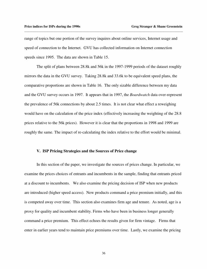
In Table 6, we continue to examine the effect of plan limitations on ISP pricing. The data
in the table show that for nearly every year, there is a persistent pattern to the mean prices and
the hourly limits. The lowest prices are from the contracts that include 10 hours or less in the
fixed price. As the hourly limits expand, so do the mean prices. This is true across all years
(except for 1/95) and the monotonic relationship is maintained until the limits exceed 100 hours.
Hour limitations above 100 hours seem to have no obvious relation to price that is consistent
across the observational periods in the sample.
Survey data from March 2000 show that 93.4% of users have monthly usage of 82 hours
or less and 90% of users have monthly usage of 65 hours or less. Thus it is not surprising that
limitations higher than 100 hours have little effect on ISP price. Comparing the higher limitation

Price indices for ISPs during the 1990s Greg Stranger & Shane Greenstein _____________________________________________________________________________________________
25
mean prices with the unlimited plans in Table 5, it is clear that these high limitation plans are not
priced very differently than the unlimited plans.
Other relevant variables are in Table 7. Connection speed is another important dimension
of Internet access. Over the full sample, there are observations from price plans that range from
14.4k at the low end up to some prices for T1 speeds (1.544 Mbs) at the upper end. As noted
earlier, these speeds should be given a broad interpretation. The changing nature of user
behavior influenced the marginal returns to faster connections.10
There are a number of other measures in the data set that could signal ISP quality. More
specialized types of access services being offered by an ISP could signal the technical expertise
of their staff and their reputation for quality and adoption of leading technology. While there are
many different ways to proxy for quality, we largely do not explicitly employ them in our
hedonic analysis.11 As we show below, however, we can use a random effects estimator which
correlates errors at an ISP over time. In part this will capture any unobserved quality that is
correlated at the same firm. We will also try to control for quality with vintage and age effects.
See more below. 12
IV.3. Hedonic Price Indices
10 Of course the other argument is that as connection speeds have improved, content providers have begun to offer richer content that uses higher transmission bandwidth. 11 We explored using such factors as whether the ISP provided national coverage, whether they provided additional services and some coarse measures of capacity, such as ports or T1 line backbone connections. These largely did not predict any better than well (or as well as the factors we left in the hedonic analysis). In addition, some of these were not available in all time periods, resulting in us using non-normalized measures of qualitative change over time. 12 For more on measuring quality at ISPs, see Augereau and Greenstein, 2001, Greenstein, 2000, or 2001.

Price indices for ISPs during the 1990s Greg Stranger & Shane Greenstein _____________________________________________________________________________________________
26
Hedonic models can be used to generate predicted prices for any product (i.e. bundle of
characteristics) at any given time. The first hedonic model that we will estimate is:
0 1 2 9 1 5ln ijt t ijt ijt ijt ijt ijt ijtP Year Limited dHrly Limited dSpeedα α β β γ ε− −= + + + ∗ + + (1.1)
Where the subscripts designate firm i, plan j, at time t. To divide the hourly limitations into
indicator variables, we examined the frequency plot of the hourly limits. We divided hourly
limits into different dummy variables. This will provide flexibility to coefficient estimates. Those
divisions and frequencies are shown in Table.
The specification in (1.1) was estimated for the whole pooled sample and for each pair of
adjacent time periods. Regression results are in Table 9. After testing the coefficients for each
of the hourly buckets, all but the lowest four were dropped from the model. The tests13 showed
that these coefficients were not significantly different from the coefficient on limited, because
they added no more information than the limited variable. In the unrestricted models (both
pooled and adjacent year models), the omitted hourly*limited indicator variable is for all hourly
limits above 250 hours. The omitted speed indicator variable is for plans offering 14.4k access.
The omitted time period indicator variable (year) is for 11/93.
The trend over time is that ISP’s offer increasingly fast connection speeds. Unlimited
plans have become more prevalent over time and the hours allowed under limited plans have
increased over time. These trends also indicate increases in “quality” over time. In the adjacent
13 For example testing H0: Hrs80*L – limited = 0

Price indices for ISPs during the 1990s Greg Stranger & Shane Greenstein _____________________________________________________________________________________________
27
period models, the time indicator variable is only being compared to the previous period. In the
pooled models, each coefficient on the time indicator variables represents a difference in price
relative to the omitted time period 11/93. In the pooled model, the coefficients should all be
negative and the coefficients of each succeeding period should be more negative than the
previous one, because the coefficient represents an accumulated price decline.
Limited plans should have a negative impact on prices, but that impact should be
decreasing as the number of hours allowed under the plan increases. For the regression, this
means that I expect the difference between the coefficients Hrs10*L and Limited to be negative.
Each difference should be smaller in absolute value as Limited is compared to higher-level
buckets, but the differences should remain negative (or approach zero – indicating that a high
limit plan is really no different than an unlimited plan).
Depending on which speed is omitted, the implication for the sign of the estimated
coefficients on the speed indicator variables varies. It does imply that higher speed plans should
have higher (more positive) coefficients than lower speed plans.
The regression results from model (1.1) appear in Table 9. The largest hourly limitation
buckets have been discarded from the full model, so I will focus on the coefficients of the
restricted model and the accompanying adjacent period regressions. In the restricted regression
(2nd column), all estimated coefficients are significant predominantly at the 1% or 5% level. The
coefficients on each of the speed variables confirm the hypothesis given above. The coefficients
for the higher speeds exceed the coefficients for the lower speeds and the pattern is
monotonically increasing. The differences between the hourly limitation variables coefficients
and the coefficient on limited also confirm the hypothesis given above. Plans with a limited

Price indices for ISPs during the 1990s Greg Stranger & Shane Greenstein _____________________________________________________________________________________________
28
number of hours are priced at a discount to unlimited plans and this discount diminishes as the
number of included hours increases.
The coefficients on the time indicator variables agree largely with the hypothesis given
above. Apart from the period from 11/93-1/95, the coefficients indicate that quality-adjusted
prices were falling, and the coefficients become more negative as the hypothesis described.
There are two interesting anomalies regarding the time indicator variable. The difference
between the coefficients on year95 and year96a is very large (indicating that 5/96 prices are
40% of the level of 1/95 prices). This dramatic large price decline needs to be investigated
further. The second interesting result from the regression is that prices appear to increase on a
quality-adjusted basis from 11/93-1/95. This is a recurring pattern through many of the models.
It is explained by the fact that the nature of Internet access changed during the intervening time
period. In 11/93 the connections that were offered were all UUCP (unix-to-unix copy)
connections that were capable of exchanging files, newsgroups and email, but had no interactive
features. By 1/95, all of the plans in the data are for SLIP (serial line internet protocol) access.
This is a more highly interactive connection that has all the capabilities of UUCP plus
other additional features (including multimedia capabilities).14 When the quality increase is the
same across all of the sample products, then it cannot be identified separately in a hedonic
regression from the time period indicator variable. Thus in 1/95 prices are higher than in 11/93,
but it is because Internet access technology has fundamentally changed. Because all the ISP’s
14 Looking carefully at the data and the advertisements, it’s clear that firms are promoting “slip” accounts as a premium service (as opposed to UUCP). The data seem to indicate that they are charging a premium for it as well. Because there is no heterogeneity among the 1/95 plan options, it is impossible to identitify this effect and separate it from the time period constant.

Price indices for ISPs during the 1990s Greg Stranger & Shane Greenstein _____________________________________________________________________________________________
29
have adopted the new type of access and “quality” has increased, there is no heterogeneity in the
sample and no way to control for the “quality” change. More to the point, this p roblem is
especially pronounced here; there is massive entry of new web services over time, but all the
ISPs provide similar access, so this entry is not identifiably different than the time dummy.
The right side of Table 9 displays the results from the adjacent period regressions. The
pooled model is a significant restriction on the data. In the pooled model, intercepts may vary
across time, but the slopes with regard to the characteristics are restricted to be equal across
periods.15 The adjacent period models relax this restriction so that the slopes are restricted to be
equal only across two periods in any model. Although some of the coefficients among the
adjacent period models are statistically insignificant, the majority confirm the hypotheses given
above. The hourly limitations and speeds affect price in the same way as the pooled model.16
The price increase in 1/95 is indiscernible because although the coefficient has a positive sign, it
is not significant. The remaining inter-period indicators are of negative sign and the steep
change in price from 1/96 to 5/96 is still present and very significant.
The coefficients from the hedonic regression model in (1.1) lead directly to a calculation
of the estimated price indices. These estimates are a consequence of the form of the model. By
exponentiating both sides of (1.1), it is clear that each parameter affects price in multiplicative
fashion. This aspect of the model, combined with indicator variables, simplifies the interpretation
15 I have not yet tested for parameter stability (i.e. tested to see if this restriction is valid). 16 The coefficients on the hourly limitations and speeds appear to be of the same magnitude across the differing time periods. While that suggests parameter stability over time and argues for the pooled model, I have not tested the restriction formally.

Price indices for ISPs during the 1990s Greg Stranger & Shane Greenstein _____________________________________________________________________________________________
30
of the regression coefficients. An adjacent year model17 is the simplest case. The column
marked 93/95 in Table 9 displays the results for an adjacent period regression pooling only the
data from the 11/93 and 1/95 time periods. The first variable listed after the constant term is
Year95 which is an indicator variable for all plans that are from the 1/95 time period. The
estimated coefficient on the variable Year95 is 0.058 (from Table 9). The direct method to
calculate a price index uses this estimated coefficient. For this model, the hedonic price index
would be 0.058 1.0597e = at the time period 1/95 (relative to a base value of 1.00 at the 11/93) time
period.
By using this method, the models estimated in Table 9 lead directly to estimated price
indices. These are shown in Table 1. By exponentiating the estimated coefficients of the yearly
dummies, I can calculate the price indices directly. In the model covering, the whole sample
period, the calculated index will be cumulative (i.e. year base
)exp(Index
Indextt =α ). These are easily
reconverted to period-to-period indices. The models in Table 9 that consider adjacent time
periods also lead directly to estimates of the period-to-period indices. These are calculated in the
same manner.
The results of these calculations are shown in Table 1. The table shows that the
cumulative “quality adjusted” index declines 58% to 0.422 in 1/99 when compared to 1.00 in the
base period, 11/93. The individual period-to-period indices display large variation during the
17 Refer to Table 9.

Price indices for ISPs during the 1990s Greg Stranger & Shane Greenstein _____________________________________________________________________________________________
31
initial periods, but then moderate to a 1-10% decline per period.18 The calculations from the
adjacent year regressions are largely the same as the results from the restricted model. The
exception is the 11/93 to 1/95 index which displays a less extreme rise during the time period
under the adjacent years method. The extreme drop in the index from 1/95 to 5/96 is still present
and remains an open question to be further explored.
IV.4. Hedonic Price Indices with random effects
The dataset covers very few characteristics of each plan/product, and there are
undoubtedly unmeasured elements of quality that are missing from model (1.1). Because of the
(unbalanced) panel nature of the dataset, the firm-specific unmeasured quality can be corrected
using a random-effects model.19 In this case the regression model given above in (1.1) will be
changed by adding a firm specific error term ( iυ ).
0 1 2 9 1 5ln ijt t ijt ijt ijt ijt ijt i ijtP Year Limited dHrly Limited dSpeedα α β β γ υ ε− −= + + + ∗ + + + (1.2)
We have estimated both the fixed and random effects specifications of model (1.2). The
regression results are shown in Table 2. The Breusche-Pagan test indicates that the hypothesis
that var( iυ ) = 0 can be rejected with better than 1% certainty. The Hausman specification test
also indicates that the random effects specification is preferred to the fixed effects model.
The random effects regression results differ from the earlier results. The main difference is that
the drop in prices ascribed to 1/95 to 5/96 period is dampened. The pattern among the time
18 It is difficult to compare all of the adjacent period indices. Each time period is of different length, so for accurate and easier comparison, it would be correct to annualize the changes.

Price indices for ISPs during the 1990s Greg Stranger & Shane Greenstein _____________________________________________________________________________________________
32
period indicator variables is maintained. The significance and pattern among the plan limitations
fits with earlier hypotheses and follows the pattern of the earlier results. The coefficients on the
speed indicator variables also follow the pattern outlined in the hypotheses above and reconfirm
the results from the earlier regression. Table 2 also shows the adjacent period regression results.
They also follow the pattern of the earlier results with again the main difference being a
dampened drop in the index from 1/95 to 5/96.
Using the regression results from the random effects “restricted” model and the random
effects adjacent period model, we have recalculated the cumulative and period-to-period indices
in Table 3. The cumulative index drops from 1.00 in 11/93 to 0.51 in 1/99. This shows that
“quality” adjusted prices fell by 49% over this period. As before, the period to period indices
swing wildly in the initial periods, but then settle to steady declines of 0-7% per period. The
striking difference between the random effects model results and the earlier results is shown in
the period-to-period index from 1/95 to 5/96. Without random effects the index declined to 0.38
over this single period. Taking other unmeasured elements of firm quality into account dampens
this drop in the price index. In Table 3, the index only drops to 0.44. The index values
calculated from the adjacent period models are all nearly the same as the single period indices
derived from the pooled model. The only inconsistency is the 11/93 to 1/95 index, but this is an
insignificant coefficient in the adjacent period regression.
19 Of course the ‘omitted variable bias’ question arises here. Unless the omitted variable is correlated with one of the year dummies, then the direct index parameter estimates will be unaffected. I have not been able to find an example of a omitted characteristic of a dial-up plan that is correlated with time (or with any of the other variables).

Price indices for ISPs during the 1990s Greg Stranger & Shane Greenstein _____________________________________________________________________________________________
33
Firm level random effects alters the index. With so much entry and exit in the sample, it
is unclear from the above results what aspect of changing quality is unmeasured. We conclude
that accounting for measured and unmeasured quality is a simple and useful addition to the tools
for calculating price indices. It is a further refinement of the standard hedonic techniques, but it
is not difficult to implement. The results and statistical significances are easily interpreted.
IV.4. Analysis of sub-sample with speeds below 28.8
We were concerned that the results could be an artifact of change in modem speeds,
which is coincident with the transition to unlimited plans. We tested this by examining contracts
only for 28.8 service.
We have repeated the random effects modeling (model (1.2)) with a sub-sample of plans
that offer connection speeds at or below 28.8k.20 Table 4 shows the regression results from this
sub-sample. The results shown for the sub-sample correspond well to the full sample regression.
The coefficients display the same pattern as the earlier full-sample regressions, supporting the
hypotheses given above. Quality adjusted prices decline over the sample period, with the
coefficient for each time period being more negative than the last. The apparent quality adjusted
price rise from 11/93 to 1/95 persists, showing that this pattern is not an artifact of the higher
speed plans. The plans with hourly limitations reconfirm the pattern of the full sample.
Additional “limited” hours a re consistently more valuable, with the highest limited plans
nearly indistinguishable from “unlimited” plans. In the pooled regression, speed of a plan is
20 Although 56k connections are available during this period, the data in Table 15 suggests that dialup connections were dominated by lower speed until the spring of 1998.

Price indices for ISPs during the 1990s Greg Stranger & Shane Greenstein _____________________________________________________________________________________________
34
handled using a dichotomous variable indicating whether a plan is 14.4k or 28.8k. In the
regression, 28.8k plan indicator was the omitted category. The only result in this sub-sample that
conflicts with the earlier results is the coefficient on 14.4k speed plans. Recall the earlier
argument presented above that put forward the hypothesis that “faster ” plans should command a
price premium. To be consistent with that hypothesis, the coefficient on Speed14 should be
negative (because Speed28 is the omitted dichotomous variable). In Table 4, this coefficient is
positive and statistically significant.21
The adjacent period regressions are also shown in Table 4. Similar to the pooled model,
these regressions on the sub-sample largely reconfirm the results from the full sample. Prices
decline over time and larger limits are more valuable. In the 95/96a regression results, a similar
positive and significant coefficient appears for Speed14. This again is unexpected and runs
contrary to the hypothesis given above. The remaining adjacent period regressions do not control
for speed of plan because only 28.8k speed plans are considered in the remaining part of the
subsample.
Using the regression results from the random effects restricted model and the random
effects adjacent period model, we have recalculated the cumulative and period-to-period indices
in Table 14. The results are consistent with the results from the full sample. The cumulative
index show that prices in this sub-sample drop from 1.00 in 11/93 to 0.48 in 1/99. This shows
that “quality adjusted” prices have dropped by 52% over the sample period. This index in
consistent with the full sample cumulative index which dropped by 49% over the same period.
21 I do not currently have a “good” possible explanation for this apparently contradictory result. There may be an

Price indices for ISPs during the 1990s Greg Stranger & Shane Greenstein _____________________________________________________________________________________________
35
The single period calculations are consistent with the full sample results. Price increases between
the first two periods, followed by a sharp decline, and then steady declines of 1-7% thereafter.
Repeating the analysis of model (1.2) on a sub-sample of plans with speeds at or below
28.8k gives results that are very consistent with the analysis of the full sample. This suggests
that the treatment of the hourly limitations in the higher speed plans is not significantly skewing
the results for the full sample. It also suggests that although many new entrants appeared over
time offering higher speed plans, the pattern of “quality adjusted” prices was not different
between the “old” and “new” pro viders.22 The most important conclusion is that the unobserved
limits for the high speed plans are not affecting the overall results.
IV.5. Weighted Hedonic Price Indices
To calculate an ‘ideal’ price index, data is needed on the market shares or revenue s hares
of the product or service. The Boardwatch ISP pricing data did not contain such information.
Because the listings are organized by area codes served, we could use the number of area codes
served by each ISP as a coarse market share weighting. It would be a coarse measure because of
population density is not uniform across area codes and intra-area code market shares are not
evenly split. Another simpler alternative is to weight the plans based on the connection speed
offered. Such data is available from the GVU lab www surveys.
The Graphics, Visualization and Usability lab at the Georgia Institute of Technology has
conducted a WWW users survey semi-annually since January 1994. The surveys cover a broad
interaction of variables which is leading to this result, but I have yet to identify the problem. 22 The best test of this would be interaction terms for the time period x speed. This would explicitly allow investigation of the price paths within speed segments.
Price indices for ISPs during the 1990s Greg Stranger & Shane Greenstein _____________________________________________________________________________________________
36
range of topics but one portion of the survey inquires about online services, Internet usage and
speed of connection to the Internet. GVU has collected information on Internet connection
speeds since 1995. The data are shown in Table 15.
The split of plans between 28.8k and 56k in the 1997-1999 periods of the dataset roughly
mirrors the data in the GVU survey. Taking 28.8k and 33.6k to be equivalent speed plans, the
comparative proportions are shown in Table 16. The only sizable difference between my data
and the GVU survey occurs in 1997. It appears that in 1997, the Boardwatch data over-represent
the prevalence of 56k connections by about 2.5 times. It is not clear what effect a reweighing
would have on the calculation of the price index (effectively increasing the weighting of the 28.8
prices relative to the 56k prices). However it is clear that the proportions in 1998 and 1999 are
roughly the same. The impact of re-calculating the index relative to the effort would be minimal.
V. ISP Pricing Strategies and the Sources of Price change
In this section of the paper, we investigate the sources of prices change. In particular, we
examine the prices choices of entrants and incumbents in the sample, finding that entrants priced
at a discount to incumbents. We also examine the pricing decision of ISP when new products
are introduced (higher speed access). New products command a price premium initially, and this
is competed away over time. This section also examines firm age and tenure. As noted, age is a
proxy for quality and incumbent stability. Firms who have been in business longer generally
command a price premium. This effect echoes the results given for firm vintage. Firms that
enter in earlier years tend to maintain price premiums over time. Lastly, we examine the pricing

Price indices for ISPs during the 1990s Greg Stranger & Shane Greenstein _____________________________________________________________________________________________
37
decisions of firms that exit the sample. Firms who leave the sample offer higher prices in the
period before they leave.
V.1. Entrants
Numerous firms enter the dataset during each period. An open question is what were
entrants’ pricing strategies as they came into this market. Did entrants differentiate their service
in some meaningful dimension so that they could price at or above incumbents’ prices? Using
the hedonic regression techniques described above, it can be determined that the entrants do
price at a discount to incumbents and that there are no vintage effects.
This new model incorporates random effects and two new sets of regressors.
0 1 2 9 1 5ln ijt t ijt ijt ijt ijt ijt
t year t year i ijt
P Year Limited dHrly Limited dSpeed
Entrant Newfirm Vintage
α α β β γδ δ φ υ ε
− −= + + + ∗ + +
+ + + + (1.3)
The new regressors are entrant, newfirm(year), and vintage(year). In Table 17, the number
of price plans by entrants and incumbents is shown. The regressor entrant is a dichotomous
variable that denotes a firm that has entered the dataset for the first time. The regressor
newfirm(year) is also a dichotomous variable that more closely identifies new firms specific to
given years. This is the same idea presented above when limited plans were considered. Firms
are either an entrant or an incumbent, and if they are entrants they enter at a particular time
period. In Table 18, the number of price plans is shown for each vintage in the dataset. The
regressors vintage(year) allow tracking of firms that enter and remain in the sample. For instance,
the regressor Vintage97 is a dichotomous variable that marks every price plan for firms that

Price indices for ISPs during the 1990s Greg Stranger & Shane Greenstein _____________________________________________________________________________________________
38
entered the dataset in March-97. This vintage is marked for all further price plans from these
firms as they remain in the sample.
Table 19 displays the regression results about entrants, incumbents and firm vintage. The
regression results demonstrate that new entrants offer discounted pricing as they entered the
market. This is effect is largest and most significant in 1996 and 1999. The regression results
also demonstrate that new entrants not only offered discounted pricing upon entry, but tended to
continue discounted pricing over time.
The first regression shown in the left column of Table 19, is a restricted version of model,
including only the dichotomous variable entrant. In this regression, the coefficient on the
entrant variable is negative and significant at the 1% level. This indicates that entrants offered
roughly a 1.7% price discount when compared to their incumbent peers.
The regression shown in the second column of Table 19 is another less restricted version
of model (1.3), encompassing a variable for entry (entrant) and a set of interaction variables
indicating when an entrant entered (e.g. new*96a, new*96b). These entry dates coincide with
the first appearance of the firm and its service plans in the dataset. Similar to the variables that
cover limited plans, the sum of the coefficients on entrant and new*96a are the estimate for the
discounts offered by entrants at each particular observation period. It is the sum of these
coefficients that is tested for significance. The sum of the entry coefficients is negative for each
of the periods in the dataset. However, only the coefficients for firms that entered in May 1996
and January 1999 are significant at 1%.
The regression in the third column of Table 19 is another version of model (1.3). This
model includes dichotomous variables that mark the vintage of the firm and its price plans (e.g.

Price indices for ISPs during the 1990s Greg Stranger & Shane Greenstein _____________________________________________________________________________________________
39
vintage95 ̧vintage99). The coefficients on these vintage variables are relative to the omitted
vintage, 1993. The coefficients for each vintage are negative and significant in all cases except
1995. There is also a pattern among the coefficients. The coefficient on each subsequent vintage
is generally more negative than the coefficient on the preceding vintage. This indicates that
entrants priced lower on entry and that firms of the same vintage continued to keep prices lower
than firms that had entered at previous times. Tests of the differences show that all are
significant at various levels except the difference from 1997 to 1998, which does not indicate a
price decline.
The regression in the rightmost column of Table 19 is the unrestricted version of model
(1.3). This model incorporates all of the entrant variables as well as all of the vintage variables.23
The results of this model re-affirm the restricted models described above. The summed
coefficients on the new entrant variables are all negative except for 1997. The only sums that
show statistical significance are again May 1996 and January 1999 at the 1% level. The
coefficients on the vintage variables follow the same pattern of increasing discounted prices with
each set of new entrants. The significance of the differences between vintages is weaker than in
the unrestricted model in the third column because two of the four differences are statistically
significant. Those differences are between vintages 96a and 96b and vintages 97 and 98.
In each of the regression results shown in Table 19, the coefficients on time, limited
plans, and speeds are consistent with the earlier results. The coefficients on the observation
period (time) are also consistent in magnitude in the first regression shown in the left column of
23 vintage99 is omitted from the unrestricted model because it is the same as the interaction variable new*99.

Price indices for ISPs during the 1990s Greg Stranger & Shane Greenstein _____________________________________________________________________________________________
40
the table. These coefficients are less consistent in magnitude across the other restricted
regressions in Table 19, because the time coefficient is also partly accounted for in the
coefficient on the entrant*year variables. To a lesser degree this is also true of the vintage
variables.
These results on entrants support the hypothesis that competition between ISP’s was
partly fought through pricing. The regressions support the general notion that entrants came into
the market at a discount to the incumbents. This discount only amounts to perhaps $0.25 /month
on average, but it is a significant and persistent. Looking more carefully at individual points in
time, the results show that entrants in May 1996 and January 1999 were more aggressive and
offered prices significantly below the incumbents. These effects are re-affirmed when
examining the vintage effects. Subsequent classes of entrants offer lower and lower prices. It
also appears that these differences in price among entrants of varying years are persistent over
time.24
Altogether, the results support the view that entrants used price as a competitive weapon
to gain entry to this market. However, the estimated size of the discounts is not as large as might
be imagined. The results may also support the idea that subsequent entrants ‘learned’ this
behavior as the ‘accepted’ mode of competition in this market and priced lower on entry as a
consequence. These results also suggest that under-sampling successful new entrants would lead
to an upward bias in a price index.
24 This ‘vintage’ effect may be actually be masquerading as a combination of firm age and survivorship bias. If older, surviving firms signal quality and a loyal customer base, they would have higher prices. See the analysis of firm age in the section below.

Price indices for ISPs during the 1990s Greg Stranger & Shane Greenstein _____________________________________________________________________________________________
41
V.2. New Product/Technology
When new technology is introduced among ISPs, there are capital investments and
technological hurdles. The size of these hurdles and the demand for the new technology
determines the rate of adoption. The introduction of higher speed access by ISP’s involved the
adoption of new modem technology for both the ISP and the customer. When new modem
technologies have been introduced in the past, adoption has been gradual.25 This leaves the early
adopters with temporarily increased market power. It is an open question whether exploiting that
market power is in the long run best interest of the ISP, but in the short run, there is room to
price the new, higher speed service at a premium.
The effect of new products can be tested within the hedonic regression framework. To
understand the effect of new product introductions, we estimate the following model
0 1 2 9 1 5ln
56ijt t ijt ijt ijt ijt ijt
i ijt
P Year Limited dHrly Limited dSpeed
Entrant New NewBoth
α α β β γδ λ φ υ ε
− −= + + + ∗ + +
+ + + + (1.4)
Model (1.4) shows two dichotomous variables. new56 indicates 56k plans that are
introduced in March 1997. newboth indicates 28.8 speed plans when they are introduced into
the sample in January 1995 and 56k plans introduced in 1997. The model cannot use a
dichotomous variable to represent the introduction of 28.8 speed plans alone because it would be
equivalent to the linear combination of the Speed28 and Year95 variables. Rolling the new
products into one dichotomous variable imposes a restriction that the coefficient on each new
product variable (new28 and new56) is the same.
25 See Augereau (1999) for an account of the battle over the 56k modem standard and the effects on adoption.

Price indices for ISPs during the 1990s Greg Stranger & Shane Greenstein _____________________________________________________________________________________________
42
In January 1995, the first plans to offer 28.8 kbps dial-up access appear in the data. 11%
of the plans in the dataset (5/47) in 1995 were the first 28.8 plans to appear. The remainder of
the plans in the 1995 data is 14.4 kbps plans. When 56 kbps plans first appear in the data in
March 1997, they represent 12% of the plans in that portion of the data (446/3813). The
remaining plans in the 1997 data are 28.8 kbps speed plans.
Table 2020 displays the regression results for full and restricted versions of model (1.4).
As mentioned above, there are no results with a distinct estimation of the coefficient on new28.
In the model in the left column (‘NewProducts’), a restricted version of the (1.4) model is
estimated using the combined newproduct variable newboth. The results show that the
estimated coefficient on the newboth variable is positive and significant at better than the 1%
level. In the model in the center column, the regression estimates the effect of the introduction
of 56k plans that first appear in the dataset in March 1997. The results show that the estimated
coefficient on the new56 variable is positive and significant at better than the 1% level. The
results shown in the right column are for the unrestricted version of model (1.4). This version of
the model incorporates the combined new product variable newboth and the newfirm variable
used in the entrant/incumbent analysis above. These results show that the estimated coefficient
on the newboth variable is positive and significant at better than the 1% level. The estimated
coefficient on the newfirm variable is positive and significant at the 1% level and also consistent
in magnitude with the results from the earlier section.
In each of the results in Table 2021, the estimated coefficient on the new product
variables is approximately the same magnitude. The estimated coefficients imply that new
products were introduced at approximately a 24% price premium. This is consistent with the

Price indices for ISPs during the 1990s Greg Stranger & Shane Greenstein _____________________________________________________________________________________________
43
hypothesis given above that ISPs would exploit temporary market power when they introduced
new higher speed plans.
The other results in Table 20 and 21 are mostly consistent with the results in earlier
sections. The coefficients on the variables for limited plans and the speed of connections are all
consistent with the earlier results. The coefficients on each of the time variables do vary
significantly in the regressions that contain the newboth variable. The coefficients on the time
variables in the center column indicate a pattern for the price index that is consistent with earlier
results.
However, the results shown in the left and right columns of the table are much different
than the earlier results. The main difference is in the coefficient on the variable Year96a. The
estimated coefficient for this variable is higher (less negative) than in the earlier hedonic price
index results. This is important because the coefficient represents a cumulative decline since the
11/93 start of the dataset. One possible explanation of this different result is that the price
premium given to the 28.8 speed plans in 1/95 was fleeting and if unaccounted for, the price
index would appear to fall even more quickly from 1/95 to 5/96. If the new 28.8 plans in 1/95
are isolated and given a fixed price premium of 22%, then when they are not “new products” in
the next time period, the price does not seem to have fallen as much over that time period. This
is because much of the price drop can be attributed to scarcity of 28.8 speed plans and the market
power and premium pricing that was attached to them in 1/95. In the subsequent time periods,
inter-period declines in quality-adjusted prices are consistent with the results given in the earlier
hedonic regressions above. This implies that instead of dropping 49% overall price index only
declines to 0.615 or a drop of 38.5%. Moreover, the pattern of price declines is largely the same

Price indices for ISPs during the 1990s Greg Stranger & Shane Greenstein _____________________________________________________________________________________________
44
except from 1/95 to 5/96, where the price index declines much less rapidly than before, dropping
from 1.33 to 0.73.
When ISP’s first had the capability to offer new higher speed plans, some did. The
results show that they exploited their temporary market power and charged an estimated
premium of 24% above the expected quality adjusted price.
V.3. Firm age/tenure
Following the example of Berndt et al, 1994, we next calculated hedonic estimates with a
full array of age and vintage effects. The length of time a firm is in the sample may signal a
number of effects. It is unclear from looking at the simple averages that there is an easy answer.
There are reasonable arguments to expect that increased tenure in the sample would have a
positive effect on pricing, namely as a signal of quality and as a signal of management
competence. There could also be lock-in and loyalty effects that would sustain higher prices for
older firms. But there are also reasonable arguments that would suggest a negative effect such as
a lower cost position gained through accumulated learning.
In this context age is the number of times a firm has shown up in the data with at least
one price plan. At the beginning of the sample, the industry has just started and all firms are of
the same age. As the industry grows and matures from 1993-1999, many firms enter, some firms
exit and some firms consolidate. By the end of the observational period there is quite a
dispersion of the age of firms. There are several firms that have been in the sample at every
period and others who are new in 1/99. The majority fall somewhere in between.
There are many possible effects here. One effect concerns survivorship bias and is akin
to the quality signals that were discussed above in the section concerning the provision of

Price indices for ISPs during the 1990s Greg Stranger & Shane Greenstein _____________________________________________________________________________________________
45
technically complex services. Firms that have survived the growth and transitions in this
industry must be successfully providing value to their customers. This quality effect would
argue that “older” ISP’s can charge premium prices because they offer higher quality.
The second effect concerns loyal customers, lock-in and switching costs. For some types
of customers, the technical challenge of getting service from another ISP may raise some
switching costs. Network effects from content and communications platforms that are
proprietary to the ISP may help with customer lock-in. If older ISP’s are more likely to have
loyal customers with some degree of switching costs and lock-in, then these ‘older’ ISP’s to be
able to charge a price premium versus their less experienced, less established competitors.
A third possible effect is that older firms have ‘produced’ more Internet service in the
time they have been in business. If there are learning curve effects, such as the optimal
customer/port/bandwidth ratios, then older firms may have a knowledge and cost advantage over
younger firms. This effect would argue for lower prices from older firms due to potential cost
advantages.
We have created a variable age that counts the number of months that a firm is observed
in the sample. The minimum age of any firm is 0 if they are a new entrant. The next shortest
would be 3 months if they enter in 5/96, reappear in 8/96 and subsequently disappear. The
longest life for a firm would be 62 months if it entered the sample in 11/93 and continued to
appear through the last data point at 1/99. At each time point in the data, the age of the firm is
recalculated back to its entry and this age is attached to the price plans from that set of

Price indices for ISPs during the 1990s Greg Stranger & Shane Greenstein _____________________________________________________________________________________________
46
observations.26 To determine the effects of firm age, the hedonic regression framework is again
employed to estimate the following model.
0 1 2 9 1 5ln ijt t ijt ijt ijt ijt ijt i ijtP Year Limited dHrly Limited dSpeed FirmAge NewBothα α β β γ δ φ υ ε− −= + + + ∗ + + + + + (1.5)
Table 21 shows the regression results. The two models shown are the hedonic random-
effects model (1.2) and the estimation of model (1.5) with the variables firmage and newboth
from the previous section. The results show that the estimated coefficient on the variable
firmage is positive and significant at better than the 1% level. The firmage variable is
constructed as a continuous variable. Table uses the estimated coefficient on firmage to
estimate the price premium attributed to older firms. This price premium ranges from 2.1% for a
1-year-old firm to 11.0% for a five-year-old firm.
The hypotheses given above argued that firm age could have both positive and negative
effects on pricing. The results in Table 21 show that older firms can maintain a price premium.
Price premiums could be realized when age is a signal of quality or when switching costs build a
base of loyal customers. Accumulated experience can translate to cost advantages and lower
pricing by older firms. The results from model (1.5) show that older firms have maintained a
significant price premium. While this does not refute the hypothesis that accumulated learning
could lower costs and prices, it does show that the quality and loyalty effects overwhelm this
effect.
26 To be clear, a firm that survives from the start of the data until the end will have plans at every date point in the dataset. Those plans would each be associated with a cumulated age (i.e. age path of plans would be 0, 14, 30, 33, 40, 50, 62)

Price indices for ISPs during the 1990s Greg Stranger & Shane Greenstein _____________________________________________________________________________________________
47
The consequences for estimated price indices are most pronounced at the end of the
sample. The estimated hedonic coefficients would yield an even faster rate of change than
estimated in previous tables. However, that effect would be counter balanced by price benefits
going to established firms whose market dominance is unmeasured. More precisely, most firms
in 1999 were still less than five years old, many were under 3 years old. Yet, industry sources
indicate that the market shares for established firms, such as AOL and Earthlink, began to
stabilize by late 1998 and even grow by early 1999.27 To be sure, the most successful new
entrant in 1999, NetZero, charged nothing for their service and accumulated an installed base in
the millions. However, unlike earlier experiences, most industry reports indicated that
established incumbents did not lose market share to these entrants. The magnitude of these
premiums, combined with the observation that the prices of biggest established firms were
significantly higher by as much as 6%, suggests that the lack of data on market share is
increasingly a liability by 1999. We conclude that it makes these estimates are increasingly
difficult to use beyond the end of this time period.
V.4. Exiting firms
In this dataset, firms that exist with price plans in one period are often still in the sample
in subsequent periods. However, there are many firms that do disappear from the sample and
there is no way to know why they have disappeared. Firms may have failed, they may have
merged with another firm, or they may have simply changed names or locations in such a way
27 Recall, however, that AOL only began to provide Internet service in 1996, CompuServe and AT&T in 1995 and so on. Our measure of age is not a measure of the age of the firm, but a measure of the age of Internet Service.

Price indices for ISPs during the 1990s Greg Stranger & Shane Greenstein _____________________________________________________________________________________________
48
that it was impossible to tie them to their identity in an earlier part of the sample. The variety of
possible reasons for exit means that it is impossible to trace causality, but potentially important
to understand their effects on pricing.
We found that a mildly high residual does predict exit, but the effect is rather small. In
other words, firms which are about to exit (in the next period) have prices that are roughly $0.25
higher than their contemporaries. Price indices decline over time because of the exit of contracts
coming from the high priced firms. However, the contribution from entrants and qualitative
change is much larger, as an economic matter, than the $0.25 contribution from exit during this
time period, so we did not pursue the point further.
VI. Conclusion
Internet service providers are a necessary component of the Internet infrastructure. They
enable businesses and individuals to connect to the Internet. The earliest history for ISP's dates back
to late 1992 -early 1993. This paper investigated the pricing behavior and strategies in this nascent
industry over the time period from 1993 to 1999.
Using a new dataset this paper computed a variety of price indices, ranging in sophistication
from very crude averages to quality adjusted hedonic models. The results show decisively that ISP
pricing has been falling rapidly over time. The bulk of the price decline is in the early years of the
sample, but a significant and steady decline continues throughout. We conclude that ignoring
aspects of quality underestimate the price declines. It also alters the timing of the measured declines.

Price indices for ISPs during the 1990s Greg Stranger & Shane Greenstein _____________________________________________________________________________________________
49
We found that new firms enter the market at a small but significant price discount to
established incumbents. When new products/technologies are introduced,28 they are priced at a
significant price premium to the existing offerings. Incumbent firms maintain relative price
premiums, and these grow as firms survive.
This paper is unique in that it is the first to investigate a large and long-term sample of U.S.
based ISP's. This paper is also the first to investigate and apply these hedonic methods to establish
price indices for a service good. The results demonstrate the value of hedonic methods for
calculating price indices. The paper suggests a modification to standard methods for this market.
These price indices are valuable from both a public policy standpoint and from a business
strategy standpoint. The rapid evolution of pricing in the ISP industry has parallels in history of
other industries and may help those trying to understand and explain the development of pricing
policies in other new and very dynamic industries.
28 Namely the availability of 28.8k and 56k access service.

Price indices for ISPs during the 1990s Greg Stranger & Shane Greenstein _____________________________________________________________________________________________
50
Table 1: ISP Price Dataset – Counts of Firms and Observations29 Years 11/93 1/95 5/96 8/96 3/97 1/98 1/99 Directory Firms30 24 35 2934 3535 4167 4511 Sample Firms31 710 Total obs 25 47 1283 2822 3813 5659 5568 Speeds Number of observations at each speed by year Total
14.4k 25 42 67 28.8k 5 702 2822 3367 3972 2562 13430
56k 446 1564 3006 5016 ISDN 64k 299 54 353
ISDN 128k 282 282 T1 1.544mb 69 69
Limited Hours 13 22 303 996 1024 1130 581 Unlimited 12 25 980 1826 2789 4529 4987 % Limited 52% 47% 24% 35% 27% 20% 10% 28.8k speed Limited Hours 2 303 996 1024 1130 581 Unlimited 3 399 1826 2343 2842 1981 % Limited 40% 43% 35% 30% 28% 23%
29 Note that the dataset is comprised of all data published by the data sources listed in the references. The sole exception is the 5/96 data which represents a random sample of 710 firms from a total population of ~2050 firms. The overall results presented in this paper are insensitive to the inclusion or exclusion of this subset of observations. 30 Some firms disappear from the published data and others continue to be listed without price plan information. I am not sure of the fate of these firms, though it is likely that the ones that disappear have either been consolidated or failed. Firms that continue to appear without price data is evidence that Boardwatch did continue to monitor and update the pricing in their listings. This eliminates some bias in the results that would have occurred if the prices were not up to date. An example of firms disappearing and new entry comes from the 1999 directory, “…adding 1001 new companies to the list. This is up 223 overall from Boardwatch’s last directory.” The remarks indicate that in the six months since the last directory 1001 entrants have listed information and 778 have exited the market out of a total of approximately 4500 firms. 31 Some firms listed in the data sources did not have price plan information. That is why there are few firms represented in the data sample.

Price indices for ISPs during the 1990s Greg Stranger & Shane Greenstein _____________________________________________________________________________________________
51
Table 2: Price Index – Mean & median of Monthly Price – Full Sample
Time Mean Median Plans Nov-93 30.84 30.00 25 Jan-95 38.86 30.00 47 May-96 71.08 28.00 1275 Aug-96 20.02 19.95 2822 Mar-97 21.40 19.95 3813 Jan-98 39.13 19.95 5659 Jan-99 19.29 19.95 5568
Table 3:Price Index –Mean & median of Monthly Price – Speed 28.8 and below
Time Mean Median Plans Nov-93 30.84 30.00 25 Jan-95 38.86 30.00 47 May-96 22.64 19.95 694 Aug-96 20.02 19.95 2822 Mar-97 19.80 19.95 3367 Jan-98 19.77 19.95 3972 Jan-99 19.01 19.95 2562
Table 4: Matched Model - Strictly Matched Observations
Indices Date # of Matches Dutot Carli Jevons
Nov-93 1.00 1.00 1.00 Jan-95 15 1.34 1.72 1.30 May-96 5 0.58 0.57 0.53 Aug-96 535 0.95 1.06 0.98 Mar-97 2599 0.99 1.03 0.99 Jan-98 3561 0.97 1.01 0.99 Jan-99 2691 0.94 1.02 0.96 Cumulative Index 0.67 1.10 0.64

Price indices for ISPs during the 1990s Greg Stranger & Shane Greenstein _____________________________________________________________________________________________
52
Table 5: Mean prices for Limited and Unlimited Plans32
Prices Limited Unlimited
Nov-93 Mean 15.15 47.83 sdev 12.65 25.06 N 13 12 Jan-95 Mean 27.71 48.67 sdev 15.58 38.73 N 22 25 May-96 Mean 19.73 24.90 sdev 12.72 19.26 N 303 391 Aug-96 Mean 18.36 20.93 sdev 7.79 6.22 N 996 1,826 Mar-97 Mean 18.29 22.54 sdev 7.60 22.21 N 1,024 2,789 Jan-98 Mean 18.67 21.38 sdev 9.19 14.59 N 1,130 4,406 Jan-99 Mean 18.48 19.39 sdev 5.94 7.46 N 581 4,987
32 All of the differences between means are significant at 1% or better level.
Price indices for ISPs during the 1990s Greg Stranger & Shane Greenstein _____________________________________________________________________________________________
53
Table 6: Mean Prices by Hourly Limitation33
Hourly Limitations Prices 10 hrs 20 hrs 35 hrs 50 hrs 80 hrs 100 hrs 150 hrs 250 hrs >250 Nov-93 Mean 11.25 20 sdev 4.79 N 4 1 Jan-95 Mean 16.69 38.74 26.23 47.48 33 sdev 3.25 19.32 5.82 38.93 N 7 4 8 2 1 May-96 Mean 12.59 15.31 20.11 22.43 21.41 22.94 22.86 25.48 30.43 sdev 7.85 5.31 7.03 6.31 9.17 5.72 6.42 5.14 40.29 N 70 34 28 39 24 37 32 23 18 Aug-96 Mean 11.28 13.80 17.87 21.13 21.05 22.33 21.02 20.82 20.41 sdev 6.52 5.34 8.71 7.51 6.27 6.89 6.08 5.08 5.62 N 163 119 105 122 122 135 122 81 43 Mar-97 Mean 10.44 13.46 17.65 19.52 20.61 21.85 20.82 21.07 19.29 sdev 4.91 5.35 10.48 6.66 6.86 6.64 5.83 4.75 5.41 N 141 99 102 109 130 152 130 114 65 Jan-98 Mean 10.15 13.12 15.74 19.33 20.25 22.74 20.95 21.26 20.84 sdev 5.15 5.85 5.28 6.56 6.79 14.73 5.49 4.85 11.06 N 123 91 126 110 135 170 152 140 101 Jan-99 Mean 9.65 10.69 16.10 15.97 18.70 21.01 20.11 20.44 19.15 sdev 6.29 2.76 4.77 5.48 4.73 6.37 5.10 4.56 4.45 N 30 34 38 33 47 69 112 135 87
33 Survey data from March 2000 in Goldfarb (2000) shows that 93.4% of users have monthly usage of 81.7 hours or less, 90% of users use 65 hrs or less. So limitations at or above 80 hrs were probably not binding at all until recently and then only for a very small percentage of users. [data appear in Greenstein (2000) (table 1)]

Price indices for ISPs during the 1990s Greg Stranger & Shane Greenstein _____________________________________________________________________________________________
54
Table 7: Covariates data for Hedonic regression – full sample34
Variable Obs Mean Std. Dev. Min Max
age 19217 2.171 1.155 1.000 7.000 avg_speed 246 32956.380 3635.247 25790.000 45780 bandwdth 13774 8.448 18.270 0.000 512.000 cable 5568 0.087 0.283 0.000 1.000 call_com 246 88.003 7.551 63.660 97.850 dedd 17644 0.581 0.493 0.000 1.000 hrs10 19217 0.028 0.165 0.000 1.000 hrs20 19217 0.020 0.140 0.000 1.000 hrs35 19217 0.021 0.144 0.000 1.000 hrs50 19217 0.022 0.145 0.000 1.000 hrs80 19217 0.024 0.153 0.000 1.000 hrs100 19217 0.029 0.169 0.000 1.000 hrs150 19217 0.029 0.167 0.000 1.000 hrs250 19217 0.026 0.158 0.000 1.000 isdn 11964 0.504 0.500 0.000 1.000 limited 19217 0.212 0.409 0.000 1.000 nat_pops 1170 99.643 49.807 25.000 253.000 natdum 12582 0.101 0.301 0.000 1.000 newfirm 19217 0.382 0.486 0.000 1.000 newprod35 19217 0.060 0.237 0.000 1.000 ports 9702 777.719 4223.533 0.000 80000 price 19209 29.163 100.845 0.000 3200 speed 19217 43.392 91.607 14.400 1544 speed14 19217 0.003 0.059 0.000 1.000 speed28 19217 0.699 0.459 0.000 1.000 speed56 19217 0.261 0.439 0.000 1.000 speed64 19217 0.018 0.134 0.000 1.000 speed128 19217 0.015 0.120 0.000 1.000 speedT1 19217 0.004 0.060 0.000 1.000 yr93 19217 0.001 0.036 0.000 1.000 yr95 19217 0.002 0.049 0.000 1.000 yr96a 19217 0.067 0.250 0.000 1.000 yr96b 19217 0.147 0.354 0.000 1.000 yr97 19217 0.198 0.399 0.000 1.000 yr98 19217 0.294 0.456 0.000 1.000 yr99 19217 0.290 0.454 0.000 1.000
34 Note here what variables are available and when. Also note what variables I would like to see used for this type of exercise and why. 35 Somewhere when I use newfirm or newproduct, I need to note the co-linearity with the “year” constant that upsets the parameter estimates of the price change.

Price indices for ISPs during the 1990s Greg Stranger & Shane Greenstein _____________________________________________________________________________________________
55
Table 8: Frequency counts for limited hours bins
Variable Hourly limitation36 Count hrs10 0-10 hours 538 hrs20 10-20 hours 382 hrs35 20-35 hours 407 hrs50 35-50 hours 415 hrs80 50-80 hours 458 hrs100 80-100 hours 563 hrs150 100-150 hours 549 hrs250 150-250 hours 493 hrgt250 >250 hours 314
36 Each limitation includes the upper boundary but not the lower boundary. The limit “10 -20” is the set of hours (10,20].

Price indices for ISPs during the 1990s Greg Stranger & Shane Greenstein _____________________________________________________________________________________________
56
Table 9: Regression results from estimation of model (1.1)
Model Adjacent period regressions Variable Full Restricted 93/95 95/96a 96a/96b 96b/97 97/98 98/99 Constant 3.282a 3.262 a 4.044 a 3.586 a 3.104 a 3.005 a 2.991 a 2.981 a Year95 0.313b 0.332 b 0.058 Year96a -0.663b -0.643 b -0.968 a Year96b -0.768a -0.748 b -0.098 a Year97 -0.776a -0.757 b -0.028 a Year98 -0.803a -0.784 a -0.035 a Year99 -0.881a -0.863 a -0.073 a Limited -0.036 0.030 a -1.039 a -0.131 -0.091 -0.070 -0.010 0.017 Hrs10*L -0.716a -0.782 a 0.019 -0.601 a -0.642 a -0.664 a -0.738 a -0.795 a Hrs20*L -0.432a -0.499 a 0.746 c -0.275 c -0.356 a -0.381 a -0.454 a -0.526 a Hrs35*L -0.196a -0.263 a 0.562 -0.102 -0.115 -0.138 -0.229 a -0.274 a Hrs50*L -0.030 -0.097 a 1.025 0.101 0.071 0.029 -0.060 -0.126 a Hrs80*L -0.005 -0.057 b -0.025 0.038 0.038 -0.019 -0.053 c Hrs100*L 0.104a 0.130 0.136 b 0.133 a 0.093 a 0.070 b Hrs150*L 0.055c 0.866 b 0.116 0.084 0.077 0.041 0.018 Hrs250*L 0.087a 0.241 c 0.110 0.090 c 0.062 c 0.048 c Speed14 omitted -0.433 c omitted Speed28 0.494b 0.494 c omitted 0.490 c omitted omitted omitted omitted Speed56 0.564b 0.564 b 0.253 a 0.123 a 0.042 a Speed64 1.446a 1.446 a 1.463 a 0.977 a 0.877 a 0.852 a Speed128 1.998a 1.998 a 1.999 a 1.513 a SpeedT1 4.748a 4.749 a 4.270 a 4.246 a Observations 19199 19199 71 1322 4097 6635 9471 11218 Firms 5575 5575 45 705 2988 3596 4186 5137 R2 37 0.534 0.533 0.402 0.496 0.548 0.233 0.576 0.593
a - significant at <1%, b - significant at < 5%, c - significant at <10% (robust standard errors were used throughout, including corrections for clustering by firm)
37 Not too much should be made of the R2 measures across regressions. The higher R2’s occur in the regressions with the high-speed (64, 128 &1544) plans where there is the greatest degree of price dispersion. The high R2 is predominantly due to the dichotomous variables on the high-speed plans.

Price indices for ISPs during the 1990s Greg Stranger & Shane Greenstein _____________________________________________________________________________________________
57
Table 1: Direct Price Indices Calculated from Hedonic model (1.1)
Model Restricted 93/95 95/96a 96a/96b 96b/97 97/98 98/99 Regression Coefficients
Jan-95 0.332 0.058 May-96 -0.643 -0.968 Aug-96 -0.748 -0.098 Mar-97 -0.757 -0.028 Jan-98 -0.784 -0.035 Jan-99 -0.863 -0.073
Indices Cumulative Period-to-Period
Nov-93 1.000 Jan-95 1.394 1.39 1.06
May-96 0.526 0.38 0.38 Aug-96 0.473 0.90 0.91 Mar-97 0.469 0.99 0.97 Jan-98 0.457 0.97 0.97 Jan-99 0.422 0.92 0.93

Price indices for ISPs during the 1990s Greg Stranger & Shane Greenstein _____________________________________________________________________________________________
58
Table 2: Regression results from estimation of model (1.2)
Models Adjacent period regressions – random effects specification Variable Full, FE Full, RE Restricted, RE 93/95 95/96a 96a/96b 96b/97 97/98 98/99 Constant 3.009 a 3.136 a 3.125 a 3.964 a 3.538 a 3.104 a 2.998 a 2.986 a 2.975 a Year95 0.335 a 0.299 a 0.309 a 0.119 Year96a -0.428 a -0.516 a -0.505 a -0.824 a Year96b -0.477 a -0.586 a -0.575 a -0.097 a Year97 -0.477 a -0.590 a -0.579 a -0.023 a Year98 -0.499 a -0.613 a -0.603 a -0.030 a Year99 -0.563 a -0.684 a -0.674 a -0.064 c Limited -0.034 c -0.038 b -0.003 -0.761 a -0.031 -0.002 -0.003 0.016 0.021 a Hrs10*L -0.663 a -0.682 a -0.717 a -0.260 -0.707 a -0.731 a -0.711 a -0.645 a -0.688 a Hrs20*L -0.299 a -0.350 a -0.385 a 0.597 c -0.363 a -0.446 a -0.391 a -0.396 a -0.416 a Hrs35*L -0.094 a -0.147 a -0.181 a 0.204 -0.173 -0.205 a -0.172 a -0.215 a -0.229 a Hrs50*L -0.055 c -0.044 c -0.079 a 0.543 -0.018 -0.019 -0.043 -0.101 a -0.124 a Hrs80*L -0.017 -0.007 -0.034 c -0.100 -0.030 0.010 -0.044 c -0.056 b Hrs100*L 0.005 0.056 b Hrs150*L 0.029 0.040 c Hrs250*L 0.074 a 0.079 a 0.044 b omitted 0.177 0.021 0.030 0.024 0.018 Speed14 omitted omitted omitted -0.401 omitted Speed28 0.464 a 0.450 a 0.450 a 0.391 omitted omitted omitted omitted Speed56 0.538 a 0.522 a 0.523 a 0.276 a 0.139 a 0.048 a Speed64 1.401 a 1.389 a 1.390 a 1.367 a 0.978 a 0.917 a 0.883 a Speed128 1.944 a 1.934 a 1.934 a 1.897 a 1.514 a SpeedT1 4.697 a 4.688 a 4.689 a 4.254 a 4.237 a Observations 19199 19199 19199 71 1322 4097 6635 9471 11218 Firms 5575 5575 5575 45 705 2988 3596 4186 5137 R2 0.529 0.532 0.532 0.378 0.496 0.547 0.233 0.574 0.593
a - significant at <1%, b - significant at < 5%, c - significant at <10%

Price indices for ISPs during the 1990s Greg Stranger & Shane Greenstein _____________________________________________________________________________________________
59
Table 3: Direct Price Indices Calculated from Hedonic model (1.2)
Model Restricted 93/95 95/96a 96a/96b 96b/97 97/98 98/99 Regression Coefficients
Jan-95 0.309 0.119 May-96 -0.505 -0.824 Aug-96 -0.575 -0.097 Mar-97 -0.579 -0.023 Jan-98 -0.603 -0.03 Jan-99 -0.674 -0.064
Indices Cumulative Period-to-Period
Nov-93 1.000 Jan-95 1.362 1.36 1.13
May-96 0.604 0.44 0.44 Aug-96 0.563 0.93 0.91 Mar-97 0.560 1.00 0.98 Jan-98 0.547 0.98 0.97 Jan-99 0.510 0.93 0.94

Price indices for ISPs during the 1990s Greg Stranger & Shane Greenstein _____________________________________________________________________________________________
60
Table 4: Regression results from estimation of model (1.2) - 28.8k Speed Plans only
Model (1.2) 28.8 (1.2) Adjacent period regressions Variable Full Sample Sub
sample 93/95 95/96a 96a/96b 96b/97 97/98 98/99
Constant 3.136 a 3.110 a 3.614a 3.566a 3.088a 2.997a 2.978a 2.968a
Year95 0.299 a 0.305 a 0.049 Year96a -0.516 a -0.604 a -0.937a Year96b -0.586 a -0.677 a -0.073a Year97 -0.590 a -0.697 a -0.020a Year98 -0.613 a -0.704 a -0.007b Year99 -0.684 a -0.738 a -0.036a
Limited -0.038 b -0.048 a -0.912a -0.128 -0.082b -0.095a 0.004 0.004 Hrs10*L -0.682 a -0.725 a -0.119 -0.603a -0.680a -0.650a -0.743a -0.793a
Hrs20*L -0.350 a -0.353 a 0.742b -0.279a -0.363a -0.296a -0.430a -0.477a
Hrs35*L -0.147 a -0.164 a 0.364 -0.100 -0.134a -0.103a -0.228a -0.252a
Hrs50*L -0.044 c -0.026 0.721 0.101 0.034 0.061c -0.068b -0.113a
Hrs80*L -0.007 0.002 -0.027 0.044 0.089a -0.054b -0.052b
Hrs100*L 0.056 b 0.060a 0.129 0.102b 0.153a 0.009 0.065a
Hrs150*L 0.040 c 0.043b 0.829 0.114 0.066 0.082b 0.028 0.014 Hrs250*L 0.079 a 0.082a 0.242b 0.044 0.114a 0.035 0.052b
Speed14 omitted 0.566a 0.414 0.479a – – – – Speed28 0.450 a omitted omitted omitted –∗ –* –* –* Speed56 0.522 a – – – – – – – Speed64 1.389 a – – – – – – – Speed128 1.934 a – – – – – – – SpeedT1 4.688 a – – – – – – – Obs 19199 13484 71 741 3516 6189 7339 6530 Firms 5575 5282 45 697 2981 3590 4173 4835 R2 38 0.532 0.533 0.394 0.29139 0.257 0.242 0.2251 0.209
a - significant at <1%, b - significant at < 5%, c - significant at <10%
∗ For these time periods, the only available speeds are 28.8 and higher. Because all high-speed plans are dropped from the data, any speed variable is collinear with the constant term in the regression. 38 Not too much should be made of the R2 measures across regressions. The higher R2’s occur in the regressions with the high speed (64, 128 &1544) plans where there is the greatest degree of price dispersion. The high R2 is predominantly due to the dichotomous variables on the high speed plans. 39 The drop in R2 here and in the following adjacent year regressions is due to the loss of heterogeneity in plan speeds. In this regression, only 42 14.4 plans remain. The balance of the observations are 28.8 speed.

Price indices for ISPs during the 1990s Greg Stranger & Shane Greenstein _____________________________________________________________________________________________
61
Table 14: Direct Price Indices Calculated from Hedonic model (1.2) 28.8k Speed plans only
Model Restricted 93/95 95/96a 96a/96b 96b/97 97/98 98/99 Regression Coefficients
Jan-95 0.305 0.049 May-96 -0.604 -0.937 Aug-96 -0.677 -0.073 Mar-97 -0.697 -0.02 Jan-98 -0.704 -0.007 Jan-99 -0.738 -0.036
Indices Cumulative Period-to-Period
Nov-93 1.000 Jan-95 1.357 1.357 1.050
May-96 0.547 0.403 0.392 Aug-96 0.508 0.930 0.930 Mar-97 0.498 0.980 0.980 Jan-98 0.495 0.993 0.993 Jan-99 0.478 0.967 0.965

Price indices for ISPs during the 1990s Greg Stranger & Shane Greenstein _____________________________________________________________________________________________
62
Table 15: GVU WWW Survey data - Internet connection speeds40
ISP Date Unknown <14.4 14.4 28.8 33.6 56 128 1mb 4mb 10mb 45mb Total Jan-95 Apr-95 517 402 2930 810 284 83 393 138 806 84 6447
Oct-95 1514 140 3407 2822 397 188 528 234 995 156 10381 May-96 Apr-96 451 32 1106 1749 155 129 541 77 133 29 4402 Aug-96 Oct-96 644 32 1579 4291 240 232 748 120 150 50 8086 Mar-97 Apr-97 1272 42 1393 4584 2558 362 464 1541 280 276 112 12884
Oct-97 1471 17 324 1368 1753 377 201 591 102 117 44 6365 Jan-98 Apr-98 544 11 243 1558 1611 1242 182 707 124 133 47 6402 Jan-99 Oct-98 85 2 37 349 388 760 98 288 71 47 82 2207
Table 16: Comparison of Boardwatch to GVU plan speeds
Boardwatch ISP Data GVU Survey Data Date 28.8 plans 56k plans ratio Date 28.8-33.6plans 56k plans ratio
Mar-97 3367 446 7.55 Apr-97 7142 362 19.73 Jan-98 3972 1554 2.56 Apr-98 3169 1242 2.55 Jan-99 2562 3006 0.85 Oct-98 737 760 0.97
40 Data presented is extracted from surveys 3-10 and represents counts of respondents from the U.S. only.

Price indices for ISPs during the 1990s Greg Stranger & Shane Greenstein _____________________________________________________________________________________________
63
Table 17: Counts of price plans by entrants and incumbents over time
Observation date
Price plans (N) Nov-93 Jan-95 May-96 Aug-96 Mar-97 Jan-98 Jan-99 Incumbent
0 17 81 536 2,942 4,557 3,747
Entrant 25 30 1,202 2,286 871 1,102 1,821
Table 18: Counts of price plans by vintages and time
Observation date
Price plans (N) Nov-93 Jan-95 May-96 Aug-96 Mar-97 Jan-98 Jan-99 Vintage93 25 17 38 16 18 26 12 Vintage95 30 43 13 14 20 15 Vintage96a 1,202 507 556 669 460 Vintage96b 2,286 2,354 2,848 1,914 Vintage97 871 994 634 Vintage98 1,102 712 Vintage99 1,821
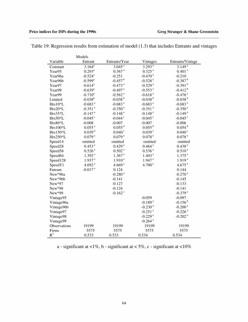
Price indices for ISPs during the 1990s Greg Stranger & Shane Greenstein _____________________________________________________________________________________________
64
Table 19: Regression results from estimation of model (1.3) that includes Entrants and vintages
Models Variable Entrant Entrants/Year Vintages Entrants/Vintage Constant 3.164a 3.045 a 3.293 a 3.149 a
Year95 0.293a 0.367 a 0.325 a 0.401 a Year96a -0.524a -0.251 -0.470 a -0.210 Year96b -0.599a -0.457 b -0.528 a -0.387 b Year97 -0.614a -0.473 a -0.529 a -0.391 b Year98 -0.639a -0.497 a -0.553 a -0.412 b Year99 -0.710a -0.562 a -0.618 a -0.476 a Limited -0.038b -0.038 b -0.038 b -0.038 b Hrs10*L -0.683 a -0.683 a -0.683 a -0.683 a Hrs20*L -0.351 a -0.350 a -0.351 a -0.350 a Hrs35*L -0.147 a -0.148 a -0.148 a -0.149 a Hrs50*L -0.045 c -0.044 c -0.045 c -0.045 c Hrs80*L -0.008 -0.007 -0.007 -0.006 Hrs100*L 0.055 a 0.055 b 0.055 b 0.054 b Hrs150*L 0.039 b 0.040 c 0.039 c 0.040 c Hrs250*L 0.079 a 0.079 a 0.078 a 0.078 a Speed14 omitted omitted omitted omitted Speed28 0.453 a 0.429 a 0.464 a 0.438 a Speed56 0.526 a 0.502 a 0.536 a 0.510 a Speed64 1.392 a 1.367 a 1.403 a 1.375 a Speed128 1.937 a 1.910 a 1.947 a 1.919 a SpeedT1 4.692 a 4.669 a 4.700 a 4.675 a Entrant -0.017 a 0.124 0.144 New*96a -0.280 a -0.270 a New*96b -0.141 -0.145 New*97 -0.127 -0.133 New*98 -0.124 -0.141 New*99 -0.162 c -0.379 a Vintage95 -0.059 -0.097 Vintage96a -0.189 a -0.156 b Vintage96b -0.230 a -0.200 a Vintage97 -0.251 a -0.226 a Vintage98 -0.229 a -0.202 a Vintage99 -0.264 a Observations 19199 19199 19199 19199 Firms 5575 5575 5575 5575 R2 0.533 0.533 0.534 0.534
a - significant at <1%, b - significant at < 5%, c - significant at <10%

Price indices for ISPs during the 1990s Greg Stranger & Shane Greenstein _____________________________________________________________________________________________
65
Table 20: Regression results from model (1.4) (includes new products and entrants)
Models Variable NewProducts New56k NewProducts
w/Entrants Constant 3.135 3.135 3.166 Year95 0.297 0.297 0.290 Year96a -0.305 -0.519 -0.314 Year96b -0.376 -0.590 -0.390 Year97 -0.398 -0.612 -0.424 Year98 -0.394 -0.608 -0.422 Year99 -0.458 -0.672 -0.486 Limited -0.040 -0.040 -0.041 Hrs10*L -0.676 -0.676 -0.677 Hrs20*L -0.343 -0.343 -0.344 Hrs35*L -0.141 -0.141 -0.141 Hrs50*L -0.038 -0.038 -0.039 Hrs80*L 0.000 0.000 -0.001 Hrs100*L 0.060 0.060 0.060 Hrs150*L 0.042 0.042 0.042 Hrs250*L 0.081 0.081 0.080 Speed14 omitted omitted omitted Speed28 0.239 0.453 0.241 Speed56 0.286 0.499 0.288 Speed64 1.179 1.392 1.181 Speed128 1.724 1.938 1.726 SpeedT1 4.471 4.684 4.473 New56 0.214 NewBoth 0.214 0.215 Entrant -0.019 Observations 19199 19199 19199 Firms 5575 5575 5575 R2 0.535 0.535 0.536
a - significant at <1%, b - significant at < 5%, c - significant at <10%

Price indices for ISPs during the 1990s Greg Stranger & Shane Greenstein _____________________________________________________________________________________________
66
Table 21: Regression results from model (1.5) (includes firm age and new products)
Models Variable Standard RE
Model (1.2) Firm Age
w/new products Constant 3.136 a 3.176 Year95 0.299 a 0.286 Year96a -0.516 a -0.333 Year96b -0.586 a -0.406 Year97 -0.590 a -0.439 Year98 -0.613 a -0.450 Year99 -0.684 a -0.528 Limited -0.038 b -0.041 Hrs10*L -0.682 a -0.677 Hrs20*L -0.350 a -0.344 Hrs35*L -0.147 a -0.142 Hrs50*L -0.044 c -0.039 Hrs80*L -0.007 -0.001 Hrs100*L 0.056 b 0.060 Hrs150*L 0.040 c 0.042 Hrs250*L 0.079 a 0.081 Speed14 omitted omitted Speed28 0.450 a 0.236 Speed56 0.522 a 0.283 Speed64 1.389 a 1.176 Speed128 1.934 a 1.721 SpeedT1 4.688 a 4.468 FirmAge 0.002 NewBoth 0.214 Observations 19199 19199 Firms 5575 5575 R2 0.532 0.536
a - significant at <1%, b - significant at < 5%, c - significant at <10%
Table 22: Estimated price premiums by firm age
Firm Age Beta*FirmAge Price Premium 1 Year 0.021 2.1% 2 Years 0.042 4.3% 3 Years 0.062 6.4% 4 Years 0.083 8.7% 5 Years 0.104 11.0%

Price indices for ISPs during the 1990s Greg Stranger & Shane Greenstein _____________________________________________________________________________________________
67
References
Aizcorbe A., C. Corrado and M. Doms (2000). Constructing Price and Quantity Indexes for High Technology Goods. Mimeo. Federal Reserve Board, Washington D.C.
Augereau, Angelique and Shane Greenstein. (2001) “ The need for speed in emerging communications markets: upgrades to advanced technology at Internet Service Providers,” International Journal of Industrial Organization, 19, pp 1085-1102.
Berndt, Ernst R. (1991), The Practice of Econometrics – Classic and Contemporary, Addison-Wesley. 1991.
Berndt, E.R. and Zvi Griliches. (1993) “Price Indexes for Microcomputers: An Exploratory Study.” In: M. Foss, M. Manser and A. Young, eds., Price Measurements and their uses, Studies in Income and Wealth, Vol. 57, University of Chicago Press, pp.63-93.
Berndt, E.R., Z. Griliches, and N.J. Rappaport (1995). “Econometric estimates of price indexes for personal computers in the 1990’s.” Journal of Econometrics, 68, pp.243-268.
Berndt, E.R., E.R. Dulberger, and N.J. Rappaport (2000). Price and Quality of Desktop and Mobile Personal Computers: A Quarter Century of History, Mimeo.
Gardner, James (1994). A DOS User's Guide to the Internet. PTR Prentice Hall. 1994.
Gordon, Robert J. (1989), “The Postwar Evolution of Computer Prices,” chapter 3 in Dale W. Jorgenson and Ralph Landau, eds., Technology and Capital Formation, Cambridge MA: MIT Press, pp.77-125.
Goldfarb, Avi (2002), “Concentration of Adv ertising-Supported Online Markets: An Empirical Approach,” mimeo, University of Toronto.
Greenstein, Shane (2001). "Commercialization of the Internet: The Interaction of Public Policy and Private Actions," in (eds) Adam Jaffe, Josh Lerner and Scott Stern, Innovation, Policy and the Economy, MIT Press.
Greenstein, Shane (2000). , "Building and Developing the Virtual World: The Commercial
Internet Access Market." Journal of Industrial Economics, December.
Greenstein, Shane (2000). “Valuing the net: What Det ermines Prices for Dial-up Internet Access?” Working Pape r, Northwestern University.
Griliches, Zvi (1961), "Hedonic Price Indexes for Automobiles: An Econometric Analysis of Quality Change," originally in The Price Statistics of the Federal Government, New York: NBER, 1961.

Price indices for ISPs during the 1990s Greg Stranger & Shane Greenstein _____________________________________________________________________________________________
68
GVU’s WWW User Survey, Surveys 3 -10. http://www.cc.gatech.edu/gvu/user_surveys/ Graphics, Visualisation and Usability Lab. Georgia Institute of Technology. Atlanta: 1995-1998.
Krol, Ed, (1992). The Whole Internet. O'Reilly & Associates, Inc. 1992.
Krol, Ed (1994). The Whole Internet - 2nd Edition. O'Reilly & Associates, Inc. 1994.
Marine, April, Susan Kilpatrick, Vivian Neou and Carol Ward (1993). Internet: Getting Started. PTR Prentice Hall. 1993.
Meeker, Mary and Chris Dupuy (1996). The Internet Report. Harper Collins Publishers, Inc. 1996.
Prud’homme, Marc and Kam Yu (1999). Towards an Elementary Price Index for Internet Services. Unpublished manuscript – Statistics Canada. 1999.
Raff, Daniel M. G. and Manuel Trajtenberg (1997), “Quality -Adjusted Prices for the American Automobile Industry: 1906-1940,” in (eds) Timothy Bresnahan and Robert Gordon, The Economics of New Goods, University of Chicago Press, Chicago, 1997.
Sachs, David and Henry Stair (1994). Hands-On Internet. PTR Prentice Hall. 1994.
Schneider, Karen G (1996). The Internet Access Cookbook. Neal-Schuman Publishers, Inc. 1996.
Smart Computing® Dictionary (2000). PC Today.com. Sandhills Publishing Company. 2000.
Triplett, Jack (2000). “Index Numbers.” New Palgrave Dictionary of Economics
Triplett, Jack E. (1989), “Price and Technological Change in a Capital Good: A Survey of Research on Computers,” chapter 4 in Dale W. Jorgenson and Ralph Landau, eds., Technology and Capital Formation, Cambridge MA: MIT Press, pp.127-213.
Varian, Hal and Carl Shapiro (1999). Information Rules: A Strategic Guide to the Network Economy. Harvard University Press. 1999.