Prices, Price Indexes and Poverty Counts in India during ......Prices, Price Indexes and Poverty...

Paper 1

Prices, Price Indexes and Poverty Counts in India during 1980s and 1990s: Calculation of UVCPIs1

Abstract This is the first part of three papers in which we revisit issues surrounding poverty calculations in India during the 1980s and 1990s. A number of recent papers have put forward or endorsed poverty calculations based on poverty lines computed using Unit Values (expenditure divided by quantity) of food, and fuel and light items in the National Sample Survey Consumer Expenditure Surveys, which they suggest are more plausible than those produced by the Indian Planning Commission. Others have criticised a growing gap between money-metric poverty based on poverty lines and food poverty based on normative calorie consumption levels.

In this first paper we explore the use of Unit Values to compute Consumer Price Indexes (UV CPIs). In the second paper we discuss whether it is reasonable to use these UV CPIs or other available CPIs to compute poverty lines for different geographical and temporal domains from a single base PL, or to base poverty lines on calorie norms. In the third paper we explore the poverty counts that result from our “best” approach to poverty lines and compare them with those from “robust” poverty comparisons and other indicators of well-being..

In this paper we show that (i) the UVs calculated from the National Sample Survey (NSS) Consumer Expenditure Surveys (CES) are multi-modal corresponding perhaps to different prices being paid by different population groups, for different qualities of produce, or at different times or places; (ii) UVs vary within states (specifically by the National Sample Survey Regions (NSSR)), by expenditure group, and by town size within the urban sector; (iii) UVs do not always correspond well with prices used by the PC for its poverty line calculations; (iv) the differences between rural and urban CPIs that are reported both by the PC and by other researchers are not soundly based; (v) neither alternative methods of computing UVs nor alternative methods of computing CPIs from UVs overcome the problems identified. We argue that UVs computed from household expenditure surveys can be a useful check on prices obtained from markets and by quotation that are generally used in computing price indexes. But they are no substitute for proper price data required for CPI calculation. However, current practices of price collection and CPI calculation in India need to be thoroughly overhauled, in part because they are based on long out of date sampling schema which cannot now assess the differences in costs of living in different domains and for different social groups.

1 Amaresh Dubey, North Eastern Hill University, Shillong and NCAER, New Delhi) and Richard Palmer-Jones (corresponding author), University of East Anglia, [email protected].

Forthcoming Arthavijnana

1

Acknowledgement: We gratefully acknowledge the helpful comments of an anonymous reviewer in substantially improving this paper. The work on which this paper is based was largely funded by the projects R8256 of the Social Science research Committee of the Department for International Development of the UK Government. Dr. Kunal Sen and Professor Ashok Parikh of the University of East Anglia were collaborators in this project. Though in the study we carried out this exercise for both India and Bangladesh, in this paper we discuss the issues surrounding Indian debates; work on Bangladesh will be reported elsewhere. Access to official price data was provided by Officials at Labour Bureau, Shimla. Data from the 38th, 43rd and 50th Rounds of the NSS were made available by NSSO under the collaborative agreement between the Overseas Development Group and the NSSO. The views put forward here are not necessarily endorsed either by DFID or the NSSO, or indeed by our collaborators.


Paper 1

Prices, Price Indexes and Poverty Counts in India during 1980s and 1990s: Calculation of Unit Value Consumer Price Indexes

1. Introduction In the five decades since the inception of the Indian Republic there is hardly any issue of public policy and opinion has been so controversial as the incidence of poverty. Without doubt, a clear understanding of poverty levels and their trends in the different regions and among the different population groups in India has profound implications for government policy not only there but among developing countries more generally for whom the Indian experience has been exemplary.

Estimating poverty employs poverty lines and aggregators1. In the international literature surprisingly little attention has been paid to poverty line (PL) calculations (pace Lanjouw, 1999) given their significance in determining poverty assessments2 3. In India on the other hand, there is a considerable history, including much methodological innovation, of debates about appropriate poverty lines, including the seminal contributions of Dandekar and Rath (1971a & b), and the Task Force (GOI, 1979) and the Expert Committee set up by the Planning Commission (PC) (GOI, 1993), to establish official PLs, both of which comprised distinguished academics and poverty experts. Moreover, recently PLs in India have been the subject of some controversy (Deaton and Tarrozi, 1999; Deaton and Kozel, 2005). We do not discuss the evolution of these debates, which are well surveyed in in the references given and elsewhere (e.g. Rath, 1996; Rath, 2003). Further, we focus on the use of Unit Values in the calculation of PLs and orthodox methods of computing Consumer Price Indexes4 and poverty lines, and do not discuss other methods of computing CPIs or PLs except in passing5.

The poverty aggregates and PLs currently used by the PC have been criticised from a number of perspectives, including the apparent contradiction between mean consumption estimated in the CES and the national accounts (Bhalla and Das, 2004; Ravallion, 2003),

1 Poverty lines will vary spatially and temporally; they should also vary by size and composition of households, and perhaps also by social group to account for the socially determined components of necessary consumption. 2 Such a judgement is perhaps controversial. We would just point out that the World Bank’s premier expert on poverty measurements first book length contribution emphasises aggregation much more than poverty line (Ravallion, 1992, 1994), and the later contribution on Poverty Lines (Ravallion, 1998) is much thinner. 3 This is not just because there is generally no natural cut-off point in the distribution on expenditures or incomes which can serve as an uncontroversial dividing line between the poor and the non-poor (Deaton, 1997). 4 What are known as atomistic or functional methods rather than stochastic methods (Selvanathan and Rao,1994). 5 However, we argue that no methods based on UVs escape the problems and issues we identify. We do not discuss calorie based PLs in detail, except, in the second paper in this series, to point out that they suffer similar problems to those we identify in (UV) CPI based PLs.


1

and the gap between calorie consumption at the poverty line and the calorie norms in which these PLs were originally anchored (Vishwanath and Meenakshi, 2003, Patnaik, 2004; Ray and Lancaster, 2005). We touch on these issues, particularly the latter, below and in the other two papers; in this paper we discuss the use of UVs to compute new CPIs.

Several authors have calculated UV based CPIs for different states or regions in India (Rath, 1973; Chatterjee and Bhattacharya, 1974; Bhattacharya et al, 1980)6. However, for the most part these have been methodological papers rather than attempts to recalculate poverty, and have not suggested replacing the official poverty lines and counts with their own. However, recently Deaton and Tarrozi, 1999 (D&T), and Deaton (2003a), have argued that the official poverty lines (OPL) used by the Indian Planning Commission (PC) are suspect on both methodological and empirical grounds. D&T argue that the base year (1973-4) PLs are derived in a convoluted manner from different fairly arbitrary calorie norms for rural and urban areas7 and consumer price indexes. They also suggest that the consumer price indexes for agricultural labourers (CPIAL) and for industrial workers (CPIIW) used to update PLs are unsatisfactory Laspeyres indexes using long out-of-date base weights8.

D&T computed Unit Value CPIs and applied them to the all India official rural poverty line for the 43rd Round (OPL43r) to obtain new PLs. Their UV CPIs were computed from the 43rd and 50th Rounds using Unit Values (expenditure on an item divided by quantity bought), and democratic average budget shares for the whole population as weights. Deaton, 2003a, extended these UV CPIs, PLs and poverty counts to the 55th Round. The D&T PLs have been used by others (e.g. Kijima and Lanjouw, 2003), and received some endorsement from Sen and Himanshu (2004a, 2004b), and in a recent contribution by Besley, Burgess and Esteve-Volart (2005). These and other issues related to poverty calculations are discussed quite extensively in Deaton and Kozel, 2005a & b. However a number of concerns can be raised about these UV CPIs and the PLs computed from them, which we explore in this and the following papers.

Like others we use the household level consumption expenditure data collected by the National Sample Survey Organisation (NSSO); our calculations cover the four quinquennial rounds (1983, 1987-88, 1993-94 and 1999-2000). Thus we replicate and extend Deaton’s series back to the 38th round using our own variations on his method9. 6 Coondoo et al., 2004, compute indexes based on unit values, but only to illustrate a method, and for four regions rather than individual states of India as in the other poverty calculations discussed here. 7 These calorie norms are derived from international standards and their translation into expenditure levels is made using a food energy intake method. However, below in this paper and in the second paper in this series we argue that this method cannot establish levels of expenditure in different domains that corresponds to the same (poverty) level of welfare. 8 There had been concern with methodologies of CPI calculation in recent years in developed countries as well, especially the USA (Moulton, 1996; Boskin, et al., 1998; Deaton, 1998). 9 Thus we focus on bilateral CPIs using individual observations on UVs and average budget shares (AVBS) using the All India Rural sector as the base; we discuss only briefly stochastic methods of computing CPIs using, for example, the multilateral CPIs by the method proposed by Eltetö and Köves (1964), and Szulc(1964) (EKS), or a variant of the Country Product Dummy (CPD) approach proposed by Rao (1990) . The stochastic approach to multilateral CPIs is also discussed in ILO, 2004:299-304.


2

Further, we calculate price indexes for NSS Regions (clusters of districts within states10) as well as all India and major states, rural and urban sectors, and for towns of different size.

The rest of the paper is organised as follows. In the next section we provide a brief review of the PL calculations of the PC and the methodology of UV CPI calculations as used by D&T. This is followed in section 3 by discussion of our UV CPI calculations and problems associated with them. In section 4 we report and discuss our UVs and UV CPIs and compare some of them with prices used in the CPIAL and CPIIW. Section 5 concludes the paper.

2. Unit Value Based Consumer Price Indexes In this section we first discuss the derivation of Official Poverty Lines, and the UVs used in CPIs employed in PL calculation. Then we look at the effects on UV CPIs of different levels of aggregation, by state, expenditure group, and size of towns.

Current Official state (and all India) Poverty Lines derive from the Task Force (GOI, 1979); they are anchored in the base year (1973-74) all India Rural and Urban poverty lines derived from separate calorie norms and computed by a food energy intake (FEI) method.

These 1973-74 PLs are adjusted for state differences in prices using “Fisher” state price indexes for 1973-4 derived from (Fisher) UV deflators computed11 for each state by Chatterjee and Bhattacharya, 1974, using 1963-4 NSS data; these CPIs are adjusted to 1960-61 and updated from 1960-61 using State Consumer CPIAL and CPIIW (GoI, 1993:74). Subsequently, these base PLs have been updated using state/sector CPIs - CPIAL for the rural sector and CPIIW for the urban sector (GOI, 1993)12. The items included in the original State deflators calculated by Chatterjee and Bhattacharya (1974), as with other UV CPIs, constitute only a fraction of household expenditure.

D&T (see also Deaton, 2003a) asserted that the OPLs for some states relative to others are not consistent with common knowledge. They also argue that the Indian urban OPLs are “outrageously” out of line with real urban-rural differences in the cost of living. Further, following the main conclusions of index number theorists, D&T argue that the between Rounds OPLs based on Laspeyres indexes with long out of date base weights are unreliable. They go on to compare Official CPIs with Unit Value CPIs they computed from the Indian National Sample Survey Consumer Expenditure Surveys. As noted above, these UV CPIs are computed using a subset of items reported in these surveys for which “Unit Values” (expenditure on item divided by quantity of item purchased) can be

10 See Murthi et al. (2001), for the NSSR within States and a mapping of Indian districts to NSSR. 11 i.e. CPIs computed using UVs and average budget shares from the NSS CES. 12 We have been able to replicate the Lakdawala Report calculations using readily available sources; details of these calculations that give approximately the same results as published in the Lakdawala Report Appendix Tables AIV.9 and AIV.10) can be obtained from the corresponding author.


3

sensibly computed; democratic average budget shares (AVBS)13 are used as the CPI weights14.

The NSS and many other household expenditure surveys conducted in developing countries report both the quantity purchased and total expenditure on a large number of items covering, in the Indian case on average about 70 percent of total household expenditures. D&T compute UV CPIs for each major Indian state for the 43rd and 50th rounds using the Laspeyres, Paasche, Fisher and Tornqvist formulae15. D&T (and Deaton, 2003a) then compute PLs by applying their Tornqvist CPIs to the all India Official Rural Poverty Line for the 43rd Round (OPL43r)16; these PLs showed spatial patterns (inter-state and urban/rural differences) and temporal trends that were different from those implicit in the OPLs. These new poverty lines featured in a number of contributions to a World Bank sponsored conference on poverty measurement in India in Delhi in January

13 It is common for average budget shares (say on item i) to be computed in a “plutocratic” manner by dividing expenditure by all households on an item i by expenditure on all items by all households; this means that the average is implicitly weighted by expenditure. Democratic budget shares are computed as the average of average budget shares; in this case each observation is weighted by household size so that each household’s expenditure counts equally. 14 In the quinquennial NSS surveys up to and including the 50th, two sets of columns are provided to report expenditures and quantities; one for purchased items the other for consumption out of home produced items. A third pair of columns is for total consumed. The totals may not be the sum of purchased and consumed out of home produced columns because some purchased may be stored or there may be consumption out of stocks. There are well known difficulties with valuing home produced goods as the values have to be imputed. Various strategies can be employed to compute UVs, including using all three columns, using only the purchased items column, using only the purchased and home produced columns, or using only the totals column. In our calculations we have used only the totals columns; there is something to be said for using the purchases columns in preference to the Totals columns since the home produce expenditure column have been imputed. However, this would rule out quite a number of households which do not purchase. In the vast majority of cases the Totals columns give the same UVs as the Purchased columns where there are data in both Purchased and Home Produced Columns. Most divergences seem to be due to data entry problems. Budget shares must be computed from the Totals columns. 15 The NSS data set includes a monthly per capita expenditure (MPCE) aggregate that can be used as the denominator for AVBS calculations. It is possible to recalculate MPCE from the data on all items reported; we find that our recalculations of MPCE do not always match the figures given, however the differences are small. Given that D&T screen UVs for extreme values it is not clear whether MPCE should be recalculated after excluding those extreme UVs which are dropped in the calculation of the UVCPIs. We have experimented with recalculating MPCE imputing median UVs in place of extremes, and with various strategies for adjusting weighting schemes if data for individual households have to be dropped because of implausible quantities or expenditures. It is not clear that the rather minor differences that results are worth the effort, and they are not reported here. A major problem is to decide whether extreme UVs are the result of errors in the expenditure or the quantity variable. In the longer run a more appropriate way of dealing with problematic values is needed but this is beyond our resources. 16 First the State rural vs all India UV CPI is applied to the OPL43r; then the state urban vs rural UV CPI is applied to the state rural PL. Inter-round inflation uses the all India rural CPI for the next round vs the preceding round applied to the OPL43r and its successor, and the state rural and urban PLs are computed by applying successively the state rural vs all India CPI and the state urban vs rural CPI.


4

200217, the papers from which have been edited in to a book (Deaton and Kozel, 2005b; see also Economic and Political Weekly, 2003, January 25th).

Most calculations of poverty in India have been made at state and sector level; however states are extremely diverse (Vaidyanathan, 1992; Dreze and Srinivasan, 1996; Dubey and Gangopadhyay, 1998; Palmer-Jones and Sen, 2003, 2006), raising the question of whether poverty should be calculated for more homogenous areas within states, such as the NSS Regions (NSSR)18. Consequently, heeding the critique of OPLs, and in the absence of viable alternatives, we compute UV CPIs and poverty for the 38th and subsequent quinquennial Rounds, for the rural and urban sectors within NSSR (as well as for states), and for towns of different size19. In addition we computed UV CPIs for each quartile of the expenditure distribution (q1, q2, q3, and q4), and quartiles 2 and 3 together (q23), as well as the whole population (in each sector). That is we calculate:

(a) each round on the preceding round for the all India rural sector (UVCPIair

t0,t1);

(b) within round state (and NSSR) rural and urban vs all India rural and urban UV CPIs (UVCPIsr,air

t and UVCPIsu,aiut);

(c) within state urban vs rural UVCPIsu,srt

(d) state urban and townsize vs all India urban UVCPIsu,aiut;

(e) Round on Round All India, State sector and NSSR deflators.

Our results together with critical comments on UVs and UV CPIs are briefly described below20. It was during this work that we became increasingly doubtful of the use of UVs in CPI calculation, and these doubts are the main topic of this paper.

2.1 UV CPIs at State Level We begin by discussing the state level UV CPIs. Figure 1 compares our UV CPIs with the CPIs implicit in the OPLs and those computed by Deaton and Tarozzi (1999) and Deaton (2003a), and Maps 1 and 2 give the OPL and UV CPIs in spatial context. Our State UV CPIs for the 38th, 43rd, 50th and 55th Rounds are quite well correlated with D & T’s for the rural sector but differ somewhat in the urban sector (Figure 1 and Table 1). Both our and Deaton’s UV CPIs differ significantly from the implicit OPL state vs all India deflators.

Turning to round on round inflation, Figure 2 shows the associations among inter-round CPIs (Table 2 gives the correlations). It is again clear that our figures are close to 17 Which also covered many other topics, especially the implications of the design changes in the 55th Round. 18 NSSR are groups of districts within states used by the NSSO in its sampling schema. 19 We are most grateful to Angus Deaton for providing sample STATA code that he used to compute UVs, AVBS and CPIs. Using this code not only helped us understand the D&T method exactly, but also to learn Stata. We have changed this code substantially and do not always get the same results as D&T report where we can compare them, although the results are generally very similar. 20 Results not reported here (e.g. by NSSR) can be obtained from corresponding author.


5

Deaton’s and both ours and Deaton’s are lower than the OPL inflator for the 43rd to 50th and 50th to 55th rounds. But our deflators for the 38th to 43rd rounds are not generally lower than the implicit OPL deflators (Table 3). For some states the OPL inflation is significantly larger than ours (43-50th rounds – in the rural sector Haryana, Himachal Pradesh, Madhya Pradesh, Rajasthan, and Uttar Pradesh); in the urban sector our inter-round deflation CPIs are closer to Deaton’s than to the OPL although there is more variability. For the 50th – 55th Rounds inflation, our and Deaton’s rural deflation factors are not significantly correlated with the OPL implicit deflators.

For the rural sector the minor differences between our State UV CPIs and Deaton’s suggest that small adjustments to data cleaning rules and programming of UV and AVBS calculations can make differences to the UV CPIs that are calculated from these sources. Our findings confirm the argument that the implicit CPIs in the OPL for Rural AP relative to all India may be much too low. Interestingly, the bilateral CPIs computed by Bhattacharya et al (1980), also do not show as low a value for AP in 1973-74 as reported in the Expert Group (Lakdawala) Report21.

In the urban sector the results are very variable reinforcing the conclusion that small differences in data processing (and perhaps data, since we have found that different versions of the same data from NSS are not always identical) can make significant differences to UV CPIs. Deaton argues that the official urban poverty lines are too high, but this does not arise because the urban UV CPIs are low relative to the implicit deflators calculated from the OPLs. Table 4 reports our urban vs rural CPIs which broadly correspond to those calculated by Deaton (2003:364 (Table 3), and to the implicit urban vs rural CPIs of the OPLs. Bhattacharya et al. (1980) also found smaller differences between urban and rural price levels (16 percent) than are implicit in the OPL deflators. Hence, Deaton’s conclusion about the gap between urban and rural PLs arises not from different CPIs but from the way the PLs are calculated from a common base poverty line. This is discussed in the second paper in this series where we argue that Deaton’s method of calculating urban poverty lines is also inappropriate22.

21 State CPIs have been calculated by Maitra (1959), Rath, (1973) for 1961-2, and Coondoo and Shaha, (1990), in addition to those mentioned above. Lakdawala shows a “Fisher” index for rural AP of 85.11 (relative to all India) for 1973-4; Bhattacharya et al (1980) who report Laspeyres, Paasche and Fisher indexes using the 28th Round of the NSS (1973-4) give the All India v AP (rural) Fisher index of 111.64, which is 89.6 for the reverse comparison. Coondoo and Shaha (1990) use the 1963-4 state Fisher indexes (from Chatterjee and Bhattacharya, 1974), and state CPIALs to calculate bilateral indexes for various years. Using their rural 1983-84 bilateral indexes for the 38th Round to calculate “EKS” multilateral indexes (the average over states of bilateral Fisher) indexes, AP ranks 11th out of 14 states rather than the bottom as in the Official Poverty Lines of the Expert Group (Lakdawala) Committee (GOI, 1993). 22 While the CPIs of urban vs rural domains may err because only items for which UVs can be calculated are included in the indexes, a problem that is common to all UV methods, this is only one problem. The problem we identify with Deaton’s method of computing urban PLs, in a nutshell, is that a base rural PL multiplied by an urban vs rural CPI probably underestimates the cost of living required in urban areas to achieve the standard of living of rural households corresponding to the rural PL, because more goods and services have to be paid for in urban areas that can be obtained free or at much lower cost in rural areas. Housing is a typical example that is (a) excluded from the UV CPIs, and (b) hardly figures in rural household expenditures, but is s significant component of urban household expenditures.


6

2.2 UV CPIs at NSS Region Level Following Dubey and Gangopadhyay (1998) and Palmer-Jones and Sen’s (2003) emphasis that poverty varies within states, we have extended the D&T approach to calculate UV CPIs for NSS Regions, for rural and urban sectors, and for towns of different size within the urban sector (within NSSR). Table 5 shows, for the rural sector of selected states23, that UV CPIs do vary within states by NSSR, and that there is considerable consistency between rounds as shown by the ranks of regions with states over rounds, especially in the rural sector. Moran’s I, a measure of spatial autocorrelation (Anselin, 1988), shows clear spatial autocorrelation of rural UV CPIs across regions, but not for urban sector except for the 43rd Round. This suggests that markets for consumer items may be more integrated in urban than rural sectors24.

These findings reinforce arguments that NSSR are the more appropriate unit for the design and assessment of policy (Palmer-Jones and Sen, 2003, 2006). Further work is needed on the grouping of NSSR across states, and on reassessing the geographical units from which NSS constructs samples and analyses of their data so as to better represent spatial variation in prices and expenditure patterns.

2.3 UV CPIs by Economic Status We have also computed UV CPIs for different quartiles of the expenditure distribution; we give results for all India only (Table 6) but very similar patterns are observed for all states and NSSR. There are significant differences in UV CPIs for different expenditure groups, with the UV CPI generally somewhat lower for the lower than the upper quartiles especially in the 50th and 55th Rounds (Figure 2). Inter round inflation also varied between groups but the pattern is not constant over time; only between 43rd and 50th rounds is inflation rate of the poorest quartile much less than that for other groups, while the reverse is true between the 50th and 55th rounds (results available from the authors). The differences in UV CPIs by expenditure group depended on both differences in expenditure patterns (AVBS) and on different patterns of UVs.

2.4 UV CPIs by Size Class of Towns It is evident to anyone acquainted with India that larger cities especially metropolises have very different costs of living compared to smaller towns of the hinterland. This is recognised, for example, in the dearness allowances for government servants and is confirmed by our calculations of UV CPIs for towns of different size within the urban sector (Tables 7 and 8, Figure 3). The effects of computing poverty by town size are discussed in the third paper in this series.

23 States in this tables have not been selected for any particular reason; full results are available from the authors 24 We have not computed spatial autocorrelation for towns of different size; given that small towns have CPIs close to those of the rural sector of the NSSR within which they fall (see below) it is possible that CPIs for small towns also show spatial autocorrelation.


7

3. Treatment of Non-Unit Value Items UVs can only be calculated for a subset of items which households consume, and this is a serious limitation to the construction of CPIs from them25,26. UVs are generally calculated for food and fuel and light items only. Although UVs can be calculated for some footwear and clothing items this was not done by D&T, or ourselves, although Bhattacharya et al. (1980), included clothing in their UV CPIs. D&T comment that there are likely to be quality differences (spatially and over time) for these items rendering them inappropriate for CPI construction27. We term items included in UV CPI calculations UV items, and items excluded from these calculations, non-UV items.

The proportion of total household expenditure reported in NSS surveys for which UVs can be computed varies from less than 50 percent to over 80 percent UV items are a significantly higher proportion of household consumption in rural than urban sectors28. D&T assume that the prices of items not included in the UV CPIs do not differ spatially or inflate at a different rate to UV items. This is clearly an arbitrary assumption which, although made explicit, is likely to arise because of lack of access to relevant data rather than because it is valid. As shown below it is possible to use other data to substitute this assumption, and, as discussed below, what other data are available suggest that it is 25 There are many other problems in using data from household expenditures in the third world that we do not explicitly address; often mentioned is that much consumption is from home produced goods for which expenditure has to be imputed. We do not mention this further here although it obviously has relevance to the use of UVs of these items. Deaton and Zaidi, (2002) provide an illuminating discussion in the context of the World Bank Living Standards Measurement Studies (LSMS); Deaton and Grosh (1999) are also instructive. In neither case, however, is one convinced that adequate attention is paid to field data production problems, such as the respondent fatigue reported by the field operations by the NSS section responsible for field data collection (NSSO, 2003). 26 NSS does not impute consumption from household assets, including owned housing, and includes the whole expenditure on all durables. This makes the total expenditure aggregate and budget shares somewhat unreliable for poverty analysis. 27 It is not clear that quality differences do not afflict items included in the UV CPI calculations, for example many food items have significant quality variations, even the staple rice. We show below that there are likely to be quality differences within food items, associated positively with expenditure per capita. In later work we intend to explore the unit values of some items of footwear and clothing. Elsewhere Deaton has an instructive discussion of quality issues in UVs calculated from NSS data (Deaton, 1997; Deaton et al. ,1994) 28 One must distinguish the share of UV items actually included in the CPI from the share of the groups of commodities for which UVs are calculated – in the Indian NSS CES surveys these are Block 5 items - since some of these items are excluded from the CPI because there are too few observations in the base or comparison domain, or because they differ so greatly between domains as to be based on different units or be otherwise non-comparable (in some cases corrections can be made, for example for obvious decimal place errors). Our screening eliminates items where the difference in UV between domains is greater than 30 percent for within round comparisons, and greater than 300 percent % between rounds, as well as when there are fewer than 20 observations (for town size CPIs within NSSR we used 10 observations as the cut off because of the small number of observations of less frequently consumed items) in either domain. Thus, in fact, two assumptions are needed – first that UV items not included in the UV CPI inflate at the same rate as the UV items included in the CPI, and secondly that the non-UV items (Blocks 6-9) also inflate at the same rate. UV items included in the UV CPIs are generally over 95 percent of expenditure on UV items, but since the excluded items are likely to be “exotic” there is no reason to think that they will follow the same price trends as those included UV items.


8

erroneous to assume that UV and non-UV items have the same spatial or temporal inflation rates.

To adjust the round to round indexes for the inflation of non-UV items we experimented with augmenting the all India UV CPIs using official all India non-UV group indexes29 from the CPIAL and CPIIW, and the all India expenditure share of UV items as weights30. The CPIAL and CPIIW data for the years 1983, 1987-88, 1993-94 and 1999-2000 corresponding to NSS survey years, are the data from which we have calculated these indexes. There are some qualifications to our actual calculations based on limitations in our data as described below:

1. there are no separate indexes for different monthly per capita expenditure groups, so we have used the same non-UV indexes for all groups. The weights with which these non-UV indexes are compiled probably represent expenditure patterns of agricultural labourers and industrial workers with a considerable lag; the latter in particular may not represent the poor who are often in the informal sector;

2. the CPIAL and CPIIW indexes changed their base in the middle of our period (from base 1960-61=100 to 1986=100 and 1982=100 respectively) and the linking factors have always been rather obscure;

3. the CPIIW indexes are for centers, the number and composition of which changed between the old and new base series. We have aggregated over centers within states using the center weights to produce item group CPIs by state. The CPIAL data are compiled at state level only;

4. we do not have separate item group weights for states for the earlier base indexes, so we have had to assume the same state group weights for the earlier rounds as in the later rounds, and for centers which were dropped from the later base indexes we used the state average weights;

5. the later period new base CPIIW separated housing from the miscellaneous group; we have aggregated the housing index into the miscellaneous using their respective weights;

6. the CPIAL does not have state group weights, or group weights for the earlier series (that we have been able to find); we use the later series all India group weights;

7. the CPIAL has both state linking factors and all India group linking factors – we have used the all India group linking factors.

29 . There are 5 or 6 subgroups of items whose indexes are combined to produce the CPIAL and CPIIW; these are food, pan, supari, tobacco and intoxicants, fuel and light, clothing, bedding and footwear, and Miscellaneous. The housing was split from the miscellaneous category in the new series (covering 50th and 55th Rounds). The General Index is the combined CPI. We used the non-food and non-fuel and light indexes for the non-UV items indexes. 30 Too much uncertainty attaches to the validity of this procedure to warrant a detailed presentation of the data.


9

3.1 State Differences in UV and non-UV Group Indexes There are some differences between states in the UV and non-UV sub-group indexes (Figure 4 shows these differences for the CPIAL). This suggests that we cannot assume that UV and non-UV items will inflate at the same rate even though, given the different basis of official price indexes and UV CPIs, this is not direct evidence to this effect. We have not analysed these figures, but it would be useful to compare the non-UV items indexes with (a) Unit Values for footwear and clothing items for which UVs can be calculated from the NSS CES, and (b) with selected non-food items that are published for states (rural) or centers (urban) in the Indian Labour Journal and elsewhere to check the D&T assumption of equal indexes for UV and non-UV items.

3.2 Inter-round non-UV Inflation The non-UV sub-group index inflated faster over the period as a whole than the UV sub-group index for both CPIAL and CPIIW (Figure 5); between the 50th and 55th Rounds the UV sub-group in the CPIAL did inflate relatively faster (Figure 5) although this was not the case in all States

Table 8 reports the synthetic CPIs computed as weighted averages of the UV CPIs and the non-UV group indexes of the state CPIAL and CPIIW using the computed budget shares as weights31. These non-UV group indexes are of course based on long out of date base weights, and, from what we can see of the data that are used in the construction of these indexes, collected from the Labour Bureau Shimla, there are likely to be many problems of missing data, sampling, data processing and so on. Exposure of these data to greater public scrutiny might lead to improvements in their quality.

4. Unit Values and Market Prices The UVs calculated from the NSS consumer expenditure surveys are not prices of constant utility (pure) commodities; UVs are affected by the characteristics of the commodity actually purchased such as location, bulk, quality, packaging, branding, and so on. Prices used in official CPI calculations refer to standardised commodities with uniform characteristics at specified locations and times. Market price surveys are supposed to control for these other characteristics by, for example, using a single quality of commodity, at a given location, and fixed quantity so as not to confound changes in prices with changes in utilities32. Unit Values are not controlled in this way, and are likely to be associated with characteristics of the household, in particular its expenditure since,

31 These are the shares of all UV items whether included in the UV CPI or not – e.g. including UV items that were excluded from the UV CPI calculations because there were less than 20 (sometimes < 10) UVs in either the base or comparison unit, or because the difference in computed UVswas deemed excessive (see above). It is assumed that the computed UV CPI is a better indicator of the price difference for these excluded items than the non-UV CPI. 32 E.g. a given rice variety sold loose by the kilogram in a given market, often at a fixed day of the week and time of day. Even this specification is not implementable because the qualities of rice and the locations and forms in which it is sold vary with the seasons, and have changed over time. Nevertheless, official price recording procedures have detailed specifications for these contingencies.


10

as incomes/ expenditures rise, characteristics other than nutritional content are likely to become more important33.

4.1 Unit Values as Prices D&T use the median Unit Values for the whole population. Others, such as Wodon (1997) and World Bank (2002) use a regression of UVs on a set of household characteristics and area dummies to estimate UVs typical of the poor. These are typical Prais “quality” regressions widely used in consumer survey analysis (Prais and Houthakker (1955); Deaton (1997); Coondoo et al. (2004)). It is not clear that either of these approaches results in Unit Values that are appropriate for the calculation of CPIs for the poor. Median values are typically justified as being more robust to outliers than the mean, while the regression method is justified as more likely to result in UVs representative of those paid by the poor:

“One may be tempted to simply estimate the mean unit values for the various food items by geographical area, but this may yield biased estimates of the food prices encountered by the poor. For example, if the quality of the food purchased is a normal good, the mean unit values will tend to increase with the mean consumption level of the households. Then, at the aggregate level in each geographical area, a rise in the standards of living of, say, the better-off will raise the mean prices of food, and thereby the food poverty line. If the poor keep buying lower level food items whose price may not have risen, the estimated poverty line will result in an overestimation of poverty. Also, if other characteristics of households differ by geographical areas, the estimated mean unit values will be affected by these characteristics, and they will not accurately represent the food price differentials confronted by poor households in different areas. Once again, we will lack an adequate index of the relative area price differences.” (Wodon, 1997).

We argue that neither method is satisfactory; nor are we convinced that an alternative method such as quantile regression (Wagner, 1959; Narula and Wellington, 1982) does not also fail to capture important features of the distributions of UVs such as clustering on specific values (see below).

4.2 Median UVs UVs of many commodities are not continuously distributed but clustered, generally on whole numbers. Figures 6a and 6b show the unit values for rice and wheat respectively in different states in the 55th Round, clearly clustering on specific values, a significant proportion of which are different from the median. Figures 6a&b also show the prices used in the construction of the OPLs, showing in many cases significant differences from the median Unit Values. This raises questions as to the appropriateness of the official price collection processes. It will not always be the case that UVs are a good check on the 33 Notwithstanding the common claim that the wealthy can purchase in bulk and hence obtain better prices, UVs invariably rise by expenditure per capita class, because the rich are buying better quality in more valued environments, and so on.


11

official prices, but where different states show significantly different divergences between UVs and “official” prices (i.e. prices computed from market surveys or price quotations) then there must be concern whether official procedures for collecting prices are focussing on the appropriate qualities and outlets for these items in the states which show significant divergence with UVs.

4.3 Regression based UVs34 Wodon (1997) describes the regression method of computing “prices” appropriate for calculating spatial poverty lines (which is the same as that proposed by Chen and Ravallion (1996)) as follows:

“To compute prices controlling for households characteristics, we defined for household i the unit value for the food category j as Pji = Vji/Qji, where Qji is the quantity purchased and Vji is the value of the consumption for item j. Following Chen and Ravallion (1996), for each food item j, we then regressed the unit values against area dummies and household characteristics35:

Log Pji= α+ βij log (Yi/n,)+β2j [log (Yi/n,)]2+δ’Di+T’jXi+ π’jWj+ Ω’jEj+ε (4.1)

where Y, is the consumption expenditure of the household, ni is the household size, D is a vector of dummy variables for the geographical areas, W is a vector of dummy variables for the highest education level among the members of the household, X is a vector of dummy variables for the employment status of the head of the household, and E is a vector of demographics. We have excluded from the computation of the total expenditures for each household the amount spent on ceremonial activities for marriages and funerals as these tend to be non-recurrent. The regression coefficients on the area dummy variables can be used to estimate the differences in food prices purged of quality differences. The expected food price paid for item j in area k by a household with the characteristics corresponding to the omitted dummy variables in the unit Values regressions will be Pjk = exp(δjk) Pjr where Pjr is the median price in the reference area omitted in the regression ….. Two points should be mentioned here. First, the omitted dummies in the regression should be representative of the poor. In our analysis, we excluded the dummy variables corresponding to illiterate and landless or near landless household heads working in the agricultural sector. Second, because the prices of the reference area Pjr carry

34 While this method has not been applied to compute new PLs for India it has for Bangladesh. However, it is appropriate to deal with it here as it may be put forward as a way of overcoming problems with other methods of computing UVs. 35 An anonymous reviewer has pointed out that this model is likely to suffer from specification and simultaneity biases; this does not undermine the point being made, namely that regression methods that have been used do not identify the lower clusters of UVs that are found in household expenditure surveys. Similar “quality” regressions with the same specification and OLS estimation are widely used as noted above.


12

with them the household characteristics of that area, the area should be representative of the country as a whole. If the Dhaka Standard Metropolitan Area had been chosen as. the reference area, even controlling for household characteristics, the prices Pjr would have been those payed by relatively well off households as compared to the national distribution (and these households buy better quality food). The reference area we chose corresponds to the households living in the rural stratum of the old districts of Dhaka and Mymensingh. Having estimated the prices of each of the items in our normative food bundle for each of the geographical areas and for the four years of data, the corresponding food poverty lines are computed as Zkf=ΣPjkFj, where Fj is the per capita quantity of food item j in the bundle.” (Wodon, 1997)

This regression approach does not fare any better than the use of median values in identifying the lower clusters of Unit Values which are perhaps the most appropriate to use to represent the values relevant to the poor36. Estimating this model gives UVs (Table 9) by ordinary least squares and quantile (median, or q25) regression and compares this to the median, 25th percentile, and the lowest cluster of UVs observed. Even when estimating the UV regression for each quartile of the expenditure distribution (as reported in Table 9) we see no clear tendency for the regression methods to converge on the lowest cluster; suggesting that the poor do buy at a variety of values and perhaps a variety of qualities. Since this may differ between (spatial and temporal) domains, use of UVs will confound price changes with changes in other utilities bundled with the items purchased.

There may be good reasons to use the lowest significant cluster as the relevant Unit Value rather than the median, as this is the lowest frequently paid value corresponding, presumably, to the lowest valued set of utilities of this item actually consumed. Another value that attracts attention is the cluster nearest to the median UV. It could be argued that the median is a good approximation to the cost of the socially necessary average quality of an item that must be purchased. But using this value may represent spatial differences or changes over time in the underlying level of welfare rather than differences in the cost of a common fixed level of welfare.

4.4 Comparison of UVs with Official Prices from the LBS We are able to compare some the UVs we have calculated from the NSS expenditure and quantity data with commodity prices on which the CPIAL and CPIIW are based. Several sources for these officially collected market prices were used, as shown in Table 10. We describe these sources of publicly or potentially available official prices in order to assess their suitability for computing CPIs relevant to updating poverty line.

For each round of the NSS that we have analysed, we used prices from the Indian Labour Journal (ILJ), which reports prices used in official CPI calculation for a number of important commodities. For the 55th round we have more disaggregated data from the

36 This is an assertion at this point; what is important is to capture the spatial and temporal variations in prices of items of constant utility which households corresponding to the poverty line reference standard of living consume.


13

Labour Bureau in Shimla (LBS), and for both the 50th and 55th rounds we have urban data from the LBS. The rural prices used in the CPIAL are based on village market price surveys conducted in some 600 locations in 334 Districts out of 46837 by the NSS but processed by the Labour Bureau. Prices of selected commodities are published in ILJ, by state for rural prices, and by urban centre for urban prices38. Data for all 600 villages on some 280 commodities for 1999-2000 were obtained from the Labour Bureau but data for the previous thick rounds could not be obtained39.

The list of items in the raw data is very large (284 for the rural prices, and 497 for the urban), reflecting in part the geographical diversity of India, but also a failure to standardise commodities to be included in the price indexes. Many of the items, especially for the urban sector, may in fact be (or supposed to be) the same, but without further information it is not clear which of the differently labelled commodities are the same (e.g. “Rice” and “Rice (informal sector)” may be the same commodity40). Many items occur in only one centre and in only one or a few months. It is not at all clear how to construct CPIs from these very non-standard data. These market prices, which are apparently obtained from a number of sources within locations, are available only in summary form without measures of dispersion. The prices of frequently occurring items only have been used to compare with UVs.

The ILJ publishes data on some 20 items for the rural sector by state which are derived from the 600 villages mentioned. For the urban sector the ILJ publishes monthly prices for 36 items by urban center (50 in the 38th and 43rd rounds rising to 70 in the 50th). In both the rural and urban sectors we use the price data from the ILJ in each round to compare with Unit Values. The urban prices used in the CPIIW are also collected by the NSS but processed by the LBS.

37 Not all villages have prices for all commodities: for example, in 1999-2000, 294 Districts have villages with both rice and wheat prices; 37 with rice only and 3 with wheat only; there are more missing observations for most other, less commonly consumed, items. 38 The number of urban centres increased from 50 to 70 between the 43rd and 50th rounds. Some centres were dropped and others added. See discussion of adjustments to UV CPIs for non-UV items, using CPIAL and CPIIW. 39 We entertained hopes for some time that data for at least 1993-94 could be obtained if not from LBS then from the NSS in Kolkata. However, this proved futile in the long run and it seems even the sheets on which the data were recorded are no longer available. 40 But given the bewildering variety of rice and regional variation, it is likely that the intention is to record the price of “coarse” rice, which will in fact not be the same variety, moisture content, or even state of processing (milling percentage). On the other hand this distinction may relate to “outlet” price variation.


14

The rural data in the ILJ are mainly for food commodities (32 out of 41). For the non-food commodities prices are only available in a minority of states41, making construction of a non-food index from these data problematic. Similarly for the urban data published in the ILJ.

Comparison of UV and LBS prices can be done at State and also at NSSR level. Figure 6a shows the distribution of Unit Values of Rice (not that reported as obtained through the Public Food Distribution System) in the 55th Round for the rural sector by state, the prices reported in ILJ for rice and the prices used in the calculation of the CPIAL provided by the Labour Bureau, Shimla. Not surprisingly the ILJ and LBS prices are close; but what is interesting is that although in some states they are close to the median UVs, in others they are significantly different (most obviously in Tamil Nadu, Karnataka, and Kerala, but also in Andhra Pradesh, Gujarat and Haryana). For wheat the pattern is different with some states showing ILJ and LBS prices above as well as below the median UVs (Figures 6b). Kerala and TN are joined by AP as states whose official prices are well below the median UVs; Assam, Gujarat, Haryana, HP, Jammu and Kashmir, MP, Maharashtra, Punjab, Rajasthan, Uttar Pradesh and to lesser extents Bihar, and West Bengal all have official prices above median UVs.

4.5 Unit Values and Quality. Quality is clearly an issue in the UV data, even for food items, as shown by the positive and significant coefficients on monthly per capita expenditure in the “quality” regressions. While they mention the issue of quality, Deaton and Tarrozi (1999) use median values screened for outliers only42. D&T suggest quality can be dealt with by

41 Non-food commodities in the ILJ monthly data

commodities rural urban

code Proportion1 proportion

Dhoti 0.65

Firewood 0.95 0.50

Kerosene Oil 0.95

Long Cloth 0.15

Lungi 0.05 0.95

Men's Footwear 0.4 0.45

Saree 0.55 0.38

Soft coke

Shirting Cloth 0.65 0.51

Toilet Soap 0.75 0.95

Washing soap 0.50

Note: 1. Prices reported as proportion of potential occurrences in 20 states and 4 rounds (80) 42 “Log unit values were also inspected for plausibility after deletion of outliers. The resulting distributions of unit values were also examined to assess how many purchases clustered at the median—if the unit values are close to being prices, we would expect substantial such clustering—and tested using analysis of variance for cluster (PSU), district, and sub-round (seasonal effects)—which should be present if variation


15

disaggregating goods as much as possible43. However, elsewhere Deaton (1997) has written (after presenting analysis from the State sample of the 38th round for Maharashtra) that “the quality effects in unit values are real, …..[they] work as expected with better-off households paying more per unit …, it is wise to be cautious about treating unit values as if they were prices ” (Deaton, 1997:291).

The finding that Unit Values in the Indian NSS do indeed show quality effects, as Deaton et al. (1994), showed for the Maharashtra state sample44 of the 38th round, is robust. Using the central sample we computed “quality” regressions based on the Prais and Houthakker (1955) model (which is of course very similar to that used to compute regression based UVs):

∑ ∑ ++⎟⎟⎠

⎞⎜⎜⎝

⎛+++=

j kkk

jj ux

nn

nmpceauv ϕξγβ ln.ln.ln

where uv is Unit Value, mpce is monthly per capita expenditure, n is household size (numbers of persons), nj/n is the proportion of persons in demographic category (age/sex) j, and xk are other household characteristics (household type, ethnic group, education of household head). Using the “central” sample we get very similar results for Maharashtra reported in Deaton (1997) for rice; the quality coefficient (β) is positive (0.040) and significant (p< 0.000). We do not get the same results as Deaton (1997) reports for some other single code items, but once we compute unit values for the “fairly broad” groups of items (wheat products rather than atta, for example45)46, our results broadly agree.

This is surely sufficient to warrant concerns about the use of UVs as prices, and supports Deaton’s assertion in earlier work that “quality effects in unit values are real … [if] modest” (Deaton, 1997:291).

in unit values is dominated by price variation rather than quality effects or product heterogeneity within the commodity group” Deaton and Tarrozi (1999), p9 43 “The quality problem can be dealt with in part by disaggregating to the maximum extent permitted by the data. In the analysis below, we work with more than two hundred items of expenditure. Even so, the literature shows that the total expenditure elasticity of unit values is small, even for fairly broad aggregates of goods—such as “cereals” or “pulses.” Beyond that, it is important to inspect the data on unit values and to document their price-like characteristics, for example that in a given round and state that a large number of people report the same unit value, and that the unit values have the appropriate patterns of variation over regions and seasons of the year.“ (Deaton and Tarrozi, 1999:4-5) 44 The NSS has two matched samples one of which is called the “state” sample and is generally analysed by state officials if at all, and the other is the central sample which provides the data recently made available to independent researchers 45 For wheat items as a group however the quality coefficient is 0.067, p< .000; this reflects a shift from consumption of atta to bread and other manufactured wheat products. 46 We have only computed quality coefficients for a few items sufficient at this stage to establish our point.


16

4.6 Average Budget Shares The second component of a CPI is the weight of each item whose price or unit value is used; we follow general practice in computing “democratic” weights calculated as the average of budget shares of each person – where each person is assumed to have the same budget share as the household of which they are part - rather the “plutocratic” weights which are calculated by dividing total expenditure on each item by the sample by total expenditure (using household weights) - on the assumption that these better reflect the consumption patterns of the poor (Deaton, personal communication). Our calculations both for the whole population and for each group are shown for all India rural and urban sectors in Table 11; our results are similar to those reported by D&T for the 43rd and 50th rounds (Deaton, 2003a).

However several of our results suggest significant differences in the total share of expenditure included in the UV CPIs for different expenditure groups (Table 12); for the poorer groups UV items are a higher share of total expenditure tha for better off groups. Thus, it is not the case that “democratic” weights necessarily reflect the expenditure patterns of the poor, even when some 50 percent of households are to be counted as poor.

Further, Table 13 shows that for the 43rd round the share of UV items in the UV CPIs in the rural sector is nearly 7 percent points greater on average than in the urban sector47. Table 14 and Figure 7 confirm that there are differences between town size in the budget share of UV items, making calculation of UV CPIs and PLs for a homogenous urban sector will be misleading. The share of UV items in the UV CPIs in urban areas apparently declines over time, increasing the error that may result from using a single urban UV CPI for each state.

4.7 Regression based Consumer Price Indexes While most official price agencies and much academic work on poverty lines uses price indexes computed using one or more of the common CPI formulae (Laspeyres, etc.) using individual estimates of quantities and weights, work on multilateral indexes such as those underlying Purchasing Power Parity indexes, use either an averaging of bilateral indexes, or a regression based approach to CPI calculations (Geary, 1958; Khamis, 1972; Summers, 1973; see Selvenathan and Rao, 1996). One method following Eltetö and Köves (1964), and Szule (1964) (EKS) averages bilateral indexes, while the other, following Summers (1973) regresses prices or unit values on country (state) and product (item) dummy variables (known as the CPD method), or household characteristics in the recent extension of the CPD approach by Coondoo et al. (2002). Neither method of computing multilateral CPIs for Indian States gives dramatically different results to those computed using index number formulae48 (results obtainable from the corresponding

47 The share of expenditure covered by items included in UV CPIs is generally somewhat less when calculations are made by NSSR, especially for towns of different size within NSSR, and the gap between the share in the rural and urban sectors increases. 48 Coondoo et all compute CPIs for four regions of India and a limited set of aggregated items as an illustration of the method they describe. Our attempt to extend theitr method to all major states and the full range of items for which UVs are reported in the NSS CES have not produced sensible results.


17

author). While the CPD method has the virtue of producing standard errors, it is not clear that these are particularly useful in the context of establishing poverty lines, apart from warning that the differences between CPIs may be subject to a degree of uncertainty. Jurisdictions are still likely to use the estimated coefficients to determine CPIs and hence PLs without regard to the standard errors, since they generally require only a single number for their PL calculations.

Furthermore, and most significant, to the extent that the EKS or CPD methods use UVs they suffer from at least some of the problems mentioned above. Thus, the UVs may be confounded by quality differences and changes, and a considerable share of household expenditure is not included in the CPIs. In addition, for many items and for relatively small domains (geographical locations or social groups) the sample sizes of UVs (and budget shares if these are used in the weighted versions of the CPD approach (Rao, 2002; Diewert, 2005)) for many items will be small generating large margins of error in the estimates of regression parameters.

5. Conclusions and Policy Implications In this paper we have re-examined the calculation of UV CPIs for India. We have focused on the methods used by Deaton and Tarozzi (1999) on the 43rd and 50th rounds later extended by Deaton (2003a, 2003b) to the 55th Round. Earlier, several authors computed UV CPIs from NSS data, for 1961-62 (Rath, 1973), 1963-64 (Chatterjee and Bhattacharya, 1974), and 1973- 74 (Bhattacharya et al. 1980). In all cases the poverty lines computed using these state UV CPIs differ somewhat from those calculated using the method of the Expert Group of the Planning Commission. Even the calculations of Coondoo and Shaha (1990), which use a method quite similar to that of the Expert Group, produce state PLs different to those produced by the Planning Commission.

Our analysis suggests that the solution to implausible official price indexes does not lie in adopting the unit value based price indexes as true measures of relative prices. Firstly, unit values calculated from NSS data are subject to many measurement errors and are demonstrably not equivalent to prices. Secondly, the items included in these price indexes cover only about 70 percent of household expenditure of the rural population and some 7 percent less in urban areas. The assumption that prices of commodities left out of the UV CPIs change in the same proportion as UV CPIs is questionable. Thirdly, there is a considerable intra-state spatial variation in UVs and in the budget shares covered by UV items, as well as variation by expenditure group, which would require computation of UV CPIs using rather small samples even for those goods for which UVs can be calculated, and might consequently contain considerable errors.

The use of UV CPIs to calculate rural-urban price differentials suggests a differential of about 15 percent which is not plausible in view of the cost-of-living differentials provided in official pay structures. For example, the house rent allowance recommended by the Fifth Pay Commission implicitly accepts that housing is six times costlier in four largest cities in India than rural areas and small towns (30 percent housing rent allowance versus 5 percent of the basic), yet housing is excluded from consideration in UV CPIs as UVs cannot be calculated. The differences between the urban-rural PLs calculated by D&T for the 43rd and 50th Rounds (which are similar to that computed by Bhattacharya et al.


18

(1980) for the 28th Round) and those implicit in the OPLs calculated by the Planning Commission, do not arise from the with sector UV CPIs but from the way PLs are calculated without making allowance for the difference in the budget shares covered by items in the UV CPIs in urban compared to rural areas. By neglecting differences in the budget shares of UV items in urban than rural areas the simple application of UV CPIs to a common base PL is likely to underestimate PLs in urban areas. This is discussed further in the next paper in this series, but raising it here draws attention to the problem of how to incorporate items for which UVs cannot be calculated into CPIs based on UVs and how their exclusion affects the PLs that are calculated from them.

In our view, the UV based price index calculations are at best a crude method for policy analysis, the best use of which is to raise questions about the official prices and price indexes. They can help the Labour Bureau and the Planning Commission to check the validity of prices and budget shares used in their calculations. However, they are not reliable by themselves for poverty assessment. Clearly, the best way of rectifying the problems associated with calculation of poverty and getting “plausible” poverty incidence for India and for the Indian states, NSSR, or other domains, is to produce more reliable data on prices and expenditure patterns. To achieve this price data should be processed in timely and transparent ways so that the CPIs put out in the public domain are credible.


19

References: Anselin, L., 1988, Spatial Econometrics: Methods and Models, Kluwer Academic

Publishers, Dordrecht.

Besley, T., Burgess, R., and Esteve-Volart, B., 2005, Operationalising Pro-Poor Growth in India, London, London School of Economics (DFID funded project on Operationalising Pro-Poor Growth).

Bhalla, S. S. and Das, T., 2004, Why be Afraid of the Truth? Poverty, Inequality and Growth in India, 1983-2000, New Delhi, Oxus Research and Investments.

Bhattacharya, S. S.; Choudhury, A. B. Roy, and Joshi, P. D., 1980, Regional Consumer Price Indices based on NSS Household Expenditure, Sarvekshana, 3(4): 107-21.

Boskin, Michael J.; Dulberger, Ellen R; Gordon, Robert J.; Griliches, Zvi, and Jorgenson, Dale W., 1998, Consumer Prices, the Consumer Price Index, and the Cost of Living”, Journal of Economic Perspectives, 12(1): 3-26.

Chatterjee, G. S. and Bhattacharya, N., 1974, Between State Variations in Consumer Prices and Per Capital Household Expenditure. in: Srinivasan. T.N. and Bardhan, P. K., eds., , Poverty and Income Distribution in India, Calcutta: India Statistical Publishing Society.

Chen, Shaohua and Ravallion, M., 1996, Data in Transition: Assessing Rural Living Standards in Southern China, China Economic Review, 7:23-56.

Coondoo, D.; Majumdar, A., and Ray, R., 2004, A Method of Calculating Regional Consumer Price Indexes with Illustrative Evidence from India, Review of Income and Wealth, 50(1): 51-67.

Coondoo, D. and Saha, S. C., 1990, Between State Differentials in Rural Prices in India: an Analysis of inter-Temporal Variations, Sankya, 52 Series B (3): 340-60.

Dandekar, V. M. and Rath, N., 1971a, Poverty in India, Economic and Political Weekly, 6(1):25-47

Dandekar, V. M. and Rath, N., 1971b, Poverty in India, Economic and Political Weekly, 6(2):106-146.

Datt, G. and Ravallion, M., 1998, Why Have Some Indian States Done Better Than Others At Reducing Rural Poverty? Economica, 65(257): 17-38.

Deaton, A.; Parikh, K., and Subramanian, S., 1994, Food Demand Patterns and Pricing Policy in Maharashtra: an Analysis of Household Level Data, Sarvekshana, 17: 11-34.

Deaton, A., 1980, The Measurement of Welfare,: Theory and Practical Guidelines. Washington: The World Bank, LSMS Working Paper No. 7.


20

Deaton, A., 1997, The Analysis of Household Surveys: a Microeconomic Approach to Development Policy, Baltimore: Johns Hopkins University Press; 1997.

Deaton, A., 1998, Getting Prices Right: What Should be Done?, Journal of Economic Perspectives, 12(1): 37-46.

Deaton, A., 2003a, Adjusted Indian Poverty Estimates for 1999-2000, Economic & Political Weekly, 38(4): 322-6.

Deaton, A., 2003b, Prices and Poverty in India, 1987-2000. Economic and Political Weekly, 2003b; 38(4): 362-8.

Deaton, A. and Grosh, M., 1999) Consumption. Chapter 17 in: Margaret Grosh and Paul Glewwe, eds. Designing Household Survey Questionnaires for Developing Countries: Lessons from Ten Years of LSMS Experience. Washington: World Bank..

Deaton., A. and Kozel, V., 2005a, Data and Dogma: The Great Indian Poverty Debate, World Bank Research Observer, 20(2):177-99.

Deaton., A. and Kozel, V., eds., 2005b, Data and Dogma: The Great Indian Poverty Debate, Macmillan, New Delhi..

Deaton, A. and Tarrozi, 1999, A. Prices and Poverty in India, Princeton University, Department of Economics, mimeo.

Deaton, A. and Zaidi, S., 2002, Guidelines for the Construction of Consumption Aggregates for Welfare Analysis [pdf].Living Standards Measurement Study Working Paper: 135. v. 104, pp. xi, Washington, D.C.: The World Bank. pdf. http://www.wws.princeton.edu/~rpds/working.htm.

Diewert, E., 2005, Weighted Country Dummy Product Variable Regressions and Index Number Formulae, Review of Income and Wealth, 51: 561-70.

Dreze, J. and Srinivasan, P. V., 1996, Poverty in India: Regional Estimates, 1987-8, Bombay, Indira Gandhi Institute of Development Research.

Dubey, A. and Gangopadhyay, S., 1998, Counting the Poor: Where are the Poor in India? New Delhi: Department of Statistics, Government of India, Sarvekshana Analytical Report No 1.

Eltetö, O. and Köves, P., 1964, On a Problem of Index Number Computation Relating to International Comparison, Statisztikai Szmele, 42: 502-18.

Geary, R. C., 1958, A Note on the Comparison of Exchange Rates and Purchasing Power Parities between Countries, Journal of the Royal Statistics Society, 121(1): 97-9.

Government of India, 1979, Report of the Task Force on Projection of Minimum Needs, New Delhi: Perspective Planning Division, Planning Commission;.


21

Government of India, 1993, Report of The Expert Group on Estimation of Proportion and Number of Poor. New Delhi: Perspective Planning Division, Planning Commission;.

Government of India, 1997, Number and Proportion of the Poor, Press Bureau, New Delhi: Perspective Planning Division, Planning Commission

ILO, 2004, Consumer Price Index Manual: Theory And Practice, International Labour Office, Geneva.

Khamis, S. H., 1972, A New System of Index Numbers for National and International Purposes, Journal of the Journal of the Royal Statistics Society (Series A), 135(1): 96-121.

Kijima, Y. and Lanjouw, P., 2003, Poverty in India in the 1990s: a regional Perspective. Washingotn: World Bank. World Bank Policy Research Paper 3141.

Lanjouw, J. O., 1999, Demystifying Poverty Lines. 1999, http://www.undp.org/poverty/ publications/pov_red/Demystifying_Poverty_Lines.pdf.

Maitra, T., 1959, On the Variation in Prices between States of India, Calcutta, Indian Statistical Institute, Planning Division.

Meenakshi, J. V. and Vishwanathan, B., 2003, Calorie Deprivation in Rural India, Economic and Political Weekly, 38(4): 369-275.

Moulton, B. R., 1996, Bias in the Consumer Price Index: What is the Evidence?, Journal of Economic Perspectives, 10(4):159-78.

Murthi, Mamta; Srinivasan, P. V., and Subramanian, S. V., 2001, Linking Indian Census with National Sample Survey, Economic and Political Weekly, 36(9): 783-92.

Narula, S. C. and Wellington, J. F., 1982, TGHe Minimum Sum of Absolute Errors Regression: a State of the Art Review, International Statistical Review, 50:317-26.

NSSO, 2003, Suitability of Different Reference Periods for Measuring Household Consumption Results of a Pilot Survey, Economic and Political Weekly, 2003, 38(4): 307-21.

Palmer-Jones, R. and K. Sen, 2003, ‘What has luck got to do with it? A regional analysis of poverty and agricultural growth in India’, Journal of Development Studies, 2003, 40(1): 1-31.

Palmer-Jones, R.W. and K.Sen, 2006, It’s where you are that Matters: the Spatial Determinants of Rural Poverty in India, Agricultural Economics, 34:1-14.:

Palmer-Jones, R. W. and Sen, K., 2006, It's where you are that Matters; the Spatial Determinants of Rural Poverty in India, Agricultural Economics. 2006; 34(1): 1-14.

Patnaik. U., 2004, The Republic of Hunger, Public Lecture on the occasion of the 50th Birthday of Safdar Hashmi, organized by SAHMAT (Safdar Hashmi Memorial


22

Trust) on April 10, , New Delhi.

Prais, S. J. and Houthakker, H. S., 1955, The Analysis of Family Budgets, Cambridge: Cambridge University Press.

Rath, N., 1973, Regional Variations in Level and Cost of Living in Rural India in 1961-2, Arthavijnana, 15(4):337-52.

Rath, N., 1996, Poverty in India Revisited, Indian Journal of Agricultural Economics, January-June.

Rao, D. S. Prasada, 1990, A System of Log-Change Index Numbers for Multilateral Comparisons, in, Salazar-Carillo, J. and Rao, D. S. Prasada, eds, Comparison ofPrices and Real Products in Latin America, Amsterdam, North-Holland.

Rao, D. S. Prasada, 2002, On the Equivalence of the Weighted Country Dummy Product (CPD) Method and the Rao System for Multilateral Price Comparisons, School of Economics, University of New England, Armidale.

Ravallion, M., 1992, Poverty Comparisons: a Guide to Concepts and Methods, Washington, World Bank, LSMS Working Paper NO 88.

Ravallion, M., 1994, Poverty Comparisons: a Guide to Concepts and Methods, Chur, Switzerland, Harwood Academic Publishers.

Ravallion, M., 1998, Poverty Lines in Theory and Practice, Washington, D.C., World Bank, LSMS Working Papers No 133.

Ravallion, M., 2003, Measuring Aggregate Welfare in Developing Countries: How Well do National Accounts and Surveys Agree?, Review of Economics and Statistics, 85(3):645-52.

Ray, R. and Lancaster, G., 2005, On Setting the Poverty Line Based on Estimated Nutrient Prices: Condition of Socially Disadvantaged Groups during the Reform Period, Economic and Political Weekly, 40(1): 46-56.

Sen., Abhijit and Himanshu, 2004a, Poverty and Inequality in India - 1. Economic and Political Weekly, 39 (38): 4247-63.

Sen., Abhijit and Himanshu, 2004b, Poverty and Inequality in India – 2, Economic and Political Weekly, 39 (39) : 4361-75.

Selvanathan, E. A. and Rao, D. S. Prasada, 1996, Index Numbers: a Stochastic Approach, Basingstoke, Macmillan.

Summers, R., 1973, International Price Comparisons Based on INcomplete Data, Review of Income and Wealth, 19:1-16.

Szulc, B., 1964, Indices for Multiregional Comparisons, Przeglad Statystyczny, 3:234-54.


23

Wagner, H. M., 1959, Linear Programming Techniques for Regression Analysis, Journal of the American Statistical Society, 54: 206-12.

Wodon, Q. T., 1997, Food Energy Intake and Cost of Basic Needs: Measuring Poverty in Bangladesh, Journal of Development Studies, 34(2): 66-101.

World Bank, 2002, Poverty in Bangladesh: Building on Progress, Washington, World Bank, Poverty Reduction and Economic Management Sector Unit South Asia Region.

Vaidyanathan, A., 1992, Poverty and Economy: the Regional Dimension, in, Harriss, B. S Guhan and R. H. Cassen, eds, Poverty in India, Oxford, Oxford University Press, pp. 58-75.


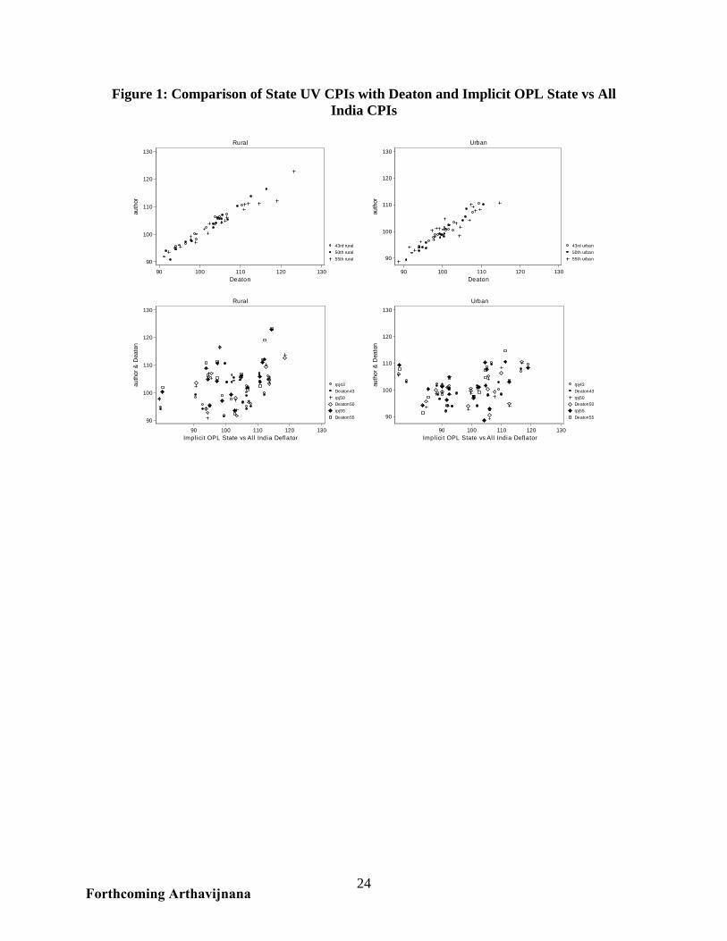
24

Figure 1: Comparison of State UV CPIs with Deaton and Implicit OPL State vs All India CPIs

90

100

110

120

130

auth

or

90 100 110 120 130Deaton

43rd rural50th rural55th rural

Rural

90

100

110

120

130

auth

or

90 100 110 120 130Deaton

43rd urban50th urban55th urban

Urban

90

100

110

120

130

auth

or &

Dea

ton

90 100 110 120 130Impl ici t OPL State vs Al l India Deflator

rpj43Deaton43rpj50Deaton50rpj55Deaton55

Rural

90

100

110

120

130

auth

or &

Dea

ton

90 100 110 120 130Impl ici t OPL State vs Al l India Deflator

rpj43Deaton43rpj50Deaton50rpj55Deaton55

Urban


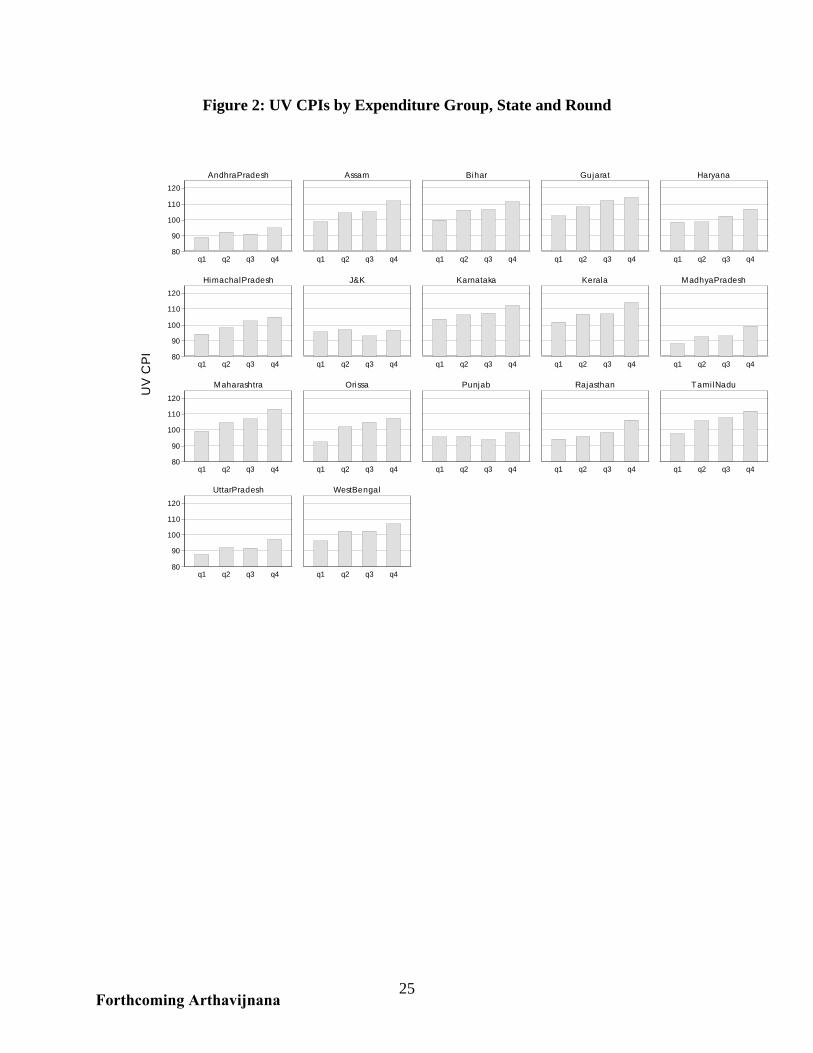
25

Figure 2: UV CPIs by Expenditure Group, State and Round

80

90

100

110

120

80

90

100

110

120

80

90

100

110

120

80

90

100

110

120

q1 q2 q3 q4 q1 q2 q3 q4 q1 q2 q3 q4 q1 q2 q3 q4 q1 q2 q3 q4



q1 q2 q3 q4 q1 q2 q3 q4

AndhraPradesh Assam Bihar Gujarat Haryana

HimachalPradesh J&K Karnataka Kerala MadhyaPradesh

Maharashtra Orissa Punjab Rajasthan TamilNadu

UttarPradesh WestBengal

UV

CP

I


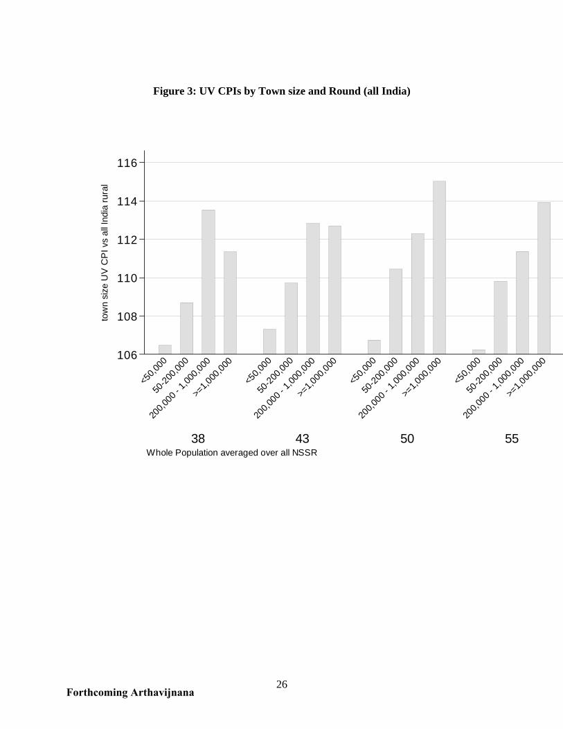
26

Figure 3: UV CPIs by Town size and Round (all India)

106

108

110

112

114

116

tow

n si

ze U

V C

PI v

s al

l Ind

ia ru

ral

38 43 50 55

<50,0

00

50-20

0,000

200,0

00 - 1

,000,0

00

>=1,0

00,00

0

<50,0

00

50-20

0,000

200,0

00 - 1

,000,0

00

>=1,0

00,00

0

<50,0

00

50-20

0,000

200,0

00 - 1

,000,0

00

>=1,0

00,00

0

<50,0

00

50-20

0,000

200,0

00 - 1

,000,0

00

>=1,0

00,00

0

Whole Population averaged over all NSSR


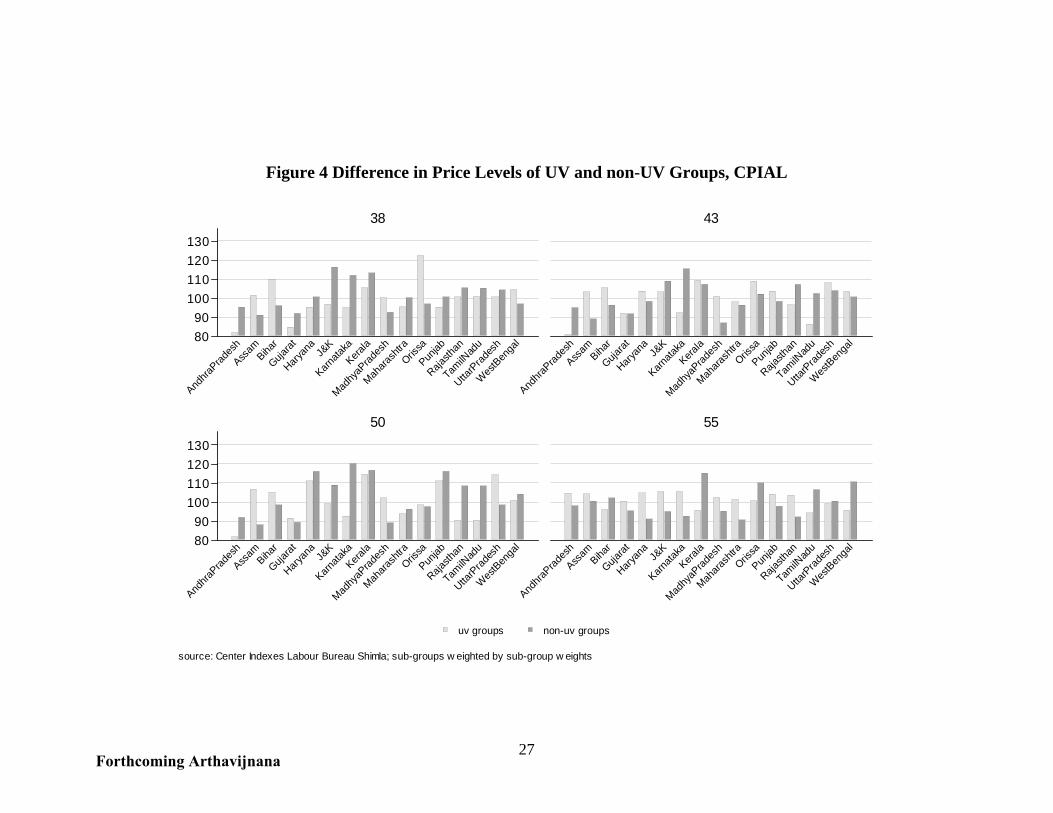
27

Figure 4 Difference in Price Levels of UV and non-UV Groups, CPIAL

8090

100110120130

8090

100110120130

Andhra

Prades

hAss

amBiha

rGuja

ratHary

ana

J&K

Karnata

kaKera

la

Madhy

aPrad

esh

Mahara

shtra

Orissa

Punjab

Rajasth

anTam

ilNad

u

UttarP

rades

hW

estB

enga

lAnd

hraPrad

esh

Assam

Bihar

Gujarat

Haryan

aJ&

KKarn

ataka

Kerala

Madhy

aPrad

esh

Mahara

shtra

Orissa

Punjab

Rajasth

anTam

ilNad

u

UttarP

rades

hW

estB

enga

l

Andhra

Prades

hAss

amBiha

rGuja

ratHary

ana

J&K

Karnata

kaKera

la

Madhy

aPrad

esh

Mahara

shtra

Orissa

Punjab

Rajasth

anTam

ilNad

u

UttarP

rades

hW

estB

enga

lAnd

hraPrad

esh

Assam

Bihar

Gujarat

Haryan

aJ&

KKarn

ataka

Kerala

Madhy

aPrad

esh

Mahara

shtra

Orissa

Punjab

Rajasth

anTam

ilNad

u

UttarP

rades

hW

estB

enga

l

38 43

50 55

uv groups non-uv groups

source: Center Indexes Labour Bureau Shimla; sub-groups w eighted by sub-group w eights


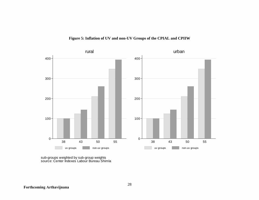
28

Figure 5: Inflation of UV and non-UV Groups of the CPIAL and CPIIW

0

100

200

300

400

38 43 50 55

rural


0

100

200

300

400

38 43 50 55

urban


sub-groups weighted by sub-group weightssource: Center Indexes Labour Bureau Shimla


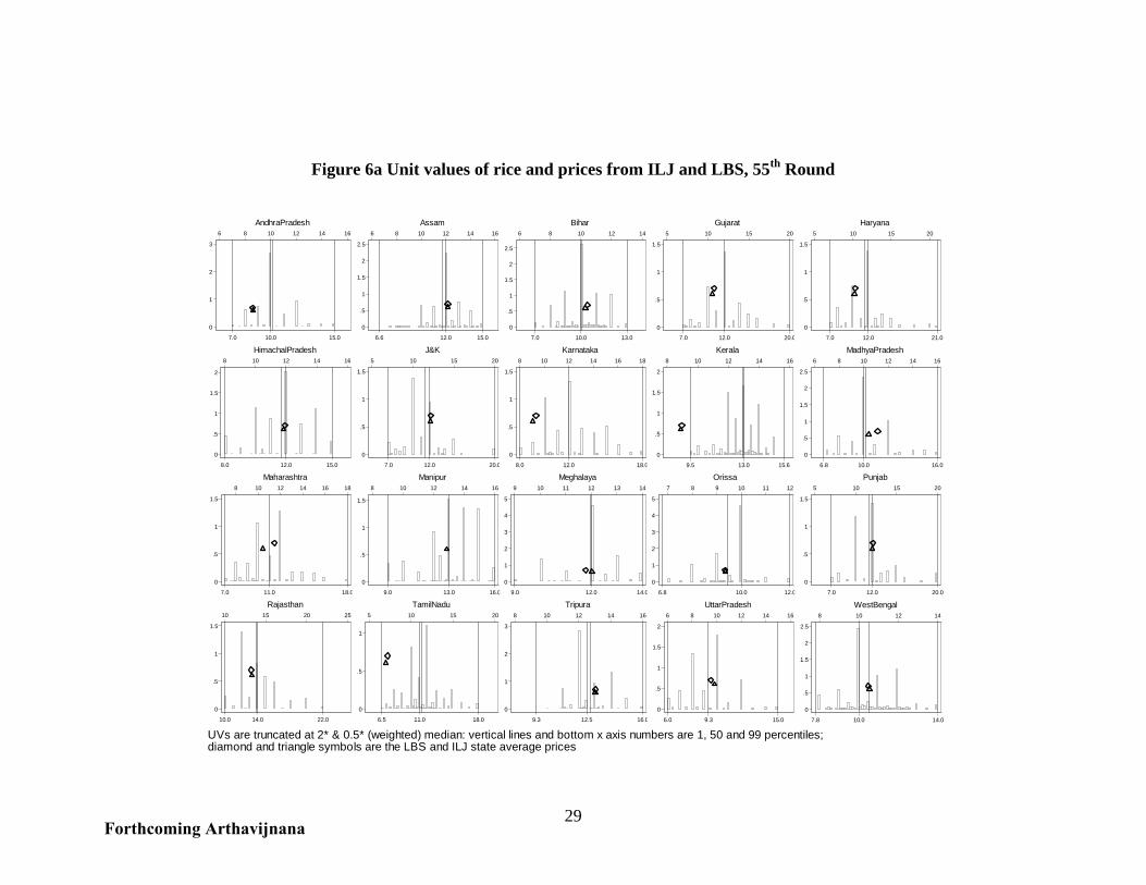
29

Figure 6a Unit values of rice and prices from ILJ and LBS, 55th Round

0

1

2

3

6 8 10 12 14 16

7.0 10.0 15.0

AndhraPradesh

0

.5

1

1.5

2

2.5

6 8 10 12 14 16

6.6 12.0 15.0

Assam

0

.5

1

1.5

2

2.5

6 8 10 12 14

7.0 10.0 13.0

Bihar

0

.5

1

1.5

5 10 15 20

7.0 12.0 20.0

Gujarat

0

.5

1

1.5

5 10 15 20

7.0 12.0 21.0

Haryana

0

.5

1

1.5

2

8 10 12 14 16

8.0 12.0 15.0

HimachalPradesh

0

.5

1

1.5

5 10 15 20

7.0 12.0 20.0

J&K

0

.5

1

1.5

8 10 12 14 16 18

8.0 12.0 18.0

Karnataka

0

.5

1

1.5

2

8 10 12 14 16

9.5 13.0 15.6

Kerala

0

.5

1

1.5

2

2.5

6 8 10 12 14 16

6.8 10.0 16.0

MadhyaPradesh

0

.5

1

1.5

8 10 12 14 16 18

7.0 11.0 18.0

Maharashtra

0

.5

1

1.5

8 10 12 14 16

9.0 13.0 16.0

Manipur

0

1

2

3

4

5

9 10 11 12 13 14

9.0 12.0 14.0

Meghalaya

0

1

2

3

4

5

7 8 9 10 11 12

6.8 10.0 12.0

Orissa

0

.5

1

1.5

5 10 15 20

7.0 12.0 20.0

Punjab

0

.5

1

1.5

10 15 20 25

10.0 14.0 22.0

Rajasthan

0

.5

1

5 10 15 20

6.5 11.0 18.0

TamilNadu

0

1

2

3

8 10 12 14 16

9.3 12.5 16.0

Tripura

0

.5

1

1.5

2

6 8 10 12 14 16

6.0 9.3 15.0

UttarPradesh

0

.5

1

1.5

2

2.5

8 10 12 14

7.8 10.0 14.0

WestBengal

UVs are truncated at 2* & 0.5* (weighted) median: vertical lines and bottom x axis numbers are 1, 50 and 99 percentiles;diamond and triangle symbols are the LBS and ILJ state average prices


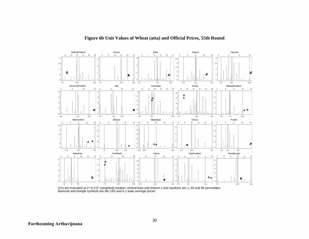
30

Figure 6b Unit Values of Wheat (atta) and Official Prices, 55th Round

0

.5

1

1.5

2

8 10 12 14 16 18

7.0 12.0 18.0

AndhraPradesh

0

1

2

3

8 9 10 11 12 13

7.6 11.0 13.0

Assam

0

1

2

3

6 7 8 9 10 11

5.5 8.5 10.7

Bihar

0

.5

1

1.5

2

2.5

4 6 8 10 12

5.0 8.0 12.0

Gujarat

0

.5

1

1.5

2

4 6 8 10

4.5 6.5 10.0

Haryana

0

1

2

3

4

6 8 10 12

6.0 9.0 11.0

HimachalPradesh

0

1

2

3

4

6 8 10 12

6.0 8.5 10.0

J&K

0

.2

.4

.6

.8

1

6 8 10 12 14 16

5.0 9.0 16.0

Karnataka

0

.2

.4

.6

.8

8 10 12 14 16 18

7.2 13.0 18.0

Kerala

0

1

2

3

4

4 6 8 10 12

5.0 7.0 10.0

MadhyaPradesh

0

.5

1

1.5

2

2.5

4 6 8 10 12

5.0 8.0 12.0

Maharashtra

0

2

4

6

8

6 8 10 12 14

7.0 10.0 12.0

Manipur

0

1

2

3

4

5

10 11 12 13 14

10.0 10.6 14.0

Meghalaya

0

2

4

6

8 9 10 11 12 13

8.5 10.0 13.0

Orissa

0

1

2

3

4

4 6 8 10 12

5.0 6.5 9.0

Punjab

0

1

2

3

4

4 6 8 10 12 14

5.0 7.0 9.0

Rajasthan

0

.2

.4

.6

.8

5 10 15 20

7.0 13.0 20.0

TamilNadu

0

2

4

6

8

10

11 12 13 14

10.3 12.0 14.0

Tripura

0

1

2

3

4

5 6 7 8 9 10

5.0 6.5 9.0

UttarPradesh

0

1

2

3

4

5

7 8 9 10 11 12

7.0 10.0 12.0

WestBengal

UVs are truncated at 2* & 0.5* (weighted) median: vertical lines and bottom x axis numbers are 1, 50 and 99 percentiles;diamond and triangle symbols are the LBS and ILJ state average prices


31

Figure 7: Average Budget Shares by Town Size and Round (all India)

45

50

55

60

65

UV

AV

BS

vs

all I

ndia

Rur

al

38 43 50 55

<50,0

0050

-200,0

00

200,0

00 - 1

,000,0

00>=

1,000

,000

<50,0

0050

-200,0

00

200,0

00 - 1

,000,0

00>=

1,000

,000

<50,0

0050

-200,0

00

200,0

00 - 1

,000,0

00>=

1,000

,000

<50,0

0050

-200,0

00

200,0

00 - 1

,000,0

00>=

1,000

,000

UV AVBSs by Townsize, and Roundwhole population


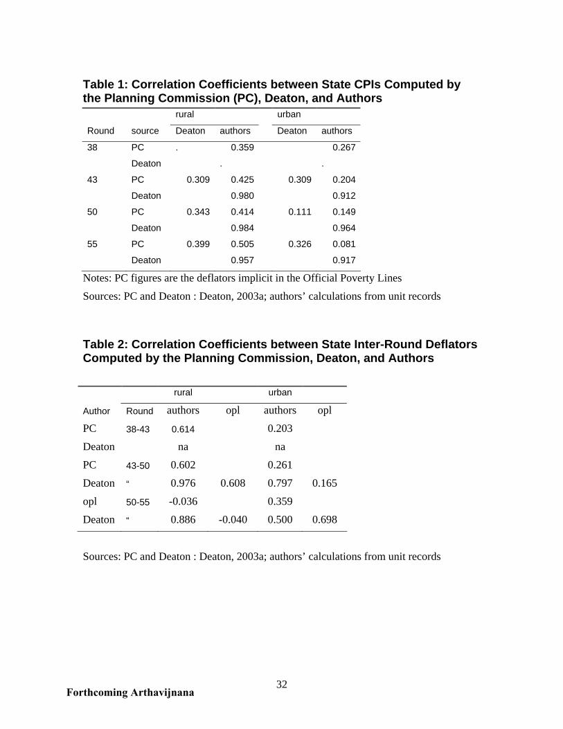
32

Table 1: Correlation Coefficients between State CPIs Computed by the Planning Commission (PC), Deaton, and Authors rural urban

Round source Deaton authors Deaton authors

38 PC . 0.359 0.267

Deaton . .

43 PC 0.309 0.425 0.309 0.204

Deaton 0.980 0.912

50 PC 0.343 0.414 0.111 0.149

Deaton 0.984 0.964

55 PC 0.399 0.505 0.326 0.081

Deaton 0.957 0.917

Notes: PC figures are the deflators implicit in the Official Poverty Lines

Sources: PC and Deaton : Deaton, 2003a; authors’ calculations from unit records

Table 2: Correlation Coefficients between State Inter-Round Deflators Computed by the Planning Commission, Deaton, and Authors rural urban

Author Round authors opl authors opl

PC 38-43 0.614 0.203

Deaton na na

PC 43-50 0.602 0.261

Deaton “ 0.976 0.608 0.797 0.165

opl 50-55 -0.036 0.359

Deaton “ 0.886 -0.040 0.500 0.698



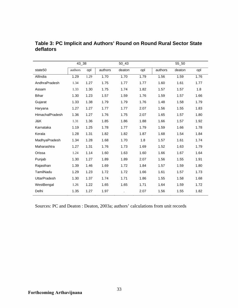
33

Table 3: PC Implicit and Authors’ Round on Round Rural Sector State deflators 43_38 50_43 55_50

state50 authors opl authors deaton opl authors deaton opl

AllIndia 1.29 1.29 1.70 1.70 1.79 1.56 1.59 1.76

AndhraPradesh 1.34 1.27 1.75 1.77 1.77 1.60 1.61 1.77

Assam 1.33 1.30 1.75 1.74 1.82 1.57 1.57 1.8

Bihar 1.30 1.23 1.57 1.59 1.76 1.59 1.57 1.66

Gujarat 1.33 1.38 1.79 1.79 1.76 1.48 1.58 1.79

Haryana 1.27 1.27 1.77 1.77 2.07 1.56 1.55 1.83

HimachalPradesh 1.36 1.27 1.76 1.75 2.07 1.65 1.57 1.80

J&K 1.31 1.36 1.85 1.86 1.88 1.66 1.57 1.92

Karnataka 1.19 1.25 1.78 1.77 1.79 1.59 1.66 1.78

Kerala 1.28 1.31 1.82 1.82 1.87 1.68 1.54 1.84

MadhyaPradesh 1.34 1.28 1.68 1.70 1.8 1.57 1.61 1.74

Maharashtra 1.27 1.31 1.76 1.73 1.69 1.52 1.63 1.79

Orissa 1.24 1.14 1.60 1.63 1.60 1.66 1.67 1.64

Punjab 1.30 1.27 1.89 1.89 2.07 1.56 1.55 1.91

Rajasthan 1.39 1.46 1.69 1.72 1.84 1.57 1.59 1.80

TamilNadu 1.29 1.23 1.72 1.72 1.66 1.61 1.57 1.73

UttarPradesh 1.30 1.37 1.74 1.71 1.86 1.55 1.58 1.68

WestBengal 1.26 1.22 1.65 1.65 1.71 1.64 1.59 1.72

Delhi 1.35 1.27 1.97 . 2.07 1.56 1.55 1.82



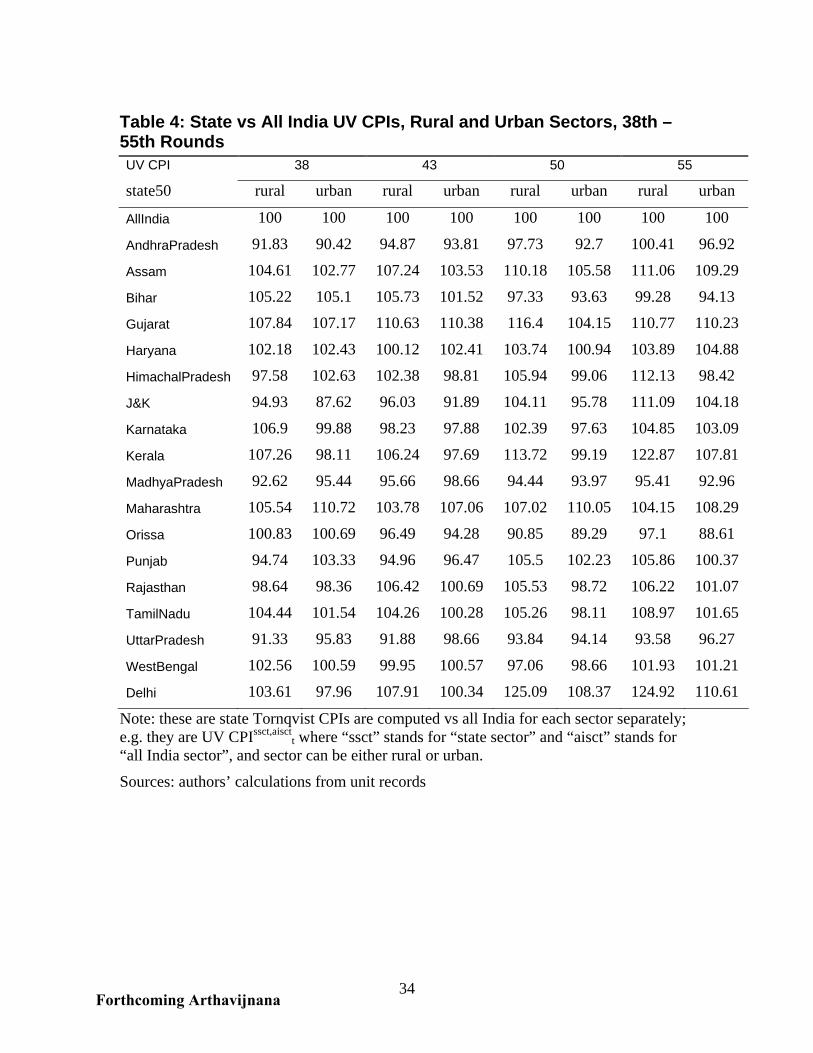
34

Table 4: State vs All India UV CPIs, Rural and Urban Sectors, 38th – 55th Rounds UV CPI 38 43 50 55

state50 rural urban rural urban rural urban rural urban

AllIndia 100 100 100 100 100 100 100 100

AndhraPradesh 91.83 90.42 94.87 93.81 97.73 92.7 100.41 96.92

Assam 104.61 102.77 107.24 103.53 110.18 105.58 111.06 109.29

Bihar 105.22 105.1 105.73 101.52 97.33 93.63 99.28 94.13

Gujarat 107.84 107.17 110.63 110.38 116.4 104.15 110.77 110.23

Haryana 102.18 102.43 100.12 102.41 103.74 100.94 103.89 104.88

HimachalPradesh 97.58 102.63 102.38 98.81 105.94 99.06 112.13 98.42

J&K 94.93 87.62 96.03 91.89 104.11 95.78 111.09 104.18

Karnataka 106.9 99.88 98.23 97.88 102.39 97.63 104.85 103.09

Kerala 107.26 98.11 106.24 97.69 113.72 99.19 122.87 107.81

MadhyaPradesh 92.62 95.44 95.66 98.66 94.44 93.97 95.41 92.96

Maharashtra 105.54 110.72 103.78 107.06 107.02 110.05 104.15 108.29

Orissa 100.83 100.69 96.49 94.28 90.85 89.29 97.1 88.61

Punjab 94.74 103.33 94.96 96.47 105.5 102.23 105.86 100.37

Rajasthan 98.64 98.36 106.42 100.69 105.53 98.72 106.22 101.07

TamilNadu 104.44 101.54 104.26 100.28 105.26 98.11 108.97 101.65

UttarPradesh 91.33 95.83 91.88 98.66 93.84 94.14 93.58 96.27

WestBengal 102.56 100.59 99.95 100.57 97.06 98.66 101.93 101.21

Delhi 103.61 97.96 107.91 100.34 125.09 108.37 124.92 110.61

Note: these are state Tornqvist CPIs are computed vs all India for each sector separately; e.g. they are UV CPIssct,aisct

t where “ssct” stands for “state sector” and “aisct” stands for “all India sector”, and sector can be either rural or urban.

Sources: authors’ calculations from unit records


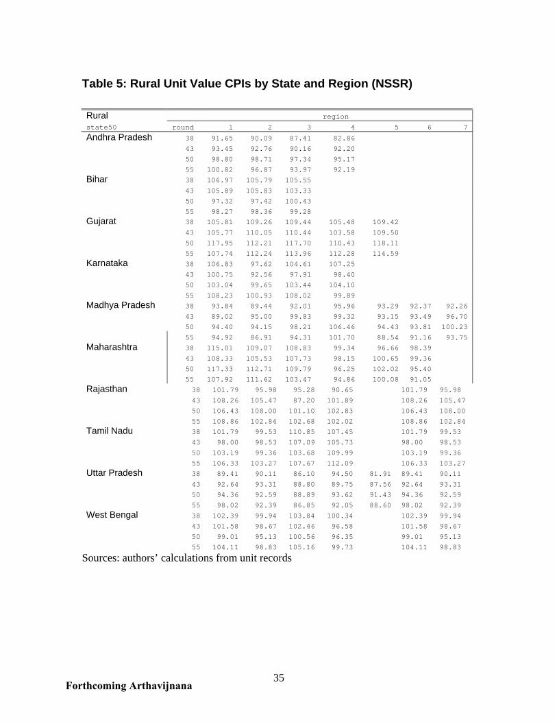
35

Table 5: Rural Unit Value CPIs by State and Region (NSSR)

Rural region

state50 round 1 2 3 4 5 6 7

Andhra Pradesh 38 91.65 90.09 87.41 82.86 43 93.45 92.76 90.16 92.20 50 98.80 98.71 97.34 95.17 55 100.82 96.87 93.97 92.19 Bihar 38 106.97 105.79 105.55 43 105.89 105.83 103.33 50 97.32 97.42 100.43 55 98.27 98.36 99.28 Gujarat 38 105.81 109.26 109.44 105.48 109.42 43 105.77 110.05 110.44 103.58 109.50 50 117.95 112.21 117.70 110.43 118.11 55 107.74 112.24 113.96 112.28 114.59 Karnataka 38 106.83 97.62 104.61 107.25 43 100.75 92.56 97.91 98.40 50 103.04 99.65 103.44 104.10 55 108.23 100.93 108.02 99.89 Madhya Pradesh 38 93.84 89.44 92.01 95.96 93.29 92.37 92.26 43 89.02 95.00 99.83 99.32 93.15 93.49 96.70 50 94.40 94.15 98.21 106.46 94.43 93.81 100.23 55 94.92 86.91 94.31 101.70 88.54 91.16 93.75 Maharashtra 38 115.01 109.07 108.83 99.34 96.66 98.39 43 108.33 105.53 107.73 98.15 100.65 99.36 50 117.33 112.71 109.79 96.25 102.02 95.40 55 107.92 111.62 103.47 94.86 100.08 91.05 Rajasthan 38 101.79 95.98 95.28 90.65 101.79 95.98 43 108.26 105.47 87.20 101.89 108.26 105.47 50 106.43 108.00 101.10 102.83 106.43 108.00 55 108.86 102.84 102.68 102.02 108.86 102.84 Tamil Nadu 38 101.79 99.53 110.85 107.45 101.79 99.53 43 98.00 98.53 107.09 105.73 98.00 98.53 50 103.19 99.36 103.68 109.99 103.19 99.36 55 106.33 103.27 107.67 112.09 106.33 103.27 Uttar Pradesh 38 89.41 90.11 86.10 94.50 81.91 89.41 90.11 43 92.64 93.31 88.80 89.75 87.56 92.64 93.31 50 94.36 92.59 88.89 93.62 91.43 94.36 92.59 55 98.02 92.39 86.85 92.05 88.60 98.02 92.39 West Bengal 38 102.39 99.94 103.84 100.34 102.39 99.94 43 101.58 98.67 102.46 96.58 101.58 98.67 50 99.01 95.13 100.56 96.35 99.01 95.13 55 104.11 98.83 105.16 99.73 104.11 98.83

Sources: authors’ calculations from unit records


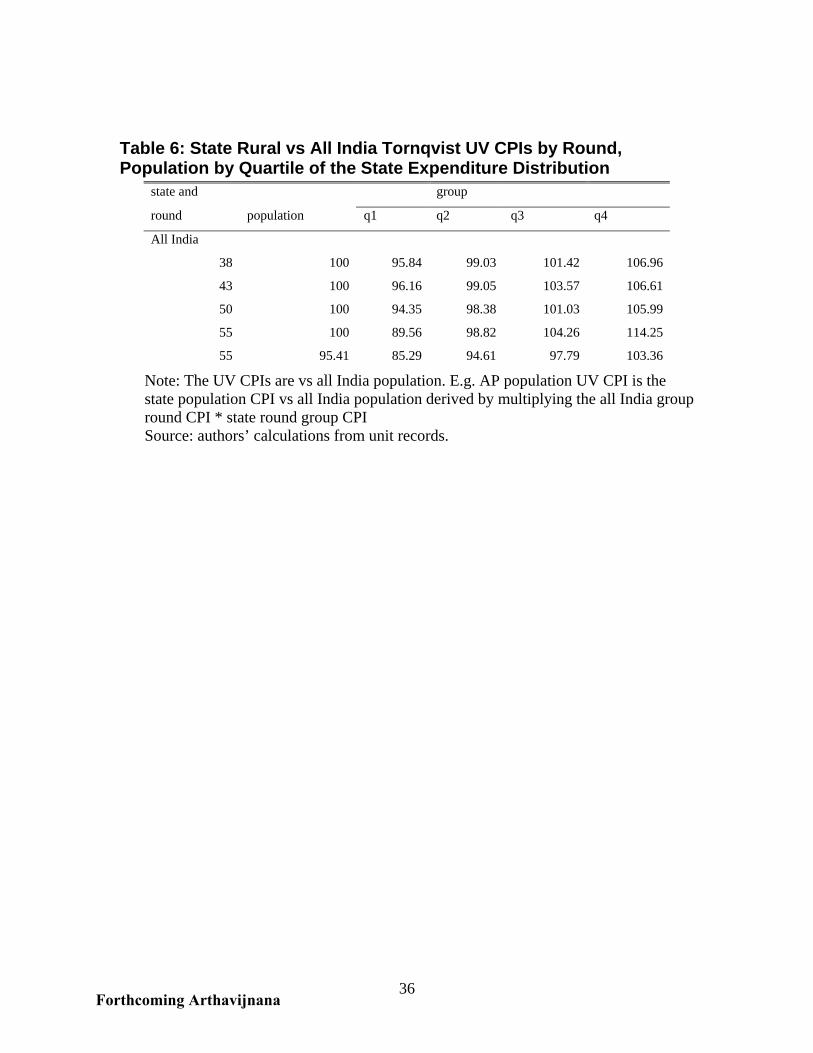
36

Table 6: State Rural vs All India Tornqvist UV CPIs by Round, Population by Quartile of the State Expenditure Distribution

state and group

round population q1 q2 q3 q4

All India

38 100 95.84 99.03 101.42 106.96

43 100 96.16 99.05 103.57 106.61

50 100 94.35 98.38 101.03 105.99

55 100 89.56 98.82 104.26 114.25

55 95.41 85.29 94.61 97.79 103.36

Note: The UV CPIs are vs all India population. E.g. AP population UV CPI is the state population CPI vs all India population derived by multiplying the all India group round CPI * state round group CPI Source: authors’ calculations from unit records.


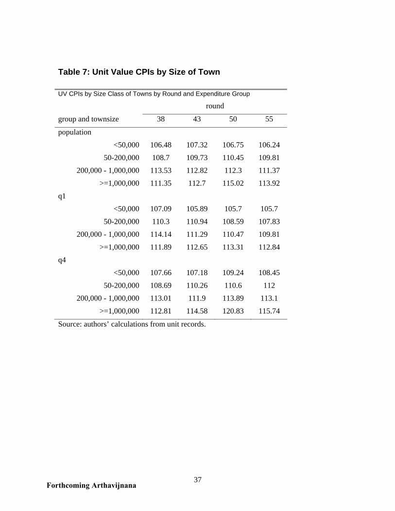
37

Table 7: Unit Value CPIs by Size of Town

Source: authors’ calculations from unit records.

UV CPIs by Size Class of Towns by Round and Expenditure Group

round

group and townsize 38 43 50 55

population

<50,000 106.48 107.32 106.75 106.24

50-200,000 108.7 109.73 110.45 109.81

200,000 - 1,000,000 113.53 112.82 112.3 111.37

>=1,000,000 111.35 112.7 115.02 113.92

q1

<50,000 107.09 105.89 105.7 105.7

50-200,000 110.3 110.94 108.59 107.83

200,000 - 1,000,000 114.14 111.29 110.47 109.81

>=1,000,000 111.89 112.65 113.31 112.84

q4

<50,000 107.66 107.18 109.24 108.45

50-200,000 108.69 110.26 110.6 112

200,000 - 1,000,000 113.01 111.9 113.89 113.1

>=1,000,000 112.81 114.58 120.83 115.74


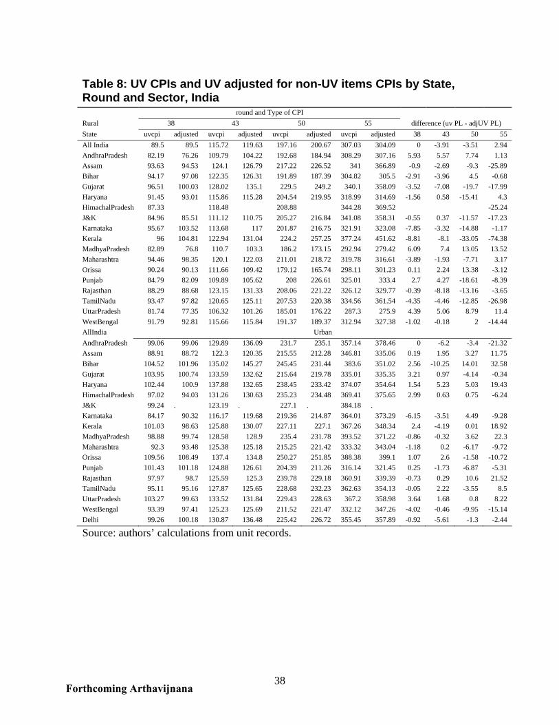
38

Table 8: UV CPIs and UV adjusted for non-UV items CPIs by State, Round and Sector, India round and Type of CPI Rural 38 43 50 55 difference (uv PL - adjUV PL) State uvcpi adjusted uvcpi adjusted uvcpi adjusted uvcpi adjusted 38 43 50 55 All India 89.5 89.5 115.72 119.63 197.16 200.67 307.03 304.09 0 -3.91 -3.51 2.94 AndhraPradesh 82.19 76.26 109.79 104.22 192.68 184.94 308.29 307.16 5.93 5.57 7.74 1.13 Assam 93.63 94.53 124.1 126.79 217.22 226.52 341 366.89 -0.9 -2.69 -9.3 -25.89 Bihar 94.17 97.08 122.35 126.31 191.89 187.39 304.82 305.5 -2.91 -3.96 4.5 -0.68 Gujarat 96.51 100.03 128.02 135.1 229.5 249.2 340.1 358.09 -3.52 -7.08 -19.7 -17.99 Haryana 91.45 93.01 115.86 115.28 204.54 219.95 318.99 314.69 -1.56 0.58 -15.41 4.3 HimachalPradesh 87.33 118.48 208.88 344.28 369.52 -25.24 J&K 84.96 85.51 111.12 110.75 205.27 216.84 341.08 358.31 -0.55 0.37 -11.57 -17.23 Karnataka 95.67 103.52 113.68 117 201.87 216.75 321.91 323.08 -7.85 -3.32 -14.88 -1.17 Kerala 96 104.81 122.94 131.04 224.2 257.25 377.24 451.62 -8.81 -8.1 -33.05 -74.38 MadhyaPradesh 82.89 76.8 110.7 103.3 186.2 173.15 292.94 279.42 6.09 7.4 13.05 13.52 Maharashtra 94.46 98.35 120.1 122.03 211.01 218.72 319.78 316.61 -3.89 -1.93 -7.71 3.17 Orissa 90.24 90.13 111.66 109.42 179.12 165.74 298.11 301.23 0.11 2.24 13.38 -3.12 Punjab 84.79 82.09 109.89 105.62 208 226.61 325.01 333.4 2.7 4.27 -18.61 -8.39 Rajasthan 88.29 88.68 123.15 131.33 208.06 221.22 326.12 329.77 -0.39 -8.18 -13.16 -3.65 TamilNadu 93.47 97.82 120.65 125.11 207.53 220.38 334.56 361.54 -4.35 -4.46 -12.85 -26.98 UttarPradesh 81.74 77.35 106.32 101.26 185.01 176.22 287.3 275.9 4.39 5.06 8.79 11.4 WestBengal 91.79 92.81 115.66 115.84 191.37 189.37 312.94 327.38 -1.02 -0.18 2 -14.44 AllIndia Urban AndhraPradesh 99.06 99.06 129.89 136.09 231.7 235.1 357.14 378.46 0 -6.2 -3.4 -21.32 Assam 88.91 88.72 122.3 120.35 215.55 212.28 346.81 335.06 0.19 1.95 3.27 11.75 Bihar 104.52 101.96 135.02 145.27 245.45 231.44 383.6 351.02 2.56 -10.25 14.01 32.58 Gujarat 103.95 100.74 133.59 132.62 215.64 219.78 335.01 335.35 3.21 0.97 -4.14 -0.34 Haryana 102.44 100.9 137.88 132.65 238.45 233.42 374.07 354.64 1.54 5.23 5.03 19.43 HimachalPradesh 97.02 94.03 131.26 130.63 235.23 234.48 369.41 375.65 2.99 0.63 0.75 -6.24 J&K 99.24 . 123.19 . 227.1 . 384.18 . Karnataka 84.17 90.32 116.17 119.68 219.36 214.87 364.01 373.29 -6.15 -3.51 4.49 -9.28 Kerala 101.03 98.63 125.88 130.07 227.11 227.1 367.26 348.34 2.4 -4.19 0.01 18.92 MadhyaPradesh 98.88 99.74 128.58 128.9 235.4 231.78 393.52 371.22 -0.86 -0.32 3.62 22.3 Maharashtra 92.3 93.48 125.38 125.18 215.25 221.42 333.32 343.04 -1.18 0.2 -6.17 -9.72 Orissa 109.56 108.49 137.4 134.8 250.27 251.85 388.38 399.1 1.07 2.6 -1.58 -10.72 Punjab 101.43 101.18 124.88 126.61 204.39 211.26 316.14 321.45 0.25 -1.73 -6.87 -5.31 Rajasthan 97.97 98.7 125.59 125.3 239.78 229.18 360.91 339.39 -0.73 0.29 10.6 21.52 TamilNadu 95.11 95.16 127.87 125.65 228.68 232.23 362.63 354.13 -0.05 2.22 -3.55 8.5 UttarPradesh 103.27 99.63 133.52 131.84 229.43 228.63 367.2 358.98 3.64 1.68 0.8 8.22 WestBengal 93.39 97.41 125.23 125.69 211.52 221.47 332.12 347.26 -4.02 -0.46 -9.95 -15.14 Delhi 99.26 100.18 130.87 136.48 225.42 226.72 355.45 357.89 -0.92 -5.61 -1.3 -2.44



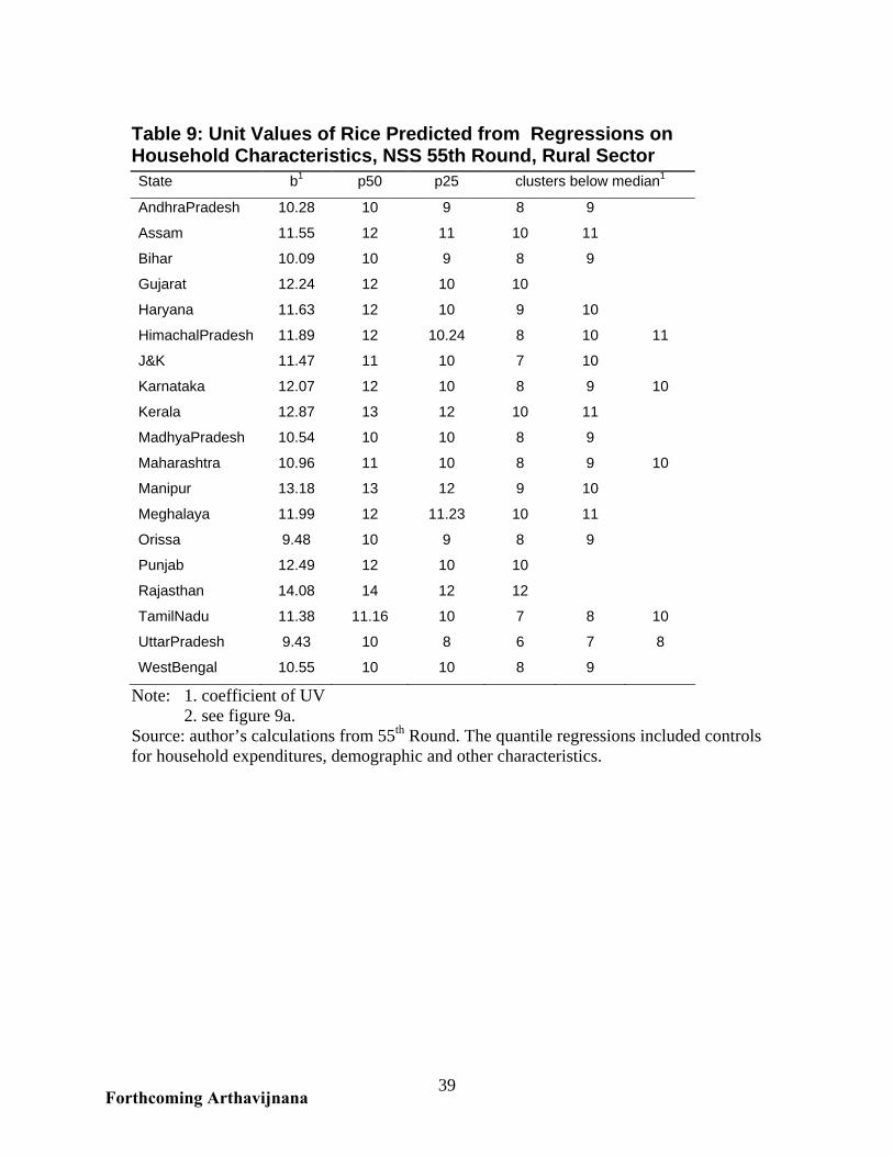
39

Table 9: Unit Values of Rice Predicted from Regressions on Household Characteristics, NSS 55th Round, Rural Sector State b1 p50 p25 clusters below median1

AndhraPradesh 10.28 10 9 8 9

Assam 11.55 12 11 10 11

Bihar 10.09 10 9 8 9

Gujarat 12.24 12 10 10

Haryana 11.63 12 10 9 10

HimachalPradesh 11.89 12 10.24 8 10 11

J&K 11.47 11 10 7 10

Karnataka 12.07 12 10 8 9 10

Kerala 12.87 13 12 10 11

MadhyaPradesh 10.54 10 10 8 9

Maharashtra 10.96 11 10 8 9 10

Manipur 13.18 13 12 9 10

Meghalaya 11.99 12 11.23 10 11

Orissa 9.48 10 9 8 9

Punjab 12.49 12 10 10

Rajasthan 14.08 14 12 12

TamilNadu 11.38 11.16 10 7 8 10

UttarPradesh 9.43 10 8 6 7 8

WestBengal 10.55 10 10 8 9

Note: 1. coefficient of UV 2. see figure 9a. Source: author’s calculations from 55th Round. The quantile regressions included controls for household expenditures, demographic and other characteristics.


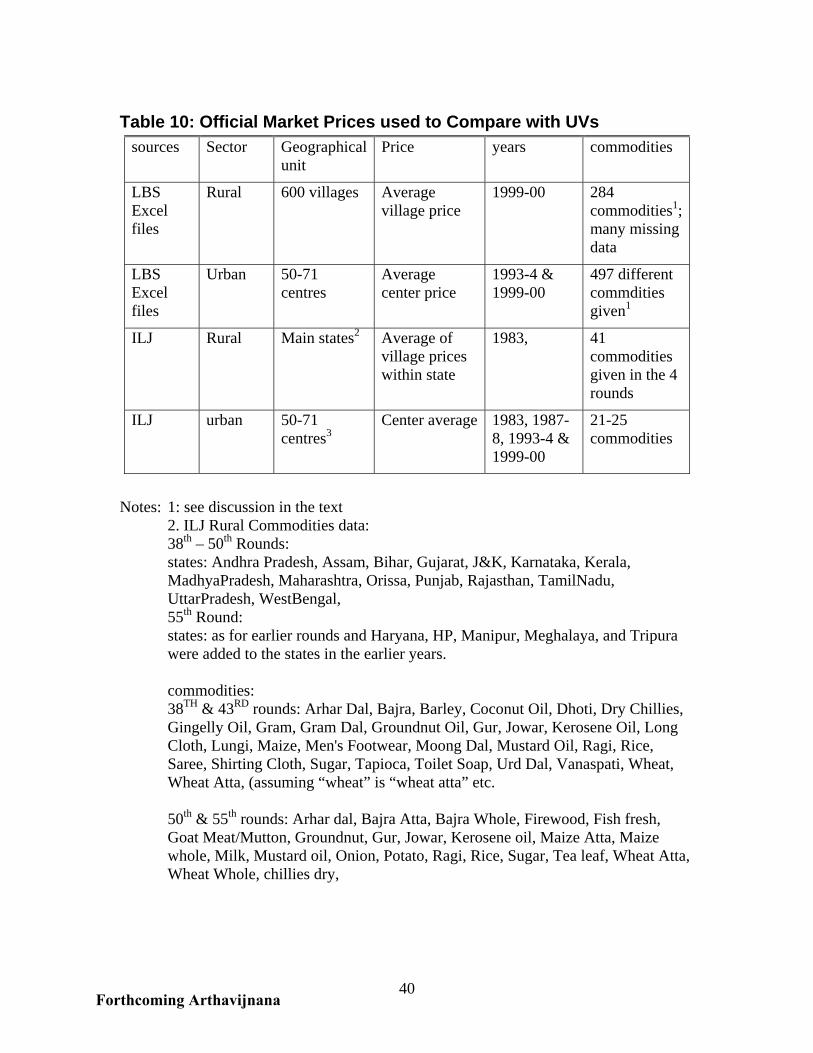
40

Table 10: Official Market Prices used to Compare with UVs sources Sector Geographical

unit Price years commodities

LBS Excel files

Rural 600 villages Average village price

1999-00 284 commodities1; many missing data

LBS Excel files

Urban 50-71 centres

Average center price

1993-4 & 1999-00

497 different commdities given1

ILJ Rural Main states2 Average of village prices within state

1983, 41 commodities given in the 4 rounds

ILJ urban 50-71 centres3

Center average 1983, 1987-8, 1993-4 & 1999-00

21-25 commodities

Notes: 1: see discussion in the text 2. ILJ Rural Commodities data: 38th – 50th Rounds: states: Andhra Pradesh, Assam, Bihar, Gujarat, J&K, Karnataka, Kerala, MadhyaPradesh, Maharashtra, Orissa, Punjab, Rajasthan, TamilNadu, UttarPradesh, WestBengal, 55th Round: states: as for earlier rounds and Haryana, HP, Manipur, Meghalaya, and Tripura were added to the states in the earlier years. commodities: 38TH & 43RD rounds: Arhar Dal, Bajra, Barley, Coconut Oil, Dhoti, Dry Chillies, Gingelly Oil, Gram, Gram Dal, Groundnut Oil, Gur, Jowar, Kerosene Oil, Long Cloth, Lungi, Maize, Men's Footwear, Moong Dal, Mustard Oil, Ragi, Rice, Saree, Shirting Cloth, Sugar, Tapioca, Toilet Soap, Urd Dal, Vanaspati, Wheat, Wheat Atta, (assuming “wheat” is “wheat atta” etc. 50th & 55th rounds: Arhar dal, Bajra Atta, Bajra Whole, Firewood, Fish fresh, Goat Meat/Mutton, Groundnut, Gur, Jowar, Kerosene oil, Maize Atta, Maize whole, Milk, Mustard oil, Onion, Potato, Ragi, Rice, Sugar, Tea leaf, Wheat Atta, Wheat Whole, chillies dry,


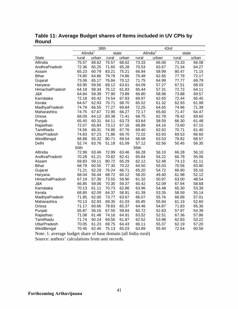
41

Table 11: Average Budget shares of Items included in UV CPIs by Round 38th 43rd AlIndia1 state AlIndia1 state State rural urban rural urban rural urban rural urban AllIndia 75.57 68.62 75.57 68.62 73.33 66.08 73.33 66.08AndhraPradesh 72.36 65.25 71.65 65.28 70.53 63.67 71.34 64.27Assam 65.23 60.79 83.21 75.21 66.94 58.99 80.47 71.15Bihar 74.80 64.86 79.78 74.86 70.48 62.65 77.78 72.17Gujarat 73.06 65.17 76.84 70.12 71.75 64.99 77.77 69.79Haryana 63.90 59.56 69.12 63.61 64.09 57.27 67.51 68.03HimachalPradesh 64.18 58.34 75.12 61.83 65.44 57.31 72.72 64.11J&K 64.84 59.39 77.90 73.89 66.80 58.98 73.88 69.57Karnataka 72.18 65.42 74.54 67.83 69.97 62.65 72.44 65.45Kerala 64.67 62.93 70.71 68.70 65.52 61.32 62.93 61.99MadhyaPradesh 74.79 66.55 77.27 69.84 72.25 64.65 74.96 71.39Maharashtra 74.75 67.67 72.95 66.27 72.17 65.60 71.47 64.47Orissa 68.09 64.12 83.38 71.41 68.75 62.78 78.42 69.60Punjab 65.40 60.31 64.11 63.73 63.64 58.59 66.30 61.48Rajasthan 72.07 65.84 73.12 67.16 68.89 64.16 73.60 67.15TamilNadu 74.56 66.31 74.85 67.76 69.40 62.62 70.71 61.40UttarPradesh 74.83 67.23 71.86 69.70 72.02 63.93 69.53 66.60WestBengal 68.88 65.32 80.71 69.54 68.08 63.53 78.82 68.57Delhi 52.74 63.76 51.18 61.09 57.12 62.56 50.45 56.35 50th 55th AllIndia 72.99 63.46 72.99 63.46 66.28 56.10 66.28 56.10AndhraPradesh 70.28 61.21 70.82 62.41 65.84 54.22 66.78 55.06Assam 69.83 59.11 80.72 65.29 62.12 52.48 74.13 61.11Bihar 68.79 60.55 77.30 70.22 64.50 55.03 70.56 63.90Gujarat 71.21 62.29 76.24 66.71 65.20 54.72 66.90 55.16Haryana 68.04 56.44 68.72 60.12 58.20 49.40 61.98 52.12HimachalPradesh 67.19 57.39 73.55 59.90 61.32 50.97 63.00 48.54J&K 66.85 59.06 70.30 59.37 60.42 52.09 67.94 58.68Karnataka 70.13 61.11 70.73 62.86 63.96 54.48 65.30 53.39Kerala 68.85 62.09 64.37 58.91 61.39 53.35 58.59 55.14MadhyaPradesh 71.85 62.00 73.77 63.67 66.07 55.76 66.89 57.01Maharashtra 70.13 62.93 69.35 61.03 65.85 55.94 61.19 52.60Orissa 71.17 60.66 78.83 65.37 64.46 54.87 71.83 65.36Punjab 65.87 56.16 67.55 59.84 60.72 52.83 57.97 54.39Rajasthan 71.08 61.48 74.16 64.91 63.52 52.51 67.36 57.86TamilNadu 71.74 60.24 69.56 61.87 62.52 53.98 62.83 53.22UttarPradesh 70.05 61.23 69.75 64.43 66.11 55.37 62.19 57.20WestBengal 70.45 62.46 75.13 65.03 63.89 55.40 72.54 60.56Note: 1. average budget share of base domain (all India rural) Source: authors’ calculations from unit records.


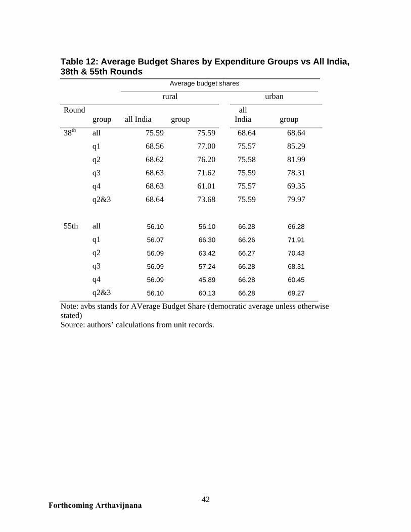
42

Table 12: Average Budget Shares by Expenditure Groups vs All India, 38th & 55th Rounds Average budget shares

rural urban

Round group all India group

all India group

38th all 75.59 75.59 68.64 68.64

q1 68.56 77.00 75.57 85.29

q2 68.62 76.20 75.58 81.99

q3 68.63 71.62 75.59 78.31

q4 68.63 61.01 75.57 69.35

q2&3 68.64 73.68 75.59 79.97

55th all 56.10 56.10 66.28 66.28

q1 56.07 66.30 66.26 71.91

q2 56.09 63.42 66.27 70.43

q3 56.09 57.24 66.28 68.31

q4 56.09 45.89 66.28 60.45

q2&3 56.10 60.13 66.28 69.27

Note: avbs stands for AVerage Budget Share (democratic average unless otherwise stated) Source: authors’ calculations from unit records.


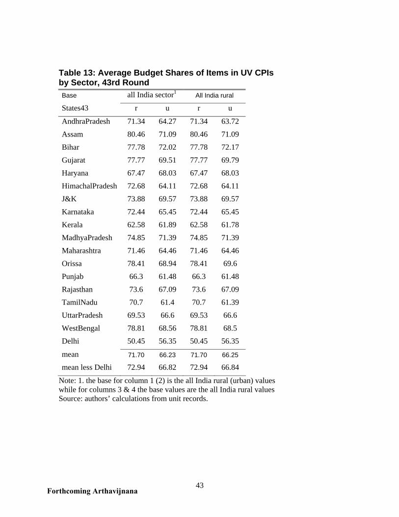
43

Table 13: Average Budget Shares of Items in UV CPIs by Sector, 43rd Round Base all India sector1 All India rural

States43 r u r u

AndhraPradesh 71.34 64.27 71.34 63.72

Assam 80.46 71.09 80.46 71.09

Bihar 77.78 72.02 77.78 72.17

Gujarat 77.77 69.51 77.77 69.79

Haryana 67.47 68.03 67.47 68.03

HimachalPradesh 72.68 64.11 72.68 64.11

J&K 73.88 69.57 73.88 69.57

Karnataka 72.44 65.45 72.44 65.45

Kerala 62.58 61.89 62.58 61.78

MadhyaPradesh 74.85 71.39 74.85 71.39

Maharashtra 71.46 64.46 71.46 64.46

Orissa 78.41 68.94 78.41 69.6

Punjab 66.3 61.48 66.3 61.48

Rajasthan 73.6 67.09 73.6 67.09

TamilNadu 70.7 61.4 70.7 61.39

UttarPradesh 69.53 66.6 69.53 66.6

WestBengal 78.81 68.56 78.81 68.5

Delhi 50.45 56.35 50.45 56.35

mean 71.70 66.23 71.70 66.25

mean less Delhi 72.94 66.82 72.94 66.84

Note: 1. the base for column 1 (2) is the all India rural (urban) values while for columns 3 & 4 the base values are the all India rural values Source: authors’ calculations from unit records.


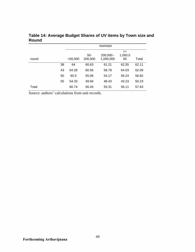
44

Table 14: Average Budget Shares of UV items by Town size and Round townsize

round <50,000 50-

200,000 200,000 - 1,000,000

>= 1,000,0

00 Total

38 64 60.63 61.21 62.55 62.11

43 64.28 60.56 58.78 64.03 62.09

50 60.5 55.06 54.17 56.24 56.82

55 54.33 49.94 48.43 43.23 50.23

Total 60.74 56.43 55.31 56.11 57.63



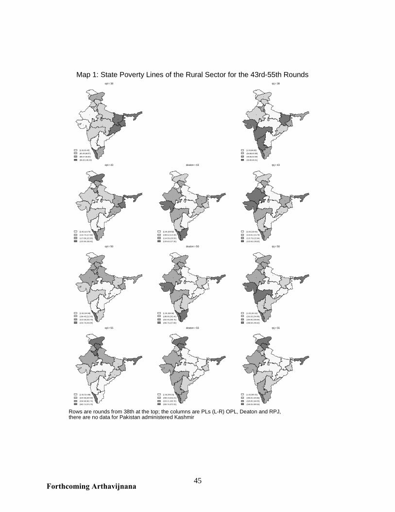
45

[1.00,83.45]

(83.45,88.57]

(88.57,96.82]

(96.82,106.28]

opl r 38

[1.00,84.88]

(84.88,90.85]

(90.85,93.90]

(93.90,96.51]

rpj r 38

[1.00,113.74]

(113.74,117.88]

(117.88,122.90]

(122.90,130.61]

opl r 43

[1.00,108.52]

(108.52,114.39]

(114.39,120.50]

(120.50,127.30]

deaton r 43

[1.00,110.91]

(110.91,115.79]

(115.79,122.64]

(122.64,128.02]

rpj r 43

[1.00,194.49]

(194.49,212.58]

(212.58,233.79]

(233.79,243.84]

opl r 50

[1.00,188.96]

(188.96,202.46]

(202.46,206.76]

(206.76,227.89]

deaton r 50

[1.00,191.63]

(191.63,204.90]

(204.90,209.94]

(209.94,246.62]

rpj r 50

[1.00,314.98]

(314.98,334.98]

(334.98,362.74]

(362.74,374.79]

opl r 55

[1.00,299.19]

(299.19,315.21]

(315.21,335.76]

(335.76,372.33]

deaton r 55

[1.00,305.92]

(305.92,320.85]

(320.85,340.55]

(340.55,383.54]

rpj r 55

Rows are rounds from 38th at the top; the columns are PLs (L-R) OPL, Deaton and RPJ,there are no data for Pakistan administered Kashmir

Map 1: State Poverty Lines of the Rural Sector for the 43rd-55th Rounds


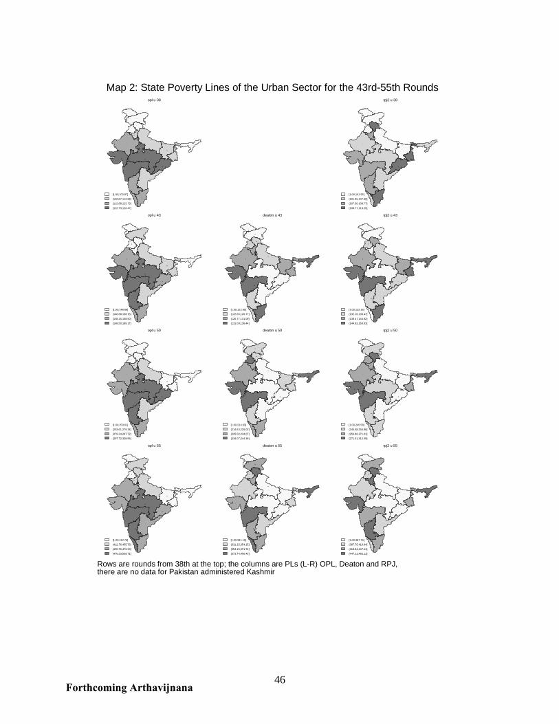
46

[1.00,102.87]

(102.87,112.68]

(112.68,122.73]

(122.73,126.47]

opl u 38

[1.00,101.95]

(101.95,107.30]

(107.30,108.77]

(108.77,118.25]

rpj2 u 38

[1.00,146.68]

(146.68,158.15]

(158.15,168.50]

(168.50,189.17]

opl u 43

[1.00,122.65]

(122.65,126.77]

(126.77,131.09]

(131.09,136.44]

deaton u 43

[1.00,132.16]

(132.16,139.47]

(139.47,144.92]

(144.92,159.93]

rpj2 u 43

[1.00,253.61]

(253.61,279.34]

(279.34,297.72]

(297.72,328.56]

opl u 50

[1.00,214.63]

(214.63,225.02]

(225.02,234.07]

(234.07,244.39]

deaton u 50

[1.00,245.58]

(245.58,256.86]

(256.86,271.01]

(271.01,312.39]

rpj2 u 50

[1.00,412.76]

(412.76,455.76]

(455.76,476.33]

(476.33,539.71]

opl u 55

[1.00,331.15]

(331.15,354.15]

(354.15,371.74]

(371.74,400.43]

deaton u 55

[1.00,387.75]

(387.75,418.84]

(418.84,447.11]

(447.11,482.11]

rpj2 u 55

Rows are rounds from 38th at the top; the columns are PLs (L-R) OPL, Deaton and RPJ,there are no data for Pakistan administered Kashmir

Map 2: State Poverty Lines of the Urban Sector for the 43rd-55th Rounds


Prices, Price Indexes and Poverty Counts in India during ......Prices, Price Indexes and Poverty...

Documents

Transcript of Prices, Price Indexes and Poverty Counts in India during ......Prices, Price Indexes and Poverty...