Price Negotiation and Bargaining Costs∗

Pranav Jindal

Smeal College of Business

The Pennsylvania State University

Peter Newberry

Department of Economics

The Pennsylvania State University

April 2015

Abstract

We study the role of consumers’ psychological bargaining costs associated with the decision

to bargain in a retail setting. First, we use a simple model to show how a retailer’s optimal

pricing strategy (fixed pricing vs. bargaining) varies with consumers’ bargaining costs and

the retailer’s marginal costs. We then prove how these fixed bargaining costs can be non-

parametrically identified separately from bargaining power and marginal utility of income.

Using individual-level data on refrigerator transactions, we find that through bargaining,

consumers keep on average 40% of the available surplus. We estimate an average bargaining

cost of $28, i.e. on average consumers will negotiate prices if they get a discount of more

than $28. While there exists substantial heterogeneity in bargaining costs, these costs

are relatively low as compared to the retailer’s markup; thus, making a hybrid strategy

(where retailers post prices but allow consumers to bargain) more profitable than fixed

pricing. Finally, we provide evidence that ignoring bargaining costs may lead to biased

counterfactual pricing analysis.

Keywords: bargaining, fixed pricing, Nash equilibrium, bargaining costs, price discrimina-

tion

JEL codes: D4, C7, L1

∗We are grateful to Jean-Pierre Dube, Paul Greico, Gunter Hitsch and Carl Mela for helpful comments andsuggestions. We also benefited from the comments of participants and discussants at the 2014 InternationalIndustrial Organization Conference in Chicago, 2014 Marketing Academic Research Colloquium at GeorgetownUniversity, 2014 Marketing Science Conference at Emory University, 2014 Marketing Dynamics Conference atLas Vegas, 2015 UT Dallas FORMS Conference, and seminar participants at University of Pittsburgh, Universityof North Carolina at Chapel Hill, Indian Institute of Management Bangalore, Northwestern University andCarnegie Mellon University. We acknowledge an anonymous retailer for providing data, Pradeep Chintaguntafor financial support in collecting part of the data, and Manpreet Singh for excellent research assistance. Allerrors and omissions are the responsibility of the authors. All correspondence may be addressed to the authorsvia e-mail at pranav.jindal@psu.edu or pwnewberry@psu.edu.

1

1 Introduction

Price negotiation is a common way for individuals to receive a discount off the posted price.

However, not all consumers bargain when given the opportunity.1 For example, consumer

reports indicate that 61% of consumers negotiate prices of goods and services and 33% bargain

for expensive home appliances specifically.23 One explanation for this behavior is that there

exists a cost (henceforth called bargaining cost) to initiate a negotiation. This is the fixed

psychological cost associated with the decision to haggle, and does not influence the negotiated

price (conditional on bargaining).45 In contrast, bargaining power is the relative bargaining

ability of the participants and is the key determinant of the final negotiated price.6 In this

paper, we study the role of consumers’ bargaining cost in a retail setting. Specifically, we

examine how they affect firm profits and optimal pricing policies (i.e., bargaining versus fixed

prices).

In general, the optimality of a bargaining or a fixed pricing strategy is theoretically ambigu-

ous. This ambiguity is evidenced by the variation in pricing policies across industries. Several

business-to-consumer markets such as housing, automobiles, etc., feature price negotiation as

the dominant pricing strategy. By contrast, in markets such as computing equipment, con-

sumer packaged goods, etc., retailers sell products only at posted prices. Pricing policies also

vary across retailers within an industry. For example, in markets such as consumer electronics,

home appliances and used automobiles, some retailers sell at fixed prices, while others allow

negotiation. This implies that the choice of pricing policy is an empirical question which, we

posit, depends crucially on the distribution of consumers’ bargaining costs. The primary goal

of this paper is to demonstrate the importance of these bargaining costs, which we do in three

ways.

First, we use simulation to show how pricing strategy varies with changes in bargaining

costs relative to the available surplus (to be split). We consider a monopolist firm selling to

consumers under two different scenarios: one where consumers are allowed to bargain, and the

other with fixed (take it or leave it) prices. In the scenario where consumers can bargain, the

firm sets a posted price and allows consumers to negotiate a lower price via Nash bargaining.

1In this paper, we use the words price negotiation and bargaining interchangeably. By default, any referenceto these implies negotiation over prices.

2http://www.consumerreports.org/cro/magazine-archive/august-2009/appliances/where-to-buy-appliances/overview/buying-appliances-ov.htm

3http://www.consumerreports.org/cro/magazine/2013/08/how-to-bargain/index.htm4Zeng, Dasgupta, and Weinberg (2007) cite a story in Marketing Magazine August 28, 2000 which found

that 80-86% of car buyers don’t like bargaining.5In a B2B context, bargaining costs are the costs associated with going to the bargaining table (e.g., travel

expenses, legal fees).6Perry (1986), Larsen (2014), Keniston (2011) etc. have studied the role of bargaining cost in determining

negotiation outcomes. In these papers, bargaining cost refers to the cost associated with making offers in eachround and is the same as bargaining ability in our context. Henceforth, bargaining costs will imply the fixedpsychological costs, and bargaining power will imply bargaining ability.

2

We call this a “hybrid” pricing strategy since it incorporates both posted prices and bargaining;

as opposed to a “pure” bargaining strategy, where consumers either negotiate on prices or don’t

purchase at all. This hybrid policy is what is utilized in most retail settings. We also assume

that bargaining is costly, meaning that some consumers may choose to pay the posted price

even though they would receive a lower price by negotiating.

We find that at different levels of bargaining cost, the optimal profit from using the hybrid

policy can be larger than that from setting a fixed price, and vice versa. Additionally, we

find that the difference in profits between the two strategies does not increase (or decrease)

monotonically with bargaining costs. This exercise motivates our empirical analysis in two

ways: it demonstrates the importance of identifying bargaining costs in order to accurately

compare hybrid pricing with fixed pricing, and it introduces an interesting counterfactual

experiment - how does the firm’s optimal pricing strategy change as bargaining cost change

relative to the available surplus.

Next, we quantify bargaining costs using data from a large appliance retailer. We use

individual-level data on purchases of refrigerators to provide model-free evidence that bargain-

ing costs exist, and are at most $40 on average. With an average wholesale cost of $995, and

an average posted price of $1405, the bargaining costs represent around 10% of the available

surplus. Further, reduced-form analysis indicates that retailers have more bargaining power

relative to the consumer. We then specify a structural demand model consistent with Nash

bargaining equilibrium concept, and show bargaining costs can be non-parametrically identi-

fied separately from relative bargaining power, and marginal utility of income. As we highlight

in Section 4.1, the key to separate identification of bargaining costs is our ability to observe

consumers purchasing at both posted prices and bargained prices.

We estimate the model and find substantial heterogeneity (at the zip-code level) in bar-

gaining power and bargaining costs, with the average bargaining cost being $28 and average

relative consumer bargaining power being 0.39. These are in line with the model free results.

We use these demand estimates to calculate optimal prices under hybrid pricing and fixed pric-

ing. We find that for wholesale costs typically observed in the data, it is more profitable for the

retailer to allow bargaining. This is primarily driven by the fact that gains from bargaining far

exceed bargaining costs, and thus, almost all consumers bargain, and the retailer benefits from

discriminating among consumers based on their bargaining power. As the retailer’s marginal

cost increases, the possible gains from bargaining go down relative to the bargaining cost, and

fixed pricing strategy becomes more attractive. This is in line with the simulation results as

adjusting retailer cost (i.e., available surplus) while keeping bargaining cost fixed is equivalent

to adjusting bargaining cost while keeping retailer cost fixed.

Finally, we study how failure to account for bargaining costs leads to biased preference

estimates which has implications for optimal pricing strategy. In a model not allowing for

bargaining costs, consumers seem to be slightly more adept at bargaining (relative to the base

3

case) with an average bargaining power of 0.41. We do not find much of a difference in the

willingness to pay estimates, implying that when bargaining costs are relatively small, ignoring

them may not adjust the retailer’s pricing strategy.

This paper contributes to the marketing and economics literature in several ways. First,

we develop a structural demand model under hybrid pricing and show how bargaining costs,

bargaining power, and marginal utility of income are non-parametrically identified with ob-

servational data. This provides researchers with a framework of how to study bargaining in

the retail industry. Second, we quantify consumers’ bargaining costs using transaction-level

data from a large retailer in the U.S. While we study one market in particular, we believe our

analysis provides general insights on both the effect of introducing a bargaining policy and

the possible reason for the observed variation in policies across markets and retailers. Third,

we demonstrate that bargaining costs are crucial in determining optimal pricing strategy and

firm profitability. To the best of our knowledge, this is the first paper which studies the ef-

fect of consumer bargaining costs on firm pricing strategy. This research is also of interest to

managers of retail firms. There is a recent trend among large retailers to allow consumers to

price negotiate, with some even training their employees in the art of bargaining.7 Even big

online retailers such as Amazon and eBay have started to allow consumers to make offers on a

selection of their products.8 Through our analysis, we shed light on whether such a move will

be profitable in different contexts. Specifically, if retailers can estimate or get a proxy of the

distribution of consumers’ bargaining costs, then comparing these with the available surplus

should provide guidance on the optimal pricing strategy.

The remainder of the paper is organized as follows. Section 2 presents a brief review

of the relevant literature. Section 3 explores a simple theoretical example of a monopolist

under hybrid pricing, while Section 4 specifies the structural demand model and discusses

identification. Sections 5 and 6 introduce the data and the estimation details, while Section 7

presents the results and counterfactual analysis. Finally, section 8 concludes.

2 Literature Review

This research draws from several different strands of literature. First, there are a number

of theoretical papers which examine bargaining as an alternative to fixed pricing. Bester

(1993) studies the connection between quality decisions and the choice of pricing policy in a

competitive environment, while Arnold and Lippman (1998) demonstrate the importance of

the relative bargaining power in the monopolist’s decision of whether or not to negotiate prices.

Wang (1995) examines the role of sellers’ bargaining costs. While these papers compare pure

bargaining to fixed pricing, we study the hybrid bargaining strategy where retailer posts a price

7http://www.nytimes.com/2013/12/16/business/more-retailers-see-haggling-as-a-price-of-doing-business.html

8http://www.consumerreports.org/cro/news/2014/12/haggle-your-way-to-savings-on-amazon/index.htm

4

and then allows negotiation. Chen and Rosenthal (1996), on the other hand, consider a market

in which the seller posts a price, but does so only as a commitment device to attract buyers

who all bargain. Theoretical papers which consider the hybrid model of bargaining include

Desai and Purohit (2004) and Gill and Thanassoulis (2013). They examine the competitive

effects of bargaining when there is only a subset of consumers who negotiate. However, they

do not study the mechanism through which consumers choose whether or not to bargain (e.g.,

bargaining costs). The theoretical models which most closely resembles our set up are that of

Zeng, Dasgupta, and Weinberg (2007) and Cui, Mallucci, and Zhang (2014). Zeng, Dasgupta,

and Weinberg (2007) examine a market in which consumers vary in their bargaining cost. They

find that the hybrid model can be optimal given there are enough “high cost” consumers, but

not too many. We study a similar question as Zeng, Dasgupta, and Weinberg (2007), but do so

empirically. In contrast, Cui, Mallucci, and Zhang (2014) specifically study how hybrid pricing

not only allows price discrimination but also allows retailers to collude on prices.

The empirical work on bargaining is mostly focused on business-to-business markets. Dra-

ganska, Klapper, and Villas-Boas (2009) study the role of firm size, store-brand introductions,

and service-level differentiation in determining the wholesale prices for coffee in the German

market. Crawford and Yurukoglu (2012) examine bargaining between television stations and

cable operators in order to compare a la cart pricing to bundling, whereas Grennan (2013)

focuses on negotiations between hospitals and coronary stent manufacturers to examine the

welfare effects of the bargained prices. Gowrisankaran, Nevo, and Town (2014) estimate the

effects of vertical mergers when prices are negotiated between upstream and downstream firms.

None of these papers consider the role of bargaining costs, which is most likely due to the fact

that bargaining costs and upstream firms marginal costs are not separately identified.

There are a few papers which look at price negotiation in business-to-consumer markets.

Chen, Yang, and Zhao (2008) estimate a structural model where consumers bargain on prices

of new automobiles. The most important way in which our paper differs from Chen, Yang, and

Zhao (2008) is that we observe consumers purchasing at the posted price, which we account

for in our model by including consumer bargaining costs. In another paper studying the

automobile market, Scott-Morton, Silva-Risso, and Zettelmeyer (2011) study the determinants

of bargaining outcomes. Most importantly for our study, they find that “bargaining disutility”

plays a significant role in determining these outcomes. The primary goal of the these papers is

to examine demand with bargained prices, while we focus on quantifying consumer bargaining

costs in order to compare the hybrid pricing to fixed pricing.

Keniston (2011) and Huang (2012) are most similar to our paper in spirit, in that they

both estimate a structural model with bargaining costs to compare pricing policies. However,

these papers differ from ours in several respects, which we discuss in sequence. First, Keniston

(2011) only accounts for the marginal bargaining cost associated with making offers (bargaining

power in our context), and does not look at the fixed costs associated with bargaining, which

5

is the primary objective of this paper. Second, the data used in Keniston (2011) comes from a

field experiment using the auto rickshaw market in India, which allows for some less restrictive

assumptions, such as imperfect information. Finally, bargaining is studied in the context of

the developing world, while we focus on the retail sector in the United States. Huang (2012)

uses aggregate sales data to study why some used car dealerships sell at fixed prices while

others allow consumers to haggle. However, data limitations do not allow the author to model

the exact bargaining process, which makes the joint distribution of bargaining power (discount

offered by seller) and bargaining cost (consumer’s patience) not identified non-parametrically.

In fact, the paper restricts bargaining cost and estimates the discounts dealers offer condi-

tional on this. By contrast, we show that the bargaining parameters are non-parametrically

identified in our data and estimate their joint distribution while allowing for heterogeneity.

Finally, Huang (2012) studies the effect of product differentiation and competition on optimal

pricing policy. We have data from only firm, so instead focus on how the optimal pricing

strategy changes as consumers incentives to bargain vary. This requires individual-level data

on consumers purchasing at both posted prices and negotiated prices, which is not available

to Huang (2012).

3 Importance of Bargaining Costs

In previous research, differences in bargaining power stem from differences in consumer’s (or

retailer’s) bargaining costs i.e., bargaining cost associated with making offers forms the eco-

nomic foundation of bargaining power. This cost is marginal in that it is incurred every time

an offer is made, and can be seen as the patience of the negotiating party i.e., the cost of their

time and effort. In contrast, bargaining costs in our context are the psychological costs asso-

ciated with the decision to bargain or not. Thus, while the consumer may potentially realize

gains from bargaining (subject to a non-zero relative bargaining power), bargaining costs can

offset these gains, resulting in either purchases at posted price or no purchases at all. In other

words, while bargaining power determines how the total gains from trade are split between the

agents, bargaining costs determine whether bargaining occurs or not.

To the extent that the consumer may enjoy the bargaining process, the bargaining cost

may be negative.9 We treat bargaining costs as individual and context dependent preference,

i.e. bargaining costs vary across individuals, and for the same individual, costs associated

with bargaining for a new automobile may differ from those associated with bargaining over a

home appliance. This has an important implication for the identification of bargaining costs.

If consumers always bargain, as in the context of automobile purchases, then bargaining costs

are incurred on each purchase and consequently, are not separately identified from consumers’

9Given the data, in our empirical application, we restrict bargaining costs to be positive i.e. consumer getsdisutility from bargaining (do not like bargaining) if we do not account for the benefit from the reduced price.

6

willingness to pay. Thus, to identify bargaining costs, one needs to observe consumers making

purchases at both posted and bargained prices. Put differently, the data should have enough

variation in product prices and costs such that the benefits from bargaining can be both higher

or lower than the bargaining costs.

To see the distinction between bargaining costs and bargaining power clearly, assume that

consumers’ relative bargaining power follows a normal distribution with average bargaining

power of 0.5, and consumers’ bargaining costs are equal to 0. Figure 1 plots the distribution of

transacted prices for a product with marginal cost of $448 and a posted price of $800. Without

loss of generality, we assume that consumer’s willingness to pay is greater than $800. Note that

in the absence of bargaining costs, all consumers bargain and transacted prices are determined

based on the consumer’s relative bargaining power. Now assume that all consumers incur a

homogeneous cost of $100 if they bargain. Consumers who have low bargaining power and gain

less than $100 from bargaining (right tail of the distribution in Figure 1) will now not bargain

when faced with bargaining costs. Again, assuming consumers’ willingness to pay is greater

than $800, these consumers will buy the product at the posted price. The new distribution

of transacted prices is shown in Figure 2, and has a “gap” in the right tail. This gap in the

distribution of transacted prices points to the presence of, and is key to the identification of

bargaining costs.10

In addition to this gap, the distinction between bargaining costs and bargaining power can

be seen in how the propensity to pay the posted price changes as the price-cost margin (i.e.,

available surplus) changes. Specifically, suppose bargaining costs are zero. Then consumers

who pay the posted price do so because they have zero relative bargaining power. In this

scenario, the number of consumers who pay the posted price does not change with changes in

available surplus. However, in a world with non-zero bargaining costs, the number of consumers

who pay the posted price increases (decreases) as the available surplus decreases (increases).

3.1 Bargaining Model under Hybrid Pricing

To demonstrate the impact of bargaining costs, we present a simple model of bargaining under

hybrid pricing. The objective of this model is two-fold; first, to show the importance of

bargaining costs using data simulated from the model, and second, to motivate the empirical

model outlined in section 4. We assume that consumer i knows the product she is interested

in and her utility is given by

ui = wi − pi (1)

where wi is her willingness-to-pay, which could be a function of both observable and unob-

servable consumer and product characteristics. The consumer has the option of buying the

10Consumers could also pay posted prices if they have no (zero) bargaining ability. However, if we believethat the distribution of bargaining ability is continuous, then the existance of a gap in transacted prices pointsto a non-zero fixed cost of negotiation.

7

product at posted price, or to bargain (by incurring a bargaining cost) and pay the negotiated

price. Let a ∈ {b, nb} denote the consumer’s decision to bargain or not. Thus, the price she

pays, pi, is either the posted price, p, or the realized bargained price, pi. We assume that the

bargained price is the outcome of Nash bargaining, and that agents have complete information

about preferences and costs. The optimal negotiated price solves the Nash bargaining problem:

pi = maxpi

(wi − pi − dci )λ(pi − cf − dr

)1−λ(2)

where dci and dr are the consumer’s and the retailer’s disagreement pay-offs, respectively. cf

is the marginal cost of the retailer, and λi is the relative bargaining power (higher value of

λi indicates that the consumer is more adept at bargaining). We assume that the retailer’s

disagreement pay-offs are zero (dr = 0).11 The consumer’s disagreement pay-off depends

on whether her willingness to pay for the product is greater than the posted price or not.12

Specifically,

dci =

0 ; wi < p

wi − p ; wi ≥ p(3)

Without loss of generality, we normalize the utility from not purchasing the good to 0. In

reality, consumers may have the option of purchasing from other retailers which will change

the disagreement pay-off. We do not have any information about this in the data; and thus,

in the model, we treat no purchase as accounting for the possibility of not purchasing as well

as purchasing at another store. In section 5.4, we discuss the possible implication of this

assumption on preference estimates. Solving equation 2, and using equation 3, the price paid

by the consumer is given by:

pi =

(1− λi) min {wi, p}+ λic

f︸ ︷︷ ︸pi

; a = b

p ; a = nb

(4)

The equation intuitively implies that the consumer will never pay more than her willingness

to pay or the posted price, whichever is lower; thus, inducing the minimum operator in the

bargained price. If she does not bargain, then the transacted price equals the posted price p.

If she bargains, she additionally incurs a bargaining cost of cbi .

The utility the consumer receives from purchasing the product at the posted price is given

by

upi = wi − p (5)

11We discuss this normalization in greater detail in section 5.4.12This implicitly assumes away the role of competition in determining consumer’s disagreement pay-off. We

address this issue in more detail in section 5.4.

8

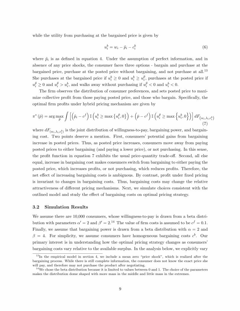
while the utility from purchasing at the bargained price is given by

ubi = wi − pi − cbi (6)

where pi is as defined in equation 4. Under the assumption of perfect information, and in

absence of any price shocks, the consumer faces three options - bargain and purchase at the

bargained price, purchase at the posted price without bargaining, and not purchase at all.13

She purchases at the bargained price if ubi ≥ 0 and ubi ≥ upi , purchases at the posted price if

upi ≥ 0 and upi > ubi , and walks away without purchasing if upi < 0 and ubi < 0.

The firm observes the distribution of consumer preferences, and sets posted price to maxi-

mize collective profit from those paying posted price, and those who bargain. Specifically, the

optimal firm profits under hybrid pricing mechanism are given by

π∗ (p) = arg maxp

∫ [(pi − cf

)I(ubi ≥ max

{upi , 0

})+(p− cf

)I(upi ≥ max

{ubi , 0

})]dF(wi,λi,cbi)

(7)

where dF(wi,λi,cbi ) is the joint distribution of willingness-to-pay, bargaining power, and bargain-

ing cost. Two points deserve a mention. First, consumers’ potential gains from bargaining

increase in posted prices. Thus, as posted price increases, consumers move away from paying

posted prices to either bargaining (and paying a lower price), or not purchasing. In this sense,

the profit function in equation 7 exhibits the usual price-quantity trade-off. Second, all else

equal, increase in bargaining cost makes consumers switch from bargaining to either paying the

posted price, which increases profits, or not purchasing, which reduces profits. Therefore, the

net effect of increasing bargaining costs is ambiguous. By contrast, profit under fixed pricing

is invariant to changes in bargaining costs. Thus, bargaining costs may change the relative

attractiveness of different pricing mechanisms. Next, we simulate choices consistent with the

outlined model and study the effect of bargaining costs on optimal pricing strategy.

3.2 Simulation Results

We assume there are 10,000 consumers, whose willingness-to-pay is drawn from a beta distri-

bution with parameters α′ = 2 and β′ = 2.14 The value of firm costs is assumed to be cf = 0.1.

Finally, we assume that bargaining power is drawn from a beta distribution with α = 2 and

β = 4. For simplicity, we assume consumers have homogeneous bargaining costs cb. Our

primary interest is in understanding how the optimal pricing strategy changes as consumers’

bargaining costs vary relative to the available surplus. In the analysis below, we explicitly vary

13In the empirical model in section 4, we include a mean zero “price shock”, which is realized after thebargaining process. While there is still complete information, the consumer does not know the exact price shewill pay, and therefore may not purchase the product after negotiating.

14We chose the beta distribution because it is limited to values between 0 and 1. The choice of the parametersmakes the distribution dome shaped with more mass in the middle and little mass in the extremes.

9

bargaining cost and study how it affects pricing strategy. However, as we show in section 7.2,

changes in bargaining costs relative to the available surplus can also be achieved by holding

bargaining costs fixed, and changing the retailer’s marginal cost.15

We calculate the optimal posted price and profit based on equation 7. Additionally, we

calculate the optimal price and profit if the firm uses a fixed price. The top panel of Figure

3 plots the percentage of consumers bargaining and paying posted prices for this distribution

of bargaining power. The middle and bottom panels of Figure 3 plot optimal prices and

profits under different pricing strategies as bargaining costs vary relative to available surplus.

For small bargaining costs (relative to the available surplus), it is optimal for the firm to set

posted price corresponding to the highest willingness to pay. Conditional on purchasing, all

consumers bargain (top panel of Figure 3), and the firm extracts more surplus under hybrid

pricing. As relative bargaining cost increases, bargaining becomes unattractive to consumers

with least bargaining power (who gain the least from bargaining). Since these are also the

consumers who are most profitable to the firm, the firm responds by lowering posted prices

to entice them back; thus, optimal posted price falls and the number of consumers who pay

the posted price increases. However, the lost profit from consumers who switch to the outside

option exceeds gains from consumers switching to paying posted prices, and thus, optimal

profits under hybrid pricing fall (left half of the bottom panel of Figure 3).

As relative bargaining costs increase further, consumers with high bargaining power move

away from bargaining. Since these consumers are more profitable to the firm if they pay

posted prices, the losses due to non-purchasers are offset by gains from others paying posted

prices. Therefore, optimal profit is increasing in bargaining costs (middle-third of bottom

panel of Figure 3). As can be seen in the middle panel, the firm responds by increasing the

posted price. This further reduces the number of consumers who bargain until eventually, the

bargaining costs are high enough such that no one bargains. At this point, optimal prices and

profits under the hybrid pricing strategy are the same as under fixed pricing. In summary, as

bargaining costs vary relative to the available surplus, consumers switch between bargaining

and paying posted prices, which changes the attractiveness of bargaining relative to fixed

pricing for the retailer.

This exercise provides two key insights. First, the optimal posted price and profit are

functions of how bargaining costs vary relative to the available surplus, implying failure to

account for them will lead to biased pricing outcomes. Broadly speaking, the magnitude of

bias increases with the magnitude of bargaining costs. Second, the optimal pricing mechanism

depends on the level of bargaining cost. Thus, quantifying bargaining costs is crucial to

comparing alternate pricing mechanisms.

15We study how optimal pricing strategy changes with retailer marginal costs in the counterfactual analysis.

10

4 Empirical Model

We now generalize the model outlined in section 3.1. We assume that a consumer knows

the product she is interested in, and makes bargaining and purchasing decisions only for this

product. Let a ∈ {b, nb} indicate a consumer’s decision to bargain or not. The utility consumer

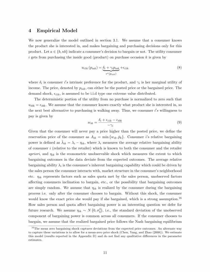
i gets from purchasing the inside good (product) on purchase occasion k is given by

ui1k (piak) = δi + γipiak︸ ︷︷ ︸v∗(piak)

+εi1k (8)

where δi is consumer i′s intrinsic preference for the product, and γi is her marginal utility of

income. The price, denoted by piak, can either be the posted price or the bargained price. The

demand shock, εi1k, is assumed to be i.i.d type one extreme value distributed.

The deterministic portion of the utility from no purchase is normalized to zero such that

ui0k = εi0k. We assume that the consumer knows exactly what product she is interested in, so

the next best alternative to purchasing is walking away. Thus, we consumer i′s willingness to

pay is given by

wik =δi + εi1k − εi0k

−γi(9)

Given that the consumer will never pay a price higher than the posted price, we define the

reservation price of the consumer as Aik = min {wik, pk}. Consumer i’s relative bargaining

power is defined as λik = λi − ηik, where λi measures the average relative bargaining ability

of consumer i (relative to the retailer) which is known to both the consumer and the retailer

apriori, and ηik is the econometric unobservable shock which measures the extent to which

bargaining outcomes in the data deviate from the expected outcomes. The average relative

bargaining ability λi is the consumer’s inherent bargaining capability which could be driven by

the sales person the consumer interacts with, market structure in the consumer’s neighborhood

etc. ηik represents factors such as sales quota met by the sales person, unobserved factors

affecting consumers inclination to bargain, etc., or the possibility that bargaining outcomes

are simply random. We assume that ηik is realized by the consumer during the bargaining

process i.e. only after the consumer chooses to bargain. Without this shock, the consumer

would know the exact price she would pay if she bargained, which is a strong assumption.16

How sales person and quota affect bargaining power is an interesting question we defer for

future research. We assume ηik ∼ N(0, σ2

η

), i.e., the standard deviation of the unobserved

component of bargaining power is common across all consumers. If the consumer chooses to

bargain, we assume that the realized bargained price follows the Nash bargaining equilibrium

16The mean zero bargaining shock captures deviations from the expected price outcomes. An alternate wayto capture these variations is to allow for a mean-zero price shock (Chen, Yang, and Zhao (2008)). We estimatethis model (results reported in the Appendix D) and do not find any qualitative differences in the parameterestimates.

11

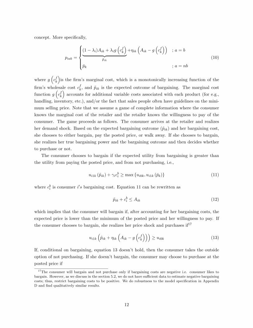
concept. More specifically,

piak =

(1− λi)Aik + λig

(cfk

)︸ ︷︷ ︸

pik

+ηik

(Aik − g

(cfk

)); a = b

pk ; a = nb

(10)

where g(cfk

)is the firm’s marginal cost, which is a monotonically increasing function of the

firm’s wholesale cost cfk , and pik is the expected outcome of bargaining. The marginal cost

function g(cfk

)accounts for additional variable costs associated with each product (for e.g.,

handling, inventory, etc.), and/or the fact that sales people often have guidelines on the mini-

mum selling price. Note that we assume a game of complete information where the consumer

knows the marginal cost of the retailer and the retailer knows the willingness to pay of the

consumer. The game proceeds as follows. The consumer arrives at the retailer and realizes

her demand shock. Based on the expected bargaining outcome (pik) and her bargaining cost,

she chooses to either bargain, pay the posted price, or walk away. If she chooses to bargain,

she realizes her true bargaining power and the bargaining outcome and then decides whether

to purchase or not.

The consumer chooses to bargain if the expected utility from bargaining is greater than

the utility from paying the posted price, and from not purchasing, i.e.,

ui1k (pik) + γicbi ≥ max {ui0k, ui1k (pk)} (11)

where cbi is consumer i′s bargaining cost. Equation 11 can be rewritten as

pik + cbi ≤ Aik (12)

which implies that the consumer will bargain if, after accounting for her bargaining costs, the

expected price is lower than the minimum of the posted price and her willingness to pay. If

the consumer chooses to bargain, she realizes her price shock and purchases if17

ui1k

(pik + ηik

(Aik − g

(cfk

)))≥ ui0k (13)

If, conditional on bargaining, equation 13 doesn’t hold, then the consumer takes the outside

option of not purchasing. If she doesn’t bargain, the consumer may choose to purchase at the

posted price if

17The consumer will bargain and not purchase only if bargaining costs are negative i.e. consumer likes tobargain. However, as we discuss in the section 5.2, we do not have sufficient data to estimate negative bargainingcosts; thus, restrict bargaining costs to be positive. We do robustness to the model specification in AppendixD and find qualitatively similar results.

12

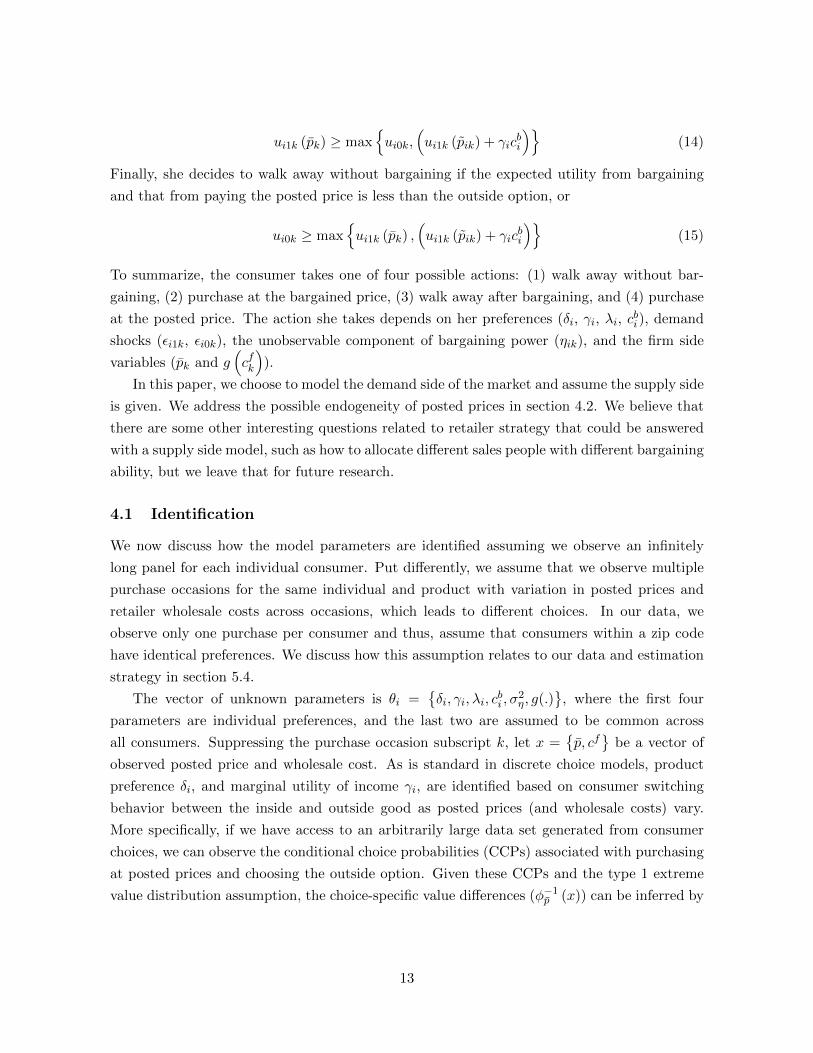
ui1k (pk) ≥ max{ui0k,

(ui1k (pik) + γic

bi

)}(14)

Finally, she decides to walk away without bargaining if the expected utility from bargaining

and that from paying the posted price is less than the outside option, or

ui0k ≥ max{ui1k (pk) ,

(ui1k (pik) + γic

bi

)}(15)

To summarize, the consumer takes one of four possible actions: (1) walk away without bar-

gaining, (2) purchase at the bargained price, (3) walk away after bargaining, and (4) purchase

at the posted price. The action she takes depends on her preferences (δi, γi, λi, cbi), demand

shocks (εi1k, εi0k), the unobservable component of bargaining power (ηik), and the firm side

variables (pk and g(cfk

)).

In this paper, we choose to model the demand side of the market and assume the supply side

is given. We address the possible endogeneity of posted prices in section 4.2. We believe that

there are some other interesting questions related to retailer strategy that could be answered

with a supply side model, such as how to allocate different sales people with different bargaining

ability, but we leave that for future research.

4.1 Identification

We now discuss how the model parameters are identified assuming we observe an infinitely

long panel for each individual consumer. Put differently, we assume that we observe multiple

purchase occasions for the same individual and product with variation in posted prices and

retailer wholesale costs across occasions, which leads to different choices. In our data, we

observe only one purchase per consumer and thus, assume that consumers within a zip code

have identical preferences. We discuss how this assumption relates to our data and estimation

strategy in section 5.4.

The vector of unknown parameters is θi ={δi, γi, λi, c

bi , σ

2η, g(.)

}, where the first four

parameters are individual preferences, and the last two are assumed to be common across

all consumers. Suppressing the purchase occasion subscript k, let x ={p, cf

}be a vector of

observed posted price and wholesale cost. As is standard in discrete choice models, product

preference δi, and marginal utility of income γi, are identified based on consumer switching

behavior between the inside and outside good as posted prices (and wholesale costs) vary.

More specifically, if we have access to an arbitrarily large data set generated from consumer

choices, we can observe the conditional choice probabilities (CCPs) associated with purchasing

at posted prices and choosing the outside option. Given these CCPs and the type 1 extreme

value distribution assumption, the choice-specific value differences (φ−1p (x)) can be inferred by

13

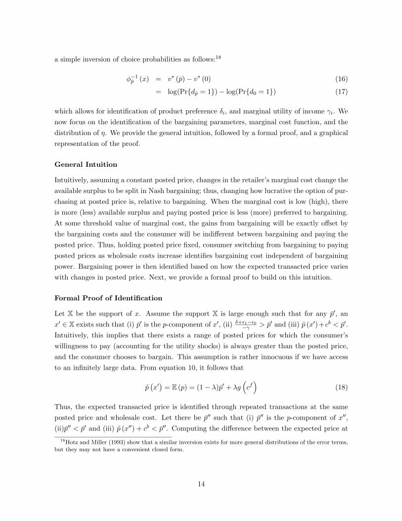
a simple inversion of choice probabilities as follows:18

φ−1p (x) = v∗ (p)− v∗ (0) (16)

= log(Pr{dp = 1})− log(Pr{d0 = 1}) (17)

which allows for identification of product preference δi, and marginal utility of income γi. We

now focus on the identification of the bargaining parameters, marginal cost function, and the

distribution of η. We provide the general intuition, followed by a formal proof, and a graphical

representation of the proof.

General Intuition

Intuitively, assuming a constant posted price, changes in the retailer’s marginal cost change the

available surplus to be split in Nash bargaining; thus, changing how lucrative the option of pur-

chasing at posted price is, relative to bargaining. When the marginal cost is low (high), there

is more (less) available surplus and paying posted price is less (more) preferred to bargaining.

At some threshold value of marginal cost, the gains from bargaining will be exactly offset by

the bargaining costs and the consumer will be indifferent between bargaining and paying the

posted price. Thus, holding posted price fixed, consumer switching from bargaining to paying

posted prices as wholesale costs increase identifies bargaining cost independent of bargaining

power. Bargaining power is then identified based on how the expected transacted price varies

with changes in posted price. Next, we provide a formal proof to build on this intuition.

Formal Proof of Identification

Let X be the support of x. Assume the support X is large enough such that for any p′, an

x′ ∈ X exists such that (i) p′ is the p-component of x′, (ii) δ+ε1−ε0−γ > p′ and (iii) p (x′)+cb < p′.

Intuitively, this implies that there exists a range of posted prices for which the consumer’s

willingness to pay (accounting for the utility shocks) is always greater than the posted price,

and the consumer chooses to bargain. This assumption is rather innocuous if we have access

to an infinitely large data. From equation 10, it follows that

p(x′)

= E (p) = (1− λ)p′ + λg(cf)

(18)

Thus, the expected transacted price is identified through repeated transactions at the same

posted price and wholesale cost. Let there be p′′ such that (i) p′′ is the p-component of x′′,

(ii)p′′ < p′ and (iii) p (x′′) + cb < p′′. Computing the difference between the expected price at

18Hotz and Miller (1993) show that a similar inversion exists for more general distributions of the error terms,but they may not have a convenient closed form.

14

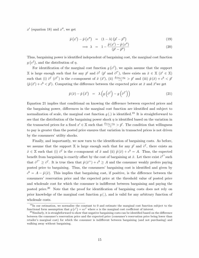
x′ (equation 18) and x′′, we get

p(x′)− p

(x′′)

= (1− λ)(p′ − p′′

)(19)

=⇒ λ = 1− p (x′)− p (x′′)

(p′ − p′′)(20)

Thus, bargaining power is identified independent of bargaining cost, the marginal cost function

g(cf), and the distribution of η.

For identification of the marginal cost function g(cf), we again assume that the support

X is large enough such that for any p′ and cf (p′ and cf′), there exists an x ∈ X (x′ ∈ X)

such that (i) cf (cf′) is the c-component of x (x′), (ii) δ+ε1−ε0

−γ > p′ and (iii) p (x) + cb < p′

(p (x′) + cb < p′). Computing the difference between the expected price at x and x′we get

p (x)− p(x′)

= λ(g(cf)− g

(cf′))

(21)

Equation 21 implies that conditional on knowing the difference between expected prices and

the bargaining power, differences in the marginal cost function are identified and subject to

normalization of scale, the marginal cost function g (.) is identified.19 It is straightforward to

see that the distribution of the bargaining power shock η is identified based on the variation in

the transacted prices for a fixed x′ ∈ X such that δ+ε1−ε0−γ > p′. The condition that willingness

to pay is greater than the posted price ensures that variation in transacted prices is not driven

by the consumers’ utility shocks.

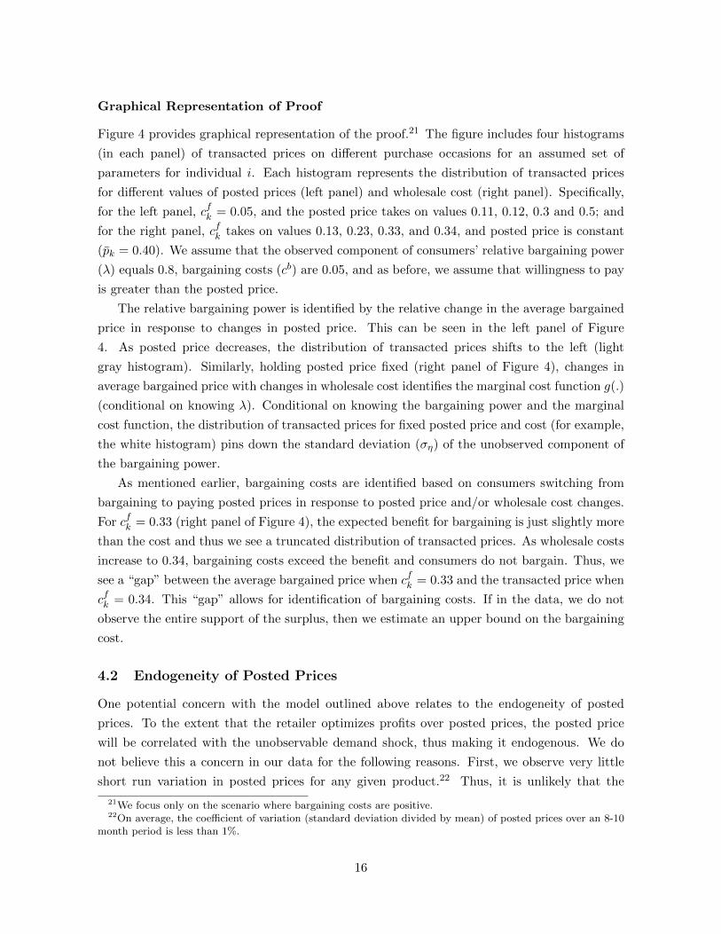
Finally, and importantly, we now turn to the identification of bargaining costs. As before,

we assume that the support X is large enough such that for any p′ and cf , there exists an

x ∈ X such that (i) cf is the c-component of x and (ii) p (x) + cb = A. Thus, the expected

benefit from bargaining is exactly offset by the cost of bargaining at x. Let there exist cf+

such

that cf+ ≥ cf . It is true then that p (x+) + cb ≥ A and the consumer weakly prefers paying

posted price to bargaining. Thus, the consumers’ bargaining cost is identified and given by

cb = A − p (x). This implies that bargaining cost, if positive, is the difference between the

consumers’ reservation price and the expected price at the threshold value of posted price

and wholesale cost for which the consumer is indifferent between bargaining and paying the

posted price.20 Note that the proof for identification of bargaining costs does not rely on

prior knowledge of the marginal cost function g (.), and is valid for any arbitrary function of

wholesale costs.

19In our estimation, we normalize the constant to 0 and estimate the marginal cost function subject to thefunctional form assumption that g

(cf)

= κcf where κ is the marginal cost coefficient of interest.20Similarly, it is straightforward to show that negative bargaining costs can be identified based on the difference

between the consumer’s reservation price and the expected price (consumer’s reservation price being lower thanretailer’s marginal cost) for which the consumer is indifferent between bargaining (and not purchasing) andwalking away without bargaining.

15

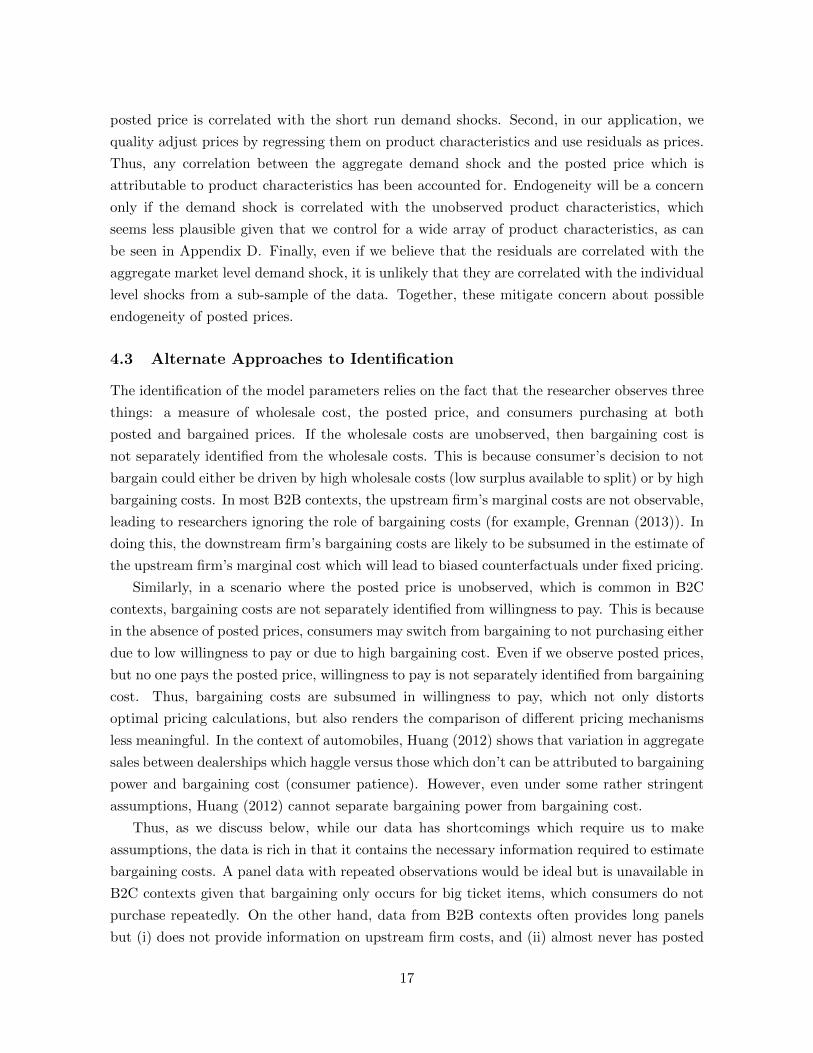
Graphical Representation of Proof

Figure 4 provides graphical representation of the proof.21 The figure includes four histograms

(in each panel) of transacted prices on different purchase occasions for an assumed set of

parameters for individual i. Each histogram represents the distribution of transacted prices

for different values of posted prices (left panel) and wholesale cost (right panel). Specifically,

for the left panel, cfk = 0.05, and the posted price takes on values 0.11, 0.12, 0.3 and 0.5; and

for the right panel, cfk takes on values 0.13, 0.23, 0.33, and 0.34, and posted price is constant

(pk = 0.40). We assume that the observed component of consumers’ relative bargaining power

(λ) equals 0.8, bargaining costs (cb) are 0.05, and as before, we assume that willingness to pay

is greater than the posted price.

The relative bargaining power is identified by the relative change in the average bargained

price in response to changes in posted price. This can be seen in the left panel of Figure

4. As posted price decreases, the distribution of transacted prices shifts to the left (light

gray histogram). Similarly, holding posted price fixed (right panel of Figure 4), changes in

average bargained price with changes in wholesale cost identifies the marginal cost function g(.)

(conditional on knowing λ). Conditional on knowing the bargaining power and the marginal

cost function, the distribution of transacted prices for fixed posted price and cost (for example,

the white histogram) pins down the standard deviation (ση) of the unobserved component of

the bargaining power.

As mentioned earlier, bargaining costs are identified based on consumers switching from

bargaining to paying posted prices in response to posted price and/or wholesale cost changes.

For cfk = 0.33 (right panel of Figure 4), the expected benefit for bargaining is just slightly more

than the cost and thus we see a truncated distribution of transacted prices. As wholesale costs

increase to 0.34, bargaining costs exceed the benefit and consumers do not bargain. Thus, we

see a “gap” between the average bargained price when cfk = 0.33 and the transacted price when

cfk = 0.34. This “gap” allows for identification of bargaining costs. If in the data, we do not

observe the entire support of the surplus, then we estimate an upper bound on the bargaining

cost.

4.2 Endogeneity of Posted Prices

One potential concern with the model outlined above relates to the endogeneity of posted

prices. To the extent that the retailer optimizes profits over posted prices, the posted price

will be correlated with the unobservable demand shock, thus making it endogenous. We do

not believe this a concern in our data for the following reasons. First, we observe very little

short run variation in posted prices for any given product.22 Thus, it is unlikely that the

21We focus only on the scenario where bargaining costs are positive.22On average, the coefficient of variation (standard deviation divided by mean) of posted prices over an 8-10

month period is less than 1%.

16

posted price is correlated with the short run demand shocks. Second, in our application, we

quality adjust prices by regressing them on product characteristics and use residuals as prices.

Thus, any correlation between the aggregate demand shock and the posted price which is

attributable to product characteristics has been accounted for. Endogeneity will be a concern

only if the demand shock is correlated with the unobserved product characteristics, which

seems less plausible given that we control for a wide array of product characteristics, as can

be seen in Appendix D. Finally, even if we believe that the residuals are correlated with the

aggregate market level demand shock, it is unlikely that they are correlated with the individual

level shocks from a sub-sample of the data. Together, these mitigate concern about possible

endogeneity of posted prices.

4.3 Alternate Approaches to Identification

The identification of the model parameters relies on the fact that the researcher observes three

things: a measure of wholesale cost, the posted price, and consumers purchasing at both

posted and bargained prices. If the wholesale costs are unobserved, then bargaining cost is

not separately identified from the wholesale costs. This is because consumer’s decision to not

bargain could either be driven by high wholesale costs (low surplus available to split) or by high

bargaining costs. In most B2B contexts, the upstream firm’s marginal costs are not observable,

leading to researchers ignoring the role of bargaining costs (for example, Grennan (2013)). In

doing this, the downstream firm’s bargaining costs are likely to be subsumed in the estimate of

the upstream firm’s marginal cost which will lead to biased counterfactuals under fixed pricing.

Similarly, in a scenario where the posted price is unobserved, which is common in B2C

contexts, bargaining costs are not separately identified from willingness to pay. This is because

in the absence of posted prices, consumers may switch from bargaining to not purchasing either

due to low willingness to pay or due to high bargaining cost. Even if we observe posted prices,

but no one pays the posted price, willingness to pay is not separately identified from bargaining

cost. Thus, bargaining costs are subsumed in willingness to pay, which not only distorts

optimal pricing calculations, but also renders the comparison of different pricing mechanisms

less meaningful. In the context of automobiles, Huang (2012) shows that variation in aggregate

sales between dealerships which haggle versus those which don’t can be attributed to bargaining

power and bargaining cost (consumer patience). However, even under some rather stringent

assumptions, Huang (2012) cannot separate bargaining power from bargaining cost.

Thus, as we discuss below, while our data has shortcomings which require us to make

assumptions, the data is rich in that it contains the necessary information required to estimate

bargaining costs. A panel data with repeated observations would be ideal but is unavailable in

B2C contexts given that bargaining only occurs for big ticket items, which consumers do not

purchase repeatedly. On the other hand, data from B2B contexts often provides long panels

but (i) does not provide information on upstream firm costs, and (ii) almost never has posted

17

prices with purchases always made at negotiated prices.

5 Data and Model-Free Evidence

The data for this study come from a large mid-western appliance retailer. This is a family

owned store and the retailer does not have any other branches. Additionally, the retailer sells

products through its own online portal. The retailer sets a posted price, both in store and

online, but in the store, allows consumers to negotiate on price. Price negotiation at retailers

is not common in the United States, but occurs more frequently for big ticket items. The

market for appliances, specifically, is a market in which price negotiation, or haggling, is often

acceptable. We have a random sample of individual level transactions for products across 13

different categories. The transactions occurred from 2009-2010 and include categories such

as refrigerators, wall ovens, microwaves, dishwashers, etc. In this study, we focus on sales

of refrigerators since it is the most popular product category.23 Additionally, we know from

the retailer that 85% of all the consumers who come to the store to purchase a refrigerator

do so. As we mention in section 6, we use data on purchases in other categories to compute

zip-code level no purchase shares which aides demand estimation. Note that the data does

not provide any information on whether non-purchasers bargained or not. Thus, we cannot

estimate negative bargaining costs, and focus only on the scenario where bargaining costs are

positive.

For each transaction, we observe the product SKU, price paid, wholesale cost of the retailer,

and price of the warranty, if purchased.24 Additionally, we have unique consumer identifier

and information on their zip-code. We supplement this data with posted prices, which were

collected by scraping the retailer’s website. This assumes that the prices shown on the retailer’s

website equal posted prices at the store, which would be violated if the firm price discriminates

between online and offline consumers. In our discussions, the retailer revealed that the posted

prices are the same in store and online. Also, the fact that we observe some consumers

buying at the scraped prices, and that the transacted prices are always lower than the scraped

prices provides additional support against channel based price discrimination. Additionally,

we assume that the highest scraped price for a product is the posted price for the entire sample

period. This assumption is justified by the fact that the average coefficient of variation for

prices over time is less than 1%, implying little variation in posted prices over time.25 While

the posted prices for a given refrigerator are constant, we do see variation in wholesale costs

23Nearly 15% of the transactions in our data are for refrigerators, making up about 35% of total revenue.24Consumers may sometimes negotiate not on product price, but other features such as warranty, free shipping

etc. While we do not observe the shipping fee, we exclude all observations where warranties are purchased eitherfor free or at heavily discounted prices.

25Unlike electronic goods, for home appliances, retailers typically do not engage in price skimming. It is acommon practice to hold prices fixed, and only offer temporary discounts during holidays.

18

which crucially provides the within-product variation in available surplus required to estimate

bargaining costs.

Our data consists of 1541 transactions for over 400 unique refrigerators. Consumers are

spread across 189 different zip-codes with an average of 8 observations per zip-code. For the

structural estimation (results reported in section 7), we focus on zip-codes where we observe

consumers paying both posted and bargained prices, which results in 866 observations from 90

zip-codes.26 For these 90 zip codes, 15% of the purchases are made at posted prices. To account

for the large number of SKUs, we stack posted prices, wholesale costs and transacted prices

and regress them on product characteristics to get quality adjusted prices. In our analysis, we

utilize variation in these quality adjusted prices for the standardized product. Thus, unlike

standard panel data where researchers utilize variation in prices over time, we utilize variation

in posted prices, costs and transacted prices for the standardized product. Estimates from the

pricing regression which quality-adjusts prices are reported in Appendix A. The regression is

based on 2351 observations which we get by stacking unique transacted prices, posted prices

and wholesale costs by product. An R-square of 93% implies that the characteristics capture

substantial variation in prices and costs; and thus, the quality adjusted prices are sensible.27

While this data poses some restrictions which we discuss in section 5.4, the data has a

few nice features. First, and most importantly, we observe consumers purchasing at both

posted prices and bargained prices, which facilitates the identification of bargaining costs.

Second, we observe the retailer’s wholesale cost, which in theory, provides a direct measure

of marginal cost. Third, we have individual level transactions, which is crucial to estimating

the distribution of consumers’ bargaining power and aides estimation of consumers’ bargaining

costs.

5.1 Evidence of Bargaining and Descriptive Statistics

Discussions with the retailer revealed that they encourage consumers to negotiate on prices,

and that negotiation occurs quite frequently. While this provides anecdotal evidence that

consumers bargain, we provide further evidence that the distribution of prices observed in the

data is driven by bargaining as opposed to quantity discounts or other forms of promotions.

Figure 5 shows the distribution of transacted prices for four different refrigerators. We find

substantial variation in transacted prices, especially given that the posted prices (indicated by

the vertical line) of refrigerators do not vary much over time . Though unlikely, the distribution

of transacted prices could be driven by quantity discounts and/or seasonal promotions. To

explore this, we regress the discount the consumer receives (both in dollars and as a percent

26Using data on 189 zip-codes results in lower bargaining power (as expected) but provides identical estimatesfor other preferences (Appendix D).

27In Appendix D, we report results from the model estimated on data where prices are computed basedon regressions involving only either posted prices, or wholesale costs. We do not find any affect of how westandardize prices on preference estimates.

19

of the posted price) on the number of products the consumer purchased in addition to the

refrigerator, and monthly fixed effects which capture possible variation in prices due to seasonal

promotions.

Table 1 reports estimates from these regressions. First, note that barring the October fixed

effect in columns 3 and 4, neither the number of products nor any of the month fixed effects

are significant in explaining the discount consumers receive. If we believe that the distribution

of transacted prices is a result of quantity discounts or seasonal promotions, then these should

be significant in predicting the transacted prices. Further, in the absence of bargaining, the

number of products purchased and time fixed effects should explain almost all of the variation

in prices. In contrast, the number of products purchased and time fixed effects explain only

0.8% of the variation in transacted prices. Controlling for product characteristics increases

the model R-square to 57% (15%) for dollar (percent) discounts; still leaving a substantial

variation in transacted prices. This provides evidence that the distribution of observed prices

is generated from bargaining as opposed to temporary discounts or promotions.28 Another

possible explanation for the observed distribution of prices is that salespeople offer consumers

a discount (based on observable consumer characteristics) immediately when they walk in the

door (i.e., price discrimination without bargaining). Under this scenario, we would mistakenly

assume that the transacted price is the outcome of a bargaining process when in fact, consumers

did not haggle. While we cannot directly test for this in the data, we take the conversations

with the retailer as anecdotal evidence that this is not driving the observed price distribution.

In Table 2, we report descriptive statistics from the data based on 189 zip-codes. Nearly

92% of the consumers purchase at bargained prices, earning an average discount of 12% off the

posted price. This suggests that the average consumer should bargain as long as her bargaining

cost is lower than $173. Further, the fact that 8% of the consumers pay posted prices points to

relatively low, but non-zero, bargaining costs. A high standard deviation of bargaining discount

indicates heterogeneity in consumers’ bargaining power. On average, the posted prices imply a

mark-up of roughly 29% over the wholesale cost. We see substantial variation in posted prices,

wholesale costs and mark-ups across different products and transactions, which is crucial to

estimating product and price preferences. The realized mark-up for bargained products is

around 20% implying that the retailer enjoys a slightly higher relative bargaining power as

compared to the consumer. Figure 6 shows the distribution of discounts for different brands of

refrigerators. The distribution is fairly similar across brands indicating that all brands are sold

at both posted and bargained prices, which alleviates concerns related to minimum advertised

price (MAP) and resale price maintenance (RPM), which are common practices in the home

appliance industry.29

28We get qualitatively similar results if instead of month fixed effects, we regress the dollar discount (orpercent discount) on weekly fixed effects.

29Brand specific regressions confirm that products are not sold at posted prices initially, and then bargainedupon later. This holds true even for Sub-Zero, which has a higher share of transactions at posted prices. Results

20

The retailer indicated that around 15% of consumers who walk in to the store looking for

a refrigerator decide to not buy.30 Using this percentage and the total number of transactions

in our data, we calculate that there are 272 consumers who choose the outside good instead of

one of the in-store refrigerators. The outside good could be a consumer sticking with her old

refrigerator or buying at another retailer. The fact that this is neither at the consumer nor

the product level is a weakness of our data. In sections 5.4 and 6, we discuss the assumptions

we make in order to estimate demand by combining this aggregate share with individual level

transactions data.

5.2 Bargaining Power and Bargaining Cost

We use data on posted and transacted prices to show preliminary model-free evidence of

the existence (and magnitude) of bargaining power and bargaining costs. We assume that

consumers’ willingness to pay is higher than the posted price, and the firm marginal cost

equals the wholesale cost.31 Utilizing this, and re-arranging the terms of equation 10 (ignoring

the k subscript), consumers bargaining power can be written as

λi =p− pip− cf

Higher values of λ imply consumers have higher bargaining power. Figure 7 plots the

distribution of individual consumer bargaining power as inferred from data. First, while we

find substantial heterogeneity in bargaining power, the average consumer bargaining power is

around 0.40. Second, we do not observe any values between 0 and roughly 0.05. This represents

consumers with low bargaining power who did not receive a big enough discount to rationalize

bargaining. We see this as evidence in favor of existence of bargaining cost.

Next, we assume homogeneity in bargaining power within a zip-code, allowing us to sep-

arate the effect of unobservable component of bargaining power. Conditional on the zip-code

level homogeneity in bargaining power, deviations from the expected transacted prices within

the zip-code are driven by the unobserved component. Therefore, in Figure 8, we plot the

distribution of average bargaining power at the zip-code level for all zip-codes that have at

least 5 purchases. The minimum of this distribution is around 0.26, which, again, suggests

that bargaining costs play a role. Consistent with Figure 7, the average bargaining power is

0.41, indicating that the firm has more bargaining power.

In order to take a first look at bargaining costs, note that there is substantial variation

in the transacted prices for each model in Figure 5. Based on the identification discussion in

the preceding section, bargaining cost induces a ’gap’ in transacted prices around the posted

for these regressions can be requested from the authors.30Based on foot-falls and traffic counters, the store owner indicated that the percentage of no purchasers for

refrigerators is between 10 and 20 percent. We therefore take the midpoint of this range.31Assuming willingness to pay is higher than posted price provides an upper bound on the bargaining power.

21

price. For all but one of the SKUs, there exists a ’gap’ between the highest bargained price

and the highest transacted price. Under homogeneity and assuming no deviations from the

expected outcome, the size of this ’gap’ identifies an upper bound on bargaining cost. Given

that we do not have sufficient transactions for each SKU, we pool data across SKUs to get a

model-free estimate of bargaining cost. We follow our discussion from section 4.1, and assume

that bargaining costs are homogeneous within a zip-code. With a large enough sample size, the

bargaining cost within a zip-code can be approximated to mini∈z(p− pi). Figure 9 presents the

distribution of zip-code level bargaining costs based on all zip-codes with at least 5 transactions.

The average bargaining cost across zip-codes has an upper bound of $39 or around 10% of the

average mark-up. We see substantial heterogeneity in bargaining cost with estimated cost is

as low as $11 and as high as $250.

5.3 Evidence of the Structural Model

We now present evidence that the structural model outlined in section 4 is an accurate descrip-

tion of the data generating process. First, we test the Nash bargaining equilibrium concept by

regressing transacted prices on posted prices and wholesale costs. This can be viewed as the

reduced form of the bargaining outcome. Specifically, we run the following regression:

pik = β0 + β1Xk + β2pk + β3cfk + εik

where Xk is a vector of observed attributes of product k.32 According to Nash bargaining, p

and cf should positively affect the transacted price. Results from the regression are reported

in the first column of Table 3. The coefficients on posted price and the marginal cost are

positive, between 0 and 1 and statistically significant. Further, their sum is not significantly

different from 1. This is in line with the predictions of the structural model. The estimates

imply that a $1 increase in wholesale cost leads to a $0.63 increase in the transacted price

which is consistent with estimates of consumer bargaining power in Figures 7 and 8.

Second, assuming willingness to pay is greater than the posted price, the model implies

that consumers prefer bargaining to paying the posted price if pik + cbi < pk. This implies that

in the presence of bargaining costs, conditional on purchase, the probability that a consumer

bargains is increasing in the posted price and decreasing in the wholesale cost. The second

column of Table 3 reports results from the following probit model:

Pr(aik = b) = β0 + β1Xk + β2pk + β3cfk + εik

where aik ∈ {b, nb} indicates whether consumer i bargains on product k or not. As expected,

posted price (wholesale cost) has a positive (negative) and significant effect on the probability

32These attributes are also used to quality-adjust prices and are listed in Table 7 in the appendix.

22

to bargain pointing to the presence of consumer bargaining costs. Together, these two results

provide evidence that the data supports the reduced form of the structural model.

5.4 Identification Assumptions

The identification proof outlined in section 4.1 relies on observing multiple purchase occasions

for the same consumer. Refrigerators are durable goods, and thus, we are unlikely to observe

repeated purchases in any decently long panel data. Therefore, we assume that all consumers

in a zip code have identical deterministic preferences i.e. we assume homogeneity at the zip

code level. In the data, each consumer purchases in an average of 1.44 product categories and

places an average of 1.07 orders. Thus, pooling transactions across different product categories

does not create a panel, which could potentially have been used to relax the homogeneity

assumption. Further, as we detail in section 6, we also require preferences to be homogeneous

within a zip code to account for the zip code level no purchase probabilities. Conditional

on bargaining costs being positive, if consumers within a zip-code are heterogeneous in their

bargaining cost, we will infer the bargaining cost corresponding to the consumer with the

lowest bargaining cost. Thus, our estimate at the zip-code level will be a lower bound on

bargaining cost. Having said this, some consumers in the zip-code may get positive utility just

from bargaining. Given that the data does not allow for identification of negative bargaining

costs, restricting these consumers to have positive bargaining costs will result in an upward

bias in the estimate of bargaining cost. Taken together, the net effect of assuming homogeneity

in preferences within a zip-code on bargaining power is ambiguous, and it’s possible that these

effects may offset each other providing a consistent estimate of bargaining cost. Additionally,

if consumers vary in their expected bargaining power (within a zip-code), then non-purchasers

are likely to be worse at bargaining. Not accounting for this, and in the absence of any

parametric assumptions, we will overestimate consumers’ bargaining power i.e. our estimate

of consumer’s bargaining power will be based only on purchasers and will be upward biased.

Parametric assumptions such as assuming that the observed distribution of bargaining power

follow a continuous distribution allow us to provide a more consistent estimate of bargaining

power.

We make two additional assumptions in our model - a consumer’s disagreement pay-off is

independent of competition (depends only on utility from not purchasing or from purchasing

at the posted price from the same retailer), and that the retailer’s disagreement pay-off is zero

i.e. the retailer can always sell the product to an identical consumer (or a consumer from the

same zip-code). As mentioned in section 4, a consumer’s disagreement pay-off may also depend

on utility from purchasing at another store. Addressing the role of competition would require

explicitly modeling an oligopoly which is not possible given the data. An alternate reduced

form approach would be to allow consumer’s disagreement pay-off to be a function of price at

other stores. While we do not have data on prices at other stores, as we show in Appendix C,

23

this does not bias our estimates of bargaining power and bargaining cost. Finally, the retailer’s

disagreement pay-off may depend on the retailers’ beliefs about the likelihood of selling the

same product to another consumer at a lower, higher or equal price. Endogenously accounting

for the retailer’s beliefs as posted price changes is out of scope of current paper. Instead, in

Appendix C, we show how prior knowledge of (exogenous) retailer’s disagreement pay-off is

not necessary for consistent estimation of bargaining power and bargaining costs.

To summarize, assuming homogeneity in preferences within a zip-code, and not accounting

for competition and retailer disagreement pay-offs explicitly do not systematically bias our

estimates of bargaining power and bargaining cost. While we believe these issues are minor,

we leave exploring them in more detail for future research.

6 Estimation

Following section 5.4, we substitute the individual subscript i with a zip code level subscript

z to represent zip code level heterogeneity in preferences. Let θz ≡(δz, γz, λz, c

bz, κ, ση

)denote

the set of parameters to be estimated.33 We start with the model likelihood, and then utilize

the model outlined in section 4 to write out the probabilities corresponding to the different

outcomes. Let a ∈ {b, nb} indicate whether the consumer bargains or not, and d ∈ {0, 1}indicate the purchase decision. Further, let ð ∈ {b, nb, 0} denote the observed possible out-

comes - bargain and purchase, no bargain and purchase, and no purchase.34 The likelihood of

observing a series of choices for zip code z can be written as

`z =∏k

∏ðzk∈{b,nb,0}

Pr (ðzk)I(ðzk)

(22)

where Pr (ðzk) is the probability that the zip code chooses observable action ðzk. For brevity, we

suppress the purchase occasion subscript in writing out the probabilities of different outcomes

below. The probability that zip code z bargains and purchases the product is given by

Pr (ðz = b) = Pr (az = b ∩ dz = 1)

= Pr(pz + cbz ≤ Az ∩ uz1

(pz + ηz

(Az − g

(cf)))

≥ uz0)

×Pr((pz + ηz

(Az − g

(cf)))|θz)

(23)

where pz is as defined in equation 10. The second probability on the right hand side is the

likelihood of observing the transacted price conditional on preferences. The probability of

33Recall that we quality-adjust prices and use the residuals from the pricing regression. Thus, the residualsare net of product characteristics.

34Thus, notationally, ðzk = b is equivalent to azk = b ∩ dzk = 1

24

purchasing the product at posted price is the probability that equation 14 holds, or

Pr (ðz = nb) = Pr (az = nb ∩ dz = 1) (24)

= Pr(pz + cbz > Az ∩ uz1(p) ≥ uz0

)(25)

The probability of no purchase is not as straightforward given that we do not observe occasions

where no purchases were made. Additionally, neither do we observe the zip code’s bargaining

decision nor the posted price p and wholesale cost cf on each of these no-purchase occasions.

We now outline the no purchase probability taking these limitations into account. Assume

we know the percent of purchase occasions (Oz) where the zip code chose the outside option.

Let Nz denote the number of observed purchase occasions for zip code z in the data. The

number of occasions on which zip code z chooses the outside option is given by oz = OzNz1−Oz

and

is treated as known.35 Let k ∈ [1, . . . , oz] index these occasions. Conditional on an εzk and an

ηzk draw, an observed posted price pk, and wholesale cost cfk , the probability that zip code z

chooses the outside option on occasion k is given by

Pr(ðzk = 0|εzk, pk, cfk , ηzk

)= Pr

(azk = b ∩ dzk = 0|εzk, pk, cfk , ηzk

)+ Pr

(azk = nb ∩ dzk = 0|εzk, pk, cfk

)(26)

where the first term on the right hand side is the probability of bargaining and not purchasing,

and the second term is the probability of not bargaining and not purchasing. Integrating out

over the distribution of ε and η, and the joint distribution of posted prices and wholesale costs,

the unconditional probability of no purchase of zip code z is given by

Pr(ðzk = 0

)=

∫ε

∫p,cf

∫η

Pr(azk = b ∩ dzk = 0|εzk, pk, cfk , ηzk

)dη dFp,cf dε

+

∫ε

∫p,cf

Pr(azk = nb ∩ dzk = 0|εzk, pk, cfk

)dFp,cf dε (27)

where dFp,cf is the joint distribution of observed unique posted prices and wholesale costs

across all consumers and purchase occasions. This implicitly assumes that the unobserved

posted prices and wholesale costs faced on each of these k occasions are included in the joint

distribution of posted prices and wholesale costs Fp,cf . This assumption is rather innocuous

given that Fp,cf includes all possible posted price and cost combinations across zip codes and

purchase occasions.36 The probability that zip code z chooses the outside option for the k

35For e.g., if we observe 90 purchases by the zip code (Nz = 90), and know that the zip code doesn’t purchase10% of the times (Oz = 0.10), then occasions with no purchases is 10 (= 0.10∗90

(1−0.10)).

36Integrating out over the joint distribution of posted price and wholesale costs assumes that the zip code isequally likely to be exposed to each price and cost combination. To the extent that the distribution Fp,cf isinferred from data, it has more mass at lower prices and costs; thus, imposing that the probability a zip-codeis exposed to a lower price (cost) is higher than the probability that the zip-code is exposed to a higher price

25

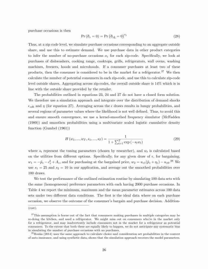
purchase occasions is then

Pr (ðz = 0) = Pr(ðzk = 0

)oz (28)

Thus, at a zip code level, we simulate purchase occasions corresponding to an aggregate outside

share, and use this to estimate demand. We use purchase data in other product categories

to infer the number of no-purchase occasions oz for each zip-code. Specifically, we look at

purchases of dishwashers, cooking range, cooktops, grills, refrigerators, wall ovens, washing

machines, freezers, hoods and microhoods. If a consumer purchases at least two of these

products, then the consumer is considered to be in the market for a refrigerator.37 We then

calculate the number of potential consumers in each zip-code, and use this to calculate zip-code

level outside shares. Aggregating across zip-codes, the overall outside share is 14% which is in

line with the outside share provided by the retailer.

The probabilities outlined in equations 23, 24 and 27 do not have a closed form solution.

We therefore use a simulation approach and integrate over the distribution of demand shocks

εzdk and η (for equation 27). Averaging across the ε draws results in lumpy probabilities, and

several regions of parameter values where the likelihood is not well defined. Thus, to avoid this

and ensure smooth convergence, we use a kernel-smoothed frequency simulator (McFadden

(1989)) and smoothen probabilities using a multivariate scaled logistic cumulative density

function (Gumbel (1961))

H (w1, ..., wT , s1, ..., sT ) =1

1 +∑T

t=1 exp (−stwt)(29)

where st represent the tuning parameters (chosen by researcher), and wt is calculated based

on the utilities from different options. Specifically, for any given draw of ε, for bargaining,

w1 = −pz − cbz +Az, and for purchasing at the bargained price, w2 = uz1(pz + ηz)− uz0.38 We

use s1 = 25 and s2 = 10 in our application, and average out the smoothed probabilities over

100 draws.

We test the performance of the outlined estimation routine by simulating 100 data sets with

the same (homogeneous) preference parameters with each having 2000 purchase occasions. In

Table 4 we report the minimum, maximum and the mean parameter estimates across 100 data

sets under two different data conditions. The first is the ideal data where on each purchase

occasion, we observe the outcome of the consumer’s bargain and purchase decision. Addition-

(cost).

37This assumption is borne out of the fact that consumers making purchases in multiple categories may bere-doing the kitchen, and need a refrigerator. We might miss out on consumers who’re in the market onlyfor a refrigerator, and may inadvertently include consumers not in the market for a refrigerator as potentialconsumers. To the extent that both these are equally likely to happen, we do not anticipate any systematic biasin simulating the number of purchase occasions with no purchases.

38Honka (2014) uses the same approach to calculate choice and consideration set probabilities in the contextof auto insurance, and using synthetic data, shows that the simulation approach recovers the model parameters.

26

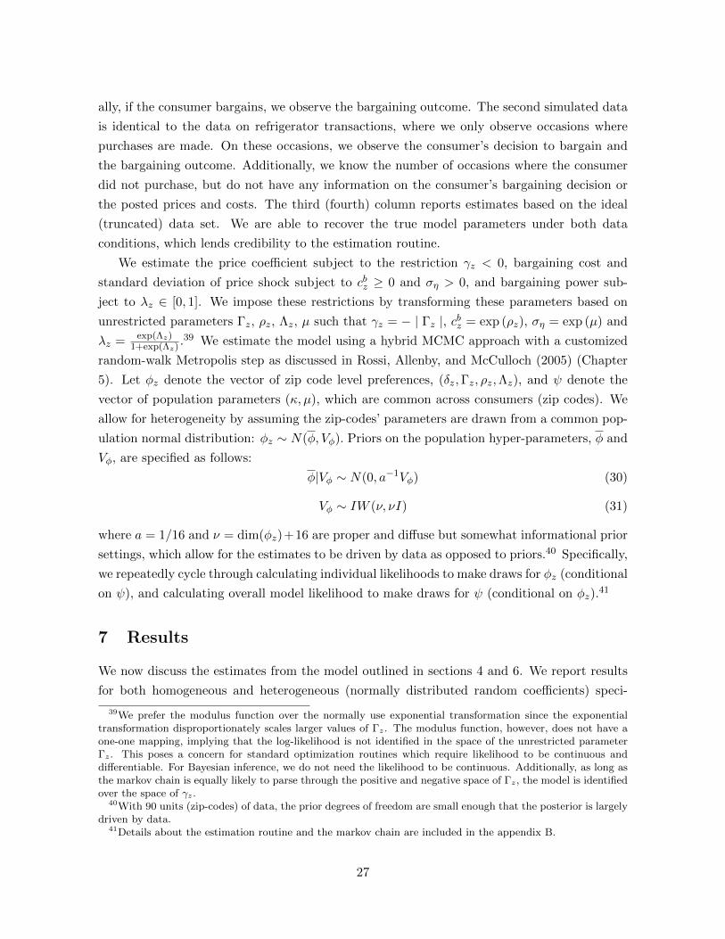
ally, if the consumer bargains, we observe the bargaining outcome. The second simulated data

is identical to the data on refrigerator transactions, where we only observe occasions where

purchases are made. On these occasions, we observe the consumer’s decision to bargain and

the bargaining outcome. Additionally, we know the number of occasions where the consumer

did not purchase, but do not have any information on the consumer’s bargaining decision or

the posted prices and costs. The third (fourth) column reports estimates based on the ideal

(truncated) data set. We are able to recover the true model parameters under both data

conditions, which lends credibility to the estimation routine.

We estimate the price coefficient subject to the restriction γz < 0, bargaining cost and

standard deviation of price shock subject to cbz ≥ 0 and ση > 0, and bargaining power sub-

ject to λz ∈ [0, 1]. We impose these restrictions by transforming these parameters based on

unrestricted parameters Γz, ρz, Λz, µ such that γz = − | Γz |, cbz = exp (ρz), ση = exp (µ) and

λz = exp(Λz)1+exp(Λz) .39 We estimate the model using a hybrid MCMC approach with a customized

random-walk Metropolis step as discussed in Rossi, Allenby, and McCulloch (2005) (Chapter

5). Let φz denote the vector of zip code level preferences, (δz,Γz, ρz,Λz), and ψ denote the

vector of population parameters (κ, µ), which are common across consumers (zip codes). We

allow for heterogeneity by assuming the zip-codes’ parameters are drawn from a common pop-

ulation normal distribution: φz ∼ N(φ, Vφ). Priors on the population hyper-parameters, φ and

Vφ, are specified as follows:

φ|Vφ ∼ N(0, a−1Vφ) (30)

Vφ ∼ IW (ν, νI) (31)

where a = 1/16 and ν = dim(φz)+16 are proper and diffuse but somewhat informational prior

settings, which allow for the estimates to be driven by data as opposed to priors.40 Specifically,

we repeatedly cycle through calculating individual likelihoods to make draws for φz (conditional

on ψ), and calculating overall model likelihood to make draws for ψ (conditional on φz).41

7 Results

We now discuss the estimates from the model outlined in sections 4 and 6. We report results

for both homogeneous and heterogeneous (normally distributed random coefficients) speci-

39We prefer the modulus function over the normally use exponential transformation since the exponentialtransformation disproportionately scales larger values of Γz. The modulus function, however, does not have aone-one mapping, implying that the log-likelihood is not identified in the space of the unrestricted parameterΓz. This poses a concern for standard optimization routines which require likelihood to be continuous anddifferentiable. For Bayesian inference, we do not need the likelihood to be continuous. Additionally, as long asthe markov chain is equally likely to parse through the positive and negative space of Γz, the model is identifiedover the space of γz.

40With 90 units (zip-codes) of data, the prior degrees of freedom are small enough that the posterior is largelydriven by data.

41Details about the estimation routine and the markov chain are included in the appendix B.

27

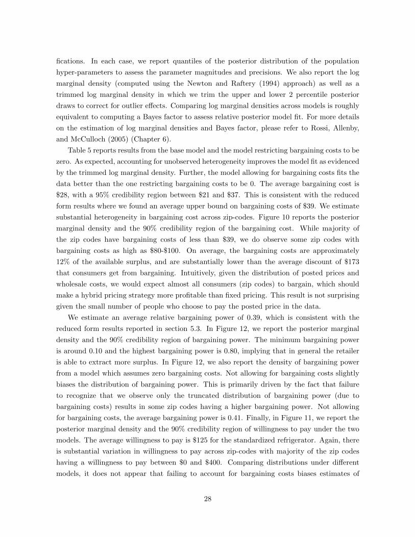
fications. In each case, we report quantiles of the posterior distribution of the population

hyper-parameters to assess the parameter magnitudes and precisions. We also report the log

marginal density (computed using the Newton and Raftery (1994) approach) as well as a

trimmed log marginal density in which we trim the upper and lower 2 percentile posterior

draws to correct for outlier effects. Comparing log marginal densities across models is roughly

equivalent to computing a Bayes factor to assess relative posterior model fit. For more details

on the estimation of log marginal densities and Bayes factor, please refer to Rossi, Allenby,

and McCulloch (2005) (Chapter 6).

Table 5 reports results from the base model and the model restricting bargaining costs to be

zero. As expected, accounting for unobserved heterogeneity improves the model fit as evidenced

by the trimmed log marginal density. Further, the model allowing for bargaining costs fits the

data better than the one restricting bargaining costs to be 0. The average bargaining cost is

$28, with a 95% credibility region between $21 and $37. This is consistent with the reduced

form results where we found an average upper bound on bargaining costs of $39. We estimate

substantial heterogeneity in bargaining cost across zip-codes. Figure 10 reports the posterior

marginal density and the 90% credibility region of the bargaining cost. While majority of

the zip codes have bargaining costs of less than $39, we do observe some zip codes with

bargaining costs as high as $80-$100. On average, the bargaining costs are approximately

12% of the available surplus, and are substantially lower than the average discount of $173

that consumers get from bargaining. Intuitively, given the distribution of posted prices and

wholesale costs, we would expect almost all consumers (zip codes) to bargain, which should

make a hybrid pricing strategy more profitable than fixed pricing. This result is not surprising

given the small number of people who choose to pay the posted price in the data.

We estimate an average relative bargaining power of 0.39, which is consistent with the

reduced form results reported in section 5.3. In Figure 12, we report the posterior marginal

density and the 90% credibility region of bargaining power. The minimum bargaining power

is around 0.10 and the highest bargaining power is 0.80, implying that in general the retailer

is able to extract more surplus. In Figure 12, we also report the density of bargaining power

from a model which assumes zero bargaining costs. Not allowing for bargaining costs slightly

biases the distribution of bargaining power. This is primarily driven by the fact that failure

to recognize that we observe only the truncated distribution of bargaining power (due to

bargaining costs) results in some zip codes having a higher bargaining power. Not allowing

for bargaining costs, the average bargaining power is 0.41. Finally, in Figure 11, we report the

posterior marginal density and the 90% credibility region of willingness to pay under the two

models. The average willingness to pay is $125 for the standardized refrigerator. Again, there

is substantial variation in willingness to pay across zip-codes with majority of the zip codes

having a willingness to pay between $0 and $400. Comparing distributions under different

models, it does not appear that failing to account for bargaining costs biases estimates of

28

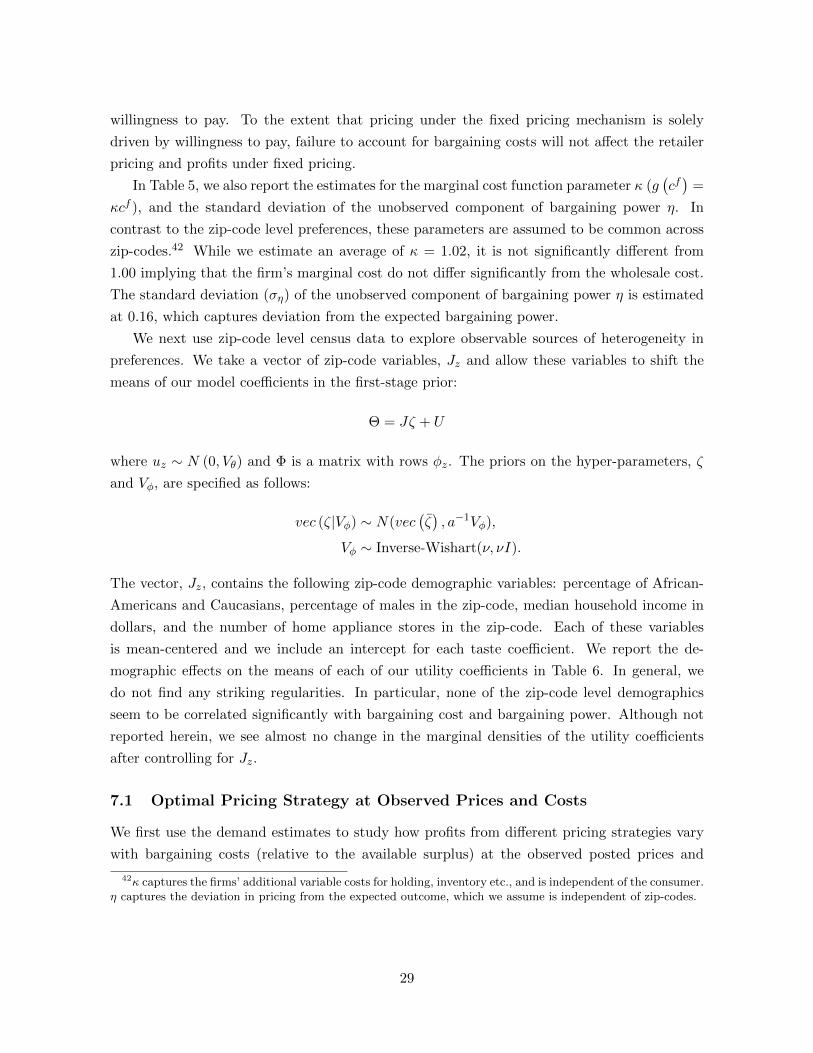
willingness to pay. To the extent that pricing under the fixed pricing mechanism is solely

driven by willingness to pay, failure to account for bargaining costs will not affect the retailer

pricing and profits under fixed pricing.

In Table 5, we also report the estimates for the marginal cost function parameter κ (g(cf)

=

κcf ), and the standard deviation of the unobserved component of bargaining power η. In

contrast to the zip-code level preferences, these parameters are assumed to be common across

zip-codes.42 While we estimate an average of κ = 1.02, it is not significantly different from

1.00 implying that the firm’s marginal cost do not differ significantly from the wholesale cost.

The standard deviation (ση) of the unobserved component of bargaining power η is estimated

at 0.16, which captures deviation from the expected bargaining power.

We next use zip-code level census data to explore observable sources of heterogeneity in

preferences. We take a vector of zip-code variables, Jz and allow these variables to shift the

means of our model coefficients in the first-stage prior:

Θ = Jζ + U

where uz ∼ N (0, Vθ) and Φ is a matrix with rows φz. The priors on the hyper-parameters, ζ

and Vφ, are specified as follows:

vec (ζ|Vφ) ∼ N(vec(ζ), a−1Vφ),

Vφ ∼ Inverse-Wishart(ν, νI).

The vector, Jz, contains the following zip-code demographic variables: percentage of African-

Americans and Caucasians, percentage of males in the zip-code, median household income in

dollars, and the number of home appliance stores in the zip-code. Each of these variables

is mean-centered and we include an intercept for each taste coefficient. We report the de-

mographic effects on the means of each of our utility coefficients in Table 6. In general, we

do not find any striking regularities. In particular, none of the zip-code level demographics

seem to be correlated significantly with bargaining cost and bargaining power. Although not

reported herein, we see almost no change in the marginal densities of the utility coefficients

after controlling for Jz.

7.1 Optimal Pricing Strategy at Observed Prices and Costs

We first use the demand estimates to study how profits from different pricing strategies vary

with bargaining costs (relative to the available surplus) at the observed posted prices and

42κ captures the firms’ additional variable costs for holding, inventory etc., and is independent of the consumer.η captures the deviation in pricing from the expected outcome, which we assume is independent of zip-codes.

29

wholesale costs.43 To do this, we simulate 200 consumers from multivariate distribution of

preferences and calculate retailer profits under hybrid pricing and fixed pricing at each com-

bination of posted price and wholesale cost. In the data, we observe 728 unique price-cost

combinations. In Figure 13, we plot the average bargaining cost ($28) divided by the differ-

ence between the observed posted price and the wholesale cost on the X-axis, and the difference

in profit between the hybrid pricing and the fixed pricing on the Y-axis.

Consistent with the bottom panel of Figure 3, we find that when bargaining costs are small

relative to the available surplus, hybrid pricing strategy (which allows for bargaining) is more

profitable than fixed pricing. When bargaining costs are more than 8% of the available surplus,

selling refrigerators at fixed pricing is more profitable for the retailer. Again, in line with the

simulation results, relative profits initially decrease and then increase as relative bargaining

costs increase. When bargaining costs are almost equal to the surplus, consumers do not have

an incentive to bargain, and thus, profits from hybrid and fixed pricing are the same (profit

difference is zero).

7.2 Optimal Prices and Bargaining Costs

The analysis in the previous section is insightful but is based on observed prices and costs. In

contrast, we now calculate the profit maximizing prices under alternate strategies and evaluate

(1) whether fixed pricing or hybrid pricing is more profitable for the retailer (at optimal prices),

and (2) how changes in retailers’ wholesale cost affect the optimal pricing strategy. The optimal

posted price under hybrid pricing solves

π∗ (p) = arg maxp

∫ ∫{∫ (

pi − κcf)

Pr (pi < p ∩ ui1 (pi) > ui0 | φz) dη

+(p− κcf

)Pr (pi = p ∩ ui1 (p) > ui0 | φz)}dFφzdε (32)

where Pr (pi < p ∩ ui1 (pi) > ui0 | φz) is the probability that any consumer from zip-code z

purchases at a bargained price , and Pr (pi = p ∩ ui1 (p) > ui0 | φz), is the probability that the

consumer purchases at the posted price. Similarly, the optimal price under fixed pricing solves

π∗ (p) = arg maxp

(p− κcf

)∫Pr (ui1 ≥ ui0 | δz, γz) dF(δz ,γz) (33)

where F(δz ,γz) is the joint distribution of δz and γz. For any assumed wholesale cost cf , we

calculate the optimal posted prices satisfying equations 32 and 33 by simulating from the

distributions of ε and η (equation 33 has a closed form solution). We repeat this exercise for

43Not accounting for consumers’ and retailer’s disagreement pay-offs may bias pricing in the counterfactualanalysis. However, to the extent that these do not bias pricing in the same direction, and may offset each other,their impact on firm pricing is ambiguous.

30

different values of cf , and in Figure 14, plot the optimal profits corresponding to these prices.44

Additionally, we report optimal profits based on the model which restricts bargaining costs to

be zero.

Recall that we are interested in studying how changes in bargaining cost (relative to the

available surplus) affect the optimal pricing strategy. Note that changing wholesale costs

(keeping bargaining costs fixed) changes the surplus relative to bargaining costs, and is similar

to changing bargaining costs in how it affects profits under bargaining strategy.45 This is driven

by the fact that changes in either of these costs makes consumers switch from bargaining to

paying posted prices, and vice versa. In contrast, under fixed pricing and in a model with

zero bargaining costs, consumers do not face any trade-off between buying at posted prices or

bargaining. Thus, while changes in bargaining cost do not affect profits under fixed pricing

and in a model with zero bargaining costs, increasing wholesale costs increase prices and affect

profits under fixed pricing (in a model with zero bargaining costs).

We first focus on the optimal profits under hybrid strategy based on estimates with non-zero

bargaining costs. Recall that in our data, the posted and transacted prices, and the wholesale

costs are computed based on the residuals from the quality adjusted price regressions. Thus,

the average wholesale cost observed in our data is −2.5, for which it is optimal for the retailer to

allow consumers to bargain. This is driven by the fact that bargaining costs are substantially

low compared to the potential gains from trade, and hence, all consumers bargain. As we

discuss in section 3.2, when most consumers bargain, the retailer extracts more profit by price

discriminating based on bargaining power.

As wholesale costs increase, the available surplus reduces and consumers are more likely to

pay posted prices or not purchase. The losses from consumers leaving the market offset the

gains from those paying posted prices, resulting in lower profits under bargaining as wholesale

costs increase. For fixed pricing and the model with zero bargaining costs, increasing wholesale

costs reduces retailer mark-up and profits. We reiterate that while increasing bargaining costs

will reduce firm profits under bargaining, they will not affect profits under fixed pricing and a

model with zero bargaining costs. Thus, Figure 14 redrawn with bargaining costs on the X-axis

will have horizontal lines for profits under fixed pricing and a model with zero bargaining costs.

As wholesale costs increase, fixed pricing becomes more attractive relative to a bargaining

mechanism for costs greater than around 4. Premium products are likely to have higher costs,

all else equal. Thus, if a retailer carries these premium products, the analysis implies that it

is more profitable for the retailer to have fixed pricing. This is consistent with Huang (2012),

who finds that vertically differentiated dealers are more likely to employ fixed pricing. Not

accounting for bargaining costs does not substantially affect the retailer’s profits. This is due

44Since posted prices are optimized over, plotting optimal profits with respect to the relative bargaining costcan be misleading. Thus, we plot the optimal profits relative to the retailer wholesale cost.

45This implicitly assumes that any changes in wholesale costs are not completely offset by correspondingchanges in posted prices.

31

to the fact that the estimated bargaining costs are relatively small, and that not allowing for

bargaining costs does not bias the distribution of willingness to pay. Failure to account for

bargaining costs do not affect optimal pricing in the current application, but may provide

misleading pricing implications in applications where bargaining costs are higher.

8 Discussion and Conclusion

This paper contributes to the empirical literature on bargaining, and quantifies and studies

the role of consumers’ bargaining costs in retailers’ optimal pricing strategy. We provide con-

sumers’ psychological bargaining costs as a possible explanation for why we observe bargaining

in some contexts and not in others. We show how these fixed bargaining costs can be identi-

fied based on transaction data, and use individual-level data on purchases of refrigerators to

estimate bargaining costs. In comparison to the previous literature, our ability to observe the

posted prices, and consumers purchasing at these prices is key to identification of bargaining

costs. We find that on average, consumers have a bargaining cost of $28, but there exists sub-

stantial heterogeneity in bargaining costs. Additionally, consumers on average, have a relative

bargaining power of 0.39, which implies that the retailer is more adept at bargaining.

Accounting for and estimating bargaining costs has important managerial implications.

First, estimation of bargaining costs provides unbiased measures of consumers’ willingness to

pay and retailers’ marginal costs. This allows the researcher to compare profits under fixed

pricing and under a bargaining strategy. For retailer wholesale costs commonly observed in

the data, it is more profitable for the retailer to allow consumers to bargain. As the wholesale

costs increase, bargaining becomes less attractive to consumers and it is more profitable for

the retailer to sell at posted prices. Thus, the retailer should engage in a bargaining strategy if

the consumers’ bargaining costs are relatively low compared to the potential surplus to be split

between the consumer and the retailer. Second, failure to account for bargaining costs may

provide biased estimates of bargaining power and retailer’s marginal cost, which could have

biased pricing implications. While we do not find evidence for this using data on transactions

for refrigerators; understandably, assuming zero bargaining costs will bias pricing more when

bargaining costs are higher.

Several directions exist for future research based on the findings herein. First, in this

paper, we assume that the retailer does not incur any bargaining costs. However, to the extent

that retailer bargaining costs might not be trivial and may affect optimal policy, a potential

extension would to quantify the retailer’s bargaining costs. Second, in this paper, we only

observe data on purchases, and have access to cross-sectional data. This requires us to make

some restrictive assumptions about heterogeneity. A possible extension would be to get access

to panel data, either in the business-to-business or in the business-to-consumer context, and

estimate a more flexible model.

32

References

Arnold, M. A., and S. A. Lippman (1998): “Posted PRices Versus Bargaining in Markets

with Asymmetric Information,” Economic Inquiry, 36, 450–457.

Bester, H. (1993): “Bargaining versus Price Competition in Markets with Quality Uncer-

tainty,” The American Economic Review, 83(1), 278–288.

Chen, Y., and R. W. Rosenthal (1996): “On the Use of Ceiling-Price as Commitments by

Monopolists,” The RAND Journal of Economics, 27(2), 207–220.

Chen, Y., S. Yang, and Y. Zhao (2008): “A Simultaneous Model of Consumer Brand

Choice and Negotiated Price,” Management Science, 54(3), 538–549.

Crawford, G. S., and A. Yurukoglu (2012): “The Welfare Effects of Bundling in Multi-

channel Television Markets,” American Economic Review, 102(2), 634–685.

Cui, T. H., P. Mallucci, and Z. J. Zhang (2014): “Competitive Implications of Haggling,”

manuscript.

Desai, P. S., and D. Purohit (2004): “”Let Me Talk to My Manager”:Haggling in a Com-

petetive Environment,” Marketing Science, 23(2), 219–233.

Draganska, M., D. Klapper, and S. B. Villas-Boas (2009): “A Larger Slice or a Larger

Pie? An Empirical Investigation of Bargaining Power in the Distribution Channel,” Mar-

keting Sci, 29 (1), 57–74.

Gill, D., and J. Thanassoulis (2013): “Competition in Posted Prices with Stochastic

Discounts,” Oxford Department of Economics Discussion Paper 682.

Gowrisankaran, G., A. Nevo, and R. Town (2014): “Mergers When Prices are Negoti-

ated: Evidence from the Hospital Industry,” American Economic Review, forthcoming.

Grennan, M. (2013): “Price Discrimination and Bargaining: Empirical Evidence from Med-

ical Devices,” American Economic Review, 103(1), 145–177.

Gumbel, E. J. (1961): “Bivariate Logistic Distributions,” Journal of the American Statistical

Association, Vol. 56, 335–349.

Honka, E. (2014): “Quantifying Search and Switching Costs in the U.S. Auto Insurance

Industry,” RAND Journal of Economics, forthcoming.

Hotz, V. J., and R. A. Miller (1993): “Conditional Choice Probabilities and the Estimation

of Dynamic Models,” Review of Economic Studies, 60(3), 497–529.

33

Huang, G. (2012): “Posted Price and Haggling in the Used Car Market,” manuscript.

Keniston, D. E. (2011): “Bargaining and Welfare: A Dynamic Structural Analysis of the

Autorickshaw Market,” manuscript.

Larsen, B. (2014): “The Efficiency of Real-World Bargaining: Evidence from Wholesale

Used-Auto Auctions,” manuscript.

McFadden, D. (1989): “A Method of Simulated Moments for Estimation of Discrete Response

Models without Numerical Integration,” Econometrica, Vol. 57, 995–1026.

Newton, M. A., and A. E. Raftery (1994): “Approximate Bayesian Inference with the

Weighted Likelihood Bootstrap,” Journal of the Royal Statistical Society. Series B (Method-

ological), Vol. 56, No. 1, 3–48.

Perry, M. (1986): “An Example of Price Formation in Bilateral Situations: A Bargaining

Model with Incomplete,” Econometrica, Vol. 54, No. 2, 313–321.

Rossi, P. E., G. M. Allenby, and R. McCulloch (2005): Bayesian Statistics and Mar-

keting. Wiley Series in Probability and Statistics.

Scott-Morton, F., J. Silva-Risso, and F. Zettelmeyer (2011): “What matters in a

price negotiation: Evidence from the U.S. auto retailing industry,” Quantitative Marketing

and Economics, 9, 365–402.

Wang, R. (1995): “Bargaining versus posted-price selling,” European Economic Review, 39,

1747–1764.

Zeng, X., S. Dasgupta, and C. B. Weinberg (2007): “Effects of a ”No-haggle” Internet

Channel on Marketing Strategies,” manuscript.

34

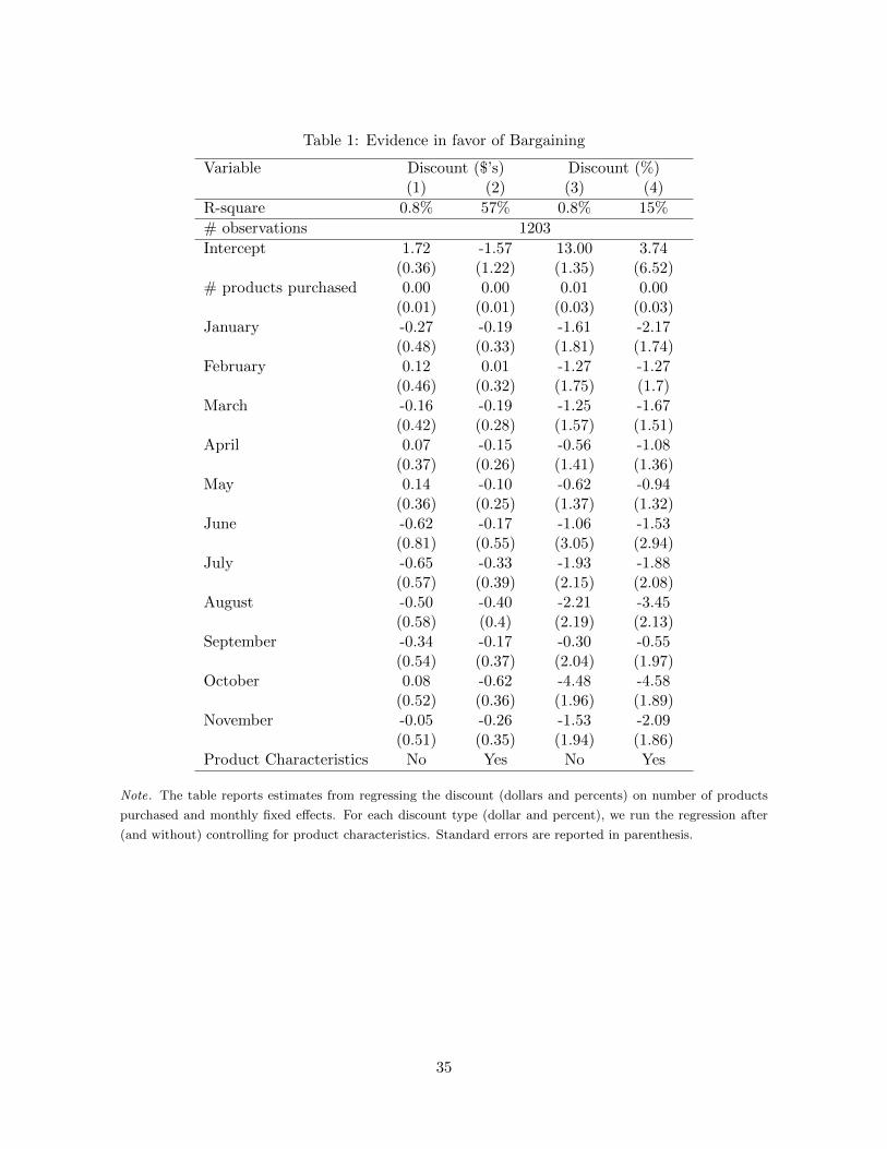
Table 1: Evidence in favor of Bargaining

Variable Discount ($’s) Discount (%)(1) (2) (3) (4)

R-square 0.8% 57% 0.8% 15%

# observations 1203

Intercept 1.72(0.36)

-1.57(1.22)

13.00(1.35)

3.74(6.52)

# products purchased 0.00(0.01)

0.00(0.01)

0.01(0.03)

0.00(0.03)

January -0.27(0.48)

-0.19(0.33)

-1.61(1.81)

-2.17(1.74)

February 0.12(0.46)

0.01(0.32)

-1.27(1.75)

-1.27(1.7)

March -0.16(0.42)

-0.19(0.28)

-1.25(1.57)

-1.67(1.51)

April 0.07(0.37)

-0.15(0.26)

-0.56(1.41)

-1.08(1.36)

May 0.14(0.36)

-0.10(0.25)

-0.62(1.37)

-0.94(1.32)

June -0.62(0.81)

-0.17(0.55)

-1.06(3.05)

-1.53(2.94)

July -0.65(0.57)

-0.33(0.39)

-1.93(2.15)

-1.88(2.08)

August -0.50(0.58)

-0.40(0.4)

-2.21(2.19)

-3.45(2.13)

September -0.34(0.54)

-0.17(0.37)

-0.30(2.04)

-0.55(1.97)

October 0.08(0.52)

-0.62(0.36)

-4.48(1.96)

-4.58(1.89)

November -0.05(0.51)

-0.26(0.35)

-1.53(1.94)

-2.09(1.86)

Product Characteristics No Yes No Yes

Note. The table reports estimates from regressing the discount (dollars and percents) on number of products

purchased and monthly fixed effects. For each discount type (dollar and percent), we run the regression after

(and without) controlling for product characteristics. Standard errors are reported in parenthesis.

35

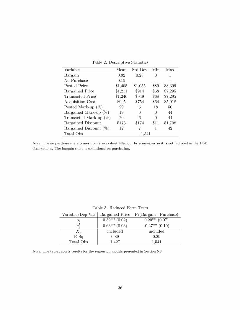
Table 2: Descriptive Statistics

Variable Mean Std Dev Min Max

Bargain 0.92 0.28 0 1No Purchase 0.15 - - -Posted Price $1,405 $1,055 $89 $8,399Bargained Price $1,211 $914 $68 $7,295Transacted Price $1,246 $949 $68 $7,295Acquisition Cost $995 $754 $64 $5,918Posted Mark-up (%) 29 5 18 50Bargained Mark-up (%) 19 6 0 44Transacted Mark-up (%) 20 6 0 44Bargained Discount $173 $174 $11 $1,708Bargained Discount (%) 12 7 1 42

Total Obs 1,541

Note. The no purchase share comes from a worksheet filled out by a manager so it is not included in the 1,541

observations. The bargain share is conditional on purchasing.

Table 3: Reduced Form Tests

Variable/Dep Var Bargained Price Pr(Bargain | Purchase)

pk 0.39** (0.02) 0.20** (0.07)

cfk 0.63** (0.03) -0.27** (0.10)

Xk included includedR-Sq 0.89 0.29

Total Obs 1,427 1,541

Note. The table reports results for the regression models presented in Section 5.3.

36

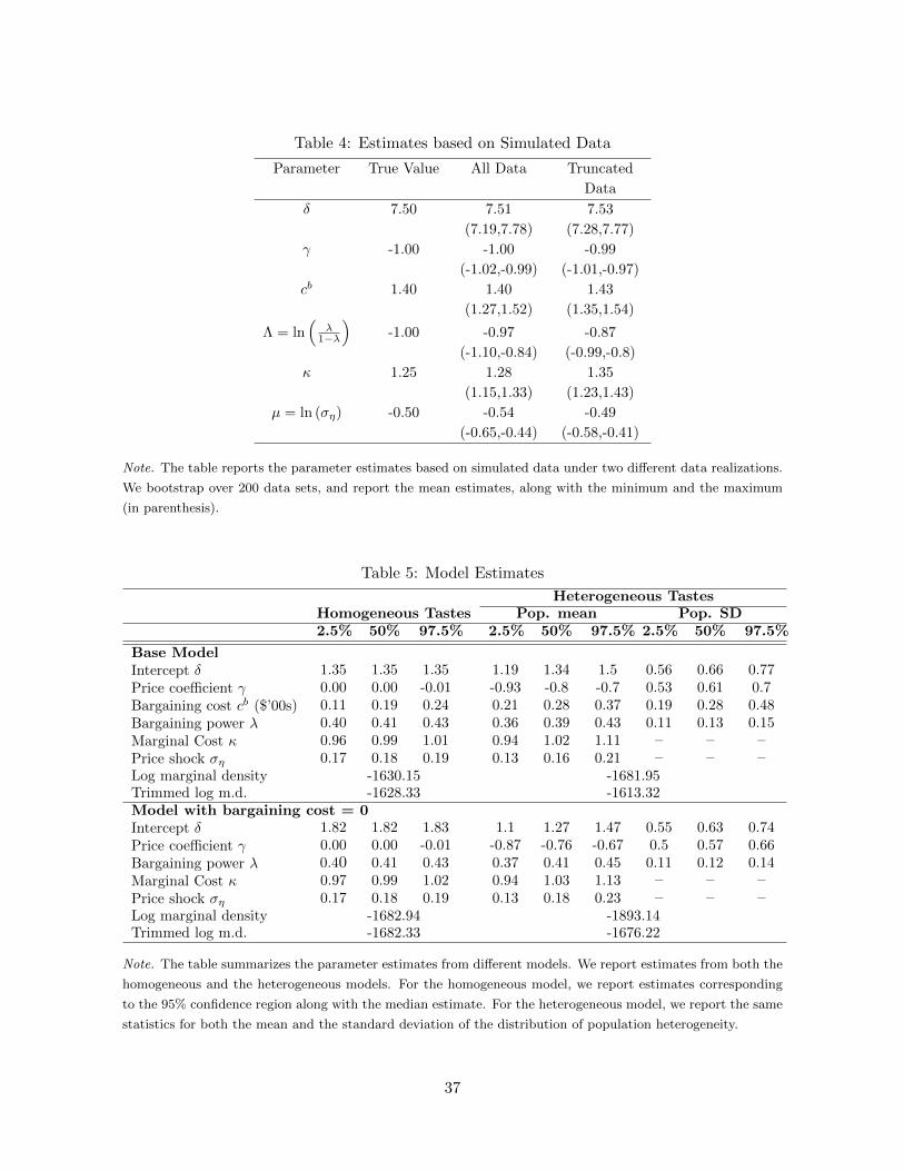
Table 4: Estimates based on Simulated Data

Parameter True Value All Data Truncated

Data

δ 7.50 7.51

(7.19,7.78)

7.53

(7.28,7.77)

γ -1.00 -1.00

(-1.02,-0.99)

-0.99

(-1.01,-0.97)

cb 1.40 1.40

(1.27,1.52)

1.43

(1.35,1.54)

Λ = ln(

λ1−λ

)-1.00 -0.97

(-1.10,-0.84)

-0.87

(-0.99,-0.8)

κ 1.25 1.28

(1.15,1.33)

1.35

(1.23,1.43)

µ = ln (ση) -0.50 -0.54

(-0.65,-0.44)

-0.49

(-0.58,-0.41)

Note. The table reports the parameter estimates based on simulated data under two different data realizations.

We bootstrap over 200 data sets, and report the mean estimates, along with the minimum and the maximum

(in parenthesis).

Table 5: Model Estimates

Heterogeneous TastesHomogeneous Tastes Pop. mean Pop. SD2.5% 50% 97.5% 2.5% 50% 97.5% 2.5% 50% 97.5%

Base ModelIntercept δ 1.35 1.35 1.35 1.19 1.34 1.5 0.56 0.66 0.77Price coefficient γ 0.00 0.00 -0.01 -0.93 -0.8 -0.7 0.53 0.61 0.7Bargaining cost cb ($’00s) 0.11 0.19 0.24 0.21 0.28 0.37 0.19 0.28 0.48Bargaining power λ 0.40 0.41 0.43 0.36 0.39 0.43 0.11 0.13 0.15Marginal Cost κ 0.96 0.99 1.01 0.94 1.02 1.11 – – –Price shock ση 0.17 0.18 0.19 0.13 0.16 0.21 – – –Log marginal density -1630.15 -1681.95Trimmed log m.d. -1628.33 -1613.32Model with bargaining cost = 0Intercept δ 1.82 1.82 1.83 1.1 1.27 1.47 0.55 0.63 0.74Price coefficient γ 0.00 0.00 -0.01 -0.87 -0.76 -0.67 0.5 0.57 0.66Bargaining power λ 0.40 0.41 0.43 0.37 0.41 0.45 0.11 0.12 0.14Marginal Cost κ 0.97 0.99 1.02 0.94 1.03 1.13 – – –Price shock ση 0.17 0.18 0.19 0.13 0.18 0.23 – – –Log marginal density -1682.94 -1893.14Trimmed log m.d. -1682.33 -1676.22

Note. The table summarizes the parameter estimates from different models. We report estimates from both the

homogeneous and the heterogeneous models. For the homogeneous model, we report estimates corresponding

to the 95% confidence region along with the median estimate. For the heterogeneous model, we report the same

statistics for both the mean and the standard deviation of the distribution of population heterogeneity.

37

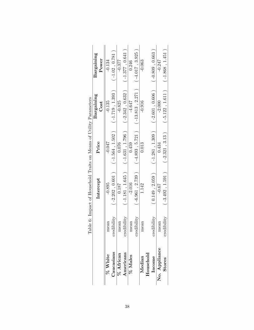
Tab

le6:

Imp

act

ofH

ouse

hol

dT

rait

son

Mea

ns

ofU

tili

tyP

aram

eter

s

Inte

rcep

tP

rice

Barg

ain

ing

Cost

Barg

ain

ing

Pow

er

%W

hit

em

ean

-0.8

95-0

.047

-0.1

35-0

.134

Cau

casi

an

scr

edib

ilit

y(

-2.2

02,

0.60

1)

(-1

.564

,1.

502

)(

-1.7

19,

1.39

3)

(-1

.02

,0.

781

)

%A

fric

an

mea

n0.

187

0.07

6-0

.825

-0.3

77A

meri

can

scr

edib

ilit

y(

-1.1

81,

1.64

5)

(-1

.631

,1.

796

)(

-2.3

42,

0.63

2)

(-1

.377

,0.

641

)

%M

ale

sm

ean

-2.0

160.

459

-4.6

470.

246

cred

ibil

ity

(-6

.961

,2.

739

)(

-4.8

93,

5.72

1)

(-1

3.81

3,

2.27

1)

(-4

.017

,3.

925

)

Med

ian

Hou

seh

old

mea

n1.

142

0.01

3-0

.916

-0.0

63

Incom

ecr

edib

ilit

y(

0.14

9,

2.05

9)

(-1

.281

,1.

309

)(

-2.6

01,

0.60

6)

(-0

.809

,0.

663

)

No.

Ap

plian

ce

mea

n-0

.67

0.43

4-2

.000

-0.2

47S

tore

scr

edib

ilit

y(

-3.4

92,

1.59

1)

(-2

.321

,3.

13)

(-5

.122

,1.

611

)(

-1.8

68,

1.45

1)

38

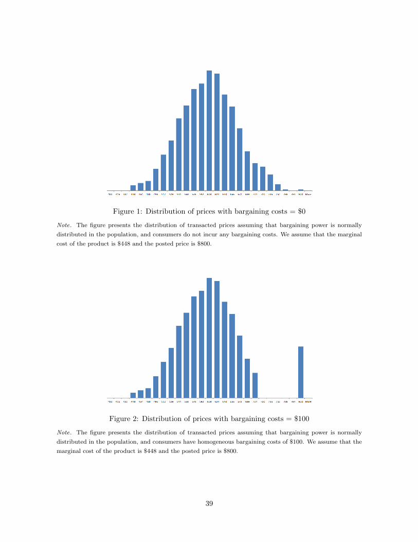
Figure 1: Distribution of prices with bargaining costs = $0

Note. The figure presents the distribution of transacted prices assuming that bargaining power is normally

distributed in the population, and consumers do not incur any bargaining costs. We assume that the marginal

cost of the product is $448 and the posted price is $800.

Figure 2: Distribution of prices with bargaining costs = $100

Note. The figure presents the distribution of transacted prices assuming that bargaining power is normally

distributed in the population, and consumers have homogeneous bargaining costs of $100. We assume that the

marginal cost of the product is $448 and the posted price is $800.

39

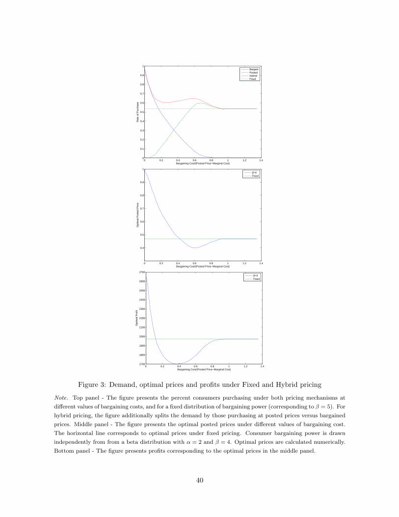
0 0.2 0.4 0.6 0.8 1 1.2 1.40

0.1

0.2

0.3

0.4

0.5

0.6

0.7

0.8

0.9

1

Bargaining Cost/(Posted Price−Marginal Cost)

Rat

e of

Pur

chas

e

BargainPostedHybridFixed

0 0.2 0.4 0.6 0.8 1 1.2 1.4

0.4

0.5

0.6

0.7

0.8

0.9

1

Bargaining Cost/(Posted Price−Marginal Cost)

Opt

imal

Pos

ted

Pric

e

β=4Fixed

0 0.2 0.4 0.6 0.8 1 1.2 1.41700

1800

1900

2000

2100

2200

2300

2400

2500

2600

2700

Bargaining Cost/(Posted Price−Marginal Cost)

Opt

imal

Pro

fit

β=4Fixed

Figure 3: Demand, optimal prices and profits under Fixed and Hybrid pricing

Note. Top panel - The figure presents the percent consumers purchasing under both pricing mechanisms at

different values of bargaining costs, and for a fixed distribution of bargaining power (corresponding to β = 5). For

hybrid pricing, the figure additionally splits the demand by those purchasing at posted prices versus bargained

prices. Middle panel - The figure presents the optimal posted prices under different values of bargaining cost.

The horizontal line corresponds to optimal prices under fixed pricing. Consumer bargaining power is drawn

independently from from a beta distribution with α = 2 and β = 4. Optimal prices are calculated numerically.

Bottom panel - The figure presents profits corresponding to the optimal prices in the middle panel.

40

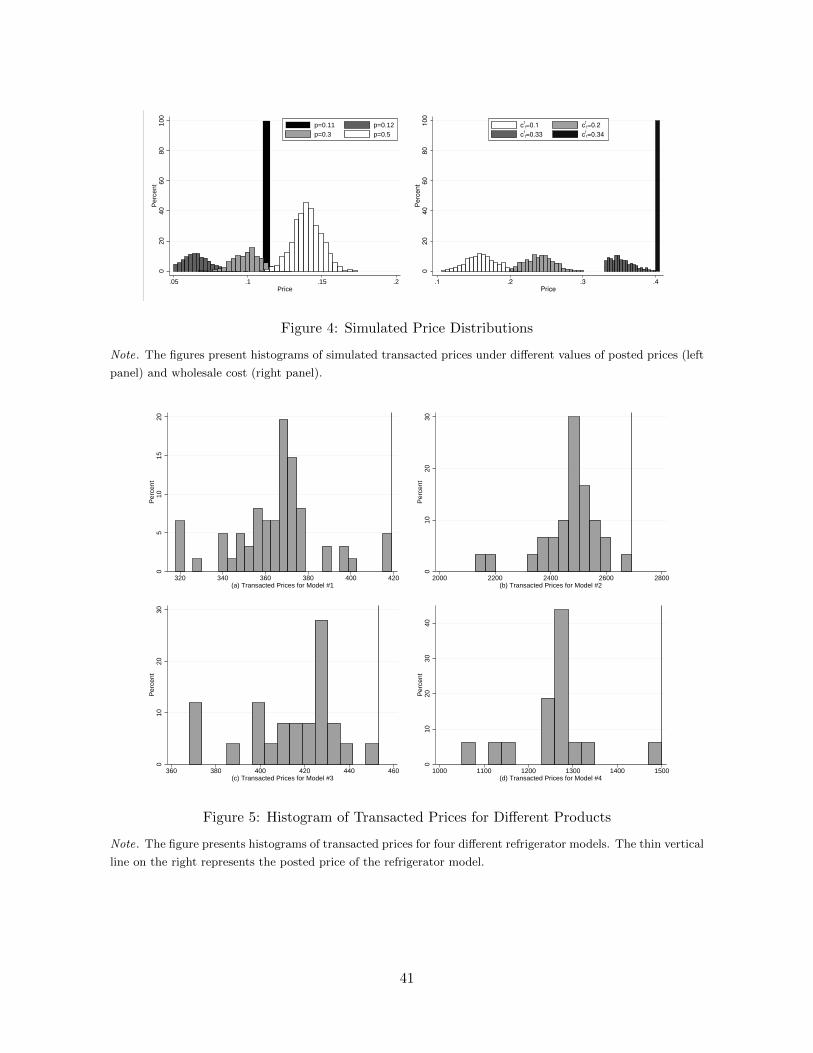
020

4060

8010

0P

erce

nt

.05 .1 .15 .2Price

p=0.11 p=0.12p=0.3 p=0.5

020

40

60

80

100

Perc

ent

.1 .2 .3 .4

Price

cf

t=0.1 cf

t=0.2

cf

t=0.33 cf

t=0.34

Figure 4: Simulated Price Distributions

Note. The figures present histograms of simulated transacted prices under different values of posted prices (left

panel) and wholesale cost (right panel).

05

1015

20P

erce

nt

320 340 360 380 400 420(a) Transacted Prices for Model #1

010

2030

Per

cent

2000 2200 2400 2600 2800(b) Transacted Prices for Model #2

010

2030

Per

cent

360 380 400 420 440 460(c) Transacted Prices for Model #3

010

2030

40P

erce

nt

1000 1100 1200 1300 1400 1500(d) Transacted Prices for Model #4

Figure 5: Histogram of Transacted Prices for Different Products

Note. The figure presents histograms of transacted prices for four different refrigerator models. The thin vertical

line on the right represents the posted price of the refrigerator model.

41

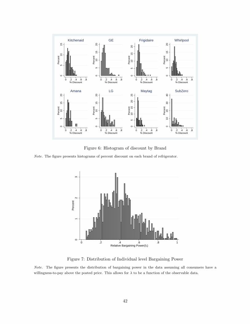
05

1015

Per

cent

0 .2 .4 .6 .8% Discount

Kitchenaid

05

1015

20P

erce

nt

0 .2 .4 .6 .8% Discount

GE

05

1015

20P

erce

nt

0 .2 .4 .6 .8% Discount

Frigidaire

05

1015

20P

erce

nt

0 .2 .4 .6 .8% Discount

Whirlpool

05

1015

20P

erce

nt

0 .2 .4 .6 .8% Discount

Amana

05

1015

20P

erce

nt

0 .2 .4 .6 .8% Discount

LG

05

1015

2025

Per

cent

0 .2 .4 .6 .8% Discount

Maytag

010

2030

40P

erce

nt

0 .2 .4 .6 .8% Discount

SubZero

Figure 6: Histogram of discount by Brand

Note. The figure presents histograms of percent discount on each brand of refrigerator.

01

23

Per

cent

0 .2 .4 .6 .8 1Relative Bargaining Power(λi)

Figure 7: Distribution of Individual level Bargaining Power

Note. The figure presents the distribution of bargaining power in the data assuming all consumers have a

willingness-to-pay above the posted price. This allows for λ to be a function of the observable data.

42

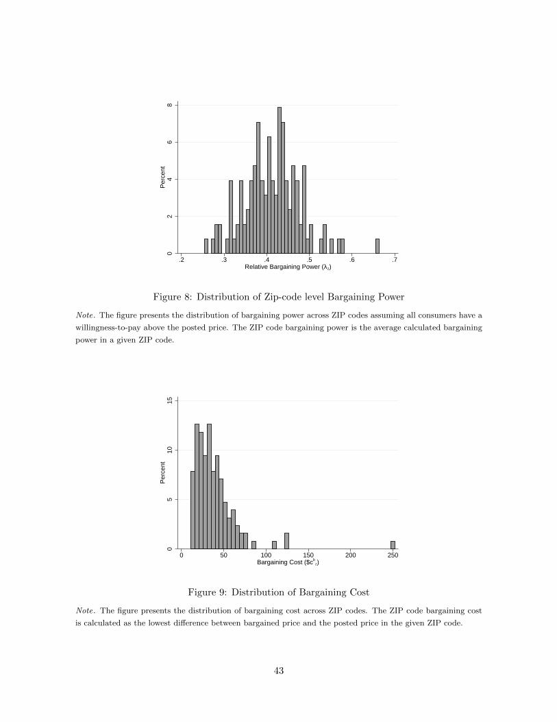
02

46

8P

erce

nt

.2 .3 .4 .5 .6 .7Relative Bargaining Power (λz)

Figure 8: Distribution of Zip-code level Bargaining Power

Note. The figure presents the distribution of bargaining power across ZIP codes assuming all consumers have a

willingness-to-pay above the posted price. The ZIP code bargaining power is the average calculated bargaining

power in a given ZIP code.

05

1015

Per

cent

0 50 100 150 200 250Bargaining Cost ($cb

z)

Figure 9: Distribution of Bargaining Cost

Note. The figure presents the distribution of bargaining cost across ZIP codes. The ZIP code bargaining cost

is calculated as the lowest difference between bargained price and the posted price in the given ZIP code.

43

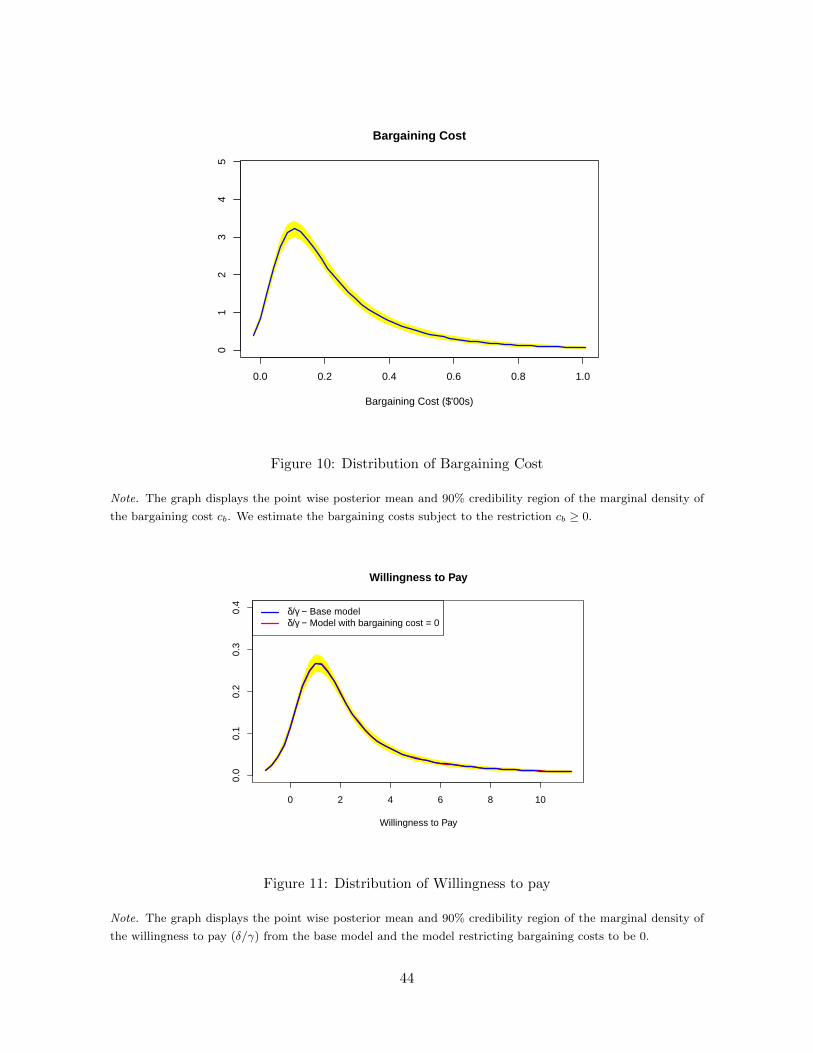
0.0 0.2 0.4 0.6 0.8 1.0

01

23

45

Bargaining Cost

Bargaining Cost ($'00s)

Figure 10: Distribution of Bargaining Cost

Note. The graph displays the point wise posterior mean and 90% credibility region of the marginal density of

the bargaining cost cb. We estimate the bargaining costs subject to the restriction cb ≥ 0.

0 2 4 6 8 10

0.0

0.1

0.2

0.3

0.4

Willingness to Pay

Willingness to Pay

δ/γ − Base modelδ/γ − Model with bargaining cost = 0

Figure 11: Distribution of Willingness to pay

Note. The graph displays the point wise posterior mean and 90% credibility region of the marginal density of

the willingness to pay (δ/γ) from the base model and the model restricting bargaining costs to be 0.

44

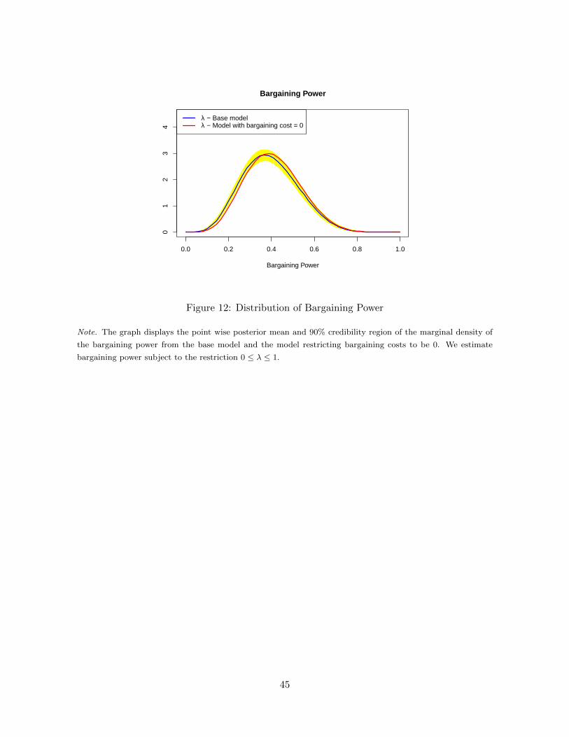
0.0 0.2 0.4 0.6 0.8 1.0

01

23

4

Bargaining Power

Bargaining Power

λ − Base modelλ − Model with bargaining cost = 0

Figure 12: Distribution of Bargaining Power

Note. The graph displays the point wise posterior mean and 90% credibility region of the marginal density of

the bargaining power from the base model and the model restricting bargaining costs to be 0. We estimate

bargaining power subject to the restriction 0 ≤ λ ≤ 1.

45

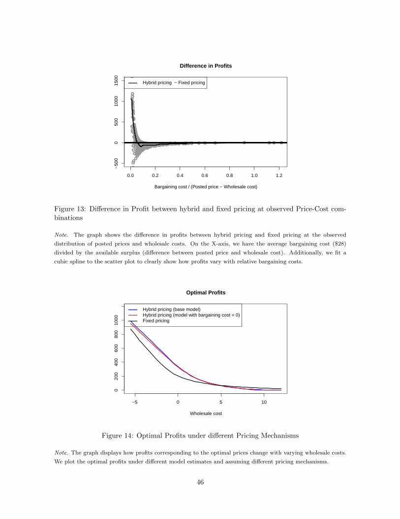
0.0 0.2 0.4 0.6 0.8 1.0 1.2

−50

00

500

1000

1500

Difference in Profits

Bargaining cost / (Posted price − Wholesale cost)

Hybrid pricing − Fixed pricing

●●

● ●

●

●

●●●

●●

●

●●●

●●

●

●

●

●

●●

●

●●

●

●

●

●

●●

● ●●

●

●

●

●

●

●●●

●●●

●

●

●

●

●●

●

●●

●●

● ●

●

●

●●

●

●●●

● ●●

●

●

●●

●●

●●●

●

●

●

●

●

●

●

●●

●● ●

●

●

●●

●

●

●●

●

●

● ●●

●

●

●

●

●●

●

●

●

●

●●

●●

●●●

●

●

●

●

●

●

●●

●

●

●

●

●●

●

●● ●

●

●●

●

●

● ●●●

●●

●

●

●●

●

●

●

●

●

●●●●●

●

●

●

●●● ●●●

●●

●●

●

●

●●●

●

●

●

●

●

●

●

●

●

●

●●●

●

●●

●●●

●

●● ●●●● ●

●

●

●

●

●

●

●

●●●

● ●●●●● ● ●

●

●●●

●

●●

●

●

●●

●●

●

●

●

●●●

●●

●●

● ●●● ●

●

●

●

●●

●●●

●

●

●

●●

●

●

●●

●

●●

●

●●

●●

●●

●●●

●

●●

●

●

●

●

●

●●

●●● ●

●

●●

●●

●

●

●

●

●

●

●

●

●●●

●

●

●

●

●

● ●●

●

● ●●● ●●

●●

●

●

●

●

●

●

●●

●●

●

●

●● ●●

●

●●●

●●

●

●

● ●

●

● ●●

●

●●

●● ●

●

●

●

●●

●●

●●

●

●

●

●

●

●●

●

●

●

●

●●

●

●●●

●

●●●

●

●● ●●

●

●

● ●●●

●

●

●●●

●●

● ●●●●●● ●● ●

●

●

●

● ● ●●● ●

●

●● ●

●

●●●●

●●●

●

●

●

●●●

●

● ●

●

●●●

●●

●

●

●

●●●

●

●●

●

●●

●

●

● ●●

●

●

●●

● ●●

●●

●

●

●

●

●

●●

●●

●

●●

●

●

●●●

●●

●

●

●●

●●

●

●

●●● ●

●

●

●

●

●●●

●●●

●

●

●

●●●

●

●

●

●

●●●

●●

●

●

●

●●

●

●

●

●●

● ●

●●

●

●●●

●●●

●●

●

●

●

●

●

●

●

●●

●

●● ●

●

●●

●●●

●

●

●

●

●

●

●●

●

●●

●

●● ●●●

●

●●

●

●

●

●

●

●

●

●

●

●

●●

●

●

●

●

●

●

●●

●●

●

●●

●

●●●

●

●

●●

●

●●

●

●

●

●●●●

●● ●●● ●

●

●●

●●● ● ● ●●

●

●

●●

●● ●●●

●

●●

●

●

●

●●●

●

●

● ●

●

●●

●

●

●

●

●

●

●●●

●

●

●

●

● ●●

●

●

● ●●

●

●●

●●

●

●

●●● ●

●●

●

●●

Figure 13: Difference in Profit between hybrid and fixed pricing at observed Price-Cost com-binations

Note. The graph shows the difference in profits between hybrid pricing and fixed pricing at the observed

distribution of posted prices and wholesale costs. On the X-axis, we have the average bargaining cost ($28)

divided by the available surplus (difference between posted price and wholesale cost). Additionally, we fit a

cubic spline to the scatter plot to clearly show how profits vary with relative bargaining costs.

−5 0 5 10

020

040

060

080

010

00

Optimal Profits

Wholesale cost

Hybrid pricing (base model) Hybrid pricing (model with bargaining cost = 0) Fixed pricing

Figure 14: Optimal Profits under different Pricing Mechanisms

Note. The graph displays how profits corresponding to the optimal prices change with varying wholesale costs.

We plot the optimal profits under different model estimates and assuming different pricing mechanisms.

46

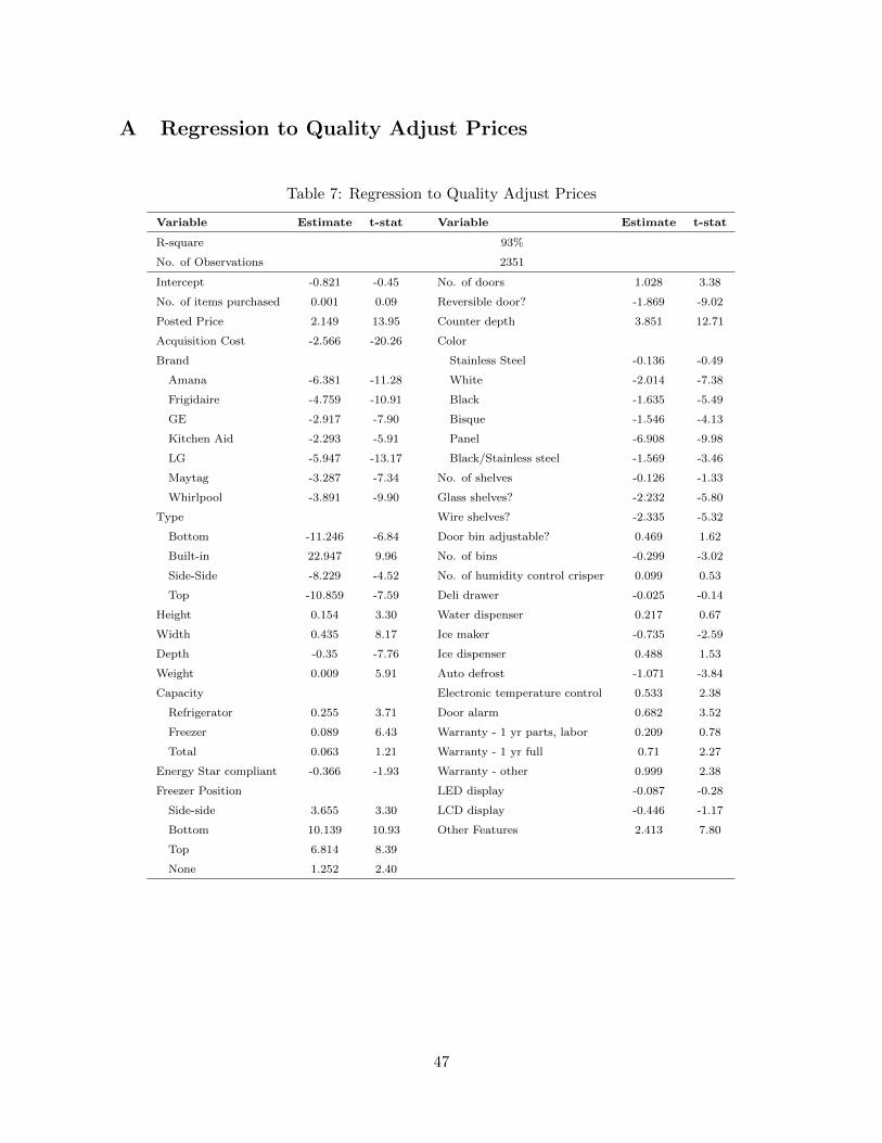
A Regression to Quality Adjust Prices

Table 7: Regression to Quality Adjust Prices

Variable Estimate t-stat Variable Estimate t-stat

R-square 93%

No. of Observations 2351

Intercept -0.821 -0.45 No. of doors 1.028 3.38

No. of items purchased 0.001 0.09 Reversible door? -1.869 -9.02

Posted Price 2.149 13.95 Counter depth 3.851 12.71

Acquisition Cost -2.566 -20.26 Color

Brand Stainless Steel -0.136 -0.49

Amana -6.381 -11.28 White -2.014 -7.38

Frigidaire -4.759 -10.91 Black -1.635 -5.49

GE -2.917 -7.90 Bisque -1.546 -4.13

Kitchen Aid -2.293 -5.91 Panel -6.908 -9.98

LG -5.947 -13.17 Black/Stainless steel -1.569 -3.46

Maytag -3.287 -7.34 No. of shelves -0.126 -1.33

Whirlpool -3.891 -9.90 Glass shelves? -2.232 -5.80

Type Wire shelves? -2.335 -5.32

Bottom -11.246 -6.84 Door bin adjustable? 0.469 1.62

Built-in 22.947 9.96 No. of bins -0.299 -3.02

Side-Side -8.229 -4.52 No. of humidity control crisper 0.099 0.53

Top -10.859 -7.59 Deli drawer -0.025 -0.14

Height 0.154 3.30 Water dispenser 0.217 0.67

Width 0.435 8.17 Ice maker -0.735 -2.59

Depth -0.35 -7.76 Ice dispenser 0.488 1.53

Weight 0.009 5.91 Auto defrost -1.071 -3.84

Capacity Electronic temperature control 0.533 2.38

Refrigerator 0.255 3.71 Door alarm 0.682 3.52

Freezer 0.089 6.43 Warranty - 1 yr parts, labor 0.209 0.78

Total 0.063 1.21 Warranty - 1 yr full 0.71 2.27

Energy Star compliant -0.366 -1.93 Warranty - other 0.999 2.38

Freezer Position LED display -0.087 -0.28

Side-side 3.655 3.30 LCD display -0.446 -1.17

Bottom 10.139 10.93 Other Features 2.413 7.80

Top 6.814 8.39

None 1.252 2.40

47

B Estimation Details and Markov Chain

As mentioned in section 6, φz ≡ (δz,Γz, ρz,Λz) is the vector of zip code level preferences, and

ψ ≡ (κ, µ) is the vector of population parameters. We allow for heterogeneity by assuming

the consumers’ parameters are drawn from a common population normal distribution: φz ∼N(φ, Vφ). Priors on the population hyper-parameters, φ and Vφ, are specified as φ|Vφ ∼N(0, a−1Vφ) and Vφ ∼ IW (ν, νI) where a = 1/16 and ν = dim(φz) + 16 are proper and diffuse

but somewhat informational prior settings, which allow for the estimates to be driven by data

as opposed to priors.

We assume normal priors for the parameters common across zip codes i.e. ψ ∼ N(ψ,A−1).

The markov chain is constructed as follows:

1. Draw φz | φ, Vφ, ψ

2. Draw φ, Vφ | φz, ψ

3. Draw ψ | φz, φ, Vφ

4. Repeat steps 1-3

C Competition and Retailer’s Disagreement Pay-off

Following the model outlined in section 4, let consumer i′s disagreement pay-off on purchase

occasion k also depend on a possible price pik available at some other store. Thus, equation 3

becomes

dcik =

0 ; wik < min {pk, pik}

wik −min {pk, pik} ; wik ≥ min {pk, pik}(34)

Further, let retailer’s disagreement pay-off equal drk. If the consumer bargains, the optimal

bargained price equals

pik = (1− λi)Aik + λi

[g(cfk

)+ drk

]+ ηik

(Aik − g

(cfk

))(35)

where Aik = min {wik, pk, pik} and wik = δi+ε1ik−ε0ik−γi . As before, let X be the support of x.

Assume the support X is large enough such that for any p′, an x′ ∈ X exists such that (i) p′

is the p-component of x′, (ii) min{δ+ε1−ε0−γ , p

}> p′ and (iii) p (x′) + cb < p′. Intuitively, this

implies that there exists a range of posted prices for which both, consumer’s willingness to pay

(accounting for the utility shocks) and the price available at another store are always greater

than the posted price, and the consumer chooses to bargain. Equation 18 can be rewritten as

p(x′)

= E (p) = (1− λ)p′ + λ[g(cfk

)+ drk

](36)

48

Thus, the expected transacted price is identified through repeated transactions at the same

posted price and wholesale cost. Let there be p′′ such that (i) p′′ is the p-component of x′′,

(ii)p′′ < p′, (iii) p (x′′) + cb < p′′ and (iv) drk is the same for x′ and x′′. The last assumption

(made in addition to the previous ones) implies that retailer’s disagreement pay-off does not

endogenously vary as the posted price changes. Computing the difference between the expected

price at x′ (equation 36) and x′′, we get

p(x′)− p

(x′′)

= (1− λ)(p′ − p′′

)(37)

=⇒ λ = 1− p (x′)− p (x′′)

(p′ − p′′)(38)

Thus, bargaining power is identified independent of bargaining cost, marginal cost function

g(cf), and the distribution of η even in the absence of knowledge about retailer’s disagreement

pay-off drk (subject to the assumption that retailer disagreement pay-offs do not vary with

posted price). Since the expected price is inferred from data, and does not require prior

knowledge of the retailer’s disagreement pay-off, bargaining costs are identified as before i.e.

they are the difference between the consumers’ reservation price and the expected price at

the threshold for which the consumer is indifferent between bargaining and paying the posted

price.

D Robustness Analysis

Quality Adjusted Prices

In the paper, we calculate quality adjusted prices by stacking posted prices, transacted prices,

and wholesale costs. We now quality adjust prices in two other ways and check robustness of

our estimates to these. Specifically, we just regress posted prices on product characteristics,

and quality adjust prices such that pr = p − ˆp, pri = pi − ˆp, and cfr = cf − ˆp, where pr, pri ,

and cfr are the residual posted prices, transacted prices, and wholesale costs. respectively.

Alternately, we regress wholesale costs on product characteristics, and quality adjust prices

accordingly. The estimates from these alternate models are reported in Table 8. The model

fits these alternate data slightly better but we do not find much qualitative differences in the

parameter estimates. Figures 15, 16, and 17 report the density of willingness to pay, bargaining

cost and bargaining power for the model estimated using the original quality adjusted prices,

and the two different sets of prices (outlined above). For the base data, we additionally shade

the 90% credibility region for the density of preferences. Based on the estimates and the density

plots, the preference estimates and pricing implications are not driven by how we quality adjust

prices.

49

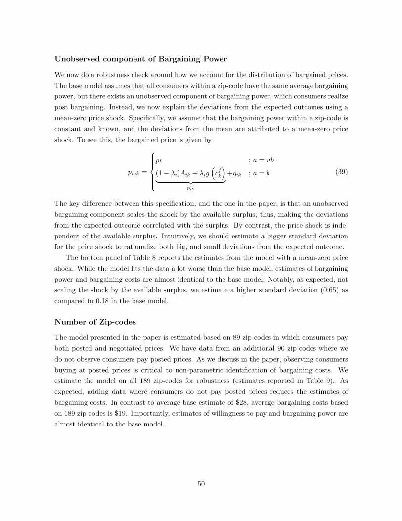
Unobserved component of Bargaining Power

We now do a robustness check around how we account for the distribution of bargained prices.

The base model assumes that all consumers within a zip-code have the same average bargaining

power, but there exists an unobserved component of bargaining power, which consumers realize

post bargaining. Instead, we now explain the deviations from the expected outcomes using a

mean-zero price shock. Specifically, we assume that the bargaining power within a zip-code is

constant and known, and the deviations from the mean are attributed to a mean-zero price

shock. To see this, the bargained price is given by

piak =

pk ; a = nb

(1− λi)Aik + λig(cfk

)︸ ︷︷ ︸

˜pik

+ηik ; a = b (39)

The key difference between this specification, and the one in the paper, is that an unobserved

bargaining component scales the shock by the available surplus; thus, making the deviations

from the expected outcome correlated with the surplus. By contrast, the price shock is inde-

pendent of the available surplus. Intuitively, we should estimate a bigger standard deviation

for the price shock to rationalize both big, and small deviations from the expected outcome.

The bottom panel of Table 8 reports the estimates from the model with a mean-zero price

shock. While the model fits the data a lot worse than the base model, estimates of bargaining

power and bargaining costs are almost identical to the base model. Notably, as expected, not

scaling the shock by the available surplus, we estimate a higher standard deviation (0.65) as

compared to 0.18 in the base model.

Number of Zip-codes

The model presented in the paper is estimated based on 89 zip-codes in which consumers pay

both posted and negotiated prices. We have data from an additional 90 zip-codes where we

do not observe consumers pay posted prices. As we discuss in the paper, observing consumers

buying at posted prices is critical to non-parametric identification of bargaining costs. We

estimate the model on all 189 zip-codes for robustness (estimates reported in Table 9). As

expected, adding data where consumers do not pay posted prices reduces the estimates of

bargaining costs. In contrast to average base estimate of $28, average bargaining costs based

on 189 zip-codes is $19. Importantly, estimates of willingness to pay and bargaining power are

almost identical to the base model.

50

Model Specification and Bargaining Costs

Equation 13 in the paper implies that a consumer may choose to bargain and not purchase.

This is only possible if the consumer gets positive utility from bargaining, irrespective of the

bargaining outcome (i.e. bargaining costs are negative). However, as mentioned in the paper,

estimating negative bargaining costs requires data on bargaining for non-purchasers. In the

absence of this data, our estimation restricts bargaining costs to be positive. The second panel

of table 9 reports estimates from the specification which does not allow consumers to bargain

and not purchase. This implicitly restricts consumers bargaining costs to be positive. Overall,

the parameter estimates are almost the same as the base model, but this specification does not

fit the data as well as the base model.

51

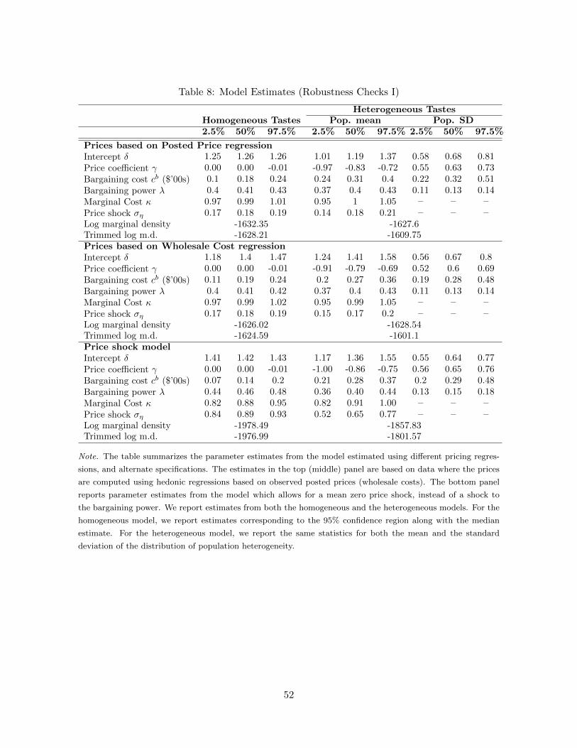
Table 8: Model Estimates (Robustness Checks I)

Heterogeneous TastesHomogeneous Tastes Pop. mean Pop. SD2.5% 50% 97.5% 2.5% 50% 97.5% 2.5% 50% 97.5%

Prices based on Posted Price regressionIntercept δ 1.25 1.26 1.26 1.01 1.19 1.37 0.58 0.68 0.81Price coefficient γ 0.00 0.00 -0.01 -0.97 -0.83 -0.72 0.55 0.63 0.73Bargaining cost cb ($’00s) 0.1 0.18 0.24 0.24 0.31 0.4 0.22 0.32 0.51Bargaining power λ 0.4 0.41 0.43 0.37 0.4 0.43 0.11 0.13 0.14Marginal Cost κ 0.97 0.99 1.01 0.95 1 1.05 – – –Price shock ση 0.17 0.18 0.19 0.14 0.18 0.21 – – –Log marginal density -1632.35 -1627.6Trimmed log m.d. -1628.21 -1609.75Prices based on Wholesale Cost regressionIntercept δ 1.18 1.4 1.47 1.24 1.41 1.58 0.56 0.67 0.8Price coefficient γ 0.00 0.00 -0.01 -0.91 -0.79 -0.69 0.52 0.6 0.69Bargaining cost cb ($’00s) 0.11 0.19 0.24 0.2 0.27 0.36 0.19 0.28 0.48Bargaining power λ 0.4 0.41 0.42 0.37 0.4 0.43 0.11 0.13 0.14Marginal Cost κ 0.97 0.99 1.02 0.95 0.99 1.05 – – –Price shock ση 0.17 0.18 0.19 0.15 0.17 0.2 – – –Log marginal density -1626.02 -1628.54Trimmed log m.d. -1624.59 -1601.1Price shock modelIntercept δ 1.41 1.42 1.43 1.17 1.36 1.55 0.55 0.64 0.77Price coefficient γ 0.00 0.00 -0.01 -1.00 -0.86 -0.75 0.56 0.65 0.76Bargaining cost cb ($’00s) 0.07 0.14 0.2 0.21 0.28 0.37 0.2 0.29 0.48Bargaining power λ 0.44 0.46 0.48 0.36 0.40 0.44 0.13 0.15 0.18Marginal Cost κ 0.82 0.88 0.95 0.82 0.91 1.00 – – –Price shock ση 0.84 0.89 0.93 0.52 0.65 0.77 – – –Log marginal density -1978.49 -1857.83Trimmed log m.d. -1976.99 -1801.57

Note. The table summarizes the parameter estimates from the model estimated using different pricing regres-

sions, and alternate specifications. The estimates in the top (middle) panel are based on data where the prices

are computed using hedonic regressions based on observed posted prices (wholesale costs). The bottom panel

reports parameter estimates from the model which allows for a mean zero price shock, instead of a shock to

the bargaining power. We report estimates from both the homogeneous and the heterogeneous models. For the

homogeneous model, we report estimates corresponding to the 95% confidence region along with the median

estimate. For the heterogeneous model, we report the same statistics for both the mean and the standard

deviation of the distribution of population heterogeneity.

52

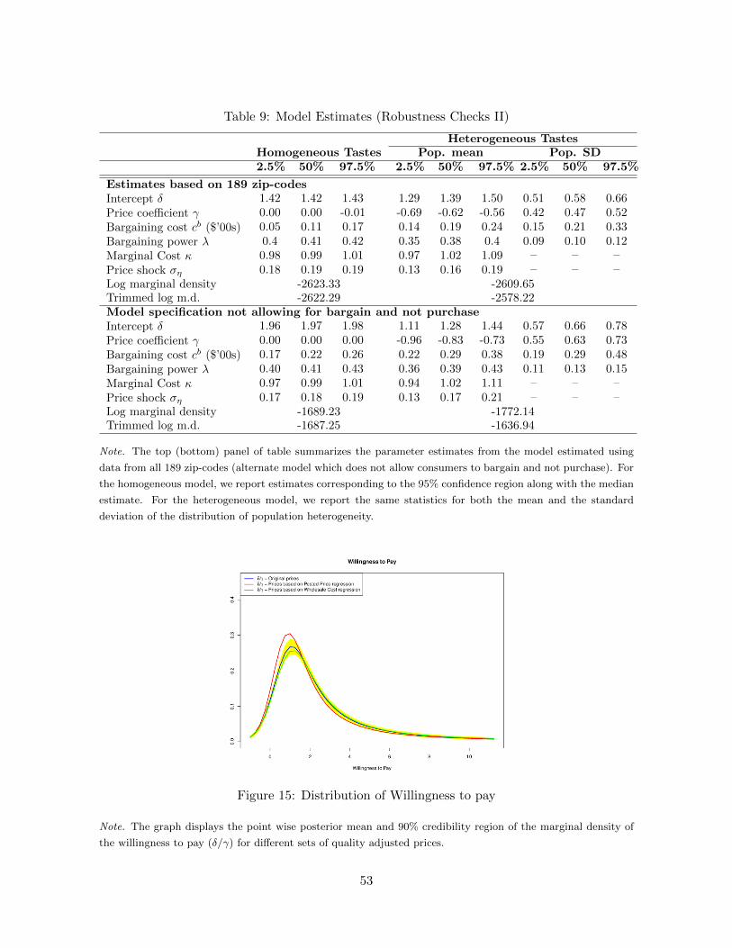
Table 9: Model Estimates (Robustness Checks II)

Heterogeneous TastesHomogeneous Tastes Pop. mean Pop. SD2.5% 50% 97.5% 2.5% 50% 97.5% 2.5% 50% 97.5%

Estimates based on 189 zip-codesIntercept δ 1.42 1.42 1.43 1.29 1.39 1.50 0.51 0.58 0.66Price coefficient γ 0.00 0.00 -0.01 -0.69 -0.62 -0.56 0.42 0.47 0.52Bargaining cost cb ($’00s) 0.05 0.11 0.17 0.14 0.19 0.24 0.15 0.21 0.33Bargaining power λ 0.4 0.41 0.42 0.35 0.38 0.4 0.09 0.10 0.12Marginal Cost κ 0.98 0.99 1.01 0.97 1.02 1.09 – – –Price shock ση 0.18 0.19 0.19 0.13 0.16 0.19 – – –Log marginal density -2623.33 -2609.65Trimmed log m.d. -2622.29 -2578.22Model specification not allowing for bargain and not purchaseIntercept δ 1.96 1.97 1.98 1.11 1.28 1.44 0.57 0.66 0.78Price coefficient γ 0.00 0.00 0.00 -0.96 -0.83 -0.73 0.55 0.63 0.73Bargaining cost cb ($’00s) 0.17 0.22 0.26 0.22 0.29 0.38 0.19 0.29 0.48Bargaining power λ 0.40 0.41 0.43 0.36 0.39 0.43 0.11 0.13 0.15Marginal Cost κ 0.97 0.99 1.01 0.94 1.02 1.11 – – –Price shock ση 0.17 0.18 0.19 0.13 0.17 0.21 – – –Log marginal density -1689.23 -1772.14Trimmed log m.d. -1687.25 -1636.94

Note. The top (bottom) panel of table summarizes the parameter estimates from the model estimated using

data from all 189 zip-codes (alternate model which does not allow consumers to bargain and not purchase). For

the homogeneous model, we report estimates corresponding to the 95% confidence region along with the median

estimate. For the heterogeneous model, we report the same statistics for both the mean and the standard

deviation of the distribution of population heterogeneity.

Figure 15: Distribution of Willingness to pay

Note. The graph displays the point wise posterior mean and 90% credibility region of the marginal density of

the willingness to pay (δ/γ) for different sets of quality adjusted prices.

53

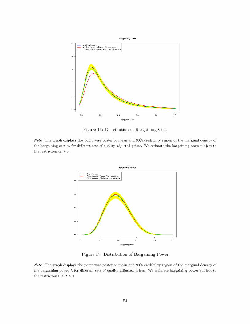
Figure 16: Distribution of Bargaining Cost

Note. The graph displays the point wise posterior mean and 90% credibility region of the marginal density of

the bargaining cost cb for different sets of quality adjusted prices. We estimate the bargaining costs subject to

the restriction cb ≥ 0.

Figure 17: Distribution of Bargaining Power

Note. The graph displays the point wise posterior mean and 90% credibility region of the marginal density of

the bargaining power λ for different sets of quality adjusted prices. We estimate bargaining power subject to

the restriction 0 ≤ λ ≤ 1.

54