Price evolutions on the commodity markets.

Departement Handelswetenschappen en Bestuurskunde

Masterproef

PRICE EVOLUTIONS ON THE COMMODITY MARKETS:

DETERMINANTS IN NORMAL AND CRISIS PERIODS

Tim De Smedt

Master Handelswetenschappen

Afstudeerrichting Finance and Risk Management

Promotor: Dr. Koen Inghelbrecht

Academiejaar 2010-11

2

PRICE EVOLUTIONS ON THE COMMODITY MARKETS:

DETERMINANTS IN NORMAL AND CRISIS PERIODS

MASTER THESIS

Academic Year 2010-2011

Author: Tim De Smedt

Promotor: Koen Inghelbrecht, PhD

4

ABSTRACT

Through a univariate OLS model, we investigate which variables are responsible for price evolutions in commodity spot prices. The variables we investigated were: the future-spot spread (proxy for inventories), oil price (to measure spill-over effects), expected inflation, real interest rate, dollar exchange rate, industrial production, money supply, a crisis dummy and a Black Swan dummy. For all these independent variables (excluding the crisis and black swan dummy), we also added a crisis interaction dummy to measure their effect in times of crisis. Our regression outputs (we performed several) showed us that the future-spot spread, oil, interest rates during a crisis and the exchange rate were responsible for most of the price changes in commodity prices. A multivariate VAR model showed us that changes in commodity prices are Granger Caused by lags of itself and changes in industrial production. We also determined the presence of an industrial production channel through which monetary variables influence the prices of commodities. Impulse responses showed us the impact of exogenous shocks given to the independent variables. In most cases the effect disappears after 1 year.

PRELUDE

This master thesis is written in English, as you, most cautious reader already might have noticed. This is done for two reasons.

Firstly, most of scientific literature these days is written in English. I find it not more than normal, that in our modern society and school system a thesis that is deemed (and urged) to be of a certain scientific level is written in English as well.

Furthermore, a thesis in English might open some doors for me in the future should I opt for a career abroad. The fact that it is already written in English saves me the burden of translating it from Dutch to English should the need arise.

I would like to apologize to the reader for the size of this work. It has become a bit larger than I had originally anticipated, but I wanted to deliver a thesis that was as complete as possible.

Furthermore, the research process kept providing me with more and more exiting results, which I couldn’t exclude. Even now I feel that despite its massive size, there are still many questions unanswered in regard to the studied subject.

To end this prelude I would like to thank my promoter, Koen Inghelbrecht, PhD, for his support, guidance and comments on earlier versions of this master thesis. This thesis wouldn’t have been what it is today without your help.

I hope that you, dear reader, enjoy reading this work as much as I enjoyed writing it.

Kind regards,

Tim De Smedt

Buggenhout, May 22, 2011.

6

CONTENTS

1. Introduction ........................................................................................................... 8

2. Basic concepts .................................................................................................... 10

2.1 Definition ...................................................................................................... 10

2.2 Commodity Markets ..................................................................................... 10

2.2.1 The spot market .................................................................................... 11

2.2.2 The forward market ............................................................................... 11

2.2.3 The futures market ................................................................................ 11

2.3 The term structure of commodity futures ...................................................... 12

2.4 Commodity futures return ............................................................................. 14

2.5 Commodity Indices ....................................................................................... 15

3. Literature overview .............................................................................................. 17

3.1 Price evolutions of commodities and its determinants .................................. 17

3.2 Crisis periods and Black Swans ................................................................... 21

3.3 The financialization of commodity Markets ................................................... 22

4. Research questions and Methodology ................................................................. 25

5. The variables ....................................................................................................... 26

5.1 Commodity Prices ........................................................................................ 26

5.2 Inventories ................................................................................................... 27

5.3 US Money Supply ........................................................................................ 31

5.4 Expected Inflation ......................................................................................... 31

5.5 Real Interest Rates ...................................................................................... 33

5.6 Industrial Production..................................................................................... 34

5.7 Spill-over Effects .......................................................................................... 35

5.8 The Dollar Exchange Rate ........................................................................... 36

5.9 Crisis events ................................................................................................ 37

5.10 Black Swan Events ...................................................................................... 38

5.11 Summary ...................................................................................................... 38

6. The Model ........................................................................................................... 39

6.1 The Basic Model .......................................................................................... 39

6.2 Transformations ........................................................................................... 39

6.2.1 Logaritms .............................................................................................. 39

6.2.2 First Differences (Unit Root Testing) ..................................................... 40

6.2.3 Co-integration relations ......................................................................... 42

6.3 The Final Model ........................................................................................... 43

6.4 Descriptive Statistics .................................................................................... 43

6.4.1 Summary Statistics ............................................................................... 43

7

6.4.2 XY-Plots and Correlation ........................................................................45

7. The univariate model: OLS-regression .................................................................52

7.1 OLS-regressions and tests ............................................................................52

7.2 Prelude: OLS on levels..................................................................................52

7.3 Basic regression: first differences ..................................................................53

7.4 Omitting variables: new regressions ..............................................................57

7.5 A Final OLS regression .................................................................................59

7.6 Aside on lagged variables .............................................................................61

7.7 Choosing the right model ..............................................................................61

8. The multivariate Model: VAR ................................................................................61

8.1 Vector Autoregression ...................................................................................61

8.2 Lag selection .................................................................................................62

8.3 The Model .....................................................................................................62

8.3.1 The Equation ..........................................................................................62

8.3.2 Granger Causality and the Industrial Production Channel .........63

9. Impulse responses ...............................................................................................64

10. Conclusion ........................................................................................................69

11. Overview of Tables, Graphs and figures ...........................................................72

11.1 Graphs ..........................................................................................................72

11.2 Tables ...........................................................................................................73

11.3 Figures ..........................................................................................................73

12. Bibliography ......................................................................................................74

Websites ..................................................................................................................74

Non-Scientific Sources.............................................................................................74

Scientific Sources ....................................................................................................75

Books ...................................................................................................................75

Papers..................................................................................................................75

Scientific Journals ................................................................................................76

8

1. INTRODUCTION Commodities are everywhere. You hear about oil and gold rising to levels never heard of. You see the price of copper rising to such levels that stealing it becomes a very lucrative business. You taste the bitterness of the silver price dropping more than 20 % in one week. Commodities have reached unprecedented highs and scaring depths in the last few years. And they are everywhere…

But what are they exactly? How are they priced? By which factors are they influenced? Now that commodities are available as an alternative source to invest hard earned savings in, we deem it necessary to know which variables are responsible for the price evolutions on the commodity markets. This in order to, at least, shed some light onto the shiny grains of gold, drops of oil or wires of copper we put our money in.

In the literature, as we shall see, there are different paths followed. Researchers focus on the fundamentals (supply and demand) or on the impact monetary policy has on the prices of commodities, sometimes even in regime shifting environments. Or they focus on the impact oil has on other commodities.

The impact of inventories on prices is examined and the role of speculation is looked into. Research involves the study of booms and busts in commodities, over several periods of time, and looks into the role of futures.

All this research, however, often focused just on a single commodity, or a certain subclass. Only rarely a more general approach was taken by looking at a whole basket of commodities (through the use of an index). Also the number of variables researchers put into their models was limited. We also found that the literature involving the impact of crisis periods on commodity prices was rather rare.

These shortcomings we will try to overcome, by using a general model, which incorporates a large(r) amount of variables, whilst also looking into the impact a crisis might have on the prices of commodities. We combine the variables that were used throughout several research paths in the literature into one single model. And while we are at it, we add some interesting new variables as well, like a proxy for inventories and a Black Swan dummy.

Now we know the questions we pose ourselves. We had a glimpse on previous research and on the approach we will take to find some answers. Let us now look at the path we will follow in order to find those answers.

First, we will go over some basic concepts , in order to be able to understand the very nature of the commodities we are investigating. Once some definitions are known, and some insight is gained into the term structure of commodities we move on.

We will give an overview of the scientific literature that we have found. We will look at what authors have written about the price evolutions of commodities and its determinants. We show some things about crisis periods and Black Swans. And we will talk about the financialization of the commodity markets, better known by the dreaded word: Speculation.

Once we dug through all this literature we present you the research questions and the tools we will use to find an answer to these questions.

9

After that, we will introduce the variables . These are the determinants we believe to be responsible for the price evolutions on the commodity markets.

Now that we have knowledge of the scientific literature, stated our research question and introduced the variables it is time to create an econometric model . This is not done in 1-2-3, but requires some transformations in order to make our variables econometrically feasible.

Once that task is complete, we go over some descriptive statistics , in order to get a first glimpse of the impact our select club of variables has on the evolutions of commodity prices.

Then we move on to our univariate model and we perform several OLS regressions in order to find out which determinants are really responsible for price evolutions of commodities.

Once we have a suitable answer on our main question, we move on to our multivariate VAR model . With this model, we will try to determine which variables cause the price evolutions, and we will have a look at the impact exogenous shocks given to the independent variables have on the dependent variable.

This thesis then ends with a conclusion , where we give an overview of our results and try to give some advice to policy makers, investors and future researchers.

10

2. BASIC CONCEPTS

In this chapter we will present some definitions and concepts that are in our opinion necessary for a good understanding of this thesis.

2.1 DEFINITION

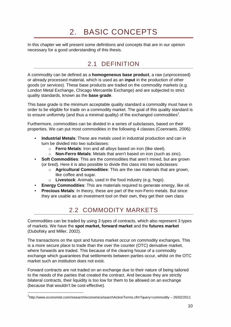
A commodity can be defined as a homogeneous base product , a raw (unprocessed) or already processed material, which is used as an input in the production of other goods (or services). These base products are traded on the commodity markets (e.g. London Metal Exchange, Chicago Mercantile Exchange) and are subjected to strict quality standards, known as the base grade .

This base grade is the minimum acceptable quality standard a commodity must have in order to be eligible for trade on a commodity market. The goal of this quality standard is to ensure uniformity (and thus a minimal quality) of the exchanged commodities1.

Furthermore, commodities can be divided in a series of subclasses, based on their properties. We can put most commodities in the following 4 classes (Coenraets, 2006):

• Industrial Metals : These are metals used in industrial production and can in turn be divided into two subclasses:

o Ferro Metals : Iron and all alloys based on iron (like steel). o Non-Ferro Metals : Metals that aren’t based on iron (such as zinc).

• Soft Commodities : This are the commodities that aren’t mined, but are grown (or bred). Here it is also possible to divide this class into two subclasses:

o Agricultural Commodities : This are the raw materials that are grown, like coffee and sugar.

o Livestock : Animals, used in the food industry (e.g. hogs). • Energy Commodities : This are materials required to generate energy, like oil. • Precious Metals : In theory, these are part of the non-Ferro metals. But since

they are usable as an investment tool on their own, they get their own class

2.2 COMMODITY MARKETS

Commodities can be traded by using 3 types of contracts, which also represent 3 types of markets. We have the spot market, forward market and the futures market (Dubofsky and Miller, 2002).

The transactions on the spot and futures market occur on commodity exchanges. This is a more secure place to trade than the over the counter (OTC) derivative market, where forwards are traded. This because of the clearing house of a commodity exchange which guarantees that settlements between parties occur, whilst on the OTC market such an institution does not exist.

Forward contracts are not traded on an exchange due to their nature of being tailored to the needs of the parties that created the contract. And because they are strictly bilateral contracts, their liquidity is too low for them to be allowed on an exchange (because that wouldn’t be cost-effective).

1http://www.economist.com/research/economics/searchActionTerms.cfm?query=commodity – 26/02/2011

11

2.2.1 THE SPOT MARKET

The spot market is the market where commodities are paid and delivered within 2 days after the sale takes place. Contracts on this market are executed immediately (“on the spot”).The spot market is also referred to as the “cash market”, since transactions are settled in cash at the price that is valid at the moment of the trade. This price is called the spot price2.

Also futures with delivery within a month are traded at the spot price. Trading of these contracts ,however, still occurs on the futures market.

2.2.2 THE FORWARD MARKET

A forward contract is a financial contract that gives the owner the right and obligation to buy a specified commodity on a certain date at a predetermined price. The seller of the forward contract, on the other hand, has the right and obligation to sell the commodity on the predetermined date at the agreed price. At the end of the contract the commodity is delivered and payment will occur. The maturity of a forward contract varies from a period of 3 days to 5 years.

Forward contracts are traded over-the-counter (OTC) , which means they are privately negotiated between the buyer and seller and are often tailored to the specific needs of the parties, like for example to hedge against a specific risk. A consequence of this customization is that these contracts are not easily traded, thus liquidity is very low.

Payments are only done at the time of execution of the contract, but it might be possible that the dealers of forward contracts require collateral. This collateral is an insurance against the possibility that the counterparty will default (Dubofsky and Miller, 2002).

This counterparty risk is inherent to the forward market (which is an OTC derivative market), since there is no such thing as a clearinghouse or frequent trade of forward contracts (liquidity of the market). A possible other solution against this counterparty risk is the creation of a CCP, a central clearing party, that works like a clearinghouse does on a regular exchange3.

2.2.3 THE FUTURES MARKET

A future is a financial contract that gives the owner the right and obligation to buy a commodity on a certain date at a predetermined price. The seller of the future contract has the right and obligation to sell the commodity on the predetermined date at the agreed price. At the end of the contract the commodity is delivered and payment will occur. The maturity of a future contract varies from a period of 3 days to 5 years.

As you can see, a future is similar to a forward contract, except for the following differences. First of all, futures are standardized contracts , which means that they are more liquid than forwards.

2 http://www.economist.com/research/economics/searchActionTerms.cfm?query=spot+market – 27/02/2011 3 The discussion about the necessity of a CCP falls beyond the scope of this thesis. For more information on this subject, see: OTC derivatives and post- trading infra structures, ECB Eurosystem, September 2009

12

Secondly, because of this increased liquidity, futures are traded on exchanges , which in turn lowers the counterparty risk (the clearinghouse of the exchange guarantees payment).

Finally, futures contracts are marked to market , which means that are resettled on a daily basis (Dubofsky and Miller, 2002). These daily changes in the contract price also lowers the risk, because the parties can see how the price evolves. The following table gives a clear overview of the differences between forwards and futures.

Table 1: Differences between forwards and futures Forwards Futures

Private contract between 2 parties Exchange traded Customized contract (tailored) Standard contract

1 specified delivery date Range of delivery dates Settled at maturity Settled daily

Delivery or final cash settlement usually occurs

Contract usually closed out prior to maturity

Source: Fundamentals of futures and options markets, John C. Hull, fourth edition, 2001.

The price of a future will on one hand be determined by the supply and demand for it, and on the other hand by price of the underlying commodity where it is derived from. Eventually though, the price of a future is based on the expectations of the various trading parties. So a future gives an indication of the expected price of a commodity.

In reality, future contracts will seldom be exercised when they come to maturity. This happens, because at the closing of the futures contract it wasn’t the intention of the seller of the contract to actually deliver the goods. Also the buyer of a future never had the intention to actually buy the commodities, but to hedge against the risk of price changes of this specific commodity (or to speculate on them).

The position of the futures contract is offset by taking an opposite position in the same contract type. The buyer of the future sells it back at the seller before the future comes to maturity. Profits or losses are settled in cash at the end of the contract, so there is no exchange of the underlying commodity (De Standaard, 2005).

In some cases a party might want to hold a position in futures for a longer period than the actual maturity of that futures contract (for example 3 month futures). In this case, the owner of the future needs to sell it, just before it reaches its maturity, and then buy a new future (again a 3 month future) which has the same underlying commodity, but a later expiration date. This transaction is called a future roll , because the future is rolled over to a later maturity date.

2.3 THE TERM STRUCTURE OF COMMODITY FUTURES

When we look at the behavior of the prices of commodity futures, as compared to the spot prices of those commodities, there are 2 possible term structures: Backwardation and contango.

When the spot price is higher than the future price with maturity in three months, and this futures price in turn lies higher than the future price with maturity in six months, then we are in a situation which is called backwardation . In this case there is a negative futures curve.

13

This represents the premium a commodity buyer is willing to pay in order to get immediate delivery of a commodity (De Standaard, 2005). On the other side, the seller of a commodity is willing to accept a future price that is lower than the spot price in exchange for the certainty that his commodity will get sold at the predetermined price, i.e. he hedges against changes in the spot price (KBC Securities, November 2010).

When we have backwardation, this means that the current demand for a certain commodity is larger than the demand that is expected in the future. Because of this higher demand in the present, the spot price (the present price) will be higher than the futures price. A market with backwardation gives a signal that traders expect a decline in demand, and thus in prices.

When contango occurs, the spot price will be lower than the futures price. Contango is de facto the opposite of backwardation, and is represented by a positive futures curve. In this case the market expects an excess of supply, or there happens a sudden (unexpected) decline in demand, which causes the spot price to fall. Also, the higher future price incorporates costs for storage, transportation and insurance of the commodities.

When the market is in contango, market parties expect prices to rise in the future (Coenraets, 2006). This is the normal situation on the commodity markets.

The following graph shows the term structure of two commodity futures. On the left hand scale the gold futures are in a state of contango, whilst on the right hand scale the copper futures are in a state of backwardation. The graph clearly shows that these two term structures are opposites of each other.

Graph 1: The term structure of commodity futures

Source: I want to break free or, Strategic Asset Allocation ≠ Static Asset Allocation, GMO, James Montier, May 2010, p.10

14

2.4 COMMODITY FUTURES RETURN

The return of investments in commodity futures has four distinctive components: The spot return, the collateral return, the recomposition yield and the roll yield.

The spot return is the change in the spot price of the underlying commodity between the moment of purchase and the moment the future is sold again.

When agents invest in commodities, they take precautions against possible losses. These precautions come in the form of collateral that these investors set aside as a margin. The collateral return is the return they earn on this collateral (UNCTAD, 2009). This is also referred to as the cash return (KBC Securities, November 2010), since the collateral comes in the form of cash, which is then invested on the money market (and thus generates an extra return this way).

Another part of the return of investing in commodities is the recomposition yield . This yield arises from a periodic redefinition of the basket of commodities that is part of an investment portfolio (UNCTAD, 2009).

The roll yield is the return investors get when the future is rolled over into another future with a later date of maturity. If the term structure knows a negative slope (backwardation), thus when the price of a future that reaches maturity (the one that needs to be sold) is higher than the price of a future with a longer maturity (the future that needs to be bought), than selling the first and buying the latter will result in a profit.

However, when the market has a positive term structure (contango), the roll yield will be negative. The future that needs to be sold will have a lower price than the one with a longer maturity that needs to be bought, which results in a loss (since you have to pay more for the new future than you got from the old one).

The roll yield can be seen as a sort of risk premium that financial investors require for taking a position opposite to that of hedgers (which use futures to limit their price risk). The roll yield is different in one aspect: the contract isn’t held until maturity.

One of the original purposes of futures contracts was to transfer the price risk from market participants that have an interest in the underlying commodity to other participants, willing to take the price risk (UNCTAD, 2009). The commercial market participant (i.e. the participant with an interest in the underlying commodity) pays some sort of (insurance) premium for the transfer of that risk (in the form of the hedging cost) and the counterparty receives this as a premium for assuming the risk.

This risk premium encompasses the difference between the current future price and the expected future spot price, both at the time the future contract is purchased. However, there is no certainty yet at this point which party will benefit from the contract.

When the futures price is lower than the expected future spot price, then the investor (or speculator if you will) will have earned his risk premium. Otherwise, if the price of the future is higher than the expected future spot price, than it will be the seller of the futures contract that earns the premium.

In a normal situation hedgers would outnumber speculators and thus the futures price would be lower than the expected future spot price. This means that speculators wouldn’t earn their risk premium when the contract reaches maturity.

15

If we transfer this to the (slightly different) roll yield, we see the same occurring (the contract just isn’t held till the expiration date).

Research (UNCTAD, 2009) has shown something peculiar. Because of the huge amount of investors in the commodity markets that take long positions in commodities, the term structure has changed from backwardation to contango. This happens because, when a large number of parties takes long positions, there won’t be enough counterparties willing to cover that position.

The prices of futures will be higher when maturity increases, resulting in losses for the financial investors. So, ironically, the enormous interest of financial investors, which have no commercial interest in the underlying commodity, (they already account for almost 50 % of transactions in commodity futures markets) have caused the roll yield, which made investments in commodities in the 80s and 90s so attractive, to become negative (Montier, 2010).

The following graph illustrates this. There was a positive roll yield in the period 1970-2000. But at the last decennium, we can see that the roll yield has become negative, whilst the spot return amounts for most of the return in commodities. The relative importance of the collateral return has diminished, mostly due to low interest rates.

Figure 1: Breakdown of commodity futures returns

Source: I want to break free or, Strategic Asset Allocation ≠ Static Asset Allocation, GMO, James Montier, May 2010, p.11

2.5 COMMODITY INDICES

The best way to measure the prices of commodities is through the use of commodity indices. These indices are made up from a basket of commodities, starting at a certain base year. There are several indices in existence, such as the CRB Index4, the Thomson Reuters Indices5 and the S&P GSCI (and many more).

For the purposes of this thesis we will only focus on the index that is in our opinion the best representation of the role commodities play in the world economy.

4 http://www.crbtrader.com/crbindex/spot_background.asp - 01/03/2011 5http://thomsonreuters.com/products_services/financial/thomson_reuters_indices/indices/commodity_indices/#tab1 – 01/03/2011

16

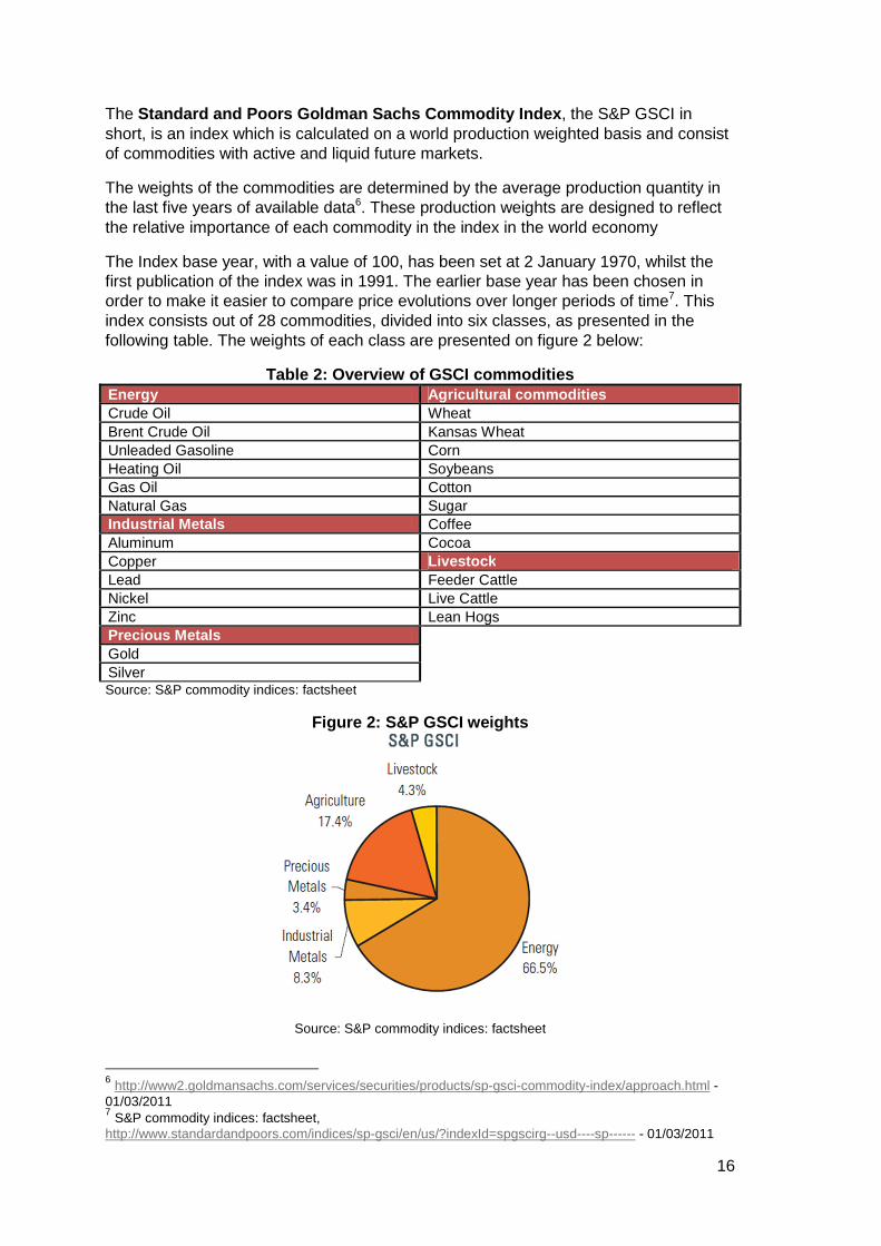
The Standard and Poors Goldman Sachs Commodity Index , the S&P GSCI in short, is an index which is calculated on a world production weighted basis and consist of commodities with active and liquid future markets.

The weights of the commodities are determined by the average production quantity in the last five years of available data6. These production weights are designed to reflect the relative importance of each commodity in the index in the world economy

The Index base year, with a value of 100, has been set at 2 January 1970, whilst the first publication of the index was in 1991. The earlier base year has been chosen in order to make it easier to compare price evolutions over longer periods of time7. This index consists out of 28 commodities, divided into six classes, as presented in the following table. The weights of each class are presented on figure 2 below:

Table 2: Overview of GSCI commodities Energy Agricultural commodities Crude Oil Wheat Brent Crude Oil Kansas Wheat Unleaded Gasoline Corn Heating Oil Soybeans Gas Oil Cotton Natural Gas Sugar Industrial Metals Coffee Aluminum Cocoa Copper Livestock Lead Feeder Cattle Nickel Live Cattle Zinc Lean Hogs Precious Metals Gold Silver Source: S&P commodity indices: factsheet

Figure 2: S&P GSCI weights

Source: S&P commodity indices: factsheet

6 http://www2.goldmansachs.com/services/securities/products/sp-gsci-commodity-index/approach.html - 01/03/2011 7 S&P commodity indices: factsheet, http://www.standardandpoors.com/indices/sp-gsci/en/us/?indexId=spgscirg--usd----sp------ - 01/03/2011

17

3. LITERATURE OVERVIEW In this section we will give an overview of the research that has been done about the determinants of commodity prices and price evolutions in recent scientific literature.

This part will be divided in three chapters. The first chapter will be about the research on price evolutions of commodities and its determinant s. A second chapter will focus on the crisis periods and Black Swan events that might have a profound effect on the prices of commodities. Finally we will look into the role that the financial markets play on the commodity markets in recent years and their impact on prices.

3.1 PRICE EVOLUTIONS OF COMMODITIES AND ITS DETERMINANTS

Early research on the determinants of commodity prices relied solely on demand as the fundamental factor. Demand alone, however, was insufficient to explain weaknesses in commodity prices in the 1980s and 1990s. Borenszstein and Reinhart (1994) extended the model. They added supply and extended demand beyond the demand for commodities in the industrialized world. The view of what was fundamental for commodity prices was widened. However, the focus still lay solely on supply and demand as explanatory variables for the prices of commodities.

Cashin and McDermott (2001) took a different approach and investigated the behavior of commodity prices over a period of almost 140 years (1862-1999) by using the longest dataset available (The Economist’s index of industrial commodity prices). They discovered that there has been a downward trend in commodity prices over this long period of about 1.3% a year. They found no evidence that there would come an end to this trend.

Although this might look like a grim situation, evidence was also found that the variability of commodity prices has been rising. A first hike of variability started in the 1900s and a second increase appeared in the early 1970s, when there came an end to the system of fixed exchange rates. The figure below illustrates this.

Figure 3: Percentage change in real industrial comm odity prices 1862-1999

Source: IMF working paper WP/01/68, The long-run behavior of commodity prices: small trends and big

variability, Paul Cashin and C. John McDermott, May 2001, p. 16

18

This rise in variability, when exchange rates began to float against each other, is already a first indication that exchange rates might have a profound effect on commodity prices, as will be proven later on (IMF, 2008; Akram,2009).

While there is a long running downward trend in commodity prices, this trend is irrelevant since it is quite small and offset entirely by the high variability in prices .

Cashin, McDermott and Scott (2002) expanded the research on commodity price evolutions and investigate the “duration and magnitude of cycles in world commodity prices”. They discovered four characteristics of commodity price booms and slumps :

1. There is an asymmetry in commodity price cycles: Slumps last longer than price booms.

2. Prices appear to fall more in a slump than they rebound in a sub-sequent boom. 3. Cycles of commodity prices don’t appear to have a pattern. The magnitude of

price booms or slumps has nothing to do with the duration. 4. The chance that a slump (boom) ends is independent of the time already spent

in that slump (boom).

It is indeed interesting to know the behavior of commodity prices when in certain situations, but this does not tell us anything about the causes of these booms or slumps. Radetzki (2006) looked into this and studied three separate commodity booms, looking for the reasons why prices rose.

The first boom in 1950-51 was caused by an inventory buildup in response to the Korean war. A second boom in 1973-74 occurred due to a global harvest failure and by the OPEC price politics. A third boom began in 2004 and ran till 20088, and was fueled (to an extent) by the growth of the emerging economies, most notably China and India.

We now know, however, that there was also a serious speculative factor9 present as shown by an increase of the number of financial market participants on the commodity markets (Conceiçao and Marone, 2008; UNCTAD, 2009).

All booms collapsed and subsequently the world economy stumbled into a recession and excessive inventories were sold out. The author believed the third boom to be more durable. Although it also collapsed, the new boom in commodity prices that is underway is apparently still, for a big part, driven by fundamental factors, like demand in the emerging economies, as was previously determined by Borenszstein and Reinhart (1994). Conceiçao and Marone (2008) studied the drivers and the impact of this boom in the 21 st century.

The boom that lasted till halfway 2008 was the largest one in the last 50 years. It lasted longer than usual, affected more commodities and caused larger price increases. And it appeared to be unexpected, since most forecasts underestimated price increases and even when price increase occurred, most predictions stated that a quick and sharp decreases would follow very soon.

The subsequent slump in the second half of 2008 and in 2009 was over rather quickly, negating the first characteristic of price booms as stated by Cashin, McDermott and Scott (2002). The slump did not last longer than the boom.

8 Own addition, since the boom was still underway when the article was published in 2006. 9 More on the role of speculation in chapter 3.3: The financialization of commodity markets.

19

The boom was a mix of fundamentals, speculation and macroeconomic factors. On the fundamentals side we had the strong demand for commodities and supply constraints. Concerning these supply constraints Roache and Erbil (2010) tried to find out how commodity prices and inventories react to a short-run scarcity shock.

They found a long-run relationship between the spot and future p rice, inventories and interest rates . So when a short-run shock occurs, prices will revert back to a stable equilibrium. The pace of this adjustment to the equilibrium appear to depend on the level of the inventories at the time of the shock.

This brings us to the important role inventories play in the price determination of commodities. Research (Gorton and Rouwenhorst, 2005; IMF, 2008, Frankel and Rose, 2009; Carpantier, 2010; Roache and Erbil, 2010) has shown that there is an inverse relationship between the level of inventories and the prices of commodities. The lower the levels of inventories fall, the more the price will rise (i.e. a form of inverse leverage). This is called the inventory effect10.

Speculation also had a role to play in the commodity boom, in the form of market participants that were fully disconnected from fundamentals that normally drive the commodity markets (Conceiçao and Marone, 2008; UNCTAD, 2009).

Although many commodities experienced increasing price levels and the same had underlying factors that caused these price rises, the weight of these drivers appeared to be very different between commodities. For oil and food the price boom was driven mostly by strong demand and supply constraints. For metals on the other hand, speculation seemed to be the most dominant factor (Conceiçao and Marone, 2008).

A commodity boom of this magnitude has advantages for many commodity exporting developing countries, whilst it is not so good for developed countries and developing countries that are importers of commodities. However, China, which is a net importer of commodities, does not seem to be affected much by this because of the strong manufacturing exports that compensate for commodity imports.

Frankel and Rose (2009) wanted to examine the macro-and micro economic factors that drive commodity prices and wrote a paper about the determinants of agricultural and mineral commodity prices. They implement several previously separately used variables (Frankel 2006; Gorton and Rouwenhorst, 2007; Conceiçao and Marone, 2008), and some new ones into one model

This model includes: Global GDP, real interest rates, inventory levels, measures of uncertainty (volatility) and the spot-forward spread (which measures expectations). The model is used on eleven different commodities. Global output and inflation have a positive effect commodity prices although this effect was rather small. It are the microeconomic variables volatility, inventories and spot-forward-spread that have the strongest effect.

There was little support that easy monetary policy and low interest rates were an important source of upward pressure on real commodity prices. This might indicate that there is more to the monetary policy variable than just the interest rates, as stated by Anzuini, Lombardi and Pagano (2010).

10 More on the relation between inventories and the price of commodities can be found in chapter 5.2.

20

These findings about the role of monetary policy and interest rates were curious, since Frankel (2006) already examined the relationship between monetary policy and agricultural and mineral commodities. He found that low interest rates lead to high commodity prices. He examined this for the US and a series of other countries. The evidence appeared to be impressive and the effect of real interest rates on commodities is significant not only for the US, but also for a whole series of (open) economies.

Also Akram (2009) looked into the role of interest rates and investigates the hypothesis that a decline in real interest rates and the US dollar causes commodity prices to rise. The results from his research suggest that “commodity prices increase significantly in response to reductions in real interest rates.” For certain commodities, like oil, there is evidence of overshooting behavior when the real interest rate changes.

Browne and Cronin (2010), stipulate that there should be a long run relationship between commodity prices, consumer prices and money. They tested this hypothesis on US data and found that there is indeed an equilibrium relationship between commodity prices, money and consumer prices . Commodity and consumer prices appeared to be proportional to the money supply in the long run. The authors state that money has to be added to analyses between commodity and consumer prices, an opinion Anzuini, Lombardi and Pagano (2010) follow.

Their research tells us it is important to understand what the impact of the large monetary policy easing is that happened during and after the recent recession. The authors believe that the monetary easing of the last two years will be responsible for a “new surge in commodity prices”.

Previous literature (Frankel, 2006; Akram, 2009) focused on the interest rate as the sole connection between monetary policy and commodity prices. Researchers of the ECB (Anzuini, Lombardi and Pagano, 2010) think, that interest rates do not fully represent the impact of a monetary policy shock. They add the following variables (beside the interest rate which is represented by the federal funds rate): money stock (M2), consumer price index, industrial production index and a commodity price index.

There is empirical evidence that there is a significant impact of monetary policy on commodity prices (Frankel 2006, Akram 2009, Browne and Cronin 2010, Anzuini, Lombardi and Pagano 2010). More specifically: an expansionary monetary policy shock drives up commodity prices.

Anzuini, Lombardi and Pagano (2010) however found that the variance composition shows that the actual impact of monetary policy on commodity price s is rather small but still significant , as opposed to the findings of Frankel and Rose (2009).

Much research done on the impact of the interest rates and monetary policy focused on the US dollar. Akram (2009) looked, besides the interest rate, at the dollar exchange rate and investigated whether the depreciation of the US dollar leads to higher commodity prices. He discovered that a shock in the dollar exchange rate leads to a significant movement of commodity prices, and indeed a decline of the US dollar exchange rate causes commodity prices to rise.

Akram (2009) states that the value of the dollar (together with the US real interest rate) could be good indicators for the movement of commodity prices. Other research (IMF, 2008; UNCTAD, 2009; Bhar and Hammoudeh, 2010) on the relation of the dollar exchange rate with commodity prices seems to verify this.

21

In the IMF world economic outlook of April 2008, the author examines the relation between the dollar exchange rate and commodity prices. Over the past 20 years commodity prices have been (mostly) negatively corr elated with the US dollar .

The dollar exchange rate has a significant impact on gold and oil prices in the short and long run. A one percent depreciation of the dollar results, in the long run, in a increase of the gold and oil prices with more than one percent. For other commodities there is also an increase, but smaller than one percent.

This difference between commodities can be explained by the fact that commodities such as gold and oil are more usable as a “storage of value”, where this is not really possible with perishable commodities (the impact of the dollar exchange rate on grain, for example is not significant).

The relation between the dollar exchange rate and the oil price has also been found by Bhar and Hammoudeh (2010). They looked at the influence of both interest rates and exchange rates on commodity prices in a regime shifting environment.

The relationship between the dollar and the oil price is negative, which means that in times of crisis, a weakening dollar leads to higher oil prices. In a normal economic state this effect is weaker. This discrepancy between a normal state and a crisis state leads us to the next chapter on crises and Black Swan events.

3.2 CRISIS PERIODS AND BLACK SWANS

Bhar and Hammoudeh (2010) looked, as previously stated, into the influence of several variables on commodity prices in regime shifting environments. Although we won’t go into regime changing environments in this thesis, it is interesting to see what the influence of the various variables is on commodity prices in a normal and crisis period.

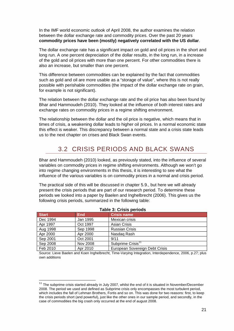
The practical side of this will be discussed in chapter 5.9., but here we will already present the crisis periods that are part of our research period. To determine these periods we looked into a paper by Baelen and Inghelbrecht (2006). This gives us the following crisis periods, summarized in the following table:

Table 3: Crisis periods Start End Crisis name Dec 1994 Jan 1995 Mexican crisis Apr 1997 Oct 1997 Asian Crisis Aug 1998 Sep 1998 Russian Crisis Apr 2000 Apr 2000 Nasdaq Rash Sep 2001 Oct 2001 9/11 Sep 2008 Nov 2008 Subprime Crisis11 Feb 2010 Apr 2010 European Sovereign Debt Crisis Source: Lieve Baelen and Koen Inghelbrecht, Time-Varying Integration, Interdependence, 2006, p.27; plus own additions

11 The subprime crisis started already in July 2007, whilst the end of it is situated in November/December 2008. The period we used and defined as Subprime crisis only encompasses the most turbulent period, which includes the fall of Lehman Brothers, Fortis and so on. This was done for two reasons: first, to keep the crisis periods short (and powerful), just like the other ones in our sample period, and secondly, in the case of commodities the big crash only occurred at the end of august 2008.

22

Besides (relatively frequent) crisis moments, there are also those very rare events, with a huge impact, known as Black Swan events . A Black Swan, a term invented by Nassim Nicholas Taleb (2010), is an event with the following three attributes:

• First of all, a Black Swan event is an outlier , which means that is an event we can’t really expect to occur, based on regular expectations. Nothing in the past points to this event.

• Secondly, a Black Swan event has an enormous impact . • And finally, humans begin to search for logical explanations after the event

took place , in an attempt to make it explainable and predictable.

The interesting thing about these Black Swans is their low predictability and large impact. The rarity of the events, makes people act as if Black Swans don’t exist. Thus believing they could measure uncertainty. So, most measures in modern economic models exclude the possibility of Black Swan events, which implicates that they have “ no better predictive value for assessing the total risk than astrology” (Taleb, 2010).

However, people need some form of model to base expectations upon , even if it is not the right one, or the one that incorporates all possible events (which is, in our opinion, impossible). Thus, the very essence of human nature, the need for those models/reference cadre, makes it hard for us to predict Black Swan events (which lie, per definition, outside those models). It is, however, interesting to see what the impact of such an event might be on commodity prices (even in hindsight).

Therefore we will implement three Black Swan events into our research period. Events that incorporate the three attributes previously mentioned. These events are: The 9/11 terrorist attack on the twin towers (September 2001), the Tsunami of 2004 (December 2004) and finally the fall of Lehman Brothers in September 2008 , triggering a world-wide financial storm and the Great Recession.

3.3 THE FINANCIALIZATION OF COMMODITY MARKETS

We can define the financialization of the commodity markets as the growing presence of financial institutions and players on t he commodity markets who, on the contrary to commercial market participants (like producers of commodities hedging their positions), have no real connection to the underlying commodity. The financial players are driven by motives of portfolio diversification (UNCTAD, 2009). Speculation can be defined as the purchase of a commodity (contract) in anticipation of financial gain at the time of resale (Frankel and Rose, 2009).

It has been said that the recent commodity boom was largely driven by financial players that speculated on commodities. Evidence that prices of commodities are not aligned with fundamentals is not all that clear. Conceiçao and Marone (2008) state that the most conclusive evidence about speculation can be found at the metal commodities, more specifically copper and nickel.

The question that we need to ask ourselves in regard to the boom of 2008 is: How detached were price levels from fundamentals, as co mpared to earlier booms?

23

As you can see in table 4 , for copper, during a trough in the economic cycle in 1985, the ratio of the market price to the marginal production cost (of the least efficient producers) was 1. Meaning that market prices were just sufficient to cover the costs of production. In the case of nickel and aluminum market prices were even too low to cover the marginal production costs of the least efficient producers.

Table 4:Cash Cost of Production of Basic Metals (US dollars per ton)

Source: UNDP working paper, Characterizing the 21st century first commodity boom: Drivers and impact, Pedro Conceiçao and Heloisa Marone, October 2008, p.24

During the last boom, we can see that, compared to marginal costs of 2005, the ratio of price to marginal cost was 2,8 for copper, showing that prices were getting detached from fundamentals, represented here as the marginal costs (the ratio was also much higher than during previous booms). For efficient producers the ratio was even much higher.

Frankel and Rose (2009), have a broader viewpoint and look at speculation from two distinct angles. Firstly speculation can be seen as an major (some might say evil) force that pushed up prices during the commodity boom of 2003-2008, in the absence of fundamental reasons. Thus, a bubble scenario.

A second interpretation on the role of speculation can be a less malevolent one, where speculation (or the activities of financial market participants), can be seen as a stabilizing factor .

In many cases, speculators are often “net short” on commodities, meaning that on average, during a certain period of time, they sold more contracts than they bought. They did this because they anticipated a reversion of prices to normal levels. By going short, based on this expectation, speculators might have kept prices lower than they otherwise would have been.

If we recapitulate this: because the speculators anticipated a possible reversion of commodity prices to normal levels, they took positions on this presumption. And by doing so they kept prices lower or might have even reversed the price rising trend eventually. Almost like a self-fulfilling prophecy.

24

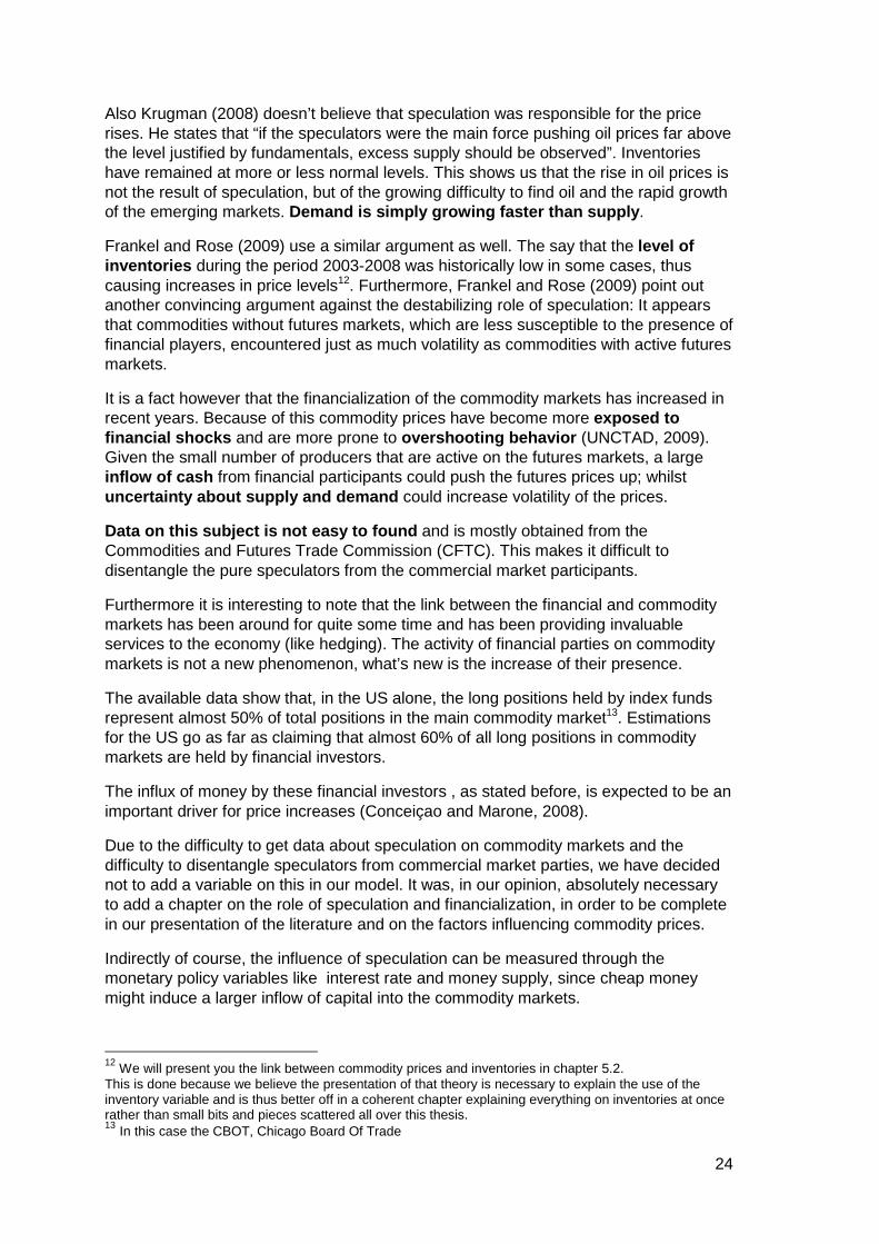
Also Krugman (2008) doesn’t believe that speculation was responsible for the price rises. He states that “if the speculators were the main force pushing oil prices far above the level justified by fundamentals, excess supply should be observed”. Inventories have remained at more or less normal levels. This shows us that the rise in oil prices is not the result of speculation, but of the growing difficulty to find oil and the rapid growth of the emerging markets. Demand is simply growing faster than supply .

Frankel and Rose (2009) use a similar argument as well. The say that the level of inventories during the period 2003-2008 was historically low in some cases, thus causing increases in price levels12. Furthermore, Frankel and Rose (2009) point out another convincing argument against the destabilizing role of speculation: It appears that commodities without futures markets, which are less susceptible to the presence of financial players, encountered just as much volatility as commodities with active futures markets.

It is a fact however that the financialization of the commodity markets has increased in recent years. Because of this commodity prices have become more exposed to financial shocks and are more prone to overshooting behavior (UNCTAD, 2009). Given the small number of producers that are active on the futures markets, a large inflow of cash from financial participants could push the futures prices up; whilst uncertainty about supply and demand could increase volatility of the prices.

Data on this subject is not easy to found and is mostly obtained from the Commodities and Futures Trade Commission (CFTC). This makes it difficult to disentangle the pure speculators from the commercial market participants.

Furthermore it is interesting to note that the link between the financial and commodity markets has been around for quite some time and has been providing invaluable services to the economy (like hedging). The activity of financial parties on commodity markets is not a new phenomenon, what’s new is the increase of their presence.

The available data show that, in the US alone, the long positions held by index funds represent almost 50% of total positions in the main commodity market13. Estimations for the US go as far as claiming that almost 60% of all long positions in commodity markets are held by financial investors.

The influx of money by these financial investors , as stated before, is expected to be an important driver for price increases (Conceiçao and Marone, 2008).

Due to the difficulty to get data about speculation on commodity markets and the difficulty to disentangle speculators from commercial market parties, we have decided not to add a variable on this in our model. It was, in our opinion, absolutely necessary to add a chapter on the role of speculation and financialization, in order to be complete in our presentation of the literature and on the factors influencing commodity prices.

Indirectly of course, the influence of speculation can be measured through the monetary policy variables like interest rate and money supply, since cheap money might induce a larger inflow of capital into the commodity markets.

12 We will present you the link between commodity prices and inventories in chapter 5.2. This is done because we believe the presentation of that theory is necessary to explain the use of the inventory variable and is thus better off in a coherent chapter explaining everything on inventories at once rather than small bits and pieces scattered all over this thesis. 13 In this case the CBOT, Chicago Board Of Trade

25

4. RESEARCH QUESTIONS AND METHODOLOGY

To what extent do several determinants 14 have an impact on the price evolutions of commodities?

That is the question we ask ourselves when looking at the literature and our chosen variables. In order to find an answer to it, we will use a univariate model so we can estimate the impact of the independent variables on commodity prices. This univariate model will consist of an OLS regression of time series data for a sample period ranging from 31/01/1995 till 31/12/2010.

Once we have estimated the model and after we have interpreted the results, we can move on to a second phase. Our OLS-regression will tell us by which variable(s) the commodity spot price is influenced.

This model is, however, subject to the endogeneity problem, which means that the “independent” variables might also be affected by changes of the commodity prices, or by the other independent variables (and not just by exogenous factors). This means that our independent variables might not be so independent as we might believe.

To overcome this problem we will use a multivariate model, namely a VAR (Vector Auto Regression) model . This model will enable us to answer the following question:

Can we determine which variables cause changes in t he commodity prices and vice versa, which changes are caused by a change in commodity prices?

We will examine the impact of the variables on each other for our entire sample period. When we include lagged variables in this model, we might also be able to determine which variables Granger Cause others.

Once we have successfully estimated this VAR model, we will use impulse responses (i.e. we will give exogenous shocks to the variables in the model) to see which impact the change of one variable has on the price of commodities (we will limit ourselves to the impact on the commodity spot prices). This way we might answer the question below:

In which way do the variables in this model have an impact on commodity prices and to what extent?

This might give us some insight in how commodity prices behave and might even give us some possibility to forecast future price movements.

Before we can answer these questions, let us first have a look at the variables and the model we will use in the next few chapters.

14 These determinants, or variables, will be presented in the following chapter.

26

5. THE VARIABLES

5.1 COMMODITY PRICES

The commodity prices will be the dependent variable in this research. As a proxy for the prices of commodities we will use the GSCI spot price index. We opt for this index for three reasons:

(1) It exists since 1991, and consists of actively traded and liquid commodities. (2) The commodities in this index are weighted in such a way that this reflects the

relative importance of each commodity in the world economy15. (3) Since 1995 this index has also a futures version which will enable us to

calculate the Future-spot spread, which is required for one of the variables.

The following graph presents the evolution of the spot Index for the main period to give a first glimpse of the evolution of commodity prices.

As you can see there has been a steady rise in overall commodity prices since 2002. With an extreme growth in 2007, after which they suddenly plunged into the abyss halfway 2008. The decline only halted in 2009, after which a sharp rise once more began, although the high levels of 2008 are not yet reached.

Graph 2: S&P GSCI Commodity Spot - Price Index

Source: Datastream

This dependent variable will be represented in the model as ��.

15 http://www2.goldmansachs.com/services/securities/products/sp-gsci-commodity-index/approach.html - 01/03/2011

100

200

300

400

500

600

700

800

900

1996 1998 2000 2002 2004 2006 2008 2010

Spot_

Price_In

de

27

5.2 INVENTORIES

Inventory levels of various commodities are of importance for the price determination. There should be an inverse relation between inventories and the price of commodities. If inventories are low, prices will be high and vice versa (IMF, 2008). This is presented in the following graph.

Graph 3: Inverse relationship inventories and price s

Source: IMF, World economic outlook, April 2008. p. 57

In order to gather data on this variable, there are some issues. First, there is no common data source where data on commodity inventories worldwide are to be found. The data is scattered around and thus very difficult to gather.

A second problem that poses itself is the definition of an inventory. Are the inventories held (and reported) at the commodity exchanges sufficient? What about (unavailable) data about inventories held off exchange? Or proven reserves that are still in the ground? It is clear that just using data of inventories held at the exchanges is just the tip of the inventory iceberg (UNCTAD, 2009; Carpantier, 2010).

There is also a timing factor issue besides the previously mentioned problems. Data on inventories, if available, is published with a time lag and is often revised several times, lowering the reliability of the data even more (Gorton and Rouwenhorst, 2005).

Only if our research would have been limited to the price evolutions of specific commodities, like for example copper, then the data on the inventories from the London Metal Exchange (LME) could have been a good proxy for copper inventories in general , since about 95 % of the world trade in copper futures happens on the LME (Roache and Erbil, 2010).

In our case, however, this would not work because we look at a broader range of commodities. The use of inventory data to represent the influence of this variable on commodity prices in general, would be too unreliable and incomplete.

So, we had to look for a viable alternative, to represent the inventory variable. This alternative presented itself in the form of the Future-Spot spread , which we will explain in the following paragraphs. In order to understand the use of the future-spot spread as a proxy for the commodity inventories, we have to present you with the theory of storage .

28

This theory implies, that there is a cost adjusted equivalence between buying a future contract (i.e. receive the commodity at a predetermined date at a certain price.) or directly buying and storing a commodity (Carpantier, 2010). These storage costs, which include costs like insurance, interests, transport and the actual storage cost, are called the cost of carry (UNCTAD, 2009) .

This can be represented by the following formula (Carpantier, 2010):

��,�− �� = �� > 0

With: ��,�: Future price, with delivery at time T. ��: Spot price at time t ��: Global cost of storage between time t and T (cost of carry)

In this case, as represented by the formula, the futures prices are higher than the spot price, thus the market is in contango. Although, as previously mentioned, markets aren’t always in this situation, since futures prices can also be lower than spot prices. In this case the market will be in backwardation. Now, the two possible term structures of the commodity markets brings us to the concept of the convenience yield.

The convenience yield , can be defined as the value of having a sufficient amount of a certain commodity in stock in the event of a disruption (Frankel and Rose, 2009). Or otherwise stated: Having a commodity in storage gives a good opportunity to the agent having that commodity in storage.

For example, when there is a sudden oil market disruption, this will lead to a price rise of oil, thus leading to extra yield for agents with oil at their disposal at that moment (when they sell it). This possible benefit for having a commodity in storage is the convenience yield and can be presented by the following formula (Carpantier, 2010):

�� = �� − ��,�+��

With: ��: The convenience yield at time t ��,�: Future price, with delivery at time T.

��: Spot price at time t ��: Global cost of storage between time t and T.

The convenience yield will rise when markets are tight and inventories are low. This represents the positive yield for agents that have the commodity already in stock, ready for direct delivery. Spot prices are higher than futures prices in such a situation, which makes it interesting to sell commodities on the spot.

If we look at the two possible term structures of commodity futures, we get the following two situations:

• Contango: �� − ��,� < � , which results in a negative convenience yield. (�� < 0).Now, when we reverse the calculation, we get ��,� – �� > 0. This situation implies high inventory levels. So it is not that interesting to have commodities in stock, since there is a higher cost of storage due to the high demand for this storage.

• Backwardation: �� − ��,� > � , which results in a positive convenience yield (�� > 0). When we reverse the calculation to get the future spot spread, we get: ��,� - �� < 0. In this case there are low inventory levels, so it is interesting for agents to have a stock of commodities, since prices will rise in the future. Also, due to low demand for storage, the cost of carry will be lower.

29

It has been shown empirically (Gorton, Hayashi and Rouwenhorst, 2008; Roache and Erbil, 2010) that the convenience yield is a decreasing, non-linear function of inventories, as illustrated by the following graph.

Graph 4: Non-linearity of convenience yield and inv entories

Source: IMF working paper, How commodity price curves and inventories react to a short-run scarcity

shock, Shaun Roache and Nese Erbil, September 2010, p.5

This non-linearity implies that, the lower inventory levels get, the higher the convenience yield will be. And a higher convenience yield is linked to a higher spot price. Furthermore, when inventories reach a low level, a further decrease of the inventory levels will have a much larger impact on the price of commodities than an increase in these inventories.

The closer inventories get to a potential stock-out, the larger the impact of the non-linearity will be, or otherwise said: When inventory levels continue to drop, the increase in prices will become larger. This inverse leverage effect, where positive returns result into larger increases of volatility, is called the inventory effect (Carpantier, 2010).

This connection between the price of commodities and the inventory effect, via the convenience yield and the term structure of commodities, implies that the future-spot spread (�� ,� – �� ) can be considered as a valid proxy for commodity inventories: A small spread would imply low inventories and thus a high convenience yield, while a large spread would mean that inventory levels are high and the convenience yield is low.

There should also be a negative correlation between the spot price level and inventories (IMF, 2008). This implies that at high price levels, the spread will have dropped (i.e. it became more negative), thus representing low inventory levels. When commodity inventories rise, the future spot spread rises as well and becomes less negative.

So, a drop in inventories (when demand is bigger than supply) will result in positive price change, meaning the inventory and price curves move in opposite directions, as shown in the following graph.

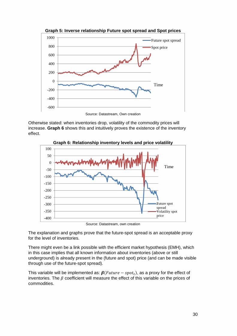
If you look closely to graph 5 on the following page, you will notice that when the future-spot spread drops, the price rises more than the drop of the spread.

30

Graph 5: Inverse relationship Future spot spread an d Spot prices

Source: Datastream, Own creation

Otherwise stated: when inventories drop, volatility of the commodity prices will increase. Graph 6 shows this and intuitively proves the existence of the inventory effect.

Graph 6: Relationship inventory levels and price vo latility

Source: Datastream, own creation

The explanation and graphs prove that the future-spot spread is an acceptable proxy for the level of inventories.

There might even be a link possible with the efficient market hypothesis (EMH), which in this case implies that all known information about inventories (above or still underground) is already present in the (future and spot) price (and can be made visible through use of the future-spot spread).

This variable will be implemented as: �� − !"��, as a proxy for the effect of inventories. The # coefficient will measure the effect of this variable on the prices of commodities.

-600

-400

-200

0

200

400

600

800

1000Future spot spread

Spot price

Time

-400

-350

-300

-250

-200

-150

-100

-50

0

50

100

Future spotspreadVolatility spotprice

Time

31

5.3 US MONEY SUPPLY

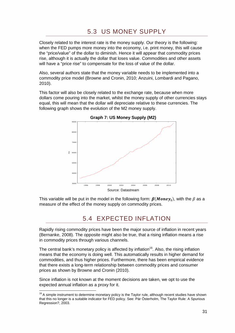
Closely related to the interest rate is the money supply. Our theory is the following: when the FED pumps more money into the economy, i.e. print money, this will cause the “price/value” of the dollar to diminish. Hence it will appear that commodity prices rise, although it is actually the dollar that loses value. Commodities and other assets will have a “price rise” to compensate for the loss of value of the dollar.

Also, several authors state that the money variable needs to be implemented into a commodity price model (Browne and Cronin, 2010; Anzuini, Lombardi and Pagano, 2010).

This factor will also be closely related to the exchange rate, because when more dollars come pouring into the market, whilst the money supply of other currencies stays equal, this will mean that the dollar will depreciate relative to these currencies. The following graph shows the evolution of the M2 money supply.

Graph 7: US Money Supply (M2)

Source: Datastream

This variable will be put in the model in the following form: ��$�%&'��, with the # as a measure of the effect of the money supply on commodity prices.

5.4 EXPECTED INFLATION

Rapidly rising commodity prices have been the major source of inflation in recent years (Bernanke, 2008). The opposite might also be true, that a rising inflation means a rise in commodity prices through various channels.

The central bank’s monetary policy is affected by inflation16. Also, the rising inflation means that the economy is doing well. This automatically results in higher demand for commodities, and thus higher prices. Furthermore, there has been empirical evidence that there exists a long-term relationship between commodity prices and consumer prices as shown by Browne and Cronin (2010).

Since inflation is not known at the moment decisions are taken, we opt to use the expected annual inflation as a proxy for it. 16 A simple instrument to determine monetary policy is the Taylor rule, although recent studies have shown that this no longer is a suitable indicator for FED policy. See: Pär Österholm, The Taylor Rule: A Spurious Regression?, 2003.

3000

4000

5000

6000

7000

8000

9000

1996 1998 2000 2002 2004 2006 2008 2010

M2

32

The data necessary to calculate this variable will be obtained from the “survey of professional forecasters17”. For this variable we used the series CPIB, which represents the forecast for the inflation of the coming year.

This survey, however is taken every quarter, so there are no monthly data, which we need, available. To solve this issue we have transformed the quarterly data into monthly data by taking the forecast of the first quarter (which is taken in the first half of February) and then use this forecast value for the months February, March and April. The forecast for the second quarter is then used for the months May, June and July, and so on, as you can see in the following table.

Table 5: Timing of the Survey of Professional Forec asters

Source: SPF documentation, http://www.philadelphiafed.org/research-and-data/real-time-center/survey-of-

professional-forecasters/spf-documentation.pdf - 30/03/2011

In table 6, we present an example of the data transformation. Because the survey is taken in the first weeks of February, there is always a shift of one month. So in January we use the expected inflation from the November forecast of the previous year.

Table 6: Transformation to monthly data Month quarter Expected

Annual Inflation

Survey from:

31/01/1995 1 3,443 November 1994 28/02/1995 3,596 February 1995 31/03/1995 3,596 February 1995 28/04/1995 2 3,596 February 1995 31/05/1995 3,590 May 1995 30/06/1995 3,590 May 1995 31/07/1995 3 3,590 May 1995 31/08/1995 3,314 August 1995 29/09/1995 3,314 August 1995 31/10/1995 4 3,314 August 1995 30/11/1995 2,878 November 1995 29/12/1995 2,878 November 1995

Source: Survey of professional forecasters, own creation

17 http://www.philadelphiafed.org/research-and-data/real-time-center/survey-of-professional-forecasters/ - 02/03/2011, the file with the data can be found on http://www.philadelphiafed.org/research-and-data/real-time-center/survey-of-professional-forecasters/historical-data/mean-forecasts.cfm , Mean forecast data for levels.

33

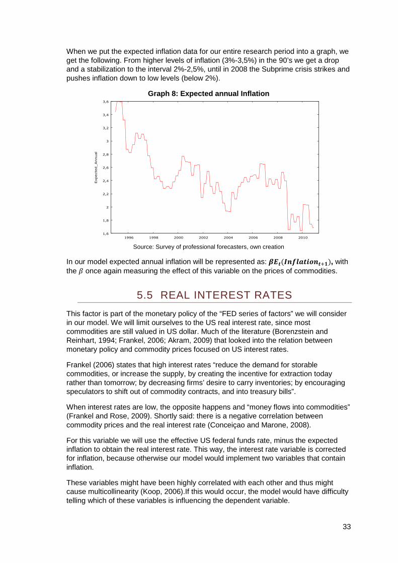
When we put the expected inflation data for our entire research period into a graph, we get the following. From higher levels of inflation (3%-3,5%) in the 90’s we get a drop and a stabilization to the interval 2%-2,5%, until in 2008 the Subprime crisis strikes and pushes inflation down to low levels (below 2%).

Graph 8: Expected annual Inflation

Source: Survey of professional forecasters, own creation

In our model expected annual inflation will be represented as: �(��)%*+,�-�%�./�, with the # once again measuring the effect of this variable on the prices of commodities.

5.5 REAL INTEREST RATES

This factor is part of the monetary policy of the “FED series of factors” we will consider in our model. We will limit ourselves to the US real interest rate, since most commodities are still valued in US dollar. Much of the literature (Borenzstein and Reinhart, 1994; Frankel, 2006; Akram, 2009) that looked into the relation between monetary policy and commodity prices focused on US interest rates.

Frankel (2006) states that high interest rates “reduce the demand for storable commodities, or increase the supply, by creating the incentive for extraction today rather than tomorrow; by decreasing firms’ desire to carry inventories; by encouraging speculators to shift out of commodity contracts, and into treasury bills”.

When interest rates are low, the opposite happens and “money flows into commodities” (Frankel and Rose, 2009). Shortly said: there is a negative correlation between commodity prices and the real interest rate (Conceiçao and Marone, 2008).

For this variable we will use the effective US federal funds rate, minus the expected inflation to obtain the real interest rate. This way, the interest rate variable is corrected for inflation, because otherwise our model would implement two variables that contain inflation.

These variables might have been highly correlated with each other and thus might cause multicollinearity (Koop, 2006).If this would occur, the model would have difficulty telling which of these variables is influencing the dependent variable.

1,6

1,8

2

2,2

2,4

2,6

2,8

3

3,2

3,4

3,6

1996 1998 2000 2002 2004 2006 2008 2010

Expecte

d_Annual

34

If we want to assess the real impact of monetary policy, we have to look at more factors of monetary policy than just the interest rate. This because interest rates alone may not fully capture the impact of monetary policy (shocks) and their movement can be just an endogenous response of monetary policy to general developments in the economy (Anzuini, Lombardi and Pagano, 2010).

This means that the movement of interest rates might just be caused by other variables in the model, like expected inflation or output and not by exogenous factors18.

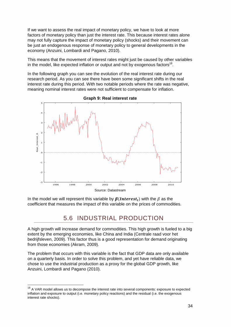
In the following graph you can see the evolution of the real interest rate during our research period. As you can see there have been some significant shifts in the real interest rate during this period. With two notable periods where the rate was negative, meaning nominal interest rates were not sufficient to compensate for inflation.

Graph 9: Real interest rate

Source: Datastream

In the model we will represent this variable by ��)%�&0&1�� with the # as the coefficient that measures the impact of this variable on the prices of commodities.

5.6 INDUSTRIAL PRODUCTION

A high growth will increase demand for commodities. This high growth is fueled to a big extent by the emerging economies, like China and India (Centrale raad voor het bedrijfsleven, 2009). This factor thus is a good representation for demand originating from those economies (Akram, 2009).

The problem that occurs with this variable is the fact that GDP data are only available on a quarterly basis. In order to solve this problem, and yet have reliable data, we chose to use the industrial production as a proxy for the global GDP growth, like Anzuini, Lombardi and Pagano (2010).

18 A VAR model allows us to decompose the interest rate into several components: exposure to expected inflation and exposure to output (i.e. monetary policy reactions) and the residual (i.e. the exogenous interest rate shocks).

-3

-2

-1

0

1

2

3

4

5

1996 1998 2000 2002 2004 2006 2008 2010

Real_

Interest_R

35

The literature (Borenzstein and Reinhart, 1994; IMF, 2008) states that increases in industrial production require more commodity inputs, so industrial production is actually closer related to commodities than GDP.

Since this data is not available for the entire world, we will use an index that represents industrial productivity growth in the OECD-countries (34 members) plus the 6 greatest economies19 that are not a member of this organization20.The following graph gives the evolution of the industrial production for the research period.

Graph 10: Industrial Production

Source: Datastream

On this graph we can see that industrial production has remained quite stable through-out our sample period, with some hikes in 2000-2001 and of course one big rise and subsequent fall in the period 2006 till 2009. We can see that since halfway 2009 industrial production has started to increase again and is already back at the pre-crisis level.

In our model we will represent industrial production as ��)%231�0-,+��, with again the # measuring the impact of this explanatory variable on our dependant variable, the spot price.

5.7 SPILL-OVER EFFECTS

This means that the price change in one commodity passes on to another commodity, whose production process is dependent on the previous commodity (in a direct or indirect way). Through a “cost-push –effect” the more expensive first commodity will cause the second commodity to rise in price as well (Akram, 2009). The price rise of the first commodity pushes the production costs of the second commodity to a higher level.

Crude oil prices affect the prices of other commodities in several ways. Crude oil enters the supply chain when it is used for the production of commodities that require high energy inputs (fuel for agricultural commodity production) or that are very energy intensive in their various processing stages (like aluminum). Also, transportation of commodities requires large quantities of oil. 19 Brazil, China, Russia, India, Indonesia and South-Africa 20 http://www.oecd.org/document/25/0,3746,en_36734052_36761800_36999961_1_1_1_1,00.html – 02/03/2011

92

94

96

98

100

102

104

106

1996 1998 2000 2002 2004 2006 2008 2010

Industria

l_Prod

36

Commodities that can act as a substitute for oil (like gas or coal) will rise in price as well, since demand for them rises as oil becomes more expensive.

High crude oil prices21 increase the available income in oil exporting countries. Because of this, the demand for popular commodities in those countries (like tea and gold) grows. Also, an increase of the oil price is often associated with inflation, which in turn also makes the demand for precious metals, a traditional hedge against inflation, to rise (Baffes, 2007).

To implement this effect into our model, we will use the oil price, here the S&P GSCI Crude Oil Spot price index, as a proxy for this effect, since oil is one of the major spill-over commodities. This graph illustrates the evolution of the oil price, which follows a path similar to the commodity index.

Graph 11: S&P GSCI Crude Oil Spot price index

Source: Datastream

The spill-over effect will be added to our model in the following form: ��4-+��, again with the # measuring the impact of the spill-over effect on commodity prices.

5.8 THE DOLLAR EXCHANGE RATE

The past 20 years there has been a negative correlation between the dollar exchange rate and the price of commodities (IMF, 2008). The exchange rate evolution of the dollar will assert its impact on commodity prices through a number of channels, like purchasing power, investment returns and linked currencies (De Smedt, 2010).

Since it would make the model extremely complex if we add several currencies, we will use an trade weighted average index of the foreign exchange value of the US dollar against the currencies of the major trading partners of the US (Bhar and Hammoudeh, 2010).

An increase in this index will represent an appreciation of the dollar (and a depreciation of the average of the foreign currencies), whilst a decrease will mean a depreciation of the greenback22.

21 For more information about the impact of oil (shocks) on the (macro)-economy, see: Barsky and Kilian and (2004), Rogoff (2006) and Kilian (2007). These are not implemented in the literature overview since their research does not involve the impact of variables (oil in this case) on commodity prices. 22http://www.federalreserve.gov/releases/h10/Summary/ -12/12/2010

0

100

200

300

400

500

600

700

800

1996 1998 2000 2002 2004 2006 2008 2010

Crude_O

il_Spot

37

In the following graph you can see the evolution of this index. We can see here that, compared to the years 2001-2003, the dollar is at a low level and has known a steady decline during the period ranging from 2004 till 2008.

It appears that the crisis triggered a sudden rise in the dollar exchange rate after reaching a very low point in 2008. Although the dollar knew a steep appreciation, this was short-lived because it has now reached pre-crisis levels again.

Graph 12: The dollar exchange rate index

Source: Datastream

This also gives an indication of the negative correlation between the commodity prices and the dollar exchange rate. We can see, that at the moment when commodity prices took a nose dive starting in August 2008, the dollar appreciated. Now that commodity prices are once again rising, the dollar is depreciating.

The dollar exchange rate variable will be implemented into our model in this form: ��(567,%8&��. Also for this variable, the # will measure the effect the exchange rate has on the prices of commodities.

5.9 CRISIS EVENTS

To measure the effect of the variables already presented during a crisis period, i.e. a short period with high price volatility on the financial markets (Bhar and Hammoudeh, 2010), we will use a interaction dummy variable, linked to a crisis version of the previously discussed variables. If we look at, for example, the oil variable (i.e. the spill-over effect) the (simplified) model will look as follows:

�!"�� = 9 + #�":;�� + �<=��0-1-1��-+�� + >�

The coefficient � represents the impact of the spill-over variable oil in a normal period. The dummy =� will have a value of 0 in this case, meaning that also the �<will be 0, and thus not be present in the model. When we are in one of the crisis periods as presented in chapter 3.2 (table 5), however, the dummy =� will have a value of 1.

This will add the coefficient �< to the model, representing the impact of crises on the spill-over variable during our sample period. We will present this =��0-1-1��-+�� in our model in a more concise way as ?�@,0-,A+&-��, meaning the interaction (crisis) dummy with variable i at time t.

85

90

95

100

105

110

115

120

125

130

135

1996 1998 2000 2002 2004 2006 2008 2010

USD

_exchange_ra

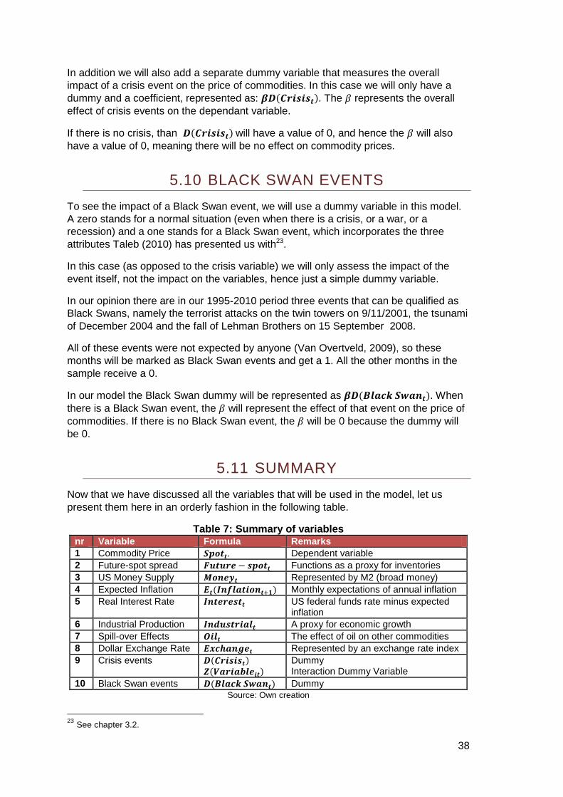
38

In addition we will also add a separate dummy variable that measures the overall impact of a crisis event on the price of commodities. In this case we will only have a dummy and a coefficient, represented as: �=��0-1-1��. The # represents the overall effect of crisis events on the dependant variable.

If there is no crisis, than =��0-1-1��will have a value of 0, and hence the # will also have a value of 0, meaning there will be no effect on commodity prices.

5.10 BLACK SWAN EVENTS

To see the impact of a Black Swan event, we will use a dummy variable in this model. A zero stands for a normal situation (even when there is a crisis, or a war, or a recession) and a one stands for a Black Swan event, which incorporates the three attributes Taleb (2010) has presented us with23.

In this case (as opposed to the crisis variable) we will only assess the impact of the event itself, not the impact on the variables, hence just a simple dummy variable.

In our opinion there are in our 1995-2010 period three events that can be qualified as Black Swans, namely the terrorist attacks on the twin towers on 9/11/2001, the tsunami of December 2004 and the fall of Lehman Brothers on 15 September 2008.

All of these events were not expected by anyone (Van Overtveld, 2009), so these months will be marked as Black Swan events and get a 1. All the other months in the sample receive a 0.

In our model the Black Swan dummy will be represented as �=�B+,6C�D,%��. When there is a Black Swan event, the # will represent the effect of that event on the price of commodities. If there is no Black Swan event, the # will be 0 because the dummy will be 0.

5.11 SUMMARY

Now that we have discussed all the variables that will be used in the model, let us present them here in an orderly fashion in the following table.

Table 7: Summary of variables nr Variable Formula Remarks 1 Commodity Price ��. Dependent variable 2 Future-spot spread �3�30& − 1�� Functions as a proxy for inventories 3 US Money Supply $�%&'� Represented by M2 (broad money) 4 Expected Inflation (��)%*+,�-�%�./� Monthly expectations of annual inflation 5 Real Interest Rate )%�&0&1�� US federal funds rate minus expected

inflation 6 Industrial Production )%231�0-,+� A proxy for economic growth 7 Spill-over Effects 4-+� The effect of oil on other commodities 8 Dollar Exchange Rate (567,%8&� Represented by an exchange rate index 9 Crisis events =��0-1-1��

?�@,0-,A+&-�� Dummy Interaction Dummy Variable

10 Black Swan events =�B+,6C�D,%�� Dummy Source: Own creation

23 See chapter 3.2.

39

6. THE MODEL

6.1 THE BASIC MODEL

If we bring all these variables together we get the following basic model:

�!"�� = 9 + #E�� − !"�� + #E<F�� − !"�� + #G�H:;�� + #G<F�H:;��

+ #I EK�LMN;O�:"M�.E� + #I<FPQ��LMN;O�:"M�.E�R + #S�LM�� O��

+ #S<F�LM�� + #T�LMU� ��:O;�� + #T<F�LMU� ��:O;�� + #V�W"M�X��

+#V<F�W"M�X�� + #Y�QZℎOM\�� + #Y

<F�QZ]ℎOM\�� + #^_��: : ��+ #`_�a;O]b�cOM�� + >�

Although this basic form looks good on first sight there are some issues with it which we need to resolve before we can move on to the discussion of the descriptive statistics and the regressions.

6.2 TRANSFORMATIONS

In this chapter we will discuss (and perform) the various transformations that are necessary to get this model econometrically correct and to make it as easy as possible to interpret the results of the regressions.

6.2.1 LOGARITMS

The reason we take logarithms is because when the first differences24 of logarithms are taken and the regression is estimated the # can be interpreted as follow: When the explanatory variable rises by one percent, then the dependent variable will change by X percent, i.e. the # will be a measure of elasticity (Koop, 2006).

Unfortunately, the very nature of some of our variables makes it difficult (or even impossible) to take logs of them. In the following table we will present all our variables, with an indication if logs are possible. When not, we will give an explanation for this. The dummy variables are excluded because it has no use to take logs of them.

Table 8: Overview of logaritms Variable Log or not ��. Log �3�30& − 1�� No log $�%&'� Log (��)%*+,�-�%�./� No log )%�&0&1�� No log )%231�0-,+� Log 4-+� Log (567,%8&� Log

Source: Own creation

As we can see, there are three variables where we won’t take the logarithms. These are the Inventory, Inflation and Interest variables.

24 See 6.2.2 for the explanation about the first differences.

40

In the case of the Interest and Inflation variables the explanation lies within their very nature, since these variables are already measured in percentages .

When taking the first differences of them (later on), this will automatically result in a percentage change. Thus it is not necessary to take logs, since that would only make it more complicated to interpret the influence of these variables on the prices of commodities (i.e. the percentage change of a percentage change).

The future-spot spread-variable has a more mathematical reason why taking logs isn’t possible. As previously mentioned this variable is made up out of the future-spot spread as a proxy for inventories . Since this spread is negative (all the time) it is impossible to take logarithms of this variable. Hence we leave it in its original state.

Interpretation wise this won’t have much impact, just that we can’t say that a change of one percent in the inventories/future-spot spread has an impact of X percent on the spot price. The interpretation will be more like: A change of the future-spot spread by 1 unit, will result in a percentage change of X % of the Spot price. But more on this in the chapter on the interpretation of the regression results.

6.2.2 FIRST DIFFERENCES (UNIT ROOT TESTING)

In their current state we suspect that most (or all) of our variables are non-stationary . Econometrically it will give problems when we would regress non-stationary variables onto each other. This might result in spurious regressions, meaning that the results might be misleading and incorrect (Koop, 2006).

Before we continue, we will perform unit root tests on our variables to see whether they are stationary or not. For this we use the augmented Dickey-Fuller test. When the P-value given by this test is greater than 0.05, then the tested variable has a unit root and thus is non-stationary. We get the following results25.

Table 9: Augmented Dickey-Fuller test results Variable Dicky -Fuller P -value

(constant) d%��. 0,8495 �3�30& − 1�� 0,702 d%�$�%&'�� 0,7913 (��)%*+,�-�%�./� 0,0939 )%�&0&1�� 0,8121 d%�)%231�0-,+�� 5,788e-026 d%�4-+�� 0,7863 d%�(567,%8&�� 0,3655

Source: own calculations

As we can see all the series, except for the industrial production, have P-values that are higher than 0,05. Luckily for us there is an easy solution to this problem: We can transform these non-stationary variables into stationary variables by taking the first differences.

25 We will make changes to the interaction dummy variables afterward, depending on the results of the Dicky-Fuller test on the variables they are based on. They will not be added to this test.

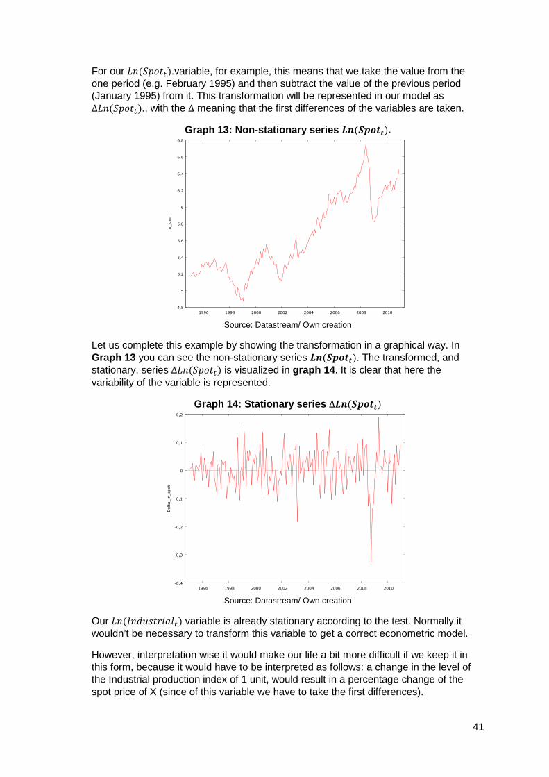
41

For our eM��!"��.variable, for example, this means that we take the value from the one period (e.g. February 1995) and then subtract the value of the previous period (January 1995) from it. This transformation will be represented in our model as ∆eM��!"��., with the ∆ meaning that the first differences of the variables are taken.

Graph 13: Non-stationary series d%��.

Source: Datastream/ Own creation

Let us complete this example by showing the transformation in a graphical way. In Graph 13 you can see the non-stationary series d%��. The transformed, and stationary, series ∆eM��!"�� is visualized in graph 14 . It is clear that here the variability of the variable is represented.

Graph 14: Stationary series ∆d%��

Source: Datastream/ Own creation

Our eM�LMU� ��:O;�� variable is already stationary according to the test. Normally it wouldn’t be necessary to transform this variable to get a correct econometric model.

However, interpretation wise it would make our life a bit more difficult if we keep it in this form, because it would have to be interpreted as follows: a change in the level of the Industrial production index of 1 unit, would result in a percentage change of the spot price of X (since of this variable we have to take the first differences).

4,8

5

5,2

5,4

5,6

5,8

6

6,2

6,4

6,6

6,8

1996 1998 2000 2002 2004 2006 2008 2010

Ln_spot

-0,4

-0,3

-0,2

-0,1

0

0,1

0,2

1996 1998 2000 2002 2004 2006 2008 2010

Delta_ln

_spot

42

So, we also will take the first differences of the Ln(IndustrialK) in order be able to interpret our model in a concise and easy fashion.

Now, before we move on to the formal presentation of the model, let us do one final Augmented Dickey-Fuller test to show that all our variables are now stationary and ready to be used in our regressions. The results of this test are in the table below.

Table 10: Augmented Dickey-Fuller test results for the first differences of the variables

Variable Dicky -Fuller P -value (constant)

∆d%(��). 3,018e-016 ∆�3�30& − 1�� 1,77e-012 ∆d%($�%&'�) 8,767e-013 ∆(�()%*+,�-�%�./) 1,69e-018 ∆)%�&0&1�� 4,757e-032 ∆d%()%231�0-,+�) 3,05e-020 ∆d%(4-+�) 4,189e-017 ∆d%((567,%8&�) 2,893e-016


And indeed, all p-values are now smaller than 0,05, meaning that all series are now stationary.

6.2.3 CO-INTEGRATION RELATIONS

After the unit-root testing we know that our untransformed variables are non-stationary (except for industrial production), as presented in table 11 . Non-stationary variables might also imply co-integration26.

When we do the Johansen test for co integration on our basic variables (being d%(��), �3�30& − 1��, d%($�%&'�) and so on, excluding any dummy variables or interaction dummies), we see that there are six co integration relations. This is represented in the following table with the Johansen test results.

It is interesting to note that Roache and Erbil (2010) also found co-integration relations between their variables (inventories, base metal spot prices, futures prices and interest rates).

Table 11: Johansen test for co-integration Rank Trace test Lmax 0 339,89 [0,0000] 91,973 [0,0000] 1 247,91 [0,0000] 73,879 [0,0000] 2 174,04 [0,0000] 64,969 [0,0000] 3 109,07 [0,0000] 43,444 [0,0015] 4 65,622 [0,0003] 32,132 [0,0095] 5 33,491 [0,0171] 23,823 [0,0182] 6 9,6680 [0,3128] 6,2772 [0,5849] 7 3,3908 [0,0656] 3,3908 [0,0656]

Source: Statistics program/ Own creation

26 When X and Y (independent and dependent variables) are non-stationary, their error terms have a stochastic trend. When variables are co-integrated, the errors do not have a trend (which means that the trends of X and Y will cancel each other out). The error will not get too large and X and Y will not diverge from one another. They will, in essence, trend together. When co-integration is present, this might imply that there is an equilibrium relation between the two variables, with the error term as the equilibrium error (Koop, 2006)

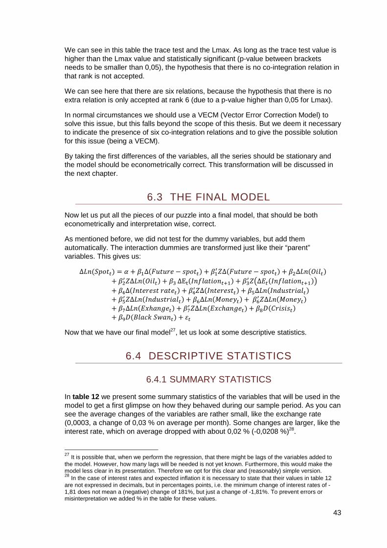
43

We can see in this table the trace test and the Lmax. As long as the trace test value is higher than the Lmax value and statistically significant (p-value between brackets needs to be smaller than 0,05), the hypothesis that there is no co-integration relation in that rank is not accepted.

We can see here that there are six relations, because the hypothesis that there is no extra relation is only accepted at rank 6 (due to a p-value higher than 0,05 for Lmax).

In normal circumstances we should use a VECM (Vector Error Correction Model) to solve this issue, but this falls beyond the scope of this thesis. But we deem it necessary to indicate the presence of six co-integration relations and to give the possible solution for this issue (being a VECM).

By taking the first differences of the variables, all the series should be stationary and the model should be econometrically correct. This transformation will be discussed in the next chapter.

6.3 THE FINAL MODEL

Now let us put all the pieces of our puzzle into a final model, that should be both econometrically and interpretation wise, correct.

As mentioned before, we did not test for the dummy variables, but add them automatically. The interaction dummies are transformed just like their “parent” variables. This gives us:

∆eM(�!"��) = 9 + #E∆(�� − !"��) + #E<F∆(�� − !"��) + #G∆eM(H:;�)

+ #G< F∆eM(H:;�) + #I ∆EK(LMN;O�:"M�.E) + #I

< FP∆Q�(LMN;O�:"M�.E)R+ #S∆(LM�� O�� + #S<F∆�LM�� + #T∆eM�LMU� ��:O;��+ #T

<F∆eM�LMU� ��:O;�� + #V∆eM�W"M�X�� +#V<F∆eM�W"M�X��

+ #Y∆eM�QZℎOM\�� + #Y<F∆eM�QZ]ℎOM\�� + #^_��: : ��

+ #`_�a;O]b�cOM�� + >�

Now that we have our final model27, let us look at some descriptive statistics.

6.4 DESCRIPTIVE STATISTICS

6.4.1 SUMMARY STATISTICS

In table 12 we present some summary statistics of the variables that will be used in the model to get a first glimpse on how they behaved during our sample period. As you can see the average changes of the variables are rather small, like the exchange rate (0,0003, a change of 0,03 % on average per month). Some changes are larger, like the interest rate, which on average dropped with about 0,02 % (-0,0208 %)28.

27 It is possible that, when we perform the regression, that there might be lags of the variables added to the model. However, how many lags will be needed is not yet known. Furthermore, this would make the model less clear in its presentation. Therefore we opt for this clear and (reasonably) simple version. 28 In the case of interest rates and expected inflation it is necessary to state that their values in table 12 are not expressed in decimals, but in percentages points, i.e. the minimum change of interest rates of -1,81 does not mean a (negative) change of 181%, but just a change of -1,81%. To prevent errors or misinterpretation we added % in the table for these values.

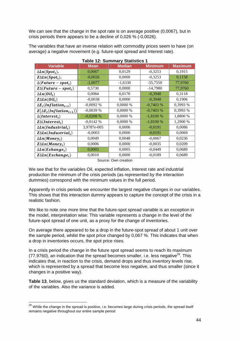
44

We can see that the change in the spot rate is on average positive (0,0067), but in crisis periods there appears to be a decline of 0,026 % (-0,0026).

The variables that have an inverse relation with commodity prices seem to have (on average) a negative movement (e.g. future-spot spread and Interest rate).

Table 12: Summary Statistics 1 Variable Mean Median Minimum Maximum

∆d%(��). 0,0067 0,0129 -0,3253 0,1915

?∆d%(��). -0,0026 0,0000 -0,3253 0,1158

∆(�3�30& − 1��) -1,0077 -1,6330 -35,7550 77,9760

?∆(�3�30& − 1��) 0,5730 0,0000 -14,7980 77,9760

∆d%(4-+�) 0,0084 0,0170 -0,3948 0,3118

?∆d%(4-+�) -0,0038 0,0000 -0,3948 0,1906

∆(�()%*+,�-�%�./) -0,0092 % 0,0000 % -0,7403 % 0,3993 %

?P∆(�()%*+,�-�%�./)R -0,0039 % 0,0000 % -0,7403 % 0,3993 %

∆()%�&0&1��) -0,0208 % 0,0000 % -1,8100 % 1,8800 %

?∆()%�&0&1��) -0,0142 % 0,0000 % -1,8100 % 1,2900 %

∆d%()%231�0-,+�) 3,9787e-005 0,0006 -0,0191 0,0086

?∆d%()%231�0-,+�) -0,0003 0,0000 -0,0191 0,0069

∆d%($�%&'�) 0,0049 0,0048 -0,0067 0,0236

?∆d%($�%&'�) 0,0006 0,0000 -0,0035 0,0209

∆d%((57,%8&�) 0,0003 0,0005 -0,0449 0,0689

?∆d%((567,%8&�) 0,0010 0,0000 -0,0189 0,0689 Source: Own creation

We see that for the variables Oil, expected inflation, Interest rate and industrial production the minimum of the crisis periods (as represented by the interaction dummies) correspond with the minimum values in the full period.

Apparently in crisis periods we encounter the largest negative changes in our variables. This shows that this interaction dummy appears to capture the concept of the crisis in a realistic fashion.

We like to note one more time that the future-spot spread variable is an exception in the model, interpretation wise: This variable represents a change in the level of the future-spot spread of one unit, as a proxy for the change of inventories.

On average there appeared to be a drop in the future-spot spread of about 1 unit over the sample period, whilst the spot price changed by 0,067 %. This indicates that when a drop in inventories occurs, the spot price rises.

In a crisis period the change in the future spot spread seems to reach its maximum (77,9760), an indication that the spread becomes smaller, i.e. less negative29. This indicates that, in reaction to the crisis, demand drops and thus inventory levels rise, which is represented by a spread that become less negative, and thus smaller (since it changes in a positive way).

Table 13 , below, gives us the standard deviation, which is a measure of the variability of the variables. Also the variance is added.

29 While the change in the spread is positive, i.e. becomes large during crisis periods, the spread itself remains negative throughout our entire sample period

45

Table 13: Summary Statistics 2 Variable Std. Dev. C.V. ∆d%(��). 0,0663 9,9027

?∆d%(��). 0,0312 12,201

∆(�3�30& − 1��) 12,9952 12,8966

?∆(�3�30& − 1��) 6,7149 11,7199

∆d%(4-+�) 0,0957 11,4060

?∆d%(4-+�) 0,0409 10,8478

∆(�()%*+,�-�%�./) 0,1137 12,3660

?P∆(�()%*+,�-�%�./)R 0,06381 16,5158

?∆()%�&0&1��) 0,2269 15,9768

∆d%()%231�0-,+�) 0,0041 103,231

?∆d%()%231�0-,+�) 0,0024 14,3684

∆d%($�%&'�) 0,0037 0,7594

?∆d%($�%&'�) 0,0026 4,3554

∆d%((57,%8&�) 0,0149 54,8523

?∆d%((567,%8&�) 0,0066 6,81532 Source: Own creation

6.4.2 XY-PLOTS AND CORRELATION

In this chapter we will look a bit closer into the interactions between the dependant and the independent variables by means of the XY-plots and the correlation between these variables. We will discuss the XY-plots and correlations between the main variables30.

On graph 15 we can clearly see that there is a strong negative correlation (-0,9234) between the changes in the spot price (%) and the changes in the future-spot spread. This indicates that a rise in the future spot spread will result in a % drop of the spot price. Or otherwise stated: when commodity inventories rise, as indicated by a rise of the future spot spread (i.e. the spread becomes less negative) then the spot price will drop (% wise).

Graph 15: XY-plot ∆d%(��).vs ∆(�3�30& − 1��)


30 We focus here on the main variables to give a first view of their relation with the dependant variable.

-40

-20

0

20

40

60

80

-0,3 -0,2 -0,1 0 0,1 0,2

Delta_fu

ture

_sp

Delta_ln_spot

Delta_future_sp versus Delta_ln_spot (with least squares fit)

Y = 0,204 - 181,X

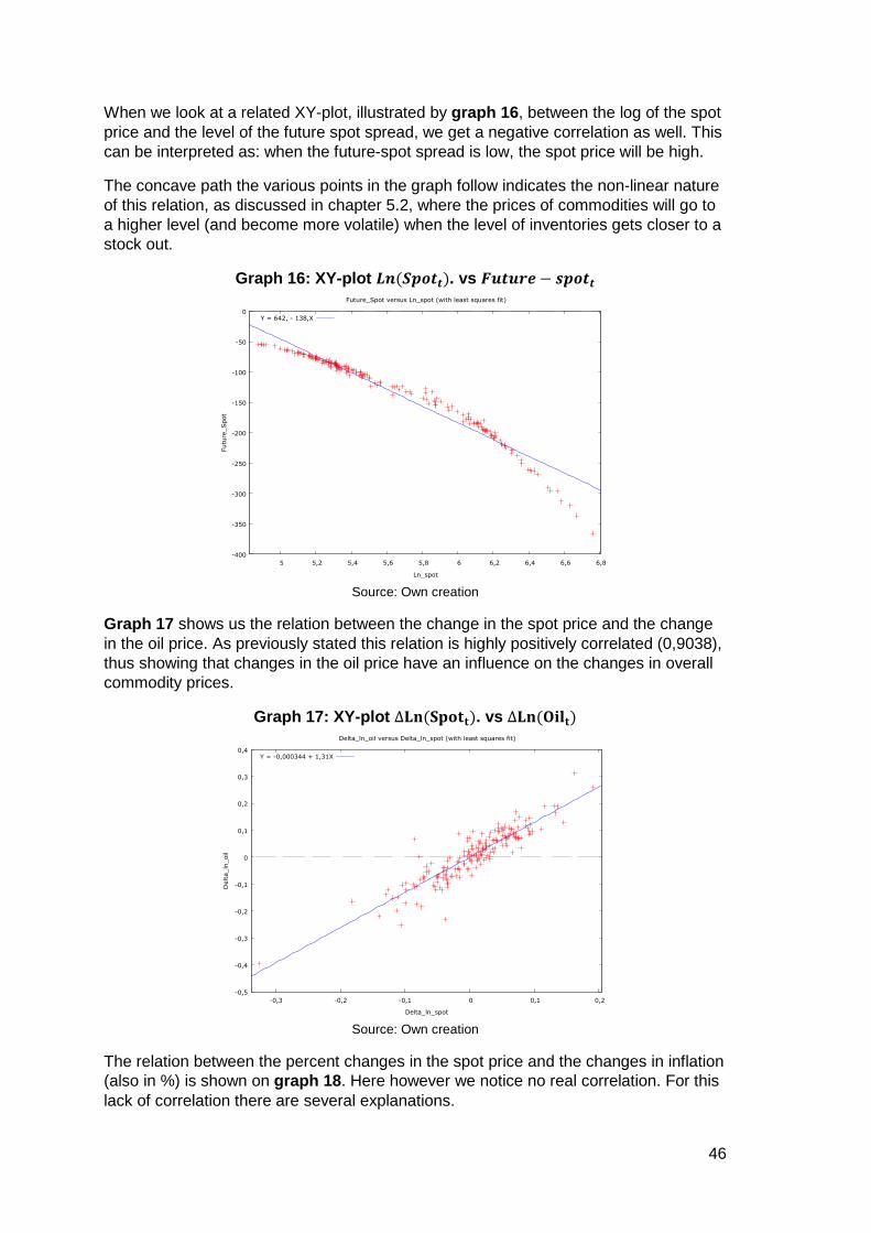
46

When we look at a related XY-plot, illustrated by graph 16 , between the log of the spot price and the level of the future spot spread, we get a negative correlation as well. This can be interpreted as: when the future-spot spread is low, the spot price will be high.

The concave path the various points in the graph follow indicates the non-linear nature of this relation, as discussed in chapter 5.2, where the prices of commodities will go to a higher level (and become more volatile) when the level of inventories gets closer to a stock out.

Graph 16: XY-plot d%(��). vs �3�30& − 1��


Graph 17 shows us the relation between the change in the spot price and the change in the oil price. As previously stated this relation is highly positively correlated (0,9038), thus showing that changes in the oil price have an influence on the changes in overall commodity prices.

Graph 17: XY-plot ∆st(uvwxx). vs ∆st(yz{x)


The relation between the percent changes in the spot price and the changes in inflation (also in %) is shown on graph 18 . Here however we notice no real correlation. For this lack of correlation there are several explanations.

-400

-350

-300

-250

-200

-150

-100

-50

0

5 5,2 5,4 5,6 5,8 6 6,2 6,4 6,6 6,8

Futu

re_Spot

Ln_spot

Future_Spot versus Ln_spot (with least squares fit)

Y = 642, - 138,X

-0,5

-0,4

-0,3

-0,2

-0,1

0

0,1

0,2

0,3

0,4

-0,3 -0,2 -0,1 0 0,1 0,2

Delta_ln

_oil

Delta_ln_spot

Delta_ln_oil versus Delta_ln_spot (with least squares fit)

Y = -0,000344 + 1,31X

47

It might be due to the fact that the data on this variable was obtained on a quarterly basis and then transformed into monthly data31. Because of this though, we have for 3/4th of the time a change of zero in expected inflation in our sample period.

A second explanation, more economically in nature, is that there is no relation between expected inflation and commodity prices. Higher commodity prices might cause higher inflation expectations, but this might take some time (also because the survey is taken on a quarterly basis).

It is also very plausible that commodity prices cause expected inflation and not the other way around32, since expected inflation will rise when people see that commodity prices are high.

If we look at the correlation, we see there is a very small positive correlation of 0,0979.

Graph 18: XY-plot ∆st(uvwxx). vs ∆|x(}t~{�xzwtx./)


Because of this lack of correlation, due to the unavailability of monthly expected inflation data, it is likely that the expected inflation variable might be excluded from the model when performing the OLS-regression.

In graph 19 we present the relation between the spot price and expected inflation to see if there exists a relation when working solely with the levels (and not first differences), where we can see a negative correlation between the two variables.

This is surprising since rising commodity prices should result in rising expected inflation, or rising inflation should result in a rise of commodity prices (correlation tells nothing about causality), but not a drop.

The observations are very scattered though, so the relation is not very strong. Maybe there is a negative relation when spot prices are low, and a positive relation when spot prices are high? Or maybe spot price levels in general have a negative impact on expected inflation? 31 See chapter 5.4 32 We like to add that our VAR model might shed some light on this when we investigate the Granger Causality. Furthermore we investigate expected inflation (expectations of people) and not inflation itself, which is calculated based on actual changes in the CPI and is only known quite some time after the events (i.e. change in commodity price took place).

-0,8

-0,6

-0,4

-0,2

0

0,2

0,4

-0,3 -0,2 -0,1 0 0,1 0,2

delta_In

flation

Delta_ln_spot

48

This might be revealed by an OLS regression, but due to econometric factors (non-stationarity) we will not be able to delve deeper into this.

Graph 19: XY-plot st(uvwxx) vs |x(}t~{�xzwtx./)


In graph 20 we can see the correlation between the change in the spot price and the change in real interest rates. Here also we can see that there is no correlation to be found. This is due to the fact that changes in the interest rate are very small (central banks commonly rise or drop the rate with no more than 0,25% each quarter).

Also the creation of this variable is linked with the expected inflation variable and thus biased by the data difficulties that messed with our inflation variable. There appears to be no correlation between the ∆Ln(SpotK) and EK(InflationK.E) as well. If we look at the correlation matrix we see, however, that there is a small positive correlation of 0,1176.

Graph 20: XY-plot ∆st�uvwxx� vs ∆�}tx��xx�


1,6

1,8

2

2,2

2,4

2,6

2,8

3

3,2

3,4

3,6

5 5,2 5,4 5,6 5,8 6 6,2 6,4 6,6 6,8

Inflation

Ln_spot

Inflation versus Ln_spot (with least squares fit)

Y = 4,66 - 0,393X

-2

-1,5

-1

-0,5

0

0,5

1

1,5

2

-0,3 -0,2 -0,1 0 0,1 0,2

Delta_In

tere

st

Delta_ln_spot

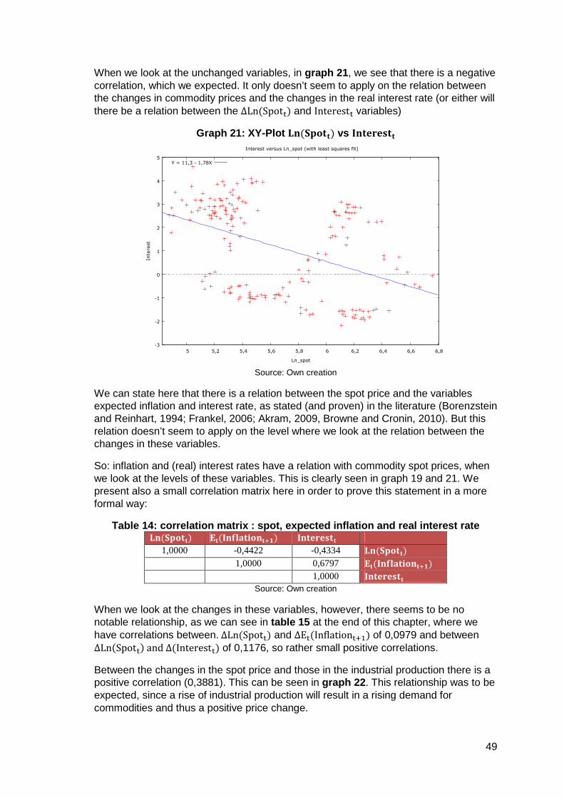
49

When we look at the unchanged variables, in graph 21 , we see that there is a negative correlation, which we expected. It only doesn’t seem to apply on the relation between the changes in commodity prices and the changes in the real interest rate (or either will there be a relation between the ∆Ln(SpotK) and InterestK variables)

Graph 21: XY-Plot st(uvwxx) vs }tx��xx


We can state here that there is a relation between the spot price and the variables expected inflation and interest rate, as stated (and proven) in the literature (Borenzstein and Reinhart, 1994; Frankel, 2006; Akram, 2009, Browne and Cronin, 2010). But this relation doesn’t seem to apply on the level where we look at the relation between the changes in these variables.

So: inflation and (real) interest rates have a relation with commodity spot prices, when we look at the levels of these variables. This is clearly seen in graph 19 and 21. We present also a small correlation matrix here in order to prove this statement in a more formal way:

Table 14: correlation matrix : spot, expected infla tion and real interest rate st(uvwxx) |x(}t~{�xzwtx./) }tx��xx

1,0000 -0,4422 -0,4334 st(uvwxx) 1,0000 0,6797 |x(}t~{�xzwtx./) 1,0000 }tx��xx


When we look at the changes in these variables, however, there seems to be no notable relationship, as we can see in table 15 at the end of this chapter, where we have correlations between.∆Ln�SpotK� and ∆EK�InflationK.E� of 0,0979 and between ∆Ln�SpotK�and∆�InterestK� of 0,1176, so rather small positive correlations.

Between the changes in the spot price and those in the industrial production there is a positive correlation (0,3881). This can be seen in graph 22 . This relationship was to be expected, since a rise of industrial production will result in a rising demand for commodities and thus a positive price change.

-3

-2

-1

0

1

2

3

4

5

5 5,2 5,4 5,6 5,8 6 6,2 6,4 6,6 6,8

Inte

rest

Ln_spot

Interest versus Ln_spot (with least squares fit)

Y = 11,3 - 1,78X

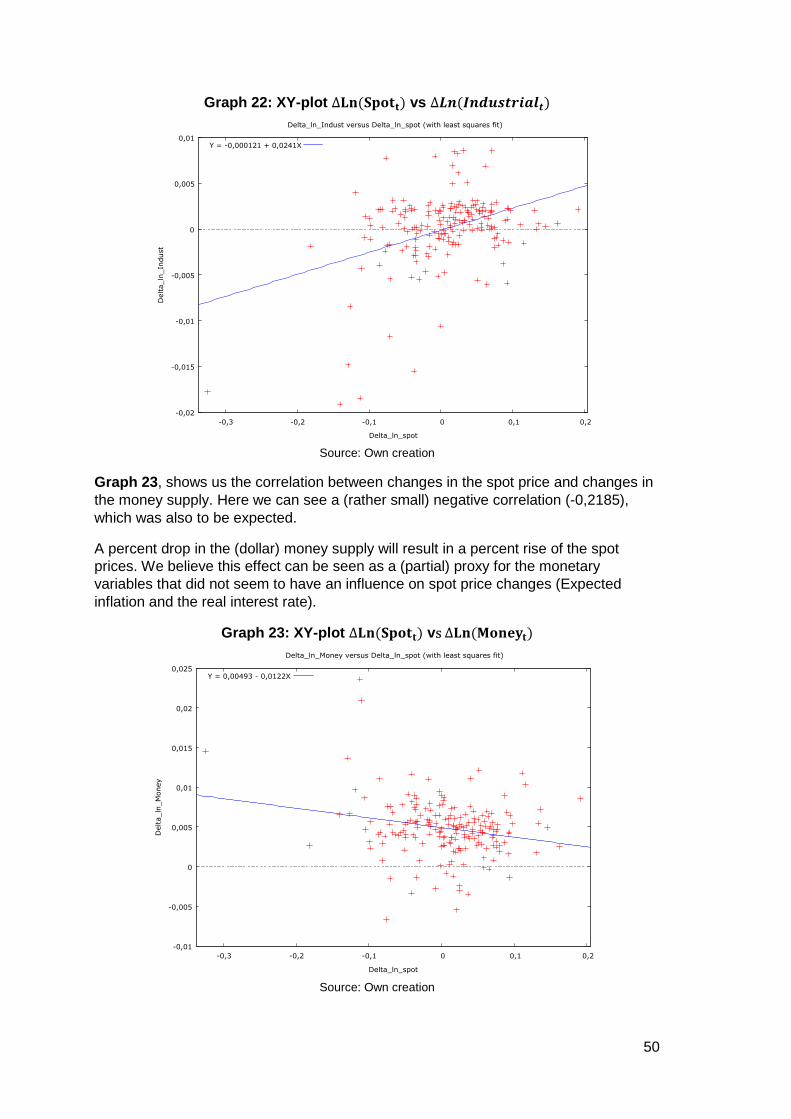
50

Graph 22: XY-plot ∆st(uvwxx) vs ∆d%()%231�0-,+�)


Graph 23 , shows us the correlation between changes in the spot price and changes in the money supply. Here we can see a (rather small) negative correlation (-0,2185), which was also to be expected.

A percent drop in the (dollar) money supply will result in a percent rise of the spot prices. We believe this effect can be seen as a (partial) proxy for the monetary variables that did not seem to have an influence on spot price changes (Expected inflation and the real interest rate).

Graph 23: XY-plot ∆st(uvwxx) vs ∆st(�wt��x)


-0,02

-0,015

-0,01

-0,005

0

0,005

0,01

-0,3 -0,2 -0,1 0 0,1 0,2

Delta_ln

_In

dust

Delta_ln_spot

Delta_ln_Indust versus Delta_ln_spot (with least squares fit)

Y = -0,000121 + 0,0241X

-0,01

-0,005

0

0,005

0,01

0,015

0,02

0,025

-0,3 -0,2 -0,1 0 0,1 0,2

Delta_ln

_M

oney

Delta_ln_spot

Delta_ln_Money versus Delta_ln_spot (with least squares fit)

Y = 0,00493 - 0,0122X

51

And last, but not least; we arrive at graph 24 , which shows us the relation between changes in the spot price and changes in the (dollar) exchange rate. As expected the correlation is negative (-0,4245), meaning that a percent rise of the dollar exchange rate (index) will result in a percent drop of commodity prices.

Graph 24: XY-plot ∆d%(��) vs ∆d%((567,%8&�)


Before moving on to the OLS-regression and the final answers to our research questions, we present here the correlation matrix to give an overview of the relations of the variables with the dependant variable and with each other.

Table 15: Correlation matrix: Main variables Spot

Price

Future

spot

spread

Crude Oil Expected

Inflation

Real

Interest

Rate

Industrial

production

Money

Supply

Exchange

Rate

Spot Price 1

Future Spot

Spread

-0,9234 1

Crude Oil 0,9038 -0,7807 1

Expected

Inflation

0,0979 -0,0996 0,1578 1

Real Interest

Rate

0,1176 -0,0944 0,1215 -0,2167 1

Industrial

Production

0,3881 -0,4105 0,3357 0,1859 0,1070 1

Money

Supply

-0,2185 0,2040 -0,2284 -0,0943 -0,1885 -0,4316 1

Exchange

Rate

-0,4245 0,4459 -0,3367 -0,0738 -0,0072 -0,2704 0.0902 1


-0,06

-0,04

-0,02

0

0,02

0,04

0,06

0,08

-0,3 -0,2 -0,1 0 0,1 0,2

Delta_ln

_Exchan

Delta_ln_spot

Delta_ln_Exchan versus Delta_ln_spot (with least squares fit)

Y = 0,000908 - 0,0952X

52

7. THE UNIVARIATE MODEL: OLS-REGRESSION

7.1 OLS-REGRESSIONS AND TESTS

To what extent do several determinants have an impa ct on the price evolutions of commodities?

To answer this question we will perform a series of OLS regressions, starting with a regression on our basic model, i.e. on the levels of the variables. Once this is done we move on to a series of regression that will be performed on our transformed variables.

The results of these regressions will be interpreted and at the end of this chapter, we will select the regression which gives us the best results, both econometrically as well as economically.

7.2 PRELUDE: OLS ON LEVELS

Before we move on, let us first estimate our model without any of the previously discussed transformations. In the following table we give the results of this regression:

Table 16: Ols-regression results: Levels Variable Coefficient Variable Coefficient � 58,8016

(1,64) =(B+,6C�D,%�� -3,9501

(-0,79) ��3�30& − 1�� -1,2605

(-16,13) ?��3�30&− 1��

0,0792 (0,17)

�4-+�� 0,411845 (12,49)

?�4-+�� 0,0599 (0,29)

|x�)%*+,�-�%�./� 2,3336 (0,95)

?P(��)%*+,�-�%�./� -15,1898 (-1,04)

�)%�&0&1�0,�&�� 3,2792 (6,73)

?�)%�&0&1�� -4,7526 (-1,16)

�)%231�0-,+�� -0,2209 (-0,58)

?�)%231�0-,+�� -0,3550 (-0,14)

�$�%&'�� 0,0108 (9,56)

?�$�%&'�� -0,0121 (-1,26)

�(57,%8&�� -0,5537 (-7,42)

?�(567,%8&�� -0,0887 (-0,24)

=��0-1-1�� 155,979 (0,64)

R² Durbin Watson

0,9985 0,5304


As we have anticipated we have high t-ratios (between brackets) for our significant coefficients, a very high R² and a low Durbin Watson, which all points in the direction of spurious regression.

53

7.3 BASIC REGRESSION: FIRST DIFFERENCES

Table 17 shows us the estimation results for the model using first differences, including all the variables. The ∆(�� − !"��) and ∆eM(H:;�) variables appear to be highly significant (i.e. they have very high t-ratios, namely -17,19 and 15,27 respectively). The future-spot crisis interaction dummy and the interest rate crisis interaction dummy also seem to have a significant impact on the commodity spot prices.

Furthermore this OLS regression has an R² of 0,945977, which implies that more than 94 % of changes in commodity spot prices is mainly explained by the two variables ∆(�� − !"��) and ∆eM(H:;�), due to their high significance. This, however, seems unlikely to us.

We believe these two variables, due to their very high correlation with the dependant variable, disturb the output of the model.

This is might certainly be the case for the future-spot spread , since this variable is made up from the difference between the future price (3 month future) and the spot price and is thus automatically highly correlated with its “parent” variable. This might result in a biased coefficient.

However, as we have stated when discussing the future-spot spread and its value as a proxy for inventories, we deem it possible that this variable, together with the change in the oil price, could have such a significant impact on commodity prices and might be capable of explaining such a large percentage of the price changes of commodity spot prices.

The oil price on the other hand, is a less clear case. It is not surprising that the oil price explains a lot of commodity prices, since it takes up such a big part of the production (and transportation) costs. So, the high explanatory power of the oil price might just indicate that it has a large impact on commodity price changes and is not an econometric problem.

However, since our dependent variable is made up out of the GSCI, of which 66,5 % is made up from energy commodities, there is automatically a high correlation between the oil and spot price variable, which might cause some econometric problems.

Because of this unclear view whether oil and the future-spot spread really disturb our coefficients (or are correct coefficients), we do not dismiss these variables immediately, but we opt to take two paths here.

We will on one hand discuss the OLS regression output, including these R²-inflating variables and on the other hand we will also discuss a regression output without ∆(�� − !"��) and ∆eM(H:;�), in chapter 7.4. This in order to keep an objective view and interpret both possibilities in their full extent.

As you can see, we have 4 significant coefficients, as mentioned before. The high t-ratios and the high R² might indicate spurious regression, but due to the fact that we took first differences of the variables, this is unlikely. The Durbin Watson test statistic of 2,0813 indicates that there is no residual autocorrelation.

54

Table 17: OLS-Regression results: First differences with oil and future-spot Variable Coefficient Variable Coefficient � 6,26e-05

(0,03) ∆d%()%231�0-,+�) 0,2476

(0,63) ∆(�3�30&− 1��)

-0,0029 (-17,19)

?∆d%()%231�0-,+�) -1,7414 (-1,23)

Z∆(�3�30& −1��)

0,0004 (0,66)

∆d%($�%&'�) 0,1434 (0,35)

∆d%(4-+�) 0,3171 (15,27)

?∆d%($�%&'�) -1,1409 (-1,13)

?∆d%(4-+�) 0,2203 (2,48)

∆d%((57,%8&�) -0,1835 (-1,93)

∆|x()%*+,�-�%�./) -0,0162 (-1,26)

?∆d%((567,%8&�) 0,7917 (1,76)

?P∆(�()%*+,�-�%�./ -0,0187 (-0,57)

=(�0-1-1�) 0,0044 (0,63)

∆()%�&0&1�0,�&�� 0,0035 (1,30)

=�B+,6C�D,%�� -0,0089 (-0,71)

?∆�)%�&0&1�� -0,0170 (-2,18)

R² Durbin Watson

0,9460 2,0813


We can interpret the coefficients as follows:

A change of 1 unit of the future-spot spread , ceteris paribus, will be reflected33 by a negative change of the spot price of 0,0029 %. This is in line with the theory we presented in chapter 5.2.

When commodity inventories (as represented by the future-spot spread) rise, the spot price will drop. These results give us an indication, that, viewed over our entire sample period, inventories have risen, since the effect on the price is negative34. This is also in line with findings in the literature (IMF, 2008), although our coefficient is rather small.

A change in the oil price of 1%, ceteris paribus, will be met by a change of the commodity spot prices of 0,317 %. This might reflect the impact of oil prices on the production costs of commodities (spill-over effect). If we link this result to the literature (Baffes, 2007), we see that our coefficient is quite a bit higher than the 0,16 that Baffes found for the impact of the oil price on a commodity index.

The fact that our coefficient is twice as big can be put into perspective though. Baffes (2007) used a non-energy commodity index as dependent variable, which already might have an impact on the size and significance of the coefficient (since in his case, the correlation between oil and the index will be much lower).

Secondly, the research period ranged from 1960-2005, a period in which, most of the time; the oil price was very low. The really high prices are a recent phenomenon, and have a serious impact on our coefficient. Also, our research period is much shorter, so volatility can be higher during our sample period.

33 A regression does not tell us much about the causality. It could be that the change in the future spot spread causes the spot price to change, but the opposite is also possible. 34 Unfortunately the inverse leverage effect between commodity prices and inventories is not shown in these results. As inventories come closer to a stock-out, i.e. the future-spot spread becomes wider (and more negative) the impact on the prices should become larger (prices become more volatile). When inventories rise (like seems to be the case here) the spot price will react less severe than when there should have been drops in inventory levels (over the entire period).

55

When there is a crisis, a rise of the oil price of 1% ,ceteris paribus, there will be an extra commodity spot price rise of 0,22%, as shown by the Z∆Ln(OilK) interaction dummy.

So, in times of crisis, the oil price will have a higher impact on commodity prices than in normal circumstances and a 1% change in oil price will result in a total change of spot prices of 0,53 %. When we enter a crisis period, volatility of prices will rise. Hence, the impact of a chance in the oil price will be larger.

Bhar and Hammoudeh (2010) state that during a high variance state (i.e. a crisis period, when volatility is high), which is associated with economic uncertainty and inflationary shocks, that in turn cause higher interest rates and a dollar depreciation there will a flight to the safety of currency commodities such as oil in response to a weakening dollar. If demand for oil rises, then its price rises and its impact on commodity prices increases.

The crisis interaction dummy �∆(}tx��xx), with a coefficient of -0,017, shows that during a crisis period, a rise of the interest rate with 1 %, ceteris paribus, will be met by a drop of the spot price of 0,017%.

This might indicate a flight to safety when confronted with rising interest rates during a crisis period. In this case, when interest rates rise by 1 %, an investment in government bonds (for example) becomes more interesting than an investment in (volatile) commodities. Investors will sell their commodities (prices drop) and buy bonds.

The opposite will be true as well: A drop of interest rates of 1 % results in a price rise of commodities by 0,017 %. When central banks try to counter the effects of the crisis by lowering interest rates (as they did in 2008), bonds will become less attractive and investors start “looking for yield” and buy commodities.

This is also in line with the results of Anzuini, Lombardi and Pagano (2010) , which showed that (for the impact of monetary policy on oil futures) a positive monetary policy shock (in their case a tightening of monetary policy, i.e. rising interest rates) result in a decrease of speculative positions, i.e. a drop in commodity prices. In their case also, the coefficients were very small and we believe the effect will be offset by other changes like those in the future spot spread and/or changes in oil prices.

Anzuini, Lombardi and Pagano (2010) also state that the extraordinary monetary policy easing, in response to the financial crisis of 2008 pushed commodity prices up, but to a small extent. This is also what we see in our results, as represented by Z∆(InterestK).

As for the insignificance of our other monetary variables, this seems to be in line with the research done by Frankel and Rose (2009) . They found out that there is little support that easy monetary policy and low interest rates were responsible for rising commodity prices.

Van Overtveldt (2009) shows us that this crisis was much larger35 in scale than previous ones (in our sample period) and was followed by unprecedented monetary policy changes (e.g. FED rates that are at the zero lower bound and the FED balance that increased from 800 billion to 3000 billion USD to name just a few in the US alone).

35 Actually, Van Overtveldt (2009) compares the Subprime Crisis to the crisis in the 1930s, but implicitly he shows us that the crisis of 2008 was the largest ever since the 30s.

56

These historical responses to the financial crisis of 2008 might have been so large that they put the impact of interest rates (and even other variables) during previous crises in our sample period in its shadow.

Browne and Cronin (2010) seem to have a similar opinion, being that the (extraordinary) monetary policy easing of the last two years will be responsible for “a new surge in commodity prices”.

If this is true, then it might be possible that the impact of Z∆(InterestK) might have been completely different or even insignificant during other (smaller) crisis periods.

To prove this, we have performed an extra OLS regression for a sample period ranging from 28/02/1995 till 31/12/2007. The regression results seem to verify our theory. The coefficient for Z∆(InterestK) is no longer significant, as shown in table 18 .

Table 18: OLS-regression results: First differences for period 1995-2007 Variable Coefficient Variable Coefficient � -0,0005

(-0,19) ∆d%()%231�0-,+�) 1,0416

(1,56) ∆(�3�30&− 1��)

-0,0038 (-18,69)

?∆d%()%231�0-,+�) -1,7578 (-0,64)

Z∆(�3�30& −1��)

0,0006 (0,28)

∆d%($�%&'�) 0,1818 (0,35)

∆d%(4-+�) 0,2739 (13,28)

?∆d%($�%&'�) -1,0718 (-0,77)

?∆d%(4-+�) 0,2128 (1,14)

∆d%((57,%8&�) -0,0723 (-0,66)

∆|x()%*+,�-�%�./) 0,0015 (0,11)

?∆d%((567,%8&�) 0,6007 (1,10)

?P∆(�()%*+,�-�%�./ -0,0825 (-1,17)

=(�0-1-1�) 0,0015 (0,15)

∆()%�&0&1�0,�&�� 0,0038 (1,50)

=�B+,6C�D,%�� -0,0071 (-0,48)

?∆�)%�&0&1�� -0,0175 (-1,89)

R² Durbin Watson

0,9417 2,1034


Despite the concerns about the validity of the results, the interpretation of the model appears to be realistic and in line with the theory (for the significant variables). The big question is whether these few variables account for 94,60 % of all changes36 in commodity prices37?

Hence, we will perform a new regression to see if we can get other (more realistic, lower R²) results when we omit these variables.

36 R² as it is found in table 18. 37 It is worthwhile to mention that when we also did the regression without any of the crisis interaction dummies. The results were similar, with only significant coefficients for ∆�� − !"�� and ∆eM�H:;�� and still a very high R² of 0,9407.

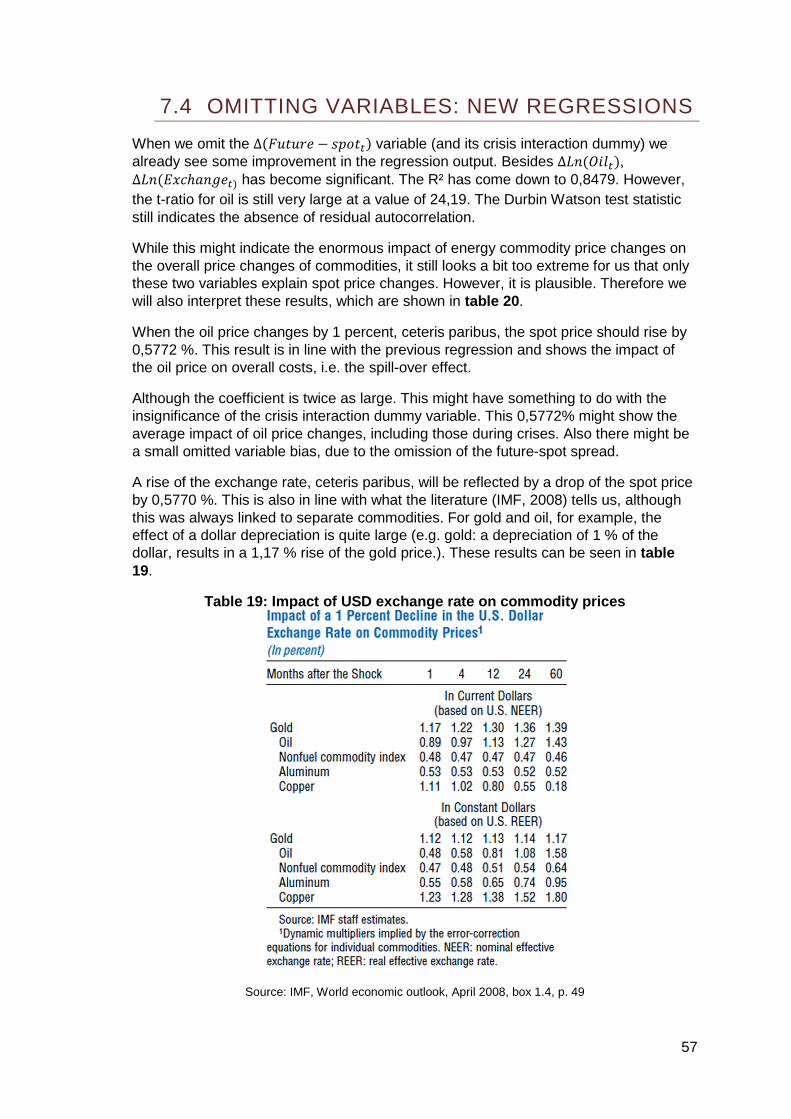
57

7.4 OMITTING VARIABLES: NEW REGRESSIONS

When we omit the ∆(�� − !"��) variable (and its crisis interaction dummy) we already see some improvement in the regression output. Besides ∆eM(H:;�), ∆eM(QZ][OM\��) has become significant. The R² has come down to 0,8479. However, the t-ratio for oil is still very large at a value of 24,19. The Durbin Watson test statistic still indicates the absence of residual autocorrelation.

While this might indicate the enormous impact of energy commodity price changes on the overall price changes of commodities, it still looks a bit too extreme for us that only these two variables explain spot price changes. However, it is plausible. Therefore we will also interpret these results, which are shown in table 20 .

When the oil price changes by 1 percent, ceteris paribus, the spot price should rise by 0,5772 %. This result is in line with the previous regression and shows the impact of the oil price on overall costs, i.e. the spill-over effect.

Although the coefficient is twice as large. This might have something to do with the insignificance of the crisis interaction dummy variable. This 0,5772% might show the average impact of oil price changes, including those during crises. Also there might be a small omitted variable bias, due to the omission of the future-spot spread.

A rise of the exchange rate, ceteris paribus, will be reflected by a drop of the spot price by 0,5770 %. This is also in line with what the literature (IMF, 2008) tells us, although this was always linked to separate commodities. For gold and oil, for example, the effect of a dollar depreciation is quite large (e.g. gold: a depreciation of 1 % of the dollar, results in a 1,17 % rise of the gold price.). These results can be seen in table 19.

Table 19: Impact of USD exchange rate on commodity prices

Source: IMF, World economic outlook, April 2008, box 1.4, p. 49

58

If we look at the response of a commodity index (non-fuel) to a 1% depreciation of the dollar, we see that the results are in line with ours. A decline of 1 % results in a rise of commodity prices of 0,48 %. The differences might be due to the fact that the IMF-research was done in 2008, during the crisis, before the full impact was visible.

The impact of the dollar depreciation is the largest for gold, oil and metals. Soft-commodities do not seem to have a high negative correlation (IMF 2008). This might have something to do with the ability of those commodities as a storage of value. Or to repeat Bhar and Hammoudeh (2010): …a flight to the safety of currency commodities such as oil in response to a weakening dollar.

Also Akram (2009) indicates that the dollar exchange rate contributes significantly to changes in commodity prices.

Although our commodity index has some soft commodities in it, these only account for about 22 % of the total index, whilst industrial metals, precious metals and energy commodities make up the other 78%. This might be an explanation why the coefficient is higher than that of a non-fuel commodity index.

Table 20: OLS-regression results: First differences without future spot spread


The results are in line with findings in the literature and are in our view realistic, but we move on and estimate the model without the ∆d%(4-+�), and its crisis interaction dummy, to see what kind of a result this regression gives us.

As was the case as well in the previous regression, the crisis interaction dummies are not significant. In this regression the only significant variable is the ∆eM(QZ]ℎOM\��) and the black swan dummy.

The R² has dropped to a record low of 0,3153 and the t-ratios of the significant variables are not as high as before. The results are presented in table 21 , below.

In this case the coefficient for the exchange rate is high and is not really in line with results of the IMF (2008). Akram (2009), however, states that the dollar exchange rate (and the real interest rate) contribute significantly to movements in commodity prices.

Variable Coefficient Variable Coefficient � -0,0011

(-0,27) ?∆d%()%231�0-,+�) 0,9786

(0,52) ∆d%(4-+�) 0,5772

(24,19) ∆d%($�%&'�) 0,5737

(0,83) ?∆d%(4-+�) 0,1559

(1,28) ?∆d%($�%&'�) -1,1044

(-0,66) ∆|x()%*+,�-�%�./) -0,0338

(-1,59) ∆d%((57,%8&�) -0,5770

(-3,74) ?P∆(�()%*+,�-�%�./ -0,0477

(-0,94) ?∆d%((567,%8&�) 0,8677

(1,16) ∆()%�&0&1�0,�&�� 0,0016

(0,36) =��0-1-1�� 0,0033

(0,29) ?∆�)%�&0&1�� -0,0126

(-0,97) =�B+,6C�D,%�� -0,0091

(-0,45) ∆d%�)%231�0-,+�� 1,0735

(1,66) R² Durbin Watson

0,8479 2,2922

59

Table 21: OLS-regression results: First differences without oil and future spot Variable Coefficient Variable Coefficient

� 0,0148 (1,83)

∆d%($�%&'�) -1,2031 (-0,83)

∆|x()%*+,�-�%�./) 0,0035 (0,08)

?∆d%($�%&'�) 3,6095 (1,03)

?P∆(�()%*+,�-�%�./ -0,0080 (-0,08)

∆d%((57,%8&�) -1,3693 (-4,31)

∆()%�&0&1�0,�&�� 0,0109 (1,16)

?∆d%�(567,%8&�� -1,5785 (-1,31)

?∆�)%�&0&1�� -0,0188 (-0,69)

=��0-1-1�� -0,0091 (-0,38)

∆d%�)%231�0-,+�� 2,4574 (1,80)

=�B+,6C�D,%�� -0,0832 (-1,99)

?∆d%�)%231�0-,+�� 3,2148 (0,87)

R² Durbin Watson

0,315250 2,128122

Source: Statistics program/ own creation

An appreciation of the dollar with 1 % might result in, ceteris paribus, a decline in commodity prices of 1, 37 %. Quite high, but still realistic (gold and oil, separately, had similar responses to the dollar exchange rate (IMF, 2008)). Though, together with the Black Swan dummy the dollar exchange rate only explains 31,52 % of price changes in commodities.

Our Black Swan dummy has become significant in this regression. It can be interpreted as follows: the presence of a Black Swan event will have a negative impact of 0,08 % on commodity prices. A very small effect and just barely significant.

7.5 A FINAL OLS REGRESSION

We will now perform a final regression, without all the crisis interaction dummies, since these don’t appear to be significant anyway38. Let’s look at the results.

We see that there are three significant variables in this model, whilst the R² is 0,29. The t-ratio’s of the significant variables are all relatively low, which excludes the possibility of a spurious regression. The Durbin Watson remains comfortably stable around 2, so there is no fear for residual autocorrelation

Table 22: OLS-regression without interaction dummie s Variable Coefficient Variable Coefficient � 0,0116

(1,50) ∆d%�(57,%8&�� -1,5207

(-5,17) ∆|x�)%*+,�-�%�./� 0,0261

(0,68) =��0-1-1�� -0,0016

(-0,11) ∆�)%�&0&1�0,�&�� 0,0109

(1,28) =�B+,6C�D,%�� -0,0751

(-2,13) ∆d%�)%231�0-,+�� 3,8453

(3,28) R² 0,2909

∆d%�$�%&'�� -0,4970

(-0,39) Durbin Watson 2,0923


38 We performed some regressions with these dummies included in various amounts, and yet they remained stubbornly insignificant.

60

∆Ln(IndustrialK), ∆Ln(ExhangeK) and our D(BlackSwanK� seem to be the best variables to explain the changes in the commodity spot price. Let us interpret their coefficients.

A rise of one percent, ceteris paribus, in industrial production , will be reflected in the spot price as a rise of 3,845 %. This might seem high, but it might indicate that the basic game of supply and demand (i.e. economic growth) remains the strongest driver for commodity price changes39.

Since we have excluded the spill-over variable ∆Ln�OilK�, we believe that there might be a small omitted variable bias so that a portion of the effect of price changes in energy commodities (like oil) has sneaked into this industrial production variable, inflating its coefficient. But then again, a growing economy requires enormous amounts of energy, so this “inflation” is acceptable from an economic point of view.

It is unfortunate that we had to exclude the proxy variable for inventories, being the ∆�Future − spott�. Although the industrial production is also related with this variable. A higher growth of industrial production (i.e. economic growth) will result in a higher demand for commodities. This will put a stress on commodity inventories, resulting in a decline of stocks, which in turn (rising demand, falling supply) causes a price increase.

There is an absence of monetary variables. Although we believe monetary variables do have an effect on commodity price changes (and vice versa), we think that part of the monetary effects are captured by the exchange rate variable.

∆Ln�ExhangeK� has a coefficient of -1,5207, which means that a rise of 1 % of the dollar exchange rate index (appreciation of the dollar, relative to the basket of foreign commodities), ceteris paribus of course, will be reflected by a drop in commodity spot prices of 1,52 %. This result is in line with the theory and previous empiric research (IMF, 2008; Akram, 2009), although our decline percentage is higher.

This might be attributable to the relatively short research period and the usage of monthly data. Also we looked at a basket of commodities (represented by the GSCI) which gives another result than research of individual commodities.

Finally we have the Black Swan dummy variable, =�B+,6C�D,%��, which has a very small effect. When a Black Swan event (ceteris paribus) occurs, there will be a drop in commodity prices of 0,075 %. This effect is very small, but yet, still significant (as it also was in the previous regression).

The strange thing with Black Swans however is there rare and unpredictable nature, making it difficult to fit them into statistical models. Although we deem it interesting to know that a Black Swan will have a significant effect on commodity prices when it occurs. Due to the widespread, global nature of commodity markets today (a form of diversification) the impact of such a rare, unpredictable event will be quite small.

Although we have some nice significant variables, which seem to support some of our theories, we must report that these only account for about 30% of price changes in commodity spot prices. The other 70% of the explanation of commodity price changes might be captured by some of our excluded variables (such as the oil price and the effect of inventories), speculation, and/or political factors.

39 It is difficult to compare this result with those in the literature, because, we used industrial production (a monthly variable), while in most cases in the literature GDP growth is used.

61

7.6 ASIDE ON LAGGED VARIABLES

Before we move on into the realm of the Vector Auto Regression, we think it is necessary to state why there are no lags present in our OLS regression output.

We did the OLS-regressions with three month lags on all the variables (basic model) and found a small amount of significant lagged variables (for oil and industrial production). However, this model had a very high R² (0,96) and we decided not to pursue this path further.

We tried a regression with three month lags as well on our final model and found that only a 2 month lag of the spot price itself was significant, together with the black swan dummy and the exchange rate. Industrial production no longer appeared to be significant. So we believe it was not an acceptable result and hence there are no lagged variables in our regressions.

7.7 CHOOSING THE RIGHT MODEL

Now that we have determined several plausible regressions, we have to choose the one that delivers the best and most reliable results. Both the first (all variables included) and the second regression (excluding the future-spot spread) provide us with a high explanatory power. So it is obvious we will opt for one of these two.

The results from both these regressions are economically plausible and in some cases downright intriguing (for example the Z∆(InterestK) crisis interaction dummy). But from an econometrical point of view we chose the version which excluded the future-spot spread, since this poses too much risk for a bias, due to its close relation to the dependent variable. It is however advisable to take the interpretation given to the results of that model also into account when dealing with commodities.

8. THE MULTIVARIATE MODEL: VAR

8.1 VECTOR AUTOREGRESSION

Can we determine which variables cause changes in t he commodity prices and vice versa, which changes are caused by a change in commodity prices?

That is the next research question on which we will try to give an answer. In order to do this we will use a VAR-model to find out which variable granger causes another. Since we have a total of 8 basic variables, we will have 8 equations. To make things not too complex, the interaction dummies are not used in this model.

We will look at the impact of each transformed variable (so with logs and first differences) on the other variables of our model. As we have stated before in chapter 6.2.3, there are six co-integration relations between these variables. Normally that would require an VECM, but that lies beyond the scope of this thesis. So, we move on to the VAR-model.

62

8.2 LAG SELECTION

Before we can estimate our VAR model, we need to determine the number of lags to add. This is done by using the information criteria. The correct lag length will be the one that yields the smallest value for the information criterion.

Since we utilize three different criteria, we will opt for the lag length for which the majority of the criteria has the smallest value. As you can see in the following table40, we will opt for a VAR model with 2 lags.

Table 23: Information criteria Lags AIC BIC HQC 1 -25,831562 -24,438976 -25,267181 2 -28,399901 -25,893245* -27,384015* 3 -28,427505 -24,806780 -26,960114 4 -28,518512* -23,783719 -26,599617 5 -28,306318 -22,457456 -25,935918 6 -28,055921 -21,092989 -25,234015


8.3 THE MODEL

8.3.1 THE EQUATION

Now that we have determined the lag length, we can move on to an introduction of our equations. As stated before we will have seven of those, each with a different variable as the dependant variable and the others as explanatory variables, each with 2 lags of itself. So we get41:

∆eM(�!"��)= 9E + �E� + �EE∆eM��!"��E� + �EG∆eM��!"��G� + #EE∆�� − !"��E�+ #EG∆�� − !"��G� + �EE∆eM�H:;��E� + �EG∆eM�H:;��G� + �EE ∆EK�LMN;O�:"M��+ �EG ∆EK�LMN;O�:"M��E� + �EE∆�LM�� O��E�+ �EG∆�LM�� O��G�+�EE∆eM�LMU� ��:O;��E�+�EG∆eM�LMU� ��:O;��G�+ �EE∆eM�W"M�X��E� + �EG∆eM�W"M�X��G�+�EE∆eM�QZℎOM\��E�+ �EG∆eM�QZℎOM\��G�+>E�

∆�� − !"��= 9G +�G� + �GE∆eM��!"��E� + �GG∆eM��!"��G�+#GE∆�� − !"��E�+ #GG∆�� − !"��G� + �GE∆eM�H:;��E� + �GG∆eM�H:;��G� + �GE ∆EK�LMN;O�:"M��+ �GG ∆EK�LMN;O�:"M��E� + �GE∆�LM�� O��E�+ �GG∆�LM�� O��G�+�GE∆eM�LMU� ��:O;��E�+�GG∆eM�LMU� ��:O;��G�+ �GE∆eM�W"M�X��E� + �GG∆eM�W"M�X��G�+�GE∆eM�QZℎOM\��E�+ �GG∆eM�QZℎOM\��G�+>G�

40 We have used the following criteria (with their abbreviations): AIC= Akaike criterion, BIC= Schwarz Bayesian criterion and HQC= Hannan-Quinn criterion 41 To save some space, we will only give the first two equations of the model, the other 6 are identically built.

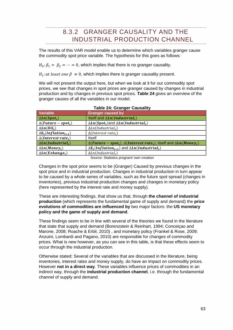
63

8.3.2 GRANGER CAUSALITY AND THE INDUSTRIAL PRODUCTION CHANNEL

The results of this VAR model enable us to determine which variables granger cause the commodity spot price variable. The hypothesis for this goes as follows:

� :#E =#G = ⋯ = 0, which implies that there is no granger causality.

�E: O�;�O �"M�# ≠ 0, which implies there is granger causality present.

We will not present the output here, but when we look at it for our commodity spot prices, we see that changes in spot prices are granger caused by changes in industrial production and by changes in previous spot prices. Table 24 gives an overview of the granger causes of all the variables in our model.

Table 24: Granger Causality Variable Granger caused by ∆d%�� Itself and ∆d%�)%231�0-,+�� ∆��3�30& − 1�� ∆d%��and ∆d%�)%231�0-,+�� ∆d%�4-+�� ∆eM�LMU� ��:O;�� ∆|x�)%*+,�-�%�./� ∆�LM�� O�� ∆�)%�&0&1�0,�&�� Itself ∆d%�)%231�0-,+�� ∆��3�30& − 1��, ∆�)%�&0&1�0,�&��, itself and ∆d%�$�%&'�� ∆d%�$�%&'�� ∆|x�)%*+,�-�%�./� and ∆d%�)%231�0-,+�� ∆d%�(57,%8&�� ∆eM�LMU� ��:O;��


Changes in the spot price seems to be (Granger) Caused by previous changes in the spot price and in industrial production. Changes in industrial production in turn appear to be caused by a whole series of variables, such as the future spot spread (changes in inventories), previous industrial production changes and changes in monetary policy (here represented by the interest rate and money supply).

These are interesting findings, that show us that, through the channel of industrial production (which represents the fundamental game of supply and demand) the price evolutions of commodities are influenced by two major factors: the US monetary policy and the game of supply and demand .

These findings seem to be in line with several of the theories we found in the literature that state that supply and demand (Borenzstein & Reinhart, 1994; Conceiçao and Marone, 2008; Roache & Erbil, 2010) , and monetary policy (Frankel & Rose, 2009; Anzuini, Lombardi and Pagano, 2010) are responsible for changes of commodity prices. What is new however, as you can see in this table, is that these effects seem to occur through the industrial production.

Otherwise stated: Several of the variables that are discussed in the literature, being inventories, interest rates and money supply, do have an impact on commodity prices. However not in a direct way . These variables influence prices of commodities in an indirect way, through the industrial production channel , i.e. through the fundamental channel of supply and demand.

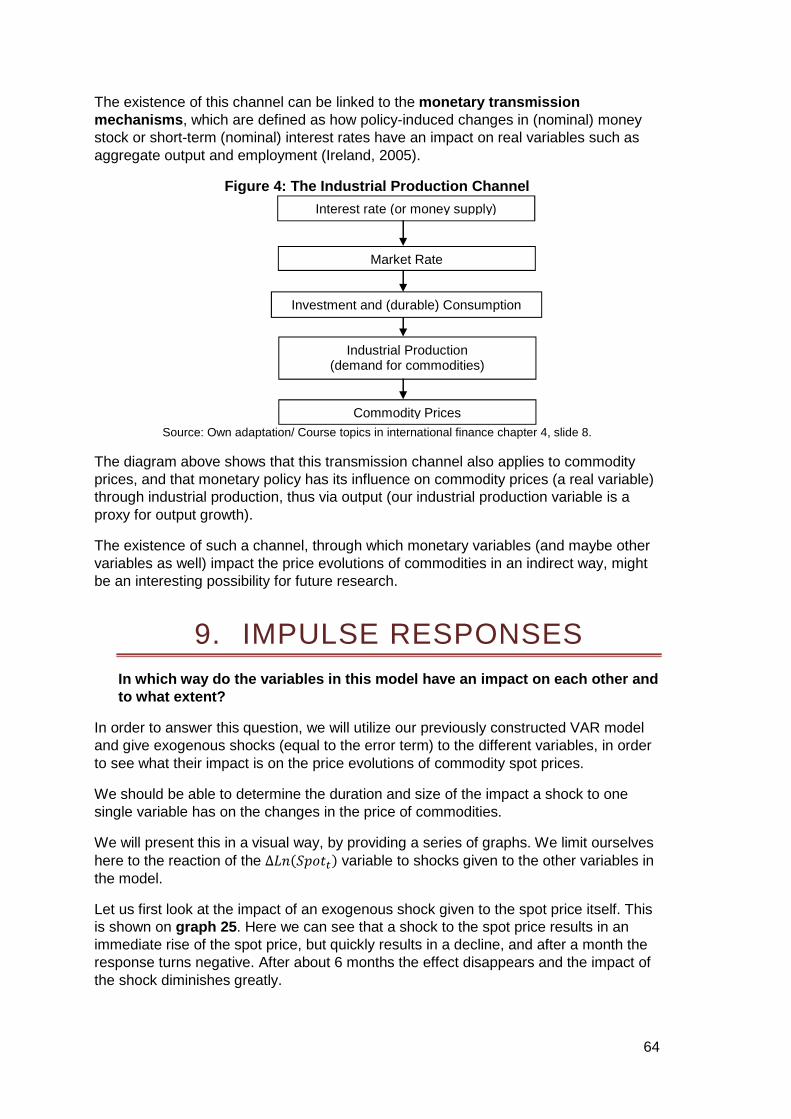
64

The existence of this channel can be linked to the monetary transmission mechanisms , which are defined as how policy-induced changes in (nominal) money stock or short-term (nominal) interest rates have an impact on real variables such as aggregate output and employment (Ireland, 2005).

Figure 4: The Industrial Production Channel

Source: Own adaptation/ Course topics in international finance chapter 4, slide 8.

The diagram above shows that this transmission channel also applies to commodity prices, and that monetary policy has its influence on commodity prices (a real variable) through industrial production, thus via output (our industrial production variable is a proxy for output growth).

The existence of such a channel, through which monetary variables (and maybe other variables as well) impact the price evolutions of commodities in an indirect way, might be an interesting possibility for future research.

9. IMPULSE RESPONSES In which way do the variables in this model have an impact on each other and to what extent?

In order to answer this question, we will utilize our previously constructed VAR model and give exogenous shocks (equal to the error term) to the different variables, in order to see what their impact is on the price evolutions of commodity spot prices.

We should be able to determine the duration and size of the impact a shock to one single variable has on the changes in the price of commodities.

We will present this in a visual way, by providing a series of graphs. We limit ourselves here to the reaction of the ∆eM(�!"��) variable to shocks given to the other variables in the model.

Let us first look at the impact of an exogenous shock given to the spot price itself. This is shown on graph 25 . Here we can see that a shock to the spot price results in an immediate rise of the spot price, but quickly results in a decline, and after a month the response turns negative. After about 6 months the effect disappears and the impact of the shock diminishes greatly.

Interest rate (or money supply)

Market Rate

Investment and (durable) Consumption

Industrial Production (demand for commodities)

Commodity Prices

65

Graph 25: Response of ∆d%(��)to a shock in ∆d%��

Source: Statistics program

Graph 26: Response of ∆d%�� to a shock in ∆��3�30& − 1��


On graph 26 we can see that a shock given to the future-spot spread, i.e. a (positive) shock to the inventories, will result in a sharp price percent price change of spot prices, as the literature says (IMF, 2008). After about three months the situation seems to recover quickly and seems to result in a positive price change after about six months. This effect declines slowly.

Graph 27 shows us the impact of a sudden change of the oil prices. This seems to result in a rapid price rise after a month (with a slower increase in the first month). However, after 2 months the trend changes and a negative price change will follow, up to about 5 months after the initial shock.

-0,02

-0,01

0

0,01

0,02

0,03

0,04

0,05

0,06

0,07

0 5 10 15 20 25

periods

response of Delta_ln_spot to a shock in Delta_ln_spot, with bootstrap confidence interval

90 percent confidence band

point estimate

-0,016

-0,014

-0,012

-0,01

-0,008

-0,006

-0,004

-0,002

0

0,002

0,004

0,006

0 5 10 15 20 25

periods

response of Delta_ln_spot to a shock in Delta_future_sp, with bootstrap confidence interval


point estimate

66

This could be explained by the fact that a too high price change of oil price might eventually result in lower demand for commodities, when commodity producers increase prices of commodities to compensate for higher oil prices.

This is almost always done with a time lag since mostly commodities are traded through term contracts. After that there seems to be a recovery, until after about 10 months the effect of the shock almost completely disappears. So, changes in oil prices seem to have only a large effect in the first six months.

Graph 27: Response of ∆d%(��) to a shock in ∆d%(4-+�)


A shock to the expected inflation, as presented on graph 28 , seems to result in a sharp decline of price changes in commodity prices. The situation stabilizes after 2-3 months. The commodity spot price changes slowly recover, to return to a normal situation after about a year.

Graph 28: Response of ∆d%(��) to a shock in ∆|x()%*+,�-�%�./)


-0,01

-0,005

0

0,005

0,01

0,015

0 5 10 15 20 25

periods

response of Delta_ln_spot to a shock in Delta_ln_oil, with bootstrap confidence interval


point estimate

-0,012

-0,01

-0,008

-0,006

-0,004

-0,002

0

0,002

0,004

0,006

0 5 10 15 20 25

periods

response of Delta_ln_spot to a shock in delta_Inflation, with bootstrap confidence interval


point estimate

67

On graph 29 we witness the impact of a shock to the real interest rate. This impact appears to be rather limited, but will result in a positive change of commodity prices, which is rather strange, since the literature speaks of a negative correlation between interest rates and commodity prices.

After about a year a negative impact emerges, but also very small. This limited impact might have something to do with the fact that in our OLS regression, the interest rate was not significant.

Graph 29: Response of ∆d%(��) to a shock in ∆()%�&0&1�0,�&��


Graph 30: Response of ∆d%�� to a shock in ∆d%�)%231�0-,+��


-0,008

-0,006

-0,004

-0,002

0

0,002

0,004

0,006

0,008

0,01

0,012

0 5 10 15 20 25

periods

response of Delta_ln_spot to a shock in Delta_Interest, with bootstrap confidence interval


point estimate

-0,006

-0,004

-0,002

0

0,002

0,004

0,006

0,008

0,01

0 5 10 15 20 25

periods

response of Delta_ln_spot to a shock in Delta_ln_Indust, with bootstrap confidence interval


point estimate

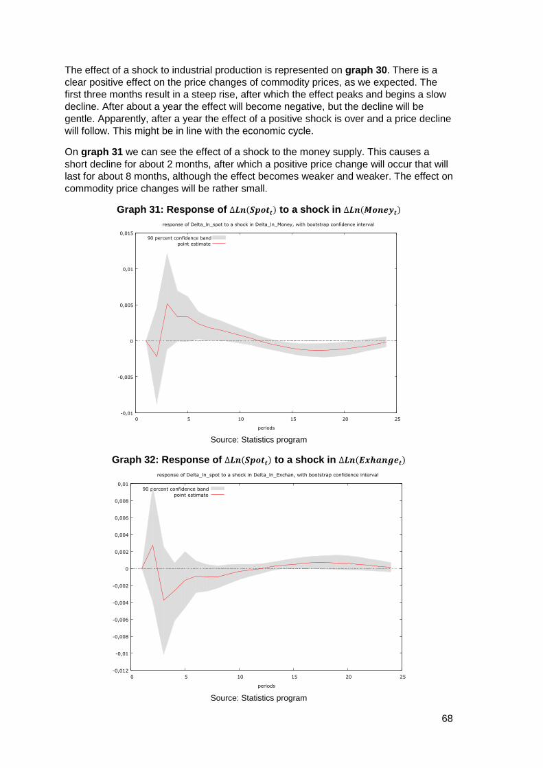
68

The effect of a shock to industrial production is represented on graph 30 . There is a clear positive effect on the price changes of commodity prices, as we expected. The first three months result in a steep rise, after which the effect peaks and begins a slow decline. After about a year the effect will become negative, but the decline will be gentle. Apparently, after a year the effect of a positive shock is over and a price decline will follow. This might be in line with the economic cycle.

On graph 31 we can see the effect of a shock to the money supply. This causes a short decline for about 2 months, after which a positive price change will occur that will last for about 8 months, although the effect becomes weaker and weaker. The effect on commodity price changes will be rather small.

Graph 31: Response of ∆d%(��) to a shock in ∆d%($�%&'�)


Graph 32: Response of ∆d%(��) to a shock in ∆d%((57,%8&�)


-0,01

-0,005

0

0,005

0,01

0,015

0 5 10 15 20 25

periods

response of Delta_ln_spot to a shock in Delta_ln_Money, with bootstrap confidence interval


point estimate

-0,012

-0,01

-0,008

-0,006

-0,004

-0,002

0

0,002

0,004

0,006

0,008

0,01

0 5 10 15 20 25

periods

response of Delta_ln_spot to a shock in Delta_ln_Exchan, with bootstrap confidence interval


point estimate

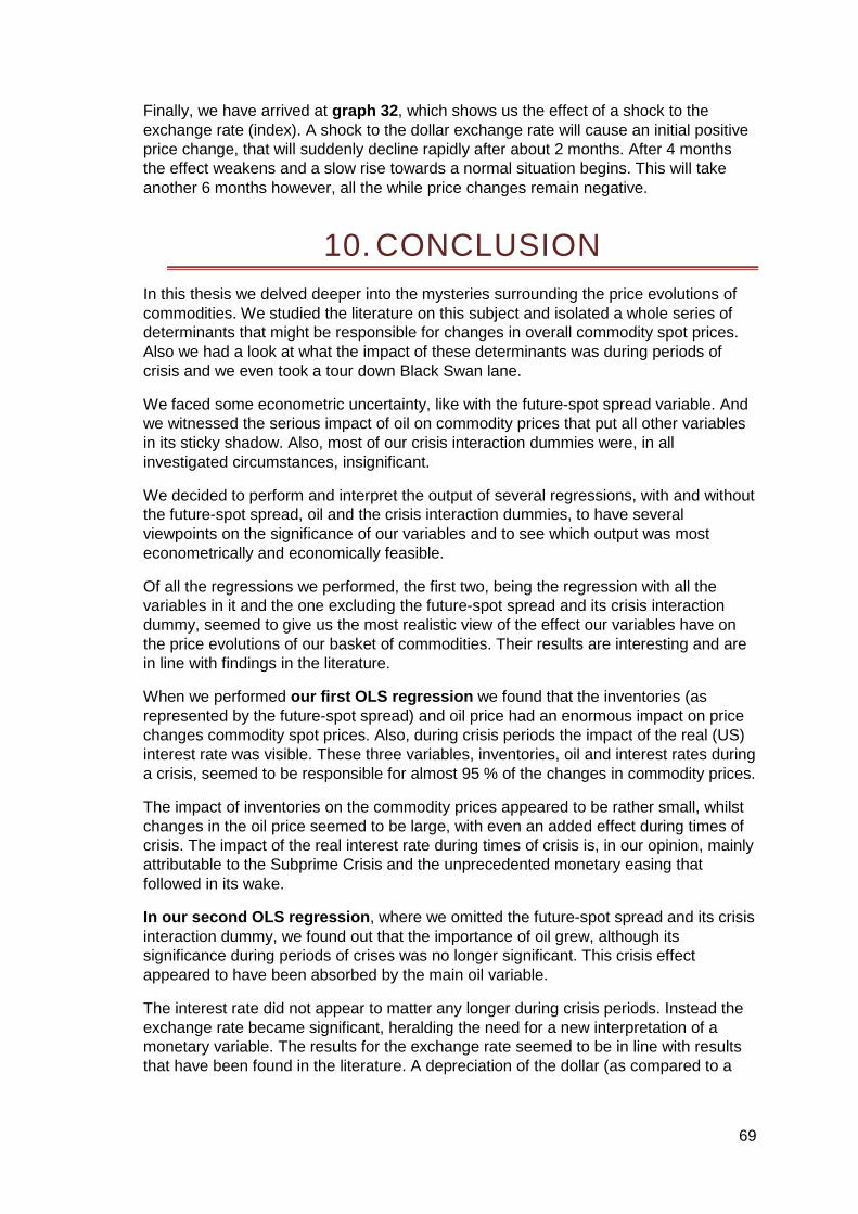
69

Finally, we have arrived at graph 32 , which shows us the effect of a shock to the exchange rate (index). A shock to the dollar exchange rate will cause an initial positive price change, that will suddenly decline rapidly after about 2 months. After 4 months the effect weakens and a slow rise towards a normal situation begins. This will take another 6 months however, all the while price changes remain negative.

10. CONCLUSION In this thesis we delved deeper into the mysteries surrounding the price evolutions of commodities. We studied the literature on this subject and isolated a whole series of determinants that might be responsible for changes in overall commodity spot prices. Also we had a look at what the impact of these determinants was during periods of crisis and we even took a tour down Black Swan lane.

We faced some econometric uncertainty, like with the future-spot spread variable. And we witnessed the serious impact of oil on commodity prices that put all other variables in its sticky shadow. Also, most of our crisis interaction dummies were, in all investigated circumstances, insignificant.

We decided to perform and interpret the output of several regressions, with and without the future-spot spread, oil and the crisis interaction dummies, to have several viewpoints on the significance of our variables and to see which output was most econometrically and economically feasible.

Of all the regressions we performed, the first two, being the regression with all the variables in it and the one excluding the future-spot spread and its crisis interaction dummy, seemed to give us the most realistic view of the effect our variables have on the price evolutions of our basket of commodities. Their results are interesting and are in line with findings in the literature.

When we performed our first OLS regression we found that the inventories (as represented by the future-spot spread) and oil price had an enormous impact on price changes commodity spot prices. Also, during crisis periods the impact of the real (US) interest rate was visible. These three variables, inventories, oil and interest rates during a crisis, seemed to be responsible for almost 95 % of the changes in commodity prices.

The impact of inventories on the commodity prices appeared to be rather small, whilst changes in the oil price seemed to be large, with even an added effect during times of crisis. The impact of the real interest rate during times of crisis is, in our opinion, mainly attributable to the Subprime Crisis and the unprecedented monetary easing that followed in its wake.

In our second OLS regression , where we omitted the future-spot spread and its crisis interaction dummy, we found out that the importance of oil grew, although its significance during periods of crises was no longer significant. This crisis effect appeared to have been absorbed by the main oil variable.

The interest rate did not appear to matter any longer during crisis periods. Instead the exchange rate became significant, heralding the need for a new interpretation of a monetary variable. The results for the exchange rate seemed to be in line with results that have been found in the literature. A depreciation of the dollar (as compared to a

70

basket of foreign currencies) results in a rise of commodity prices. This version of our model was able to explain the price evolutions of commodities for about 85 %.

If a decision should be made, we would opt for the regression that excludes the future-spot variable , since this might give biased results due to its relation with the dependant variable.

Nonetheless, the effect oil has on commodity prices cannot be neglected (in both our “winning” models) and should certainly be taken into account when devising policy , whether it is monetary (commodities have a large impact on inflation) or economic (if commodity prices are too high, economic growth will be slowed, eventually resulting in a standstill and recession).

Also investors in commodities should keep a keen eye on the evolutions of the oil price and keep in mind that there is a large spill-over effect onto other commodity classes, especially during crisis periods.

Of all our monetary variables, the dollar exchange rate seems to have the largest impact on commodity price evolutions. This variable too should be taken into account when investing in commodities, or when central banks or governments think about policy.

Although the almighty dollar today does not have the glamour of previous decades as the worlds reserve currency anymore, it is still a force to be reckoned with. When investing in commodities, we would advise to watch the steps of the FED carefully , even more so during crisis periods and their aftermath, especially since at such times there is also the possibility that the interest rate will have an impact on commodity prices.

With the help of a multivariate VAR model we were able to determine Granger Causality for our variables. This showed something interesting: Apparently only industrial production, and previous commodity (spot) price changes seem to have a direct influence on commodity price evolutions.

Indirectly , through the channel of industrial production, evolutions of commodity prices seem to be caused as well by monetary policy (interest rates and money supply) and the fundamental game of supply and demand (inventories and previous industrial production). Otherwise stated: we were able to determine a channel through which monetary policy and inventory levels influence comm odity prices in an indirect way. These findings appear to be in line with some of the current theories on monetary transmission channels.

We also had a look at the behavior of the commodity spot prices when we gave exogenous shocks to the independent variables in our model. The results showed us (in a graphical way) that in most cases the effect of such a shock on commodity prices ebbs away after about a year, with the strongest effects in the first six months after the shock. The only exemptions to this were the impact of a shock given to the spot price itself and to industrial production.

An exogenous shock given to the spot price seems to cause an immediate rise of commodity prices, followed by a quick steep dive, into a small negative price change. After 6 months the effect disappears, so compared to the other variables the effect is short-lived.

71

A shock given to the industrial production variable seems to have a long lived effect (at least 2 years after the shock). Also, the response of commodity prices to this shock in industrial production is more smoothly than a response to shocks in the other variables.

To put our findings in the light of current economic events , being the rise and sub-sequent fall of commodity prices (like oil and silver), we see that the largest impact seems to originate from the determinants we found to be significant in this thesis.

The oil price, boosted by the political unrest in the Middle East seems to have pushed up commodity prices in the previous months. The Quantative Easing (QE2) program of the US also added to the recent boom of commodity prices through, as we discovered, the industrial production channel.

We saw however, during May, that when an end comes to the monetary easing (no QE3), the prices of commodities fall. This includes the oil price, which in turn caused commodity prices to fall further.

The drop of the oil price was also attributable to some easing of the tension in the middle east and the dead of Osama Bin Laden. The spill-over effect also works in a reversed way. When the price of oil drops, the prices of commodities affected by it will fall as well.

Whether this puts an end to the current commodity boom is not clear. The situation in the Middle East remains volatile and so is the oil price. Furthermore it is not yet sure that the Fed will increase its interest rates anytime soon. It will not go for another round of QE however, and that already had its impact on the markets.

What the dollar exchange rate will do will be a more profound factor on what will occur on the commodity markets in the forthcoming months. Will it regain its strength (due to the European Sovereign Debt crisis) or will it decline further, giving room to a new rise of commodity prices?

And let us off course not forget the fundamentals, the game of supply and demand (mostly from China). If demand for commodities drops and the economy plunges into a new recession, commodity prices will drop, because as we have seen, the changes of commodity prices are Granger Caused by industrial production.

And what is truly the impact of speculation? For sure it is influenced by the monetary policy and the search for yield of investors, but to what extent do speculative positions have their impact on the prices of commodities?

Only time will tell…

72

11. OVERVIEW OF TABLES, GRAPHS AND FIGURES

11.1 GRAPHS

Graph 1: The term structure of commodity futures ............................................... 13 Graph 2: S&P GSCI Commodity Spot - Price Index ............................................... 26 Graph 3: Inverse relationship inventories and price s ............................................ 27 Graph 4: Non-linearity of convenience yield and inv entories ............................... 29 Graph 5: Inverse relationship Future spot spread an d Spot prices ...................... 30 Graph 6: Relationship inventory levels and price vo latility ................................... 30 Graph 7: US Money Supply (M2) ............................................................................. 31 Graph 8: Expected annual Inflation ......................................................................... 33 Graph 9: Real interest rate ....................................................................................... 34 Graph 10: Industrial Production .............................................................................. 35 Graph 11: S&P GSCI Crude Oil Spot price index ................................................... 36 Graph 12: The dollar exchange rate index .............................................................. 37 Graph 13: Non-stationary series d%(��). ........................................................... 41 Graph 14: Stationary series ∆d%(��) ................................................................. 41 Graph 15: XY-plot ∆d%(��).vs ∆(�3�30& − 1��) ............................................. 45 Graph 16: XY-plot d%(��). vs �3�30& − 1��.................................................... 46 Graph 17: XY-plot ∆st(uvwxx). vs ∆st(yz{x) ............................................................ 46 Graph 18: XY-plot ∆st(uvwxx). vs ∆|x(}t~{�xzwtx + /) ............................................ 47 Graph 19: XY-plot st(uvwxx) vs |x(}t~{�xzwtx + /).................................................. 48 Graph 20: XY-plot ∆st(uvwxx) vs ∆(}tx��xx) ........................................................ 48 Graph 21: XY-Plot st(uvwxx) vs }tx��xx ............................................................... 49 Graph 22: XY-plot ∆st(uvwxx) vs ∆d%()%231�0-,+�) ............................................... 50 Graph 23: XY-plot ∆st(uvwxx) vs ∆st(�wt��x) ....................................................... 50 Graph 24: XY-plot ∆d%(��) vs ∆d%((567,%8&�) ................................................ 51 Graph 25: Response of ∆d%�� to a shock in ∆d%�� ..................................... 65 Graph 26: Response of ∆d%�� to a shock in ∆�3�30& − 1�� ......................... 65 Graph 27: Response of ∆d%�� to a shock in ∆d%4-+� ....................................... 66 Graph 28: Response of ∆d%�� to a shock in ∆|x)%*+,�-�%� + / ...................... 66 Graph 29: Response of ∆d%�� to a shock in ∆)%�&0&1� 0,�&� .......................... 67 Graph 30: Response of ∆d%�� to a shock in ∆d%)%231�0-,+� .......................... 67 Graph 31: Response of ∆d%�� to a shock in ∆d%$�%&'� ................................. 68 Graph 32: Response of ∆d%�� to a shock in ∆d%(57,%8&� ............................. 68

73

11.2 TABLES

Table 1: Differences between forwards and futures ...............................................12 Table 2: Overview of GSCI commodities .................................................................16 Table 3: Crisis periods ..............................................................................................21 Table 4:Cash Cost of Production of Basic Metals (US dollars per ton) .................23 Table 5: Timing of the Survey of Professional Forec asters ...................................32 Table 6: Transformation to monthly data ................................................................32 Table 7: Summary of variables .................................................................................38 Table 8: Overview of logaritms .................................................................................39 Table 9: Augmented Dickey-Fuller test results .......................................................40 Table 10: Augmented Dickey-Fuller test results .....................................................42 Table 11: Johansen test for co-integration ..............................................................42 Table 12: Summary Statistics 1 ................................................................................44 Table 13: Summary Statistics 2 ................................................................................45 Table 14: correlation matrix : spot, expected infla tion and real interest rate .......49 Table 15: Correlation matrix: Main variables ...........................................................51 Table 16: Ols-regression results: Levels .................................................................52 Table 17: OLS-Regression results: First differences with oil and future-spot ......54 Table 18: OLS-regression results: First differences for period 1995-2007 ............56 Table 19: Impact of USD exchange rate on commodity prices ..............................57 Table 20: OLS-regression results: First differences without future spot spread .58 Table 21: OLS-regression results: First differences without oil and future spot ..59 Table 22: OLS-regression without interaction dummie s ........................................59 Table 23: Information criteria ...................................................................................62 Table 24: Granger Causality .....................................................................................63

11.3 FIGURES

Figure 1: Breakdown of commodity futures returns ...............................................15 Figure 2: S&P GSCI weights .....................................................................................16 Figure 3: Percentage change in real industrial comm odity prices 1862-1999 ......17 Figure 4: The Industrial Production Channel …………………………………………..64

74

12. BIBLIOGRAPHY

WEBSITES

http://www.economist.com/research/economics/searchActionTerms.cfm?query=commodity – 26/02/2011

http://www.oup.com/us/companion.websites/0195114701/?view=usa – 26/02/2011

http://www.economist.com/research/economics/searchActionTerms.cfm?query=spot+market – 27/02/2011

http://www.gmo.com/America/ - 28/02/2011

http://www2.goldmansachs.com/services/securities/products/sp-gsci-commodity-index/approach.html - 01/03/2011

http://www.standardandpoors.com/indices/sp-gsci/en/us/?indexId=spgscirg--usd----sp------ - 01/03/2011, S&P commodity indices: factsheet,

http://www.crbtrader.com/crbindex/spot_current.asp - 01/03/2011

http://www.crbtrader.com/crbindex/spot_background.asp - 01/03/2011

http://thomsonreuters.com/products_services/financial/thomson_reuters_indices/indices/commodity_indices/#tab1 – 01/03/2011

http://www.oecd.org/document/25/0,3746,en_36734052_36761800_36999961_1_1_1_1,00.html – 02/03/2011

http://www.nber.org/cycles/cyclesmain.html - 01/03/2011

http://www.philadelphiafed.org/research-and-data/real-time-center/survey-of-professional-forecasters/ - 02/03/2011, the file with the data can be found on http://www.philadelphiafed.org/research-and-data/real-time-center/survey-of-professional-forecasters/historical-data/mean-forecasts.cfm , Mean forecast data for levels.

http://www.federalreserve.gov/releases/h10/Summary/ -12/12/2010

NON-SCIENTIFIC SOURCES

Bernanke B. June 9, 2008. Speech: outstanding issues in the analysis of inflation. Federal reserve bank of Boston’s 53rd annual economic conference.

De Leus, K (KBC Securities). 26/11/2010. Investeren in grondstoffen (2): negatief rendement voorbije jaren bij doorrollen futures ondermijnt risicopremie, Beurs bij ’t ontbijt (BBTO).

De Standaard. 24/05/2005. Grondstoffen als langetermijnbelegging: Olie en metalen hebben een plaats in uw portefeuille. Bijlage DS fondsen -– p.5

Krugman, P., 12 May 2008. “The oil nonbubble”. The new York Times

75

SCIENTIFIC SOURCES

BOOKS

Dubofsky, D.A.,& Miller T.W. 2002, Derivatives: Valuation and Risk Management. Chapter 1.

IMF. April 2008. World economic outlook, p. 48-57

Koop, G. 2006. Analysis of financial data, p.102-171

Montier, J. 2007. Behavioural Investing, chapter 49.

Montier, J. May 2010. I want to break free or, Strategic Asset Allocation ≠ Static Asset Allocation. GMO, p.10-11

Taleb, N. N. 2010. The Black Swan, second edition, 2010, p xxii-xxiii

Van Overtveldt, J. 2009. Maandag geen economie meer?, chapter 2, p.59-92

PAPERS

Anzuini, A., Lombardi, M.J., & Pagano, P. 2010. The impact of monetary policy shocks on commodity prices. ECB working paper series nr.1232.

Baelen, L., & Inghelbrecht, K. 2006. Time-Varying Integration, Interdependence and Contagion, p.27

Borenzstein, E., & Reinhart, C.M. 1994. The Macroeconomic Determinants of Commodity Prices. IMF staff paper vol.41 (2)

Barsky, R. & Kilian, L. 2004. Oil and the Macro economy since the 1970s. NBER Working paper No. 10855. JEL No. E31, E32.

Carpantier, J. 2010. Commodities Inventory Effect. Ecore discussion paper 2010/78, p. 4-5

Cashin, P., & McDermott, C.J. 2001. The long-run behavior of commodity prices: small trends and big variability. IMF working paper WP/01/68.

Centrale Raad voor het Bedrijfsleven. 25/03/2009. Inflatie in internationaal perspectief. p 11-14.

Chen, Y., Rogoff, K., & Rossi, B. 2009. Can exchange rates forecast commodity prices?

Coenraets, J. 2006. Commodity Hedging & -Investment; p. 9-32

Conceiçao, P., & Marone , H. 2008. Characterizing the 21st century first commodity boom: Drivers and impact. UNDP working paper, p. 25-30

De Smedt, T. 2010. Een analyse van de grondstoffenmarkten, p. 30-32.

ECB Eurosystem. September 2009. OTC derivatives and post-trading infra structures.

Frankel, J.A. 2006.The effect of monetary policy on real commodity prices, p. 21

76

Frankel, J.A., & Rose, A.K. 2009. Determinants of agricultural and mineral commodity prices, p.3-24

Gorton, G.B., & Rouwenhorst K.G. 2005. Facts and fantasies about commodity futures.

Gorton, G.B., Hayashi, F., & Rouwenhorst K.G. 2008. The fundamentals of commodity futures returns.

Ireland, P.N. 2005. The Monetary Transmission Mechanism, p.1

Kilian, L. 2007. A comparison of the effects of exogenous oil supply shocks on output and inflation in the G7 countries.

Österholm, P. 2003. The Taylor Rule: A Spurious Regression?

Roache, S., & Erbil, N. 2010. How commodity price curves and inventories react to a short-run scarcity shock. IMF working paper, WP/10/222.

Rogoff, K. 2006. Oil and the Global Economy.

UNCTAD. 2009. Trade and development report, chapter 2: The financialization of commodity markets, p 54-57

SCIENTIFIC JOURNALS

Akram, Q.F. 2009. Commodity prices, interest rates and the dollar, Energy Economics 31, p. 838-851.

Baffes, J. 2007. Oil spills on other commodities, Resources policy 32, p 126-134.

Bhar, R. & Hammoudeh, S., Commodities and financial variables: Analyzing relationships in a changing regime environment, International Review of Economics and Finance (2010), doi: 10.1016/j.iref.2010.07.011.

Browne, F., & Cronin, D. 2010. Commodity prices, money and inflation, Journal of economics and business 62, p. 331-345.

Cashin, P., Mc Dermott, C.J., & Scott, A. 2002. Booms and slumps in world commodity prices, Journal of development economics 69, p. 277-296,

Radetzki, M. 2006. The anatomy of three commodity booms, Marian, Resources policy 31, p. 56-64.

Price evolutions on the commodity markets.

Documents

Transcript of Price evolutions on the commodity markets.