Price Elasticities for Energy Use in Buildings of the ... · Price Elasticities for Energy Use in...

Price Elasticities for Energy Use in Buildings of the United States

October 2014

Independent Statistics & Analysis

www.eia.gov

U.S. Department of Energy

Washington, DC 20585

U.S. Energy Information Administration | Price Elasticities for Energy Use in Buildings of the United States i

This report was prepared by the U.S. Energy Information Administration (EIA), the statistical and analytical agency within the U.S. Department of Energy. By law, EIA’s data, analyses, and forecasts are independent of approval by any other officer or employee of the United States Government. The views in this report therefore should not be construed as representing those of the Department of Energy or other federal agencies.

October 2014

U.S. Energy Information Administration | Price Elasticities for Energy Use in Buildings of the United States ii

Table of Contents

Introduction ............................................................................................................................................. 1

Energy demand: Permanent and temporary all fuel prices doubled cases ............................................. 2

Own-price and cross-price elasticities ..................................................................................................... 5

Energy demand: Natural gas consumption in the elasticity cases .......................................................... 6

Energy demand: Electricity consumption and electric end uses in the Electricity Price Doubled case 10

Costs in elasticity cases .......................................................................................................................... 17

Conclusion.............................................................................................................................................. 20

Appendix ................................................................................................................................................ 21

October 2014

U.S. Energy Information Administration | Price Elasticities for Energy Use in Buildings of the United States iii

Tables Table 1. Summary of own-price elasticities in AEO2014 Residential and Commercial Demand Modules ........................................................................................................................................................ 5 Table 2. Summary of cross-price elasticities in AEO2014 Residential and Commercial Demand Modules (Long Run, Year 25) ......................................................................................................... 6 Table 3. Changes in residential heating equipment stock, 2040 ................................................................ 13 Table 4. Summary of own-price elasticities in AEO2014 Residential and Commercial Demand Modules (using simulations where fuel price is cut in half between 2015 and 2040)................. 21 Table 5. Summary of cross-price elasticities in AEO2014 Residential and Commercial Demand Modules, Year 25 (using simulations where fuel price is cut in half between 2015 and 2040) ........................................................................................................................................... 21

October 2014

U.S. Energy Information Administration | Price Elasticities for Energy Use in Buildings of the United States iv

Figures Figure 1. Delivered energy in the commercial sector ................................................................................... 3 Figure 2. Delivered energy in the residential sector ..................................................................................... 4 Figure 3. Natural gas consumption in the residential sector across price cases .......................................... 7 Figure 4. Natural gas consumption in the commercial sector across price cases ........................................ 8 Figure 5. CHP capacity in price cases ............................................................................................................ 9 Figure 6. Natural gas consumption for space heating in the commercial sector ....................................... 10 Figure 7. Electricity consumption in the commercial sector across price cases ......................................... 11 Figure 8. Electricity consumption in the residential sector across price cases ........................................... 12 Figure 9. Percent improvement in efficiency of residential cooling equipment in the Electricity Price Doubled case over the Reference case .............................................................................................. 14 Figure 10. Percent improvement in efficiency of commercial cooling equipment in the Electricity Price Doubled case over the Reference case .............................................................................................. 15 Figure 11. Lighting service demand for the commercial sector, Reference case vs. Electricity Price Doubled case ...................................................................................................................................... 16 Figure 12. Ventilation service demand for the commercial sector, Reference case vs. Electricity Price Doubled case ...................................................................................................................................... 17 Figure 13. Total fuel expenditures for energy customers in price cases .................................................... 18

October 2014

U.S. Energy Information Administration | Price Elasticities for Energy Use in Buildings of the United States 1

Introduction Energy demand tends to be responsive to changes in energy prices, a concept in economics known as price elasticity. Generally, an increase in a fuel price causes users to use less of that fuel or switch to a different fuel. The extent to which each of these changes takes place is of high importance to stakeholders in the energy sector and especially in energy planning. The purpose of this analysis is to determine fuel-price elasticities in stationary structures, particularly in the residential and commercial sectors.

The Residential Demand Module (RDM) and Commercial Demand Module (CDM) are two modules within the National Energy Modeling System (NEMS) at the U.S. Energy Information Administration (EIA). The RDM and CDM are used by EIA to model energy use in the residential and commercial sectors. They are updated and maintained separately, but also have shared characteristics and functions due to similarities between them. Due to these similarities, EIA sometimes uses the term buildings sector or buildings sectors to refer to the residential and commercial demand sectors in tandem.

The following analysis starts with the buildings modules as they exist in the Reference case of the 2014 Annual Energy Outlook (AEO2014) and then simulates different price paths for fuels out to 2040. Only the buildings modules are used in these simulations; integrated effects with the rest of NEMS are not included.1 The resulting changes in energy demand are analyzed and used to calculate fuel-price elasticities.

The modules allow for both short-run and long-run responses by consumers in the buildings sectors.2 Short-run responses are more behavioral and temporary in nature. An example of a short-run response would be a building occupant turning down their thermostat during cold weather in response to high energy bills. This action reduces energy demand for heating. A long-run response would be installing a more-efficient heating system or upgrading windows and insulation in a building. These long-run responses involve more durable changes and usually take place over a longer time horizon as technology and market development change building shells and the appliances and equipment that go into buildings.

1 NEMS is an integrated, modular system where fuel prices and energy demand interact until an equilibrium is met for the entire system for each model year. In the buildings modules of NEMS, energy demand equilibrates to fuel prices from other modules. Although year-to-year changes in fuel price have their largest effect on energy demand in the year in which they occur, the full effect of fuel price change is also spread over the following two years in order to prevent unrealistic demand responses to price spikes of one year or other short-term duration. This is why Tables 1 and 2 present elasticity results for Years 1-3, where Year 1 in the model is when the simulated price change from Reference case was programmed to take place and Year 2 and Year 3 are the two following years (Year 1 corresponds to 2015 in the model). 2 In economics, the short run is generally defined as a period over which capital stock remains fixed. But, because the typical service lifetime of installed capital can vary among economic sectors, energy end uses, and equipment types, there is no single definition that differentiates between short and long run.

October 2014


This analysis presents the following simulations:3

• Reference case: fuel prices remain untouched; results from buildings modules are as they appear in AEO2014, without additional effects from other modules of NEMS.

• Electricity Price Doubled case: just the electricity price doubled between 2015 and 2040. • Natural Gas Price Doubled case: just the natural gas price doubled between 2015 and 2040. • Distillate Price Doubled case: just the distillate fuel oil price doubled between 2015 and 2040. • Permanent All Fuel Prices Doubled case: prices for all three fuels (electricity, natural gas, and

distillate fuel oil) doubled between 2015 and 2040. • Temporary All Fuel Prices Doubled case: prices for all three fuels (electricity, natural gas, and

distillate fuel oil) doubled, but for a temporary period between 2020 and 2025.

Energy demand: Permanent and temporary all fuel prices doubled cases Figure 1 shows the results of the Permanent All Fuel Prices Doubled case and the Temporary All Fuel Prices Doubled case for the commercial sector. When prices are permanently doubled, energy demand drops below the Reference case in 2015, reaching 14.7% (1.3 quadrillion Btu) below Reference case in 2017. The gap between the Reference case and the Permanent Prices Doubled case appears to stay constant, but actually widens slightly in absolute terms to 2040—reaching 14.4% (1.5 quadrillion Btu) below the Reference case at that point—as equipment and building stock continue to be replaced with more-efficient options. The preference for more-efficient options occurs in response to the higher fuel prices.

In contrast, the Temporary Prices Doubled case projects a drop in energy demand to a similar level between 2020 and 2025 and then shifts back towards the Reference case a few years later. By 2028, the gap between the Temporary Prices Doubled case and the Reference case is only about 1.5% (0.1 quadrillion Btu). This gap below the Reference case continues to narrow through the rest of the projection, but does not actually meet the Reference case by 2040. This continued difference is the result of some long-run effects that became built-in during the price shock years. The upgrades in equipment and building shells purchased during the temporary price shock continue to provide some energy savings even after prices return to Reference case levels in 2025.

3 Elasticity calculations are done by taking energy demand projections in the three cases where a single fuel price is doubled and comparing that to the projected energy demand in the Reference case.

October 2014


Figure 1. Delivered energy in the commercial sector quadrillion Btu

Figure 2 shows the energy demand projections in the residential sector for the two cases. The results are similar to those in the commercial sector, but with a few additional interesting features. Both sectors see an initial drop when price changes take effect, but instead of a near-constant gap between energy demand in the Reference case and the Permanent Prices Doubled case as in the commercial sector, residential demand shows a widening gap after the initial drop.4 Energy demand in the residential sector drops by 11.0% (1.2 quadrillion Btu) below the Reference case by 2017 and then continues falling to 16.4% (1.8 quadrillion Btu) below the Reference case in 2040. Additionally, compared to the commercial sector, energy demand in the Temporary Prices Doubled case does not get as close to the Permanent Prices Doubled simulation between 2022 and 2025 and keeps a larger gap with the Reference case through 2040. Higher shares of equipment with shorter lifetimes (such as minor end uses and electric devices) and faster turnover of floorspace in the commercial sector compared to the residential sector help to explain why these gaps get narrower in the commercial sector. 5

4 In the commercial sector, the gap in energy demand between Reference case and the Permanent Prices Doubled case does increase in absolute terms from 2017 to 2040, but slowly from 1.3 quadrillion Btu to 1.5 quadrillion Btu. 5 In the Temporary Prices Doubled case, consumer purchases look like the Permanent Prices Doubled case in the years affected by fuel price spikes, but then look like the Reference case in the years not affected by fuel price spikes. Faster turnover in the commercial sector means that more consumer purchases take place in the commercial sector than in the residential sector. Thus, in the Temporary Prices Doubled case there are more consumer purchases in the commercial sector that look like each of

7

8

9

10

11

12

2010 2015 2020 2025 2030 2035 2040

Reference case Temporary All Doubled Permanent All Doubled

October 2014


Figure 2. Delivered energy in the residential sector

the other two cases, and that is one reason energy demand in the Temporary Prices Doubled case gets closer to the other two cases in the commercial sector than in the residential sector.

9.0

9.5

10.0

10.5

11.0

11.5

12.0

2010 2015 2020 2025 2030 2035 2040

Reference case Temporary All Doubled Permanent All Doubled

October 2014


Own-price and cross-price elasticities The two types of fuel price elasticity that are calculated in this analysis are own-price and cross-price elasticities. Own-price elasticity refers to changes in consumption of a particular fuel when the price for that fuel changes (for example, electricity use changes when electricity price changes), and cross-price elasticity refers to changes in consumption of a particular fuel when the price of a different fuel changes (for example, the change in electricity use when the price of natural gas changes). Own-price elasticities are usually negative—denoting that fuel consumption goes down as the price of that fuel goes up—and cross-price elasticities are usually positive—consumption of a fuel goes up when the price of a competing fuel goes up. The elasticities in Tables 1 and 2 show the percentage change in fuel use for a 1% increase in fuel price (in Table 1, for example, a 1.0% increase in electricity price results in a 0.12% decrease in electricity use in Year 1). The elasticities are calculated by taking energy demand in the Electricity Price Doubled Case, the Natural Gas Price Doubled case, and the Distillate Fuel Price Doubled case, and comparing those results to the Reference case.6

Table 1. Summary of own-price elasticities in AEO2014 Residential and Commercial Demand Modules

Short Run Long Run

Year 1 Year 2 Year 3 Year 25

Residential

Electricity -0.12 -0.21 -0.24 -0.40

Natural Gas -0.08 -0.14 -0.17 -0.28

Distillate Fuel -0.08 -0.14 -0.17 -0.20

Commercial

Electricity -0.12 -0.20 -0.25 -0.82

Natural Gas -0.14 -0.24 -0.29 -0.45

Distillate Fuel -0.14 -0.24 -0.29 -0.42

6 As mentioned before, elasticity calculations are done using simulations where a single fuel price is doubled. However, calculated elasticites would be different if different price paths were used. For example, the attached Appendix shows elasticities that result if individual fuel prices are cut in half instead of doubled. The differences between the two sets of elasticites are caused by existing market conditions and consumer preferences in the buildings sectors. (For example, the higher natural gas elasticity relative to electricity prices in Table 2 compared to Table 5 in the Appendix is due to the economic attractiveness of natural gas-driven combined heat and power when the electricity price doubles—see Figure 5 below. This does not occur when electricity prices are cut in half and thus results in a lower elasticity.)

October 2014


Table 2. Summary of cross-price elasticities in AEO2014 Residential and Commercial Demand Modules (Long Run, Year 25)

Change in fuel price:

Electricity Natural Gas Distillate

Cha

nge

in fu

el u

se:

Residential

Electricity -- 0.01 0.00

Natural Gas 0.13 -- 0.00

Distillate Fuel 0.02 0.01 --

Commercial



Distillate Fuel -0.03 0.06 --

Table 1 shows that the commercial sector contains larger own-price elasticities than the residential sector in most cases, and that the largest energy demand changes in the long run come in response to electricity prices. Short-run elasticities range from -0.08 to -0.14 in Year 1 and from -0.17 to -0.29 in Year 3. Long-run elasticities at Year 25 ranged from -0.20 to -0.82. Table 2 shows that the commercial sector also contains larger cross-price elasticities.

Energy demand: Natural gas consumption in the elasticity cases Figures 3 and 4 show natural gas demand in the residential and commercial sectors for the cases when a single fuel price is doubled and the Permanent All Fuel Prices Doubled case. In the residential sector, the higher natural gas demand in the simulation with the doubled electricity price reflects the positive long-run cross-price elasticity that natural gas has with electricity prices in Table 2 (+0.13). The larger drop in the simulation where the natural gas price is doubled correlates with the larger negative long-run own-price elasticity of natural gas in Table 1 (-0.28). The long-run cross-price elasticity of 0 with respect to distillate fuel prices explains why the demand line in Figure 3 for the Distillate Price Doubled case basically does not change from the Reference case. Natural gas demand decreases when all fuel prices double, but it does not drop as far as when the natural gas price doubles by itself. This is because the doubling of the other prices keeps natural gas competitive, meaning fewer consumers in the buildings sectors switch to other fuels than if only the natural gas price were doubled. However, as Figure 2 shows, total delivered energy in the sector drops by 1.8 quadrillion Btu in 2040 when all fuel prices are doubled. Thus, when all fuel prices are doubled, the reduction in natural gas demand is caused more by increasing efficiency and forgoing energy services than by fuel switching.

October 2014


Figure 3. Natural gas consumption in the residential sector across price cases quadrillion Btu

Similar dynamics are illustrated in the commercial sector in Figure 4, except that the long-run own-price elasticity of natural gas is -0.45, and the long-run cross-price elasticity with respect to the electricity price is 1.24. These larger elasticities are consistent with the wider range of natural gas demand between the simulations in 2040 in the commercial sector, relative to the residential sector. Additionally, when all prices are doubled the initial decline in natural gas demand is similar to the residential sector. But, while this demand maintains a significant gap with the Reference case in the residential sector (see Figure 3), it essentially returns to Reference case levels in the commercial sector by 2040 (see Figure 4).

3.0

3.5

4.0

4.5

5.0

5.5

2010 2015 2020 2025 2030 2035 2040

Reference case Permanent All DoubledNatural Gas Doubled Electricity DoubledDistillate Doubled

October 2014


Figure 4. Natural gas consumption in the commercial sector across price cases quadrillion Btu

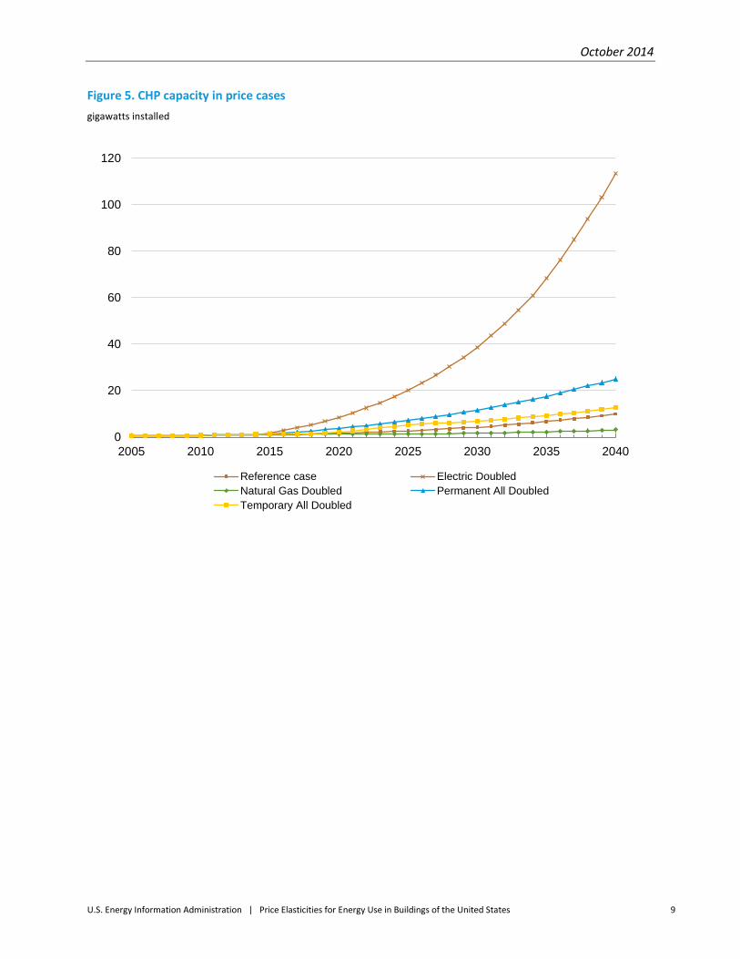
The largest-magnitude elasticity among all elasticity cases occurs in the commercial sector when natural gas consumption responds to an increasing electricity price (1.24). Much of this new natural gas consumption fuels increased combined heat and power (CHP) in the commercial sector.7 Figure 5 shows CHP capacity across the elasticity cases, growing at an average of 4.0% per year between 2014 and 2040 in the Natural Gas Price Doubled case, 8.6% per year in the Reference case, 9.7% in the Temporary All Fuel Prices Doubled case, 12.6% per year in the Permanent Prices Doubled case, and 19.3% per year in the Electricity Price Doubled case (CHP capacity in the Distillate Fuel Price Doubled case grows at the same pace as the Reference case). This dramatic increase in CHP in the Electricity Price Doubled case replaces natural gas used for other end uses, particularly space heating (see Figure 6)

7 CHP is generating equipment that provides electric power for a building and uses residual heat from that process for heating services. The buildings sectors use non-utility-scale CHP as a form of distributed generation (DG), a category of electricity generation that also includes renewables such rooftop solar and wind power systems at building locations. CHP is not very common in the residential sector; the significant increase in CHP takes place almost entirely in the commercial sector.

0

1

2

3

4

5

6

7

8

9

2010 2015 2020 2025 2030 2035 2040Reference case Permanent All DoubledNatural Gas Doubled Electricity DoubledDistillate Doubled

October 2014


Figure 5. CHP capacity in price cases gigawatts installed

0

20

40

60

80

100

120

2005 2010 2015 2020 2025 2030 2035 2040

Reference case Electric DoubledNatural Gas Doubled Permanent All DoubledTemporary All Doubled

October 2014


Figure 6. Natural gas consumption for space heating in the commercial sector quadrillion Btu

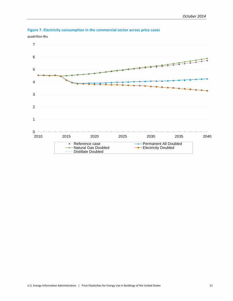
Energy demand: Electricity consumption and electric end uses in the Electricity Price Doubled case Figure 7 and Figure 8 show how electricity consumption changes in the price cases for the commercial and residential sectors, respectively. The largest drop in electricity consumption in both sectors is in the Electricity Price Doubled case. This case contains the highest combination of fuel switching from electricity and efficiency improvements in electricity end uses.

0.8

1.0

1.2

1.4

1.6

1.8

2.0

2005 2010 2015 2020 2025 2030 2035 2040

Reference case Electric DoubledNatural Gas Doubled Permanent All DoubledTemporary All Doubled

October 2014


Figure 7. Electricity consumption in the commercial sector across price cases quadrillion Btu

0

1

2

3

4

5

6

7

2010 2015 2020 2025 2030 2035 2040


October 2014


Figure 8. Electricity consumption in the residential sector across price cases quadrillion Btu

The primary methods for electricity fuel switching to occur are replacing electric equipment with equipment that runs on another fuel and increasing distributed generation (DG). Equipment switches may occur in the normal equipment life cycle, when an existing piece of equipment is due to be replaced, or they can happen before the lifetime of a piece of equipment has ended. Table 3 illustrates an example of fuel switching due to equipment stock changes, specifically heating equipment in the residential sector. The table presents the total number of units used for heating in households according to equipment types. Comparing heating equipment stocks between the cases shows that the Electricity Price Doubled case has many fewer electric heaters (particularly electric furnaces) and many more of the other technologies that use other fuels (particularly natural gas furnaces).

3.0

3.5

4.0

4.5

5.0

5.5

6.0

2010 2015 2020 2025 2030 2035 2040


October 2014


Table 3. Changes in residential heating equipment stock, 2040

Equipment Reference case Electricity Doubled Change*

Electric furnace 31,435,827 30,389,675 -1,046,152

Air-source heat pump (electric)

22,450,599 22,032,581 -418,018

Geothermal heat pump 2,424,993 2,319,999 -104,994

Natural gas furnace 61,305,282 62,693,721 +1,388,439

Natural gas boiler 10,427,291 10,483,002 +55,711

Natural gas heat pump 367,189 367,191 +2

Propane furnace 5,195,279 5,305,839 +110,560

Distillate furnace 1,836,483 1,845,937 +9,454

Distillate boiler 3,314,284 3,316,251 +1,967

Kerosene furnace 616,345 617,098 +753

Wood stove 2,428,022 2,430,309 +2,287

*Change from Reference case to Electricity Price Doubled case.

Increased use of DG at building sites is another form of fuel switching and also causes building occupants to use less electricity from central power plants. The previous section described the large increase in DG coming from CHP in the Electricity Price Doubled case, but DG also includes renewable sources at building sites such as rooftop solar panels and wind power systems. In the Electricity Price Doubled case, renewable DG grows 10.0% per year between 2014 and 2040, compared to 5.2% per year in the Reference case. The accelerated growth of renewable DG is not as fast as the accelerated growth of DG from CHP, but it still makes a significant impact on electricity consumption in the buildings sectors.

In addition to fuel switching, efficiency improvements also play a role in reducing electricity demand in the Electricity Price Doubled case. Most electric equipment experiences some efficiency improvements in the case, but the end uses that contribute the most to electricity savings are space cooling, lighting, and ventilation.

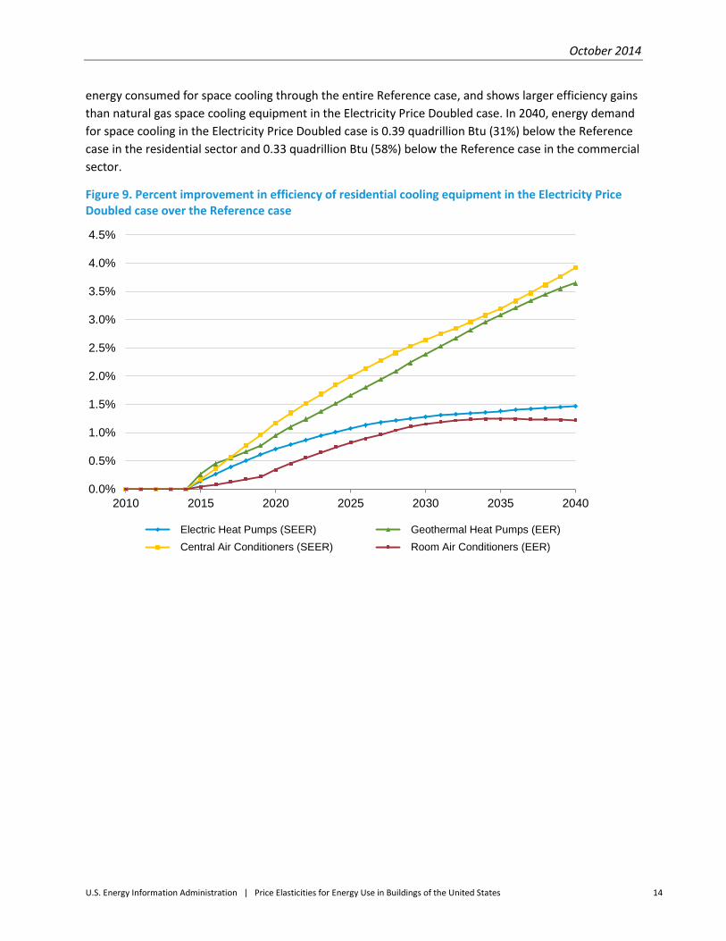
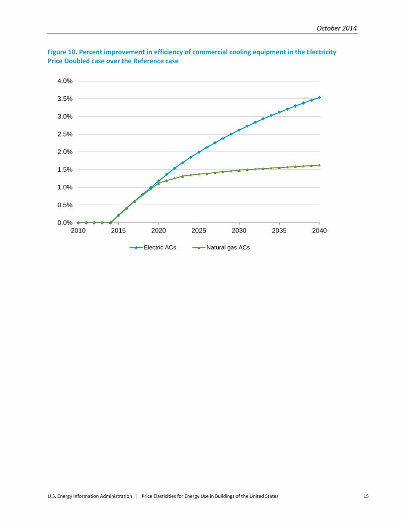
Figure 9 and Figure 10 show the efficiency improvements in residential space cooling equipment in the Electricity Price Doubled case compared to the Reference case. Central air conditioners and room air conditioners are the most prevalent space cooling equipment in the sector, accounting for 85% or more of household space cooling equipment through the entire Reference case and Electricity Price Doubled case.8 In the commercial sector, electric space cooling equipment accounts for more than 93% of the

8 The RDM also has a category for natural gas heat pumps that provide space cooling, but that was not included in Figure 8 because there was no efficiency improvement in that category in the Electricity Price Doubled case.

October 2014


energy consumed for space cooling through the entire Reference case, and shows larger efficiency gains than natural gas space cooling equipment in the Electricity Price Doubled case. In 2040, energy demand for space cooling in the Electricity Price Doubled case is 0.39 quadrillion Btu (31%) below the Reference case in the residential sector and 0.33 quadrillion Btu (58%) below the Reference case in the commercial sector.

Figure 9. Percent improvement in efficiency of residential cooling equipment in the Electricity Price Doubled case over the Reference case

0.0%

0.5%

1.0%

1.5%

2.0%

2.5%

3.0%

3.5%

4.0%

4.5%

2010 2015 2020 2025 2030 2035 2040

Electric Heat Pumps (SEER) Geothermal Heat Pumps (EER) Central Air Conditioners (SEER) Room Air Conditioners (EER)

October 2014


Figure 10. Percent improvement in efficiency of commercial cooling equipment in the Electricity Price Doubled case over the Reference case

0.0%

0.5%

1.0%

1.5%

2.0%

2.5%

3.0%

3.5%

4.0%

2010 2015 2020 2025 2030 2035 2040

Electric ACs Natural gas ACs

October 2014


In 2014, almost twice as much energy is consumed for lighting in the commercial sector as in the residential sector—0.90 quadrillion Btu versus 0.51 quadrillion Btu.9 In the Reference case, electricity demand for lighting declines faster in the residential sector than in the commercial sector, projecting 0.28 quadrillion Btu of electricity consumed for residential lighting and 0.84 quadrillion Btu of electricity consumed for commercial lighting in 2040.

In the Electricity Price Doubled case, savings in electricity consumption for lighting come from efficiency improvements that come mostly in the commercial sector. Energy use for lighting in the buildings sectors in this case is 0.64 quadrillion Btu (57%) below the Reference case in 2040, with 0.56 quadrillion Btu coming from the commercial sector. Figure 11 shows the amount of service demand for commercial lighting that different lighting technologies are projected to meet by 2040 in the Reference case and Electricity Price Doubled case.10 In the Electricity Price Doubled case, a higher share of commercial lighting demand is met with light-emitting diode (LED) technologies. LEDs produce less waste heat while producing light, which makes them much more efficient than other lighting options.

Figure 11. Lighting service demand for the commercial sector, Reference case vs. Electricity Price Doubled case lumen hours in trillions

While ventilation accounts for only a little over 7% of electricity consumption in the buildings sector, it still provides the third-largest amount of energy savings in the Electricity Price Doubled case. Savings in electricity use for ventilation come almost entirely from the commercial sector. In 2040, commercial sector ventilation energy use is 0.34 quadrillion Btu (56%) below the Reference case level in the

9 This result is the same in all cases presented, because price effects begin in 2015. 10 Service demand is not the same as energy demand. Service demand is a modeling concept meaning how much an end-user demands of a service (for example, lighting). The end-user then has to use energy-using equipment to fulfill that service demand (for example, light bulbs). Different types of equipment (for example, incandescent lighting, fluorescent lighting, LED lighting) may use different amounts of energy to meet service demand.

0

2000

4000

6000

8000

10000

12000

14000

Incandescent Fluorescent LED

Reference case Electricity Doubled

October 2014


Electricity Price Doubled case. This result stems from a much higher proportion of variable air volume (VAV) systems compared to constant air volume (CAV) systems to provide ventilation services in the Electricity Price Doubled case. Figure 12 shows the amount of service demand being met by VAVs and CAVs in the commercial sector in 2040. Since VAVs regulate the amount of air pumped based on room temperature conditions and CAVs only switch between a rest state and maximum output, VAVs are typically much more efficient.

Figure 12. Ventilation service demand for the commercial sector, Reference case vs. Electricity Price Doubled case Cubic feet per minute (CFM) hours in trillions

Costs in elasticity cases As shown in the preceding sections, price spikes cause changes in fuel consumption. This section examines the change in costs across the elasticity cases. Specifically, these costs include: fuels supplied to buildings energy consumers and the equipment and shell upgrades that take place in buildings.

Figure 13 presents total expenditures for all fuels supplied to consumers in the buildings sectors in the different cases. Even with the decreased energy usage presented earlier, total expenditures on fuels rise quite dramatically. This is expected because of the simulated doubling of fuel prices, but it is interesting to note the different levels of total fuel expenditures when different fuel prices rise. Compared to the Reference case, between 2015 and 2040 fuel expenditures increase by an average of $207 billion (2012 dollars) per year in the Electricity Price Doubled case, $157 billion per year in the Natural Gas Price Doubled case, and by $307 billion per year in the Permanent All Fuel Prices Doubled case. 11

11 For the Temporary All Fuel Prices Doubled case, total fuel expenditures increase above the Reference case by an average of $318 billion (2012 dollars) annually between 2020 and 2025.

0

50

100

150

200

250

300

350

CAV VAV

Reference case Electricity Doubled

October 2014


Figure 13. Total fuel expenditures for energy customers in price cases cost billion 2012 dollars

Figure 14 shows the costs for higher-efficiency equipment, DG systems, and residential shell improvements that occur across the cases.12 It combines what buildings energy consumers pay for the upgrades and also what the federal government pays through tax credit and subsidy programs as they exist in current legislation.

12 Results for investment in commercial building shells are not available.

300

400

500

600

700

800

900

1,000

2010 2015 2020 2025 2030 2035 2040

Reference case Temporary All Doubled Permanent All DoubledElectricity Doubled Natural Gas Doubled Distillate Doubled

October 2014


Figure 14. Consumer and government investment in equipment and shells across price cases cost billion 2012 dollars

Energy consumers pay a much higher share of the additional costs than the government for upgraded equipment and shells. In the Electricity Price Doubled case, the upgrades cost consumers an average of $22.5 billion per year more than the Reference case between 2015 and 2040 and cost the government an average of $0.6 billion more per year. In the Permanent Prices Doubled case, consumers pay an extra $18.0 billion per year, and government pays an extra $0.6 billion per year.

150

160

170

180

190

200

210

220

230

240

2010 2015 2020 2025 2030 2035 2040

Reference case Temporary All Doubled Permanent All Doubled Electricity Doubled

October 2014


Conclusion The three possible responses for an energy user to counter an increase in the cost of a particular fuel are to switch to another fuel, to use that fuel more efficiently, or to not use that fuel. Whether one option is more desirable than another, or even possible, depends on many factors. For example, lighting demand is powered almost entirely through electricity, and there is no general service lighting that runs on natural gas. Thus, an increase in electricity price will not cause fuel switching in lighting, but it may persuade building occupants to purchase more-efficient light bulbs or to be more aware of turning off lights when they are not needed.

There is no way to know the future price of anything, but the simulations described above provide a range of possibilities to help understand price-demand dynamics, particularly for the buildings sectors. Electricity and natural gas are the most important fuels in the buildings sectors. In the Reference case, electricity accounts for 47% of delivered energy in 2014 and grows to 54% in 2040. The share of natural gas is slightly lower and declines over the course of the Reference case, but accounts for 41% of delivered energy in 2014 and 37% in 2040. It is likely because of the high and growing use of electricity that elasticities are larger when the electricity price is doubled than when other energy prices are doubled. These interactions, along with the other changes described above by fuel price increases, help in understanding energy consumption and in planning for future energy needs.

October 2014


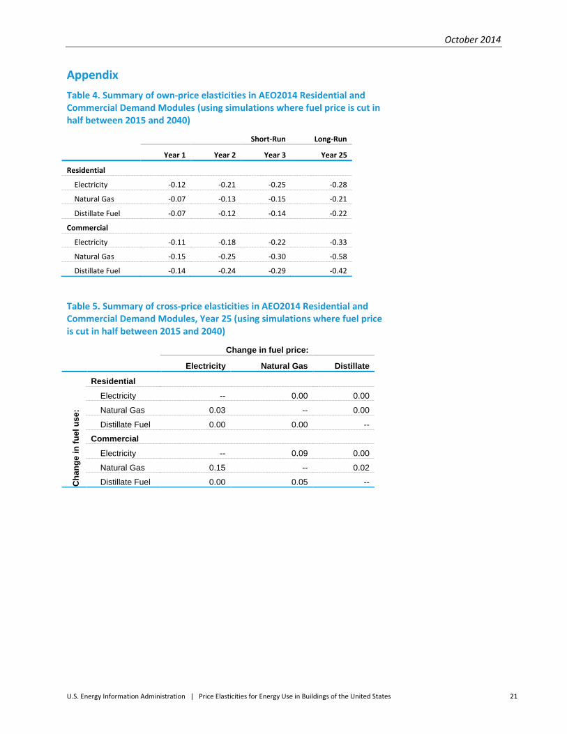
Appendix Table 4. Summary of own-price elasticities in AEO2014 Residential and Commercial Demand Modules (using simulations where fuel price is cut in half between 2015 and 2040)

Short-Run Long-Run

Year 1 Year 2 Year 3 Year 25

Residential

Electricity -0.12 -0.21 -0.25 -0.28

Natural Gas -0.07 -0.13 -0.15 -0.21

Distillate Fuel -0.07 -0.12 -0.14 -0.22

Commercial

Electricity -0.11 -0.18 -0.22 -0.33

Natural Gas -0.15 -0.25 -0.30 -0.58

Distillate Fuel -0.14 -0.24 -0.29 -0.42

Table 5. Summary of cross-price elasticities in AEO2014 Residential and Commercial Demand Modules, Year 25 (using simulations where fuel price is cut in half between 2015 and 2040)

Change in fuel price:

Electricity Natural Gas Distillate

Cha

nge

in fu

el u

se:

Residential




Commercial




Price Elasticities for Energy Use in Buildings of the ... · Price Elasticities for Energy Use in...

Documents

Transcript of Price Elasticities for Energy Use in Buildings of the ... · Price Elasticities for Energy Use in...