Price Discrimination in International Airline Markets

Price Discrimination in International Airline Markets∗

Gaurab Aryal† Charles Murry‡ Jonathan W. Williams§

February 22, 2021

Abstract

We develop a model of inter-temporal and intra-temporal price discrimination bymonopoly airlines to study the ability of different discriminatory pricing mechanismsto increase efficiency and the associated distributional implications. To estimate themodel, we use unique data from international airline markets with flight-level varia-tion in prices across time, cabins, and markets, as well as information on passengers’reasons for travel and time of purchase. We find that the ability to screen passengersacross cabins every period increases total surplus by 35% relative to choosing only oneprice per period, with both the airline and passengers benefiting. However, furtherdiscrimination based on passenger’s reason to traveling improve airline surplus at theexpense of total efficiency. We also find that the current pricing practice yields ap-proximately 89% of the first-best welfare. The source of this inefficiency arises mostlyfrom dynamic uncertainty about demand, not private information about passengervaluations.

∗We are very grateful to the U.S. Department of Commerce for providing the data for our analysis.We are thankful to research computing facilities at Boston College, UNC and UVA, with special thanks toSandeep Sarangi at UNC research computing. Seminar (Arizona, BC, MIT, Penn State, Rice, Richmond Fed,Rochester, Texas A&M Toulouse, UC-Irvine, UNC-Chapel Hill, UWO, UWSTL, Vanderbilt, Virginia) andconference (SEA 2014, EARIE 2015, IIOC 2016, ASSA 2016, DSE 2019, SITE 2019) participants providedhelpful comments. We thank Jan Brueckner, Ben Eden, Gautam Gowrisankaran, Jacob Gramlich, QihongLiu, Brian McManus, Nancy Rose, Nick Rupp for insightful suggestions. All remaining errors are our own.

†Department of Economics, University of Virginia, [email protected].‡Department of Economics, Boston College, [email protected].§Department of Economics, University of North Carolina - Chapel Hill, [email protected].

1

Electronic copy available at: https://ssrn.com/abstract=3288276

1 IntroductionFirms with market power often use discriminatory prices to increase their profits. However,such price discrimination can have ambiguous implications on total welfare. Enhanced pricediscrimination may increase welfare by reducing allocative inefficiencies but may also reduceconsumer welfare. So, an essential aspect of economic- and public-policy towards pricediscrimination is to understand how well various discriminatory prices perform in terms ofthe total welfare and its distribution, relative to each other and the first-best, (e.g., Pigou,1920; Varian, 1985; Council of Economic Advisors, 2015).

We evaluate the welfare consequences of price discrimination and quantify sources ofinefficiencies in a large and economically important setting, international air travel mar-kets. To that end, we develop and estimate a model of inter-temporal and intra-temporalprice discrimination by a monopoly airline and study the ability of different discriminatorymechanisms to increase welfare and the associated distributional implications. The modelincorporates a rich specification of passenger valuations for two vertically differentiated seatclasses on international flights, and a capacity-constrained airline that faces stochastic andtime-varying demand. The airline screens passengers between two cabins while updatingprices and seat offerings over time. Using the model estimates, we implement various coun-terfactuals in the spirit of Bergemann, Brooks, and Morris (2015), where we change theinformation the airline has about preferences and the timing of arrivals and measure thewelfare under various discriminatory pricing strategies. Our counterfactual pricing strate-gies are motivated by recent airline practices intended to raise profits by reducing allocativeinefficiencies, including attempts to solicit passengers’ reason to travel and use of auctions(e.g., Nicas, 2013; Vora, 2014; Tully, 2015; McCartney, 2016).

We find that the ability to screen passengers across cabins increases the total surplusby 35% relative to choosing a single price each period (i.e., “shutting down” second-degreeprice discrimination across cabins), with both airline and passengers benefiting. However,further discriminatory practices based on passengers’ reason to travel improve the airline’ssurplus but lower the total surplus. We also find that the current pricing practice yieldsapproximately 89% of the first-best welfare, and that the source of this remaining inefficiencyis mostly due to the dynamic uncertainty about demand, not the private information aboutpassengers’ valuations.1 This suggests that airlines’ attempts to improve dynamic allocationscould provide efficiency improvements.

Our empirical strategy centers around a novel dataset of international air travel from the1 Here, the “first-best” welfare is defined in the context of our model. There may be other effects worth

exploring, for example ticket resale in Lazarev (2013), that our model does not capture.

2


U.S. Department of Commerce’s Survey of International Air Travelers. Compared to theextant literature, the novelty of these data is that we observe both the date of transactionsand passenger characteristics for dozens of airlines in hundreds of markets. We document thelate arrival of passengers traveling for business, who tend to have inelastic demand, and theassociated changes in prices. Although business travelers’ late arrival puts upward pressureon fares, fares do not increase monotonically for every flight. This pattern suggests that theunderlying demand for air travel is stochastic and non-stationary.

To capture these salient data features, we propose a flexible but tractable demand system.Each period before a flight departs, a random number of potential passengers arrive andpurchase a first-class ticket, an economy class ticket, or decide not to fly at all. Passengers’willingness-to-pay depends on the seat class and passenger’s reason to travel. We allowpassengers to have different willingness-to-pay for first-class, so, for some passengers, thetwo cabins are close substitutes but not for others. Furthermore, we allow the mix of thetwo types of passengers–business and leisure–to vary over time.

On the supply side, we model a monopoly airline’s problem of selling a fixed number ofeconomy and first-class seats. The airline knows the distribution of passengers’ valuationsand the expected number of arrivals each period but chooses prices and seats to release beforeit realizes actual demand.2 At any time before the flight, the airline balances expected profitfrom selling a seat today against the forgone future expected profit. This inter-temporaltrade-off results in a time-specific endogenous opportunity cost for each seat that varies withthe expected future demand and number of unsold seats. Besides this temporal consideration,each period, the airline screens passengers between the two cabins. Thus, our model capturesboth the inter-temporal and intra-temporal aspects of price discrimination by airlines.

Estimation of our model presents numerous challenges. The richness of the demand,and our supply specification, result in a non-stationary dynamic programming problem thatinvolves solving a mixed-integer nonlinear program for each state. We solve this problemto determine optimal prices and seat-release policies for each combination of unsold seatsand days until departure. Moreover, our data include hundreds of flights across hundreds ofroutes, so not only do we allow for heterogeneity in preferences across passengers within aflight, we also allow different flights to have different distributions of passenger preferences.To estimate the model and recover the distribution of preferences across flights, we use asimulated method of moments approach based on Ackerberg (2009). Similar approachesto estimate a random coefficient specification has recently been used by Fox, Kim, andYang (2016), Nevo, Turner, and Williams (2016), and Blundell, Gowrisankaran, and Langer

2 We model the airline committing to a seat release policy to mimic the “fare bucket” strategy used byairlines in practice. See, for example, Alderighi, Nicolini, and Piga (2015) for more on these buckets.

3


(2020). Like these papers, we match empirical moments describing within-flight and across-flight variation in fares and purchases to a mixture of moments implied by our model.

Our estimates suggest that there is substantial heterogeneity across passengers withina flight and substantial heterogeneity across flights. The estimated marginal distributionsof willingness-to-pay for business and leisure travelers are consistent with the observed dis-tribution of fares. We estimate that the average willingness-to-pay for an economy seat inour data by leisure and business passengers is $413 and $506, respectively. Furthermore, onaverage, passengers value a first-class seat 23% more than an economy seat, which impliesmeaningful cross-cabin substitution. We also find declining arrivals of passengers overall, butwith an increasing fraction of business travelers. Using the model estimates, we calculatethe unobserved time-varying opportunity cost of selling a seat, which provides novel insightinto airlines’ dynamic incentives.

Using the estimates and the model, we characterize the level of efficiency and the associ-ated distribution of surplus for alternative pricing mechanisms that provide new insights onthe welfare consequences of price discrimination. In terms of efficiency, we find that airlines’current pricing practices increase total welfare by 35%, compared to a scenario where weprohibit airlines from charging multiple prices across cabins. We also find that the currentpricing achieves 89% of the first-best welfare, and almost all of this inefficiency is due to theuncertainty about passengers’ arrivals. However, greater discrimination based on the reasonto travel –business versus leisure– improves airlines’ surplus but slightly lowers total surplus.

In terms of the surplus distribution between airlines and passengers, we find that pricediscrimination skews the distribution of surplus in favor of the airlines. In particular, thegap between producer surplus and consumer surplus increases by approximately 37% whenairlines price differently across cabins, compared to setting only one price per period. Addi-tional price discrimination based on passengers’ reasons to travel or willingness-to-pay leadsto a higher airline surplus but a lower total surplus. We illustrate this “monopoly external-ity” by determining surplus division when the airline uses a Vickery-Clarke-Grove (VCG)auction, period-by-period. We find that using VCG more than doubles the consumer sur-plus, compared to the current pricing practices, while still achieving the same efficiency aseliminating all static informational frictions.

Contribution and Related Literature. Our paper relates to a vast research on theeconomics of price discrimination and research in the empirical industrial organization onestimating the efficiency and division of welfare under asymmetric information. Most of theseempirical papers focus on either cross-sectional price discrimination (e.g., Ivaldi and Mar-timort, 1994; Leslie, 2004; Busse and Rysman, 2005; Crawford and Shum, 2006; McManus,

4


2007; Aryal and Gabrielli, 2019) or inter-temporal price discrimination dynamics (e.g., Nevoand Wolfram, 2002; Nair, 2007; Escobari, 2012; Jian, 2012; Hendel and Nevo, 2013; Lazarev,2013; Cho et al., 2018; Kehoe, Larsen, and Pastorino, 2020).

There is also a literature that focuses on dynamic pricing (e.g., Graddy and Hall, 2011;Sweeting, 2010; Cho et al., 2018; Williams, 2020). However, none study intra-temporalprice discrimination, inter-temporal price discrimination and dynamic pricing together, eventhough many industries involve all three. We contribute to this research by developing anempirical framework where both static discriminative pricing and dynamic pricing incentivesare present and obtain results that characterize the welfare implications.3

Additionally, we complement recent research related specifically to airline pricing, partic-ularly Lazarev (2013), Li, Granados, and Netessine (2014), and Williams (2020).4 Lazarev(2013) considers a model of inter-temporal price discrimination with one service cabin andfinds large potential gains from allowing reallocation among passengers arriving at differenttimes before the flight (through ticket resale). Williams (2020) further allows for dynamicadjustment of prices in response to stochastic demand and finds that dynamic pricing (rel-ative to a single price) increases total welfare at the expense of business passengers. Li,Granados, and Netessine (2014) use an instrumental variables strategy to study strategicbehavior of passengers and infer that between 5% and 20% of passengers wait to purchasein a sample of domestic markets, with the share decreasing in market distance.5 Incor-porating this strategic consumer behavior into a structural model of pricing like Lazarev(2013), Williams (2020), and ours remains unexplored due to theoretical and computationaldifficulties, although Lazarev (2013) allows passengers to cancel their ticket.

Building on Lazarev (2013) and Williams (2020), we allow the airline to manage revenueby optimally choosing the number of seats to release and by screening passengers betweentwo cabins. Through counterfactuals, our approach allows us to measure the importance ofdifferent channels through which inefficiencies arise in airline markets. In terms of estimation,we also allow a rich specification for unobserved heterogeneity across markets via a randomcoefficients approach to estimation. The richness of random coefficients allows us capturevariation in demand parameters due to permanent and unobserved differences across markets.

3 There is a long and active theoretical literature on static and inter-temporal price discrimination, seeStokey (1979); Gale and Holmes (1993); Wilson (1993); Dana (1999); Courty and Li (2000); Armstrong(2006) and references therein. Airline pricing has also been studied extensively from the perspective ofrevenue management; see van Ryzin and Talluri (2005).

4 Relatedly, Borenstein and Rose (1994), Puller, Sengupta, and Wiggins (2012); Chandra and Lederman(2018) use a regression approach to study effects of oligopoly on price dispersion and price discrimination inairline markets.

5 We expect the share to be small in our context because we study long-haul international markets.

5


2 DataThe Department of Commerce’s Survey of International Air Travelers (SIAT) gathers infor-mation on international air passengers traveling to and from the U.S. Passengers are askeddetailed questions about their flight itinerary, either during the flight or at the gate areabefore the flight. The SIAT targets both U.S. residents traveling abroad and non-residentsvisiting the U.S. Passengers in our sample are from randomly chosen flights from amongmore than 70 participating U.S. and international airlines, including some charter carriers.The survey contains ticket information, which includes the cabin class (first, business, oreconomy), date of purchase, total fare, and the trip’s purpose (business or leisure). Wecombine fares that are reported as business class and first-class into a single cabin class thatwe label “first-class.” This richness distinguishes the SIAT data from other data like theOrigin and Destination Survey (DB1B) conducted by the Department of Transportation. Inparticular, the additional detail about passengers (e.g., time of purchase, individual ticketfares, and reason for travel) make the SIAT dataset ideal for studying price discrimination.

We create a dataset from the survey where a unit of observation is a single ticket pur-chased by a passenger flying a nonstop (or direct) route. We then use fares and purchase(calendar) dates associated with these tickets to estimate “price paths” for each flight in ourdata, where a flight is a single instance of a plane serving a particular route. For example,in our sample, we observe some nonstop passengers flying United Airlines from SEA to TPEon August 12, 2010, departing at 5:10 pm, then we say that this is one flight. From thedata on fares and dates for this flight, we use kernel regression to estimate price paths foreconomy seats and first-class seats leading up to August 12, 2010. In this section, we detailhow we selected the sample and display descriptive statistics that motivate our model andanalysis.

2.1 Sample Selection

Our sample from the DOC includes 413,309 passenger responses for 2009-2011. We clean thedata in order to remove contaminated and missing observations and to construct a sample offlights that will inform our model of airline pricing which we specify in the following section.We detail our sample selection procedure in Appendix A.1, but, for example, we excluderesponses that do not report a fare, are part of a group travel package, or are non-revenuetickets. We supplement our data with schedule data from the Official Aviation Guide of theAirways (OAG) company, which reports cabin-specific capacities, by flight number. Usingthe flight date and flight number in SIAT we can merge the two data sets. We include flightsfor which we observe at least ten nonstop tickets after applying the sample selection criteria.

6


Nonstop Markets and Capacity. Like other studies that model discriminatory pricingby airlines (e.g., Lazarev (2013); Puller, Sengupta, and Wiggins (2012); Williams (2020)),we focus on nonstop travel in monopoly markets, where we define monopoly market criteriabelow. Although a physical flight will have both connecting and nonstop passengers, weassume that an airline devotes a specific portion of a plane to nonstop passengers before itstarts selling tickets, and the airline does not change the plane’s apportionment. We makethis assumption to keep our model tractable because modeling airlines’ pricing strategies forboth nonstop and connecting passengers is a high-dimensional optimization problem thathas to balance the cross-elasticities of passengers on all potential itineraries in the airline’snetwork that could use one of the flights in our sample as a leg.

Specifically, we determine the ratio of nonstop travel on a flight in our survey by firstdetermining the ratio of nonstop travel for the route in a quarter from the Department ofTransportation’s DB1B data. We then apply this ratio to the total capacity of the equipmentused (which we observe and we describe below) in our sample to arrive at a nonstop capacityfor each flight. As an illustration, consider the SEA to TPE flight on August 12, 2010.Suppose in this flight, United Airlines used a Boeing 757 with 235 economy seats, andaccording to the DB1B data in Q3:2010, only 45 percent of tickets for this market arenonstop tickets. Then, for us, this means that United Airlines reserved only 110 economyseats (out of 235) for nonstop travel, and so the initial economy class capacity for this flightmarket is 110. We repeat this exercise for the first-class seats.6

We observe the entire itinerary of a passenger, so to select ticket purchases for our finalsample, we discard all passengers using a flight as part of a connecting itinerary. For example,if we see a passenger report flying from Cleveland to Taipei via Seattle, we drop them fromour sample. The same is true if we observe a passenger flying from Toulouse to Charlottevia Paris.

“Monopoly” Markets. As mentioned earlier, we focus on monopoly markets. In inter-national air travel, nonstop markets tend to be concentrated for all but the few busiestairport-pairs. We classify a market as a monopoly-market if it satisfies one of followingtwo criteria: (i) one airline flies at least 95% of the total capacity on the route (where thecapacity is measured using the OAG data); or (ii) there is a US carrier and foreign carrierthat operate on the market with antitrust immunity from the U.S. Department Of Justice.

These antitrust exemptions come from market access treaties signed between the U.S.and the foreign country that specify a local foreign carrier (usually an alliance partner of theU.S. airline) that will share the route. For example, on July 20, 2010 antitrust exemption

6 Few flights are not in the DB1B dataset, and for them, we use the nonstop ratio from the SIAT survey.

7


was granted to OneWorld alliance, which includes American Airlines, British Airways, Iberia,Finnair and Royal Jordanian, for 10 years subject to a slot remedy.7

In a few cases, we define markets at the city-pair level because we are concerned thatwithin-city airports are substitutable. The airports that we aggregate up to a city-pairsmarket definition include airports in the New York, London, and Tokyo metropolitan. Thus,we treat a flight from New York JFK to London Heathrow to be in the same market as aflight from Newark EWR to London Gatwick.

Table 1: Top 20 Markets, ordered by sample representation

Unique Distance Unique DistanceMarket Flights Obs. (miles) Market Flights Obs. (miles)LAX-PVG 53 1,060 6,485 JFK-SCL 16 239 5,096JFK-HEL 35 581 4,117 SFB-BHX 10 234 4,249SFO-AKL 28 497 6,516 JFK-NCE 9 217 3,991JFK-VIE 29 469 4,239 PHX-SJD 15 211 721JFK-EZE 24 444 5,281 JFK-POS 13 208 2,204JFK-WAW 34 434 4,267 JFK-PLS 8 205 1,303JFK-JNB 26 368 7,967 SFO-HND 4 198 5,161JFK-CCS 20 360 2,109 BOS-KEF 12 178 2,413JFK-CMN 21 330 3,609 SFO-CDG 10 162 5,583SEA-TPE 21 328 6,074 JFK-MTY 9 148 1,826

Note: The table displays the Top 25 markets, their representation in our sample, their distance (air miles)from U.S. Data from the Survey of International Air Travelers and sample described in the text.

Description of Markets and Carriers. After our initial selection and restriction onnonstop monopoly markets, we have 14,930 observations representing 224 markets and 64carriers. We list the top 20 markets based on sample representation in Table 1, along withthe number of unique flights and the total observations. The most common U.S. airports inour final sample are San Francisco (SFO), New York JFK (JFK), and Phoenix (PHX), andthe three most common routes are SFO to Auckland, New Zealand (AKL), JFK to Helsinki,Finland (HEL), and JFK to Johannesburg, South Africa (JNB). The median flight has adistance of 4,229 miles, and the inter-quartile range of 2, 287 to 5, 583 miles. In Table 2 wedisplay the top ten carriers from our final sample, which represent approximately 60% of ourfinal observations.

2.2 Passenger Arrivals and Ticket Sale Process

Passengers differ in terms of time of purchases and reasons for travel and prices vary overtime and across cabins. In this subsection we present key features in our data pertaining the

7 To determine such markets, we use information from DOT and carriers’ 10K reports filed with the SEC.

8


Table 2: Top Ten Carriers, ordered by sample representation

Carrier Unique Flights Obs.American Airlines 88 1526Continental 98 1483US Airways 72 1200Eastern China 53 1060Finnair 35 581Austrian 35 573Lufthansa 40 558Delta 35 550Air New Zealand 30 520ThomsonFly 20 470

Note: The table displays the top ten carriers, ordered by their frequency in the final sample. Data fromthe Survey of International Air Travelers and sample described in the text.

passengers and prices.

Timing of Purchase. Airlines typically start selling tickets a year before the flight date.Although passengers can buy their tickets throughout the year, in our sample most passengersbuy in the last 120 days. To keep the model and estimation tractable, we classify the purchaseday into a fixed number of bins. There are at least two factors that motivate our choice ofbin sizes. First, it appears that airlines typically adjust fares frequently in the last few weeksbefore the flight date, but less often farther away from the flight date. Second, there isusually a spike in passengers buying tickets at focal points, like 30 days, 60 days etc. InTable 3 we present eight fixed bins, and the number of observations in each bin, and as wecan see we use narrower bins when we are closer to the flight date. Each of these eight binscorrespond to one period, giving us a total of eight periods.

Passenger Characteristics. We classify each passenger as either a business traveler ora leisure traveler based on the reason to travel. Business includes business, conference,and government/military, while leisure includes visiting family, vacation, religious purposes,study/teaching, health, and other, see Table A.1.1 for more.8 We classify service cabins intoeconomy class and first-class, where we classify every premium service cabin as latter.

In Table 4 we display some key statistics for relevant ticket characteristics in our sample.As is common in the literature, to make one-way and round-trip fares comparable we divideround-trip fares by two. Approximately 4.5% passengers report to have bought a one-way

8 We also observe the channel through which the tickets were purchased: travel agents (36.47%), personalcomputer (39.76%), airlines (13.36%), company travel department (3.99%), and others (6.42%).

9


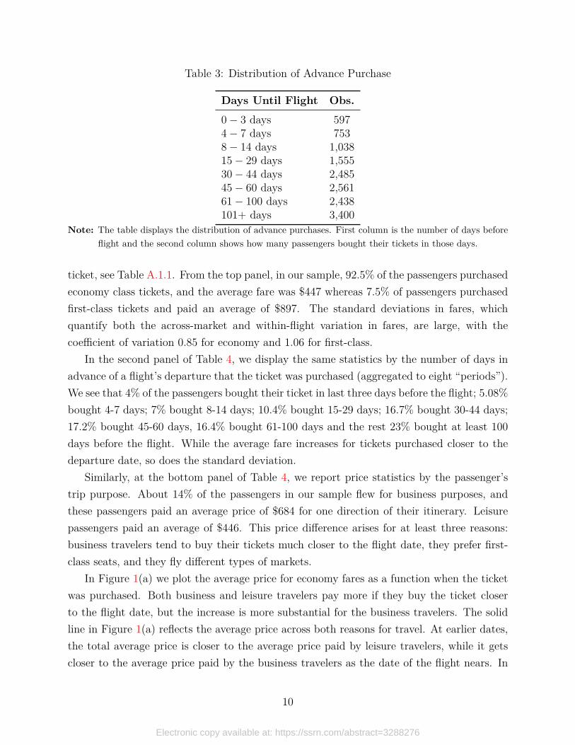
Table 3: Distribution of Advance Purchase

Days Until Flight Obs.0− 3 days 5974− 7 days 7538− 14 days 1,03815− 29 days 1,55530− 44 days 2,48545− 60 days 2,56161− 100 days 2,438101+ days 3,400

Note: The table displays the distribution of advance purchases. First column is the number of days beforeflight and the second column shows how many passengers bought their tickets in those days.

ticket, see Table A.1.1. From the top panel, in our sample, 92.5% of the passengers purchasedeconomy class tickets, and the average fare was $447 whereas 7.5% of passengers purchasedfirst-class tickets and paid an average of $897. The standard deviations in fares, whichquantify both the across-market and within-flight variation in fares, are large, with thecoefficient of variation 0.85 for economy and 1.06 for first-class.

In the second panel of Table 4, we display the same statistics by the number of days inadvance of a flight’s departure that the ticket was purchased (aggregated to eight “periods”).We see that 4% of the passengers bought their ticket in last three days before the flight; 5.08%bought 4-7 days; 7% bought 8-14 days; 10.4% bought 15-29 days; 16.7% bought 30-44 days;17.2% bought 45-60 days, 16.4% bought 61-100 days and the rest 23% bought at least 100days before the flight. While the average fare increases for tickets purchased closer to thedeparture date, so does the standard deviation.

Similarly, at the bottom panel of Table 4, we report price statistics by the passenger’strip purpose. About 14% of the passengers in our sample flew for business purposes, andthese passengers paid an average price of $684 for one direction of their itinerary. Leisurepassengers paid an average of $446. This price difference arises for at least three reasons:business travelers tend to buy their tickets much closer to the flight date, they prefer first-class seats, and they fly different types of markets.

In Figure 1(a) we plot the average price for economy fares as a function when the ticketwas purchased. Both business and leisure travelers pay more if they buy the ticket closerto the flight date, but the increase is more substantial for the business travelers. The solidline in Figure 1(a) reflects the average price across both reasons for travel. At earlier dates,the total average price is closer to the average price paid by leisure travelers, while it getscloser to the average price paid by the business travelers as the date of the flight nears. In

10


Table 4: Summary Statistics from SIAT, Ticket Characteristics

Proportion FareTicket Class of Sample Mean S.D.Economy 92.50 447 382First 7.50 897 956

Advance Purchase0-3 Days 4.03 617 6364-7 Days 5.08 632 6798-14 Days 7.00 571 59915-29 Days 10.49 553 56730-44 Days 16.76 478 42945-60 Days 17.27 467 43261-100 Days 16.44 414 315101+ Days 22.93 419 387

Travel PurposeLeisure 85.57 446 400Business 14.43 684 716

Note: Data from the Survey of International Air Travelers. Sampledescribed in the text.

Figure 1: Business versus Leisure Passengers before the Flight Date

01234567891011121314151617400

450

500

550

600

(a) Average Economy Fares Prior to Flight

012345678910111213141516170

0.05

0.1

0.15

0.2

0.25

0.3

0.35

(b) Business and Leisure Travelers

Note: (a) Average price paths across all flights for tickets in economy class by week of purchase prior tothe flight date, by self-reported business and leisure travelers. Individual transaction prices are smoothedusing nearest neighbor with a Gaussian kernel with optimal bandwidth of 0.5198. (b) Proportion ofbusiness passengers across all flights, by advance purchase weeks.

11


Figure 1(b), we display the proportion of business to leisure travelers across all flights, by theadvance purchase categories. In the last two months before flight, the share of passengerstraveling for leisure is approximately 90%, which decreases to 65% a week before flight.Taken together, business travelers purchase closer to the flight date than leisure travelers,and markets with a greater proportion of business travelers have a steeper price gradient.

Figure 2: Histogram of Percent of Business Passengers by Flight

Note: Histogram of business-travel index (BTI). The business-traveler index is the flight-specific ratio ofself-reported business travelers to leisure travelers. The mean is 0.154 and the standard deviation is 0.210.

Observing the purpose of travel plays an important role in our empirical analysis, reflect-ing substantial differences in the behavior and preferences of business and leisure passengers.This passenger heterogeneity across markets drives variation in pricing, and this covariationpermits us to estimate a model with richer consumer heterogeneity than the existing liter-ature like Berry, Carnall, and Spiller (2006) and Ciliberto and Williams (2014). Further, aclean taxonomy of passenger types allows a straightforward exploration of the role of asym-metric information in determining inefficiencies and the distribution of surplus that arisesfrom discriminatory pricing of different forms.9

To further explore the influence that this source of observable passenger heterogeneityhas on fares, we present statistics on across-market variation in the dynamics of fares. Specif-ically, we first calculate the proportion of business travelers in each market, i.e., across allflights with the same origin and destination. Like Borenstein (2010), we call this market-

9 In the raw data, 5.46% of passengers report that the main reason why they choose their airline isfrequent flyer miles. In our final (estimation) sample, 1.7% passengers get upgraded, i.e., they buy economybut fly first-class. Our working hypothesis is that those upgrades materialized only on the day of travel.

12


specific ratio the business-traveler index (BTI). In Figure 2, we present the histogram of theBTI across markets in our data. If airlines know of this across-market heterogeneity anduse it as a basis to discriminate both intra-temporally (across cabins) and inter-temporally(across time before a flight departs), different within-flight temporal patterns in fares shouldarise for different values of the BTI.

Figure 3: Proportion of Business Travelers by Ticket Class

(a) Economy Class (b) First-Class

Note: The figure presents kernel regression of reason to travel on BTI and the purchase date. Panels (a)and (b) show the regression for economy and the first-class seats, respectively. The regression uses aGaussian with optimal ‘rule-of-thumb’ bandwidth.

In Figure 3 we present the results of a bivariate kernel regression where we regress anindicator for whether a passenger is traveling for business on the BTI in that market andnumber of days the ticket was purchased in advance of the flight’s departure. Figures 3(a)and 3(b) present the results for economy and first-class passengers, respectively. There aretwo important observations. First, across all values of the BTI, business passengers arrivelater than leisure passengers. Second, business passengers disproportionately choose first-class seats. To capture this feature, in Section 3, we model the difference between businessand leisure passengers in terms of the timing of purchases and the preference for qualityby allowing the passenger mix to change as the flight date approaches, resulting in a non-stationary demand process.

The influence of business passengers is evident on prices. Like Figure 3, Figure 4(a)and Figure 4(b) present the results of a kernel regression with fare paid as the dependentvariable for economy and first-class cabins, respectively. In both, we present cross-sectionsof these estimated surfaces for the 25th, 50th, and 75th percentile values of the BTI. For bothcabins, greater values of the BTI are associated with substantially higher fares. Further,

13


Figure 4: Across-Market Variation in Fares

0 10 20 30 40 50 60 70360

380

400

420

440

460

480

500

520

540

(a) Economy

0 10 20 30 40 50 60 70600

700

800

900

1000

1100

1200

(b) First-Class

Note: The figure presents results from a kernel regression of fares paid on BTI and the purchase date.Panels (a) and (b) show the results from the regression evaluated at different values of BTI, for economyand the first-class seats, respectively. The regression uses a Gaussian with optimal ‘rule-of-thumb’bandwidth.

there is a positive relationship between the rate of increase as the flight date approachesand the BTI, and this rate is positive as the flight date approaches only in markets withnon-zero BTI. This pattern is most evident in first-class fares. Thus, the presence of businesstravelers is associated with both greater average fares and steeper increases in fares as theflight date approaches for both cabins. The larger increase in first-class fares as the flightdate approaches, relative to economy fares, is consistent with the strong selection of businesstravelers into the first-class cabin.

While there are clear patterns in how the dynamics of average fares vary with the BTI,there is also substantial heterogeneity across flights in how fares change as the flight dateapproaches. To see the heterogeneity in temporal patterns for individual flights that Fig-ure 3 masks, Figure 5 presents the time-paths of economy fares for all flights in our data.Specifically, for each flight, we estimate a smooth relationship between economy fares andtime before departure using a kernel regression, and then normalize the path relative to theinitial fare for that flight. Each line is a single flight from our data, and begins when we firstobserve a fare for that flight, and ends at 1, the day of the flight.

For most flights we observe little movement in fares until approximately 100 days beforedeparture. Yet, for a small proportion of flights, there are substantial decreases and increasesin fares as much as 5 months before departure. Further, by the date of departure, theinterquartile range of the ratio of current fare to initial fare is 0.75 to 1.85. Thus, 25% of

14


Figure 5: Flight-Level Dispersion in Fares

Note: The figure presents the estimated fare paths from every flight we use in our estimation. Each linerepresents a flight. We normalize the fares to unity by dividing fares by the first fare we observe for theflight. The horizontal axis represents the number of days until the flight, where zero is the flight date.

flights experience a decrease of more than 25%, while 25% of flights experience an increase ofgreater than 85%. The variation in the temporal patterns in fares across flights is attributableto both the across-market heterogeneity in the mix of passengers, and how airlines respondto demand uncertainty.

2.3 Aircraft Characteristics

Airlines’ fares, and their responsiveness to realized demand, depend on the number of unsoldseats. In Figure 6(a) we display the joint density of initial capacity of first and economyclass in our sample. The median capacity of an aircraft in our sample is 116 economy seatsand 15 first-class seats, and the mode is 138 economy and 16 first-class seats.

The three most common aircraft types in our sample are a Boeing 777, 747, and 737(36% of flights in our sample). The 777 and 747 are wide-body jets. The 777 has a typicalseating of around 350 seats and the 737 has a typical seating of around 160 seats (beforeadjusting for non-stop versus connecting passengers). The most common Airbus equipmentis the A330, which makes up about 4% of the flights in our sample.

Across all flights, on average 88% of all seats are economy class. We merge the SIAT datawith the Department of Transportation’s T-100 segment data to get a measure of the loadfactor for our SIAT flights. From the T100, we know the average load factor across a monthfor a particular route flown by a particular type of equipment. In Figure 6(b) we display thedensity of load factor across flights in our sample. The median load factor is 82%, but thereis substantial heterogeneity across flights.

15


Figure 6: Initial Capacity and Load Factor

(a) Density of Initial Capacities (b) Histogram of Load Factor

Note: In part (a) this figure presents the Parzen-Rosenblatt Kernel density estimate of the joint-density ofinitial capacities available for nonstop travel. In part (b) this figure presents the histogram of the passenger

load factor across our sample.

Overall, our descriptive analysis reveals a number of salient features that we capturein our model. We find that a business-leisure taxonomy of passenger types is useful tocapture differences in the timing of purchase, willingness-to-pay, and preference for quality.Further, we find substantial heterogeneity in the business or leisure mix of passengers acrossmarkets, which airlines are aware of and responsive to, creating variation in both the leveland temporal patterns of fares across markets. Finally, across flights we observe considerableheterogeneity in fare paths as the flight date approaches. Together, these features motivateour model of non-stationary and stochastic demand and dynamic pricing by airlines that wepresent in Section 3, as well as the estimation approach in Section 4.

3 ModelIn this section, we present a model of dynamic pricing by a profit-maximizing multi-productmonopoly airline that sells a fixed number of economy (0 ≤ Ke < ∞) and first-class (0 ≤Kf < ∞) seats. We assume passengers with heterogeneous and privately known preferencesarrive before the date of departure (t ∈ 0, . . . , T) for a nonstop flight. Every period theairline has to choose the ticket prices and the maximum number of unsold seats to sell atthose prices before it realizes the demand (for that period).

Our data indicate essential sources of heterogeneity in preferences that differ by reason fortravel: willingness-to-pay, valuation of quality, and purchase timing. Further, variability and

16


non-monotonicity in fares suggest a role for uncertain demand. Our model’s demand-sideseeks to flexibly capture this multi-dimensional heterogeneity and uncertainty that servesas an input into the airline’s dynamic-pricing problem. Furthermore, our model’s supply-side seeks to capture the inter-temporal and intra-temporal tradeoffs faced by an airline inchoosing its optimal policy.

3.1 Demand

Let Nt denote the number of individuals that arrive in period t ∈ 1, . . . , T to considerbuying a ticket. We model Nt as a Poisson random variable with parameter λt ∈ N, i.e.,E(Nt) = λt. The airline knows λt for t ∈ 1, . . . , T, but must make pricing and seat-release decisions before the uncertainty over the number of arrivals is resolved each period.The arrivals are one of two types, for-business or for-leisure. The probability that a givenindividual is for-business varies across time before departure and denoted by θt ∈ [0, 1].

For a given individual, let v ⊂ R+ denote the value this person assigns to flying ineconomy cabin, and let the indirect utility of this individual from flying economy and first-class at price p, respectively, be

ue(v, p, ξ) = v − p; uf (v, p, ξ) = v × ξ − p, ξ ∈ [1,∞).

Thus, ξ is the (utility) premium associated with flying in a first-class seat that captures thevertical quality differences between the two cabins. Arrivals are heterogeneous in terms oftheir v and ξ that are mutually independent and privately known to the individual.

We assume that the distribution of these preferences across arrivals are realizations fromtype-specific distributions. Specifically, the v of for-business and for-leisure arrivals are drawnfrom F b

v (·) and F lv(·), respectively, and ξ is drawn from Fξ(·). Together with the arrival

process, the type-specific distribution of valuations creates a stochastic and non-stationarydemand process that we assume is known to the airline.

At given prices and a given number of seats available at those prices, Figure 7 summarizesa realization of the demand process for period t. Specifically, the realization of demand andtiming of information known by the airline leading up to a flight’s departure is as follows:

(i) Airline chooses a price and seat-release policy for economy cabin, (pet , qet ), and thefirst-class cabin, (pft , qft ), that determine the prices at which a maximum numberof seats in the two cabins may be sold.

(ii) Nt many individuals arrive, the number being drawn from a Poisson distributionwith parameter λt. Each arrival realizes their reason to fly from a Bernoulli

17


Figure 7: Realization of Demand

Airline Chooses: (pet , qet ), (pft , q

ft )

Individuals Arrive : Nt ∼ P(λt)

Business Arrivals: N bt Leisure Arrivals: N l

t

Business: θt Leisure: 1 − θt

(vi, ξi) ∼ F bv × Fξ, i = 1, . . . , N b

t (vi, ξi) ∼ F lv × Fξ, i = 1, . . . , N l

t

Buy: qet , qft ; Not Buy: qot

qet ≥ qetqft ≥ qft

qet < qetqft ≥ qft

qet ≥ qetqft < qft

qet < qetqft < qft

(Case A)Not binding

(Case B)Economy-class

binding

(Case C)First-classbinding

(Case D)Both-classes

binding

Note: A schematic representation of the timing of demand.

18


distribution with parameter θt (i.e., for-business equals one).

(iii) Each arrival observes their own (v, ξ), drawn from the respective distributions,F bv (·), F l

v(·), and Fξ(·).

(iv) If neither seat-release policy is binding (realized demand does not exceed thenumber of seats released in either cabin), arrivals select their most preferred cabin:first-class if v×ξ−pft ≥ max0, v−pet, economy if v−pet ≥ max0, v×ξ−pft , andno purchase if 0 ≥ maxv×ξ−pft , v−pet. Those arrivals choosing the no-purchaseoption leave the market. If the seat-release policy is binding in either one or bothcabins, we assume that arrivals make sequential decisions in a randomized orderuntil either none remaining wishes to travel in the cabin with capacity remainingor all available seats are allocated.

(v) Steps (i)-(iv) repeat until the date of departure, t = T , or all of the seats areallocated.

In any given period (t), there are four possible outcomes given a demand realization:neither seat-release policy is binding, either one of the two seat-release policies is binding, orboth are binding. If the seat-release policy is not binding for either of the two cabins, thenthe expected demand for the respective cabins in period t when the airline chooses policyχt := (pet , q

et , p

ft , q

ft ) is

Et(qe;χt) :=

∞∑n=0

n× Pr(Nt = n) Pr(v − pet ≥ max0, v × ξ − pft )︸︷︷︸:=P e

t (χt)

= λt × P et (χt);

Et(qf ;χt) :=

∞∑n=0

n× Pr(Nt = n) Pr(v × ξ − pft ≥ max0, v − pet)︸︷︷︸:=P f

t (χt)

= λt × P ft (χt).

If one or both of the seat-release policies are binding, the rationing process creates thepossibility for inefficiencies to arise both in terms of exclusion of passengers with a greaterwillingness-to-pay than those that are allocated a seat, as well as misallocations of passengersacross cabins.

In Figure 8, we present a simple example to illustrate inefficiency arising from asymmetricinformation in this environment under random allocation. Assume the airline has one first-class and two economy seats remaining and chooses to release one seat in each cabin atpf = 2000 and pe = 500. Suppose three passengers arrive with values v1 = 2500, v2 = 1600,and v3 = 5000, with ξ1 = ξ2 = 2 and ξ3 = 1. Arrivals 1 and 2 are willing to pay twice

19


Figure 8: Illustration of Random Rationing Rule.

Capacity: Kf = 1, Ke = 2pf = 2000; qf = 1pe = 500, qe = 1

v1 = 1800 v2 = 1600, v3 = 1900ξ1 = 2, ξ2 = 2, ξ3 = 1

passenger-id preference1 f ≻ e ≻ o2 f ≻ e ≻ o3 e ≻ o ≻ f

passenger-order allocation2 f1 e3 o

pricesseats

demand realization

preference ordering

randomallocation

Note: Example to demonstrate how random-rationing rule can generate inefficiency in the model.

as much for a first-class seat as an economy seat, whereas arrival 3 values the two cabinsequally. Suppose that under the random allocation rule, arrival 2 gets to choose first andarrival 3 is the last. As shown in Figure 8, the final allocation is inefficient because: a)arrival 2 gets first-class even though 1 values it more; and b) arrival 1 gets economy eventhough 3 values it more. This difference in arrival timing creates the possibility for multiplewelfare-enhancing trades. Given the limited opportunity for coordination amongst arrivalsto make such trades, and the legal/administrative barriers to doing so, we believe randomrationing is a reasonable way to allocate seats within a period.

3.2 Supply

The airline has T periods, before the departure, to sell Ke and Kf economy and first-classseats, respectively. Each period, the airline chooses prices pet , p

ft and commits to selling no

more than qet , qft ≤ ωt seats at those prices, where ωt := (Ke

t , Kft ) is the number of unsold

seats in each cabin. We model that airlines must commit to a seat release policy to mimicthe “fare bucket” strategy that airlines use in practice (e.g., Alderighi, Nicolini, and Piga,2015), which helps insure the airline against a “good” demand shock where too many seatsare sold today at the expense of future higher willingness to pay passengers.10 One of this

10 Our modeling choices, in particular seat release policies and random assignments, imply that there maybe instances when a passenger with a high willingness-to-pay shows up to the market and cannot be served.

20


market’s defining characteristics is that the airline must commit to policies this period beforerealizing the current and future demand. The airline does not observe a passenger’s reasonto fly or valuations (v, ξ); however, the airline knows the underlying stochastic process thatgoverns demand and uses the information to price discriminate, both within a period andacross periods.11

Let ce and cf denote the constant cost of servicing a passenger in the respective cab-ins. These marginal costs, or so-called “peanut costs,” capture variable costs like food andbeverage service that do not vary with the timing of the purchase but may vary with thedifferent levels of service in the two cabins. Let Ψ := (F b

v , Flv, Fξ, c

f , ce, λt, θtTt=1) denotethe vector of demand and cost primitives.

The airline maximizes the sum of discounted expected profits by choosing price and seat-release policies for each cabin, χt =

(pet , p

ft , q

et , q

ft

), in each period t = 1, . . . , T given ωt. The

optimal policy is a vector χt : t = 1, . . . , T that maximizes expected profit

T∑t=1

Et π(χt, ωt; Ψt) ,

where π(χt, ωt; Ψt) = (pft − cf )qft + (pet − ce)qet is the per-period profit after the demand foreach cabin is realized (qet and qft ) and Ψt = (F b

v , Flv, Fξ, c

f , ce, λt, θt). The airline observesthe unsold capacity (ωt) at the time of choosing its policy, but not the particular realizationof passenger valuations that determine the realized demand. The optimal seat-release policymust satisfy qet ≤ Ke

t and qft ≤ Kft and take on integer values.

The stochastic process for demand, capacity-rationing algorithm, and optimally chosenseat-release and pricing policies induce a non-stationary transition process between states,Qt(ωt+1|χt, ωt,Ψt). The optimal policy in periods t ∈ 1, . . . , T − 1 is characterized by thesolution to the Bellman equation,

Vt(ωt,Ψ) = maxχt

Et

π(χt, ωt; Ψt) +∑

ω∈Ωt+1

Vt+1(ωt+1,Ψ)×Qt(ωt+1|χt, ωt,Ψt)

, (1)

where Ωt+1 represents the set of reachable states in period t + 1 given ωt and χt. Theexpectation, Et, is over realizations from the demand process (Ψt) from period t to the date

If, instead, we had used an optimal rationing, where seats are assigned in the order willingness-to-pay, itwould lead to higher baseline efficiency. There still may be other modeling choices, but overall, we believethat our model is a reasonable given our sample and our final goal.

11 See Barnhart, Belobaba, and Odoni (2003) for an overview of forecasting airline demand.

21


of departure T . In period T , optimal prices maximize

VT (ωT ,ΨT ) = maxχT

ETπ(χT , ωT ; ΨT ),

because the firm no longer faces any inter-temporal tradeoffs.12 The dynamic programmingthat characterizes an airline’s problem is useful for identifying the airline’s tradeoffs andidentifying useful sources of variation in our data.13

The optimal pricing strategy includes both inter-temporal and intra-temporal price dis-crimination. First, given the limited capacity, the airline must weigh allocating a seat to apassenger today versus a passenger tomorrow, who may have a higher mean willingness-to-pay because the fraction of for-business passengers increases as it gets closer to the flightdate. This decision is difficult because both the volume (λt) and composition (θt) of demandchanges as the date of departure nears. Thus, the good’s perishable nature does not neces-sarily generate declining price paths like Sweeting (2010). Simultaneously, every period, theairline must allocate passengers across the two cabins by choosing χt such that the price andsupply restriction-induced selection into cabins is optimal.

To illustrate the problem further, consider the trade-off faced by an airline from increasingthe price for economy seats today: (i) decreases the expected number of economy seatpurchases but increases the revenue associated with each purchase; (ii) increases the expectednumber of first-class seat purchases but no change to revenue associated with each purchase;(iii) increases the expected number of economy seats and decreases the expected numberof first-class seats available to sell in future periods. Effects (i) and (ii) capture the multi-product tradeoff faced by the firm, while (iii) captures the inter-temporal tradeoff. Moregenerally, differentiating Equation 1 with respect to the two prices gives two first-orderconditions that characterize optimal prices given a particular seat-release policy:

(Et(q

e;χt)

Et(qf ;χt)

)+

∂Et(qe;χt)∂pet

−∂Et(qf ;χt)∂pet

−∂Et(qe;χt)

∂pft

∂Et(qf ;χt)

∂pft

( pet − ce

pft − cf

)=

(∂EtVt+1

∂pet∂EtVt+1

∂pft

). (2)

12 For model tractability, we assume that passengers cannot strategically time their purchases. So, theirarrival times and their purchase times are the same and do not depend on the price path. This assumptionis also used by Williams (2020) to model dynamic pricing. Board and Skrzypacz (2016) allow consumersto be strategic under an additional assumption that the seller has full commitment and chooses its supplyfunction only once, in the first period. In the airline industry, however, the assumption that airlines choosetheir fares only once at the beginning is too strong.

13 Although we focus only on one flight, an airline may also consider future flights. In the latter, faresacross different flights can be interlinked. We conjecture that we can then approximate an airline’s pricingproblem with a non-zero continuation value in the last period. However, to estimate such a model, the SIATsurvey data is insufficient because we would need to sample every flight sufficiently many times.

22


The left side is the contemporaneous marginal benefit net of static costs, while the right sideis the discounted future benefit.

Equation 2 makes clear the two components of marginal cost: (i) the constant variablecost, or “peanut” cost, associated with servicing seats occupied by passengers; (ii) the op-portunity cost of selling additional seats in the current period rather than in future periods.We refer to (iii), the vector on the ride side of the Equation 2, as the shadow cost of a seatin the respective cabins. These shadow costs depend on the firm’s expectation regardingfuture demand (i.e., variation in volume of passengers and business/leisure mix as flight datenears), and the number of seats remaining in each cabin (i.e., Kf

t and Ket ). The stochastic

nature of demand drives variation in the shadow costs, which can lead to equilibrium pricepaths that are non-monotonic in time. This flexibility is crucial given the variation observedin our data (see Figure 5).14

The airline can use its seat-release policy to dampen both intra-temporal and inter-temporal tradeoffs associated with altering prices. For example, the airline can force everyoneto buy economy by not releasing first-class seats in a period and then appropriately adjustprices to capture rents from consumers. Consider the problem of choosing the numberof seats to release at each period qt; = (qet , q

ft ) ≤ ωt. For a choice of qt in period t, let

pt(qt) := pet (qt), pft (qt) denote the optimal pricing functions as a function of the number of

seats released. Then, the value function can be expressed recursively as

Vt(ωt,Ψ) = maxqt≤ωt

πt((pt(qt), qt), ωt; Ψt) +∑

ωt+1∈Ω

Vt+1(ωt+1,Ψ)×Qt(ωt+1|(pt(qt), qt), ωt,Ψt)

.

The profit function is bounded, so this recursive formula is well defined, and under someregularity conditions, we can show that it is has a unique optimal policy. We present theseregularity conditions and the proof of uniqueness in Appendix A.4.

4 Estimation and IdentificationIn this section, we discuss the parametrization of the model, (method of moments) estimationmethodology, and the sources of identifying variation. The model’s parametrization balancesthe dimensionality of the parameters and the desired richness of the demand structure, andthe estimation algorithm seeks to limit the number of times we have to solve our model dueto its computational burden. At the same time, we seek to avoid strong assumptions on

14 The model implies a mapping between prices and the unobserved state (i.e., the number of remainingseats in each cabin). This rules out the inclusion of serially correlated unobservables (to the researcher) thatshifts demand or costs that could otherwise explain variation in prices.

23


the relationship between model primitives and both observable (e.g., business travelers) andunobservable market-specific factors. Our identification discussion provides details of themoments we use in the estimation and how they identify each parameter.

4.1 Model Parametrization and Solution

Recall our model primitives, Ψ = (Fb, Fl, Fξ, cf , ce, λt, θtTt=1), include distributions of

valuations for business and leisure passengers, (Fb, Fl), distribution of valuations for 1st-class premium, Fξ, marginal costs for economy and 1st-class, (cf , ce), and the time-varyingPoisson arrival rate of passengers, λt, and the fraction of business passengers, θt.

Motivated by our data, we choose T = 8 to capture temporal trends in fares and passen-ger’s reason for travel, where each period is defined as in Table 4. There are two demandprimitives, λt and θt, that vary as the flight date approaches. To permit flexibility in therelationship between time before departure and these parameters, we use a linear parame-terization,

θt := min∆θ × (t− 1), 1

; λt := λ+∆λ × (t− 1)

where ∆θ, λ, and ∆λ are scalar constants. This parametrization of the arrival process per-mits the volume (λ and ∆λ) and composition (∆θ) of demand to change as the flight dateapproaches, while also limiting the number of parameters to estimate.

There are three distributions (Fb, Fl, Fξ) that determine passenger preferences. We as-sume that business and leisure passenger valuations are truncated Normal random vari-ables, Fb and Fl, respectively, left-truncated at zero. Given the disparity in average farespaid by business and leisure passengers, we assume µb ≥ µl, which we model by lettingµb = µl × (1 + δb) with δb ≥ 0. The two cabins are vertically differentiated, and passengersweakly prefer first-class to the economy. To capture this product-differentiation, we assumethat the quality premium, ξ, equals one plus an Exponential random variable with mean µξ

Finally, we fix the marginal cost of supplying a first-class and economy seat, cf and ce,respectively, to equal industry estimates of marginal costs for servicing passengers. Specifi-cally, we set cf = 40 and ce = 14 based on information from the International Civil AviationOrganization, Association of Asia Pacific Airlines, and Doganis (2002).15 Our estimates andcounterfactuals are robust to other values for these costs because the price variation is pri-marily due to inter-temporal and intra-temporal changes in the endogenous shadow costs ofseats. In international travel, where the average fare is substantially greater than in domestic

15 Doganis (2002) finds “peanut costs” in first-class are 2.9 times that of economy, and the average overallcost is $17.8 (after adjusting for inflation). Given the relative sizes of the economy and first-class cabins foraircraft in our data, this implies costs for servicing one first-class and economy of $40 and $14, respectively.

24


travel, these shadow costs are more important than passenger-related services’ direct costs.Given this parametrization of the model, the demand process can be described by a

vector of parameters, Ψ =(µl, σl, δb, σb, µξ, λ,∆λ,∆θ

)∈ [Ψ,Ψ] ⊂ R8. The model is a finite

period non-stationary dynamic program. We solve the model for state-dependent pricingand seat-release policies by working backward; computing expected values for every state inthe state space, where the state is the number of seats remaining in each cabin. At eachstate, the optimal policy is the solution to a mixed-integer non-linear program (MINLP)because seats are discrete and prices are continuous controls.16

4.2 Estimation

Although the parameterization above in Section 4.1 is for a single flight, or a specific flightat a specific time between two airports, our data represent many diverse fights, and theremay be many observed and unobserved factors that impact model primitives in an unknownway. For example the distance or commerce between cities may affect willingness-to-pay fora first-class seat. Instead of further parameterizing the model as a function of observables,we propose a flexible approach to estimate the distribution of flight-level heterogeneity. Theapproach has the added benefit of limiting the number of times the model is solved.

To illustrate our approach, consider the following example. We have many instancesof the SEA-TPE route in our data, and we treat the prices and quantities sold on eachinstance of this route as a separate flight. Demand in such routes may vary across seasons;for example, there may be a higher willingness to pay for flights in the summer duringthe tourist season than in the winter. One approach would be to incorporate the observablecharacteristics of different flights (e.g., season, sporting events, college attendance) and allowthem to affect the willingness-to-pay through some functional form.

Instead of relying on any such functional form assumption, we take a different approachand instead estimate a random coefficients model to estimate a distribution of demand prim-itives across flights. So, two different instances of the SEA-TPE route (two different flights)are allowed to differ in their demand primitives without us imposing any restriction, and thedifferences due to seasonality in demand will be captured by (parameters of) the distribu-tion. We take this approach because (1) including enough observables to capture differencesacross flights would result in too many parameters to feasibly estimate the model, and (2)for our counterfactuals, our primary goal is to learn the distribution of demand, and not so

16 We perform calculations in MATLAB R2020a, using MIDACO’s MINLP solver (Schlüter, Gerdts,and Rückmann, 2012). For speed and accuracy, we use warm start points by (a) solving the no-price-discrimination problem first and (b) starting the MINLP problem for each state at the solution to anadjacent state.

25


much about the relationship between prices and flight-market observable characteristics.Our approach combines the methodologies of Ackerberg (2009), Fox, Kim, and Yang

(2016), Nevo, Turner, andWilliams (2016), and Blundell, Gowrisankaran, and Langer (2020).We posit that empirical moments are a mixture of theoretical moments, with a mixing dis-tribution known up to a finite-dimensional vector of parameters. To limit the computationalburden of estimating these parameters that describe the mixing distribution, we rely on theimportance sampling procedure of Ackerberg (2009). Our estimation proceeds in three steps.First, we calculate moments from the data to summarize the heterogeneity in equilibriumoutcomes within and across flights. Second, we solve the model once, at S different param-eter values that cover the parameter space [Ψ,Ψ]. Third, we optimize an objective functionthat matches the empirical moments to the analogous moments for a mixture of candidatedata-generating processes. The mixing density that describes across-market heterogeneityin our data is the object of inference.

Specifically, for a given level of observed initial capacity, ω1 := (Kf1 , K

e1), our model

produces a data-generating process characterized by parameters that describe demand andcosts, Ψ =

(µl, σl, δb, σb, µξ, λ,∆λ,∆θ

). This data-generating process can be described by

a set of Nρ–many moment conditions that we denote by ρ(ω1; Ψ). We assume that theanalogous empirical moment conditions, ρ(ω1), can be written as a mixture of candidatemoment conditions, i.e.,

ρ(ω1) =

∫ Ψ

Ψ

ρ(ω1; Ψ)h(Ψ|ω1)dΨ, (3)

where h(Ψ|ω1) is the conditional (on initial capacity ω1) density of the parameters Ψ.17

The goal is to estimate the mixing density, h(Ψ|ω1), that best matches the empiricalmoments (left side of Equation 3) to the expectation of the theoretical moments (right sideof Equation 3). To identify the mixing density, we assume a particular parametric formfor h(Ψ|ω1) that reduces the matching of empirical and theoretical moments to a finite-dimensional nonlinear search. Specifically, we let the distribution of Ψ conditional on ω1 bea truncated multivariate normal distribution, i.e.,

Ψ|ω1 ∼ h(Ψ|ω1;µΨ,ΣΨ),

where µΨ and ΣΨ are the vector of means and covariance matrix, respectively, of the non-17 Thus, we estimate a separate density for each initial capacity ω1. This captures the possibility that the

observed initial capacities may be correlated with the unobserved demand.

26


truncated distribution. We choose our estimates based on a least-squares criterion(µΨ(ω1), ΣΨ(ω1)

)= arg min

(µΨ,ΣΨ)

(ρ(ω1)− E(ρ(ω1;µΨ,ΣΨ))

)⊤ (ρ(ω1)− E(ρ(ω1;µΨ,ΣΨ))

)(4)

where ρ(ω1) is an estimate of the (M×1) vector of empirical moments and E(ρ(ω1;µΨ,ΣΨ)) isa Monte Carlo simulation estimate of

∫ Ψ

Ψρ(ω1; Ψ)h(Ψ|ω1;µΨ,ΣΨ)dΨ equal to 1

S

∑Sj=1 ρ(ω1; Ψj)

with the S draws of Ψ taken from h(Ψ|ω1;µΨ,ΣΨ).18

The dimensionality of the integral we approximate through simulation requires a largenumber of draws. After some experimentation to ensure simulation error is limited for a widerange of parameter values, we let S = 10, 000. Thus, the most straightforward approach tooptimization of Equation 4 would require solving the model S = 10, 000 times for each valueof (µΨ,ΣΨ) until a minimum is found. Our model is complex, and the dimensionality of theparameter space to search over makes such an option prohibitive. For this reason, we appealto the importance sampling methodology of Ackerberg (2009).

The integral in Equation 3 can be rewritten as

∫ Ψ

Ψ

ρ(ω1; Ψ)h(Ψ|ω1;µΨ,ΣΨ)

g(Ψ)g(Ψ)dΨ,

where g(Ψ) is a known well-defined probability density with strictly positive support for Ψ ∈[Ψ,Ψ

]and zero elsewhere like h(Ψ|ω1;µΨ,ΣΨ). Recognizing this, one can use importance

sampling to approximate this integral with

1

S

S∑j=1

ρ(ω1; Ψj)h(Ψj|ω1;µΨ,ΣΨ)

g(Ψj)

where the S draws of Ψ are taken from g(Ψ). Thus, the importance sampling serves to correctthe sampling frequencies so that it is as though the sampling was done from h(Ψ|ω1;µ,Σ).

The crucial insight of Ackerberg (2009) is that this importance-sampling procedure servesto separate the problem of solving the model from the optimization of the econometricobjective function. That is, we solve the model for a fixed number of S draws of Ψ from g(Ψ),and then ρ(ω1; Ψj) is calculated once for each draw. After these calculations, optimization ofthe objective function to determine (µΨ(ω1), ΣΨ(ω1)) simply requires repeatedly calculatingthe ratio of two densities, h(Ψj |ω1;µΨ,ΣΨ)

g(Ψ). To simplify the importance sampling process, we fix

18 For the consistency of our estimator we assume that, for each initial capacity ω1, the number of flightsand the number of passengers in those flights are sufficiently large so that ρ(ω1) is a consistent estimatorof the true moment ρ(ω1), and our importance sampling procedure to determine E(ρ(ω1;µΨ,ΣΨ)) is alsoconsistent. For a formal analysis of the subject see Gourieroux, Monfort, and Renault (1993) Proposition 1.

27


the support of g(·) and h(·) to be the same, and let g(·) be a multivariate uniform distributionwith the support [Ψ,Ψ] chosen after substantial experimentation to ensure it encompassesthose patterns observed in our data.

To solve Equation 4, we use a combination of global search algorithms and multiplestarting values. We repeat this optimization for each ω1 which provides an estimate of theparameters of the distribution of market heterogeneity, (µΨ(ω1), ΣΨ(ω1)). To calculate thedistribution of demand parameters across all flights, we then appropriately weight each es-timate by the probability mass associated with that value of ω1 (Figure 6). We calculatestandard errors for the estimates and the counterfactuals by re-sampling the individual pas-senger observations in the SIAT data. This procedure accounts for error in survey responsesas well as variation in our moments across flights. However, this procedure does not ac-count for numerical error coming from the importance-sampling draws, but we argue thatS = 10, 000 is large enough for that to matter.

4.3 Identification

In this section, we introduce the moments we use in Equation 3 to estimate the marketheterogeneity, Ψ ∼ h(·|ω1;µΨ,ΣΨ), and present the identification argument that guides ourchoice. To that end, we present arguments that our moments vary uniquely with eachelement of Ψ, under the assumption that our data is generated from our model described inSection 3. In showing identification, we use several modeling and parametric assumptions,some of which are necessary, and some are to ease the computational burden and could berelaxed in principle.

Key to our identification is the shadow cost associated with each seat in the currentperiod, which equals the expected revenue loss from selling the seat today instead of afuture period. These shadow-costs depend on the demand and airline’s capacity and canvary substantially across time for a flight due to the stochastic nature of demand.19 Ourmodel maps these shadow-costs to observables like prices of economy and first-class seats,price-paths, the timing of the purchase, passenger volumes, and business passengers’ share.We use this mapping to construct flight-specific moments for each of these outcomes, whichwe then pool across flights with similar levels of capacity to construct aggregate moments.20

19 Heuristically, our identification strategy is similar to that of Nevo, Turner, and Williams (2016), whostudy households that optimize their usage of telecommunications services when facing nonlinear pricing(fixed fee, allowance, and overage price) and uncertainty about their future usage. This uncertainty intro-duces a shadow-price for current usage that is a function of the overage price and probability of exceeding theusage allowance by the end of a billing cycle. If uncertainty is substantial and varies from month to month,it creates variation in shadow costs that provide useful variation to identify the household’s preferences.

20 To construct aggregate moments from flight-specific moments, we use Kernel density weights. Theseweights are higher (respectively, lower) for flights with similar (respectively, dissimilar) capacities.

28


This results in a set of empirical moments for each capacity, ρ(ω1), that we seek to match.For a given initial capacity ω1 and each period prior to the departure, we use the following

moments conditions: (i) the fares for economy and first-class tickets, for various levels of BTI,which is shown in Figure 4; and (ii) the distribution of the maximum and minimum differencesin first-class and economy fares over time, i.e., maxt=1,...,Tpft − pet and mint=1,...,Tpft − pet,respectively; (iii) the proportion of business traveler in each period and the economy/first-class fares, as shown in Figure 3; (iv) the joint distribution of flight-BTI and proportion oftotal arrivals for different periods; (v) the quantiles of passenger load factor which is shownin Figure 6(b); (vi) number of tickets, for each class, sold at various levels of BTI, which issimilar to Figure 3 with the number of seats on the z-axis; and (vii) overall proportion ofbusiness travelers, see Figure 2.

Next, we explain why we chose these moments and determine conditions under whicha unique set of model parameters rationalizes the data. In particular, we explain how themoments (i) and (ii) identify the willingness-to-pay parameters (i.e., µl, σl, δb, σb, µξ) andhow the remaining moments from (iii)-(vii) identify the arrival process and passenger mixparameters (i.e., λ,∆λ,∆θ). For notational ease, we suppress the dependence on ω1.

4.3.1 Willingness-to-Pay

Moments (i) describe the variation in prices, both within and across flights, and provideinformation that identifies the parameters that determine the distribution of willingness-to-pay. To see this, consider the decision of an individual of type (v, ξ) who arrives in periodt and faces prices (pft , p

et ). If we assume that the seat-release policy is not binding, the

passenger’s optimal choice is given by

first-class, if vi × ξ − pf ≥ max0, vi − pet

economy, if vi − pe ≥ max0, vi × ξ − pft

do not buy, if maxvi × ξ − pft , vi − pet ≤ 0.

Therefore, the probability of purchase is decreasing in prices, and the rate of decrease dependson the distribution of v. Conditional on purchase, the fraction of passengers buying first-class in a flight at time t is the probability that v ≥ (pft − pet )/(ξ − 1), and the fractionbuying economy is the probability that v ≤ (pft − pet )/(ξ − 1). Because Fb and Fl are timeinvariant, conditional on knowing the distribution of ξ, the variation in fares and the resultingdifferences in these probabilities by reason for travel, which in turn vary with flight date,trace the distributions Fb and Fl and reveal (µl, σl, δb, σb). Note this implies that we treatboth anticipated and unanticipated “demand shocks” as the same, and that any seasonality

29


in our data will affect the variance of the estimate of parameter density.Next we consider the identification of preference parameters (µl, σl, δb, σb) when the seat-

release policies are binding. When seats bind in period t, we possibly only observe a subsetof passengers. However, the fact that Fb and Fl are time-invariant means that variation inthe fares over time is sufficient for the identification of the preference parameters, and thusrationing only affects the identification of the parameters that govern the arrival process(λt, θt). Moreover, conditional on identifying (λt, θt, Fξ), we also have variation in pricesacross-markets with similar ω1, which are informative about these parameters. For instance,if there is an increase in the demand for economy tickets relative to business (e.g., Christmasseasonal effect), making the change in fares greater for the economy class than for the first-class tickets, then as long as there is sufficient variation in fares this surge will affect the sizeof the market, not the willingness-to-pay.

Next, we consider the identification of the distribution Fξ(·;µξ), under the assumptionthat the distribution is known up to the mean parameter, µξ. The moments (ii) use thevariation in the extreme differences of fares across cabins and help identify the mean of thequality premium (ξ − 1). Note that for a passenger with (v, ξ) who buys first-class, ξ mustbe at least (pft − pet )/v, and for a passenger with (v, ξ) who buys economy ξ must be at most(pft − pet )/v. Comparing across all passengers and all times gives

maxt(pft − pet )

minv : bought first-class≤ (ξ − 1) ≤ mint(p

ft − pet )

maxv : bought economy,

where, for example, minv : bought first-class and maxv : bought economy are theminimum and maximum value among those who buy first-class and economy, respectively.Thus, moments capturing the covariation between cabin-specific quantities and the pricedifferential across cabins identify µξ. Implicitly, we are assuming that for some t, the expectedmaximum and the expected minimum fare differences are the same, in which case the aboveinequalities become equal. Although we assume that ξ is an Exponential, this assumption isnot necessary, we could have used other distribution, but we can only identify the mean µξ.

4.3.2 Arrival Process and Passenger Mix

Moments (iii)-(v) capture within-flight price dispersion as the flight date approaches andidentify the arrival rate. Recall our assumption that λt = λ +∆λ × (t− 1) so at the initialperiod λ1 = λ, and given our Poisson assumption λ is an average number of passengers thatarrive in the first period, where seat-release policy is less likely to be binding. Although wedo not observe the number of passengers that arrive in t = 1, we can exploit the observedprice-path, in particular, its value at t = 1 and its slope because, all else equal, the shadow

30


cost of a seat is proportional to λ and ∆λ. We also use the fact that while the arrival processis linear in t, prices are not.

Heuristically, higher demand (relative to the capacity) manifests itself in the form of amore significant increase in prices, over time, because it implies more significant variation inthe opportunity cost of a seat due to more substantial “surprises” in the number of sales atgiven prices. Thus, the monotonic relationship between the size of the demand and variabilityin price paths for a given flight suggests that we can use the dispersion of price paths fromtheir initial levels to identify (λ,∆λ). For instance, suppose λ is small but ∆λ is high.

Thus for the identification, we have relied on the assumption that the arrival processis Poisson, and passengers are myopic because the latter assumption implies that higherdispersion in paid fares as the departure gets closer is only due to the increasing share ofbusiness passengers and their preferences. This data feature suggests that while we can relaxthe Poisson assumption and use the Negative Binomial, say, to model the arrival process, itis essential that the rate of change in arrival, ∆λ, is constant and passengers are myopic.

To identify the passenger mix, θt, we use both the reason to travel and the covariation be-tween deviations of fares from their initial level, which is captured by the moment conditions(vi) and (vii). To see why we need the former, note that we have

Pr(business) = Pr(business|buy)× Pr(buy) + Pr(business|not-buy) × Pr(not-buy),

where Pr(business|buy) is estimable, and given λ we know Pr(buy) and Pr(not-buy), butPr(business|not-buy) is unknown. Business travelers have higher mean willingness-to-paythan leisure travelers, so Pr(leisure|not-buy) > Pr(business|not-buy). This selection is,however, the smallest at t = 1 (Figure 1(b)) and we assume that Pr(business|not-buy) = 0

at t = 1. Then, using the assumption that θt = min∆θ(t − 1), 1, which gives us θ1 = 0,and the number of sales in t = 1 we can determine Pr(buy). In other words, we rely onthe assumption that at the start t = 1 there are no business travelers – see Figure 1. Thisprobability varies over time, and even though it is a function of both preferences and ∆θ,the only reason for its time variation is ∆θ, which in turn is captured in variation in pricepaths (Figures 3 and 5). So the distribution of changes in fares relative to the initial fare isinformative about ∆θ.

5 ResultsIn this section, we present our estimation results. First, we discuss how our estimates capturesources of across-market heterogeneity. Second, we calculate the distribution of opportunity

31


costs for a seat and show how they vary across cabins and time until departure. We discussmodel fit in Appendix A.3.

5.1 Market Heterogeneity

Recall that we estimate means and covariances of the parameters’ distribution across allmarkets in our sample. In Table 5 we present the means (i.e., the first moments) of thesedistributions averaged across all of our markets, and means for the market with the modalinitial-capacity, of 117 economy seats and 15 first-class seats. The mean willingness-to-payfor a (one-way) economy class seat across our entire sample is $413, and the modal market is$508. The mean coefficient of variation of willingness-to-pay is 0.608, and the mean businesstraveler values an economy class ticket 22.6% more than the mean leisure passenger. Weestimate that, on average, about 23 passengers show up in the first period (110+ days beforethe flight) and, on average, arrivals decrease by 7% each period while the fraction of businesspassengers increases by 7% each period (across eight periods).

Table 5: Demand Estimates

Demand Mean MeanParameters All Markets Markets with Modal Capacities

(1) (2)µl 413.234 508.054

(19.539) (30.942)σl

µl 0.608 0.247(0.04) (0.165)

δb 0.226 0.116(0.011) (0.04)

σb

µb 0.353 0.371(0.044) (0.145)

µξ 0.230 0.267(0.042) (0.004)

λ 23.318 18.119( 1.019) ( 3.385)

∆λ -0.071 -0.052( 0.003) (0.011)

∆θ 0.077 0.071( 0.003) (0.019)

Note: In this table we present the mean demand parameters from the marginal distribution h(Ψ; µΨ, ΣΨ)

(in column (1)) and the conditional density h(Ψ|ω∗1 ; µΨ, ΣΨ), where ω∗

1 is the modal capacities (in column(2)). In our sample, a market with modal capacities has 115 economy class seats and 14 1st-class seats.

Bootstrapped standard errors are in the parentheses.

32


Figure 9: Market Heterogeneity: Marginal Densities of Demand Parameters

100 200 300 400 500 600 700 800 900 1000

l

0

0.2

0.4

0.6

0.8

1

1.2

1.4

1.6

1.8P

DF

10-3

(a) PDF of µl

0 0.2 0.4 0.6 0.8 1

b

0

0.5

1

1.5

2

2.5

3

3.5

4

4.5

PD

F

(b) PDF of δb

0 0.05 0.1 0.15 0.2

1

2

3

4

5

6

7

PD

F

(c) PDF of ∆θ

0 0.2 0.4 0.6 0.8 1

0

1

2

3

4

5

6

7

8

9

10

(d) PDF of µξ

Note: This figure displays the marginal densities for (a) leisure travelers’ average willingness-to-pay for aneconomy seat (µl); (b) difference in business travelers’ average willingness-to-pay for an economy seat µb

and µl expressed as a ratio of µl (δb), (d) change in the share of business travelers each period (∆θ), and(d) the average additional valuation for a first-class seat relative to an economy seat (µξ).

However, we have many different markets in our sample. To get a sense of the hetero-geneity across these markets, in Figure 9 we show the marginal densities of four parameters(out of the eight parameters in Ψ). The main takeaway is that there is, indeed, substantialheterogeneity in demand across markets. For example, from Figure 9-(a) we can see thatthe mode value of µℓ is approximately $300, which is close to the market average of $413 asshown in Table 5(1). However, there is a long upper tail, with a positive mass at the upperbound value of $1,000. In Figure 9(b), we present the density of δb that determines thedifference in willingness-to-pay between leisure and business passengers as µb = µl× (1+ δb).We present the rate of change in the fraction of business passenger arrivals in panel (c). Thisdistribution implies substantial heterogeneity in the fraction of business arrivals.

33


We present the density of the taste for first-class service (ξ) in panel (d). On average,passengers’ willingness-to-pay for a first-class seat is 23% more than for an economy seat, withsubstantial heterogeneity across passengers. There is a mass close to zero, which implies threis meaningful cross-cabin substitution, but also a long tail, which implies there is substantialpotential surplus for airlines to capture.

In Appendix A.2, Table A.2.1 we display the full variance-covariance estimates for themodal market. And in Tables A.2.3 and A.2.2 we display mean of the demand parametersacross all twenty initial capacities for which we estimated the model.

5.2 Implications of Demand Estimates

Using our estimates, we can determine the implied densities of the willingness-to-pay foran economy seat and a first-class seat and how these densities change over time. Recallthat the density of the willingness-to-pay for an economy seat in period t is the mixtureθt × f b

v(·) + (1 − θt) × f lv(·), and the density of the willingness-to-pay for an first-class seat

in period t is similar to the economy seat augmented by fξ(·). These densities, for periodst = 1, 3, 5, 8 are displayed shown in Figure 10. As expected, densities of willingness-to-payfor a first-class seat is “shifted” to the right of the densities of willingness-to-pay for aneconomy seat by ξ. Using the estimates for λt and θt from column 2 of Table 5, we can alsodetermine the average number of arrivals by their reason to travel. From the definition ofλt = λ+∆λ × (t− 1) we find the average number of arrival is 18 in period t = 1, and everyperiod decreases at the rate of ∆λ = −0.052. The share of business travelers increases at arate of ∆θ = 0.071.

It is also illustrative to consider what these parameters imply about the total (opportunityor shadow) marginal cost of a seat. The total marginal cost of a seat comprises its “peanut”cost, which is constant, and the opportunity cost varies over time depending on the state’sevolution, i.e., the number of unsold economy seats and first-class seats. The shadow costis the right-hand side of Equation 2, the change in expected value for a change in today’sprice. In other words, the shadow cost is the cost of future revenues to the airline of sellingan additional seat today.

In Figure 11 we present the state’s evolution, in terms of the contours correspondingto the state’s joint density, as implied by our model estimates. Consider ω1, which is theinitial capacity for this modal capacity market. So, when we move to the next few periods,we see that the uncertainty increases. However, as we get closer to the departure time, thecontours move towards the origin, which denotes that fewer seats might remain unsold withtime. The contour of the state at the time of departure (ωdept) denotes the distribution of

34


Figure 10: Willingness-to-Pay for a Seat by Cabin and the Arrivals, for Modal Capacity

0 200 400 600 800 1000

WTP for an Economy Seat

0

0.5

1

1.5

2

2.5

3P

DF

10-3

t = 1

t = 3

t = 5

t = 8

(a) PDF of WTP for an Economy Seat

0 500 1000 1500

WTP for a First-Class Seat

0

0.5

1

1.5

2

2.5

PD

F

10-3

t = 1

t = 3

t = 5

t = 8

(b) PDF of WTP for a First-Class Seat

1 2 3 4 5 6 7 8

Time

0

2

4

6

8

10

12

14

16

18

20

Nu

mb

er

of

Pa

sse

ng

ers

Leisure Passengers

Business Passengers

(c) Number of Arrivals, over time

Note: This figure displays, for the modal capacity and mean market, the implied densities of WTP for aneconomy seat and WTP for a first-class seat, and the number of arrivals by their purpose of travel

the state at the time of departure. The fact that even at the time of departure, the contoursare not degenerate is consistent with the load factor observed in our sample, see Figure 6(b).Thus we can conclude that there is substantial uncertainty (or volatility) about demand.

One of the implications of this demand volatility is the implied volatility in the valueof a seat to the airline, i.e., the seat’s opportunity cost. In Figure 12, we present thedistributions of the marginal cost for an economy and first-class seat that are realized inequilibrium, averaged across all markets and all capacities. This feature graphically relatesthe state transitions to the shadow cost of a seat. In particular, in Figure 12, we take thedistribution of states realized in a given period (Figure 11) and sample the total marginalcosts (sum of the derivative of value functions with respect to price and the “peanut” cost)based on those frequencies and then plot the distributions. In panel (a), we present the

35


Figure 11: Evolution of Seats Remaining

0 5 10 15

First-Class Seats Remaining

0

20

40

60

80

100

120

Eco

no

my

Se

ats

Re

ma

inin

g

1

3

5

7

dept

Note: The figure displays the contours corresponding to the joint density of unsold seats for every period,over all capacities and markets.

Figure 12: Distributions of marginal (opportunity) cost of a seat

0 20 40 60 80 100 120 140 160

Economy Marginal Cost

0

0.1

0.2

0.3

0.4

0.5

0.6

0.7

0.8

0.9

1

CD

F

t = 1

t = 2

t = 3

t = 4

t = 5

t = 6

t = 7

t = 8

(a) Economy

0 50 100 150 200 250 300 350 400 450

First-Class Marginal Cost

0

0.1

0.2

0.3

0.4

0.5

0.6

0.7

0.8

0.9

1

CD

F t = 1

t = 2

t = 3

t = 4

t = 5

t = 6

t = 7

t = 8

(b) First-Class

Note: Panels (a) and (b) display the distributions of opportunity cost distributions at each time, for aneconomy and a first-class seat, respectively.

distributions for an economy seat, and in panel (b), we present the distributions of a first-class seat. As can be seen, there is a significant variation in the costs. These variations arecrucial for our identification as they are the underlying reason for dispersion in the observedfares.

In the first period, t = 1, there is no uncertainty about the state, which in turn means themarginal cost is degenerate at $57.64 for an economy seat and $217.74 for a first-class seat.With t > 1, the distributions become more dispersed but with little change in the mean.

36


For instance, the means of the marginal costs for an economy seat in periods t = 3, 4, 5 and7 are $84.54, $84.84, $84.98, and $84.87, respectively. In contrast, the variances increasesubstantially from $68 to $100 to $132 to $298, during the same periods. We observe similarpattern for a first-class seat; the mean marginal costs are, approximately, $245, $239, $243and $238 in periods t ∈ 3, 4, 5, 7, respectively. And in the same period the varianceincreases from $570 in t = 3 to $851 in t = 7. Finally, in the last period, t = 8, theopportunity cost of a seat is zero as the marginal cost is only the peanut cost.

6 Inefficiency and WelfareThere are two sources of informational frictions in this market that contribute to inefficiency:asymmetric information about passengers’ valuations and uncertainty about future demand.A passenger’s valuation may be due to idiosyncratic preferences and may also be associatedwith their reason for travel. Airlines’ inability to price based on a passenger’s reason fortravel or even the idiosyncratic valuation can distort the seats’ final allocation.21 The secondsource leads to inefficient allocations of limited capacity because the airline chooses its pricesand seat-release policies before the demand is realized. Intra-temporal and inter-temporalmisallocation introduced by these frictions represent opportunities for welfare-improvingtrade. Using counterfactual pricing and allocation mechanisms, we quantify the inefficienciesattributable to these sources. We first show how to visualize these sources of inefficienciesusing a schematic representation of a welfare triangle. We then present and discuss ourresults.

6.1 Welfare Triangle

Consider the first-best allocation: seats are allocated to the highest valuation passengers(v, ξ) regardless of the timing of their arrival to the market. Under this allocation, thedivision of surplus would depend on the prices. Figure 13 shows the line between A andB associated with this efficient benchmark and forms the welfare triangle (OAB). Point Arepresents the full extraction of consumer surplus (i.e., price equals valuation), and point Brepresents maximum consumer surplus (i.e., prices equal the peanut costs).

Point C (“Data”) in Figure 13, which is in the interior of the triangle OAB, denotes thedivision of surplus resulting from current pricing practices by airlines that we observe inour data and that we use to estimate our model. This outcome is preferable to no trade

21 This source of inefficiency is present in a static monopoly setting when the monopolist chooses one price.However, in our setting, the monopolist must consider the unknown valuations of future arriving passengers.

37


Figure 13: Welfare Triangle

Producer Surplus

Consumer Surplus

A: (1st-best; full extraction)

B: (1st-best; zero price)C:(Data)

F(1st-degree;zero price)

E: (1st-degree)

D: (3rd-degree)

G: (VCG)

O

H:(Only Dynamic)

Note: A schematic representation of the welfare triangle under a different pricing regime.

for both the airline and consumers but is strictly inside the welfare frontier due to the twoinefficiency sources discussed above. The distance of C from A–B illustrates the magnitudeof welfare-improving opportunities relative to current practice.

Suppose the airline did not employ second-degree price discrimination each period beforethe flight, and only changed prices across time. Or, in other words, the airline did not exploitthe difference in quality between an economy seat and a first-class seat when choosing itsprices, and each period chose one price for both cabins.22 The airline would still adjustthe price each period depending on the opportunity cost of a seat. This counterfactual ofchoosing one price across cabins corresponds to point H in Figure 13 (“Only Dynamic”).While the producer surplus under H will be lower than the producer surplus under C, theeffect on consumer surplus is theoretically ambiguous. Choosing one price across two cabinsshould improve welfare for those who buy first-class under the current prices, but it shouldlower welfare because economy class seats become expensive and total sales will adjust.

Airlines do not observe arrivals’ reasons for travel, limiting their ability to price based on22 Formally, airline solves maxpt,qtT

t=1

∑Tt=1 Et π(χt, ωt; Ψt), where the flow profit is π(χt, ωt; Ψt) =

(pt−cf )×E(qft |(pt, qt))+(pt−ce)×E(qet |(pt, qt)), and E(qft |(pt, qt)) and E(qet |(pt, qt)) are expected demands.

38


the difference between business and leisure arrivals’ willingness-to-pay, possibly resulting inthe exclusion of leisure arrivals on account of expectations of greater demand from businessarrivals. Permitting the airline to price based on the reason for travel, i.e., third-degreeprice discrimination, can increase profits for the airline, but the implication for passengersis ambiguous. Leisure passengers may benefit, but it may come at the cost of businesspassengers. Since leisure and business travelers arrive at different times, and the airline facescapacity concerns, the change in consumer surplus depends on the entire demand process.Furthermore, the number of total seats sold may increase or decrease, affecting the totalwelfare. Point D (“3rd-degree”) in Figure 13 represents a division of welfare when the airlinecan charge different prices based on passenger’s reason for travel and one seat-release policyfor each cabin.

Even with the airline’s ability to price based on the reason for travel, asymmetric infor-mation about idiosyncratic valuations can create inefficiencies. For example, some leisurepassengers may have unusually high valuations, and some business travelers may have unusu-ally low valuations. To ascertain the importance of this information asymmetry, we considera setting where the airline practices first-degree price discrimination. The airline observesvaluations each period and decides which arrivals to accommodate, charging each arrival itsvaluation. However, the airline is still uncertain about future demand realizations. Thisoutcome corresponds to point E in Figure 13. Likewise, point F in Figure 13 corresponds tothe first-degree allocation of seats but with the price equal to the peanut cost.

The (dotted) line that joins E and F is informative about the extent of dynamic inef-ficiency in the market. In particular, the line E–F represents the frontier of the welfaretriangle (OEF) when the airline knows (v, ξ) for passengers in a given period but cannotforesee future realizations of the demand process. One way to divide the surplus along theE-F frontier is by implementing Vickery-Clarke-Groves auctions every period. Such a di-vision of surplus is denoted by point G (“VCG”) in Figure 13. Thus, the set of potentialoutcomes in OAB but not in OEF represents lost surplus due to inter-temporal demanduncertainty. One could envision a secondary-market run by the airline that could resolvethese dynamic inefficiencies, and our estimates provide the value that could be created bysuch an exchange.

6.2 Counterfactual Results

Table 6 presents the welfare estimates under all of these alternative pricing strategies, aver-aged across all markets and capacities observed in our data. Columns of Table 6 are indexedby a letter (e.g., C) that corresponds to the point in the welfare triangle of Figure 13.

39


Current Pricing. Recall that point C in Figure 13 denotes the division of surplus resultingfrom the airlines’ current pricing practices. The surplus associated with this pricing strategyis in the first column of Table 6. Total surplus is $56,050 for the average flight, with 69%of the surplus going to the airline. This outcome is preferable to no trade for both theairline and consumers but is strictly inside the welfare frontier due to the two inefficiencysources discussed above. Comparing the total surpluses under columns C and A of Table6 we find that the surplus associated with current pricing represents 89% of the averagemarket’s potential attainable surplus.

Table 6: Price Discrimination Counterfactuals

Data Only Dynamic 3rd-Degree 1st-Degree VCG 1st-BestC H D E G AB

Producer Surplus 38,654 28,475 38,903 56,109 14,987 -( 2,297) ( 1,571) ( 2,315) ( 4,031) ( 1,564)

Consumer Surplus 17,396 12,977 17,042 - 41,122 -( 1,714) ( 1,127) ( 1,697) ( 2,886)

– Business 5,416 4,621 5,192 - 10,516 -( 474) ( 417) ( 438) ( 587)

– Leisure 11,980 8,355 11,850 - 30,605 -( 1,510) ( 1,021) ( 1,388) ( 2,724)

Total Surplus 56,050 41,452 55,946 56,109 56,109 63,226( 3,917) ( 2,619) ( 3,904) ( 4,031) ( 4,031) ( 4,728)

Note: In this table we present measures of welfare for six different outcomes, corresponding to points A-H in Figure13, where Column C is the data. These calculations are performed for all market types receiving positive weight for agiven capacity, then averaged across types and capacities. Bootstrapped standard errors are in parentheses.

Only Dynamic Pricing. When we restrict the airline to choose only one price eachperiod for both cabins, as expected, it lowers the total welfare. Note that the airline canstill change prices over time. Producer surplus is 74% of the baseline (Column C), and thetotal surplus is 74% of the baseline. Although the airline’s ability to use second-degree pricediscrimination to screen passengers between cabins (from H to C) increases the total surplus,airlines capture roughly two-thirds of the additional surplus.

Group Pricing: Business versus Leisure. Column D of Table 6 provides surplus esti-mates when the airlines are permitted to price based on the reason for travel, i.e., third-degreeprice discrimination. Relative to current pricing practice (i.e., Column C), we find airlinesurplus increases by about one percent and consumer surplus falls by about the same, leav-ing total surplus nearly unchanged. Thus, group pricing based on reason to travel slightlyincreases revenue but lowers the total surplus.

40


Static versus Dynamic Inefficiencies. We begin with the surplus under the first-degreeprice discrimination in column E of Table 6, where the airline can price equal to the arrivals’willingness-to-pay but still faces uncertain future demand. By construction, the airline cancapture the entire surplus. However, the total surplus is only slightly higher than the secondand third-degree price discrimination (C and D of Table 6, respectively). We find that a VCGauction would result in relatively low prices, or that consumers would capture 73% of thesurplus in the presence of a period-by-period VCG auction. Thus, these results suggest thatairlines’ increased effort to learn passenger information to group price discrimination doesnot increase total surplus in the market and instead only transfers surplus from passengersto the airline. Comparing total surpluses under C and A, we find that stochastic demandand asymmetric information lead to approximately 11% loss of welfare. Comparing E andA, we find that almost all of this inefficiency is due to stochastic demand.

7 ConclusionWe develop a model of intra-temporal and inter-temporal price discrimination by airlines thatsell a fixed number of seats of different quality to heterogenous consumers arriving before aflight. We specify demand as non-stationary and stochastic, which accommodates the salientfeatures of airline pricing. Using unique data from international airline markets, we flexiblyestimate the distribution of preferences for flights. The estimation exploits the relationshipbetween a passenger’s seat chosen, timing of purchases, reasons for travel, and the fare paidto identify how effectively airlines discriminate using sources of passenger heterogeneity. Wefind that the flexibility of the model and estimation algorithm are successful in capturingkey features of our data.

Next, through several counterfactual exercises, we use the estimates to explore the rolethat stochastic demand and asymmetric information have on efficiency and the distributionof surplus. We find that current pricing practices result in substantial inefficiencies relative tothe first-best outcome. In particular, total welfare is only 89% of the welfare without demanduncertainty and asymmetric information. To isolate the role of different sources of asym-metric information in determining welfare, we solve for optimal seat-release and prices whenthe airline can discriminate based on passengers’ reason to travel, and also when the airlinecan observe their preferences. The first case (i.e., third-degree price discrimination) achieves88% of the first-best welfare, representing a 1% decrease from current practices. Businesspassengers’ and leisure passengers’ surpluses decrease due to the loss of informational rentand reduction in seats sold. The second case (i.e., first-degree price discrimination) wherethe only remaining source of inefficiency is inter-temporal demand uncertainty, has an in-

41


significant effect on welfare compared to the first case. Thus, demand uncertainty accountsfor almost all of the total welfare loss, while asymmetric information accounts for none.

There are many avenues for future research on related topics. First, like other studiesof dynamic pricing, we model a monopolistic market structure that accurately reflects ourdata. This limits our ability to examine the impact of competition on discriminatory-pricingpractices. Another interesting path for future research is to consider the possibility thatconsumers are strategic in their purchasing decisions. While this is difficult to conclude withour data, purchases of numerous goods are increasingly made online, which allows firms totrack search behavior and adapt pricing accordingly. Given the growing theoretical literatureon this topic (e.g., Board and Skrzypacz (2016) and Dilme and Li (Forthcoming)) that yieldtestable implications from strategic behavior by consumers, empirical studies like ours andSweeting (2010) represent an opportunity to offer insight to future modeling efforts.

Relatedly, as firms gather more information about the preferences and purchasing habitsof consumers, exploitation of this information becomes an important concern. For more onthe role of privacy and efficiency, see Hirshleifer (1971) and Posner (1981). Although thereare few papers that study the role of privacy (Taylor, 2004; Calzolari and Pavan, 2006) inprice discrimination, more empirical research in this topic is needed. Future research shouldseek to understand the trade-off between efficiency and privacy, especially in industries wherefirms have greater access to such information.

42


ReferencesAckerberg, Daniel. 2009. “A New Use of Importance Sampling to Reduce Computational

Burden in Simulation Estimation.” Quantitative Marketing and Economics 7 (4):343–376.

Alderighi, Marco, Marcella Nicolini, and Claudio A. Piga. 2015. “Combined Effects of Ca-pacity and Time on Fares: Insights from the Yield Management of a Low-Cost Airline.”The Review of Economics and Statistics 97 (4):900–915.

Armstrong, Mark. 2006. “Recent Developments in the Economics of Price Discrimination.”In Advances in Economics and Econometrics: Theory and Applications, Ninth WorldCongress, edited by Richard Blundell, Whitney K. Newey, and Torsten Persson. 97–141.

Aryal, Gaurab and Maria. F. Gabrielli. 2019. “An Empirical Analysis of Competitive Non-linear Pricing.” International Journal of Industrial Organization 68:102538.

Barnhart, Cynthia, Peter Belobaba, and Amedeo R. Odoni. 2003. “Application of OperationsResearch in the Air Transport Industry.” Transportation Science 37 (4):368–391.

Bergemann, Dirk, Benjamin Brooks, and Stephen Morris. 2015. “The Limits of Price Dis-crimination.” American Economic Review 105 (3):921–957.

Berry, Steven, Michael Carnall, and Pablo T. Spiller. 2006. “Airline Hubs: Costs, Markupsand the Implications of Customer Heterogeneity.” Competition policy and antitrust :183–213.

Blundell, Wesley, Gautam Gowrisankaran, and Ashley Langer. 2020. “Escalation of Scrutiny:The Gains from Dynamic Enforcement of Envrionmental Regulations.” American Eco-nomic Review 110:2558–25585.

Board, Simon and Andrzej Skrzypacz. 2016. “Revenue Management with Forward-LookingBuyers.” Journal of Political Economy 124 (4):1046–1087.

Borenstein, S. 2010. “An Index of Inter-City Business Travel for Use in Domestic AirlineCompetition Analysis.” NBER Working Paper .

Borenstein, Severin and Nancy L. Rose. 1994. “Competition and Price Dispersion in the USAirline Industry.” Journal of Political Economy 102 (4):653–683.

Busse, Meghan and Marc Rysman. 2005. “Competition and price discrimination in yellowpages advertising.” RAND Journal of Economics :378–390.

43


Calzolari, Giacomo and Alessandro Pavan. 2006. “On the Optimality of Privacy in SequentialContracting.” Journal of Economic Theory 130 (1):168–204.

Chandra, Ambarish and Mara Lederman. 2018. “Revisiting the Relationship betweenCompetition and Price Discrimination.” American Economic Journal: Microeconomics10 (2):190–224.

Cho, Sungjin, Gong Lee, John Rust, and Mengkai Yu. 2018. “Optimal Dynamic HotelPricing.” Mimeo .

Ciliberto, Federico and Jonathan W. Williams. 2014. “Does Multimarket Contact FacilitateTacit Collusion? Inference on Conduct Parameters in the Airline Industry.” RAND Journalof Economics 45 (4):764–791.

Council of Economic Advisors. 2015. “Big Data and Differential Pricing.” Tech. rep., UnitedStates, The White House.

Courty, Pascal and Hao Li. 2000. “Sequential Screening.” Review of Economic Studies67 (4):697–717.

Crawford, G.S. and Matthew Shum. 2006. “Monopoly Quality Degradation in Cable Tele-vision.” Journal of Law and Economics 49 (1):181–209.

Dana, James D. 1999. “Using Yield Management to Shift Demand when the Peak TIme isUnknown.” RAND Journal of Economics 30 (3):456–474.

Dilme, F. and F. Li. Forthcoming. “Revenue Management without Commitment: DynamicPricing and Periodic Fire Sales.” Review of Economic Studies .

Doganis, Rigas. 2002. Flying Off Course: The Economics of International Airlines. Rout-ledge, 3rd ed.

Escobari, Diego. 2012. “Dynamic Pricing, Advance Sales and Aggregate Demand Learningin Airlines.” The Journal of Industrial Economics 60 (4):697–724.

Fox, Jeremy, K. Kim, and Chenyu Yang. 2016. “A Simple Nonparametric Approach toEstimating the Distribution of Random Coefficients in Structural Models.” Journal ofEconometrics 195 (2):236–254.

Gale, David and Hukukane Nikaido. 1965. “The Jacobian Matrix and Global Univalence ofMappings.” Mathematische Annalen 159 (2):81–93.

44


Gale, Ian L and Thomas J Holmes. 1993. “Advance-purchase discounts and monopoly allo-cation of capacity.” The American Economic Review :135–146.

Gourieroux, Christian, A. Monfort, and Eric Renault. 1993. “Indirect Inference.” Journal ofApplied Econometrics 8:S85–S118.

Graddy, Kathryn and George Hall. 2011. “A Dynamic Model of Price Discrimination andInventory Management at the Fulton Fish Market.” Journal of Economic Behavior &Organization 80 (1):6–19.

Hendel, Igal and Aviv Nevo. 2013. “Intertemporal Price Discrimination in Storable GoodsMarkets.” American Economic Review 103 (7):2722–2751.

Hirshleifer, J. 1971. “The Private and Social Value of Information and the Reward toIncentive Activity.” American Economic Review 61 (4):561–574.

Ivaldi, Marc and David Martimort. 1994. “Competition under Nonlinear Pricing.” Annalesd’Economie et de Statistique 34:71–114.

Jian, Kang. 2012. When Are the Tickets Cheapest? A Structural Model of an Airline’sDynamic Pricing under Fixed Capacity. Ph.D. thesis, University of Virginia.

Johnson, Oliver. 2007. “Log-concavity and the Maximum Entropy Property of the PoissonDistribution.” Stochastic Processes and their Applications 117 (6):791–802.

Kehoe, Patrick J., Bradley J. Larsen, and Elena Pastorino. 2020. “Dynamic Competition inthe Era of Big Data.” Working Paper .

Lazarev, John. 2013. “The Welfare Effects of Intertemporal Price Discrimination: An Em-pirical Analysis of Airline Pricing in U.S. Monopoly Markets.” Working Paper .

Leslie, Phillip. 2004. “Price Discrimination in Broadway Theater.” RAND Journal of Eco-nomics 35 (3):520–541.

Li, Jun, Nelson Granados, and Serguei Netessine. 2014. “Are Consumers Strategic? Struc-tural Estimation from the Air-Travel Industry.” Management Science 60 (9):2114–2137.

McCartney, Scott. 2016. “Going Once, Going Twice: Airlines Auction Seat Upgrades.” TheWall Street Journal .

McManus, Brian. 2007. “Nonlinear Pricing in an Oligopoly Market: The Case of SpecialtyCoffee.” Rand Journal of Economics 38 (2):512–532.

45


Nair, Harikesh. 2007. “Intertemporal Price Discrimination with Forward-Looking Con-sumers: Application to the US Market for Console Video-Games.” Quantitative Marketingand Economics 5 (3):239–292.

Nevo, Aviv, J. Turner, and Jonathan W. Williams. 2016. “Usage-Based Pricing and Demandfor Residential Broadband.” Econometrica 84 (2):411–443.

Nevo, Aviv and Catherine Wolfram. 2002. “Why Do Manufacturers Issue Coupons? AnEmpirical Analysis of Breakfast Cereals.” RAND Journal of Economics 33 (2):319–339.

Nicas, Jack. 2013. “How Airlines Mine Personal Data In-Flight.” The Wall Street Journal .

Pigou, A. C. 1920. The Economics of Welfare. London: McMillan, 1 ed.

Posner, Richard A. 1981. “The Economics of Privacy.” American Economic Review71 (2):405–409.

Puller, Steven L., Anirban Sengupta, and Steven N. Wiggins. 2012. “Does Scarcity DriveIntra-route Price Dispersion in Airlines?” NBER Working Paper 15555.

Schlüter, Martin, Matthias Gerdts, and Jan-J. Rückmann. 2012. “A Numerical Study ofMIDACO on 100 MINLP Benchmarks.” Optimization 61 (7):873–900.

Stokey, Nancy. 1979. “Intertemporal Price Discrimination.” Quarterly Journal of Economics93 (3):355–371.

Sweeting, Andrew. 2010. “Dynamic Pricing Behavior in Perishable Goods Markets: Evidencefrom Secondary Markets for Major League Baseball Tickets.” Journal of Political Economy120 (6):1133–1172.

Taylor, C. 2004. “Consumer Privacy and the Market for Customer Information.” RANDJournal of Economics 35 (4):631–650.

Tully, Shawn. 2015. “Southwest Bets Big on Business Travelers.” Fortune .

van Ryzin, Garrett and Kalyan Talluri. 2005. “An Introduction to Revenue Management.”In Emerging Theory, Methods, and Applications, chap. 6. INFORMS, 142–194.

Varian, Hal R. 1985. “Price Discrimination and Social Welfare.” American Economic Review:870–875.

Vora, Shivani. 2014. “For Lufthansa Flights, Bidding for Upgrades.” The New York Times .

46


Williams, Kevin R. 2020. “Dynamic Airline Pricing and Seat Availability.” Cowles Founda-tion Discussion Paper .

Wilson, Robert. 1993. Nonlinear Pricing. Oxford University Press.

Appendix

A.1 Survey of International Air TravelWe present additional details about the SIAT data. As we mentioned in Section 2, the dataare collected by the Department of Commerce. The DOC contracts with a private surveyfirm, CIC Research Inc. We use data from the surveys conducted in 2009, 2010, and 2011.There are two data collection methods: (1) Direct participation of the airlines, which arrangefor their flight crews to distribute and collect surveys on-board; (2) Use of sub-contractors todistribute and collect the questionnaires in the airport departure gate area. According to theSIAT, in 2009, these two methods accounted for 60% and 40% of all collections, respectively.The dataset can be purchased at https://rb.gy/fop8cc. A copy of the survey questionnaireis available at http://charliemurry.github.io/files/SIAT_Data_Doc_2009.pdf.23

There are 413,309 survey responses in the data we receive from the Department of Com-merce. We impose many restrictions to arrive at our final sample. In Table A.1.1, we displaysummary statistics at four stages of the sample selection process: (1) the original data, (2)after we drop responses that do not report a price, (3) after we make additional selectioncriteria, like dropping flights with less than 10 responses, responses with other partial in-formation, non-revenue and other exotic tickets, and connecting tickets and (4) our finalsample after we select monopoly markets and merge with auxiliary data on capacities. Ap-proximately 38% of the original survey responses do not have information about fares, and wedrop those. Out of the remaining 62% who report fares, approximately 53% report travelingwith at least one companion. If there are multiple people traveling together, e.g., a family,the survey is intended to be administered to one person in the group. When a respondentreports flying with other passengers, we duplicate the ticket data for each passenger theyreport flying with. We exclude respondents who report buying their tickets as a part of atour package, or using airlines miles, or through any other discounted fare. We also restrictour sample to responses that report traveling with at most 10 people in their group (whichis 98.23% of the original sample) to minimize the chances that the tickets were bought aspart of some tour package.

23 DOC processes the surveys and implements a quality control process to ensures data integrity. Anyforeign language responses are translated into English.

47


https://rb.gy/fop8cc

http://charliemurry.github.io/files/SIAT_Data_Doc_2009.pdf

Table A.1.1: Summary StatisticsVariable Mean Min Median Max Non-missing Mean Min Median Max Non-missing

(1) Raw Data (2) Non-missing FaresBusiness Passenger 0.17 – – – 413,309 0.19 – – – 256,843– busines 0.04 – – – 413,309 0.04 – – – 256,843– convention 0.02 – – – 413,309 0.02 – – – 256,843– government 0.00 – – – 413,309 0.00 – – – 256,843– teaching 0.02 – – – 413,309 0.02 – – – 256,843– vacation 0.17 – – – 413,309 0.20 – – – 256,843– visit friends/family 0.12 – – – 413,309 0.15 – – – 256,843– religion 0.01 – – – 413,309 0.01 – – – 256,843– health 0.01 – – – 413,309 0.01 – – – 256,843Nonstop 0.49 – – – 413,309 0.46 – – – 256,843Economy Class 0.90 – – – 413,309 0.90 – – – 256,843Advanced Purchase 72.37 0.00 45.00 365.00 413,309 67.39 0.00 45.00 365.00 256,843Fare (on-way adjusted) 567.97 0.00 400.00 24,258.00 256,843 567.97 0.00 400.00 24,258.00 256,843Total travelers 2.98 1.00 2.00 10.00 413,309 2.80 1.00 2.00 10.00 256,843Trav. with Family* . 0.36 – – – 413,309 0.34 – – – 256,843US Resident* 0.48 – – – 413,309 0.51 – – – 256,843Male* 1.54 1.00 2.00 2.00 363,586 1.56 1.00 2.00 2.00 236,658Age* 43.01 18.00 42.00 99.00 234,546 43.10 18.00 42.00 92.00 153,092Income Bin* 5.68 1.00 5.00 11.00 305,647 5.77 1.00 5.00 11.00 213,284

(3) Selection On Additional Variables (4) Final SampleBusiness Passenger 0.16 – – – 25,945 0.14 – – – 14,930– busines 0.04 – – – 25,945 0.03 – – – 14,930– convention 0.02 – – – 25,945 0.02 – – – 14,930– government 0.00 – – – 25,945 0.00 – – – 14,930– teaching 0.02 – – – 25,945 0.01 – – – 14,930– vacation 0.19 – – – 25,945 0.17 – – – 14,930– visit friends/family 0.14 – – – 25,945 0.13 – – – 14,930– religion 0.01 – – – 25,945 0.00 – – – 14,930– health 0.01 – – – 25,945 0.01 – – – 14,930Nonstop 0.58 – – – 25,945 1.00 – – – 14,930Economy Class 0.93 – – – 25,945 0.92 – – – 14,930Advanced Purchase 73.65 0.00 60.00 365.00 25,945 75.25 0.00 60.00 365.00 14,930Fare (on-way adjusted) 528.43 70.00 400.00 5000.00 25,945 480.37 70.00 375.00 5000.00 14,930Total travelers 2.90 1.00 2.00 10.00 25,945 3.06 1.00 2.00 10.00 14,930Travel with Family* 0.38 – – – 25,945 0.42 – – – 14,930US Resident* 0.51 – – – 25,945 0.47 – – – 14,930Male* 1.54 1.00 2.00 2.00 23,698 1.54 1.00 2.00 2.00 13,604Age* 43.67 18.00 43.00 88.00 16,209 43.34 18.00 42.00 88.00 9,434Income Bin* 5.69 1.00 5.00 11.00 21,247 5.70 1.00 5.00 11.00 12,011

Note: In this table we present the summary statistics of variables that we observe from the SIAT survey. Variables with an asterisk(*) denote the variables that are not used in our empirical analysis. The table is separated into four sub-tables, where each sub-tabledisplays the summary statistics after each round of sample selection. Sub-table (1) denotes the original data; Sub-table (2) denotesthe sample after we have dropped any observation that does not report fares; Sub-table (3) denotes the sample after we drop flightswith less than 10 responses, responses with partial information for our purposes, and non-revenue tickets, and connecting tickets; andsub-table (4) denotes the sample after we restrict to monopoly markets.

48


A.2 Additional Estimation Results

Table A.2.1: Mean and Variance-Covariance of joint truncated Normal distribution for Mar-kets with Modal Capacity

Parameter Mean (µΨ)Variance-Covariance Matrix (ΣΨ)

µl σl

µl δb σb

µb µξ λ ∆λ ∆θ

µl 427.8 61,315 • • • • • • •

(70.344) (107.083)σl

µl 0.523 0.428 • • • • • •

(0.244) (0.199)δb 0.074 • • 5.9× 10−3 • • • • •

( 0.037) (0.0364)σb

µb 0.409 • • • 0.015 • • • •

(0.172) (0.156)µξ 0.431 • • • • 0.271 • 0.039 0.04

(0.006) (0.019) (0.022) (0.017)λ 18.838 • • • • • 4.288 • •

(6.795) (9.293)∆λ -0.0287 • • • • 0.039 • 0.012 0.011

(0.006) (0.022) (0.01) (0.014)∆θ 0.0948 • • • • 0.04 • 0.011 0.011

(0.019) (0.017) (0.014) (0.017)Note: In this table we present the estimates of mean and variance-covariance matrix of the modal demandparameter Ψ given at the modal initial capacity ω∗

1 . Our modal capacity has 115 economy class seats and14 1st-class seats. Bootstrapped standard errors are in the parentheses.

49


TableA.2.2:Es

timated

MeanVa

lues

ofΨ,b

yCap

acities

Parameters\Cap

acity

Index

(1)

(2)

(3)

(4)

(5)

(6)

(7)

(8)

(9)

(10)

(11)

(12)

(13)

(14)

(15)

(16)

(17)

(18)

(19)

(20)

µl

411.53

431.14

455.91

511.26

298.82

455.92

405.24

354.38

429.78

411.84

427.50

436.63

354.30

330.03

444.48

478.27

504.97

422.39

498.49

438.26

σl

µl

0.53

0.60

0.48

0.39

0.96

0.53

0.50

0.55

0.61

0.55

0.43

0.50

0.97

0.95

0.32

0.39

0.48

0.44

0.40

0.68

δb0.23

0.16

0.04

0.04

0.66

0.15

0.09

0.36

0.31

0.09

0.53

0.26

0.37

0.40

0.05

0.06

0.03

0.07

0.04

0.15

σb

µb

0.12

0.16

0.53

0.51

0.16

0.29

0.29

0.45

0.14

0.34

0.59

0.14

0.56

0.40

0.56

0.40

0.55

0.55

0.48

0.33

µξ

0.01

0.24

0.22

0.25

0.24

0.32

0.01

0.01

0.44

0.01

0.02

0.29

0.15

0.04

0.35

0.26

0.29

0.32

0.29

0.12

λ24

.23

26.29

20.97

34.38

14.13

18.12

27.65

21.97

22.44

27.40

12.26

23.21

18.82

17.51

28.62

23.86

33.20

27.59

30.52

26.46

∆λ

-0.08

-0.08

-0.04

-0.08

-0.05

-0.09

-0.07

-0.08

-0.09

-0.07

-0.09

-0.09

-0.09

-0.09

-0.09

-0.07

-0.08

-0.09

-0.08

-0.06

∆θ

0.07

0.07

0.09

0.05

0.08

0.07

0.08

0.09

0.05

0.08

0.06

0.08

0.07

0.08

0.06

0.09

0.07

0.08

0.06

0.10

Not

e:In

this

tabl

ewe

pres

ent

the

mea

nde

man

dpa

ram

eter

sfro

mth

eco

nditi

onal

dist

ribut

ionh(Ψ

|ω1;µ

Ψ,Σ

Ψ),

give

nth

ein

itial

-cap

acity

ω1.

We

estim

ated

the

mod

elfo

r20

diffe

rent

capa

citie

s,an

dea

chca

paci

tyin

dex

corr

espo

nds

toon

esu

chca

paci

ty.

TableA.2.3:Es

timated

Mod

eVa

lues

ofΨ,b

yCap

acities

Parameters\

Cap

acity

Index

(1)

(2)

(3)

(4)

(5)

(6)

(7)

(8)

(9)

(10)

(11)

(12)

(13)

(14)

(15)

(16)

(17)

(18)

(19)

(20)

µl

100.35

433.05

128.12

444.19

119.05

224.42

381.73

107.06

114.21

106.32

287.67

476.89

101.62

308.74

258.56

381.76

615.27

210.74

376.61

587.11

σl

µl

0.48

0.00

0.50

0.03

0.96

0.56

0.96

0.91

0.91

0.95

0.53

0.99

1.00

1.00

0.08

0.17

0.17

0.00

0.00

0.93

δb0.02

0.16

0.04

0.04

0.63

0.14

0.09

0.34

0.32

0.07

0.58

0.03

0.34

0.10

0.06

0.06

0.00

0.00

0.00

0.15

σb

µb

0.01

0.17

0.53

0.06

0.18

0.20

0.84

0.27

0.17

0.90

0.44

0.14

0.63

0.24

0.52

0.38

0.32

0.60

0.26

0.22

µξ

0.00

0.05

0.08

0.68

0.42

0.26

0.01

0.00

0.95

0.00

0.00

0.02

0.16

0.04

0.22

0.01

0.64

0.15

0.63

0.07

λ13

.27

27.04

7.82

30.92

5.48

8.29

26.95

9.28

26.41

39.54

5.00

22.60

16.65

13.13

24.73

6.72

34.12

40.85

12.24

16.09

∆λ

-0.10

-0.09

0.00

-0.05

-0.03

-0.10

-0.10

-0.10

-0.08

-0.09

-0.10

-0.09

-0.09

-0.10

-0.09

-0.04

-0.05

-0.08

-0.05

-0.10

∆θ

0.07

0.02

0.12

0.12

0.12

0.03

0.06

0.11

0.11

0.09

0.00

0.06

0.07

0.10

0.10

0.12

0.12

0.11

0.12

0.05

Not

e:In

this

tabl

ewe

pres

ent

the

mod

eof

the

dem

and

para

met

ers

from

the

cond

ition

aldi

strib

utio

nh(Ψ

|ω1;µ

Ψ,Σ

Ψ),

give

nth

ein

itial

-cap

acity

ω1.

We

estim

ated

the

mod

elfo

r20

diffe

rent

capa

citie

s,an

dea

chca

paci

tyin

dex

corr

espo

nds

toon

esu

chca

paci

ty.

50


A.3 Model FitIn Figure A.3.1 we display the empirical moments and the model-implied moments evaluatedat the estimated parameters. The moments take the form of deciles of the cumulative densityfunctions of the data and the model predictions.24 The deciles from our data are shown inred and the deciles predicted by the model are shown in blue. In our estimation step, for eachinitial capacity, we seek to match 620 moments to determine weights, i.e., the conditionaldensity h(Ψ|ω1) in Equation 3 for each period.25 Here, we display the fit for the modalcapacity, which is 115 economy seats and 14 first-class seats.

A.4 Uniqueness of the Optimal PolicyIn this section we show that the optimal policy is unique under some regularity conditions.These regularity conditions are widely used in the literature and ensure that demand isdecreasing in its own and cross price, and that the demand for each seat class is concave. Webegin by presenting these conditions below, but for notational ease suppress the time index.

Assumption 1. 1. (Downward Demand):(

∂Eqe(pe,pf )∂pe

)≤ 0, and

(∂Eqf (pe,pf )

∂pf

)≤ 0.

2. (Concave Demand): ∂∂pe

(∂Eqe(pe,pf )

∂pe

)< ∂

∂pf

(∂Eqe(pe,pf )

∂pe

)≤ 0, and

∂∂pf

(∂Eqf (pe,pf )

∂pf

)< ∂

∂pe

(∂Eqf (pe,pf )

∂pf

)≤ 0.

3. (Cross Price Curvature): ∂∂pf

(∂Eqe(pe,pf )

∂pf

)< 0, and ∂

∂pe

(∂Eqf (pe,pf )

∂pe

)< 0.

The first assumption says that the demand for either of the cabins must be weaklydecreasing in its own price. The second assumption says that the demand is concave inits own price, which ensures the revenue is well defined. It also says that the decrease indemand of economy seat decreases more with respect to economy fare than with respect tobusiness fare. The third assumption says that the change in demand for economy seats withrespect to first-class price decreases with the first-class price and vice versa. Although theseassumptions are not on the primitives of the model, we present them in these forms becausethey are more intuitive, self-explanatory and thus easier to understand than the equivalentassumptions on the primitives.

Lemma 1. Under Assumption 1 there is a unique policy function σt : t =, 1 . . . , T.24 In practice, we match moments period by period, but here we display the densities aggregated across

periods.25 We use these 20 conditional densities to generate average welfare for our counterfactuals in Table 6.

51


Figure A.3.1: Model Fit

0 200 400 600 800 1000

Fare ($)

0

0.2

0.4

0.6

0.8

1C

DF

(1) Economy Fares

Model

Data

0 500 1000 1500 2000 2500 3000 3500

Fare ($)

0

0.2

0.4

0.6

0.8

1

CD

F

(2) 1st-class Fares

-200 -100 0 100 200

Fare ($)

0

0.2

0.4

0.6

0.8

1

CD

F

(3) Economy Fares

-200 -100 0 100 200

Fare ($)

0

0.2

0.4

0.6

0.8

1

CD

F

(4) 1st-class Fares

0 0.1 0.2 0.3 0.4 0.5

Share of Cabin

0

0.2

0.4

0.6

0.8

1

CD

F

(5) Share of Capacity Sold

0 0.1 0.2 0.3 0.4 0.5

Share of Cabin

0

0.2

0.4

0.6

0.8

1

CD

F

(6) Share of Capacity Sold

-1000 -500 0 500 1000 1500 2000

Fare ($)

0

0.2

0.4

0.6

0.8

1

CD

F

(7) Fare Difference

0 0.2 0.4 0.6 0.8

Share of Seats Sold

0

0.2

0.4

0.6

0.8

1

CD

F

(8) Fraction Biz

0 0.2 0.4 0.6 0.8 10

0.2

0.4

0.6

0.8

1

CD

F

(9) Load Factor

Note: This figure displays the deciles of the variables that we use in estimation, aggregated across all theperiods. The empirical moments are in red and include all markets in the SIAT data, and the model impliedmoments are in blue. Panels (1) and (2) display the moments of the economy fares and first-class fares,respectively; panels (3) and (4) display the moments of the change in economy fares and first-class fares,respectively, across two adjacent periods; panel (5) displays the moments of the share of initial capacity sold;panel (6) displays the moments of the change in the share of initial capacity sold across two adjacent periods;panel (7) displays the moments of the difference in fares between first-class and economy class; panel (8)displays the moments of business passengers’s share; and panel (9) displays the moments of the load factor.

Proof. To prove this result we use induction on T :

1. Suppose T = 1 and Ke and Kf denote the cabin specific capacities. There are N :=

(Ke+1)×(Kf+1) possible seats combinations (state-variables) that could be realized.We show that for each n ∈ 1, . . . , N there is a unique optimal pair pe(n), pf (n).

2. Suppose uniqueness is true for T = t, then we show that the uniqueness holds evenwhen T = t+ 1.26

26 With time we also have to keep track of the remaining seats, we will use the short-hand notation of nt

to mean nt ∈ N .

52


Step 1

Here, T = 1 and for notational ease suppress the time index. The airline solves:

V (σ∗) = maxpe,pf

∑k=e,f

(pkt − ck)

∫qk(pe, pf )gk(qk(pe, pf ); pe, pf )dqk

= max

pe,pf

∑k=e,f

(pkt − ck)Eqk(pe, pf ) (A.1)

Then the equilibrium prices (pe, pf ) solve the following system of equations:[Eqe(pe, pf ) + (pe − ce)∂Eq

e(pe,pf )∂pe

+ (pf − cf )∂Eqf (pe,pf )∂pe

Eqf (pe, pf ) + (pf − cf )∂Eqf (pe,pf )∂pf

+ (pe − ce)∂Eqe(pe,pf )∂pf

]=

[0

0

]. (A.2)

The above system has a unique solution (pe, pf ) if the negative of the Jacobian correspondingto the above system is a P -matrix (Gale and Nikaido, 1965). In other words, all principalminors of the Jacobian matrix are non-positive, which follows from Assumption 1.

Step 2

Suppose we have a unique solution when T = t and all finite pair Ke, Kf. Now we wantto show that the solution is still unique if we have one additional period, i.e., T = t + 1.Consider the value function

V (σ∗t) := maxσttt=0

E0

[t∑

t=0

∑k=e,f

(pkt − ck)qkt (σt)∣∣Kf

0 , Ke0

](A.3)

where σ∗t := (σ∗1, . . . , σ

∗t) is the unique optimal policy. Now, suppose we have t + 1 periods

to consider. So the maximization problem faced by the airline becomes

maxσtt+1

t=0

E0

[t+1∑t=0

∑k=e,f


0 , Ke0

]= max

σttt=0

E0

[ ∑k=e,f


0 , Ke0

]

+maxσt+1

∑ωt+1Ωt+1

Et+1

[ ∑k=e,f

(pkt − ck)qkt (σt)∣∣ωt+1

]Pr(ωt+1|σt)

Consider the last period. We have shown that for any realized state space ωt+1 there isa unique optimal policy that solves the second term. The question is if the uniqueness ispreserved when we take an expectation with respect to the state variable ωt+1.

53


For the solution to be unique it is sufficient that the transition probability Pr(ωt+1|σt)

is log-concave, which guarantees the expected profit is quasi-concave, hence the solutionis unique.27 Then, the fact that the uniqueness extends from t to t + 1 follows from theusual backward induction argument of finite-periods maximization problem. Therefore it isenough to show that the transition probability is a (generalized) Poisson distribution, whichis log-concave (see Johnson, 2007).

For simplicity, and to provide some intuition as to why transition probability is a (gen-eralized) Poisson, we present the derivation of the transition probability when there is onlyone cabin and without censoring. Extending the argument to two cabins and incorporaterationing is straightforward, albeit tedious, once we recognize that the Poisson structure ispreserved under truncation. Suppose there is only one cabin and no seat-release policy andhence no censoring. And let Kt = m is the number of seats remaining at time t. Then, theprobability of reaching Kt+1 = m′ in t+ 1 from m in period t is

Pr(m′|m,Price = p) = Pr(Salest = m−m′︸︷︷︸=d

|p) =∞∑n=0

Pr(Salest = d,Nt = n|p)

=∞∑n=0

Pr(Salest = d|Nt = n, p)× Pr(Nt = n|p) =∞∑n=d

(n

d

)(1− Ft(p))

d(Ft(p))n−d e

−λtλnt

n!

= e−λt(1− Ft(p))dλd

t

∞∑n=d

(n

d

)(Ft(p))

n−dλn−dt

n!= e−λt

[λt(1− Ft(p))]d

d!

∞∑n=d

[λtFt(p)]n−d

(n− d)!

= e−λt[λt(1− Ft(p))]

d

d!eλtFt(p) = e−λt(1−Ft(p))

[λt(1− Ft(p))]d

d!

= e−λt(1−Ft(p))[λt(1− Ft(p))]

(m−m′)

(m−m′)!,

where

F (t) =

∫ t

0ft(v)dv, economy cabin∫ t

0

∫∞0

ft(v)fξ(w/v)1vdvdw, first-class cabin

and in the fourth equality the sum starts from n = d as the probability of d sales when n < d

is zero. Therefore, the transition probability is a Poisson with parameter λt(1− Ft(p)).

27 A positive and discrete random variable V is log-concave if its p.m.f. Pr(V = i) forms a log-concavesequence. A non-negative sequence ri : i ≥ 0 is log-concave if for all i ≥ 1 : (ri)

2 ≥ (ri−1)× (ri+1).

54


Price Discrimination in International Airline Markets

Documents

Transcript of Price Discrimination in International Airline Markets