Price-Advertising Relationship and Diffusion Effects

Demetrios Vakratsas Desautels Faculty of Management McGill University Trichy Krishnan NUS Business School Third Draft Please do not quote without permission February 2, 2009

Price-Advertising Relationship and Diffusion Effects

Abstract

Price and advertising are two marketing mix instruments that should ideally be used in extended diffusion models with marketing effects (e.g. Bass, Krishnan and Jain 1994). However, researchers and managers may frequently have information on only one of the two (e.g. price). In this paper we claim, and find, that when only one of the two variables (price) is available, its estimated effects will depend on the latent price-advertising relationship. Specifically, through a series of simulations, we find that the strength (standard deviation of residual errors), direction (positive/negative) and functional form (linear, quadratic, non-monotonic) of the pricing-advertising relationship all significantly affect bias, standard errors and significance of the estimate of the included variable. We test and verify our findings on three data sets previously used in the diffusion literature.

1

1. Introduction It is generally acknowledged that pricing and advertising decisions are typically related, although the

direction of their relationship has been a topic of debate (e.g. Kaul and Wittink 1995). In fact, the

relationship takes various forms depending upon the situation. When firms increase their advertising

to communicate lower prices we see that pricing and advertising are negatively related, while when

manufacturers of high-priced goods use advertising to communicate the quality of those goods we

will see a positive price-advertising relationship. When a firm looks at the life cycle of its product,

the stage of the cycle is likely to determine the relationship between what it spends on advertising

and what price it adopts for the product. Typically a product experiences a declining price trend over

its life cycle, but advertising may be changing over time. In the introductory stage advertising may

decrease following the high investment made during product launch, and during maturity stage

advertising may be increased by the firm to expand the market or accelerate demand. Hence we

could say that price and advertising are positively related in the introductory stage and negatively

related in the maturity stage. In fact, Krishnan and Jain (2006) find that the shape of the optimal

advertising pattern for a new product would critically depend on the rate of price decline in the

market place.

While many will immediately acknowledge the relationship between price and advertising, the impact

of that relationship in the estimation of demand effects has largely been left unquestioned in the

marketing literature. This is especially true in the case of models that seek to depict the growth of

new consumer durables although the influence of price and advertising on diffusion of new durable

products is well documented (Bass, Krishnan and Jain 1994). The price-advertising relationship may

critically influence the magnitude and significance of their estimated effects on demand. The

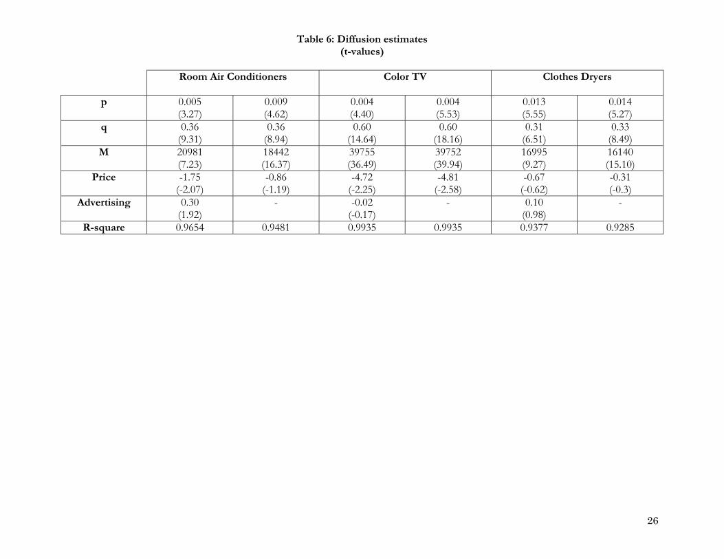
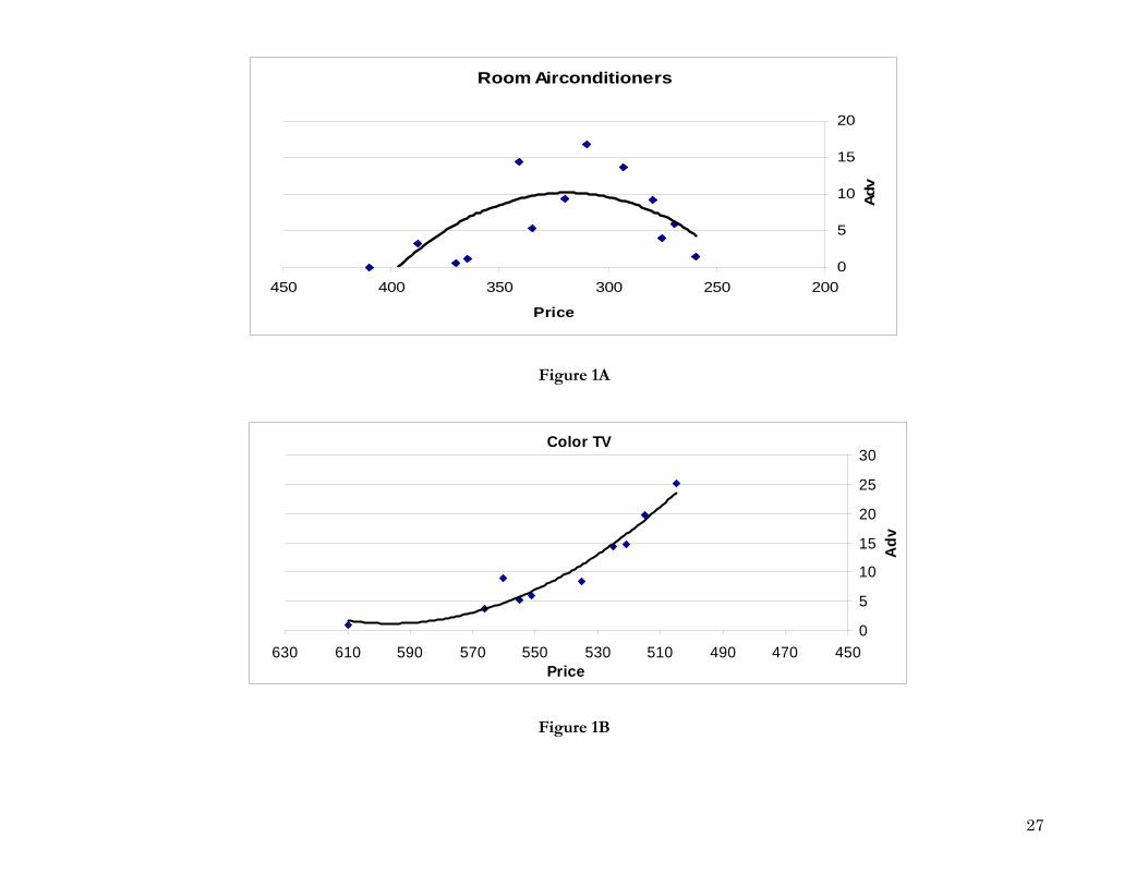
following example provides an illustration. Figure 1A shows the relationship between advertising

2

and prices over the room air conditioner life cycle. The superimposed trend line clearly suggests an

inverted-U relationship, and this is confirmed by the results of a regression model. Now, let us look

at Table 1 which contains the estimated parameters of the Generalized Bass Model (GBM - Bass,

Krishnan and Jain 1994) under two different scenarios: one in which only price is included as

marketing mix variable, and the other in which both price and advertising are included as marketing

mix variables. The results run seemingly counter to expectations! Price is not significant when it is

the sole marketing mix variable i.e. when advertising is not included in the model, but becomes

significant, along with advertising, when both are included! Thus, the inclusion of advertising in the

diffusion model leads to the “signification” of the pricing effect, a result not usually observed or

discussed in marketing literature. One in fact may have expected that due to multicollinearity i.e. the

relationship between advertising and pricing, the inclusion of both of the variables would lead to

“insignification” of one or both of them, but clearly what we see is an exact opposite effect.

The above illustration underlines the need to systematically examine the role of the price-advertising

relationship in the estimation of their impact on demand. Specifically, it suggests that when

information on one of the two marketing mix variables is not available, a plausible scenario, the

estimated effect of the included variable may be not only biased but also falsely insignificant. Said

differently, if a manager uses only the price data in his analysis of demand and finds the price

variable insignificant he cannot simply conclude that price is actually insignificant. This is because in

the absence of the advertising variable the estimate of price effect could be biased. The latent

relationship between price and advertising necessitates the inclusion of advertising variable also in

the demand estimation.

3

In this paper we formally explore through a series of simulations the role of price-advertising

relationship in the estimation of diffusion effects. We focus on the case where only the price variable

is included in the estimation while the missing advertising variable acts latently through its

relationship with price. We draw on econometric theory to design our simulations and form

expectations on the factors that influence bias, standard errors and significance of the estimates of

the included variable. We find that the strength (standard deviation of residual errors), direction

(positive/negative) and functional form (linear, quadratic, non-monotonic) of the pricing-advertising

relationship are all significant factors. We test, and verify, our findings using three data sets

previously used in diffusion literature.

The rest of the paper is organized as follows. The next section draws considerably on theory

regarding the price-advertising relationship and econometrics to provide a background for our study.

Section three describes the simulation method and the results. Section four provides an analysis of

the simulation results and an empirical application on three diffusion data sets. Section five

concludes with a summary, discussion of implications and avenues for future research.

2. Background Our background discussion is divided into two sections: the first is concerned with a literature

review on the price-advertising relationship and the second is related to econometric theory on the

consequences of omitting variables.

2.1 Price-advertising relationship

Views on the price-advertising relationship are opposing and corresponding empirical evidence

inconclusive (e.g. Vakratsas and Ambler 1999). This should be attributed to the complexity of the

relationship which is contingent upon a host of factors such as: content of advertising (price vs.

4

non-price, Kaul and Wittink 1995), price sensitivity of consumers (Albion and Farris 1980),

differentiation (Soberman 2004), manufacturer-retailer interaction (Steiner 1973) and market

expansion to name a few.

There are two major streams of thought on the price-advertising relationship: one associated with

the economics of information theory (Stigler 1961; Telser 1964) which suggests that advertising

should lead to lower prices since it facilitates information gathering and hence price-searching. The

other view is associated with the market power theory of advertising (Comanor and Wilson 1974)

which suggests that advertising in creating differentiation, leads to higher prices. The suggestion that

the advertising effect on prices is an indirect one, determined through its effect on price sensitivities

(e.g. Farris and Albion 1980), and that the manufacturer/retailer interaction is critical in determining

consumer prices (Steiner 1973) further complicates matters. In their empirical generalizations study,

Kaul and Wittink (1995) attempted to reconcile the two views by suggesting that price advertising

will reduce prices whereas non-price advertising will decrease price sensitivities (and possible

increase prices as per Farris and Albion 1980). However, recently Soberman’s theoretical study

suggested that prices may increase even when advertising is informative, depending the level of

differentiation (high vs. low).

The brief summary of relevant studies indicates that the price-advertising relationship is

idiosyncratic, depending on various market conditions, which could explain the lack of consistent

empirical evidence. This implies that an investigation on the effects of the price-advertising

relationship on demand should take into account different directions of the relationship

(positive/negative). Furthermore, no study, to our knowledge, has examined the functional form of

such a relationship. Yet, Montgomery and Bradlow (1999) found that the choice of functional form

5

is critical for the estimation of the pricing effect on demand. Based on these conclusions, we intend

to account for both direction and shape of the price-advertising relationship.

2.2 Econometric Theory on Omitted Variables

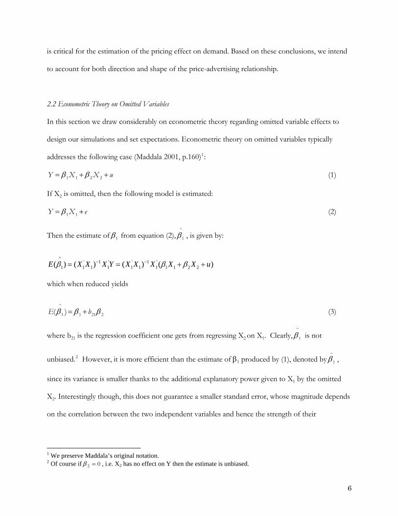
In this section we draw considerably on econometric theory regarding omitted variable effects to

design our simulations and set expectations. Econometric theory on omitted variables typically

addresses the following case (Maddala 2001, p.160)1:

uXXY ++= 2211 ββ (1)

If X2 is omitted, then the following model is estimated:

eXY += 11β (2)

Then the estimate of 1β from equation (2), , is given by: ^

1β

^' 1 ' ' 1 '

1 1 1 1 1 1 1 1 1 2 2( ) ( ) ( ) ( )E X X X Y X X X X X uβ β− −= = + β +

which when reduced yields

2211

^

1 )( βββ bE += (3)

where b21 is the regression coefficient one gets from regressing X2 on X1. Clearly, is not

unbiased.

^

1β

2 However, it is more efficient than the estimate of β1 produced by (1), denoted by ,

since its variance is smaller thanks to the additional explanatory power given to X1 by the omitted

X2. Interestingly though, this does not guarantee a smaller standard error, whose magnitude depends

on the correlation between the two independent variables and hence the strength of their

~

1β

1 We preserve Maddala’s original notation. 2 Of course if 02 =β , i.e. X2 has no effect on Y then the estimate is unbiased.

6

relationship. See equation 4 below which gives the variance of the estimate as a function of the

variance of the estimate .

^

1β

~

1β

12

2.1

⎛ ⎞

⎝ ⎠

2^ ~2 2

1 1 2

1( ) ( )

1y

rS S

rβ β

−⎜ ⎟=⎜ ⎟−

, (4)

where is the correlation between the two explanatory variables X1 and X2, and is the

partial correlation between Y and X2.

212r 2

1.2yr

Thus, there are two levels of bias we encounter when we omit a variable that has a latent

relationship with the included variable. One bias is associated with the mean of the estimate of the

included variable, and the other with the estimate of its variance. However, besides these broad

statistical guidelines, standard econometric theory does not offer any further insights with regards to

the magnitude and the direction of bias, and with respect to the magnitudes of the standard errors.

Noting that the significance of an estimate depends on both its absolute value and the standard

error3, this can lead to a host of different scenarios in terms of the significance of the included

variable effect. For example, a marginally biased estimate may be tested insignificant due to a high

standard error if the relationship between the two variables is not strong (low correlation). On the

other hand, a highly biased estimate could be tested significant if the relationship between the two

variables is strong (low standard error). Perhaps more importantly for marketing, the direction of the

relationship between the two explanatory variables as well as their effects on the dependent variable,

can influence the extent (and direction) of the bias and, consequently, the statistical significance of

3 The t-statistic is given by “(estimate - true value)/standard error”.

7

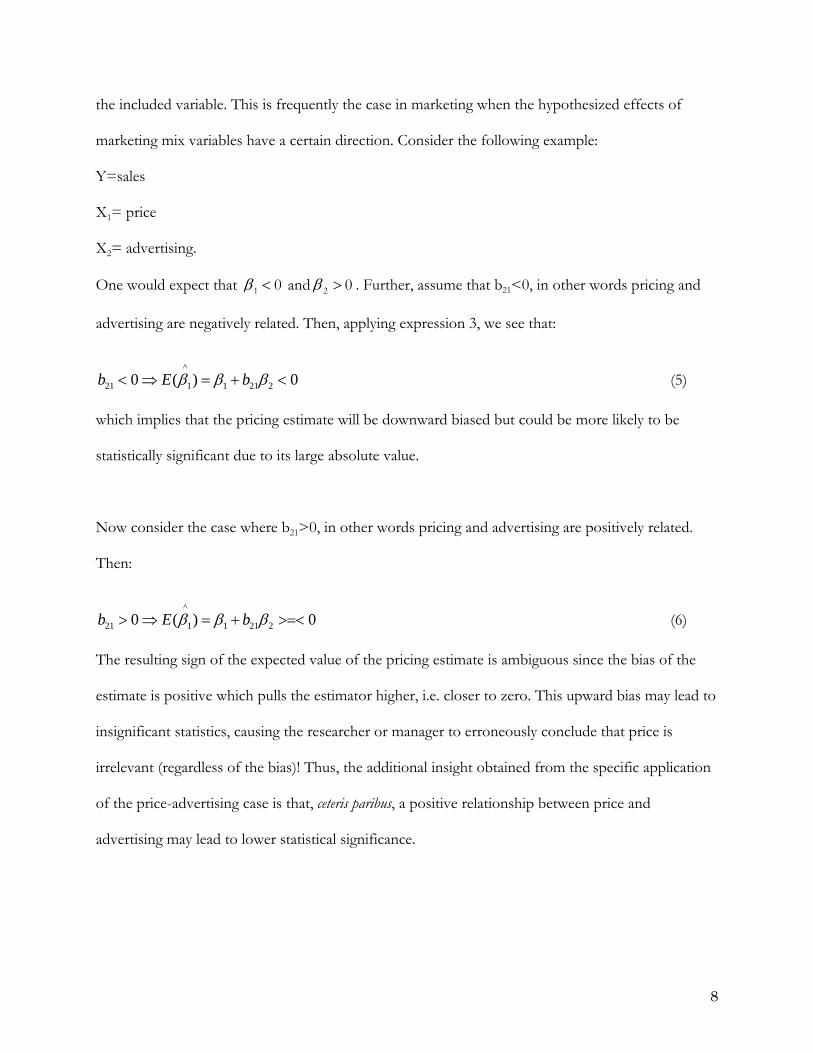
the included variable. This is frequently the case in marketing when the hypothesized effects of

marketing mix variables have a certain direction. Consider the following example:

Y=sales

X1= price

X2= advertising.

One would expect that 01 <β and 02 >β . Further, assume that b21<0, in other words pricing and

advertising are negatively related. Then, applying expression 3, we see that:

^

21 1 1 21 20 ( )b E bβ β β< ⇒ = + < 0

0

(5)

which implies that the pricing estimate will be downward biased but could be more likely to be

statistically significant due to its large absolute value.

Now consider the case where b21>0, in other words pricing and advertising are positively related.

Then:

^

21 1 1 21 20 ( )b E bβ β β> ⇒ = + >=< (6)

The resulting sign of the expected value of the pricing estimate is ambiguous since the bias of the

estimate is positive which pulls the estimator higher, i.e. closer to zero. This upward bias may lead to

insignificant statistics, causing the researcher or manager to erroneously conclude that price is

irrelevant (regardless of the bias)! Thus, the additional insight obtained from the specific application

of the price-advertising case is that, ceteris paribus, a positive relationship between price and

advertising may lead to lower statistical significance.

8

Since in our application we plan to use advertising as the omitted variable, just as in the previously

discussed stylized example, the following two broad implications may be drawn from standard

econometric theory on linear models and our stylized observations on the price-advertising case:

-The stronger the relationship between price and advertising, the lower the standard error of the price estimate

-A positive relationship between price and advertising will cause upward bias, leading to higher likelihood of

insignificant price estimates than in the case of a negative relationship.

The above expectations are of course based on theory and observations concerning the linear case.

However, in the case of diffusion the demand model is nonlinear and it is likely that the price-

advertising relationship is also nonlinear if not non-monotonic. Furthermore, statistics in the non-

linear case are asymptotic rather than exact. Hence these expectations are tentative and should be

only used as guidelines for setting up the simulations which should provide a definitive answer.

Next, we discuss the simulation method in detail and outline the alternative scenarios.

3. Simulation method and scenarios

Based on our review of econometric theory, we expect that if we omit advertising and include only

price in the demand model estimation then the price estimate will be affected by (1) the strength of

the latent relationship between price and advertising and (2) the direction of that latent relationship.

We measure the impact on price estimate through looking at its bias, standard error and eventual

statistical significance. Why did we choose to omit advertising and include price instead of keeping

price variable as omitted and include advertising? We do so because this is what many managers face

in the real world, and what many of them would be interested in. Secondly, as a researcher, it is

9

practically easier to observe pricing rather than advertising. Thirdly, advertising is more likely to be

endogenous and driven by pricing rather than the other way around, since cost is a major driver of

prices especially for durable goods (e.g. Bass 1980). However, the essence of our findings is

preserved if the price-advertising role is reversed.

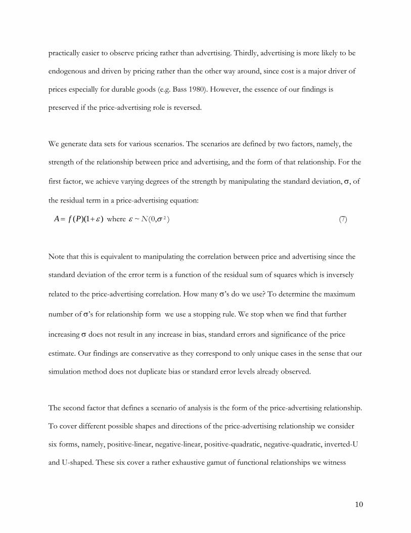
We generate data sets for various scenarios. The scenarios are defined by two factors, namely, the

strength of the relationship between price and advertising, and the form of that relationship. For the

first factor, we achieve varying degrees of the strength by manipulating the standard deviation, σ, of

the residual term in a price-advertising equation:

( )(1 )A f P ε= + where ),0(~ 2σε N (7)

Note that this is equivalent to manipulating the correlation between price and advertising since the

standard deviation of the error term is a function of the residual sum of squares which is inversely

related to the price-advertising correlation. How many σ’s do we use? To determine the maximum

number of σ’s for relationship form we use a stopping rule. We stop when we find that further

increasing σ does not result in any increase in bias, standard errors and significance of the price

estimate. Our findings are conservative as they correspond to only unique cases in the sense that our

simulation method does not duplicate bias or standard error levels already observed.

The second factor that defines a scenario of analysis is the form of the price-advertising relationship.

To cover different possible shapes and directions of the price-advertising relationship we consider

six forms, namely, positive-linear, negative-linear, positive-quadratic, negative-quadratic, inverted-U

and U-shaped. These six cover a rather exhaustive gamut of functional relationships we witness

10

typically in a new product sales growth. For example, for some goods prices and advertising may

both initially be declining due to experience curve effects (for pricing) and high introductory

advising expenditure (for advertising). Later on, however, advertising may increase while prices are

still declining in an effort to broaden the appeal of the product and expand the market. For other

products, low prices may be systematically supported throughout the life-cycle by higher advertising,

implying a negative monotonic relationship. For ease of exposition, the simulation conditions are

summarized in Table 2, which also includes the pricing equation used to generate the pricing data

that captures experience curve effects, as well as the diffusion equation used to generate the sales

data. We kept the standard deviation of prices, υ, at a low value (0.05) in order to have a minimal

influence on our results. Some variation, however, was necessary to construct a realistic data-

generating process for prices.

Thus we have six forms of relationship and multiple σ i.e. degrees of strength-of-relationship. Each

form-σ combination pertains to a scenario. We ended up with 44 scenarios. For each of the 44

scenarios, we simulated the results 100 times using different starting random numbers for the error

terms in the data generation process and then took the mean and standard error of the resulting

distribution of the mean of the price coefficient estimate. The time horizon in each scenario or

simulation run is set at 40 periods because the sales growth curve peaks and comes down to almost

zero sales within 40 periods.

Table 3 summarizes the main findings regarding mean estimated price coefficient, its standard error

and mean bias (in real terms). We also evaluated for each scenario how many of the 100 simulation

runs produced significant price coefficient estimate, and this statistic is given by the “Significant

11

cases” in Table 3. The summary statistics are also illustrated in a series of figures (Figure 2),

corresponding to each functional form.

There are some clear trends emerging from the Table and Figures:

1. Standard errors are systematically increasing with σ. This is consistent with our expectation

that a stronger price-advertising relationship should lead to lower errors of the estimate.

2. For positive price-advertising relationships the bias is upwards (and in fact positive!),

whereas for negative relationships it is downwards. This is in line with what we proposed.

3. Looking at the graphs we see that the bias generally but systematically declines in terms of

real values (i.e. becomes smaller) when σ increases. This implies absolute bias increases in

the negative case but decreases in the positive case. Hence there appears to be a systematic

relationship between the strength of the price-advertising relationship and bias conditional

on the direction of the price-advertising relationship.

4. The number of significant cases (out of a maximum of 100) decreases sharply with σ in all of

the six forms of relationship, but such a drop is significantly more dramatic for positive

forms of relationship, as per expectations, and also for non-monotonic relationships of price

and advertising.

A more formal validation of these observations based on a statistical analysis of the findings follows

in the next section, which also contains empirical tests using actual diffusion data.

4. Empirical analysis

We divide this section into two parts, one concerning the analysis of the simulation results reported

in Table 3 and the second discussing the empirical analysis of the three diffusion data sets.

12

4.1 Analysis of simulation results

We formalize our observations of the previous section by statistically testing the determinants of

bias, standard errors, and significance of the pricing effect when advertising is omitted. We

distinguish among three major factors: (a) strength of price-advertising relationship (σ), (b) direction

of price-advertising relationship (positive/negative) and (c) functional form of relationship (linear,

quadratic, non-monotonic).

The equations have the following general form:

iiiiiii positiveicnonmonotonlineary νααασαα +++++= 43210 (8)

where:

i=1,2,3 and:

1y =mean absolute bias, =mean standard error and =significant cases (out of a maximum 100) 2y 3y

linear =1 if functional form is linear and 0 otherwise,

nonmonotonic =1 if functional form is non-monotonic and 0 otherwise

positive =1 if the direction of relationship is positive and 0 otherwise (including the non-monotonic

cases)

iv are the usual normal error terms.

Hence the negative and quadratic cases are the baselines in our regression. We also ran an additional

regression for mean absolute bias with an interaction between σ and positive to check whether a

weakening relationship between price and advertising moderates the effect of a positive relationship

on bias, as remarked earlier.

13

A summary of results is provided in Table 4. The fit of all three equations with main effects is good

with very high R-squares, providing an implicit validation for our choice of determining factors. The

findings thoroughly confirm our expectations and validate our observations:

1. The strength of price-advertising relationship has a significant positive effect on standard

errors and a negative effect on significance. Thus, a weak relationship between price and

advertising leads to higher standard errors for the price coefficient as expected from

econometric theory based on the study of linear models. Somewhat less expectedly, σ is also

strongly related to absolute bias and has a significant positive effect. Thus, we managed to

establish a link between price-advertising relationship strength and bias that was not been

previously discussed in the literature. The two effects taken together suggest that a weak

price-advertising relationship may lead either to a non-significant effect (significance

equation) or a strongly biased estimate of the price coefficient.

2. The direction and functional form of the relationship are also significant with the exception

of the standard error equation, which is dominated by the effects of the strength of the

relationship between price and advertising. One possible explanation for the lack of

significance of the functional form in the standard error equation is that we stop the

simulations at a level of σ beyond which standard errors plateau, hence we include a

different number of levels of σ for each functional form that correspond to unique standard

errors. Thus the results suggest that for levels of σ included in the simulations, standard

errors do not depend on functional form. If we were to include “duplicate” cases producing

similar standard errors for different levels of σ then we could have obtained significant

results but we opted for the more stringent case of unique observations.

14

3. A quadratic functional form produces the most bias and a linear the least. A quadratic

relationship, however, produces the most significant cases likely due to the high bias. In

some cases such a bias produces even (erroneous) positive price coefficients as observed in

Table 3. Thus, when price and advertising are related in a quadratic fashion the findings on

the pricing effect should be qualified with caution. A non-monotonic relationship produces

the least number of significant cases despite the relatively low bias, suggesting that these

cases are particularly vulnerable to standard errors.

4. Similarly to the non-monotonic case, a positive relationship (applicable only to monotonic

functional forms) produces smaller bias but also fewer significant cases. This is consistent

with our second expectation, based on linear models, that a positive relationship will

produce more insignificant cases. Due to the negative expected sign of the pricing

coefficient, a positive relationship causes an upward bias which results in a smaller absolute

value. Consequently, the inference would misleadingly point to an insignificant relationship.

The significant effects of functional form on significance implicitly, but clearly, suggest that

bias plays an important role on significance inference and even significant price coefficients

may be the result of heavy bias.

To our knowledge, this is a unique contribution of our study since we managed to formalize the

relationship between direction of the relationship (positive/negative), estimate bias and, ultimately,

statistical significance. We also find that indeed the absolute bias is smaller when the relationship

between pricing and advertising is positive and weakening (higher σ). Thus it appears that when the

two variables become more independent, the bias is smaller when they move in the same (positive

relationship) rather than opposite (negative relationship) directions.

15

4.2 Empirical analysis of diffusion data sets

We test our findings on three diffusion datasets previously analyzed by Bass, Krishnan and Jain

(1994). To our knowledge, these are the only diffusion data sets that include both pricing and

advertising information. First, we investigate the price-advertising relationship to identify the

simulation case which is closer to the reality. To accommodate various directions and functional

forms we use the following quadratic relationship:

tttt ePPcA +++= 221 λλ (9)

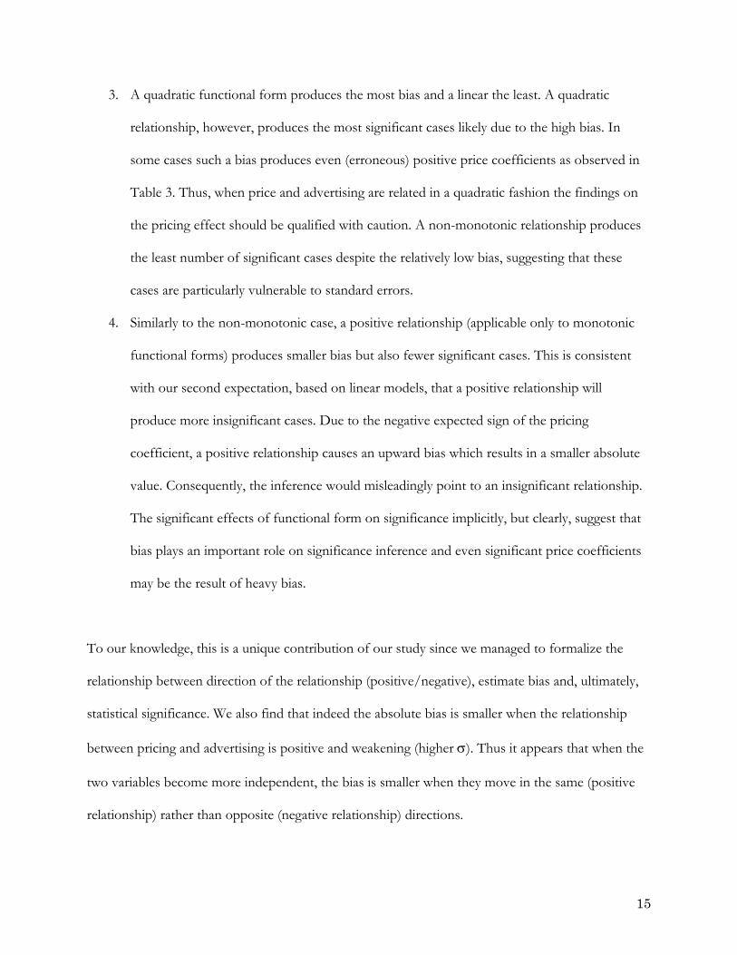
The results for the three categories are summarized in Table 5. For Room Air-conditioners the

relationship between price and advertising is inverted-U shaped and is moderately strong; for

clothes-dryers the relationship has similar form but is rather weak; for Color TV the relationship is

non-linear monotonic and very strong. See also Figures 1A and 1B. Thus, according to our

simulation results, it appears that the room air-conditioner case with a non-monotonic but not

particularly strong relationship between price and advertising could be susceptible to producing non-

significant pricing estimates due to high standard errors. The strong relationship in the Color TV

case, on the other hand, should produce low standard errors but may lad to bias affecting the

significance of the pricing estimate. Finally the lack of significant estimates in the clothes-dryers

equation suggests independence of pricing and advertising and hence omission of the latter should

not affect estimates of the former. Hence, the air-conditioner case appears to be the most interesting

and relevant to our study.

We now turn to the estimation of diffusion effects for the three data sets. We use the same

estimation method (Generalized Bass Model) as in the original reference hence we omit details for

brevity reasons. Table 6 contains the estimation results when both variables and only price are

16

included in the model. The findings for room-air conditioners confirm our expectations: when only

price is included its effect is insignificant but the inclusion of advertising seems to correct the pricing

significance as well. While there is a clear inverted-U relationship between prices and advertising it is

moderately strong, affecting thus the significance of the price estimate. The cases of Color TVs and

clothes dryers are different. The price coefficient is significant in the price-only model and changes

very little when advertising is included in the case of color TVs. While this could be due to the high

strength of the price-advertising relationship (producing low standard errors) it should also be

attributed to the insignificance of the advertising effect. From an informational perspective, the

addition of advertising in the model does not contribute to further explanation of the variability and

hence its omission does not have an effect on the price estimate as it is irrelevant to the diffusion

(the equivalent of 2β being zero in the linear case of equation 3). For clothes dryers, none of the

two variables significantly affects the diffusion process hence the omission of advertising is not

expected to have significant consequences on the price coefficient estimate. Furthermore, price and

advertising are independent in this case hence omission of one should not affect the estimate of the

other. In line with this expectation, the t-value of the price coefficient estimate increases in absolute

value when adv is also included (it goes from -0.3 to -0.6) but the increase is not strong enough to

make the price effect significant as in the Room Air-conditioners case.

5. Implications, Conclusion and Future Research

Whereas the effect of pricing and advertising on demand has probably been one of the most

extensively researched areas in marketing, the role of the relationship between these two marketing

mix variables on the estimation of market outcomes has been largely overlooked. A potential reason

for such a dearth of research in this area is the complexity of the relationship between pricing and

advertising, which could lead to a variety of scenarios that would be difficult to examine. In this

17

study we precisely undertake such an initiative by investigating the role of the price-advertising

relationship in the context of diffusion of innovations. An added complexity of diffusion –style

demand models is that they are non-linear, hence the effects of the price-advertising relationship is

difficult to uncover. We address this issue by conducting simulations that control the functional

form of the relationship between price and advertising, the strength of such relationship (in the form

of the standard deviations of residual errors in the price-advertising equation), and the direction of

the relationship (positive/negative). Nevertheless, we draw upon econometric theory on linear

models to form corresponding and testable expectations.

Our simulation results suggest that all three factors have a significant effect on mean absolute bias of

the pricing coefficient when advertising is not included in the diffusion equation. Quadratic

relationships produce the highest bias and a positive quadratic relationship produces even

(erroneous) positive pricing estimates, some of them being significant! As for estimated price

coefficient standard errors, the major driver is the strength of the relationship between pricing and

advertising: the weaker such a relationship, the larger the standard error. All these effects naturally

influence the significance of the price coefficient. The significant effects of the functional form and

the direction of the relationship on the volume of significant cases imply that not only the standard

error, but also the bias determines the significance of the pricing coefficient. This is obvious in the

quadratic cases, which tend to produce the highest significance incidence. However, such

significance is misleading since it appears to be the result of high bias which even produces price

coefficients with wrong (positive) signs. Hence, researchers and managers should be cautious when

they try to estimate pricing effects on diffusion in the absence of the advertising variable. This can

be a very common case since pricing information is much easier to obtain through direct

observation rather than advertising.

18

Our findings are also consistent with econometric theory expectations, drawn from the study of

linear models, that a weaker relationship between pricing and advertising will produce higher

standard errors. A novel finding of our study, and a contribution in addition to the study of complex

relationships and non-linear demand models, is the effect of the direction of the relationship on the

bias of the pricing estimate and , consequently, on its significance. Specifically, we found that a

positive price-advertising relationship leads to a smaller absolute bias. This should be interpreted as

an “upward” bias since the expected sign of the pricing effect is negative. As a result, when the

relationship is positive the number of significant cases, misleadingly, reduces.

A fruitful area of future research would be the correction of the pricing effect in the absence of

advertising information. This can be accomplished by using a variable that is not correlated with

pricing or time (which is an underlying force of the diffusion phenomenon) but mimics the

advertising pattern over time.

19

20

References

Bass, Frank M. (1980), “The Relationship between Diffusion Rates, Experience Curves and Demand

Elasticities for Consumer Durable Technological Innovations,” Journal of Business, 53(3), S51-

S67.

Bass, Frank M., Trichy Krishnan and Dipak C. Jain (1994), “Why the Bass Model Fits Without

Decision Variables,” Marketing Science, 13(3), 203-223.

Comanor, William S. and Thomas A. Wilson (1974), Advertising and Market Power, Cambridge, MA:

Harvard University Press.

Farris, Paul W. and Mark S. Albion (1980), “The Impact of Advertising on the Price of consumer

Products,” Journal of Marketing, 44 (Summer), 17-35.

Kaul, Anil and Dick R. Wittink (1995), “Empirical Generalizations About the Impact of Advertising

on Price Sensitivity and Price,” Marketing Science, 14(3, part 2), G151-G160.

Maddala, G.S. (2001), An Introduction to Econometrics, 3rd ed., New York: John Wiley and Sons.

Montgomery, Alan L. and Eric T. Bradlow (199), “Why Analyst Overconfidence About the

Functional Form of Demand May Lead to Overpricing,” Marketing Science, 18(4), 569-583.

Soberman, David A. (2004), “Research Note: Additional Learning and Implications on the Role of

Informative Advertising,” Management Science, 50(12), 1744-1750.

Steiner, Robert (1973), “Does Advertising Lower Consumer Prices?” Journal of Marketing, 37, 19-26.

Stigler, George (1961) “The Economics of Information,” Journal of Political Economy,

69(January/February), 213-225.

Telser, Lester G. (1964), “Advertising and Competition,” Journal of political Economy, 72(December),

537-562.

Vakratsas, Demetrios and Tim Ambler (1999), “How Advertising Works: What Do We Really

Know?” Journal of Marketing, 63(1), 26-43.

Table 1: GBM results for Room Air-conditioners (t-values)

p 0.005 (3.27)

0.009 (4.62)

q 0.36 (9.31)

0.36 (8.94)

M 20981 (7.23)

18442 (16.37)

Price -1.75 (-2.07)

-0.86 (-1.19)

Advertising 0.30 (1.92)

-

21

Table 2: Summary of Simulation Conditions*

Price-Advertising

Relationship Advertising Equation Price

Equation Diffusion Equation

1 Negative Linear

)1)(5.0300( ε+−= PA

2 Positive Linear

)1)(5.0100( ε++= PA

3 Negative Quadratic

)1)(001.04.010( 2 ε+−+= PPA

4 Positive Quadratic

)1)(001.04.050( 2 ε++−= PPA

5 Inverted-U

)1)(001.065.050( 2 ε+−+−= PPA

6 U-Shaped

)1)(001.065.0150( 2 ε++−= PPA

)1(400 01.0 υ+= − teP)05.0,0(~ Nυ

1( )(1 ),t t t sS M F F whereε−= − +

(0,0.01)s Nε = , 1 exp( ( ) )

1 *exp( ( ) ) / ,t

t

c d ht d c d h cF where− − +

+ − +=

0 0

PPln ln ,t tA

t pr ad Ah t whereβ β= + +

P=Price, A=advertising c, d are Bass model parameters

M is market size

*Note that we used both price and advertising in generating the sales data but used only price in the estimation.

22

23

Table 3: Summary of Simulation Results (Advertising variable is omitted): 44 Scenarios*

P-A error standard deviation (σ) Price-Advertising Relationship 0.01 0.05 0.1 0.2 0.25 0.4 0.5 0.6 0.7

1 Negative Linear Price coefficient Standard error Bias Significant cases

Scenario1 -2.13 0.09 -1.13 100

Scenario2 -2.15 0.25 -1.15 96

Scenario3 -2.17 0.48 -1.17 47

Scenario4 -2.23 0.99 -1.23

9

Scenario5 -2.25 1.30 -1.25

6

Scenario6 -2.34 2.81 -1.34

2

Scenario7 -2.45 4.09 -1.45

2

Scenario8 -2.96 4.93 -1.96

4

Scenario9 -2.37 9.99 -1.37

8 2 Positive Linear

Price coefficient Standard error Bias Significant cases

Scenario10 -0.5 0.05 0.5 76

Scenario11 -0.52 0.23 0.48

0

Scenario12 -0.55 0.46 0.45

0

Scenario13 -0.59 0.96 0.41

0

Scenario14 -0.61 1.26 0.39

0

3 Negative Quadratic Price coefficient Standard error Bias Significant cases

Scenario15 -4.64 0.86 -3.64 96

Scenario16 -4.66 0.90 -3.66 94

Scenario17 -4.69 1.02 -3.69 91

Scenario18 -4.74 1.39 -3.74 80

Scenario19 -4.77 1.64 -3.77 68

Scenario20 -4.93 2.95 -3.93 35

Scenario21 -4.91 4.29 -3.91 28

Scenario22-5.40 4.79 -4.40 28

Scenario23 -5.55 9.21 -4.55 19

4 Positive Quadratic Price coefficient Standard error Bias Significant cases

Scenario241.55 0.06 2.55 100

Scenario25 1.53 0.22 2.53 94

Scenario26 1.50 0.44 2.50 27

Scenario27 1.46 0.94 2.46

3

Scenario28 1.45 1.23 2.45

2

Scenario291.55 3.97 2.55

1

Scenario301.42 3.86 2.42

1

5 Inverted-U Price coefficient Standard error Bias Significant cases

Scenario31-1.25 0.11 -0.25 82

Scenario32 -1.27 0.25 -0.27

5

Scenario33 -1.29 0.48 -0.29

0

Scenario34 -1.34 0.99 -0.34

0

Scenario35 -1.36 1.29 -0.36

0

Scenario36-1.24 3.75 -0.24

0

Scenario37-1.53 4.02 -0.53

1

6 U-Shaped Price coefficient Standard error Bias Significant cases

Scenario38-0.74 0.11 0.26

7

Scenario39 -0.76 0.24 0.24

0

Scenario40 -0.79 0.46 0.21

0

Scenario41 -0.84 0.96 0.16

0

Scenario42 -0.86 1.26 0.14

0

Scenario43-0.73 3.75 0.27

0

Scenario44-1.02 3.99 -0.02

0

*The statistics (coefficient, standard error, and bias) mentioned in each scenario are the means of 100 simulation runs. The “Significant cases” entry counts the number of times (out of 100 maximum runs) the estimation resulted in a significant price coefficient estimate.

24

Table 4: Analysis of Simulation Results (t-values)

Mean

Absolute Bias Mean Standard

error Significant

Cases Intercept 3.64

(44.56) 3.60

(48.00) -0.17

(-0.49) 96.34

(10.27) P-A relationship strength

(σ) 0.52

(3.25) 0.72

(4.53) 10.02

(14.88) -117.68 (-6.35)

Linear -2.35 (-30.82)

-2.39 (-34.12)

-0.14 (-0.45)

-29.30 (-3.34)

Non-monotonic -3.50 (-41.11)

-3.50 (-45.51)

-0.45 (-1.25)

-64.17 (-6.57)

Positive -1.12 (-13.83)

-0.87 (-8.11)

-0.40 (-1.20)

-38.00 (-4.10)

σ x positive - -1.26 (-3.13)

- -

R-square 0.98 0.98 0.87 0.64 Adjusted R-square 0.98 0.98 0.86 0.60

25

Table 5: Price-advertising equation estimates (t-values)

Room Air Conditioners Color TV Clothes Dryers

Intercept -158.8 (-2.29)

956.7 (4.66)

-172.6 (-1.27)

Price 1.06 (2.49)

-3.20 (-4.33)

1.64 (1.30)

Price2 -0.002 (-2.59)

0.003 (4.04)

-0.004 (-1.31)

R-square 0.47 0.94 0.15

26

Table 6: Diffusion estimates (t-values)

Room Air Conditioners Color TV Clothes Dryers

p 0.005 (3.27)

0.009 (4.62)

0.004 (4.40)

0.004 (5.53)

0.013 (5.55)

0.014 (5.27)

q 0.36 (9.31)

0.36 (8.94)

0.60 (14.64)

0.60 (18.16)

0.31 (6.51)

0.33 (8.49)

M 20981 (7.23)

18442 (16.37)

39755 (36.49)

39752 (39.94)

16995 (9.27)

16140 (15.10)

Price -1.75 (-2.07)

-0.86 (-1.19)

-4.72 (-2.25)

-4.81 (-2.58)

-0.67 (-0.62)

-0.31 (-0.3)

Advertising 0.30 (1.92)

- -0.02 (-0.17)

- 0.10 (0.98)

-

R-square 0.9654 0.9481 0.9935 0.9935 0.9377 0.9285

Room Airconditioners

0

5

10

15

20

200250300350400450

Price

Adv

Figure 1A

Color TV

0

5

10

15

20

25

30

450470490510530550570590610630Price

Adv

Figure 1B

27

28

Figure 2

Negative Linear

-4

-2

0 2 4 6 8

10 12

0.01 0.05 0.1 0.2 0.25 0.4 0.5 0.6 0.7

mean standard error

mean bias

Significant cases(scaled)

Positive Linear

0

0.2

0.4

0.6

0.8

1

1.2

1.4

0.01 0.05 0.1 0.2 0.25

mean standard error

mean bias

Significant cases(scaled)

Negative Quadratic

-6

-4

-2

0 2 4 6 8

10

0.01 0.05 0.1 0.2 0.25 0.4 0.5 0.6 0.7

mean standard error

mean bias

Significant cases(scaled)

Positive Quadratic

0

0.5

1

1.5

2

2.5

3

3.5

4

4.5

0.01 0.05 0.1 0.2 0.25 0.4 0.5

mean standard error

mean bias

Significant cases(scaled)

Inverted-U

-1

0

1

2

3

4

5

0.01 0.05 0.1 0.2 0.25 0.4 0.5

mean standard error

mean bias

Significant cases(scaled) Significant cases(scaled)

mean standard error

mean bias

0.5

U-shaped

0.40.250.20.1 0.050.01

4

3

2

1

0

-0.5

4.5

3.5

2.5

1.5

0.5