PRESSURE-DEPENDENT EPANET EXTENSION · PDF file2 PRESSURE-DEPENDENT EPANET EXTENSION Calvin...
33
1 PRESSURE-DEPENDENT EPANET EXTENSION Calvin Siew 1 and Tiku T. Tanyimboh 2 Department of Civil Engineering, University of Strathclyde Glasgow. John Anderson Building, 107 Rottenrow, Glasgow G4 0NG, UK. 1 PhD student, Department of Civil Engineering, University of Strathclyde Glasgow. John Anderson Building, 107 Rottenrow Glasgow G4 0NG, UK. Email : [email protected] Tel : +44 (0) 141 548 3578 2 Corresponding Author. Senior Lecturer, Department of Civil Engineering, University of Strathclyde Glasgow. John Anderson Building, 107 Rottenrow Glasgow G4 0NG, UK. Email : [email protected] Tel : +44 (0)141 548 4366 FAX : +44 (0)141 553 2066 This article was published in Water Resources Management (2012) 26:1477–1498. Water Resources Management April 2012, Volume 26, Issue 6, pp 1477-1498 Pressure-Dependent EPANET Extension Calvin Siew, Tiku T. Tanyimboh The final publication is available at http://link.springer.com/article/10.1007/s11269- 011-9968-x.springer.com.
Transcript of PRESSURE-DEPENDENT EPANET EXTENSION · PDF file2 PRESSURE-DEPENDENT EPANET EXTENSION Calvin...
1
PRESSURE-DEPENDENT EPANET EXTENSION
Calvin Siew1 and Tiku T. Tanyimboh
2
Department of Civil Engineering, University of Strathclyde Glasgow.
John Anderson Building, 107 Rottenrow, Glasgow G4 0NG, UK.
1
PhD student, Department of Civil Engineering, University of Strathclyde Glasgow.
John Anderson Building, 107 Rottenrow Glasgow G4 0NG, UK.
Email : [email protected]
Tel : +44 (0) 141 548 3578
2
Corresponding Author.
Senior Lecturer, Department of Civil Engineering, University of Strathclyde Glasgow.
John Anderson Building, 107 Rottenrow Glasgow G4 0NG, UK.
Email : [email protected]
Tel : +44 (0)141 548 4366
FAX : +44 (0)141 553 2066
This article was published in Water Resources Management (2012) 26:1477–1498.
Water Resources Management
April 2012, Volume 26, Issue 6, pp 1477-1498
Pressure-Dependent EPANET Extension
Calvin Siew, Tiku T. Tanyimboh
The final publication is available at http://link.springer.com/article/10.1007/s11269-
011-9968-x.springer.com.
2
PRESSURE-DEPENDENT EPANET EXTENSION
Calvin Siew and Tiku T. Tanyimboh
Department of Civil Engineering, University of Strathclyde Glasgow, UK
Abstract
In water distribution systems (WDSs), the available flow at a demand node is
dependent on the pressure at that node. When a network is lacking in pressure, not all
consumer demands will be met in full. In this context, the assumption that all
demands are fully satisfied regardless of the pressure in the system becomes
unreasonable and represents the main limitation of the conventional demand driven
analysis (DDA) approach to WDS modelling. A realistic depiction of the network
performance can only be attained by considering demands to be pressure dependent.
This paper presents an extension of the renowned DDA based hydraulic simulator
EPANET 2 to incorporate pressure-dependent demands. This extension is termed
“EPANET-PDX” (pressure-dependent extension) herein. The utilization of a
continuous nodal pressure-flow function coupled with a line search and backtracking
procedure greatly enhance the algorithm’s convergence rate and robustness.
Simulations of real life networks consisting of multiple sources, pipes, valves and
pumps were successfully executed and results are presented herein. Excellent
modelling performance was achieved for analysing both normal and pressure deficient
conditions of the WDSs. Detailed computational efficiency results of EPANET-PDX
with reference to EPANET 2 are included as well.
Keywords Demand-driven analysis • Head-dependent modelling • Head-flow
relationship • Pressure-dependent demand • Pressure-deficient water distribution
system
3
1 Introduction
Pressure deficient conditions are inevitable in water distribution systems (WDSs) and
can be caused by common occurrences such as pump failure, pipe bursts, isolation of
major pipes from the system for planned maintenance work (Park et al. 2010,
Christodoulou 2010) and excessive fire fighting demands. Under these circumstances,
the WDS may not be able to satisfy all consumer demands. This requires water
companies to accurately model and analyse the WDS for crucial decision making.
However, the widely used demand driven analysis (DDA) is inappropriate for
modelling pressure deficient networks. This conventional model is formulated under
the assumption that demands are fully satisfied regardless of the pressure and yields
lower or even negative nodal pressure while analysing a pressure deficient network.
Hence, DDA is unable to accurately quantify the exact magnitude of deficiency in
terms of nodal pressure and outflow. This is critical information that cannot be
overlooked during a WDS performance evaluation. The need for an analysis
methodology that explicitly takes into account the relationship between nodal flows
and pressure cannot be further stressed. This method is known as pressure dependent
analysis (PDA) and models the WDS in a more realistic manner (Tabesh et al. 2009,
Martinez-Rodriguez et al. 2011).
There are numerous methods of obtaining the available nodal flow for PDA in the
literature. These methods can generally be categorized into two. The first category
comprises of methods involving demand driven analysis. For example, Ang and
Jowitt (2006) proposed an algorithm which progressively adds artificial reservoirs to
pressure deficient nodes. The approach used is similar to that of Bhave (1991).
Rossman (2007) implemented pressure dependent demands by modelling emitters as
orifices at nodes. Kalungi and Tanyimboh (2003) developed a heuristic in which some
aspects of PDA were used in a DDA environment to identify zero and partial flow
nodes. Gupta and Bhave (1996) developed an iterative approach which adjusted nodal
flows using several DDA runs. Aside from Rossman (2007), all of the methods
mentioned involve repetitive use of DDA with successive adjustments made to
specific parameters until a sufficient hydraulic consistency is obtained. This can lead
to high computational requirement and may present difficulties to be effectively
implemented for large networks.
The second category involves the approach where a head-flow relationship (HFR) is
embedded in the system of hydraulic equations. HFRs are functions used to estimate
the actual flow at demand nodes based on the nodal pressure. HFRs available in the
literature include Tanyimboh and Templeman (2004, 2010), Udo and Ozawa (2001),
Germanopoulos (1985), Gupta and Bhave (1996), Fujiwara and Ganesharajah (1993),
Cullinane et al. (1992) and Wagner et al. (1988). In general, these formulae have been
defined on the basis that nodal demand is satisfied in full when the nodal head is equal
to or greater than the desired head and zero when the nodal head is equal to or lower
than the minimum head. A major advantage of this type of PDA is that the non-linear
constitutive equations are solved only once. The work presented herein is based on
this approach.
Several PDA works have been carried out based on the HFR approach. Tanyimboh
and Templeman (2010) developed a robust algorithm based on the Newton Raphson
method. The model was termed as PRAAWDS (Program for the Realistic Analysis of
4
the Availability of Water Distribution Systems). Giustolisi et al. (2008b) embedded
the Wagner et al. (1988) equation into the Global Gradient Method (GGM) and
presented results for two networks which consist of pipes only. The performance of
the PDA simulator for analysing networks with pumps and valves was not included.
In Giustolisi et al. (2008a), the hydraulic performance of a single source WDS was
assessed over 24 hours using PDA with values of the required nodal head (for full
demand satisfaction) that varied according to the diurnal demand pattern. However, at
least for water utilities within the UK, the prescribed level of service is fixed and does
not vary throughout the day or night (OFWAT 2004). Wu et al. (2009) also modified
the GGM to incorporate pressure dependent demand. However, unlike EPANET 2,
the PDA model used was commercial software the details of which are not in the
public domain. Due to space constraints, the literature review presented herein is
rather brief. More comprehensive and complete reviews on PDA can be found in
Tanyimboh and Templeman (2010) and Wu et al. (2009).
One common weakness in majority of these HFRs is the absence of continuity in the
function and/ or their derivatives at the transitions between zero and partial nodal flow
and/or between partial and full demand satisfaction. These discontinuities can lead to
convergence difficulties in the computational solution of systems of constitutive
equations (Tanyimboh and Templeman 2010). By contrast, the Tanyimboh and
Templeman (2004, 2010) HFR and its derivative have no discontinuities and is
believed to be a reasonable approximation to the node pressure-flow relationship.
Also, the derivative for this function can be easily calculated. These characteristics
make it ideal to be incorporated effectively into the system of equations used in the
EPANET 2 hydraulic engine which is a Newton method based algorithm.
This paper demonstrates the effectiveness of integrating the continuous Tanyimboh
and Templeman (2004, 2010) function into the Global Gradient Method (Todini and
Pilati 1988) to form a model capable of handling real networks involving both normal
and pressure deficient conditions. This formulation is referred to as the head
dependent Gradient Method (HDGM) and has been successfully implemented within
the EPANET 2 (Rossman 2002) framework, extending the renowned DDA hydraulic
simulator (Liberatore and Sechi 2009, Cisty 2010, Haghighi et al. 2011) to be able to
handle PDA. This seamless enhanced version is termed EPANET-PDX (pressure-
dependent extension) and is presented herein. EPANET-PDX is capable of simulating
real world networks and is able to provide a fully equipped extended period
simulation. Results presented herein indicate that EPANET-PDX is robust, accurate,
computationally highly efficient and compares very favourably to EPANET 2.
2 Pressure Dependent Demand Function
The Tanyimboh and Templeman (2004, 2010) head-flow function can be described as
)exp(1
)exp()(
iii
iiireq
iiiHn
HnQnHnQn
βα
βα
++
+= (1)
where Qni and Hni are the nodal flow and head, respectively, at demand node i. Qnireq
is the required supply at node i. Both αi and βi are parameters to be calibrated with
5
relevant field data. However, in the absence of these data, default values of αi and βi
can be obtained as follows
req
i
req
ii QnHnQn 999.0)( = (2)
req
iii QnHnQn 001.0)( min = (3)
where min
iHn is the nodal head below which outflow is zero. req
iHn represents the
required nodal head for full demand satisfaction. Eq. 2 and Eq. 3 above describe the
conditions for virtually full and zero demand satisfaction respectively. Simultaneously
solving both equations will give
min
min907.6595.4
i
req
i
i
req
i
iHnHn
HnHn
−
−−=α (4)
min
502.11
i
req
i
iHnHn −
=β (5)
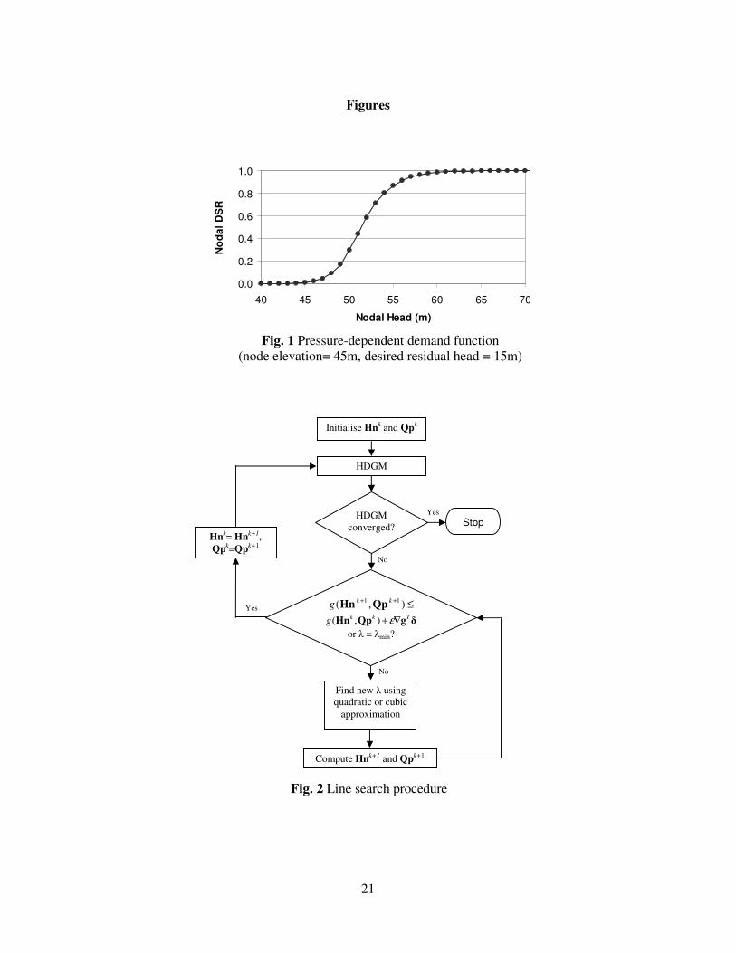
The basic form of the function is illustrated in Fig. 1 in which the demand satisfaction
ratio (DSR) is Qni(Hni)/Qnireq
. It is worth observing the smooth transition between
zero and partial nodal flow and between partial and full demand satisfaction. Further
details of this function can be found in Tanyimboh and Templeman (2010).
(Fig.1 here)
3 Pressure Dependent Demand Model
This section describes the extension of the Global Gradient Method (GGM) to include
demands that are pressure dependent. In the original GGM, the two conservation
equations, namely mass balance at nodes and energy conservation along hydraulic
links are solved simultaneously as
−
−
=
req
010
21
1211
Qn
HA
Hn
Qp
0A
AA
LL
M
LLL
M
(6a)
where A11 represents the diagonal matrix whose elements are the
jj
n
jj QpmQpQpK /))(( 2+ for pipes and j
n
jj QpQpKh /))/(( 0
2 ωω −− for pumps. Kj
and n are the resistance coefficient and flow exponent in the head loss formula
respectively. h0 is the shutoff head for the pump. m and ω are the minor loss and
pump curve coefficients respectively. Qpj is the flow rate in pipe j. The overall
incidence matrix relating the pipes to nodes with unknown and known heads is
represented by A12 and A10 respectively. Pipe flow leaving node is defined as -1, pipe
flow into node as +1 and 0 if pipe is not connected to node. A21 is the transpose of
A12. Qp denotes the column vector of unknown pipe flow rates. Hn and H0 are
6
column vectors for unknown and known nodal heads respectively. Qnreq
is the
column vector for required nodal supplies.
The continuity equation from Eq. 6a, i.e. 0=+ req
21 QnQpA shows that the sum of
flows flowing in and out of the demand node (i.e. A21Qp) is always equal to the
required nodal supply. In other words, the nodal demand is assumed to be fully
satisfied at all times. In pressure dependent analysis, the nodal outflow is pressure
dependent and will not be fully satisfied if the available pressure is insufficient.
Hence, the sum of pipe flows in and out of the demand node will not always be equal
to the required supply. To incorporate pressure dependent demand, Qnreq
is replaced
with Qn(Hn) where Qn(Hn) represents the pressure dependent nodal flow which is
estimated using the Tanyimboh and Templeman (2004) function herein. A diagonal
matrix A22 is introduced into Eq. 6a to form
−
=
0
HA
Hn
Qp
AA
AA 010
2221
1211
LL
M
LLL
M
(6b)
where the elements of the diagonal matrix A22 are Qn(Hn)/Hn.
Eq. 6b is then differentiated with respect to the pipe discharges and nodal heads to
give
=
dq
dE
dHn
dQp
DA
AD
2221
1211
LL
M
LLL
M
(7)
where the elements of diagonal matrix D11 can be written as j
n
jj QpmQpnK 21
+−
for
pipes and 12 )/( −n
jj QpKn ωω for pumps. D22 represents a diagonal matrix whose
elements are the derivatives of Qn(Hn) which is expressed as 2))exp(1()exp( −++⋅+⋅⋅ iiiiii
req
i HnHnQn βαβαβ . dQp and dHn represent the
corrective steps for Qp and Hn, respectively, in successive iterations and can be
defined as
kk QpQpdQp −= +1 (8)
kk HnHndHn −= +1 (9)
in which k represents the iteration number. The computational solution scheme for Eq.
6b is based on successive linearization using a first order Taylor series expansion
from which it can be shown that dE and dq represent the energy conservation and
mass balance equations respectively. Therefore, with reference to Eq. 6b,
0HAHnAQpAdE 101211 ++= (10)
7
HnAQpAdq 2221 += (11)
By substituting Eq. 10 and Eq. 11 into Eq. 7, the iterative procedure for solving Eq.
6b is obtained as follows.
FAHn 11 −+ =k (12)
01011211111212221 HADAQpADAHnDQn(HnQpAF 11) −− −−−+= kkkk (13)
22121121 DADAA −= −1 (14)
)( 111
010121111 HAHnAQpADQpQp ++−= +−+ kkkk (15)
Hence the algorithm first updates the nodal heads Hn by calculating Hnk+1
(Eqs. 12-
14) before updating the pipe flow rates Qp by calculating Qpk+1
(Eq. 15). Detailed
derivations of Eqs. 12-15 and further details regarding matrices A11, A12, A21 and A10
can be found in Rossman (2002) and Salgado et al. (1993).
4 Backtracking and Line Search Procedure
The integration of the HFR into the system of hydraulic equations is really a
complicated task. One major challenge encountered in doing so is the deterioration of
the GGM algorithm’s excellent convergence property. To include a HFR into the
mass balance equations would further increase the overall non-linearity of the system
of equations and render it more complex and difficult to solve. Directly applying the
corrective steps obtained from the iterative solution methods for non-linear systems of
equations would not be sufficient. For example, Newton’s method often fails to
converge if the starting point (i.e. the initial estimate) is not close to a solution. A
globally convergent strategy that yields a solution from almost any starting point is
essentially required.
Giustolisi et al. (2008a) adopted a heuristic approach in their pressure-driven network
simulation model whereby an over-relaxation parameter that adjusts the Newton step
consisting of both pipe-flow and nodal-head corrections is increased or decreased
depending on the errors in the mass and energy balance equations. In the Head-Driven
Simulation Model developed by Tabesh et al. (2002), convergence is ensured by using
a step length adjustment parameter. However, its value is obtained by means of trial
and error.
Tanyimboh and Templeman (2010) utilized the backtracking and line search routine
in their PDA program PRAAWDS to guide the Newton search in the right direction
and ensure global convergence for the system of non-linear equations. It determines
the appropriate Newton step size in a deterministic manner, ensuring both the energy
and mass conservation functions are sufficiently improved in successive iterations. No
trial runs or parameter calibrations were required. Experience with PRAAWDS has
shown that the backtracking and line search routine is efficient and reliable. For this
8
reason, EPANET-PDX has utilised this technique in enhancing its convergence
properties.
The backtracking and line search routine used herein has been adapted from Press et
al. (1992). The following section describes our implementation of the backtracking
and line search procedure in the integration of the Tanyimboh and Templeman (2004)
nodal head-flow function within the GGM. Equations 10 and 11 for conservation of
energy and conservation of mass, respectively, can be re-written as
0101211 HAHnAQpAHnQpdE ++=),( (16)
HnAQpAHnQpdq 2221 +=),( (17)
Together, Eq. 16 and Eq. 17 form a single system of simultaneous nonlinear equations
hereinafter referred to as G(Qp,Hn) the solution of which is required. Accordingly,
[ ]TdqdEG M≡ and, from Eq. 6b, it can be seen that G(Qp,Hn) = 0 at the solution.
The aim of the backtracking and line search procedure is to ensure that the function
GGHnQp Tg =),( decreases sufficiently in each iteration of the computational
solution algorithm so that, at the solution, g = 0.
In order to incorporate the backtracking and line search procedure the nodal heads Hn
are updated iteratively as
δHnHnHn ⋅+=+ λkk 1 (18)
where the scalar parameter λ is an over-relaxation coefficient that satisfies 10 ≤< λ
and k represents the iteration number. δHn is the full Newton step for the nodal heads Hn. Upon substituting the newly obtained nodal heads Hn
k+1 into Eq. 15, the
new pipe flows Qpk+1
are obtained.
To ensure that the function g, a scalar, has decreased sufficiently, a prescribed
minimum reduction in g is enforced to ensure that at least a fraction ε of the initial
rate of reduction in g in the Newton direction δ= T][ δHnδQpM is achieved. The initial
rate of reduction in g at the current iterate Tkk ][ HnQp M is TT ][ δHnδQpg M∇ in which
g∇ is the gradient of g. Therefore, the acceptance criterion for the next iterate Tkk ][ 11 ++ HnQp M is
TkkkkTTkkkkkk gg )]()[(]),([),(),( 1111 HnHnQpQpHnQpgHnQpHnQp −−∇+≤ ++++
Mε
(19)
where the scalar parameter ε satisfies 10 << ε ; we used ε =10-4
(Press et al. 1992).
In EPANET-PDX, to exploit the quadratic convergence of the GGM algorithm near
the solution, the full Newton step δ= T][ δHnδQpM , i.e. λ = 1 in Eq. 18, is always tried
first. However, if the full Newton step given by λ = 1 in Eq. 18 is unsatisfactory, i.e.
),( 11 ++ kkg HnQp does not meet the acceptance criterion in Eq. 19, that is to say
9
),(),( 11 ++− kkkk gg HnQpHnQp is not large enough and thus g has not decreased
sufficiently, backtracking along the Newton direction δ is carried out. The first
backward step or backtrack along the Newton direction δ is effected by modelling
)(),( 11 λgg kk ≡++ HnQp as a quadratic function of λ using the substitution 1+kHn =
δHnHn ⋅+ λk . The value of λ that minimizes the function g is then obtained which, therefore, yields Hn
k+1 and Qp
k+1. If more backtracking is necessary, then, for the
second and any subsequent backtracks, g(λ) is modelled as a cubic function of λ . The
backtracking procedure continues until either Eq. 19 is satisfied or λ reaches the
minimum set value minλ . We set a minimum value of 2.0min =λ to stop the algorithm
from taking steps that are too small as this would result in a large number of iterations
and consequently a longer computational time.
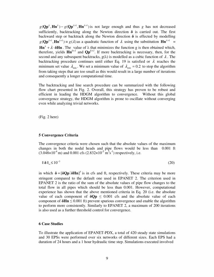
The backtracking and line search procedure can be summarized with the following
flow chart presented in Fig. 2. Overall, this strategy has proven to be robust and
efficient in leading the HDGM algorithm to convergence. Without this global
convergence strategy, the HDGM algorithm is prone to oscillate without converging
even while analyzing trivial networks.
(Fig. 2 here)
5 Convergence Criteria
The convergence criteria were chosen such that the absolute values of the maximum
changes in both the nodal heads and pipe flows would be less than 0.001 ft
(3.048×10⁻⁴
m) and 0.001 cfs (2.832×10⁻⁵
m3s
-1) respectively, i.e.
310|||| −
∞ ≤δ (20)
in which T][ δHnδQpδ M= is in cfs and ft, respectively. These criteria may be more
stringent compared to the default one used in EPANET 2. The criterion used in
EPANET 2 is the ratio of the sum of the absolute values of pipe flow changes to the
total flow in all pipes which should be less than 0.001. However, computational
experience has shown that the above mentioned criteria in Eq. 20 (i.e. the absolute
value of each component of δQp ≤ 0.001 cfs and the absolute value of each
component of δHn ≤ 0.001 ft) prevent spurious convergence and enable the algorithm
to perform more consistently. Similarly to EPANET 2, a maximum of 200 iterations
is also used as a further threshold control for convergence.
6 Case Studies
To illustrate the application of EPANET-PDX, a total of 420 steady state simulations
and 30 EPSs were performed over six networks of different sizes. Each EPS had a
duration of 24 hours and a 1 hour hydraulic time step. Simulations executed involved
10
1) Varying the source heads thus subjecting the networks to the entire range of
DSRs; and
2) Randomly closing pipes to create stress within the networks.
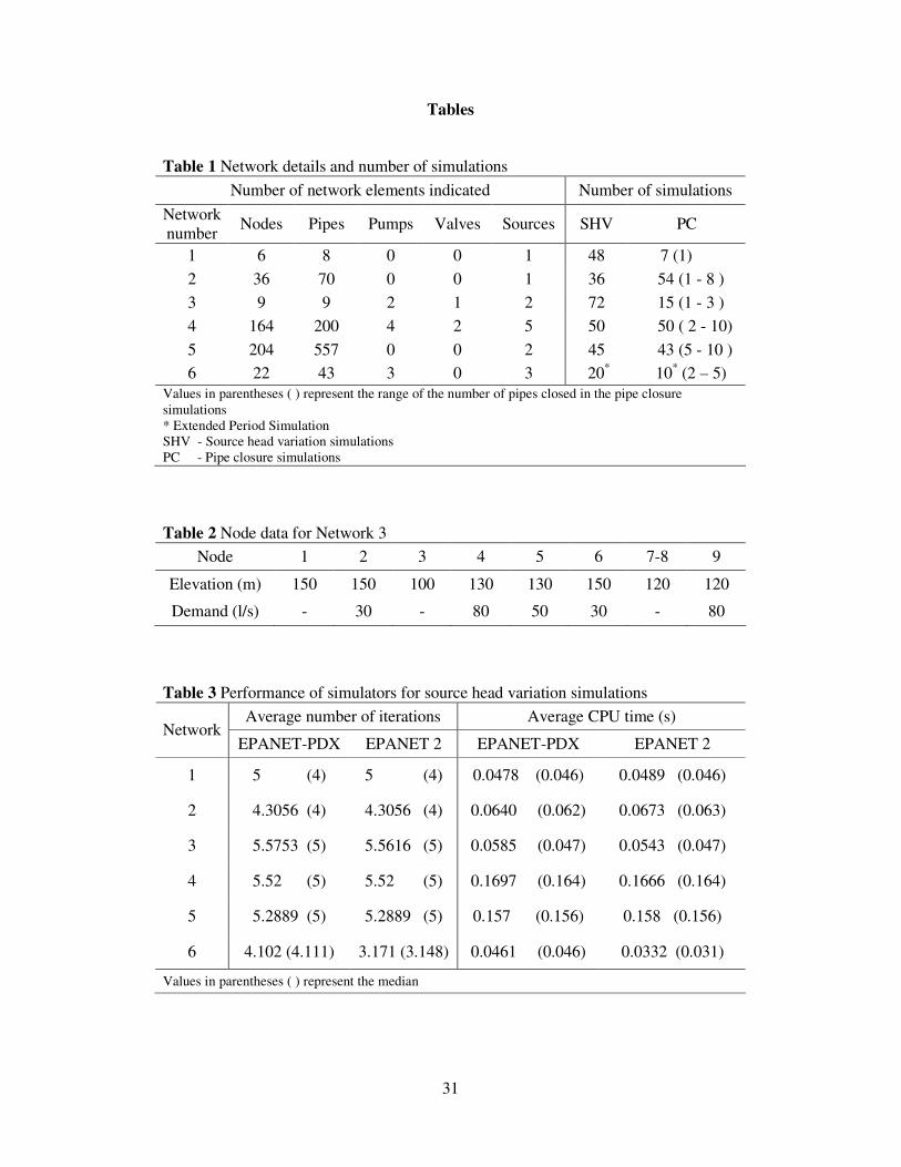
Table 1 shows the characteristics of the networks along with the numbers and types of
simulation carried out. Under the pipe closure (PC) simulation column in Table 1,
values in parentheses represent the number of pipes closed. For example, the number
of pipes closed for network 2 ranged from 1 pipe to 8 pipes. Also, EPANET 2 was run
concurrently for each simulation to serve as comparison for both PDA and DDA.
Thus overall, 840 steady state and 60 EPS simulations were involved in this
assessment. Additional EPANET 2 simulations were carried out to verify the accuracy
of the PDA results as detailed later in the “results verification” in Section 8.
(Table 1 here)
Overall, the performances of EPANET-PDX and EPANET 2 were very similar as
shown herein. Consequently, not all aspects of results will be presented for every
network. However, detailed results of the simulators’ performance on the whole in
terms of robustness, average CPU time and number of iterations are presented and
discussed at the end of the paper.
It is essential to clarify two key terms which will be extensively used in the following
section of the paper. The term demand satisfaction ratio (DSR) represents the ratio of
the available nodal flow to the nodal demand and takes values between 0 and 1. A
network DSR value of 0.5 means only 50% of the total network demand is satisfied. It
is also worth mentioning that DSRs for nodes and networks are only presented for
EPANET-PDX and not EPANET 2. The reason is EPANET 2 is a DDA based
hydraulic simulator and hence the nodal demands are implicitly assumed to be
satisfied in full regardless of whether the pressure is sufficient or not. The second
term, nodal residual pressure head refers to the pressure head of the node excluding
the elevation.
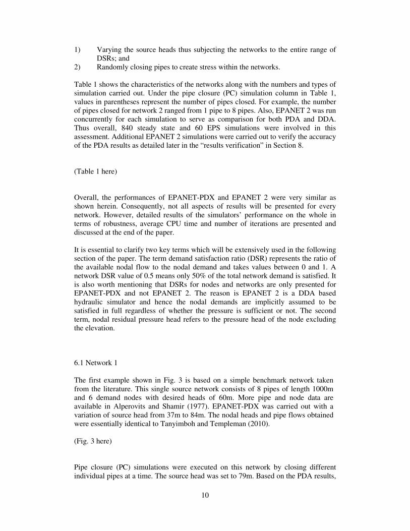
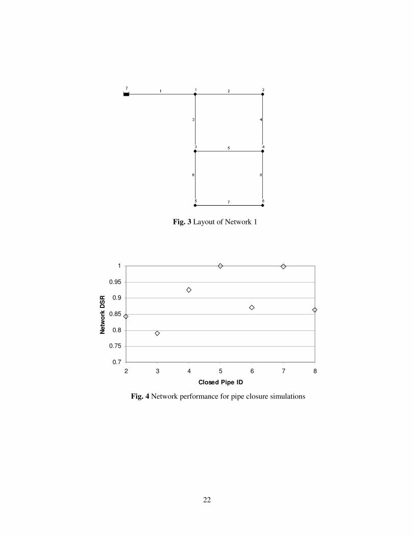
6.1 Network 1
The first example shown in Fig. 3 is based on a simple benchmark network taken
from the literature. This single source network consists of 8 pipes of length 1000m
and 6 demand nodes with desired heads of 60m. More pipe and node data are
available in Alperovits and Shamir (1977). EPANET-PDX was carried out with a
variation of source head from 37m to 84m. The nodal heads and pipe flows obtained
were essentially identical to Tanyimboh and Templeman (2010).
(Fig. 3 here)
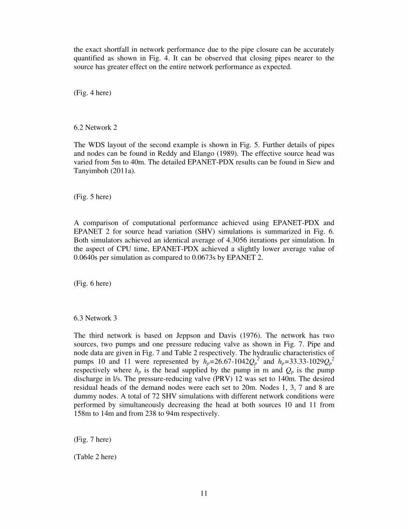
Pipe closure (PC) simulations were executed on this network by closing different
individual pipes at a time. The source head was set to 79m. Based on the PDA results,
11
the exact shortfall in network performance due to the pipe closure can be accurately
quantified as shown in Fig. 4. It can be observed that closing pipes nearer to the
source has greater effect on the entire network performance as expected.
(Fig. 4 here)
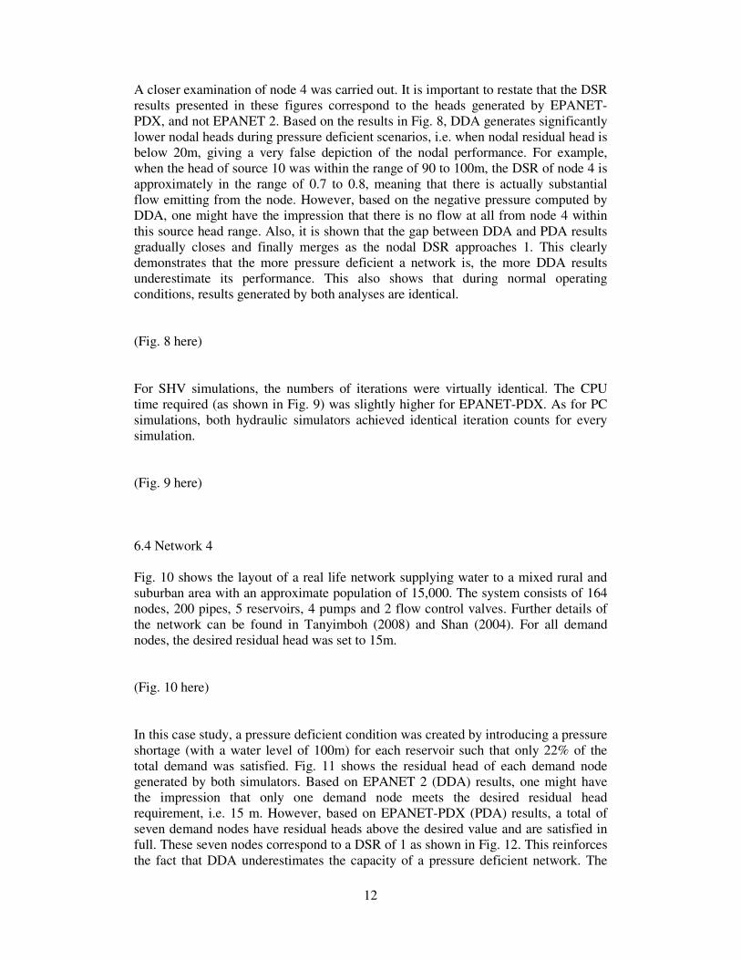
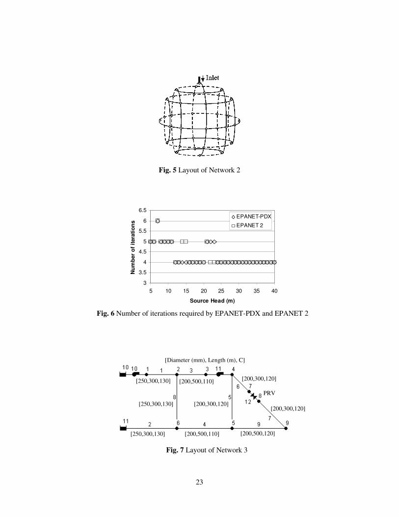
6.2 Network 2
The WDS layout of the second example is shown in Fig. 5. Further details of pipes
and nodes can be found in Reddy and Elango (1989). The effective source head was
varied from 5m to 40m. The detailed EPANET-PDX results can be found in Siew and
Tanyimboh (2011a).
(Fig. 5 here)
A comparison of computational performance achieved using EPANET-PDX and
EPANET 2 for source head variation (SHV) simulations is summarized in Fig. 6.
Both simulators achieved an identical average of 4.3056 iterations per simulation. In
the aspect of CPU time, EPANET-PDX achieved a slightly lower average value of
0.0640s per simulation as compared to 0.0673s by EPANET 2.
(Fig. 6 here)
6.3 Network 3
The third network is based on Jeppson and Davis (1976). The network has two
sources, two pumps and one pressure reducing valve as shown in Fig. 7. Pipe and
node data are given in Fig. 7 and Table 2 respectively. The hydraulic characteristics of
pumps 10 and 11 were represented by hp=26.67-1042Qp2 and hp=33.33-1029Qp
2
respectively where hp is the head supplied by the pump in m and Qp is the pump
discharge in l/s. The pressure-reducing valve (PRV) 12 was set to 140m. The desired
residual heads of the demand nodes were each set to 20m. Nodes 1, 3, 7 and 8 are
dummy nodes. A total of 72 SHV simulations with different network conditions were
performed by simultaneously decreasing the head at both sources 10 and 11 from
158m to 14m and from 238 to 94m respectively.
(Fig. 7 here)
(Table 2 here)
12
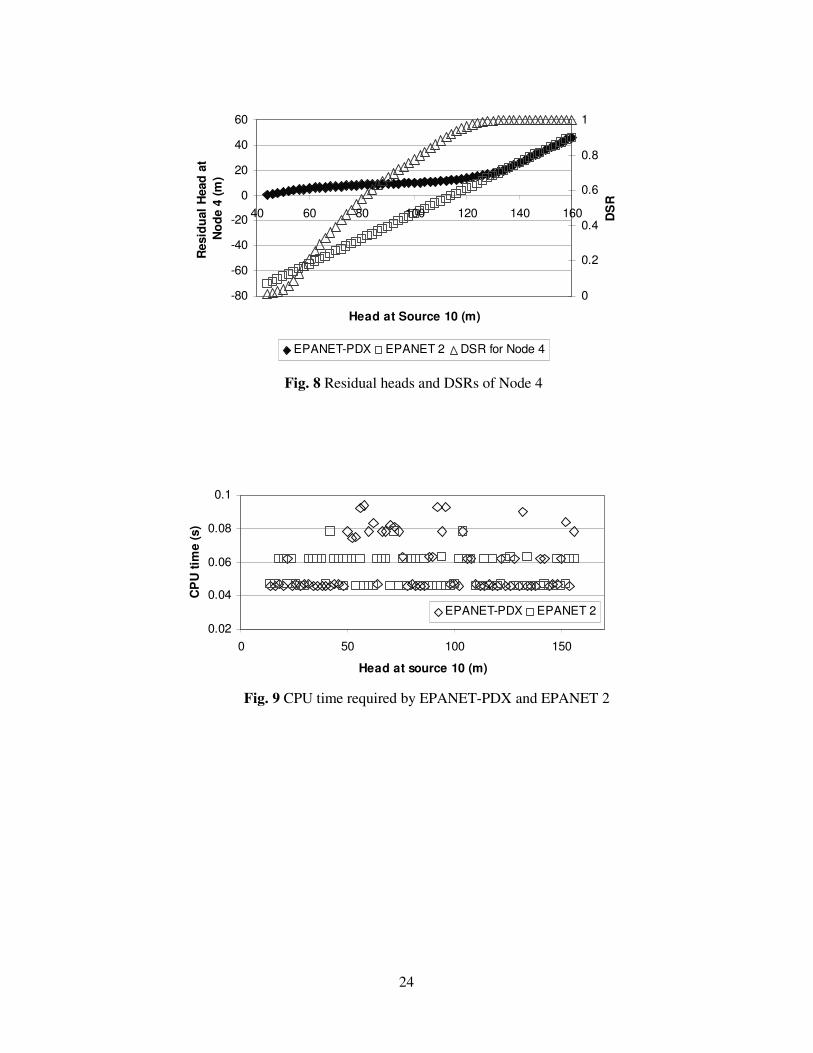
A closer examination of node 4 was carried out. It is important to restate that the DSR
results presented in these figures correspond to the heads generated by EPANET-
PDX, and not EPANET 2. Based on the results in Fig. 8, DDA generates significantly
lower nodal heads during pressure deficient scenarios, i.e. when nodal residual head is
below 20m, giving a very false depiction of the nodal performance. For example,
when the head of source 10 was within the range of 90 to 100m, the DSR of node 4 is
approximately in the range of 0.7 to 0.8, meaning that there is actually substantial
flow emitting from the node. However, based on the negative pressure computed by
DDA, one might have the impression that there is no flow at all from node 4 within
this source head range. Also, it is shown that the gap between DDA and PDA results
gradually closes and finally merges as the nodal DSR approaches 1. This clearly
demonstrates that the more pressure deficient a network is, the more DDA results
underestimate its performance. This also shows that during normal operating
conditions, results generated by both analyses are identical.
(Fig. 8 here)
For SHV simulations, the numbers of iterations were virtually identical. The CPU
time required (as shown in Fig. 9) was slightly higher for EPANET-PDX. As for PC
simulations, both hydraulic simulators achieved identical iteration counts for every
simulation.
(Fig. 9 here)
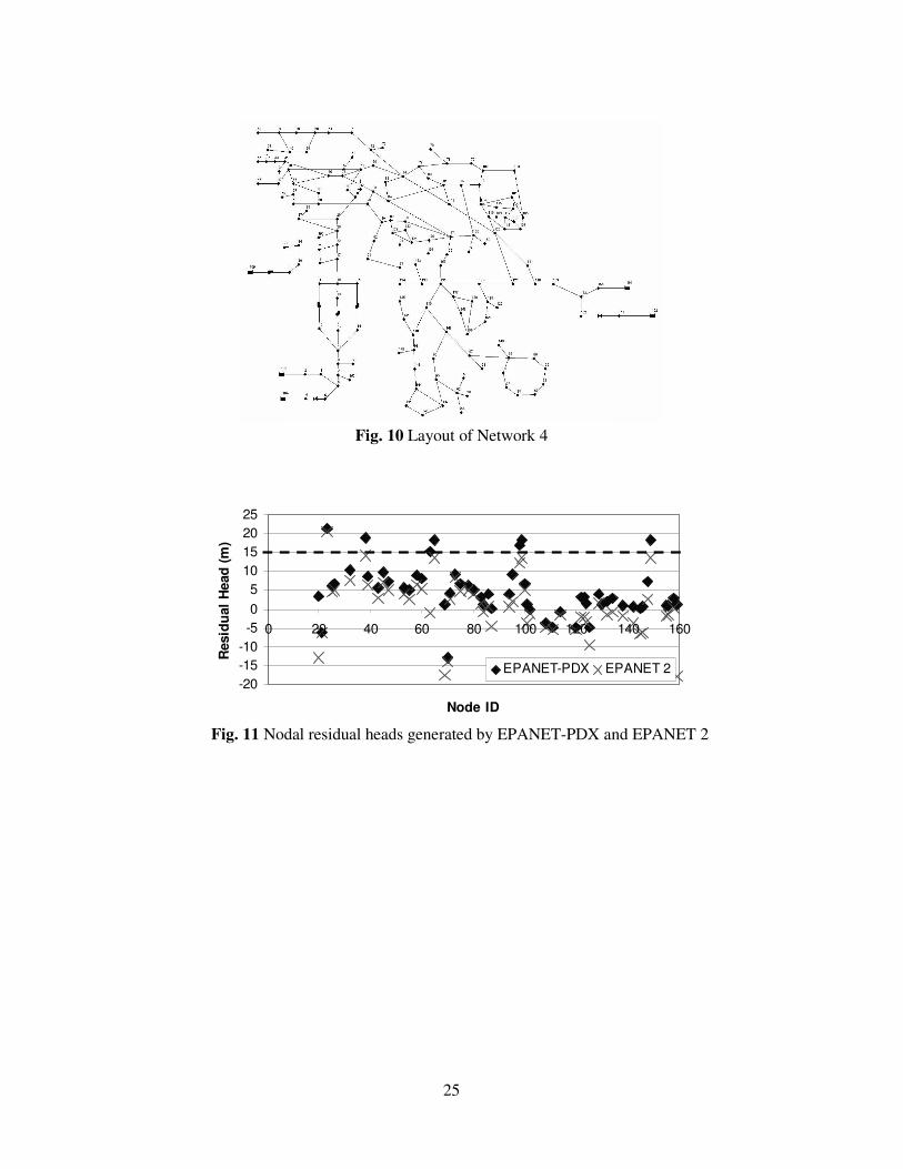
6.4 Network 4
Fig. 10 shows the layout of a real life network supplying water to a mixed rural and
suburban area with an approximate population of 15,000. The system consists of 164
nodes, 200 pipes, 5 reservoirs, 4 pumps and 2 flow control valves. Further details of
the network can be found in Tanyimboh (2008) and Shan (2004). For all demand
nodes, the desired residual head was set to 15m.
(Fig. 10 here)
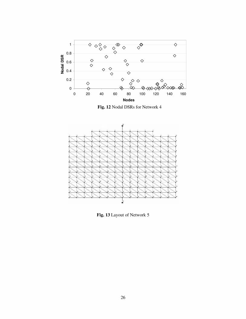
In this case study, a pressure deficient condition was created by introducing a pressure
shortage (with a water level of 100m) for each reservoir such that only 22% of the
total demand was satisfied. Fig. 11 shows the residual head of each demand node
generated by both simulators. Based on EPANET 2 (DDA) results, one might have
the impression that only one demand node meets the desired residual head
requirement, i.e. 15 m. However, based on EPANET-PDX (PDA) results, a total of
seven demand nodes have residual heads above the desired value and are satisfied in
full. These seven nodes correspond to a DSR of 1 as shown in Fig. 12. This reinforces
the fact that DDA underestimates the capacity of a pressure deficient network. The
13
performance of each demand node can be accurately assessed based on the nodal
demand satisfaction ratio (DSR) shown in Fig. 12. It is worth mentioning that nodes 1
to 19 have no demand and thus are not shown in both Fig. 11 and Fig. 12.
(Fig. 11 here)
(Fig. 12 here)
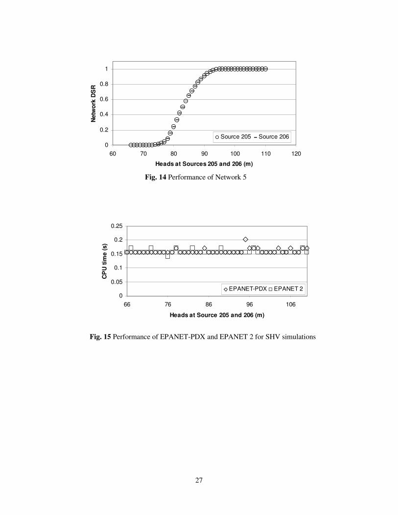
6.5 Network 5
The fifth example (Fig. 13) is a generic network (Shan, 2004) which consists of 204
nodes, 557 pipes and 2 reservoirs. All nodal elevations, required heads and demands
were 75m, 90m and 10 l/s respectively. All pipe lengths, diameters and Hazen-
Williams roughness coefficients were 100m, 0.45m and 130 respectively. A total of
45 PDA simulations were executed with heads at both reservoirs 205 and 206 varying
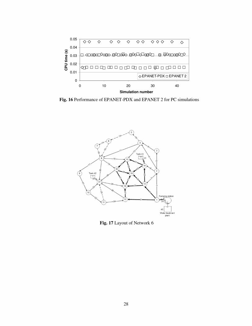
uniformly from 66m to 110m. The network performance is summarised in Fig. 14.
The performance of EPANET-PDX remains on a par with EPANET 2 even for large
networks as shown in Fig. 15 and Fig. 16.
(Fig. 13 here)
(Fig. 14 here)
(Fig. 15 here)
(Fig. 16 here)
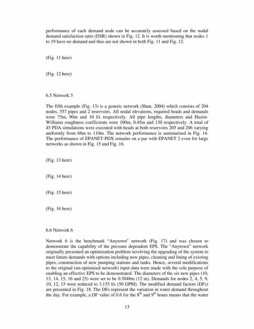
6.6 Network 6
Network 6 is the benchmark “Anytown" network (Fig. 17) and was chosen to
demonstrate the capability of the pressure dependent EPS. The “Anytown” network
originally presented an optimization problem involving the upgrading of the system to
meet future demands with options including new pipes, cleaning and lining of existing
pipes, construction of new pumping stations and tanks. Hence, several modifications
to the original (un-optimized network) input data were made with the sole purpose of
enabling an effective EPS to be demonstrated. The diameters of the six new pipes (10,
13, 14, 15, 16 and 25) were set to be 0.3048m (12 in). Demands for nodes 2, 4, 5, 9,
10, 12, 15 were reduced to 3.155 l/s (50 GPM). The modified demand factors (DFs)
are presented in Fig. 18. The DFs represent the variation in water demand throughout
the day. For example, a DF value of 0.6 for the 8th
and 9th
hours means that the water
14
consumption during both these hours is 0.6 times the average water use. The rest of
the network data remain the same as used in Walski et al. (1987).
(Fig. 17 here)
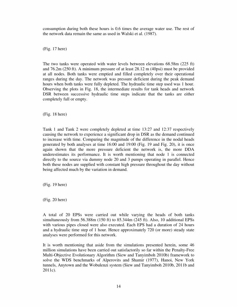
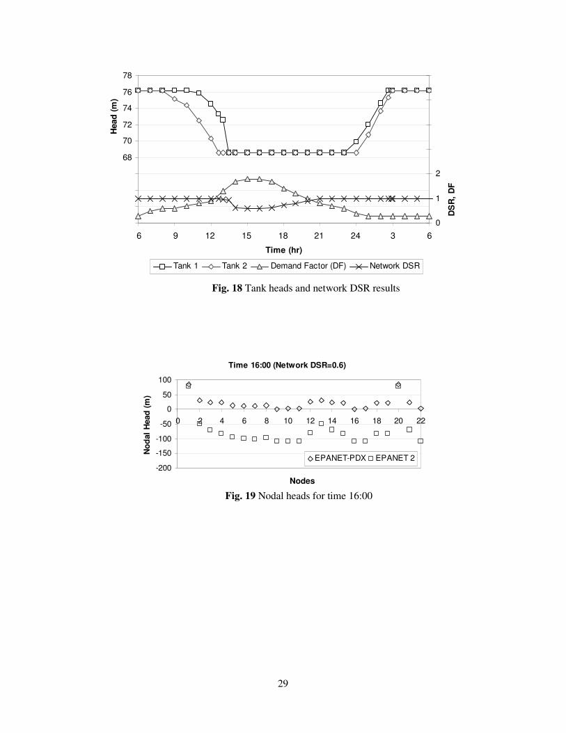
The two tanks were operated with water levels between elevations 68.58m (225 ft)
and 76.2m (250 ft). A minimum pressure of at least 28.12 m (40psi) must be provided
at all nodes. Both tanks were emptied and filled completely over their operational
ranges during the day. The network was pressure deficient during the peak demand
hours when both tanks were fully depleted. The hydraulic time step used was 1 hour.
Observing the plots in Fig. 18, the intermediate results for tank heads and network
DSR between successive hydraulic time steps indicate that the tanks are either
completely full or empty.
(Fig. 18 here)
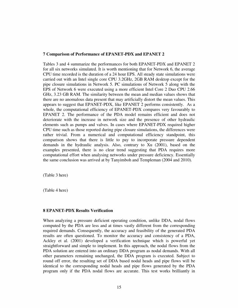
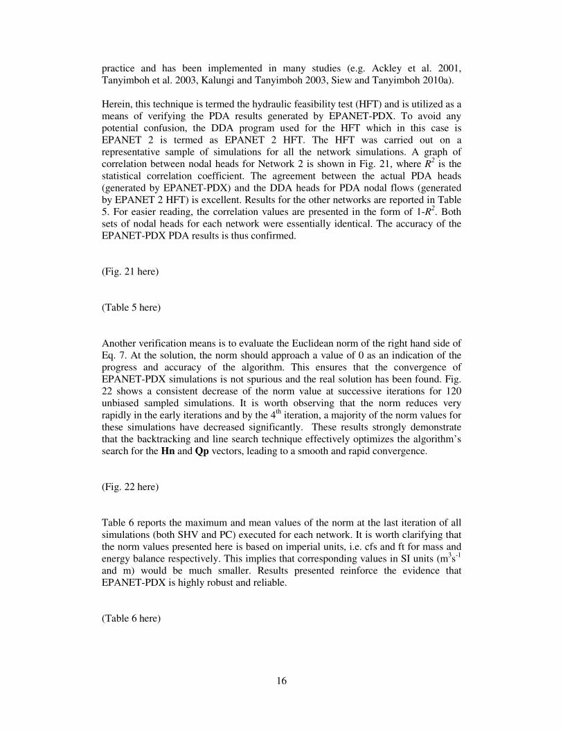
Tank 1 and Tank 2 were completely depleted at time 13:27 and 12:37 respectively
causing the network to experience a significant drop in DSR as the demand continued
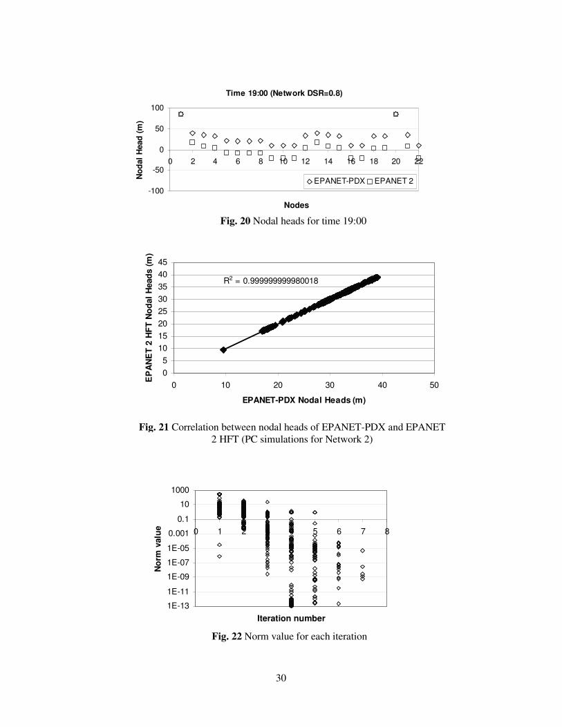
to increase with time. Comparing the magnitude of the difference in the nodal heads
generated by both analyses at time 16:00 and 19:00 (Fig. 19 and Fig. 20), it is once
again shown that the more pressure deficient the network is, the more DDA
underestimates its performance. It is worth mentioning that node 1 is connected
directly to the source via dummy node 20 and 3 pumps operating in parallel. Hence
both these nodes are supplied with constant high pressure throughout the day without
being affected much by the variation in demand.
(Fig. 19 here)
(Fig. 20 here)
A total of 20 EPSs were carried out while varying the heads of both tanks
simultaneously from 56.388m (150 ft) to 85.344m (245 ft). Also, 10 additional EPSs
with various pipes closed were also executed. Each EPS had a duration of 24 hours
and a hydraulic time step of 1 hour. Hence approximately 720 (or more) steady state
analyses were performed for this network.
It is worth mentioning that aside from the simulations presented herein, some 46
million simulations have been carried out satisfactorily so far within the Penalty-Free
Multi-Objective Evolutionary Algorithm (Siew and Tanyimboh 2010b) framework to
solve the WDS benchmarks of Alperovits and Shamir (1977), Hanoi, New York
tunnels, Anytown and the Wobulenzi system (Siew and Tanyimboh 2010b, 2011b and
2011c).
15
7 Comparison of Performance of EPANET-PDX and EPANET 2
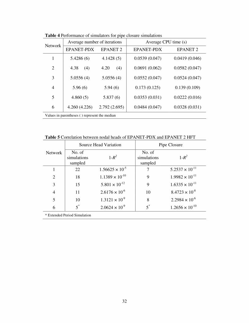
Tables 3 and 4 summarize the performances for both EPANET-PDX and EPANET 2
for all six networks simulated. It is worth mentioning that for Network 6, the average
CPU time recorded is the duration of a 24 hour EPS. All steady state simulations were
carried out with an Intel single core CPU 3.2GHz, 2GB RAM desktop except for the
pipe closure simulations in Network 5. PC simulations of Network 5 along with the
EPS of Network 6 were executed using a more efficient Intel Core 2 Duo CPU 2.66
GHz, 3.23 GB RAM. The similarity between the mean and median values shows that
there are no anomalous data present that may artificially distort the mean values. This
appears to suggest that EPANET-PDX, like EPANET 2 performs consistently. As a
whole, the computational efficiency of EPANET-PDX compares very favourably to
EPANET 2. The performance of the PDA model remains efficient and does not
deteriorate with the increase in network size and the presence of other hydraulic
elements such as pumps and valves. In cases where EPANET-PDX required higher
CPU time such as those reported during pipe closure simulations, the differences were
rather trivial. From a numerical and computational efficiency standpoint, this
comparison shows that there is little to pay to incorporate pressure dependent
demands in the hydraulic analysis. Also, contrary to Xu (2001), based on the
examples presented, there is no clear trend suggesting that PDA requires more
computational effort when analysing networks under pressure deficiency. Essentially
the same conclusion was arrived at by Tanyimboh and Templeman (2004 and 2010).
(Table 3 here)
(Table 4 here)
8 EPANET-PDX Results Verification
When analyzing a pressure deficient operating condition, unlike DDA, nodal flows
computed by the PDA are less and at times vastly different from the corresponding
required demands. Consequently, the accuracy and feasibility of the generated PDA
results are often questioned. To monitor the accuracy and consistency of a PDA,
Ackley et al. (2001) developed a verification technique which is powerful yet
straightforward and simple to implement. In this approach, the nodal flows from the
PDA solution are entered into an ordinary DDA program as nodal demands. With all
other parameters remaining unchanged, the DDA program is executed. Subject to
round off error, the resulting set of DDA based nodal heads and pipe flows will be
identical to the corresponding nodal heads and pipe flows generated by the PDA
program only if the PDA nodal flows are accurate. This test works brilliantly in
16
practice and has been implemented in many studies (e.g. Ackley et al. 2001,
Tanyimboh et al. 2003, Kalungi and Tanyimboh 2003, Siew and Tanyimboh 2010a).
Herein, this technique is termed the hydraulic feasibility test (HFT) and is utilized as a
means of verifying the PDA results generated by EPANET-PDX. To avoid any
potential confusion, the DDA program used for the HFT which in this case is
EPANET 2 is termed as EPANET 2 HFT. The HFT was carried out on a
representative sample of simulations for all the network simulations. A graph of
correlation between nodal heads for Network 2 is shown in Fig. 21, where R2 is the
statistical correlation coefficient. The agreement between the actual PDA heads
(generated by EPANET-PDX) and the DDA heads for PDA nodal flows (generated
by EPANET 2 HFT) is excellent. Results for the other networks are reported in Table
5. For easier reading, the correlation values are presented in the form of 1-R2. Both
sets of nodal heads for each network were essentially identical. The accuracy of the
EPANET-PDX PDA results is thus confirmed.
(Fig. 21 here)
(Table 5 here)
Another verification means is to evaluate the Euclidean norm of the right hand side of
Eq. 7. At the solution, the norm should approach a value of 0 as an indication of the
progress and accuracy of the algorithm. This ensures that the convergence of
EPANET-PDX simulations is not spurious and the real solution has been found. Fig.
22 shows a consistent decrease of the norm value at successive iterations for 120
unbiased sampled simulations. It is worth observing that the norm reduces very
rapidly in the early iterations and by the 4th
iteration, a majority of the norm values for
these simulations have decreased significantly. These results strongly demonstrate
that the backtracking and line search technique effectively optimizes the algorithm’s
search for the Hn and Qp vectors, leading to a smooth and rapid convergence.
(Fig. 22 here)
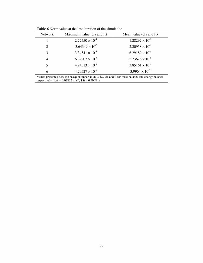
Table 6 reports the maximum and mean values of the norm at the last iteration of all
simulations (both SHV and PC) executed for each network. It is worth clarifying that
the norm values presented here is based on imperial units, i.e. cfs and ft for mass and
energy balance respectively. This implies that corresponding values in SI units (m3s
-1
and m) would be much smaller. Results presented reinforce the evidence that
EPANET-PDX is highly robust and reliable.
(Table 6 here)
17
9 Conclusions
A comprehensive study on PDA and DDA involving a total of 1385 steady state
simulations and 70 24-hour EPSs has been carried out. Results presented herein
demonstrate that EPANET-PDX is robust, efficient and accurate in analyzing both
normal and pressure deficient conditions. In terms of computational efficiency, the
performance of EPANET-PDX compares very favourably to EPANET 2. With this
said, one should bear in mind that EPANET 2 results are inaccurate, misleading or
infeasible while analysing pressure deficient networks as demonstrated clearly in the
paper. This new EPANET-PDX model provides a fully equipped pressure dependent
extended period simulation and is capable of simulating real world networks with
tanks, pumps and valves. Evidence of its robustness includes the ability to produce
realistic, hydraulically consistent results for the entire range of network demand
satisfaction from zero to 100% without any convergence complications. Indeed in all
of the cases attempted so far, there is no instance where the program failed to
converge.
The accuracy of the generated PDA results has been validated and verified using the
hydraulic feasibility test and evaluation of the energy and mass balance errors at the
solution. Results presented demonstrate the drawbacks of DDA which include the
exaggeration of pressure shortage and the inability to quantify the deficiency of the
network performance. From a computational standpoint, the backtracking and line
search procedure has proven to be effective in providing robustness and very efficient
convergence of the hydraulic simulation model. The development of EPANET-PDX
has enabled PDA to be used successfully in WDS optimization and the initial results
can be found in Siew and Tanyimboh (2010b).
Given the excellent computational properties of EPANET 2, the results herein
demonstrate that the performance of EPANET-PDX is essentially on a par with the
conventional demand driven approach. Some issues not addressed in this paper
include other pressure-dependent nodal flow functions (i.e. HFRs) and integrated
pressure-dependent water quality modelling. Also, a comparison between EPANET-
PDX and other PDA approaches such as Ackley et al. (2001), Giustolisi et al.
(2008a,b) and OOTEN (a public-domain object-oriented toolkit for EPANET) is not
included. More work on these and other aspects is indicated.
Acknowledgements
This research was funded in part by the UK Engineering and Physical Sciences
Research Council under Grant Number EP/G055564/1. The authors are grateful to the
British Government (Overseas Research Students Award Scheme) and the University
of Strathclyde for funding for the first author’s PhD programme.
18
References
Ackley JRL, Tanyimboh TT, Tahar B, Templeman AB (2001) Head-driven analysis
of water distribution systems. Water Software Systems: Theory and Applications,
Vol. 1, Ulanicki, B., Coulbeck, B. and Rance, J. (eds.), Research Studies Press
Ltd, England, ISBN 0863802745, Chapter 3:183-192
Alperovits E, Shamir U (1977) Design of optimal water distribution systems. Water
Resources Research 13(6):885-900
Ang WH, Jowitt PW (2006) Solution for water distribution systems under pressure-
deficient conditions. Journal of Water Resources Planning and Management,
ASCE 132(3):175-182
Bhave PR, (1991) Analysis of Flow in Water Distribution Networks. Lancaster, PA:
Technomic Publishing
Cisty M (2010) Hybrid genetic algorithm and linear programming method for least-
cost design of water distribution systems. Water Resources Management, 24(1):
1–24
Christodoulou SE (2010) Water network assessment and reliability analysis by use
of survival analysis. Water Resources Management, 25(4): 1229–1238
Cullinane MJ, Lansey KE, Mays LW (1992) Optimisation-availability-based design
of water distribution networks. Journal of Hydraulics Engineering 118(3):420-441
Fujiwara O, Ganesharajah T (1993) Reliability assessment of water supply systems
with storage and distribution networks. Water Resource Research 29(8):2917-
2924.
Germanopoulos G (1985) A technical note on the inclusion of pressure dependent
demand and leakage terms in water supply network models. Civil Engineering
Systems 2:171-179
Giustolisi O, Kapelan Z, Savic DA (2008a) Extended period simulation analysis
considering valve shutdowns. Journal of Water Resource Planning and
Management 134(6):527-537
Giustolisi O, Savic DA, Kapelan Z (2008b) Pressure-driven demand and leakage
simulation for water distribution networks. Journal of Hydraulic Engineering
134(5):626-635
Gupta R, Bhave PR (1996) Comparison of methods for predicting deficient network
performance. Journal of Water Resource Planning and Management 122(3):214-
217
Haghighi A, Samani HMV, Samani ZMV (2011) GA-ILP method for optimization of
water distribution networks. Water Resources Management 25(7): 1791–1808
Jeppson RW, Davis A (1976) Pressure reducing valves in pipe network analyses.
Journal of Hydraulics Division 102(HY7):987-1001
Kalungi P, Tanyimboh TT (2003) Redundancy model for water distribution systems.
Reliability Engineering and System Safety 82(3):275-286
Martínez-Rodríguez JB, Montalvo I, Izquierdo J, Pérez-García R (2011) Reliability
and Tolerance Comparison in Water Supply Networks. Water Resources
Management, 25(5):1437–1448
Liberatore S, Sechi GM (2009) Location and calibration of valves in water
distribution networks using a scatter-search meta-heuristic approach. Water
Resources Management, 23: 1479–1495
OFWAT (2004) Levels of Service for the Water Industry in England and Wales.
2002-2003 Report. Ofwat Centre, 7 Hill Street, Birmingham B5 4UA, UK
19
Park S, Choi CL, Kim JH, Bae CH (2010) Evaluating the economic residual life of
water pipes using the proportional hazards model. Water Resources Management,
24(12): 3195–3217
Press WH, Teukolsky SA, Vetterling WT, Flannery BP (1992) Numerical Recipes in
FORTRAN: The Art of Scientific Computing. Cambridge University Press, New
York, USA
Reddy LS, Elango K (1989) Analysis of water distribution networks with head
dependent outlets. Civil Engineering Systems 6(3):102-110
Rossman LA (2002) EPANET 2 User’s Manual, Water Supply and Water Resources
Division, National Risk Management Research Laboratory, Cincinnati, OH45268
Rossman LA (2007) Discussion of ‘Solution for water distribution systems under
pressure-deficient conditions’. Journal of Water Resources Planning and
Management 133(6):566-567
Salgado R, Rojo J, Zepeda S (1993) Extended gradient method for fully non-linear
head and flow analysis in pipe networks. Integrated Computer Applications in
Water Supply-- Methods and Procedures for Systems Simulation and Control, 1,
pp. 49-60
Shan N (2004) Head dependent modelling of water distribution network. MSc
Dissertation, University of Liverpool, UK
Siew C, Tanyimboh TT (2010a) Pressure-dependent EPANET extension: pressure-
dependent demands. Proceedings of the 12th
Annual Water Distribution Systems
Analysis Conference, WDSA 2010, September 12-15, Tucson, Arizona
Siew C, Tanyimboh TT (2010b) Penalty-Free Multi-Objective Evolutionary
Optimization of Water Distribution Systems. Proceedings of the 12th
Annual
Water Distribution Systems Analysis Conference, WDSA 2010, September 12-15,
Tucson, Arizona
Siew C, Tanyimboh TT (2011a) The computational efficiency of EPANET-PDX.
Proceedings of the 13th
Annual Water Distribution Systems Analysis Conference,
WDSA 2011, May 22-26, Palm Springs, California
Siew C, Tanyimboh TT (2011b) Design of the “Anytown” network using the penalty-
free multi-objective evolutionary optimization approach. Proceedings of the 13th
Annual Water Distribution Systems Analysis Conference, WDSA 2011, May 22-
26, Palm Springs, California
Siew C, Tanyimboh TT (2011c) Penalty-free evolutionary algorithm optimization for
the long term rehabilitation and upgrading of water distribution systems.
Proceedings of the 13th
Annual Water Distribution Systems Analysis Conference,
WDSA 2011, May 22-26, Palm Springs, California
Tabesh M, Tanyimboh TT, Burrows R (2002) Head driven simulation of water supply
networks. Int. J. Eng., Transactions A: Basics 15(1):11–22
Tabesh M, Yekta A, Burrows R (2009) An integrated model to evaluate losses in
water distribution systems. Water Resources Management, 23(3):477–492
Tanyimboh TT (2008) Robust algorithm for head-dependent analysis of water
distribution systems. Proceedings of the 10th
Annual Water Distribution Systems
Analysis Conference, Van Zyl, J.E., Ilemobade, A.A. and Jacobs, H.E. (eds.),
August 17-20, Kruger National Park, South Africa
Tanyimboh TT, Tahar B, Templeman AB (2003) Pressure-driven modelling of water
distribution systems. Water Science and Technology-Water Supply, 3(1-2):255-
262
Tanyimboh TT, Templeman AB (2004) A new nodal outflow function for water
distribution networks. Proceedings of the 4th
International Conf. on Eng.

20
Computational Technology, Topping, B.H.V. and Mota Soares, C.A. (eds.), Civil-
Comp Press, Stirling, UK, ISBN 0-948749-98-9, Paper 64, pp. 12, CD-ROM
Tanyimboh TT, Templeman AB (2010) Seamless pressure-deficient water
distribution system model. J. Water Management, ICE, 163(8):389-396
Todini E, Pilati S (1988) A gradient algorithm for the analysis of pipe networks.
Computer Applications in Water Supply, Volume 1, Coulbeck, B., and Orr, C-H
(eds.), Research Studies Press, England
Udo A, Ozawa T (2001) Steady-state flow analysis of pipe networks considering
reduction of flow in the case of low water pressures. Water Software Systems:
Theory and Applications (Ulanicki B, Coulbeck B and Rance J (eds.)). Research
Studies Press, Taunton, UK, Vol. 1, pp. 73-182
Wagner JM, Shamir U, Marks DH (1988) Water distribution reliability: simulation
methods. Journal of Water Resources Planning and Management, 114(3):276-294
Walski TM, Brill ED, Gessler J, Goulter IC, Jeppson RM, Lansey K, Lee HL,
Liebman JC, Mays L, Morgan DR, Ormsbee L (1987) Battle of the network
models: epilogue. Journal of Water Resource Planning and Management,
113(2):191-203
Wu YW, Wang RH, Walski TM, Yang SY, Bowdler D, Baggett CC (2009) Extended
global-gradient algorithm for pressure-dependent water distribution analysis.
Journal of Water Resource Planning and Management, 135(1):13-22
Xu C (2001) Re: modelling demands. www.bossintl.com/forums/showthr.../thread
id/5176.htm, June 2001, accessed 2002 by Tanyimboh and Templeman (2004)
21
Figures
0.0
0.2
0.4
0.6
0.8
1.0
40 45 50 55 60 65 70
Nodal Head (m)
No
da
l D
SR
Fig. 1 Pressure-dependent demand function (node elevation= 45m, desired residual head = 15m)
Initialise Hnk and Qpk
Compute Hnk+1 and Qpk+1
Stop
Hnk= Hnk+1,
Qpk=Qpk+1
Yes
Yes
No
No
≤++ ),( 11 kkg QpHn
δgQpHnTkk
g ∇+ ε),(
or λ = λmin?
Find new λ using
quadratic or cubic
approximation
HDGM
Fig. 2 Line search procedure
HDGM
converged?
22
Fig. 3 Layout of Network 1
0.7
0.75
0.8
0.85
0.9
0.95
1
2 3 4 5 6 7 8
Closed Pipe ID
Netw
ork
DS
R
Fig. 4 Network performance for pipe closure simulations
23
Fig. 5 Layout of Network 2
3
3.5
4
4.5
5
5.5
6
6.5
5 10 15 20 25 30 35 40
Source Head (m)
Nu
mb
er
of
itera
tio
ns
EPANET-PDX
EPANET 2
Fig. 6 Number of iterations required by EPANET-PDX and EPANET 2
Fig. 7 Layout of Network 3
[250,300,130] [200,500,110]
[200,300,120]
[200,300,120]
[200,500,120] [200,500,110] [250,300,130]
[200,300,120] [250,300,130]
[Diameter (mm), Length (m), C]
PRV
24
Fig. 8 Residual heads and DSRs of Node 4
-80
-60
-40
-20
0
20
40
60
40 60 80 100 120 140 160
Head at Source 10 (m)
Resid
ual
Head
at
No
de 4
(m
)
0
0.2
0.4
0.6
0.8
1
DS
R
EPANET-PDX EPANET 2 DSR for Node 4
0.02
0.04
0.06
0.08
0.1
0 50 100 150
Head at source 10 (m)
CP
U t
ime (
s)
EPANET-PDX EPANET 2
Fig. 9 CPU time required by EPANET-PDX and EPANET 2
25
Fig. 10 Layout of Network 4
-20
-15
-10
-5
0
5
10
15
20
25
0 20 40 60 80 100 120 140 160
Node ID
Resid
ual
Head
(m
)
EPANET-PDX EPANET 2
Fig. 11 Nodal residual heads generated by EPANET-PDX and EPANET 2
26
0
0.2
0.4
0.6
0.8
1
0 20 40 60 80 100 120 140 160
Node
No
dal
DS
R
Nodes
Fig. 12 Nodal DSRs for Network 4
Fig. 13 Layout of Network 5
27
0
0.05
0.1
0.15
0.2
0.25
66 76 86 96 106
Heads at Source 205 and 206 (m)
CP
U t
ime (
s)
EPANET-PDX EPANET 2
Fig. 14 Performance of Network 5
Fig. 15 Performance of EPANET-PDX and EPANET 2 for SHV simulations
0
0.2
0.4
0.6
0.8
1
60 70 80 90 100 110 120
Heads at Sources 205 and 206 (m)
Netw
ork
DS
R
Source 205 Source 206
28
0
0.01
0.02
0.03
0.04
0.05
0 10 20 30 40
Simulation no.
CP
U t
ime (
s)
EPANET-PDX EPANET 2
Simulation number
Fig. 16 Performance of EPANET-PDX and EPANET 2 for PC simulations
Fig. 17 Layout of Network 6
29
Time 16:00 (Network DSR=0.6)
-200
-150
-100
-50
0
50
100
0 2 4 6 8 10 12 14 16 18 20 22
Node
No
dal
Head
(m
)
EPANET-PDX EPANET 2
Nodes
60
62
64
66
68
70
72
74
76
78
0 3 6 9 12 15 18 21 24
Time (hr)
Head
(m
)
0
1
2
3
4
5
6
DS
R,
DF
Tank 1 Tank 2 Demand Factor (DF) Network DSR
6 9 12 15 18 21 24 3 6
Fig. 18 Tank heads and network DSR results
Fig. 19 Nodal heads for time 16:00
30
Time 19:00 (Network DSR=0.8)
-100
-50
0
50
100
0 2 4 6 8 10 12 14 16 18 20 22
Node
No
dal
Head
(m
)
EPANET-PDX EPANET 2
Nodes
1E-13
1E-11
1E-09
1E-07
1E-05
0.001
0.1
10
1000
0 1 2 3 4 5 6 7 8
Number of iterations
No
rm v
alu
e
Iteration number
Fig. 20 Nodal heads for time 19:00
Fig. 21 Correlation between nodal heads of EPANET-PDX and EPANET
2 HFT (PC simulations for Network 2)
Fig. 22 Norm value for each iteration
R2 = 0.999999999980018
0
5
10
15
20
25
30
35
40
45
0 10 20 30 40 50
EPANET-PDX Nodal Heads (m)
EP
AN
ET
2 H
FT
No
dal
Head
s (
m)
31
Tables
Table 1 Network details and number of simulations
Number of network elements indicated Number of simulations
Network
number Nodes Pipes Pumps Valves Sources SHV PC
1 6 8 0 0 1 48 7 (1)
2 36 70 0 0 1 36 54 (1 - 8 )
3 9 9 2 1 2 72 15 (1 - 3 )
4 164 200 4 2 5 50 50 ( 2 - 10)
5 204 557 0 0 2 45 43 (5 - 10 )
6 22 43 3 0 3 20* 10
* (2 – 5)
Values in parentheses ( ) represent the range of the number of pipes closed in the pipe closure
simulations
* Extended Period Simulation
SHV - Source head variation simulations
PC - Pipe closure simulations
Table 2 Node data for Network 3
Node 1 2 3 4 5 6 7-8 9
Elevation (m) 150 150 100 130 130 150 120 120
Demand (l/s) - 30 - 80 50 30 - 80
Table 3 Performance of simulators for source head variation simulations
Average number of iterations Average CPU time (s) Network
EPANET-PDX EPANET 2 EPANET-PDX EPANET 2
1 5 (4) 5 (4) 0.0478 (0.046) 0.0489 (0.046)
2 4.3056 (4) 4.3056 (4) 0.0640 (0.062) 0.0673 (0.063)
3 5.5753 (5) 5.5616 (5) 0.0585 (0.047) 0.0543 (0.047)
4 5.52 (5) 5.52 (5) 0.1697 (0.164) 0.1666 (0.164)
5 5.2889 (5) 5.2889 (5) 0.157 (0.156) 0.158 (0.156)
6 4.102 (4.111) 3.171 (3.148) 0.0461 (0.046) 0.0332 (0.031)
Values in parentheses ( ) represent the median
32
Table 4 Performance of simulators for pipe closure simulations
Average number of iterations Average CPU time (s) Network
EPANET-PDX EPANET 2 EPANET-PDX EPANET 2
1 5.4286 (6) 4.1428 (5) 0.0539 (0.047) 0.0419 (0.046)
2 4.38 (4) 4.20 (4) 0.0691 (0.062) 0.0582 (0.047)
3 5.0556 (4) 5.0556 (4) 0.0552 (0.047) 0.0524 (0.047)
4 5.96 (6) 5.94 (6) 0.173 (0.125) 0.139 (0.109)
5 4.860 (5) 5.837 (6) 0.0353 (0.031) 0.0222 (0.016)
6 4.260 (4.226) 2.792 (2.695) 0.0484 (0.047) 0.0328 (0.031)
Values in parentheses ( ) represent the median
Table 5 Correlation between nodal heads of EPANET-PDX and EPANET 2 HFT
Source Head Variation Pipe Closure
Network No. of
simulations
sampled
1-R2
No. of
simulations
sampled
1-R2
1 22 1.56625 × 10⁻⁵
7 5.2537 × 10⁻¹¹
2 18 1.1389 × 10⁻¹⁰
9 1.9982 × 10⁻¹¹
3 15 5.801 × 10⁻¹²
9 1.6335 × 10⁻¹¹
4 11 2.6176 × 10⁻⁶
10 8.4723 × 10⁻⁸
5 10 1.3121 × 10⁻⁹
8 2.2984 × 10⁻⁶
6 5* 2.0624 × 10
-9 5
* 1.2656 × 10
-10
* Extended Period Simulation
33
Table 6 Norm value at the last iteration of the simulation
Network Maximum value (cfs and ft) Mean value (cfs and ft)
1 2.72550 × 10⁻⁹
1.28297 × 10⁻⁹
2 3.64349 × 10⁻⁵
2.30958 × 10⁻⁶
3 3.34541 × 10⁻⁵
6.29189 × 10⁻⁶
4 6.32202 × 10⁻⁵
2.73626 × 10⁻⁵
5 4.94513 × 10⁻⁶
3.85161 × 10⁻⁷
6 4.20527 × 10⁻⁶
3.9964 × 10⁻⁵
Values presented here are based on imperial units, i.e. cfs and ft for mass balance and energy balance
respectively. 1cfs = 0.02832 m3s
-1, 1 ft = 0.3048 m