Presenter: Fatemeh Zamani

Robot Motion Planning Under Unertainty

In The Name Of God

One of the ultimate goals of robotics research is to create easily autonomous robots.

Such robots will accept high-level descriptions of tasks specifying what the user wants done, rather than how to do it.

Introduction

Introduction

One of the key topics in robotics is motion planning.

A major limitation of these planners, however, is that they assume complete and accurate geometric models of the robot and its workspace, and perfect control of the robot and robot can sense perfectly.

Introduction

There exists a variety of operations which cannot be achieved reliably by simply executing preplanned paths.

These operations require uncertainty to be taken into account at the planning stage in order to generate motion strategies that combine motion and sensing commands.

Introduction

Motion planning with uncertainty is a critical problem in robotics.

Even the most complex models of the physical world cannot be perfectly accurate.

Increasing model complexity often adversely afects the ability of a robot to plan its actions efficiently.

The use of simplied models seems to be the only practical way.

All details omitted from these models unite to form uncertainty.

Introduction

Two main application domains have been considered in Motion planning with uncertainty: part mating for mechanical assembly mobile robot navigation

Various approaches have been proposed which are applicable to one domain or the other or both.

Taking uncertainty into account at planning time is essential when potential errors are comparable to or larger than the tolerances.

mechanical: in partmating tasks where both errors and tolerances are usually small.

mobile robot: in navigation tasks where both errors and tolerances may be large.

For such tasks classical path planning methods which use simple geometric models while assuming null uncertainty are clearly insufficient.

At best they produce paths that require frequent replanning to deal with discrepancies detected by sensors during execution.

Due to errors in sensing they may also lead the robot to incorrectly believe that it has achieved some expected state or on the contrary that it has failed to achieve this state.

To generate reliable plans the planner must choose actions whose execution is guaranteed to make enough knowledge available to allow the robot to correctly identify the states it traverses despite execution time errors in control and sensing.

Reasoning in the presence of uncertainty: This attitude has often led to engineering

brittle complicated systems. Experiments may show that these

systems work beautifully on some tasks but fail on simpler ones.

Prediction is impossible.

The design of a reliable system dealing with uncertainty must be based on: bounded and well-defined expectations

of what may actually happen in the real world.

A Sound, Complete and Polynomial

Sound : The planner only generates correct plans which are guaranteed to succeed if some predefined assumptions bounding uncertainty are satisfied.

complete : The planner returns a correct plan whenever one exists otherwise it declares failure.

Time complexity a function of the size of the input problem (typically the complexity of the robots environment).

.

Several motion planners with uncertainty have been proposed.

soundness and completeness are provable for only a few of them.

Most known sound and complete planning algorithms take exponential time.

A powerfull approach

The most powerful known approach to this kind of planning problem is the preimage backchaining.

Preimage backchaining consists of iteratively computing preimages of the goal , preimages of computed preimages taken as intermediate goals, for various selected motion commands, until a preimage contains the initial subset.

Assumptions

We assume that the robot is the only agent in a static workspace,

Error Sources (Uncertainty):• Control )the robot does not perfectly execute the

motion commands• Sensing )the sensors do not return accurate data(

Task ModelingConfiguration space We are interested in planning the motion of an

object A - the robot - in a workspace W populated by obstacles Bi, i [1, q].

A configuration of A is a specification of the position of every point in A with respect to a coordinate system embedded in W.

The configuration space of A, denoted by C, is the set of all the possible configurations of A.

Reference point

We assume that A is a two-dimensional object that can only translate in the plane R2.

A configuration is represented as q = (x, y) R2, where x and y are the coordinates of a specific point of A, known as the reference point, with respect to the coordinate system embedded in W.

C-obstacle Each obstacle Bi maps in C to the subset

CBi of configurations where A intersects Bi

The region CBi is called a C-obstacle.

C-obstacle Each obstacle Bi maps in C to the subset

CBi of configurations where A intersects Bi, i.e.:

where A(q) denotes the subset of W occupied by A at configuration q.

The region CBi is called a C-obstacle.

peg-into-hole task

The goal of the task is to insert A in B's depression.

Free space, contact space, valid space

The union of the C-obstacles, is called the C-obstacle region and is denoted by CB.

The complement of the C-obstacle region in C is called the free space and is denoted by Cfree.

The subset of configurations q where A(q) intersects with the obstacle region without overlapping its interior is called the contact space and is denoted by Ccontact .

The union of the free space and the contact space is called thevalid space and is denoted by Cvalid.

Motion command

A motion command M is a pair (CS, TC). CS is called the control statement. TC is called the termination condition. The

controller stops the motion when TC evaluates to true. TC's arguments may be sensory inputs during the execution of the motion and the elapsed time since the beginning of the motion.

generalized damper compliance model

The generalized damper control model has been used in most work related to preimage backchaining.

It is less sensitive to errors than pure position control.

CS is parameterized by a vector v1 called the commanded velocity.

Moving in this model

As long as the configuration of A is in the free space, it moves at constant velocity

v1. When it is in a contact edge, the

configuration may move away from the edge, slide along it, or stick to it.

Moving away

If v1 projects positively along the outgoing normal of the edge, it moves away.

Otherwise, the Reaction is dependent on the friction of the surface.

Friction

Let be the friction coefficient. A generalized damper motion along v1

sticks to a contact edge if the magnitude of the angle between - v1 and the outgoing normal of the edge is less than or equal to tan- 1.

Otherwise it slides.

Uncertainty in control

Let v1 be the commanded velocity. The effective commanded velocity is a

vector v2 .

The magnitude of the angle between v1 and v2 is less than a fixed angle < ½ (control uncertainty cone).

For simplification, we therefore assume that there is no uncertainty in the velocity modulus, i.e., || v1 ||=|| v2 ||.

This assumption has no significant impact on the methods we will describe and could be easily retracted.

For further simplification we assume that it is a unit vector,

Motion in free space

During motion, v2 may vary arbitrarily, but continuously, between the two extreme

orientations determined by v1 and if A is in the free space, it moves along a

trajectory that is contained in the control uncertainty cone.

Motion in contact space

if all vectors v1 project positively on the outgoing normal of the edge, then it moves away from the edge.

Instead, if the inverted control uncertainty cone is entirely contained in the friction cone, A sticks to the edge.

But if it is completely outside the friction cone with all the vectors in the control uncertainty cone, A is guaranteed to slide.

Reaction force

In the generalized damper compliance control model, the robot exerts a force proportional to the effective commanded velocity v1 , say Bv.

When the robot is in free space, no reaction force is applied to the robot and the force exerted by the robot is entirely used to create motion.

Reaction force

When the robot is in contact space and pushes on an obstacle, the obstacle applies a reaction force.

Uncertainty in sensing

Generally the robot A is equipped with two sensors - a position sensor and a force sensor.

The position sensor measures the current configuration of A.

The sensed configuration is denoted by q*, while the current actual configuration is denoted by q.

The uncertainty in the measurement is modeled as an open disc of fixed radius pq centered at the sensed configuration q*.

The force sensor measures the reaction force exerted on A.

f lies in an open cone.

Preimage backchaining

Let S be a subset of Cvalid will be the initial region of the motion plan.

Let G be another subset of Cvalid as the goal region. Let L be a subset of Cvalid and and M = (v1 , TC) be a

motion command. A preimage of L for M is defined as any subset P of Cvalid

such that: if A's configuration is in P when the execution of M starts, then it is guaranteed that A will reach L (goal teachability) and that it will be in L when TC terminates the motion (goal recognizability).

Example1(peg-into-hole problem)

preimage backchaining

Now, suppose that an algorithm is available for computing preimages.

Given the initial and goal, preimage backchaining consists of constructing a sequence of preimages p1,p2,…,pp such that:

preimage backchaining

If the backchaining process terminates successfully, the inverse sequence of the motion commands which have been selected to produce the preimages, [M1, M2,…, Mp] , is the generated motion strategy.

This strategy is guaranteed to achieve the goal successfully, whenever the errors in control and sensing remain within the ranges determined by the uncertainty intervals.

Example 2

generating the sequence of preimages

The problem of generating the sequence of preimages can be transformed into that of searching a graph by selecting motion commands from a discretized set.

The root of this graph is the goal region g, and each other node is a preimage region; each arc is a motion command, connecting a region to a preimage for this command.

maximal preimage

For a given commanded velocity the ideal preImage computation method would compute the maximal preimage.

maximal preimage: It is not contained in any other prelmage of the state for the defined command.

maximal preimage(Advantages)

A large preimage has more chance to include the initial region than a small one.

if it is considered recursively as an intermediate goal, a large preimage has more chance to admit large preimages than a small one. Thus, considering larger preimages may reduce the size of the search graph. it may also produce "simpler" strategies,

Computation of preimages

Two methods for computing backprojection: backprojection from sticking edges. backprojection from goal kernel. None of these methods compute maximal

preimages but both of them are easily implementable.

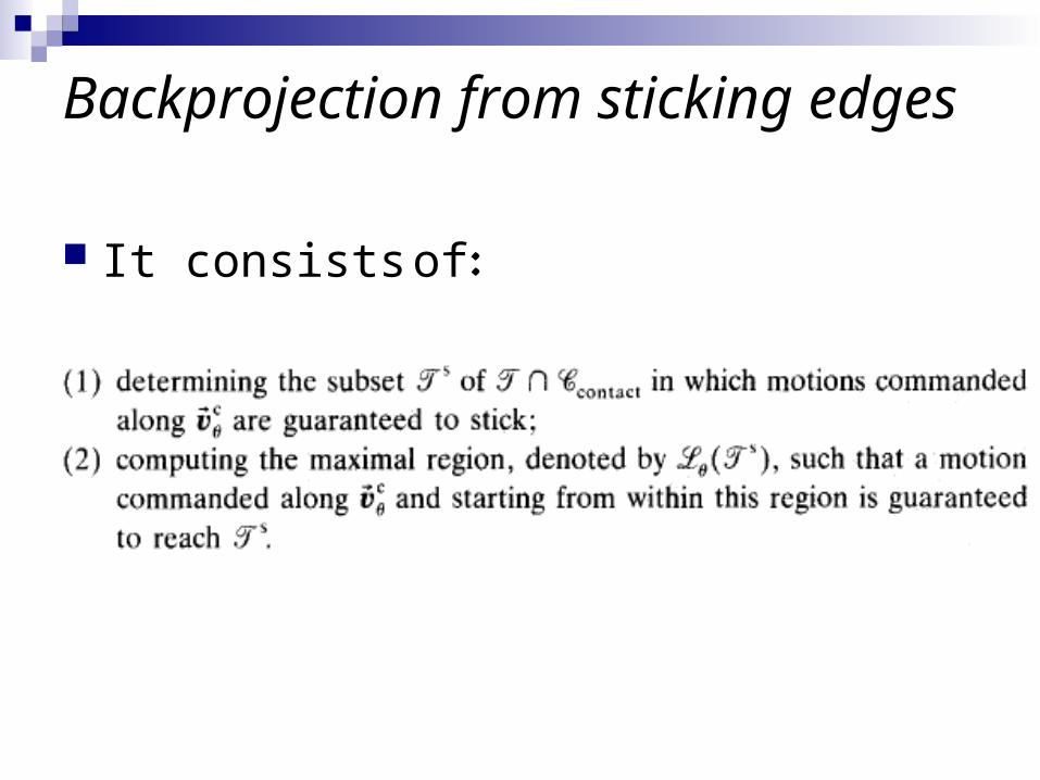
Backprojection from sticking edges

It consists of:

Backprojection from sticking edges

The region L (Js) is called the backprojection of Jsfor v1.

Erdmann gave a simple algorithm to compute the maximal backprojection of a single contact edge.

Step 1

Consider every vertex in Ccontact Mark every non-goal vertex at which sticking is possible. Mark every goal vertex if sliding away from the vertex in the non-goal edge is possible.

Step 2

At every marked vertex erect two rays parallel to the sides of the inverted control uncertainty cone. Compute the intersection of these rays among themselves and with Ccontact . Ignore each ray beyond the first intersection. The remaining segment in each ray is called a free edge.

Step 3

Trace out the backprojection region. To that purpose, trace the edge L in the direction that leaves the C-obstacle region on the right-hand side, until an endpoint is attained; then, let all the contact and free edges incident at this point be sorted clockwise in a circular list; trace the first edge following L in this list.

An Example

PreImage backchaining is a very general approach, however, raises difficult computational issues which still prevent its widespread application.

On solution is using Landmarks in the workspae.

Introduction of Landmark A typical notion for planning with uncertainty is

that of a landmark, an element of the workspace that can be detected reliably.

Sometimes, a direct path to the goal may seem attractive, but if it does not allow enough landmarks to be detected along the way, the robot may fail to attain the goal due to the errors in its planning models.

Introduction of Landmark

The overall task of the planner is:select an adequate set of states.associate appropriate motion commands

with these states. synthesize state recognition functions.

All three subtasks are interdependent.

The Concept of a landmark

Landmark : an “island of perfection” in the robot conguration space where position sensing and motion control are accurate.

However neither control nor sensing need be perfect in landmark regions.

It mainly reduces planning to selecting motion commands to navigate from landmark to landmark.

Similar notions for Landmark Similar notions have been previously introduced

as landmarks in the literature with dierent names :

atomic regions Signature neighborhoods perceptual equivalent classes sensory uncertainty field visual constraints

Creating landmarks

Creating landmarks requires some prior engineering of the robot and its environment.

It is important that its cost be reduced as much as possible.

Assumptions

The robot is a point moving in a plane. Obstacles are considered as circular regions. landmark disks are circular regions too. Both the obstacles and the landmark disks are

stationary. The number of landmark disks is finite(l) The number of obstacle disks is also finite(O(l)). We can consider l as a criteria for measuring the size

of the input problem.

Assumptions

The robot has perfect position sensing in the landmark disks and no sensing outside the landmark disks.

The direction of motion at any instant differs from the commanded direction of motion by an angle bounded by .

In the imperfect control mode the actual value of teta can be controllable by the robot in a connected interval

A motion command in the imperfect control mode is specied as a tripletd (d, ,L)

L is a set of landmark disks defning the termination condition.

The direction of motion at any instant differs from the commanded direction of motion by an angle bounded by teta.

Example 1

Assume a constant directional uncertainty is given.

The workspace contains 23 landmark disks shown white or grey forming 19 landmark regions and 25 obstacle disks

The white disks are those with which the planner has associated imperfect control motion commands to attain another landmark disk.

The algorithm

The algorithm assumes given constant directional uncertainty(0.09 radian).

It produces plans minimizing the number of motion commands to be executed.

The arrow attached to the initial region or a whitedisk is the commanded direction of a command

Example 2

Assuming controllable directional uncertainty.

The directional uncertainty is controllable in the interval [0.1 0.5].

The planner produces a one-step plan, a plan containing a single imperfect control motion command (d , , L)

extension of the goal

If a connected set of landmark disks intersects the goal region the robot can move into the goal from any point in this set.

The union of the landmark regions intersecting the goal is called the extension of the goal the other landmark disks are called the intermediate.

If the goal does not intersect any landmark disk then it is considered unachievabl.

zero step plan

Given a goal G we first compute its extension E(G).

If the initial region I lies entirely in E(G) no further planning effort is needed.

Indeed in a landmark region a plan is simply a geometric path whose computation is straightforward Such a plan is called a zero step plan.

one-step plan

If there does not exist a zerostep plan to achieve G the planner may try to find a pair (d, ) such that the initial region I is contained in the backprojection of E(G) for (d, ).

We call this plan a one-step plan.

A one step plan may not exist or may not be desirable if its cost is too high

Then the planner can attempt to create a multi-step plan iteratively.

The backprojection of the new goal extensions are computed.

Building the Discrete Search Space

Each planning iteration requires selecting a pair (d ) such that the backprojection of the current goal extension either contains the initial region I or intersects intermediategoal disks.

The d -space can be partitioned into an arrangement of curves defining cells.

The concept of cells

Each cell is regular in the following sense: The backprojection of the goal extension

for any pair (d, ) in a cell C contains the same initial position disks and intersects the same intermediategoal disks as the backprojection for any other pair (d’, ’) in C.

The number of cells is polynomial in the number of landmark and obstacle disks

Creation the arrangement of cells

Let us assume that no landmark disk intersects an obstacle disk.

The arrangement of cells is created by a network of curves corresponding to the some critical events.

I-cover event

An example of a critical point: I-cover event: A left ray of the

backprojection is tangent to an initial region disk with this disk on its righthand

sideLet s be the slope of the left ray tangent to the initial position disk.

The equation of the curve denoted by this event is :

There are eleven critical point and eleven corresponding equation.

Allowing landmark disks to intersect with obstacle disks would simply require con- sidering additional critical events It would not change the asymptotic complexity of the cell arrangement.

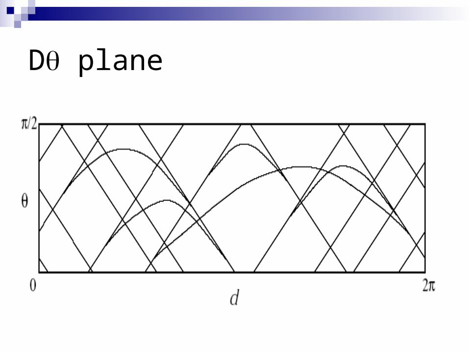
D plane

References

Jean-Claude Latombe, Anthony Lazanas and Shashank Shekhar, “Robot motion planning with uncertainty in sensing and control.

Anthony Lazanas, and Jean-Claude Latombe, “Motion Planning with Uncertainty:A Landmark Approach”

Thanks