Quantile Regression

Presented by

Dr. Neil W. Polhemus

Quantile Regression

• Constructs linear models for predicting specified quantiles.

• Useful when:

– primary interest concerns a percentile of the distribution rather than the mean.

– the distribution of the data at a specified combination of the predictor variables is not Gaussian.

– the variance of Y depends on X.

– there are outliers present.

Applications

• Growth curves

• Ecology

• Epidemiology

• Health services utilization

• CEO pay

• Household income

• Home prices

• Sea ice extent

• Astrophysics

• Chemistry

• Genomics

• Waiting times

• Product reliability

Basic Model Structure

Qt(Y): conditional t-th quantile of dependent

variable Y

X1, X2, … Xp: predictor variables

Note that the coefficients depend on t.

𝑄𝜏 𝑌 = 𝛽0 𝜏 + 𝛽1 𝜏 𝑋1 + 𝛽2 𝜏 𝑋2 +⋯+ 𝛽𝑝 𝜏 𝑋𝑝 + 𝜖

Statgraphics

• Statgraphics uses the quantreg program in R to fit

models.

• Quantreg was written by R. Koenker.

• You should download the latest build (19.2.02)

which includes a few tweaks to the Quantile

Regression procedure.

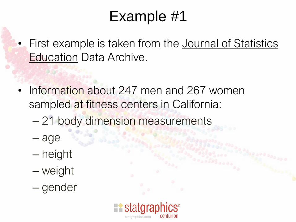
Example #1

• First example is taken from the Journal of Statistics

Education Data Archive.

• Information about 247 men and 267 women

sampled at fitness centers in California:

– 21 body dimension measurements

– age

– height

– weight

– gender

Histogram of Weight

males

females

80 120 160 200 240 280

60

40

20

0

20

40

60fr

eq

uen

cy

Box and Whisker Plot of Weight

Box-and-Whisker Plot

90 120 150 180 210 240 270

Weight

females

males

Comparison of Regression Lines

Genderfemalemale

Plot of Fitted Model

58 62 66 70 74 78

Height

90

120

150

180

210

240

270

Weig

ht

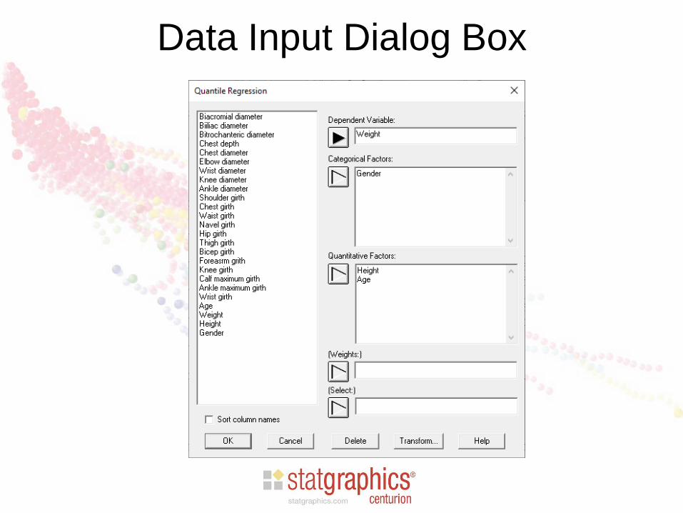
Data Input Dialog Box

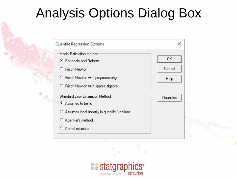
Analysis Options Dialog Box

Methods

• Barrodale and Roberts – for up to several

thousand observations.

• Frisch-Newton – useful for larger problems.

• Frisch-Newton with preprocessing – useful for

even larger problems. Best for large n and small p.

• Frisch-Newton with sparse algebra – useful for

large n and large p.

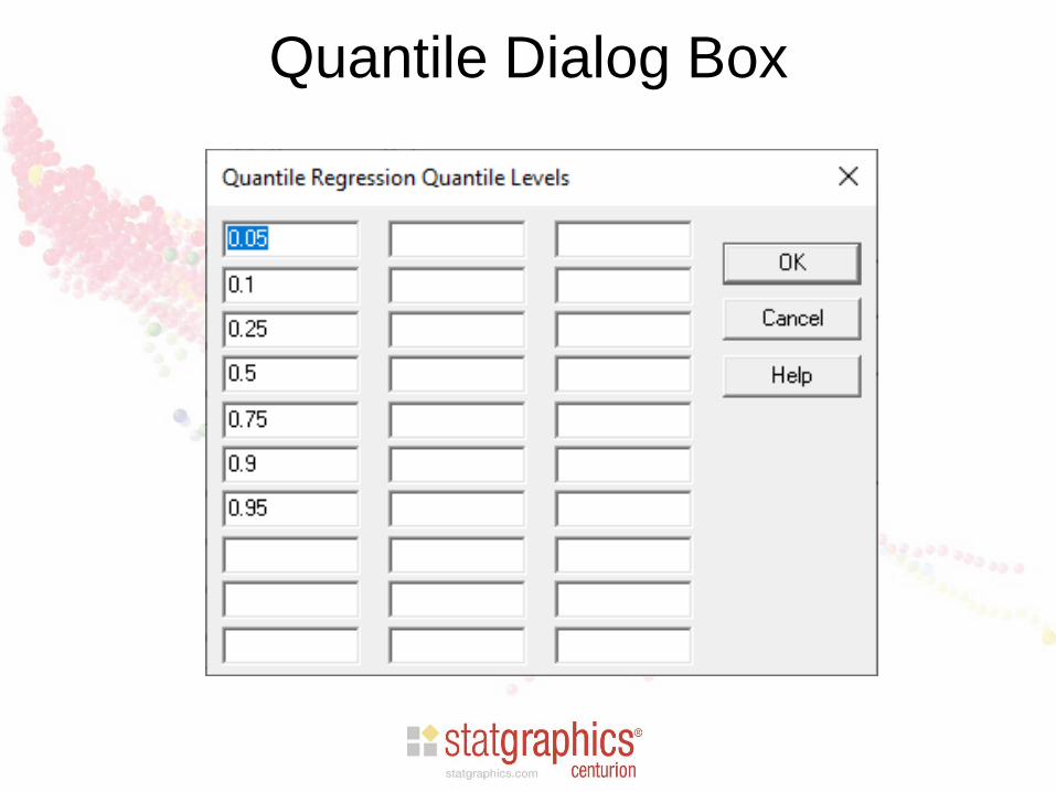
Quantile Dialog Box

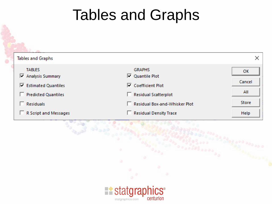
Tables and Graphs

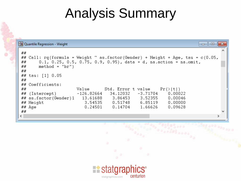
Analysis Summary

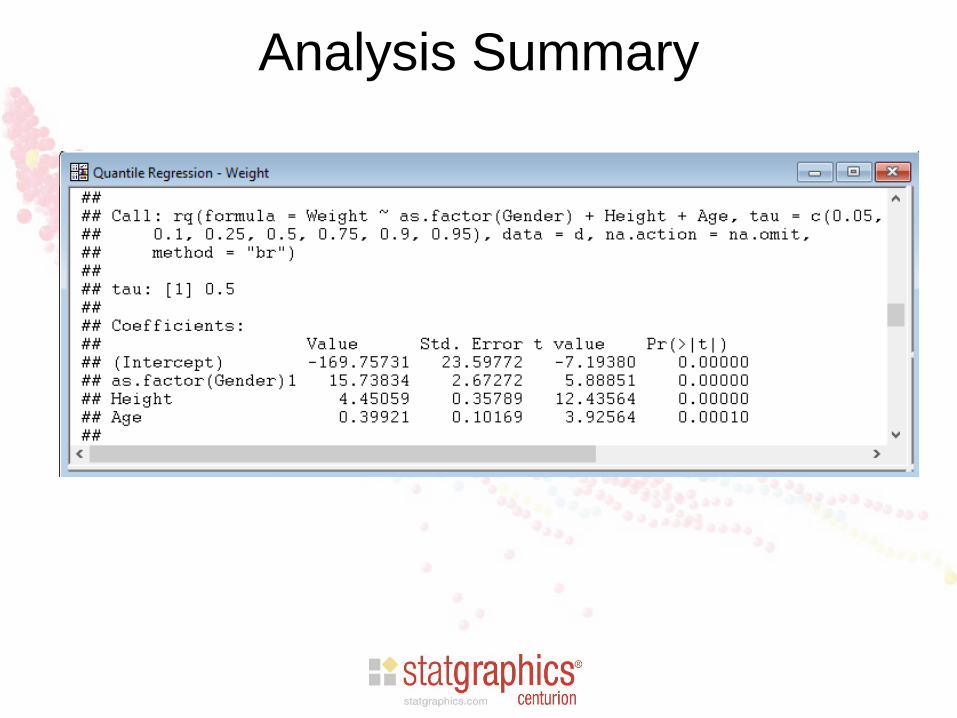
Analysis Summary

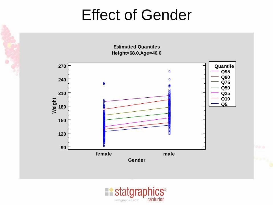
Effect of Gender

Estimated Quantiles

Height=68.0,Age=40.0

female male

Gender

90

120

150

180

210

240

270

Weig

ht

QuantileQ95Q90Q75Q50Q25Q10Q5

Effect of Height

Estimated Quantiles

Gender=1,Age=40.0

58 62 66 70 74 78

Height

90

120

150

180

210

240

270

Weig

ht

QuantileQ95Q90Q75Q50Q25Q10Q5

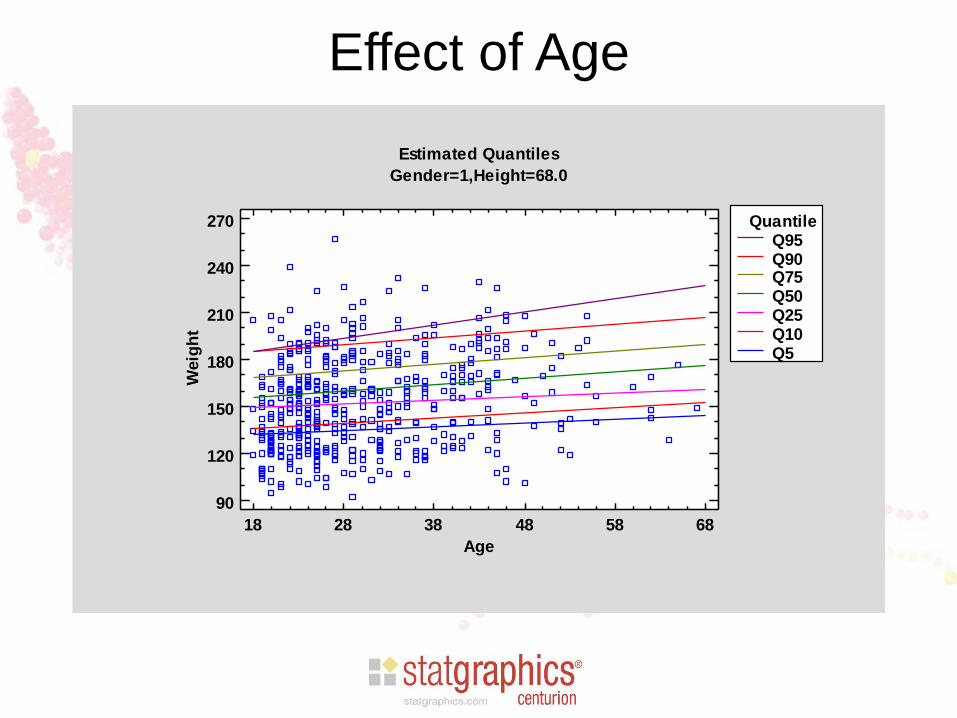
Effect of Age

Estimated Quantiles

Gender=1,Height=68.0

18 28 38 48 58 68

Age

90

120

150

180

210

240

270

Weig

ht

QuantileQ95Q90Q75Q50Q25Q10Q5

Estimated Quantiles

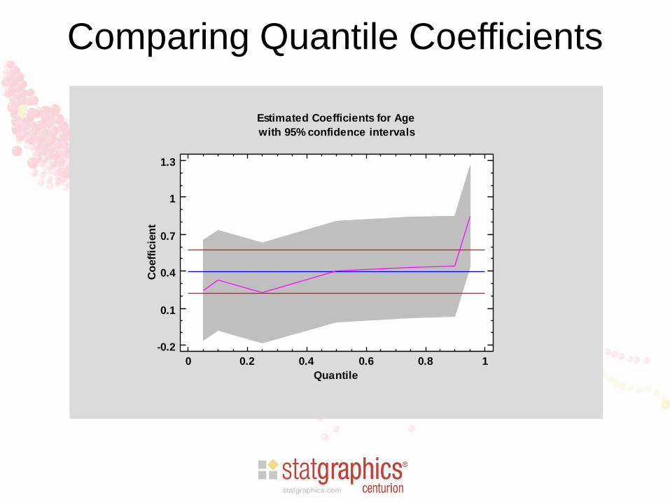
Comparing Quantile Coefficients

Estimated Coefficients for Age

with 95% confidence intervals

0 0.2 0.4 0.6 0.8 1

Quantile

-0.2

0.1

0.4

0.7

1

1.3C

oeff

icie

nt

Example #2

• Second example is also taken from the Journal of

Statistics Education Data Archive.

• Information about 93 makes and models of

automobiles manufactured in 1993

– Price of automobile

– Weight

Scatterplot

1600 2100 2600 3100 3600 4100 4600

Weight

0

20

40

60

80

Mid

Pri

ce

Plot of Mid Price vs Weight

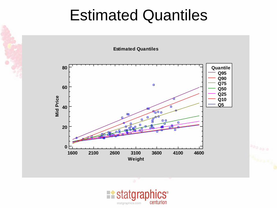
Estimated Quantiles

Estimated Quantiles

1600 2100 2600 3100 3600 4100 4600

Weight

0

20

40

60

80

Mid

Pri

ce

QuantileQ95Q90Q75Q50Q25Q10Q5

Comparing Quantile Coefficients

Estimated Coefficients for Weight

with 95% confidence intervals

0 0.2 0.4 0.6 0.8 1

Quantile

-4

6

16

26

36(X 0.001)

Co

eff

icie

nt

References

• StatFolios and data files are at: www.statgraphics.com/webinars

• R Package “quantreg” (2021) https://cran.r-project.org/web/packages/quantreg/quantreg.pdf

• Quantile Regression (2005) Roger Koenker. (Econometric Society Monographs, Series Number 38)

• Body and car data from: http://jse.amstat.org/jse_data_archive.htm