Presentazione di PowerPoint - Politecnico di...

Prof. Luca Bascetta ([email protected])

Politecnico di Milano

Dipartimento di Elettronica, Informazione e Bioingegneria

Automatic ControlMotion planning

mailto:[email protected]

Prof. Luca BascettaProf. Luca Bascetta

Motivations

Electric motors are used in many different applications, ranging from

machine tools and industrial robots to household appliances and advanced

driver assistance systems.

The motion of these motors should be appropriately controlled, starting from

the trajectory performed by the rotor.

A trajectory can be characterized by different profiles and maximum values

of velocity, acceleration and jerk, generating different effects on the

actuator, on the motion transmission system and on the mechanical load

performance and wear.

Motion planning is the activity aiming at selecting suitable velocity,

acceleration and jerk profiles.

2


Profile selection criteria

Which are the guidelines to select the profile?

• low computational complexity and memory consumption

• continuity of position, velocity (and jerk) profiles

• minimize undesired effects (curvature regularity)

• accuracy (no overshoot)

We will consider two different problems:

• point-to-point motion planning

only start and goal, and motion duration are specified

• trajectory planning

a set of desired positions is specified

3


Polynomial trajectories (I)

Let’s consider the point-to-point motion planning problem.

Given the initial and final conditions on position, velocity, acceleration and

jerk, and the motion duration, the easiest solution to the planning problem is

given by polynomial functions

The coefficients can be determined imposing the initial and final conditions.

Increasing the order of the polynomial, the trajectory becomes smoother

and we can satisfy more initial and final conditions.

We will now consider two classical examples: 3rd and 5th order polynomials.

4


Polynomial trajectories (II)

Given the following initial and final conditions:

• initial and final time (𝑡𝑖 and 𝑡𝑓)

• initial position and velocity (𝑞𝑖 and ሶ𝑞𝑖)

• final position and velocity (𝑞𝑓 and ሶ𝑞𝑓)

To satisfy the four boundary conditions we need at least a 3rd order

polynomial

Then, imposing the boundary conditions

we obtain (𝑇 = 𝑡𝑓 − 𝑡𝑖)

5


Polynomial trajectories – Example 6


Polynomial trajectories (III)

In order to enforce initial conditions on the acceleration as well, we need at

least a 5th order polynomial

Then, imposing the boundary conditions

we obtain (𝑇 = 𝑡𝑓 − 𝑡𝑖)

7


Polynomial trajectories (IV)

An harmonic motion is characterized by an acceleration profile that is

proportional to the position profile, with opposite sign.

A generalization of the harmonic trajectory is given by

where

Note that the harmonic trajectory has continuous derivatives (of any order)

∀𝑡 ∈ 𝑡𝑖, 𝑡𝑓 .

9


Polynomial trajectories (V)

In order to avoid discontinuities at 𝑡𝑖 and 𝑡𝑓 in the acceleration profile, we

can modify the harmonic trajectory introducing the cycloidal trajectory

where

11


Trapezoidal trajectories (I)

A very common way to plan the motion of a motor in industrial drives is

based on trapezoidal velocity profiles.

The trajectory is composed of a linear part, where the velocity is constant,

and two parabolic blends, where the velocity is a linear function of time.

The trajectory can be thus divided in three parts:

1. in the first part a constant acceleration is applied, the velocity is linear

and the position a parabolic function of time

2. in the second part the acceleration is zero, the velocity is constant and

the position is a linear function of time

3. in the third part a constant negative

acceleration is applied, the velocity is

linear and the position a parabolic

function of time

If 𝑇𝑎 = 𝑇𝑑 (𝑇𝑎 ≤ Τ(𝑡𝑓−𝑡𝑖) 2) the profile is

symmetric.

13


Trapezoidal trajectories (II) 14

First part (acceleration)

Second part (constant velocity)

Third part (deceleration)


Trapezoidal trajectories – Example 15


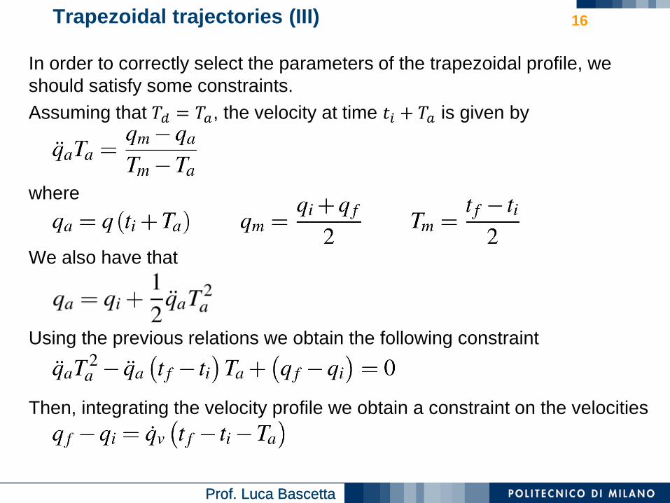
Trapezoidal trajectories (III)

In order to correctly select the parameters of the trapezoidal profile, we

should satisfy some constraints.

Assuming that 𝑇𝑑 = 𝑇𝑎, the velocity at time 𝑡𝑖 + 𝑇𝑎 is given by

where

We also have that

Using the previous relations we obtain the following constraint

Then, integrating the velocity profile we obtain a constraint on the velocities

16


Trapezoidal trajectories (IV)

Given

• the distance ℎ = 𝑞𝑓 − 𝑞𝑖

• the duration 𝑇 = 𝑡𝑓 − 𝑡𝑖

We have three different ways to specify the trajectory:

1. choosing the acceleration time 𝑇𝑎 (𝑇𝑎 < Τ𝑇 2)

2. choosing the acceleration ( ሷ𝑞𝑎 ≥ Τ4 ℎ 𝑇2)

3. choosing the velocity ( ሶ𝑞𝑣 ≥ Τℎ 𝑇)

17


Trapezoidal trajectories (V)

If we would like to select the maximum velocity and acceleration according

to the motor specifications, we have to select

• acceleration time 𝑇𝑎 =ሶ𝑞𝑚𝑎𝑥

ሷ𝑞𝑚𝑎𝑥

• distance ℎ = ሶ𝑞𝑚𝑎𝑥 𝑇 − 𝑇𝑎

In this case the duration will be

and the trajectory is described by the following equations

These equations hold only if 𝑇𝑎 ≤ Τ𝑇 2, or equivalently ℎ ≥ Τሶ𝑞𝑚𝑎𝑥2 ሷ𝑞𝑚𝑎𝑥.

18


Trapezoidal trajectories (VI)

If ℎ < Τሶ𝑞𝑚𝑎𝑥2 ሷ𝑞𝑚𝑎𝑥 the trajectory will not reach the maximum velocity and the

maximum acceleration.

If we would like to minimize the trajectory duration we can use a bang-bang

acceleration profile

where the acceleration time and the trajectory duration are

and the maximum velocity is

19


Trapezoidal trajectories (VII)

The trapezoidal velocity profile is characterized by a discontinuous

acceleration profile. As a consequence, jerk has infinite values in the

acceleration discontinuities.

This can negatively affect a mechanical system, increasing wear and

causing vibrations.

To overcome this problem we can introduce a continuous trapezoidal

acceleration profile.

The trajectory can be divided in three parts:

1. acceleration (acceleration

linearly increases until the

maximum value and then

linearly decreases)

2. constant velocity

3. deceleration (is symmetric to

phase 1)

20


Trajectory scaling (I)

Sometimes a planned trajectory need to be scaled in order to adapt to

actuator constraints.

There are two different solutions to this problem:

1. kinematic scaling, trajectory has to satisfy maximum acceleration and

maximum velocity constraints

2. dynamic scaling, trajectory has to satisfy maximum torque constraints

We will now consider the problem of kinematic scaling.

In order to scale a trajectory we need to parametrize it introducing a

normalized parameter 𝜎 = 𝜎 𝑡 .

Given a trajectory 𝑞 𝑡 , from 𝑞𝑖 to 𝑞𝑓, whose duration is 𝑇 = 𝑡𝑓 − 𝑡𝑖, the

normalized form is

where ℎ = 𝑞𝑓 − 𝑞𝑖 and

21


Trajectory scaling (II)

Considering the normalized form

we have

The maximum velocity, acceleration, … values correspond to the maximum

values of functions 𝜎 𝑖 𝜏 .

Modifying the trajectory duration 𝑇 one can satisfy the kinematic constraints.

22


Trajectory scaling (III)

Consider a 3rd order polynomial trajectory, we can introduce the parameter

Imposing the boundary conditions

we obtain

and consequently

Maximum velocity and acceleration are given by

23


Trajectory scaling (IV)

Consider a 5th order polynomial trajectory, we can introduce the parameter

Imposing the boundary conditions

we obtain

and consequently

Maximum velocity, acceleration and jerk are given by

24


Trajectory scaling (V)

A harmonic trajectory can be parameterized introducing

consequently


25


Trajectory scaling (VI)

A cycloidal trajectory can be parameterized introducing

consequently


26


Trajectory scaling – Example

Consider a trajectory with 𝑞𝑖 = 10°, 𝑞𝑓 = 50°, and a motor characterized by

ሶ𝑞𝑚𝑎𝑥 = 30 Τ° 𝑠 and ሷ𝑞𝑚𝑎𝑥 = 80 Τ° 𝑠2.

27

Trajectory Max vel/acc Constraints Min duration

3rd deg. poly 2

5th deg. poly 2.5

Harmonic 2.094

Cycloidal 2.667

Faster

Faster


Interpolation (I)

Up to now we have considered only point-to-point trajectories. In many

practical problems, however, we would like to determine a trajectory that

goes through multiple points.

This problem can be addressed using interpolation techniques.

We are now interested to determine a trajectory that goes through a set of

points at certain time instants

28


Interpolation (II)

To determine a trajectory that goes through 𝑛 points we can consider a

polynomial function of order 𝑛 − 1

Given a set of points 𝑡𝑖, 𝑞𝑖 𝑖 = 1,… , 𝑛, we can define vectors 𝐪 and 𝐚, and

Vandermonde matrix 𝐓 as follows

as a consequence

Caveat: matrix 𝑇 is always invertible if 𝑡𝑖 > 𝑡𝑖−1 𝑖 = 1,… , 𝑛.

29


Interpolation – Example

Polynomial interpolation with 4th order polynomial

30

𝒕𝒊 0 2 4 8 10

𝒒𝒊 10 20 0 30 40


Interpolation (III)

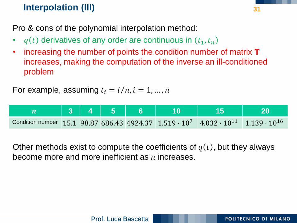
Pro & cons of the polynomial interpolation method:

• 𝑞 𝑡 derivatives of any order are continuous in 𝑡1, 𝑡𝑛• increasing the number of points the condition number of matrix 𝐓

increases, making the computation of the inverse an ill-conditioned

problem

For example, assuming 𝑡𝑖 = Τ𝑖 𝑛, 𝑖 = 1,… , 𝑛

Other methods exist to compute the coefficients of 𝑞 𝑡 , but they always

become more and more inefficient as 𝑛 increases.

31

𝒏 3 4 5 6 10 15 20

Condition number 15.1 98.87 686.43 4924.37 1.519 ⋅ 107 4.032 ⋅ 1011 1.139 ⋅ 1016


Interpolation (IV)

Other issues of polynomial interpolation are:

• the computational complexity of determining the coefficients increases as

𝑛 increases

• if a single point 𝑡𝑖 , 𝑞𝑖 changes we need to recompute all the coefficients

• if we add a point at the end of the trajectory 𝑡𝑛+1, 𝑞𝑛+1 we need to

increase the order of the polynomial and recompute all the coefficients

• the trajectory obtained with polynomial interpolation is usually affected by

undesired oscillations

In order to overcome these issues we can consider 𝑛 − 1 polynomials of

order 𝑝 (instead of just one polynomial), each one interpolating a segment

of the trajectory.

A first solution can be obtained using 3rd order polynomials and imposing

position and velocity constraints for each point of the trajectory, in order to

compute the cubic polynomial between two consecutive points.

32


Interpolation – Example 33

Polynomial interpolation with 3rd order polynomial segments

𝒕𝒊 0 2 4 8 10

𝒒𝒊 10 20 0 30 40

ሶ𝒒𝒊 0/s -10/s 10/s 3/s 0/s


Interpolation (V)

If only the desired points are specified, we can compute the velocities using

the following relations

where

is the slope between points at 𝑡𝑘−1 and 𝑡𝑘.

34



Polynomial interpolation with 3rd order polynomial segments

𝒕𝒊 0 2 4 8 10

𝒒𝒊 10 20 0 30 40


Interpolation (VI)

As you have seen in the example, a trajectory generated with cubic

interpolation is affected by discontinuities in the acceleration.

To overcome this problem we can still use cubic segments, but we should

specify only the position of each point and impose the continuity of position,

velocity and acceleration.

This approach leads to the so called smooth path line (spline).

Among all the interpolating functions ensuring continuity of the derivatives,

the spline is the one that has minimum curvature.

Let’s study now how to determine the coefficients of the cubic segments that

form the spline.

36


Interpolation (VII)

If we consider 𝑛 points we will have 𝑛 − 1 cubic polynomials

each one characterized by 4 coefficients. We have thus to determine

4 𝑛 − 1 coefficients, imposing the following constraints:

• 2 𝑛 − 1 interpolation conditions (every cubic segment should start and

end in a trajectory point)

• 𝑛 − 2 continuity conditions on the velocity of the inner points

• 𝑛 − 2 continuity conditions on the accelerations of the inner points

At the end we have 4 𝑛 − 1 coefficients and only 4𝑛 − 6 constraints.

We can enforce two more constraints imposing, for example, the initial and

final velocity.

Let’s summarize the problem.

37


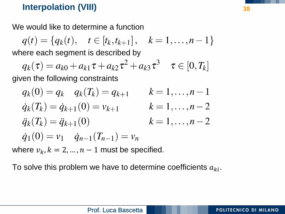
Interpolation (VIII)

We would like to determine a function

where each segment is described by

given the following constraints

where 𝑣𝑘 , 𝑘 = 2, … , 𝑛 − 1 must be specified.

To solve this problem we have to determine coefficients 𝑎𝑘𝑖.

38


Interpolation (IX)

We start assuming velocities 𝑣𝑘 , 𝑘 = 2,… , 𝑛 − 1 known.

For each cubic polynomial we have 4 boundary conditions on positions and

velocities, giving rise to the following system

Solving this system with respect to the coefficients yields

39


Interpolation (X)

In order to compute velocities 𝑣𝑘 , 𝑘 = 2,… , 𝑛 − 1 we impose 𝑛 continuity

conditions on the accelerations of the intermediate points

If we now substitute the expressions of coefficients 𝑎𝑘2, 𝑎𝑘3, 𝑎𝑘+1,2, and

multiply by Τ𝑇𝑘𝑇𝑘+1 2, we obtain

and in matrix form

where 𝑐𝑘 are functions of the intermediate positions and the duration of

each segment.

40


Interpolation (XI)

Finally, neglecting 𝑣1 and 𝑣𝑛 that are known, we have

This is a set of 𝑛 − 2 linear equations that can be written as 𝐀𝐯 = 𝐜.

41


Interpolation (XII)

We observe that

• matrix 𝐀 is a diagonally dominant matrix, and is always invertible for 𝑇𝑘 >0

• matrix 𝐀 is a tridiagonal matrix, implying that numerically efficient

techniques exist (Gauss-Jordan method) to compute its inverse

• once the inverse of matrix 𝐀 is known, we can compute velocities

𝑣2, … , 𝑣𝑛−1 as follows

We can derive a similar procedure to determine the spline using the

intermediate accelerations instead of the intermediate velocities.

42


Interpolation (XIII)

We conclude observing that the total duration of the trajectory is given by

In many applications one is interested to find the minimum time trajectory.

This goal can be achieved determining the segment durations 𝑇𝑘 that

minimize 𝑇, satisfying the maximum velocity and maximum acceleration

constraints:

This is a nonlinear optimization problem with linear cost function.

43



Cubic spline interpolation

𝒕𝒊 0 2 4 8 10

𝒒𝒊 10 20 0 30 40

Presentazione di PowerPoint - Politecnico di...

Documents

Transcript of Presentazione di PowerPoint - Politecnico di...