Presentation v3.2

INNOVATIVE METHODS FOR THE RECONSTRUCTION

OF NEW GENERATION SATELLITE REMOTE SENSING

IMAGES

November 29th, 2012

PhD Student: Luca Lorenzi

[email protected]

Ph.D. thesis defense

Advisors: Farid Melgani

Grégoire Mercier

Introduction – General Problem

Missing data in VHR optical image;

Mainly due to acquisition conditions, e.g., the presence of:

clouds: partially or completely missing data;

shadows: partially missing data.

2

MODIS: Black see

GeoEye-1: Doha Stadium, Qatar

Introduction – General Solution

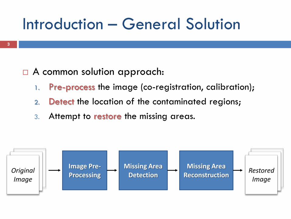
A common solution approach:

1. Pre-process the image (co-registration, calibration);

2. Detect the location of the contaminated regions;

3. Attempt to restore the missing areas.

3

Missing Area Detection

Missing Area Reconstruction

Original Image

Image Pre-Processing

Restored Image

Objective

Propose new methodologies for the reconstruction of

missing areas for new generation satellite remote

sensing images.

Missing areas due to the presence of:

Clouds

Shadows

4

Cloud-Contaminated Images

Contribution 1: different solutions based on the inpainting approach.

Three strategies:

local image properties;

isometric transformations;

multiresolution processing scheme.

Contribution 2: to improve the reconstruction process by integrating both

radiometric and spatial information, through a specific kernel.

Contribution 3: new methods based on the Compressive Sensing theory.

Three strategies:

Orthogonal Matching Pursuit (OMP);

Basis Pursuit (BP);

An alternative solution based on Genetic Algorithms (GAs).

5

Shadow-Contaminated Images

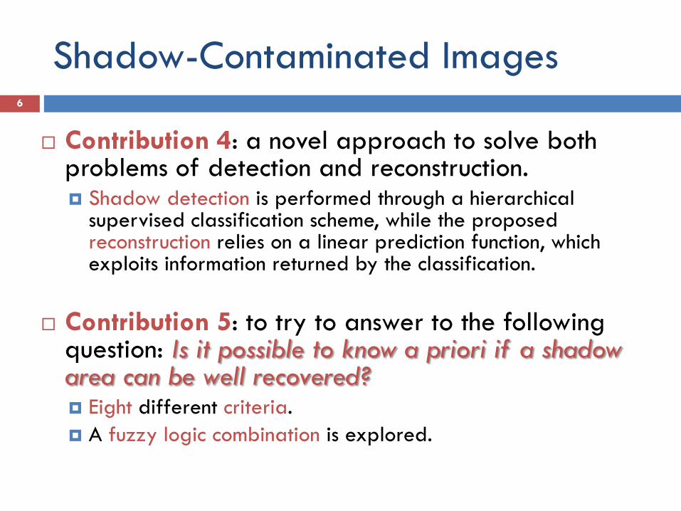
Contribution 4: a novel approach to solve both problems of detection and reconstruction. Shadow detection is performed through a hierarchical

supervised classification scheme, while the proposed reconstruction relies on a linear prediction function, which exploits information returned by the classification.

Contribution 5: to try to answer to the following question: Is it possible to know a priori if a shadow area can be well recovered? Eight different criteria.

A fuzzy logic combination is explored.

6

… two contributions in detail

In the next Slides…

MISSING AREA RECONSTRUCTION IN

MULTISPECTRAL IMAGES UNDER A COMPRESSIVE

SENSING PERSPECTIVE

PUBLISHED IN THE IEEE TRANSACTIONS ON GEOSCIENCE AND REMOTE SENSING,

VOL. 51, IN PRESS, 2013

L. Lorenzi, F. Melgani, and G. Mercier

Problem formulation

In I(1), any pixel can be expressed as:

We have to evaluate:

From I(1) :

In I(2) :

9

2,1 ,)()()( iI iiiΦΩ

)1()1(Ωx

)1()1()1( , , ΩαΦ lkx

)1()1( , xf Φα

αΦ )2()2(x̂ f ?

source area

missing area

Compressive sensing (CS)

Compressive sensing theory [1]

Idea: exploit redundancy in signals

Signals like images are sparse → many coefficients close to zero

To enforce the sparsity constraint, CS finds a vector which minimizes:

D is a dictionary with a predefined number of atoms;

x is the original pixel, expressed by a linear combination of atoms;

Eq. (1) represents a NP-hard problem → computationally infeasible to

solve.

Candès and Tao [2], reduce the Eq. (1) in a relatively easy linear

programming solution:

under some reasonable assumptions:

10

αα Dx subject to min0

0:#0

ii α

(1)

[1] D. L. Donoho, “Compressed Sensing”, IEEE Trans. Inf. Theory, vol. 52, no. 4, pp. 1289-1306, Apr 2006.

[2] E. J. Candès and T. Tao, “Decoding by Linear Programming”, IEEE Trans. Inform. Theory, vol. 51, no. 12, pp. 4203-4215, Dec. 2005.

01minmin

Orthogonal Matching Pursuit (OMP) 12

[3] Y. C. Pati, R. Rezaiifar and P. S. Krishnaprasad, “Orthogonal Matching Pursuit: Recursive Function Approximation with Applications to

Wavelet Decompositions”, in Proc. 27th Asilomar Conf. on Sig., Sys. and Comp., Nov. 1-3, 1993.

Orthogonal Matching Pursuit (OMP) [3] finds the atoms

which has the highest correlation with the signal:

where dictionary D is a collection of atom vectors and R(m) is a

residual.

It updates the coefficients of the selected atoms at

each iteration (adopting a least-squares step), so that

the resulting residual vector R is orthogonal to the

subspace spanned by the selected atoms.

)(

1

mm

i

dd

Dd

dd Rxii

Ddd

Orthogonal Matching Pursuit (OMP) 13

OMP pseudo code

i=0: x(0)=0 , R(0)=x and D(c0)={∅}

i=k:

i=m: ,

)(

1

)( mm

i

dd

m Rxii

)(mRR

Step 1: find which ;

→ add to the set of selected variables;

→ update .

Step 2: let denote the projection onto the linear

space spanned by the elements of

→ update

Step 3: compute s.t.

Step 4: if ||R(k)||<th, stop, else set k=k+1 and return to Step 1

)1( max kT

jj

R

kj

kkk jcc 1

Tkk

T

kkk ccccP 1

icD

kj

xPIR k

k )(

)(kx

i

i

ci

d

k

i

kx )()(

1.

2.

3.

kk

k vAb 1)(

)1,...,1( )()()1()( kib k

i

k

k

k

i

k

i

k

i

jj

k

i

j

Tk

k

k

ki

k

b

R

1

)(

)(

)(

,1

Basis Pursuit (BP)

To solve Eq. (1), we may adopt the Basis Pursuit principle [4]: convexification from L0 to L1;

Thanks to that, it becomes a support minimization problem;

Eq. (2) can be reformulated as a linear programming (LP) problem, and solved using the Simplex methods.

Given that, it is possible to rewrite L1 norm in Eq. (2) as:

where

If we substitute it in Eq. (2), it allows to perform a linear minimization problem.

14

[4] S. S. Chen, D. L. Donoho and M. A. Saunders, “Atomic Decomposition by Basis Pursuit”, SIAM J. on Sci. Comp., vol. 20, pp. 33-61, 1999.


(2)

i iii i vu

1α

0 0 ,

0 0 ,

iiii

iiii

ifuv

ifvu

Genetic Algorithm (GA)

To cope with complex optimization problems, there exist metaheuristic techniques, like the evolutionary algorithms.

Genetic Algorithms (GAs) [5] are:

inspired by evolutionary biology;

general purpose randomized optimization techniques;

based on simple rules.

Their basic idea is to evolve iteratively a population of chromosomes, each representing a candidate solution to the considered problem.

In complex problems requiring the simultaneous optimization of multiple objectives, GAs are particularly indicated for they deal simultaneously with a population of solutions.

Advantages:

little information about the problem required;

robust to local optima;

optimization of real, integer and binary problems.

15

[5] L. Chambers, The Practical Handbook of Genetic Algorithms. New York: Champan & Hall, 2001.

GA – Principal Steps

1. Initial population of M chromosomes is generated;

2. The goodness of each chromosome is evaluated according to predefined fitness functions;

3. Successively, the GA favors the selection of the best chromosomes and removes the others;

4. In the next step a new population is represented by adopting genetic operators, e.g., crossover and mutation;

5. All these steps are iterated until a predefined condition is satisfied.

16

Condition

satisfied?

Ne

xt ite

ratio

n

Y

N

GA – Setup

Idea: exploit the GA capabilities for solving the L0 norm problem.

The NP-hard problem is:

Chromosome structure:

The number of chromosomes M must be fixed;

αi is a chromosome which contains w genes with real values;

The length w of the chromosome is thus equal to the one of the dictionary D.

17

Gene 1 Gene 2 Gene w

… i1 … i2 iw

Chromosome i

Fitness functions:

Multiple objective optimization [6] →

01 min αf

2

22 min xDf α

NSGA-2


(1)

[6] K. Deb, Multi-Objective Optimization Using Evolutionary Algorithms. Chichester, U.K.: Wiley, 2001.

Experimental Dataset

Aim: to compare the results obtained by the CS reconstructions with:

Multiresolution Inpainting (MRI) [7]

Contextual Multiple Linear Prediction (CMLP) [8]

In order to quantify the reconstruction accuracy:

1. consider I(1) cloud-free

2. simulate a presence of clouds by obscuring partly I(2)

3. compare the reconstructed I(2) with its original one

Evaluate the sensitivity to two aspects:

Test 1: kind of ground cover obscured

Test 2: size of the contaminated area

20

[7] L. Lorenzi, F. Melgani and G. Mercier, “Inpainting Strategies for Reconstruction of Missing Data in VHR Images”, IEEE Geosci. Remote Sens.

Letters, vol. 8, no. 5, pp. 914-918, Sep. 2011.

[8] F. Melgani, “Contextual Reconstruction of Cloud-Contaminated Multitemporal Multispectral Images”, IEEE Trans. Geosci. Remote Sens., vol. 44,

no. 2, pp. 442–455, Feb. 2006.

Multiresolution Inpainting (MRI)

Based on the Region-based inpainting (RBI) from Criminisi et al [9]

21

[7] L. Lorenzi, F. Melgani and G. Mercier, “Inpainting Strategies for Reconstruction of Missing Data in VHR Images”, IEEE Geosci. Remote Sens.

Letters, vol. 8, no. 5, pp. 914-918, Sep. 2011.

[9] A. Criminisi, P. Perez and K. Toyama, “Region filling and object removal by exemplar-based image inpainting”, IEEE Trans. on Image Process.,

vol. 13, no. 9, pp. 1-14, Sep 2004.

In [7], we proposed a processing scheme which

recursively injects multiresolution information for

a better reconstruction of the missing area.

Contextual Multiple Linear Prediction

Contextual Multiple Linear Prediction

(CMLP) [8] :

Training:

Prediction:

22

A simple solution is based on the

minimum square error pseudoinverse

technique.

[8] F. Melgani, “Contextual Reconstruction of Cloud-Contaminated Multitemporal Multispectral Images”, IEEE Trans. Geosci. Remote Sens., vol. 44, no. 2,

pp. 442–455, Feb. 2006.

Test 1

Contamination of Different Ground Cover

We suppose multiple land cover contamination, namely

different areas of the image are missing

Each mask is composed by ~2,000 pixels

23

Test 1

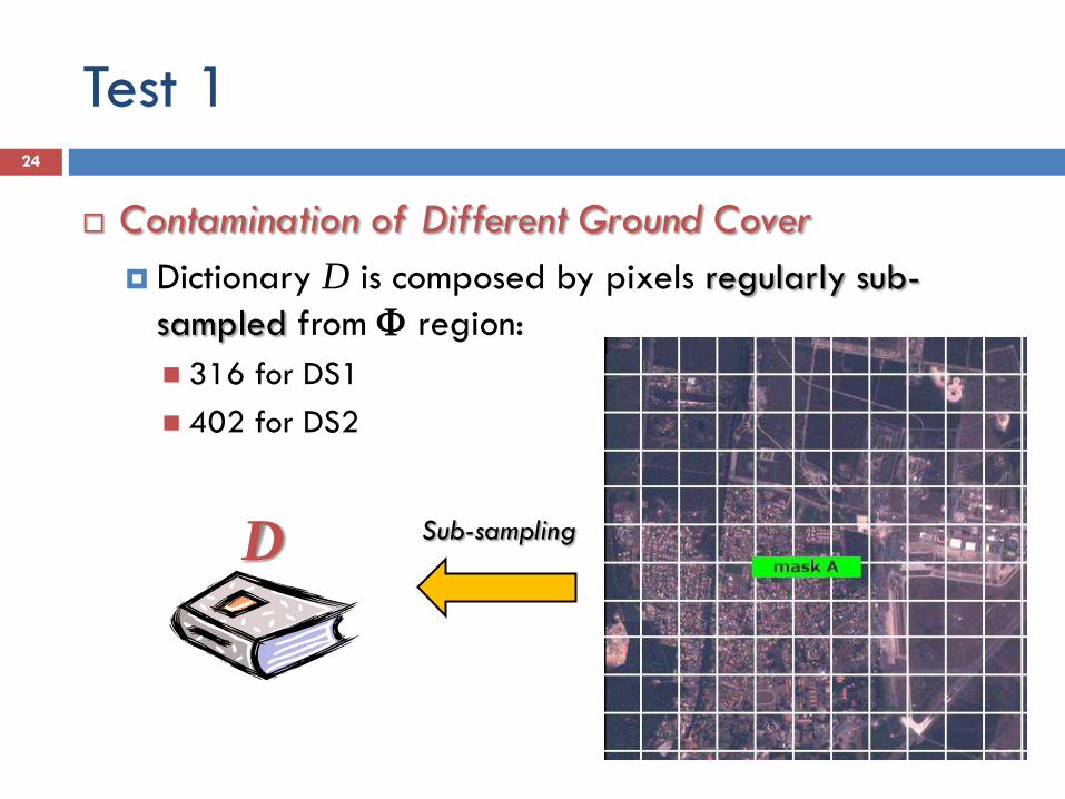
Contamination of Different Ground Cover

Dictionary D is composed by pixels regularly sub-

sampled from region:

316 for DS1

402 for DS2

24

D Sub-sampling

Test 1 – Datasets 1 & 2 26

Mask A Mask B Mask C

PSNR Complexity Time [s] PSNR Complexity Time [s] PSNR Complexity Time [s]

MRI 22.54 - 2856 16.05 - 2517 33.77 - 2898

CMLP 20.99 1 1 20.11 1 1 24.05 1 1

OMP 23.96 3 4 20.60 3 4 31.97 3 4

BP 22.22 294 66 24.74 168 59 30.67 301 60

GA 23.78 148 68621 23.15 95 26312 32.01 138 43193

Mask A Mask B

PSNR Complexity Time [s] PSNR Complexity Time [s]

MRI 24.27 - 2995 29.54 - 3614

CMLP 24.61 1 1 27.69 1 1

OMP 26.36 3 5 30.43 3 5

BP 26.45 338 61 31.63 365 91

GA 26.72 173 69231 31.28 201 38475

Dataset 1

Dataset 2

Test 1 – Dataset 1, Mask B 28

Reconstructed by OMP Reconstructed by BP Reconstructed by GA

Original crop of I(2) Reconstructed by MRI Reconstructed by CMLP

Test 2

Contamination with Different Sizes

We increase the amount of missing data:

mask 1: ~2,000 pixels



Dictionary D is composed as in Test 1

29

Test 2 – Datasets 1 & 2 30

Mask 1 Mask 2 Mask 3


MRI 22.54 - 2856 21.35 - 6938 19.63 - 14774

CMLP 20.99 1 1 21.13 1 1 20.83 1 2

OMP 23.96 3 4 23.21 7 6 25.01 3 19

BP 22.22 294 66 22.89 277 145 21.47 265 865

GA 23.78 148 68621 23.85 140 99072 23.03 149 275394

Mask 1 Mask 2 Mask 3


MRI 24.27 - 2995 22.85 - 10176 23.82 - 22353

CMLP 24.61 1 1 24.43 1 2 25.46 1 2

OMP 26.36 3 5 26.42 3 16 27.39 3 21

BP 26.45 338 61 26.82 332 143 28.25 329 972

GA 26.72 173 69231 27.10 168 103342 28.15 170 259459

Dataset 1

Dataset 2

Test 2 – Dataset 2, Mask 3 31

Reconstructed by OMP Reconstructed by BP Reconstructed by GA

Original crop of I(2) Reconstructed by MRI Reconstructed by CMLP

A COMPLETE PROCESSING CHAIN FOR

SHADOW DETECTION AND RECONSTRUCTION

IN VHR IMAGES

PUBLISHED IN THE IEEE TRANSACTION ON GEOSCIENCE AND REMOTE SENSING, VOL.

50, NO. 9, pp. 3440–3452, SEPTEMBER 2012

L. Lorenzi, F. Melgani, and G. Mercier

Introduction

In VHR optical images the presence of shadows partially obscures the scenario.

Missing information directly influences common processing and analysis operations (e.g. classification).

Shadows can be divided in two classes:

self shadow;

cast shadow.

Hypothesis: shadow and non-shadow classes follow a Gaussian distribution → more simple and more fast.

Denoting the shadow class as and the non-shadow class as , the reconstruction of the shadow class will be reduced to a simple random variable transformation:

33

2,~SS

NY

22 ,~ˆ,~SSSS NYNX

,~ 2

SSNX

General Block Diagram 34

Supervised

classification

of shadow areas

Original

Image

Restored

Image

Morphological

filtering

Shadow

reconstruction

Border

interpolation

Border

creation

Supervised

classification

of non-shadow

areas

Supervised

shadow vs

non-shadow

classification

I M1 M2 MF

C

Post-

classification &

quality control

Step1 - Binary Classification

Separate between shadow and non-shadow areas in the given image:

Supervised classifier: Support Vector Machine (SVM).

Human help: ROIs collection for Training set.

Feature space defined by:

original image spectral bands;

one-level stationary wavelet transform applied on each spectral band.

We adopt a Gaussian kernel:

35

Mask M1 Original image

2

2121 exp, xxxxKRBF

Step2 - Morphological filtering

It is usually adopted to eliminate “salt and pepper”

noise in the images.

We use an opening by reconstruction (erosion (ε)

followed by dilation (δ) ) followed by a closing by

reconstruction (dilation followed by erosion) to

obtain M2.

The size of the structuring element (SE) is 3x3

36

Mask M1 Mask M2

Step3 - Border Creation

The transition in-between shadow and non-shadow areas can raise problems:

e.g., boundary ambiguity, color inconstancy, and illumination variation.

Indeed, the presence of the penumbra induces mixed pixels which are difficult to classify.

We create a border also adopting morphological operators:

Note that the border is not needed in all directions, but only where we have the penumbra.

38

22 MMB

Mask M2 Mask MF

Step4 - Multiclass Classification

At this step, shadow and non-shadow areas are classified:

the previously mask MF is here exploited to guide the

classification;

note that the same ROIs are adopted here;

to improve map C, a 3x3 majority filter is adopted.

39

Mask MF

Original image Non-shadow classes

Shadow classes

Multiclass

classification

Map C Post-classification

map

Step5 - Quality Control

After the classification, both user (commission errors or inclusions) and producer (omission errors or exclusions) accuracies are derived (UA and PA).

UA: an error of commission results when a pixel is committed to an incorrect class;

PA: an error of omission results when a pixel is incorrectly classified into another category.

If one of these is lower than a predefined value (80%), it means that the classification of the corresponding thematic class is considered of low quality.

In such case, the related shadow compensation is not performed.

40

Step6 - Border Reconstruction

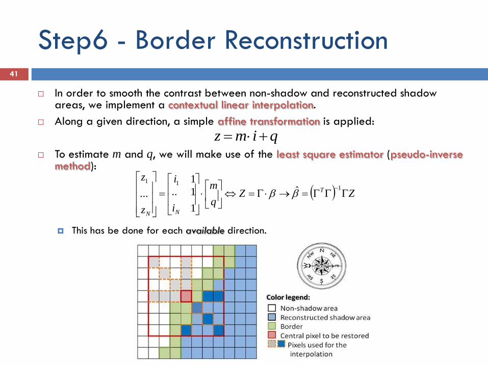
In order to smooth the contrast between non-shadow and reconstructed shadow areas, we implement a contextual linear interpolation.

Along a given direction, a simple affine transformation is applied:

To estimate m and q, we will make use of the least square estimator (pseudo-inverse method):

This has be done for each available direction.

41

qimz

ZZq

m

i

i

z

zT

NN

1

11

ˆ

1

1..

1

...

Dataset Description

Boumerdès (Algeria) Atlanta (USA) Jeddah (Saudi Arabia)

QuickBird

4 spectral bands

0.6 m of resolution

Acquired 28th Feb 2008

16% of shadow cover

IKONOS-2

3 spectral bands

1 m of resolution

Acquired 1998

42% of shadow cover

IKONOS-2

3 spectral bands

1 m of resolution

Acquired 11th Apr 2004

15% of shadow cover

42

Experimental Results-Binary classification

43

Experimental Results-Morphological Filtering

44

Experimental Results-Border creation

45

Experimental Results-Multiclass classification

46

Non-shadow classes Shadow classes

Experimental Results – Quality Check

The classification accuracies achieved on the test sets

Quality check: User’s and producer’s accuracies

if both are greater than 80% reconstruction

47

Non-shadow classes Shadow classes

Boumerdès 100 100 100 100 100 92 96 60

Atlanta 99 98 91 99 93 92 0 -

Jeddah 100 100 85 91 96 0 52 -

User’s accuracy Producer’s accuracy

Boumerdès 100 92 96 60 100 85 98 71

Atlanta 93 92 0 - 88 94 0 -

Jeddah 96 0 52 - 84 - 54 -

1S 2S 3S4S

1S 2S3S 4S

1S 2S 3S4S1S 2S 3S

4S

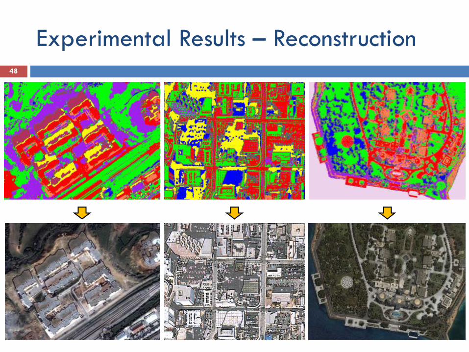
Experimental Results – Reconstruction 48

Experimental Results–Border Reconstruction

49

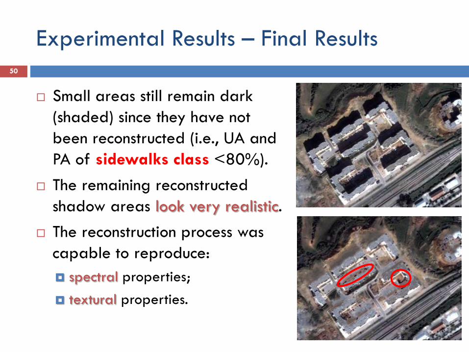
Experimental Results – Final Results

Small areas still remain dark

(shaded) since they have not

been reconstructed (i.e., UA and

PA of sidewalks class <80%).

The remaining reconstructed

shadow areas look very realistic.

The reconstruction process was

capable to reproduce:

spectral properties;

textural properties.

50


Here the results are more mitigated, mainly because of

the darkness and the heterogeneity of the shadow

regions.

Misclassification errors or false alarms, e.g.:

1. a dark roof of a building in the top of the image;

2. the self shadows of some buildings on the left

part of the image;

3. the shadow on the roof in the center of the

image.

Intrinsic complexity of some classes, e.g., the

asphalt class:

Both accuracies (UA and PA) are high, but the

reconstructed shadows appear noisy; the cause

seems to be the multimodal nature of this class.

However, some shadow regions are well reconstructed,

like the bright roofs in the bottom part of the image.

51


The Jeddah image is instead marked by a lot of thin shadows mostly located in vegetation areas.

The shadow thinness is explained by the steepness of the sun angle at the local image acquisition hour (11:17 a.m.).

Here the reconstruction, which was limited to the shaded vegetation, was globally satisfactory.

52

Impact on Classification Accuracy 54

76 95 74 0(*) 81 78 15(*) 58 0(*) 55(*)

Symbol (*) means that the shadow class was not reconstructed.

GENERAL CONCLUSIONS

Conclusion

In this presentation, missing data problems on very high spatial resolution (VHR) optical satellite have been investigated, in order to detect and/or reconstruct obscured areas. In particular, we face the problem of:

a complete obscuration due to the presence of cloudy areas;

partial contamination associated with shadow regions.

Inpainting strategies (contribution 1):

independent from the sensor type and from its spatial, temporal and spectral properties;

completely unsupervised;

sensitivity to the size of the missing area.

Regression with kernel combination (contribution 2):

the fusion of different types of information performed by means of a kernel combination have made the process particularly promising;

higher (but still contained) computation time.

59

Conclusion

Compressive sensing strategies (contribution 3):

good results in the reconstruction of missing areas;

they do not depend on the size of missing area;

completely unsupervised;

sensitivity to the kind of the missing area.

Shadow detection and compensation (contribution 4):

realistic shadow-free images with a promising preservation of spectral and textural properties;

in case of multimodal non-shadow classes, the implemented linear compensation method can be found inappropriate.

Shadow reconstructability (contribution 5):

angular second-moment difference, homogeneity difference and variance ratio behave better than the others;

fusing from 8 to 2 criteria, proved to be a useful way to capture the synergies between the different criteria;

subjective assessment of the reconstructability of shadow areas.

60

Future works

Since three years of research are never enough, future works about the problem of missing data can understandably be envisioned. For example:

regarding the inpainting, it could be interesting to integrate the temporal dimension in the process of reconstruction;

about the compressive sensing approach:

we think that it could be interesting to opt for smart techniques to design the dictionary, focusing on the context of the missing area;

another possible development is the addition of features in the training step of the CS (e.g., Haralick textures, Hu invariant moments, …);

regarding the shadow area reconstruction, we may envision to resort to nonlinear method in case linear regression does not work in a proper way.

In general, for each of the works presented here, it would be particularly interesting to reformulate or adapt it in view of an application for large-scale images knowing that such images raise the problem of spatial variance.

61

PUBLICATIONS

List of Related Publications

Journal papers

[J.1] L. Lorenzi, F. Melgani and G. Mercier, “Inpainting strategies for reconstruction of missing data in VHR images,” IEEE Geosci. Remote Sens. Lett., vol. 8, no. 6, pp. 914–918, Sep. 2011.

[J.2] L. Lorenzi, F. Melgani and G. Mercier, “A complete chain for shadow detection and reconstruction in VHR images,” IEEE Trans. Geosci. Remote Sens., vol. 50, no. 9, pp. 3440–3452, Sep. 2012.

[J.3] L. Lorenzi, F. Melgani and G. Mercier, “A support vector regression with kernel combination for missing data reconstruction,” IEEE Geosci. Remote Sens. Lett., in press.

[J.4] L. Lorenzi, F. Melgani, G. Mercier and Y. Bazi, “Assessing the reconstructability of shadow areas in VHR images,” IEEE Trans. Geosci. Remote Sens., in press.

[J.5] L. Lorenzi, F. Melgani and G. Mercier, “Missing area reconstruction in multispectral images under a compressive sensing perspective,” IEEE Trans. Geosci. Remote Sens., vol. 51, in press, 2013.

Conferences

[C.1] L. Lorenzi, F. Melgani and G. Mercier, “Multiresolution inpainting for reconstruction of missing data in VHR images,” in Proc. IGARSS, Vancouver, Canada, Jul. 2011.

[C.2] L. Lorenzi, F. Melgani and G. Mercier, “Orthogonal matching pursuit for VHR image reconstruction,” in Proc. IGARSS, Munich, Germany, Jul. 2012.

[C.3] L. Lorenzi, F. Melgani and G. Mercier, “Some criteria to assess the reconstructability of shadow areas,” in Proc. IGARSS, Munich, Germany, Jul. 2012.

63

Thanks for your attention 64

Questions

Presentation v3.2

Documents

Transcript of Presentation v3.2