Present-Bias, Procrastination and Deadlines in a Field ... · Present-Bias, Procrastination and...

Present-Bias, Procrastination and Deadlines in a Field

Experiment∗

Alberto Bisin

NYU and NBER†Kyle Hyndman

UT Dallas‡

January 27, 2014

Abstract

We study procrastination in the context of a field experiment involving students

who must exert costly effort to complete certain tasks by a fixed deadline. We find that

students display a strong demand for commitment in the form of self-imposed deadlines.

However, deadlines appear not to increase task completion rates. Students who report

themselves as being more disorganized do delay task completion significantly more.

Indeed we estimate that the fraction of students displaying present bias in our sample

is over 40%. Furthermore, we identify and estimate present bias and other possible

behavioral aspects of students’ decision making by fitting the experimental data on both

completion rates and failed attempts through a stylized stopping time choice model.

The point estimate of present bias is high, close to 30% in our preferred specification.

Present-bias appears however not to significantly affect behavior in the context of

repeated similar tasks. This suggests various frame effects whereby repeated similar

task activate internal self-control. Beyond present bias, our results indicate that other

behavioral characteristics like over-confidence about the possibility of making mistakes

∗We thank Anne Stubing, Aditya Bhandari, Margaret Ford, Taylor McBride, and Daniel Vaughan for their excellent

help with the experiments; Nicholas DePinto, Chardonnay Phelan, and Severine Toussaert for their research assistance; and

Anwar Ruff for his programming expertise. We have received very helpful comments from Gary Charness, Chetan Dave, John

Duffy, David Laibson, David Levine, Johanna Mollerstrom, seminar participants at University of Texas at Dallas, European

University Institute, Harvard University, New York University, University of Barcelona, University of Pittsburgh and University

of Maryland, as well as conference participants at the Economic Science Association and the European Economic Association.

Thanks also to Dan Ariely for kindly providing us with the data regarding his seminal experiment on procrastination with

Klaus Wertenbroch. Financial support from Southern Methodist University (Hyndman) and from the C.V. Starr Center for

Applied Economics (Bisin) is gratefully acknowledged.†Department of Economics, New York University, 19 W 4th Street, 6th Floor, New York, NY 10012. E-mail: al-

[email protected], url: http://www.econ.nyu.edu/user/bisina.‡Jindal School of Management, University of Texas at Dallas, 800 W. Campbell Rd. (SM31), Richardson, TX 75080.

E-mail: [email protected], url: http://www.hyndman-honhon.com/Main/Kyle_Hyndman.html.

1

mailto:[email protected]


http://www.econ.nyu.edu/user/bisina


http://www.hyndman-honhon.com/Main/Kyle_Hyndman.html

and not successfully completing a task as well as lack of perseverance play an important

role in inducing procrastination.

2

1 Introduction

Procrastination is generally defined in the psychological literature as the the practice of

putting off impending tasks to a later time even when such practice results in “counterpro-

ductive and needless delay;” see e.g., Schraw, Wadkins, and Olafson (2007). The qualification

that delay be counterproductive and needless is important. Delay may in fact represent an

optimal strategy in an environment in which the cost of effort evolves over time, when wait-

ing for the best moment to complete a task. Procrastination is then typically construed

in psychology and economics as the result of a present-bias in preferences, on account of

which agents delay doing unpleasant tasks that they themselves wish they would do sooner

(O’Donoghue and Rabin, 1999a).

In this paper we experimentally study procrastination in students’ academic work – a

context procrastination appears widespread in. Solomon and Rothblum (1984) finds that at

least 46% of college students consider themselves serious procrastinators; Steel (2007) finds

that between 80% and 95% of college students regularly procrastinate when performing

academic tasks.1 Indeed several recent field experiments on procrastination have focused on

students’ homework activity (e.g., Ariely and Wertenbroch (2002), Burger, Charness, and

Lynham (2011)). We design a specific experimental context in the field:2 a student must exert

costly effort to perform a certain number of tasks by a fixed deadline for a monetary payment

after completion of each task. Each student in the experiment chooses when to ultimately

complete the task if ever, in his/her own private residence over the course of his/her normal

daily activities. Each student trades then off the requirement of the experimental tasks with

the various demands on his/her time, in terms of academic work, leisure, and employment

activities, which we conceptualize as an effort cost associated to each task.

In a dynamic choice context like the one we study, students with a present-bias might

adopt various internal (psychological) and/or external self-control mechanisms to avoid pro-

crastinating on the task(s). Internal mechanisms include mental deadlines, cues, and an-

ticipatory planning; while external mechanisms include binding self-imposed deadlines and

voluntary exposure to social pressure. We shall study explicitly the role of binding deadlines

in affecting procrastination.3 Furthermore, by comparing students’ behavior when faced with

a single task versus multiple repeated tasks, we are able to indirectly observe the operation

of internal self-control mechanisms. Multiple repeated tasks have, in fact, been shown to

1Novarese and Giovinazzo (2013) also studies university administration data concluding that lack ofstudent promptness in enrollment is negatively correlated with academic achievement, a finding which couldbe interpreted as due to procrastination.

2More precisely, ours is a “framed field experiment” in the taxonomy of Harrison and List (2004).3Though not strictly speaking a commitment device, we also briefly discuss reminders in the context of

our experiment in Section 7.2.

3

induce self-regulatory behavior; see e.g., Baumeister, Heatherton, and Tice (1994), Kuhl and

Beckmann (1985) and Gollwitzer and Bargh (1996) for extensive surveys.

One of our primary goals is to identify and estimate the deep preference parameters at

the root of the behavior of students, notably, their present-bias and other possible behavioral

aspects of their decision making. Each student’s behavior will, in general, depend on his/her

discounting preferences, e.g., how patient he/she is and whether he/she is subject to a

present-bias. Since delay might be an optimal response to the evolution of effort costs, we

shall have to separately identify students’ preference parameters from the properties of the

costs they face. To this end we fit a stylized model of a decision maker’s choice regarding

when to complete a task in an environment in which effort is costly and evolves according

to a finite state Markov process; that is, an optimal stopping time problem. We analyze and

characterize the solution to this problem depending on whether the agent’s preferences are

either exponential or hyperbolic (β − δ, to be precide, as first studied in Phelps and Pollak

(1968), Laibson (1994, 1997), O’Donoghue and Rabin (1999a,b)), which display present-bias

and time-inconsistency.4

For the these types of decision makers, we first characterize their optimal decision rule

when faced with a given deadline, T . We show that decision makers, independently of their

discounting preferences, adopt a threshold rule whereby they complete the task at any given

moment if their cost is below a threshold, and that present-biased decision makers have a

threshold which is strictly below that of an exponential decision maker. Therefore, all else

equal, the distribution of task completions will be stochastically later in time for present-

biased decision makers than for exponential decision makers. Combined with a classification

of subjects as either exponential or hyperbolic, we can use the task completion distributions

to identify both cost and preference parameters of our subjects.

Our experiment provides us with several interesting descriptive findings. First, students

who report having more unanticipated events over the course of the experiment are less

likely to complete tasks. Rather than procrastination, this is consistent with optimizing

behavior on their part when faced with unanticipated events with higher rewards than the

earnings associated with completing our tasks. Nonetheless, we document a fairly robust

demand for commitment in the multiple task treatments. When given the opportunity, a

substantial number of students self-impose binding deadlines (this is not the case in the

single task treatment). Furthermore, those students who do self-impose deadlines report

themselves as being less conscientious than those who do not self-impose deadlines. These

4We concentrate on “sophisticated” agents who are aware of their present-bias, according to the classi-fication proposed by O’Donoghue and Rabin (1999b) but our theoretical analysis is easily extended to theopposite case in which they are naıve about their present-bias.

4

results, when taken together, appear to provide compelling evidence for the presence of

sophisticated students with present-bias (at least as long as we think of conscientiousness as

related to present-bias).5

Our experimental data also provide descriptive evidence that, unlike Ariely and Werten-

broch (2002) but consistent with Burger, Charness, and Lynham (2011), the presence of

deadlines does not increase task completion rates. Subjects in our Endogenous deadlines

treatments, in which they are given the opportunity to self-impose binding deadlines, have

the lowest task completion rate, significantly lower than the completion rate when all dead-

lines are at the end of the experiment. Furthermore, if we focus only on students who are

given the opportunity to self-impose binding deadlines, we do not see any significant dif-

ferences in the number of tasks completed between those who do and those who do not.

Amongst those students who successfully complete a task, the average time (from the final

deadline) is never significantly different between those students who do and do not self-impose

a deadline. We also support these conclusions more formally by estimating a duration model

for the determinants of delay on our data.

We identify students with present bias by estimating a logit model of the determinants

of self-imposed deadlines based on students’ self-reported characteristics obtained from a

pre-experiment survey. According to this procedure, we classify about 42% of the students

in our experiment as hyperbolic discounters. Using this classification procedure, combined

with data on the timing of task completions, we then estimate present-bias and the cost

structure for exponential and hyperbolic students. In our one-task treatments, even though

the fraction of tasks completed by exponential and hyperbolic students by the natural end-of-

experiment deadline is virtually identical, those students classified as hyperbolic have later

completion times than exponential students — a clear indication of present-bias. These

results are confirmed in the point estimates: present bias, as measured by 1 − β in the

one-task treatments, is over 50%.

Contrary to what we observe in the one-task treatments, in the multiple-task treatments

there is virtually no difference in the distribution for completion times between exponential

and hyperbolic students. Indeed, if anything, those students that we classify as exponen-

tial appear to delay slightly more. This result in confirmed by our point estimates, where

present-bias, as measured by 1 − β, is estimated equal to 0. We interpret these results as

strong evidence that present-bias, while present and large, appears not to significantly affect

behavior in the context of repeated similar tasks. The natural presumption, in accord with

independent evidence on the determinants of self-regulation mechanisms, is that repeated

similar tasks activate internal self-control through various framing effects, as suggested by

5We find little evidence of naıve students in our data. We discuss this issue in Section 7.2.

5

the surveys cited above; possible mechanisms include, for example, inducing the “budgeting”

of these tasks into more prominent “mental accounts” for time (Thaler, 1980, 1990), and/or

the formulation of more explicit and precise simple plans and implementation intentions

(Gollwitzer, 1999).

The data we obtain from our experiment are actually substantially richer than just the

timing of completions. Specifically, we also observe the timing of attempts to complete

the task by students and whether the attempt is ultimately successful. It turns out that the

dynamics of failed attempts is important in our understanding of the students’ behavior in the

experiment. In particular, failed attempts interact with important behavioral characteristics

of students other than their present bias. In particular we identify over-confidence about

the possibility of making mistakes and not successfully completing a task as well as lack of

perseverance as important behavioral factors, in addition to present bias, in the explanation

of students’ procrastinating behavior. Of the students who completed 0 tasks, 69.8% have

at least one submission failure. This suggests that some students find the task more difficult

than they expect and simply give up. We extend the model and the estimation procedure

to account for both completion and attempts and we enrich the set of parameters to allow

for over-confidence about the possibility of making mistakes and not successfully completing

a task (which then may induce them to quit the experiment). In these specifications, for

the one-task treatment, we still estimate β < 1, indicating present-bias, though in this case

the present-bias is smaller, on the order of 30%. In the multiple task treatments, as in the

previous analysis with only completion data, the present-bias disappears and we estimate

1− β equal to 0.

2 Related Literature

The theoretical literature on present-bias and time-inconsistency dates back at least to Strotz

(1956), while Phelps and Pollak (1968), Laibson (1994, 1997) and O’Donoghue and Rabin

(1999a) formalized the model of β − δ-hyperbolic discounting, which forms the basis for

our theoretical and empirical framework. A rich experimental literature in psychology and

economics has first motivated and then supported this theoretical framework, providing

evidence for present-bias.6 Similar behavioral regularities have been documented as well in

6First, by eliciting students’ intertemporal preferences, many of the early papers find evidence of decliningdiscount rates; see e.g., (Thaler (1991), Loewenstein and Thaler (1989), Loewenstein and Prelec (1992), Kirbyand Herrnstein (1995) and Benzion, Rapoport, and Yagil (1989)); and Herrnstein (1961), de Villiers andHerrnstein (1976), Ainslie and Herrnstein (1981) for early evidence in the experimental psychology. Also,many studies document preference reversals which are inconsistent with exponential discounting; see Ainslie(1992, 2001), Loewenstein and Prelec (1992) and Frederick, Loewenstein, and O’Donoghue (2002) for surveysof this literature and Rachlin and Laibson (1997) for a collection of early essays on the topic. More recently,

6

field experiments with monetary payments,7 though the evidence is more mixed.8 However,

eliciting preferences over non-monetary choices eliminates some relevant confounding factors

and strong evidence for present-bias is typically reinstated.9

However, the evidence for present-bias in laboratory and field experiments eliciting dis-

count rates cannot directly be interpreted as evidence for procrastination, which is rather a

property of behavior in dynamic choice environments than of preferences.10 On the other

hand, observing agents who, when given the option, adopt external commitment devices

such as binding self-imposed deadlines, can be interpreted as evidence that the agents them-

selves perceive procrastination as a obstacle to the implementation of their preferred dynamic

choice plan.11 Ample evidence in this respect is obtained both in the lab and in the field.

With regards to lab experiments, Trope and Fishbach (2000) experimentally study two com-

mitment mechanisms: the ability to make a fixed payment conditional on task completion

and the ability to impose a penalty for failing to complete a task. In both cases, they find

that many students willingly choose such commitments. Casari (2009) finds that among the

students who exhibit reversals in monetary choices, 60% prefer to commit to a lower amount

today rather than making a choice at a later period. In an experiment about effort choice

allocations, Augenblick, Niederle, and Sprenger (2013) find that present-biased students are

more likely to demand commitment than others. Houser, Schunk, Winter, and Xiao (2010)

study commitment behavior under repeated temptations to surf the Internet and find that

in a lab experiment conducted in class, Halevy (2012) is able to identify separately time-consistency and time-invariance, finding 52% of time-inconsistent agents, more then half of which also displaying time-invariance.In lab studies using monetary payments, Casari (2009) finds that about 65% of students exhibit some formof choice reversal while Benhabib, Bisin, and Schotter (2010) find strong evidence of present-bias in the formof a fixed cost. Finally, a recent series of studies strengthen these results by complementing the choice datawith data regarding the neurological processes underlying intertemporal choices in lab experiments; see e.g.,McClure, Laibson, Loewenstein, and Cohen (2004); Kable and Glimcher (2007).

7See Ashraf, Karlan, and Yin (2006), Bauer, Chytilova, and Morduch (2012), Meier and Sprenger (2010)and Tanaka, Camerer, and Nguyen (2010); and by Dean and Sautmann (2013) with macro (consumptionand savings) data.

8Andreoni and Sprenger (2012a,b), Gine, Goldberg, Silverman, and Yang (2013), Harrison and Lau (2005),Harrison, Lau, and Williams (2002), Andersen, Harrison, Lau, and Rutstrom (2011, 2008), Dohmen, Falk,and Sunde (2012) can be interpreted to show that, when carefully controlling for risk, transaction costs andpayment reliability, present-bias in monetary choices tends to disappear in the aggregate.

9See Casari and Dragone (2012) or Augenblick, Niederle, and Sprenger (2013) in the context of effortchoice, or Brown, Chua, and Camerer (2009) for brief intertemporal choices of juices or soda. See DellaVigna(2009) for a survey.

10A large theoretical literature in psychology and economics studies the form and the effectiveness of self-control mechanisms. For a theoretical point of view, see e.g., Ainslie (1992, 2001), Laibson (1994). Morerecent work includes Benabou and Tirole (2004), Benhabib and Bisin (2005) and Hsiaw (2010).

11Theoretical studies of the effects of external commitment devices in dynamic choice environments includeO’Donoghue and Rabin (1999b), who characterize general external mechanisms to induce second-best optimalbehavior in agents who procrastinate due to present-bias preferences, Saez-Martı and Sjogren (2008), whostudy how binding deadlines affect the timing of effort when agents get distracted, and Battaglini, Benabou,and Tirole (2005) for a theoretical analysis of commitment through peer groups.

7

more than 20% of students are willing to remove their Internet access at the first opportu-

nity they get. As for field evidence, most of it regards voluntary exposure to social pressure.

Examples include regular attendance to meeting groups such as Alcoholics Anonymous or

Weight Watchers and commitment markets whereby agents enter into a contract with a

disinterested third party, specifying the goal to be achieved, the time in which it is to be

achieved and the financial penalties for failure.12

Direct evidence of procrastination is typically obtained in the literature by comparing

the behavior of agents in the same dynamic choice environment with or without the option

of external commitment devices. For example, Gine, Karlan, and Zinman (2010) study a

voluntary commitment product designed to help smokers to quit. Smokers are given the

opportunity to deposit money in a bank account. After 6 months they are given a test

for nicotine. Those who pass the test receive their money back, while those who fail see

their money donated to charity. Gine, Karlan, and Zinman (2010) find that smokers in the

commitment group are more likely to pass the test for nicotine after 12 months than those

who are not given the chance to commit. A few studies have also shown (c.f., Thaler and

Benartzi (2004), Ashraf, Karlan, and Yin (2006) and Duflo, Kremer, and Robinson (2011))

that products with certain commitment features lead to higher savings. For example, Thaler

and Benartzi (2004) propose a mechanism whereby employees commit to allocating some

percentage of future salary increases to their retirement savings. They show both that a

large number of people join the program and that savings increase by a considerable amount

after 40 months of participation. In the context of self-control at work, Kaur, Kremer,

and Mullainathan (2010) find that workers are willing to choose dominated contracts as a

commitment device to increase their productivity.13

Like us, a few recent papers study procrastination in the context of students’ academic

work. Results are somewhat mixed. In the experiments conducted by Ariely and Werten-

broch (2002) students have to complete a series of tasks before a final deadline. Students are

either given exogenous and evenly spaced intermediate deadlines, are free to choose their own

12See e.g., http://www.stickk.com and Bryan, Karlan, and Nelson (2010) for more examples and discus-sion. Mahajan and Tarozzi (2011) conduct a field study exploiting investment choices in bednets providingprotection against malaria, Schwartz, Mochon, Wyper, Maroba, Patel, and Ariely (Forthcoming), Schwartz,Riis, Elbel, and Ariely (2012) study commitment on health food consumption and calories intake .

13See Bryan, Karlan, and Nelson (2010) for a comprehensive survey of both the theoretical and experimen-tal literature on commitment and self-control. While in this paper we focus on present-bias and hyperbolicdiscounting as a possible cause for procrastination, it is the case that other types of preferences may lead toprocrastination and demand for commitment. Examples include the models of temptation and self-controlby Gul and Pesendorfer (2001, 2004), dual-self models such as Benhabib and Bisin (2005) and Fudenberg andLevine (2006), optimal expectations and over-confidence models such as Brunnermeier, Papakonstantinou,and Parker (2008). In the concluding section we discuss how our results can be interpreted as suggestiveevidence in favor of models of optimal expectations and over-confidence along the lines of Brunnermeier,Papakonstantinou, and Parker (2008).

8

http://www.stickk.com

intermediate deadlines or, in one study, no intermediate deadlines. Their main results are

that many students self-impose binding deadlines and that their performance increases un-

der evenly spaced deadlines (whether self-imposed or exogenously set) compared to the case

of no deadlines. However, it is interesting to note that in Ariely and Wertenbroch’s (2002)

Study 1, the gains in performance are not significant when restricted to the treatment tasks.

Instead, it is the final grades (which includes the treatment tasks, a final paper, and other

components) where we see performance being significantly higher in the Endogenous dead-

lines treatment. In their Study 2, the effects are more clearcut in terms of performance, but

students end-up disliking the task more when they are subject to deadlines, leaving some

doubts about whether the effect of deadlines is effectively on procrastination. In a recent

paper, Burger, Charness, and Lynham (2011) conduct an experiment in which students are

faced with a time allocation problem over a task of significant duration (studying 75 hours

over a 5-week period) under different constraints in the form of binding sub-deadlines (e.g.,

15 hours in the first week). The main result of the paper is that deadlines do not lead to

more students successfully completing the task.

While we follow Ariely and Wertenbroch (2002), Burger, Charness, and Lynham (2011)

and the previous literature on procrastination cited above in many respects, notably in

the general approach of exploiting the demand for commitment to identify present-bias

and possibly procrastination, we diverge from them in several important elements of the

experimental design, as well as in the methodology we adopt to analyze the data.

First of all, because students in our experiment are rewarded through a fixed, known,

homogeneous monetary payment at a pre-specified delay from completion, our experiment

controls for student motivation in performing tasks. This is in contrast e.g., to Ariely and

Wertenbroch’s Study 1 in which students are rewarded for (less measurable) academic per-

formance. Secondly, the tasks in our experiment are the same for all students (alphabetize

either one or up to three lists of “words”) and do not require any special skill which could

be heterogenously distributed across the student pool; this is in contrast to the writing task

of Ariely and Wertenbroch’s Study 1 as well as to the proof-reading task of their Study 2, in

which heterogeneous ability could arguably affect the results.14 Most importantly, we impose

an upper bound on the time to complete the task after initiating it, so that students are

essentially required to complete each task in one sitting. Without such a restriction, as in

14In fact, in our experiment, the “words” to be alphabetized were not meaningful words, but rather(partially random) character strings which are less likely to provide an advantage to native English speakers.An initial pilot study suggested great variation in students’ approaches (and consequently required time)to completing the task. Therefore, to further level the playing field, in the instructions we suggested aparticular method for completing the tasks. According to a post-experiment survey, most students followedthe suggested method.

9

Ariely and Wertenbroch (2002), there is no clear link between the time effort is exerted and

the time the reward is obtained: students could smooth effort over time and could even trade

off effort and time, all of which makes it difficult to interpret the results of the experiments as

evidence for/against procrastination due to present-bias. Furthermore, the time restriction

to complete the task we impose allows us to collect data on failed attempts, which can be

exploited to better understand the determinants of students’ behavior. Another distinctive

feature of our design is that self-imposed deadlines are necessarily hard deadlines, while the

deadlines in the Ariely and Wertenbroch (2002) experiments are “soft” in the sense that only

a per period penalty is imposed for completion after the deadline. While soft deadlines occur

perhaps more naturally outside of the realm of these experiments, their theoretical implica-

tions are harder to obtain and hence it is harder to interpret any effects of such deadlines in

terms of the underlying characteristics of the preferences of students which might motivate

their demand for commitment and their behavior.

Most importantly, our formulation of what constitutes a task and of the dynamic choice

problem faced by the experimental students allows us to map directly the experimental data

to the underlying theoretical structure, where the dynamic choice problem the agents solve

is an optimal stopping time problem. Therefore, our analysis is not limited to a descriptive

study of procrastination and of the mostly qualitative effects of deadlines on such behavior,

but rather it allows us to estimate deep preference parameter from students’ behavior as

well as some contextual parameters (e.g., effort costs). The experimental design adopted

by Burger, Charness, and Lynham (2011) is more similar to ours in the sense that student

behavior, time spent in the study room, is also unaffected by possibly heterogenous skills

and is clearly measurable; also, the monetary reward mechanism is clearly specified and so

is the delay with respect to completion at which it is obtained. However, the dynamic choice

problem students are faced with in Burger, Charness, and Lynham (2011) is quite complex as

a student’s choice at any time optimally depends on the time he/she has previously spent in

the study room in the course of the experiment, effectively a state variable. As a consequence,

a structural analysis of the experimental data, to be able to estimate preference and other

contextual parameters, is not viable with their experimental design.

3 Experimental Design

We conduct two distinct sets of experiments. In the first students have one week to complete

a single task. We distinguish two treatments corresponding to two different intermediate (be-

fore the natural end-of-experiment) deadline scenarios: No deadline and Endogenous (i.e.,

self-imposed) deadlines. We call these the 1T(ask) treatments. In the second set of ex-

10

periments students have two weeks to complete three tasks, with three different treatments

corresponding to different intermediate deadline scenarios: No deadlines, Exogenous dead-

lines and Endogenous deadlines. In the Exogenous deadlines treatmen deadlines are evenly

spaced on the duration of the experiment. We call these the 3T(ask) treatments.

In the 1T treatments, subjects are paid $20 if they successfully complete the task, while

in the 3T treatments, subjects are paid $15 for each task successfully completed by the

relevant deadline. In what follows we describe the experimental procedures we use for the

3T treatments. Identical procedures are used for the 1T treatments.

Figure 1: A Sample Task

3.1 Phase 1: The Lab-based Component

Each session begins with a lab-based component in which students read the instructions

for their treatment and are given a user name and password in order to gain access to the

web-based experimental software. The instructions outline the nature of the tasks, explain

the software and also tell students the nature of any deadlines that they face.

11

After reading the instructions, students log on to the experimental software and are

reminded of their deadlines for each task. For students in the No deadlines treatment, all

tasks have a deadline set at the end of the experiment; i.e., two weeks after coming into

the lab. For students in the Exogenous deadlines treatment, each of the three tasks has a

different deadline; deadlines are evenly spaced, with the deadline for task 3 being at the end

of the experiment. Students in the Endogenous deadlines treatment are able to choose an

intermediate deadline for each of the three tasks. The latest deadline that students could

set is the end of the experiment.

After observing or choosing their deadlines, in the lab, students answer a series of survey

questions. The survey ask about their (work, academic and social) schedules for the two-

week duration of the experiment. It also asks students to report their subjective probability

of completing 0, 1, 2 or all 3 tasks. Finally, the survey asks a number of questions designed to

gauge students’ perceptions of their own reliability, punctuality, organization, etc. Appendix

B contains a sample of the experimental instructions and the survey questions used.

This component of the experiment is conducted at the Center for Experimental Social

Science (C.E.S.S.) at New York University and lasted between 30 and 45 minutes. At the

end of this phase, students are given a $10 participation fee.

3.2 Phase 2: The Experiment

Upon completing the first component of the experiment, students leave the C.E.S.S. lab and

are free to work on the tasks at any time they wish. To do so, students log on to a website

using their user name and password. Upon logging in, they are issued a list of words for the

current task and are given the opportunity to list them in alphabetical order. In order to

simulate as best as possible a stopping time problem, once a list of words is given, students

have to alphabetize the list within the lesser of 2 hours and the time until the task deadline.

Failing to do so implies that a new list of words is issued if time remains; if no time remains

before that task’s deadline, students are automatically taken to the next task. Additionally,

each time students refresh the browser or log into the software, a new list of words is issued.

If a student submits an incorrectly alphabetized list, the software automatically sends

him/her a message alerting him/her of the existence of at least one mistake in the submitted

list, without any indication about the position of the mistake(s). If a student submits a

correctly alphabetized list, he/she is immediately taken to the next task, which he/she can

work on if he/she so chooses.

Each task that is successfully completed by the relevant deadline generates a payment of

12

$15, via petty cash vouchers mailed to students.15 In particular, all tasks that are completed

by 1:00PM on a given day are processed for payment that same day. Tasks completed after

1:00PM or on weekends are processed the next weekday.

3.3 Phase 3: Post-experiment Survey

Upon completion of the third task, or after the end of the experiment, students are asked

to complete a post-experiment survey. The purpose of this is to gain information on any

unanticipated shocks that they may have faced during the field component of the experiment.

3.4 Different Sessions

In Table 1 we summarize the details of our experimental sessions. In the 3T treatments,

Sessions 1 and 2 were conducted during the Spring semester of 2010, while Session 3 took

place during the Spring semester of 2011. Session 2 and 3 were aimed at adding variation in

the data. In particular, Session 2 was scheduled so that it ended on the final day of classes

for the semester, to experiment with busier students on average. Session 3 made the task

more difficult to complete by increasing the number of words to alphabetize to 200. The 1T

treatments were conducted during the Spring semester of 2011 and involved 150 words.

Table 1: Summary of the Various Treatments and Sessions

Treatment Session Intermediatedeadlines

Timing Words Tasks N

1T-None 1 None Mid-semester 150 1 461T-Endog 1 Endogenous Mid-semester 150 1 353T-None 1 None Mid-semester 150 3 233T-None 2 None End-semester 150 3 243T-None 3 None Mid-semester 200 3 143T-Exog 1 Exogenous Mid-semester 150 3 213T-Exog 2 Exogenous End-semester 150 3 243T-Exog 3 Exogenous Mid-semester 200 3 24

3T-Endog 1 Endogenous Mid-semester 150 3 213T-Endog 2 Endogenous End-semester 150 3 243T-Endog 3 Endogenous Mid-semester 200 3 22

15In Phase 1, students pre-address envelopes and fill in their petty-cash vouchers. This is done to bothincrease the credibility and saliency of payments, and to make the processing of payments easier for us.

13

4 Some Descriptive Results

We begin this section by providing some summary statistics on students’ demand for commit-

ment through self-imposed deadlines, on task completion rates and on the effect of deadlines

on completion rates. Finally, we pursue a comparison of the self-reported psychological

characteristics of successful and unsuccessful students.

4.1 Demand for Commitment

In Table 2 we report the fraction of students who choose to self-impose deadlines, which we

interpret as demand for commitment. We also report how strict self-imposed deadlines are,

conditional on setting a non-trivial deadline.

Table 2: Self-Imposed deadlines

(a) 1T Treatments

Mid-semester, 150 WordsTask 1 Task 2 Task 3

Days Before (Conditional) 1.6 — —% Setting deadlines 31.4 — —

(b) 3T Treatments


Days Before (Conditional) 7.7 5.6 5.1% Setting deadlines 61.9 57.1 42.9

End-semester, 150 WordsTask 1 Task 2 Task 3




The demand for commitment appears to be very different between the 1T and 3T treat-

ments. In the 1T treatment with Endogenous deadlines only 31.4% of students (11 in total)

self-impose a binding deadline. More relevantly, the deadlines they self-impose are relatively

mild — about half of them are less than 12 hours before the end of the experiment. In

contrast, in the 3T treatment we observe a much more robust demand for commitment, with

over 60% of students self-imposing a binding deadline on task 1 in session 1 and the deadline

14

being, on average, almost 8 days before the end of the experiment.16

Our pre-experiment survey allows us to strengthen the interpretation of deadlines as

evidence of (a self-perception of) present-bias, by testing whether students who do and do

not self-impose deadlines can be distinguished on the basis of self-reported psychological

characteristics. We report in Table 3 those characteristics which differentiate between those

two groups. We restrict our analysis to 3T treatments since, as we argued, they turn out to

be most relevant in this analysis.17 The most significant difference between these two groups

of students is that those who self-impose a deadline report themselves to be less conscientious

than those who do not. Two other differences are that students who self-imposed deadlines

appeared to be busier than those who did not, as well as being more impatient.18

Table 3: Self-Reported Characteristics and Self-Imposed deadlines (3T Treatment)

Characteristic No deadline Set deadline Setp-value p-valuet-test M-W test

Conscientious 4.21 3.76 0.009 0.010# of minor assignments 2.70 4.24 0.063 0.045

Impatience 5.79 6.85 0.066 0.067# of clubs 1.09 1.68 0.078 0.077

# of major assignments 1.27 1.82 0.079 0.074# of courses 4.06 3.59 0.121 0.197

Unexpected events 3.39 3.06 0.129 0.149Time socializing 12.5 17.5 0.137 0.038

Higher numbers indicate more of the particular characteristic.

4.2 Completion Rates and the Effect of Deadlines

Table 4 reports the task completion rates for students in the 1T and 3T treatments.19 As can

be seen, students in the Endogenous deadlines treatment have a higher completion rate than

students in the No deadlines treatment; however, the difference is not statistically significant

(p = 0.306). In contrast, in the 3T treatments, we find that students in the Endogenous

16Comparing Sessions 1 and 2, we see that both the percentage of students self-imposing non-trivialdeadlines goes down, as does the “severity” of any deadlines. These findings are consistent with the notionthat students in Session 2 found it more costly to complete the tasks than did students in Session 1. Asimilar conclusion can be drawn when comparing Sessions 1 and 3, where Session 3 had 1/3 more words.

17The only significant difference found between those who set deadlines and those who did not in the 1Ttreatment is that those students who set deadlines were enrolled in significantly fewer courses (p = 0.0425).

18We take as our measure of impatience students’ response to Question 14 from the survey. This questionwas taken from Americks, Caplin, Leahy, and Tyler (2007) and was used in conjunction with other questionsto get an indication of self-control problems. We use it here as an indication of impatience.

19In 3T, the probability of completing 0 or 3 tasks for each of our three deadline treatments does not varysignificantly across the sessions where we vary the timing in the semester and the number of words. It isconvenient therefore to pool the data along these dimensions.

15

deadlines treatment have the lowest task completion rate, and that it is significantly lower

than the completion rate in the No deadlines treatment (p = 0.043).

Table 4: Descriptive Summary of the Completion Statistics

Fraction of Tasks CompletedEndogenous Exogenous No deadlines

1T Treatments 57.1% — 45.6%3T Treatments 36.8% 40.6% 47.0%

Highlighted cells indicate a statistically significant difference at the 5% level or betterbetween the two treatments (two-sided test).

We can also show how completions evolve over the course of the experiment. Let ti ∈ [0, T ]

denote the time at which student i complete the task, where ti = 0 denotes immediate

completion and ti = T denotes completion at the end of the experiment. Then define the

cumulative fraction of tasks completed at time t by G(t) = 1N

∑Ni=1 1[ti ≤ t], where 1[A] is

an indicator which takes value 1 if event A is true.20

Figure 2(a) displays the cumulative function G(t) for the 1T treatments. As can be seen,

the higher completion rate in the Endogenous deadlines treatment arises as a result of more

students completing the task very early in the experiment; after the first half day, the two

distributions are essentially parallel. Note also that the distributions are not statistically

different (Kolmogorov-Smirnov test, p = 0.42). Figure 2(b) reports the cumulative function

G(t) for for each of the three deadlines 3T treatments, broken up by task number. As can be

seen, with the exception of the first task there is a clear first-order stochastic dominance rela-

tion between the No deadlines treatment and either the Exogenous or Endogenous deadlines

treatments. Observe also that there appears to be strong deadline effects, particularly in the

Exogenous deadlines treatment: for all three tasks, we see large spikes in task completions

in the time immediately before the deadline. For the Endogenous deadlines treatment, the

same effect is harder to observe because different students face different deadlines, but we

do observe a very strong deadline effect for the third task. In contrast, in the No deadlines

treatment, the deadline effects are very muted, if present at all.

Thus, Table 4 and Figure 2 provide our first evidence that the presence of deadlines

does not increase task completion rates.21 More in depth, if we focus only on students

in the Endogenous deadlines treatment, then in neither the 3T treatment, nor in the 1T

20Observe that S(t) = 1− G(t) is simply the survival function in a duration model; when evaluated at theend of the week, the survival function denotes the fraction of students which do not complete the task.

21Interestingly, this result is consistent with students’ ex ante beliefs about their likelihood of completingall three tasks. Specifically, students are most pessimistic in the Exogenous deadlines treatment and mostoptimistic about in the No deadlines treatment. A two-sided t-test is able to reject that beliefs aboutcompleting all three tasks are the same at p = 0.088.

16

Figure 2: Cumulative Distribution of Task Completions

(a) 1T Treatments

0 1 2 3 4 5 6 70

0.1

0.2

0.3

0.4

0.5

Time (0 = Beginning of Exp.)

Fra

ctio

n C

ompl

eted

Endogenous

No Deadlines

(b) 3T Treatments

0 5 100

0.1

0.2

0.3

0.4

0.5

0.6


Fra

ctio

n C

ompl

eted

Task 1

0 5 100

0.1

0.2

0.3

0.4

0.5

0.6


Fra

ctio

n C

ompl

eted

Task 2

0 5 100

0.1

0.2

0.3

0.4

0.5

0.6


Fra

ctio

n C

ompl

eted

Task 3

Exogenous

Endogenous

No Deadlines

17

treatment do we see any significant differences in the number of tasks completed between

those who did and did not self-impose binding intermediate deadlines. In the 3T treatment,

students self-imposing a deadline completed 1 task on average, while students who did not

self-impose a deadline completed 1.21 tasks on average; the difference is not significantly

different (p = 0.52).22 In the 1T treatment, the same numbers are 0.58 vs. 0.55, respectively,

with a p−value of 0.84. Similarly, amongst those students who successfully completed a

task, the average time (from the final deadline) is never significantly different between those

students who did and did not self-impose a deadline (in all cases, p� 0.1).

The strong deadline effects found in Figure 2 suggest that students may use deadlines as a

reference point and only begin to work as the deadline nears, which may be counterproductive

if the task is more difficult to complete than expected. To explore this issue more in detail,

we plot in Figure 3(a) the cumulative fraction of tasks that were issued to students up

to time t for students who did and did not face binding intermediate deadlines.23 The

distributions are not too different, though there is some weak evidence (Kolmogorov-Smirnov

test, p = 0.069) that students who face a deadline start working somewhat earlier. This

is driven predominantly by the previously noted strong deadline effect for task 1 in the

Exogenous deadlines treatment. However, if we look at Figure 3, which plots the timing of

task issuance in relation to the deadlines that students faced, we see significant differences

between students who face a deadline and those who do not. This is important as we

observe that the closer to the deadline that one is issued a task, the less likely is the student

to successfully complete it. Let diff denote the difference between task issuance time and

the deadline. We then estimate a random effects logit model where the dependent variable

is 1 if the task is completed and zero if it is not completed. We find that the coefficient on

diff is positive and significant (p = 0.002); for every additional day before the deadline that

one starts a task, the probability of completing the task increases by approximately 2.6%.

Given that the difference in mean task issuance times from deadline is more than 5 days,

this lowers the chance of completing a task by approximately 13.7%.

4.3 Determinants of Delay

In order to get a better sense of how completions vary with the treatment variables, we

estimate a duration model on our 3T and 1T treatments. We assume a proportional hazard

22If we include students in all three of our different deadline conditions in the 3T treatments, then there issome evidence that students who set a binding deadline on all three tasks completed, on average, 0.51 fewertasks that students who did not face any deadlines (p = 0.098).

23In the event that a student had a task issued multiple times, we take the latest such date because forthis task, either the students completes it, or gives up and makes no further attempts.

18

Figure 3: The Time of Task Issuance (3T Treatments)

(a) Time At Which Task Was Issued0

.2.4

.6.8

1Fr

actio

n of

Tas

ks Is

sued

0 2 4 6 8 10 12 14Time Task Was Issued (0 = Beginning of Experiment)

Face a Deadline No Deadline

(b) Time From deadline At Which Task Was Issued

0.2

.4.6

.81

Frac

tion

of T

asks

Issu

ed

0 2 4 6 8 10 12 14Days Before Deadline Task Was Issued

Face a Deadline No Deadline

model and assume that the hazard takes the Weibull form:

h(t) = ptp−1exβ,

where h(t) is the hazard function for completing a task; p is a shape parameter; and x is a

vector of explanatory variables. In the 1T treatments, there can be at most one hit, while

in the 3T treatments, there can be up to three: a student who completes the three tasks at

times t1, t2 and t3 would have durations of t1 for task 1, t2− t1 for task 2 and t3− t2 for task

3. A student who faces a deadline of τ but does not complete the task is censored.24

In the first two columns of Table 5, we report the results of our duration models for the

3T and 1T treatments where we only include the main treatment variables: the deadline

treatment, the timing of the experiment and whether a student self-imposed at least one

intermediate deadline. In order to interpret the coefficients, note that a positive coefficient

means that higher values of the variable decrease duration; i.e., lead to less delay. As

can be seen in the 3T treatments, there is significantly greater delay in the Exogenous

deadlines treatment and in the end of semester treatment.25 Being in the Endogenous

deadlines treatment and, additionally, self-imposing an intermediate deadline increase delay,

but not significantly so.26 The only variable which significantly reduces duration is the

24In the 3T treatments, if a student faces the same deadline, T , for, say tasks 1 and 2, and fails to completetask 1, then she never has the opportunity to complete task 2. In these cases, we must drop the later tasks.

25As noted in footnote 24, several tasks are dropped in the No deadlines treatment and in the Endogenousdeadlines. Since the deadlines are approximately evenly spaced in the Exogenous deadlines treatment, wedo not drop any tasks. This could lead us to over-estimate the effect of being in the Exogenous deadlinestreatment. However, even if we drop the equivalent observations, the estimates are minimally changed.

26As can be seen from the table, neither coefficient is individually significant. Moreover, we also fail to

19

Table 5: Duration Model Estimates on Treatment Variables and Survey Questions(Weibull Distribution)

Treatment Vars Treatment + Survey3T 1T 3T 1T

Exogenous deadlines -0.584∗∗∗ -0.470∗∗

[0.214] [0.196]Endogenous deadlines -0.173 0.427 0.606∗

[0.250] [0.345] [0.333]Task 0.744∗∗∗ 0.724∗∗∗

[0.107] [0.111]Self-Imposed A deadline -0.274 0.018

[0.328] [0.488]End of Semester -0.584∗∗∗ -0.372∗

[0.209] [0.194]200 Words -0.19

[0.202]Family Time 0.018∗∗

[0.008]Disorganized -0.195∗∗ -0.770∗∗∗

[0.086] [0.221]Follow a Schedule 0.178∗∗

[0.090]Unreliable 0.415∗∗∗

[0.161]Beliefs: Finish 0 Tasks -0.017∗

[0.009]Number of Courses 0.133∗∗

[0.056]# of Major Assignments -0.495∗∗

[0.227]Have Job? 2.483∗∗∗

[0.587]Time Working at Job -0.107∗∗∗

[0.040]Constant -1.387∗∗∗ -1.640∗∗∗ -1.913∗∗∗ -1.952 ∗∗∗

[0.199] [0.260] [0.465] [0.569]LL -533.84 -125.9 -520.81 -111.67N 485 81 485 81

Standard errors in brackets. In 3T treatments, standard errors account for clustering at the studentlevel.∗ p < 0.10; ∗∗ p < 0.05; ∗∗∗ p < 0.01

20

task number, suggesting that students closely group successive task completions, perhaps

because of learning by doing, whereby subsequent tasks become easier to complete than

the first task. Finally, observe that in the 1T treatments, neither being in the Endogenous

deadlines treatment, nor self-imposing a deadline has a significant effect on the timing of

task completions.

In the right two columns of Table 5, we report estimates where we also include those

survey questions which were found to have a significant impact on task duration. In the 3T

treatments we find that more (self-reported) disorganized students delay significantly more,

while students follow a schedule delay significantly less. We also find a weak effect that more

pessimistic students delay more, indicating that their pessimism is justified. Finally, we find

that students who anticipate spending more time with their family delay significantly less.

In the 1T treatments, consistent with Figure 2(a), we find a weakly significant effect that

students delay less in the Endogenous deadlines treatment after controlling for psychological

factors and expected time commitments (but note that self-imposing a deadline does not

effect the amount of delay). We also find an even stronger effect than in 3T that more

disorganized students delay more (though, oddly, students who self-report themselves as

being more unreliable have significantly less delay). Finally, we find that being enrolled in

more courses and having a job significantly reduce delay, but that the more major assignment

and the more hours spent working, the greater the delay. Perhaps students who enroll in

more courses or have a job have better time management skills, but as the workload increases,

they prioritize (course) work over our experiment.

To explore this issue further, in Table 6 we examine the self-reported characteristics of

those students who subsequently complete either 0 or 3 tasks. The results are not surprising:

those students who do not complete any tasks are more disorganized, less frequently on-time,

less likely to follow a schedule, less detail-oriented and more unreliable than those students

who complete all three tasks. Indeed, all of these differences are suggestive that those

students who complete 0 tasks have self-control problems and may, therefore, be more likely

to procrastinate. However, students who complete 0 tasks also predict that they would be

less likely to complete all 3 tasks and more likely to complete 0 tasks, which suggests that

they are not completely blind to their self-control issues.27

In Table 5 we also document that students with greater workloads delay significantly

reject that the sum of the coefficients is zero (p = 0.13).27We derive similar results if we restrict attention to those students in the Endogenous deadlines treatment

who do not self-impose any deadlines on themselves. On this sample, according to the results of rank sumtests, those students who complete 0 tasks are more disorganized (p = 0.09), less likely to follow a schedule(p = 0.04) and less detail oriented (p = 0.02) than those students who complete all 3 tasks. Just as we notedabove, this is highly studentive that those who completed 0 tasks are procrastinators.

21

Table 6: Self-Reported Characteristics and Task Completion

Characteristic 0 Tasks 3 Tasksp-value p-valuet-test M-W test

Disorganized 2.43 1.90 0.001 0.001Often on-time 4.08 4.50 0.005 0.004

Follow schedule 3.57 3.95 0.025 0.036Unreliable 2.63 2.20 0.036 0.018

Beliefs: 3 tasks 85.0 92.2 0.048 0.027# exams 1.33 1.00 0.056 0.047

Detail oriented 3.89 4.17 0.064 0.040Unexpected events 3.31 3.03 0.072 0.045Time with family 2.92 4.30 0.115 0.340Beliefs: 0 tasks 2.76 0.92 0.181 0.022

GPA 3.41 3.49 0.186 0.110Often late 1.51 1.33 0.205 0.059

Higher numbers indicate more of the particular characteristic.

more. Rather than procrastination, this could be rational time management. What is more,

at the end of the experiment, we ask students whether they spent less (-1), the same (0)

or more (+1) time on each of their commitments than they estimated at the beginning of

the experiment. We sum the -1/0/+1 indices over all commitments to obtain a measure of

unexpected events, where the higher is the number the more unexpected events took place.

We then regress the number of tasks completed on this measure. The estimated coefficient

is negative and significant (p = 0.048). Such a negative relationship between the number of

tasks completed and the number of unexpected events could be rational if these unexpected

time commitments have a higher priority/reward than completing a task in our experiment.

4.4 Comparison with the previous related literature

As we discussed in Section 2 a few recent papers study procrastination in the context of

students’ academic work with mixed results. In particular, regarding the effectiveness of

deadlines as a commitment device against procrastination, our results seem to be more in

accordance with those of Burger, Charness, and Lynham (2011) than with those of Ariely and

Wertenbroch (2002). As we already noted, however, the effects documented by Ariely and

Wertenbroch (2002) are perhaps not as strong as generally perceived. First, in their Study

1, the gains in performance are not significant when restricted to the treatment tasks (p =

0.177) as opposed to the final grade in the class (which includes several other components).28

28Specifically, in the study, the final grade is a weighted average of the treatment tasks, a final paper (dueon the last day of class), a final exam, class participation and “B-Points”. While tests of each individual

22

In their Study 2, the effects are more clearcut in terms of performance, but students end-

up disliking the task more when they are subject to deadlines, leaving some doubt about

whether the effect of deadlines is effectively on procrastination.29

There are several reasons which could explain why deadlines are ineffective in our study

but are in Ariely and Wertenbroch (2002). The simplest reason is that performance in our

task is dichotomous, either the list of words is correctly alphabetized or it is not. This might

explain why deadlines appear to get in the way of task completion (the closer to a deadline

students begin to work on a task, the less likely they are to complete it). In contrast, in

Ariely and Wertenbroch (2002)’s experiments, students who start close to the deadline still

get a positive grade, as grades are most probably increasing in effort. Subjects also operate

under very different incentive structures in the two experiments. While our subjects receive

a fixed, and constant, payment for completing the task at or before the deadline, subjects

in Ariely and Wertenbroch (2002) are rewarded according to a scheme which penalizes them

for being late in a continuous manner, that is, deadlines are “soft.” Depending on the power

of the incentive scheme, the penalty for lateness could be either more or less severe that our

“hard” deadline.30 Finally, as we already noted, results in Ariely and Wertenbroch (2002)

might be affected by the fact that (in Study 1) students are rewarded for a difficult-to-

measure academic performance and that their experimental tasks (Studies 1 and 2) might

require special skills which are heterogeneously distributed across the student pool.

Without doubt, more needs to be done in terms of understanding in which choice contexts

deadlines are a useful commitment device against procrastination. In our experiments as well

as in Ariely and Wertenbroch (2002), students think deadlines are generally useful, as they

display a strong demand for them even in a context, like ours, where they seem not to

be. This might be a form of analogy-based expectations perhaps, or a demand effect (since

they are given the option of self-imposing a deadline they might feel the experimenter is

implicitly suggesting that it would be useful for them to do it).31 Notice that neither in our

experiment nor in Burger, Charness, and Lynham (2011) are students able to learn about

the (in)effectiveness of deadlines.32

component between treatments yield p−values of 0.177, 0.0001, 0.637, 0.0002 and 0.295, respectively, an effectof deadlines on procrastination in the treatment tasks would probably indirectly affect students’ performanceon the final paper and perhaps even on the final.

29We thank Dan Ariely for providing us with their detailed data and hence allowing us to perform ourown independent analysis of them.

30While in their Study 1, the penalty appears relatively mild since the lowest grade for the treatment taskwas 33%, it appears that the penalty was much stronger in Study 2, where the payoff, inclusive of penaltiesfor lateness, was negative for 73 out of 180 tasks.

31However, when we offered subjects the option to receive reminders for free, 25% of them specificallyrequested not to receive them. See Section 7.2.2.

32We gratefully acknowledge a discussion with Gary Charness on these issues.

23

5 The Model

In this section, we briefly introduce a basic model representing the decision problem students

face in our experiment; that is, the choice of when to perform a task/multiple tasks which

require present costly effort while guaranteeing future rewards. We solve the model for both

agents with exponential time preferences and also for β− δ-hyperbolic (present-biased) time

preferences. We show that, independently of their discounting preferences, decision makers

adopt a threshold rule whereby they complete the task at any given moment if their cost

is below a threshold. We also show that present-biased decision makers have a threshold

which is strictly below that of an exponential decision maker. Therefore, present-biased

subjects complete the task stochastically later than exponential subjects. Combined with a

classification procedure of subjects as either exponential or hyperbolic, we use these insights

to identify and estimate the deep preference parameters at the root of the behavior of the

students in the experiment. We also seek to identify other possible behavioral aspects of

their decision making and the effort costs associated to the completion of the tasks. We

first consider the model in which a single task must be completed and then extend it to the

case in which multiple tasks must be completed. Most details and proofs are relegated to

Appendix A.

Assume that students face a cost c(t) of completing the task at time t. Costs evolve

according to a Markov process. In particular, let C = {c1, c2, . . . cN} denote the set of

possible costs (with 0 = c1 < c2 < . . . < cN). Let P (c′ | c) denote a Markov transition

matrix so that if the cost in time t is c ∈ C, then with probability P (c′ | c) the cost will be

c′ ∈ C at time t+ 1. Let σ denote some measure of variance for costs.

5.1 Single Task

A decision maker has a task to complete before some ultimate deadline, T . Time is discrete

and the decision maker must exert a single unit of effort to complete the task. Formally, the

decision maker is solving a stopping time problem. If he/she completes the task at any time

t ≤ T , then in period t+ 1, he/she will receive a payment of V > 0.

Let δ < 1 denote the (exponential) discount rate. Then, as of time 0, the payoff of a

decision maker completing the task at time t at cost c is δt (δV − c). We will assume that

there is some index k, such that ck > δV . Under a relatively simple assumption on the

Markov transition matrix, we are able to characterize optimal behavior by an exponential

decision maker in the following proposition:33

33The proof and some supplementary analysis of the model are relegated to Appendix A.

24

Proposition 1. Suppose that for all ci, i = 1, ..., n − 1, P (. | ci+1), seen as a probability

distribution over C, first-order stochastically dominates P (. | ci). Then,

(i) The value function, W (c, t), is decreasing in c and t;

(ii) for all time periods t, there exist a threshold c(t) such that the decision maker’s optimal

decision rule is to complete the task if and only if c(t) ≤ c(t), where c(t) denotes the

realization of the cost at t; and

(iii) the threshold c(t) is increasing in t.

Now suppose that the subject has a present-bias, with β < 1, while δ < 1 still denotes the

(exponential) discount rate. Then, as of time 0, the payoff of a decision maker completing the

task in time t at cost c is βδt (δV − c); as of time t, however, the payoff is βδV −c. The time-

inconsistency of preferences introduces an incentive to procrastinate since the benefit/cost

ratio from the t = 0 perspective of completing the task at time t′ > 0 is δVc

, while at time

t′ > 0, when the decision is taken, the benefit/cost ratio of completing the task is βδVc< δV

c.

We assume that the decision maker is sophisticated in that she is aware that her future

incentive to procrastinate. As in the case of an exponential decision maker, a sophisticated

quasi-hyperbolic decision maker will employ a threshold rule, but the threshold cost will

generally be lower.


distribution over C, first order stochastically dominates P (. | ci). Then,

(i) The value function, H(c, t), is decreasing in c and t; and

(ii) for all time periods t, there exist a threshold ch(t) such that the decision maker’s optimal

decision rule is to complete the task if and only if c(t) ≤ ch(t), where c(t) denotes the

realization of the cost at t.

Note that while a hyperbolic decision maker will employ a threshold rule, there is no

guarantee that it will be monotone increasing. For example, at time T − 1, a decision maker

whose cost is relatively low, can be quite certain that she will complete the task at time T

giving her a strong temptation to delay. Because of this temptation to delay at T − 1, the

decision maker may then complete the task at a higher threshold at time T − 2. Numerical

simulations indicate that if there is sufficient volatility in costs (so that there is a sufficiently

high probability that the task will not be completed next period), then monotonicity of

thresholds will hold.34

34We have omitted any discussion of naive hyperbolic discounters. These are decision makers who have

25

5.1.1 The Optimality of deadlines

An exponential discounter always prefers not to self-impose any deadline since doing so only

destroys the option value of waiting for a lower cost, while providing no commitment benefit.

However, the same cannot be said for a quasi-hyperbolic decision maker. Because she knows

that she may be tempted to delay in the future, she may prefer to commit to an earlier

deadline. Since we are not able to solve in closed form for the conditions on the parameters

under which an hyperbolic discounter would self-impose a deadline, we rely on numerical

results; see Figure 12 in Appendix A where we document that a low present-bias (a higher β),

higher patience (a lower interest rate r), a low volatility of the cost process, a low maximal

cost all make self-imposed deadlines relatively less-desirable for an hyperbolic discounter.

5.2 Multiple Tasks

We now turn to the case in which the decision maker must complete multiple tasks. In

accordance with the experiment, we present the model for the case of three tasks. Assume

that the deadline for task i is Ti, with T1 ≤ T2 ≤ T3. Each task completed by the appropriate

deadline pays V with one period of delay. As in the experiment, we assume that the tasks

must be done sequentially. Therefore, the decision maker cannot start task i+ 1 until either

task i has been completed or the deadline, Ti, to complete task i has passed.

In order to allow for the possibility that it may get easier to complete an additional task

immediately after completing one task (learning by doing) or more difficult (fatigue), we will

assume that the cost of task completion jumps by J index values upon completing a task.

Let c′′(c) denote the new cost that the decision maker faces after having completed a task

at cost c. We assume that for all i ∈ {1, . . . , N}, c′′(ci) = cmax{1,min{i+J,N}}. Observe that if

J < 0, then there is learning by doing, while if J > 0, fatigue sets in.

The problem of solving for the optimal decision rule with three tasks is now substantially

more difficult. By completing task 1 at time t, the decision maker not only receives the

direct payment of V but also receives an option to complete task 2 (starting from time t).

Moreover, the tasks are linked more explicitly by the possibility for fatigue or learning by

doing. All of this will affect behavior. Indeed, notice that we cannot immediately conclude

that an exponential decision maker will complete task i ∈ {1, 2} at deadline Ti if and only

a present-bias, but are unaware of it. Such decision makers will also employ a threshold rule, and thatthe threshold will be lower than for sophisticated hyperbolic discounters. It turns out, however, that thethresholds for sophisticated and naive are generally very close in the relevant range of parameters makingit difficult to separately identify these students based on the distribution of task completions. For this andother reasons discussed in detail in Section 7.2, our empirical analysis, below, will focus only on exponentialand sophisticated hyperbolic discounters.

26

if δV − c ≥ 0. If a decision maker gets fatigued, then costs will increase, which could

substantially reduce the probability of completing task i+ 1. Therefore, even if δV − c > 0,

a decision maker may prefer not to complete task 2. Similarly, if there is strong learning by

doing, the decision maker may actually prefer to complete task 2 even if δV −c < 0. A similar

reasoning holds for hyperbolic decision makers. More details can be found in Appendix A.

Finally, note that just like in the case of a single task, when there are three tasks, only

a sophisticated hyperbolic discounter is willing to self-impose a deadline: self-imposing a

deadline may reduce the decision maker’s tendency to procrastinate, and may even induce

him/her to complete (at least) one task immediately.

6 Structural estimation

In this section we report on the structural estimation of the stopping time model introduced

in the previous section with our experimental data.

6.1 Identifying students with present-bias

In order to identify students with a present bias, we use the decision to self-impose a deadline

in the Endogenous deadlines treatment and subjects’ responses to our pre-experiment survey

questions. This formalizes the analysis previously reported in Table 3. Specifically, for

students in the Endogenous deadlines 3T treatment, we estimate a logit model where the

dependent variable takes value 1 if the student set a deadline and explanatory variables are

(generally) as in Table 3. We then label a student (in any treatment) as “hyperbolic” if the

predicted probability of setting a deadline is greater than 0.5.35

According to this procedure, we classify about 42% of the students in our experiment

as hyperbolic discounters: 26 out of 81 in 1T and 90 out of 197 in 3T treatments. The

fraction of students with present-bias we obtain is not far, for instance, from the fraction

obtained by Mahajan and Tarozzi (2011), about 60% when including both sophisticated

and naive agents, and by Halevy (2012), 52% in total but only 31.6% displaying dynamic

preference reversals and hence possibly more prone to self-control problems in dynamic

choices. Moreover, because only a sophisticated hyperbolic decision maker would self-impose

a deadline, we feel confident that these students are, in fact, sophisticated. However, the

58% of students we classify as exponential discounters may include some naive hyperbolic.

35Specifically, we take as our specification the most parsimonious model that maximizes the probabilityof correctly classifying a student (i.e., hyperbolic if the estimated probability of setting a deadline is greaterthan 0.5 and the student does, in fact, set a deadline). Therefore, our logit specification excludes the numberof clubs a student belongs to as well as the questions about unexpected events and time spent socializing.

27

In Section 7.2, we argue that the number of naive students appears relatively small in our

data, and that their influence in particular appears small.

6.2 Estimation procedure

Consider the one-task case first. We fit the experimental data of the 1T treatments to

the model introduced in the previous section. Given the parameters θ = (β, δ, cN , σ) we

can numerically calculate the threshold ck(t) such that the student of type k ∈ {e, h} will

complete the task at time t if and only if c(t) ≤ ck(t).36 We then simulate the stopping time

problem for a large number of simulated students and find the time at which they complete

the task.37 Denote the time that a simulated student, i, of type k ∈ {e, h} completes the task

by ts,ki ∈ {1, . . . , T}. As was the case with the completion data from our actual students, we

can compute the cumulative fraction of simulated students that completed the task by time

t and denote this by Gk(t, θ) = 1Ns,k

∑Ns,k

i=1 1[ts,ki ≤ t].

We divide each day into 6 time periods of 4 hours each, starting at midnight. All

tasks that were completed in that 4 hour window are counted as being completed in that

period. Note also that we do not directly estimate the proportion of hyperbolic discounters

in our data; instead, we rely on our classification procedure, based on survey responses, to

classify students as either hyperbolic or exponential. We assume that P (c′ | c) is uniform

on [max{0, c− σ},min{cN , c+ σ}] and we break up the interval of possible costs [0, cN ] into

300 evenly spaced values, giving us a 300× 300 Markov transition matrix.

The objective function that we seek to minimize is:

SSE(θ) =T∑t=1

(Ge(t)−Ge(t, θ)

)2

+T∑t=1

(Gh(t)−Gh(t, θ)

)2

.

In the 3T treatments the data generated by our experiment consist of the time at which

each student successfully completed each of the three tasks (if any). The main parameters

of interest are as in the 1T treatments: (δ, β, cN , σ). Additionally, we are interested in the

parameter, J , introduced above, which captures by how much costs jump (due to learning

by doing or fatigue) upon completing a task. Thus, θ = (δ, β, cN , σ, J).

As with the 1T treatments, we simulate the cost process for a large number of simulated

36Note that in our numerical analysis, the specific value of δ had a negligible effect on the thresholds;therefore, to save on computation, we fixed this at a given value.

37Specifically, we simulate 500 times the number of exponential and hyperbolic students in our experiment.Simulated student i’s cost at time 1 is randomly drawn from U [0, cN ]. If ci(1) ≤ ck(1), then simulated studenti completes that task at t = 1. If not, then cost at t = 2 is drawn from P (·|ci(1)) and we continue in thisfashion until the student completes the task or we reach t = T with c(T ) > ck(T ) and the student failing tocomplete the task.

28

Figure 4: The Cumulative Fraction of Tasks Completed (1T Treatments)

0 1 2 3 4 5 6 70

0.1

0.2

0.3

0.4

0.5

0.6

0.7

0.8

0.9

1

Time (in Days)

Fra

ctio

n of

Tas

ks C

ompl

eted

Data To Fit: Completions

HyperbolicExponential

students to compute the empirical distributions of task completion, Gkj (t, θ) for k ∈ {e, h}

and j ∈ {1, 2, 3}. Our objective function is then:

SSE3T (θ) =∑

k∈{e,h}

3∑j=1

T∑t=1

(Gkj (t)−Gk

j (t, θ))2

,

and we search for the θ that minimizes this objective. To calculate standard errors, we

compute the inverse Hessian matrix of the objective function at the estimated parameter

values and take the square root of the diagonal.

6.3 Results

Figure 4 shows the distributions Gk(t), k ∈ {e, h} that we seek to fit for the 1T treatments.

As can be seen, even though the fraction of tasks completed by exponential and hyperbolic

students by the natural end-of-experiment deadline is virtually identical, those students clas-

sified as hyperbolic have later completion times than exponential students; a clear indication

of a present-bias.

These results are confirmed in the point estimates, reported in the first column of Table

7. Present-bias in the 1T treatments, as measured by 1−β, is over 50%. Furthermore, to fit

the fact that the time T completion rates are about the same for exponential and hyperbolic

29

Figure 5: Estimated Threshold & Simulated Task Completions

0 2 4 60

2

4

6

8

10

12

14

16

18

Time (in days)

Cos

t of T

ask

Com

plet

ion

Threshold For Task

Hyperbolic

Exponential

0 2 4 60

0.2

0.4

0.6

0.8

1

Time (in days)

Cum

. Fra

c. o

f Tas

ks C

ompl

eted

Hyperbolic

Simulated

Actual

0 2 4 60

0.2

0.4

0.6

0.8

1

Time (in days)

Cum

. Fra

c. o

f Tas

ks C

ompl

eted

Exponential

Simulated

Actual

students yet hyperbolic discounters delay more, our estimation procedure produces relatively

high and volatile costs: the maximum cost is almost $47 and volatility is 7, implying that in

a single four hour window, costs can increase or decrease by up to 1/6-th of the maximum

cost. While the fit is reasonably good, we still observe (Figure 5) that we over-estimate final

completions for exponential and under-estimate final completions for hyperbolic.

Contrary to what we observe in 1T treatments, in the 3T treatments it is not the case

that students classified as hyperbolic have later completion times than exponential students.

For both exponential and hyperbolic decision makers let the cumulative fraction of each of

the three tasks completed up to time t be denoted Gkj (t) for k ∈ {e, h} and j ∈ {1, 2, 3}.

Figure 6 displays the functions Gej(t) and Gh

j (t) for the 3T treatment, where we pool the data

from our exogenous and no deadlines treatments. It is immediately apparent from this figure

that there is virtually no difference in the distribution for completions between exponential

and hyperbolic students. Indeed, if anything, those students that we classify as exponential

appear to delay slightly more.

This result in confirmed in the point estimate, where present-bias, as measured by 1− βis estimated to be 0. In Table 7 we report the estimates of the cost parameters obtained by

fixing β = 1 to save on computation and facilitate the computation of standard errors. The

30

Figure 6: The Cumulative Fraction of Tasks Completed (3T Treatment)

0 5 100

0.1

0.2

0.3

0.4

0.5

0.6

0.7

0.8

0.9

1

Time (in Days)

Fra

ctio

n of

Tas

ks C

ompl

eted

Task 1: Completions

Hyperbolic

Exponential

0 5 100

0.1

0.2

0.3

0.4

0.5

0.6

0.7

0.8

0.9

1

Time (in Days)

Fra

ctio

n of

Tas

ks C

ompl

eted

Task 2: Completions

Hyperbolic

Exponential

0 5 100

0.1

0.2

0.3

0.4

0.5

0.6

0.7

0.8

0.9

1

Time (in Days)

Fra

ctio

n of

Tas

ks C

ompl

eted

Task 3: Completions

Hyperbolic

Exponential

Table 7: Estimation Results (Completion Data)

Parameters 1T Treatment 3T Treatmentβ 0.4376 1 (Fixed)

(0.252)Upper Cost (c) 46.86 31.95

(2.21) (0.780)Volatility (σ) 7.128 1.516

(2.22) (0.501)Cost Jump on Completion -2.206

(0.966)SSE 0.1618 0.7668

estimated maximum cost is lower than in the 1T treatment, about $32 and also much less

volatile. Observe that we also estimate that costs decrease immediately after completing a

task, suggestive of learning by doing.

Comparing the estimates of β for 1T and 3T, we interpret this result as strong evidence

that present-bias, while present and large, appears not to significantly affect behavior in

the context of repeated similar tasks. This suggests frame effects whereby repeated similar

task activate internal self-control. Indeed our interpretation of this result is consistent with a

substantial body of literature in psychology which studies the determinants of self-regulatory

mechanisms.38 More specifically, repeated similar tasks may activate internal self-control

through various framing effects. First of all, students may have different “mental accounts”

regulating how they spend their time (Thaler, 1980, 1990) and they may “budget” repeated

38See, for example, the following surveys Baumeister, Heatherton, and Tice (1994), Kuhl and Beckmann(1985), and Gollwitzer and Bargh (1996).

31

Figure 7: 3T Treatments: Fitting Completions Data

0 5 100

0.2

0.4

0.6

0.8

1

Time (in days)

Cum

. Fra

c. o

f Tas

ks C

ompl

eted

Task 1

SimulatedActual

0 5 100

0.2

0.4

0.6

0.8

1

Time (in days)

Cum

. Fra

c. o

f Tas

ks C

ompl

eted

Task 2

SimulatedActual

0 5 100

0.2

0.4

0.6

0.8

1

Time (in days)

Cum

. Fra

c. o

f Tas

ks C

ompl

eted

Task 3

SimulatedActual

Note that we fixed β = 1 and pooled both exponential and hyperbolic decision makers,as suggested by Figure 9.

tasks naturally into their more prominent work activity. Also, when facing repeated tasks

students might be easily induced to formulate more explicit and precise simple plans and

implementation intentions which greatly favor task completion (Gollwitzer (1999)). Finally,

students might learn about the tasks and about how to place them in their schedule, when

the tasks are repeated, reducing the effective or perceived complexity of these tasks which

is also known to greatly favor task completion (Baumeister, Vohs, and Tice, 2007); students

might even learn to exploit more automatic (as opposed to controlled) processes to execute

the tasks (Shiffrin and Schneider (1977) and Moller, Meier, and Wall (2010)).

Interesting results are obtained in the 3T treatments with regards to the cost process.

We find a negative cost jump on completion, which suggests learning by doing. This helps

to fit the distributions for second and third completions: without it, the model would imply

too few completions of tasks 2 and 3 relative to the experimental data. This is the case

even though the option value implicit in the completion of task 1 and 2, which lets the agent

proceed to the successive task(s), implies that c1(t) > c2(t)+Cost Jump > c3(t)+Cost Jump,

where ci(t) is the threshold for task i. A higher estimated cost volatility would mitigate this,

but would lead to over-estimating task 1 completions.

In terms of fit, as shown in Figure 7, we generally have the correct shape, but we under-

estimate task 1 completions and over-estimate tasks 2 and 3, particularly at the end where

the model produces a strong predicted deadline effect that does not occur in the data.

32

7 Other behavioral phenomena

Although our results are interesting and our empirical model appears to provide a reasonably

good description of the completion data, this is only part of the story, and the richness of

our data allows us to get a deeper and more accurate understanding of students’ behavior.

Specifically, we also observe the timing of attempts to complete the task made by students

and whether attempts are ultimately successful. In our 1T treatments, for instance, we

have 104 attempts made by 67 of the 81 students; of these attempts only 41 are successful.

Therefore, some students have one or more attempts before either successfully completing

the task or giving up in failure. A similar pattern holds in our 3T treatments.

The dynamics of failed attempts can be important in our understanding of the students’

behavior in the experiment. In particular, failed attempts might interact with important

behavioral characteristics of students other than their present bias. An initial hint that

this is the case comes from comparing beliefs about completions to actual completions as is

done in Table 8. While beliefs about completing all tasks range from 83% to almost 91%,

actual completion rates are never higher than 57%; yet the fraction of tasks attempted is

significantly higher, in some cases nearly approaching the belief rate about task completion.

Table 8: Self-Reported Beliefs of Completing Tasks (Pooling Over Sessions)

(a) 1T Treatments

Endogenous Exogenous No deadlinesBeliefs: Finish Task 85.97% — 90.70%

Frac. of Tasks Attempted 77.1% — 87.0%Frac. of Tasks Completed 57.1% — 45.6%

(b) 3T Treatments

Endogenous Exogenous No deadlinesBeliefs: Finish 3 Tasks 86.52% 83.25% 90.48%

Frac. of Tasks Attempted 53.2% 57.5% 61.2%Frac. of Tasks Completed 36.8% 40.6% 47.0%

Highlighted cells indicate a statistically significant difference at the 10% level or betterbetween the two treatments (two-sided test).

What is more, if we look at the 95 students who complete 0 tasks in the 3T treatments

(which could be suggestive of procrastination), we see that 72 (75.8%) log into the experi-

mental software at least once. Furthermore, 67 (69.8%) have at least one submission failure.

Thus, although their lack of success at completing a task suggests procrastination, a look at

their attempts suggests a partially alternative explanation: at least some students find the

task more difficult than they expected and simply give up. Thus over-confidence about the

33

Figure 8: The Cumulative Fraction of Tasks Completed & Attempted (1T Treatments)

0 2 4 60

0.1

0.2

0.3

0.4

0.5

0.6

0.7

0.8

0.9

1

Time (in Days)

Fra

ctio

n of

Tas

ks C

ompl

eted

Data To Fit: Completions


0 2 4 60

0.1

0.2

0.3

0.4

0.5

0.6

0.7

0.8

0.9

1

Time (in Days)

Fra

ctio

n of

Tas

ks A

ttem

pted

Data To Fit: First Attempt


0 2 4 60

0.1

0.2

0.3

0.4

0.5

0.6

0.7

0.8

0.9

1

Time (in Days)

Fra

ctio

n of

Tas

ks A

ttem

pted

Data To Fit: 2nd & Higher Attempts


difficulty of the task may partly explain our completion rate data.

For the 1T treatments, Figure 8 plots the observed distributions of task completions,

first attempts as well as second and higher attempts for both hyperbolic and exponential

discounters. In all cases, hyperbolic discounters delay their completions and attempts rela-

tive to exponential discounters, though for completions and first attempts these differences

disappear by the final deadline.

For the 3T treatments, Figure 9 plots, for each of the three tasks, the observed distri-

butions of task completions, first attempts as well as second and higher attempts for both

hyperbolic and exponential discounters. Just as with completions, the differences between

exponential and hyperbolic discounters for attempts are very small, with hyperbolic discoun-

ters delaying somewhat less.

We also note that there is no evidence that exponential discounters are more careful,

have fewer attempts or succeed more often. Indeed, of those who have at least one attempt,

36.96% of exponential and 38.1% of hyperbolic discounters succeed on first attempt. Of those

who are unsuccessful on their first attempt, 62.1% of exponential and 61.5% of hyperbolic

discounters do not make any further attempts. Finally, conditional on at least one failed

attempt, exponential discounters have an average of 1.93 attempts and hyperbolic discounters

an average of 1.77 attempts.

To capture failed attempts jointly with completion we proceed to extend the model,

enriching the set of parameters of interest. Given that students self-report an almost 90%

belief rate of completion, it appears fair to say that students are at least partially naive

about the possibility of making mistakes and not successfully completing a task.39 Under

39Under the assumption that that the possibility of making an unsuccessful attempt is completely unan-

34

Figure 9: The Cumulative Fraction of Tasks Completed & Attempted (3T Treatments)

0 5 100

0.2

0.4

0.6

0.8

1

Time (in Days)

Fra

ctio

n of

Tas

ks C

ompl

eted

Task 1: Completions

Hyperbolic

Exponential

0 5 100

0.2

0.4

0.6

0.8

1

Time (in Days)

Fra

ctio

n of

Tas

ks A

ttem

pted

Task 1: First Attempt


0 5 100

0.2

0.4

0.6

0.8

1

Time (in Days)

Fra

ctio

n of

Tas

ks A

ttem

pted

Task 1: 2nd & Higher Attempts

Hyperbolic

Exponential

0 5 100

0.2

0.4

0.6

0.8

1

Time (in Days)

Fra

ctio

n of

Tas

ks C

ompl

eted

Task 2: Completions

Hyperbolic

Exponential

0 5 100

0.2

0.4

0.6

0.8

1

Time (in Days)

Fra

ctio

n of

Tas

ks A

ttem

pted


Hyperbolic

Exponential

0 5 100

0.2

0.4

0.6

0.8

1

Time (in Days)

Fra

ctio

n of

Tas

ks A

ttem

pted


Hyperbolic

Exponential

0 5 100

0.2

0.4

0.6

0.8

1

Time (in Days)

Fra

ctio

n of

Tas

ks C

ompl

eted

Task 3: Completions

Hyperbolic

Exponential

0 5 100

0.2

0.4

0.6

0.8

1

Time (in Days)

Fra

ctio

n of

Tas

ks A

ttem

pted


Hyperbolic

Exponential

0 5 100

0.2

0.4

0.6

0.8

1

Time (in Days)

Fra

ctio

n of

Tas

ks A

ttem

pted


Hyperbolic

Exponential

35

this interpretation, if a student makes an attempt to complete the task at time t, then (even

if the attempt is not ultimately successful), we take it as evidence that the cost crossed the

student’s stopping time threshold (i.e., c(t) ≤ c∗(t)). Therefore, data on attempts allow us

to obtain a more accurate picture of the students’ cost process and present-bias.

We extend the model in three dimensions:

1. We introduce a probability ps of an attempt being successful.

2. Following the first unsuccessful attempt, we let the cost process jump by µ%. That

is, originally, the costs range from 0 to cN but after a failed attempt, costs range from

0 to cN(1 + µ). This is introduced because, after making an unsuccessful attempt,

the students (presumably) learn that the task is more difficult than they originally

anticipated.

3. Following each unsuccessful attempt, we introduce a probability pq that the student

decides to quit the experiment. In the multiple tasks case, we assume that pq depends

on the task number.

We implement this enriched model with our experimental data as follows. In the 1T

treatments, we allow ps to vary over the seven days of the experiment, and take psi to be the

empirically observed success rate on day i ∈ {1, 2, . . . , 7}. In the 3T treatments, we assume

that ps is constant over time, but allow it to be different for each task. Specifically, we take

psi as the empirically observed success rate for task i. As for µ, in some specifications in the

1T treatments we will allow it to differ for exponential and hyperbolic students. Finally,

note that although we can observe empirically when a student made her last attempt, we

cannot identify whether she made a conscious decision to quit or whether her costs simply

did not move lower than her new threshold after the first failed attempt. Therefore, pq (for

1T) and pqi , i ∈ {1, 23} (for 3T) must be estimated from the data. In some specifications in

the 1T treatment, we will allow this to differ for exponential and hyperbolic students.

7.1 Results

The main results for the 1T treatment are presented in Table 9. The column labeled (1)

reports the results discussed in the previous section, using only completion data, while the

estimates reported in columns (2)–(4) refer to specifications seeking to fit both completion

and attempts data. Notice that in all specifications, we estimate β < 1, indicating a present

bias. Our preferred estimate, in column (4), produces a present bias of the order of 30%.

ticipated by our students, even after a failed attempt, students continue to view the problem as a stoppingtime, and our model still applies.

36

This estimate is significantly smaller the one obtained when only using completion data,

well over 50%, in column 1. This is easily explained. In column 1 we identify β essentially

off of the difference between completion distributions for exponential and hyperbolic while,

when accounting for attempts, identification of β now comes also from the difference in the

attempts distributions. On average, these differences are smaller, as can be seen from Figure

8, which leads to a higher estimate of β e.g., in column 4.

In other words, a smaller estimate of present-bias when accounting for attempts is to

be expected as behavioral phenomena other than present-bias are allowed to contribute to

explain the observed behavior. In our case, these additional behavioral phenomena appears

to be a combination of over-confidence about the possibility of making mistakes and a lack

of perseverance, which induces them to quit the experiment after a failed attempt. As about

60% of students with a first failed attempt eventually do not complete the task, we estimate

a probability of quitting the experiment on the order of 30 − 40%. That is, about half of

students explicitly quit the experiment after a first failed attempt, while the other half of

students remain in the experiment, but their costs remain higher than the threshold. Indeed

the jump in the cost process after a first failed attempt is estimated to be significantly

positive, between 100% and 300% depending on the specification. The quitting probability

and the cost process jump are identified off of second and higher attempts and constitute,

respectively, our measure of the students’ lack of perseverance and of their over-confidence

about the possibility of making mistakes and not successfully completing a task. Note also

that the specifications in column 3 and 4 allow for the jump in the cost process and the

quitting probability to depend on whether the student is an exponential or an hyperbolic

discounter. The aim is to see whether over-confidence as a behavioral factor might be

correlated with present bias. Indeed both the estimates for the jump in the cost process and

the quitting probability are higher for hyperbolic discounters, but the difference is hardly

significant.

With regards instead with the level of costs and their volatility, in the specification using

only completion data we estimate a maximum cost of about $47 (over twice as much as

the reward for completing the task), but when we include attempts into the estimation,

the maximum costs is cut approximately in half, independently of the specification. This

is due to the fact that approximately 80% of students make at least one attempt (though

not necessarily completing the task). In other words, there are many more attempts than

completions, and hence, when accounting for attempts, estimated costs must necessarily be

lower. Our estimation procedure however is still required to fit the fact that the end fractions

of completions and first attempts are the same for hyperbolic and exponential (though this

issue is less severe when accounting for attempts as the estimated β is higher). As noted,

37

this is at least in part the cause of a relatively high estimate for volatility: in a single 4

hour window, costs can increase or decrease by up to about 1/4-th of the maximum cost

independently of the specification. Note also that volatility serves a second role here: it helps

to match the distributions of second and higher attempts since the probability of moving in

and out of the completion region is increasing in volatility.

Table 9: Estimation Results: 1T Treatment

Parameters (1) (2) (3) (4)β 0.4376 0.7010 0.6358 0.7276

(0.252) (0.098) (0.096) (0.125)Upper Cost (cN) 46.86 24.10 19.30 21.45

(2.21) (1.44) (3.16) (0.791)Volatility (σ) 7.128 6.127 4.873 5.301

(2.22) (0.623) (2.68) (0.561)Cost Process Jump on 1st Failed Attempt 1.802

(0.300)Cost Process Jump on 1st Failed Attempt (Exp) 2.749 1.041

(0.869) (0.358)Cost Process Jump on 1st Failed Attempt (Hyp) 2.991 1.404

(0.920) (0.598)Quitting Probability 0.3121 0.2899

(0.120) (0.331)Quitting Probability (Exp) 0.3515

(0.105)Quitting Probability (Hyp) 0.4023

(0.161)SSE 0.1618 0.7005 0.6993 0.6930

Recall that students are paid $20 after successfully completing the task by the appropriate deadline. Notealso that specification (1) only uses completion data, while specifications (2)–(4) make full use of completionand attempts data.

Figure 10 shows (for specification (2)) the actual and simulated distributions of com-

pletions and attempts for both exponential and hyperbolic students. The model accurately

captures second and higher attempts and estimates both completions and first attempts

quite well for hyperbolic decision makers; however, it under-estimates completions and first

attempts at the beginning of the experiment for exponential discounters.

We pass now to the results regarding the 3T treatments. The estimates are reported in

Table 10. As in the previous analysis with only completion data, the present bias disappears

and we estimate β = 1. We continue to interpret this result as evidence of a frame effect

inducing the activation of internal self-control. Because of the computational complexity of

the multiple-task model40 we do not allow for the jump in the cost process and the quitting

40On NYU’s High Performance Computing Cluster it takes approximately 2 days to obtain parameter

38

Figure 10: Estimated Threshold & Simulated Task Completions

0 2 4 60

0.1

0.2

0.3

0.4

0.5

0.6

0.7

0.8

0.9

1

Time (in days)

Cum

. Fra

c. o

f Tas

ks C

ompl

eted

Completions (Hyperbolic)

Simulated

Actual

0 2 4 60

0.1

0.2

0.3

0.4

0.5

0.6

0.7

0.8

0.9

1

Time (in days)

Cum

. Fra

c. o

f Firs

t Atte

mpt

s

First Attempts (Hyp.)

Simulated

Actual

0 2 4 60

0.1

0.2

0.3

0.4

0.5

0.6

0.7

0.8

0.9

1

Time (in days)

Cum

. Fra

c. o

f 2nd

& H

ighe

r A

ttem

pts

Second & Higher Attempts (Hyp.)

Simulated

Actual

0 2 4 60

0.1

0.2

0.3

0.4

0.5

0.6

0.7

0.8

0.9

1

Time (in days)

Cum

. Fra

c. o

f Tas

ks C

ompl

eted

Completions (Exponential)

Simulated

Actual

0 2 4 60

0.1

0.2

0.3

0.4

0.5

0.6

0.7

0.8

0.9

1

Time (in days)

Cum

. Fra

c. o

f Firs

t Atte

mpt

s

First Attempts (Exp.)

Simulated

Actual

0 2 4 60

0.1

0.2

0.3

0.4

0.5

0.6

0.7

0.8

0.9

1

Time (in days)

Cum

. Fra

c. o

f 2nd

& H

ighe

r A

ttem

pts

Second & Higher Attempts (Exp.)

Simulated

Actual

This assumes that the cost process jump on failed attempt and the quitting probabilityare the same for exponential and hyperbolic decision makers.

39

probability to depend on whether the student is an exponential or an hyperbolic discounter.

Also, to facilitate computation of standard errors and further ease our computational burden,

we sometimes restrict β = 1.41

As is the case with the 1T treatments, when we estimate the enriched model, the max-

imum possible cost is much lower and costs are relatively more volatile. Because of this

extra volatility, unlike the completions only data, we now estimate that costs jump by a pos-

itive amount upon completion (compare columns 1 and 2 with 3 and 4). Interestingly, and

relatedly, we estimate quitting probabilities after a first failed attempt significantly higher

for Task 2 and 3 than for Task 1. All this is suggesting a form of fatigue. Completions

often occur after a series of failed attempts, which appear to reduce future attempts (the

fatigue effect), though possibly not future completions (the learning by doing effect). In

other words, when accounting for attempts, fatigue and learning by doing possibly interact

in a complicated manner which our limited parameter set cannot completely disentangle.

Nonetheless, fatigue seems to dominate in the end.

Table 10: Estimation Results: 3T Treatments

Parameters (1) (2) (3) (4)β 1.000 1 (Fixed) 1.000 1 (Fixed)

Upper Cost (cN) 31.98 31.95 21.87 21.88(0.780) (0.361)

Volatility (σ) 1.500 1.516 3.333 3.301(0.501) (0.338)

Cost Jump on Completion -2.340 -2.206 14.63 14.44(0.966) (0.635)

Cost Process Jump on 1st Failed Attempt 1.196 0.8712(0.063)

Quitting Probability (Task 1) 0.1295 0.1420(0.015)



SSE 1.73149 0.7668 2.5748 0.9349Recall that students are paid $15 after each successfully completed the task by the appropriate deadline. Note also thatspecifications (1)–(2) only use completion data, while specifications (3)–(4) make full use of completion and attemptsdata. Specifications (2) and (4) fix β at 1 and hence pools exponential and hyperbolic students.

Finally, Figure 11 plots the empirical and estimated distributions of completions and

estimates for each of the included specifications.41When we do estimate β, as seen in the table, we always obtain β = 1 and the estimates of other

parameters are virtually identical. In this case we do not report standard errors.

40

attempts when we fix β = 1 and pool exponential and hyperbolic students, as our estimate

suggest. With very few exceptions, the model matches the empirical results remarkably well.

Figure 11: 3T Treatments: Fitting Completions & Attempts

0 5 100

0.5

1

Time (in Days)

Fra

ctio

n of

Tas

ks C

ompl

eted

Task 1: Completions

Actual

Estimated

0 5 100

0.5

1

Time (in Days)

Fra

ctio

n of

Tas

ks A

ttem

pted


Actual

Estimated

0 5 100

0.5

1

Time (in Days)

Fra

ctio

n of

Tas

ks A

ttem

pted


Actual

Estimated

0 5 100

0.5

1

Time (in Days)

Fra

ctio

n of

Tas

ks C

ompl

eted

Task 2: Completions

Actual

Estimated

0 5 100

0.5

1

Time (in Days)

Fra

ctio

n of

Tas

ks A

ttem

pted


Actual

Estimated

0 5 100

0.5

1

Time (in Days)

Fra

ctio

n of

Tas

ks A

ttem

pted


Actual

Estimated

0 5 100

0.5

1

Time (in Days)

Fra

ctio

n of

Tas

ks C

ompl

eted

Task 3: Completions

Actual

Estimated

0 5 100

0.5

1

Time (in Days)

Fra

ctio

n of

Tas

ks A

ttem

pted


Actual

Estimated

0 5 100

0.5

1

Time (in Days)

Fra

ctio

n of

Tas

ks A

ttem

pted


Actual

Estimated

Note that we fixed β = 1 and pooled both exponential and hyperbolic decision makers,as suggested by Figure 9.

7.2 Discussion

In this section we discuss two important issues regarding our analysis, the possible presence of

naive hyperbolic discounters and the possibility that deadlines are used simply as reminders.

7.2.1 Naives

The behavioral literature on present-bias importantly distinguishes two classes of hyperbolic

discounters, sophisticated and naive, depending on whether or not they are aware of their

present-bias. As already noted, in our empirical analysis of the experimental data we do not

41

make this distinction, effectively classifying all hyperbolic discounters as sophisticated. We

provide here a discussion of this issue.

First of all, our procedure to identify hyperbolic discounters is really designed to identify

sophisticated hyperbolic discounters. This is because it is based on the self-reported charac-

teristics of those who self-impose binding deadlines, when naive hyperbolic discounters, not

being aware of their present-bias, would never self-impose binding deadlines. Recall that,

as reported in Table 3, the most significant difference between students who self-impose

deadlines in 3T treatments and those who do not consists in the fact that the first report

themselves to be less conscientious. This is supportive of the notion that it is the sophisti-

cated, who know that they have self-control problems, who are willing to impose a deadline

on themselves. Thus we feel that the group we label as hyperbolic can confidently be as-

sumed to be composed of sophisticated hyperbolic students. However, it is possible that

some of naive hyperbolic discounters remain hidden in the group of students we classify as

exponential discounters. However, we doubt this is the case as naive hyperbolic discounters,

if present, would pollute in the same direction our estimates in the 1T and the 3T treat-

ments. The fact that we document a large differential behavior between exponential and

hyperbolic discounters in the 1T treatments and not in the 3T treatments does not appear

compatible with an important effect of naive hyperbolic discounters in our data. This is

somewhat in accordance with the results in Mahajan and Tarozzi (2011) where, even if naive

agents appear prevalent between hyperbolic discounters, they display a much smaller present

bias.

In an attempt to dig more deeply regarding the identification of naive hyperbolic dis-

counters, we can exploit a series of questions we ask in the pre-experimental survey. These

questions have previosly also been used by Americks, Caplin, Leahy, and Tyler (2007) to

gauge this same issue. Specifically, students are asked to consider being given 10 restaurant

vouchers that were valid for two years at any restaurant and are then asked the following

hypotheticals:

q14 From your current perspective how many vouchers would you like to use in year 1?

q16 If you were to give in to your temptation, how many vouchers do you think you would

use in year 1?

q17 Based on your most accurate forecast of how you think you would actually behave, how

many vouchers would you use in year 1?

Following Americks, Caplin, Leahy, and Tyler (2007), SCP = q17− q14 can be adopted as a

measure of self-control problems, and in particular SCP > 0 can be interpreted as evidence of

42

present-bias. Most importantly, these questions are “local”, in the sense that they refer to a

specific self-control issue (spending on restaurants). Students, therefore, could be unaware of

their general self-control problems/present bias (i.e., they could be naive) while still eliciting

SCP > 0. We can then identify naive hyperbolic students as those who, according to our

logit analysis are not sophisticated (i.e., we say SOPH = 0) but have SCP > 0.42 This

is the case for about 20.8% of students in the 3T treatments. On average, these students

finish 1.195 tasks, while the non-naive finish 1.25 tasks. The difference is not significant.

More formally, an indicator variable for SCP > 0 is not significant when added the duration

model for the 3T treatments we discussed in Section 4.3. Even if we interact SCP > 0 with

SOPH = 0 to focus on the naives in the duration model, the coefficient is not significant.

Once more this analysis is consistent with the interpretation that, even if naives are present,

they display a small present-bias as in Mahajan and Tarozzi (2011).

7.2.2 Reminders

Given that the experiment takes place over a two-week period, it is in principle possible that

students who fail to complete some tasks simply forget about the experiment. To test this, at

the end of Spring 2011, we ran a fourth session with three treatments. In all three treatments,

students are able to set their own deadlines and each task consists of 200 words. The first

treatment is a baseline where no reminders are possible. In the second treatment, students

can request, at no cost, to receive a reminder. In the third treatment, students can request to

receive a reminder at a cost of $3 (deducted from the participation fee). Reminders are sent

via email daily at approximately 9:00AM and they inform the student of his/her deadlines

and also provides the URL to the experimental software. We draw three conclusions from

the data we obtain in these sessions.43 First, no student is willing to pay $3 out of his/her

participation fee in order to receive a daily reminder. Moreover, even when reminders are

free, 25% of the students choose to not receive them. Second, the presence of reminders makes

people more likely to self-impose a deadline. This is despite the fact that the tasks consisted

of 200 words and the session is run near the end of the semester. As noted earlier, both of

these factors reduce the frequency that students self-imposed deadlines.44 We conclude it is

42In support of this analysis, it turns out that there is a significantly negative relationship between thepredicted probability of setting a deadline and SCP. That is, as SCP increases, we are less likely to labelthat subject as sophisticated. Moreover, we cannot reject that the correlation between SCP and one’s self-reported level of conscientiousness (which was a key factor in the decision to self-impose a deadline) is 0(p = 0.45).

43We only discuss the lab data, the set-up of reminders and deadlines, not the behavioral data because aglitch in the software might have partly corrupted the the latter.

44See Cadena, Schoar, Cristea, and Delgado-Medrano (2011) for somewhat different results on the rela-tionship between reminders and procrastination.

43

hardly the case that deadlines in our main data serve the purpose of reminders, confirming

our prior interpretation that binding self-imposed deadlines are in fact a manifestation of

students’ demand for commitment.

8 Conclusions

In this paper we study procrastination in the context of a field experiment involving students

who must exert costly effort to complete certain tasks by a fixed deadline. We find that stu-

dents display a substantial demand for commitment in the form of self-imposed deadlines.

However, deadlines do not increase task completion rates: deadlines appear to get in the

way of task completion. Specifically, the closer to a deadline students begin to work on a

task, the less likely they are to complete it. Descriptively, it appears that procrastination

plays an important role in our results; students who report themselves as being more disor-

ganized delay task completion significantly more. However, procrastination is not the only

explanation for the substantial delay and failure to complete tasks we observe. In particular,

we find a negative relationship between the number of tasks completed and the number of

unexpected time shocks during the experiment. Moreover, busier subjects appeared to delay

more. On both fronts, delay could be rational response if the rewards to those expected

time commitments and unexpected time shocks are greater than for completing a task in

our experiment. Nonetheless, in our structural estimates, present bias, and hence procrasti-

nation, appear to constitute an important determinant of students’ dilatory behavior in the

experiment. Beyond present bias, our results indicate that other behavioral characteristics

like over-confidence about the possibility of making mistakes and not successfully completing

a task as well as lack of perseverance play an important role in inducing procrastination.45

References

Ainslie, G. (1992): Picoeconomics. Cambridge University Press, Cambridge, UK.

(2001): Breakdown of Will. Cambridge University Press, Cambridge, UK.

Ainslie, G., and R. Herrnstein (1981): “Preference reversal and delayed reinforcement,”

Animal Learning Behavior, 9, 476–482.

45Over-confidence could be explained in terms of optimal expectations models as in Brunnermeier, Pa-pakonstantinou, and Parker (2008). In their model, decision makers consistently under-estimate the amountof work required to complete a particular task, which leads to lower than optimal initial effort.

44

Americks, J., A. Caplin, J. Leahy, and T. Tyler (2007): “Measuring Self-Control

Problems,” American Economic Review, 97(3), 966–972.

Andersen, S., G. W. Harrison, M. I. Lau, and E. E. Rutstrom (2008): “Eliciting

Risk and Time Preferences,” Econometrica, 76(3), 583–618.

(2011): “Discounting Behavior: A Reconsideration,” mimeo, Duke University.

Andreoni, J., and C. Sprenger (2012a): “Estimating Time Preferences from Convex

Budgets,” The American Economic Review, 102(7), 3333–3356.

(2012b): “Risk Preferences Are Not Time Preferences,” The American Economic

Review, 102(7), 3357–3376.

Ariely, D., and K. Wertenbroch (2002): “Procrastination, Deadlines, and Perfor-

mance: Self-Control by Precommitment,” Psychological Science, 13(3), 219–224.

Ashraf, N., D. Karlan, and W. Yin (2006): “Tying Odysseus to the Mast: Evidence

from a Commitment Savings Product in the Philippines,” Quarterly Journal of Economics,

121(2), 635–672.

Augenblick, N., M. Niederle, and C. Sprenger (2013): “Working Over Time: Dy-

namic Inconsistency in Real Effort Tasks,” working paper.

Battaglini, M., R. Benabou, and J. Tirole (2005): “Self-Control in Peer Groups,”

Journal of Economic Theory, 112, 848–887.

Bauer, M., J. Chytilova, and J. Morduch (2012): “Behavioral Foundations of Micro-

credit: Experimental and Survey Evidence from Rural India,” The American Economic

Review, 102(2), 1118–1139.

Baumeister, R. F., T. F. Heatherton, and D. M. Tice (1994): Losing Control: How

and Why People Fail at Self Regulation. Academic Press, San Diego.

Baumeister, R. F., K. D. Vohs, and D. M. Tice (2007): “The strength model of

self-control,” Current Directions In Psychological Science, 16(6), 351–355.

Benabou, R., and J. Tirole (2004): “Willpower and Personal Rules,” Journal of Political

Economy, 112(4), 848–886.

Benhabib, J., and A. Bisin (2005): “Modeling internal commitment mechanisms and

self-control: A neuroeconomics approach to consumption–saving decisions,” Games and

Economic Behavior, 52, 460–92.

45

Benhabib, J., A. Bisin, and A. Schotter (2010): “Present-Bias, Quasi-Hyperbolic

Discounting, and Fixed Costs,” Games and Economic Behavior, 69, 205–23.

Benzion, U., A. Rapoport, and J. Yagil (1989): “Discount rates inferred from deci-

sions: an experimental study.,” Management Science, 35, 270–284.

Brown, A. L., Z. E. Chua, and C. F. Camerer (2009): “Learning and Visceral Tempta-

tion in Dynamic Saving Experiments,” Quarterly Journal of Economics, 124(1), 197–231.

Brunnermeier, M., F. Papakonstantinou, and J. Parker (2008): “An Economic

Model of the Planning Fallacy,” Working Paper.

Bryan, G., D. Karlan, and S. Nelson (2010): “Commitment Devices,” Annual Review

of Economics, 2, 671–698.

Burger, N., G. Charness, and J. Lynham (2011): “Field and Online Experiments on

Self-Control,” Journal of Economic Behavior & Organization, 77, 393–404.

Cadena, X., A. Schoar, A. Cristea, and H. M. Delgado-Medrano (2011): “Fight-

ing Procrastination in the Workplace: An Experiment,” NBER Working Paper No. 16944.

Casari, M. (2009): “Pre-commitment and flexibility in a time decision experiment,” Jour-

nal of Risk and Uncertainty, 38(2), 117–41.

Casari, M., and D. Dragone (2012): “Choice Reversal without Temptation: A Dynamic

Experiment on Time Preferences,” working paper.

de Villiers, P., and R. Herrnstein (1976): “Towards a law of response strength,”

Psychological Bulletin, 83, 1131–1153.

Dean, M., and A. Sautmann (2013): “Credit Constraints and the Measurement of Time

Preferences,” mimeo, Brown University.

DellaVigna, S. (2009): “Psychology and Economics: Evidence from the Field,” Journal

of Economic Literature, 47(2), 315–372.

Dohmen, T. J., A. Falk, and D. H. U. Sunde (2012): “Interpreting Time Horizon

Effects in Inter-Temporal Choice,” IZA DP No. 6385.

Duflo, E., M. Kremer, and J. Robinson (2011): “Nudging Farmers to Use Fertilizer:

Evidence From Kenya,” American Economic Review, 101(6), 2350–2390.

46

Frederick, S., G. Loewenstein, and T. O’Donoghue (2002): “Time discounting and

time preference: A critical review,” Journal of Economic Literature, 40, 351–401.

Fudenberg, D., and D. K. Levine (2006): “A Dual-Self Model of Impulse Control,”

American Economic Review, 96(5), 1449–1476.

Gine, X., J. Goldberg, D. Silverman, and D. Yang (2013): “Revising Commitments:

Time Preference and Time-Inconsistency in the Field.,” working paper.

Gine, X., D. Karlan, and J. Zinman (2010): “Put Your Money Where Your Butt Is:

A Commitment Contract for Smoking Cessation,” American Economic Journal: Applied

Economics, 2(4), 213–235.

Gollwitzer, P. M. (1999): “Implementation intentions: Strong effects of simple plans,”

American Psychology, 54, 493–503.

Gollwitzer, P. M., and J. A. Bargh (1996): The Psychology of Action. Guilford, New

York.

Gul, F., and W. Pesendorfer (2001): “Temptation and Self-Control,” Econometrica,

69, 1403–1436.

(2004): “Self-Control and the Theory of Consumption,” Econometrica, 72, 119–158.

Halevy, Y. (2012): “Time Consistency: Stationarity and Time Invariance,” Working Pa-

per.

Harrison, G., and M. Lau (2005): “Is the evidence for hyperbolic discounting in humans

an experimental artefact?,” Behavioral Brain Sciences, 28(5), 657.

Harrison, G., M. Lau, and M. Williams (2002): “Estimating individual discount rates

for Denmark: A field experiment,” American Economic Review, 92(5), 1606–17.

Harrison, G. W., and J. A. List (2004): “Field Experiments,” Journal of Economic

Literature, 42(4), 1009–1055.

Herrnstein, R. (1961): “Relative and absolute strengths of response as a function of

frequency of reinforcement,” Journal of the Experimental Analysis of Behavior, 4, 267–72.

Houser, D., D. Schunk, J. Winter, and E. Xiao (2010): “Temptation and Commit-

ment in the Laboratory,” working paper.

Hsiaw, A. (2010): “Goal-Setting, Social Comparison, and Self-Control,” Working Paper.

47

Kable, J., and P. Glimcher (2007): “The neural correlates of subjective value during

intertemporal choice,” Nature neuroscience, 10, 1625 – 1633.

Kaur, S., M. Kremer, and S. Mullainathan (2010): “Self-Control and the Develop-

ment of Work Arrangements,” The American Economic Review: Papers and Proceedings,

100, 624–628.

Kirby, K. N., and R. J. Herrnstein (1995): “Preference reversals due to myopic dis-

counting of delayed reward.,” Psychological Science, 6(2), 83–89.

Kuhl, J., and J. Beckmann (eds.) (1985): Action Control: From Cognition to Behavior.

Springer-Verlag, Berlin.

Laibson, D. (1994): “Essays in Hyperbolic Discounting,” Ph.D. thesis, Massachusetts In-

stitute of Technology.

(1997): “Golden Eggs and Hyperbolic Discounting,” Quarterly Journal of Eco-

nomics, 113, 443–477.

Loewenstein, G., and D. Prelec (1992): “Anomalies in intertemporal choice: Evidence

and interpretation.,” Quarterly Journal of Economics, 107(2), 573–97.

Loewenstein, G., and R. Thaler (1989): “Anomalies: intertemporal choice.,” Journal

of Economic Perspectives, 3(4), 181–193.

Mahajan, A., and A. Tarozzi (2011): “Time Inconsistency, Expectations and Technology

Adoption: The Case of Insecticite Treated Nets,” Stanford University, mimeographed.

McClure, S. M., D. I. Laibson, G. Loewenstein, and J. D. Cohen (2004):

“Separate Neural Systems Value Immediate and Delayed Monetary Rewards,” Science,

306(5695), 503–07.

Meier, S., and C. Sprenger (2010): “Present-biased preferences and credit card borrow-

ing.,” The American Economic Journal, 2(1), 193–210.

Moller, A. C., B. P. Meier, and R. D. Wall (2010): “Developing an experimental

induction of flow: Effortless action in the lab,” in Effortless attention: A new perspective

in the cognitive science of attention and action, ed. by B. Bruya, pp. 191–204. MIT Press,

Cambridge, MA.

Novarese, M., and V. D. Giovinazzo (2013): “Promptness and Academic Perfor-

mance,” mimeo, Universita di Milano Bicocca.

48

O’Donoghue, T., and M. Rabin (1999a): “Doing It Now or Later,” American Economic

Review, 89(1), 103–124.

(1999b): “Incentives for Procrastinators,” Quarterly Journal of Economics, 114,

769–816.

Phelps, E. S., and R. Pollak (1968): “On Second-Best National Saving and Game-

Equilibrium Growth,” Review of Economic Studies, 35, 185–199.

Rachlin, H., and D. Laibson (eds.) (1997): The Matching Law: Papers on Psychology

and Economics by Richard Herrnstein. Harvard University Press, Cambdridge, Ma.

Saez-Martı, M., and A. Sjogren (2008): “Deadlines and Distractions,” Journal of

Economic Theory, 143, 153–176.

Schraw, G., T. Wadkins, and L. Olafson (2007): “Doing the things we do: A grounded

theory of academic procrastination,” Journal of Educational Psychology, 99(1), 12–25.

Schwartz, J., D. Mochon, L. Wyper, J. Maroba, D. Patel, and D. Ariely

(Forthcoming): “Healthier by Precommitment,” Psychological Science.

Schwartz, J., J. Riis, B. Elbel, and D. Ariely (2012): “Inviting Consumers To

Downsize Fast-Food Portions Significantly Reduces Calorie Consumption,” Health Affairs,

31(2), 399–407.

Shiffrin, R., and W. Schneider (1977): “Controlled and automatic human information

processing,” Psychological Review, 84(127-90).

Solomon, L., and E. Rothblum (1984): “Academic procrastination: Frequency and

cognitive-behavioral correlates,” Journal of Counseling Psychology, 31(4), 503–509.

Steel, P. (2007): “The Nature of Procrastination: A Meta-Analytic and Theoretical Re-

view of Quintessential Self-Regulatory Failure,” Psychological Bulletin, 133(1), 65–94.

Strotz, R. (1956): “Myopia and Inconsistency in Dynamic Utility Maximization,” Review

of Economic Studies, 23(3), 165–180.

Tanaka, T., C. Camerer, and Q. Nguyen (2010): “Poverty, Politics, and Preferences:

Data from Field Experiments in Vietnam,” American Economic Review, 100(1), 557–571.

Thaler, R. H. (1980): “Toward a positive theory of consumer choice,” Journal of Economic

Behavior and Organization, 1, 39–60.

49

(1990): “Saving, fungibility and mental accounts,” Journal of Economic Perspec-

tives, 4, 193–205.

(1991): Quasi Rational Economics. Russell Sage Foundation Publications, New

York.

Thaler, R. H., and S. Benartzi (2004): “Save More Tomorrow: Using Behavioral

Economics to Increase Employee Saving,” Journal of Political Economy, 112(1), S164–

187.

Trope, Y., and A. Fishbach (2000): “Counteractive Self-Control in Overcoming Temp-

tation,” Journal of Personality and Social Psychology, 79(4), 493–506.

A The Model

Assume46 that students face a cost c(t) of completing the task at time t. Costs evolve

according to a Markov process. In particular, let C = {c1, c2, . . . cN} denote the set of

possible costs (with 0 = c1 < c2 < . . . < cN). Let P (c′ | c) denote a Markov transition

matrix so that if the cost in time t is c, then with probability P (c′ | c) the cost will be c′ in

time t+ 1, c, c′ ∈ C. Let σ denote some measure of variance for costs.

A.1 Single Task

A decision maker has a task to complete before some ultimate deadline, T . Time is discrete

and the decision maker must exert a single unit of effort to complete the task. Formally, the

decision maker is solving a stopping time problem. If she completes that task at any time

t ≤ T , then in period t+ 1, she will receive a payment of V > 0.

A.1.1 Exponential Discounting

Let δ < 1 denote the (exponential) discount rate. Then, as of time 0, the payoff of a decision

maker completing the task in time t at cost c is δt (δV − c). We will assume that there is

some index k, such that ck > δV .

We can solve for the optimal policy via backward induction. At time T , we know that

the decision maker will complete the task if and only if δV ≥ cT . We can write the value

46At the cost of some overlap with the text, we keep this appendix self-contained to make it easier for areader interested in more than a superficial account of the model.

50

function at T given an arbitrary cost c ∈ C as:

W (c, T ) = max{δV − c, 0}.

At time T−1, given again an arbitrary cost c ∈ C the decision maker’s rule is to complete

the task if and only if

δV − c ≥∑c′∈C

δP (c′ | c)W (c′, T ),

Hence, the value function is given by:

W (c, T − 1) = max{δV − c,∑c′∈C

δP (c′ | c)W (c′, T )}.

This process can be continued for any arbitrary time period, t < T , so that:

W (c, t) = max{δV − c,∑c′∈C

δP (c′ | c)W (c′, t+ 1)}.



(i) W (c, t) is decreasing in c and t;

(ii) for all time periods t, there exist a threshold c(t) such that the decision maker’s optimal

decision rule is to complete the task if and only if c(t) ≤ c(t), where c(t) denotes the

realization of the cost at t; and

(iii) the threshold c(t) is increasing in t.

Proof of Proposition 1. We begin by proving that the value function is decreasing in t.

The proof is by induction. First, note that

W (c, T − 1) = max{δV − c, δ∑c′∈C

P (c′ | c)W (c′, T )} ≥ max{δV − c, 0} = W (c, T ).

Next, suppose that for all t ∈ {t, . . . , T − 1}, W (c, t) ≥ W (c, t + 1). It is then easy to see

that:

W (c, t−1) = max{δV−c, δ∑c′∈C

P (c′ | c)W (c′, t)} ≥ max{δV−c, δ∑c′∈C

P (c′ | c)W (c′, t+1)} = W (c, t).

This follows by the induction hypothesis and because the max operator preserves the in-

equality. This completes the proof. The proof that W (c, t) is decreasing in c is similar and,

51

therefore, omitted.

To prove part (ii), observe that by the definition of first-order stochastic dominance, we

know that for any increasing function, u(c),

n∑j=1

P (cj | ci+1)u(cj) ≥n∑j=1

P (cj | ci)u(cj)

We begin at time T−1 and proceed backwards. SinceW (c, T ) is decreasing in c, −W (c, T )

is increasing. Therefore, we can conclude that:

−n∑j=1

P (cj | ci+1)W (cj, T ) ≥ −n∑j=1

P (cj | ci)W (cj, T ),

orn∑j=1

P (cj | ci+1)W (cj, T ) ≤n∑j=1

P (cj | ci)W (cj, T ).

We must now show that there exists a cost, cT−1 such that

δV − c− δ∑c′∈C

P (c′ | c)W (c′, T ) ≥ 0

is satisfied if and only if c < cT−1.

Note that the inequality is strictly positive at c = c1 = 0 and the inequality is strictly

negative for c = cN > δV . Therefore, to show that there is a unique threshold, it is enough to

show that the left-hand side is decreasing in c. This follows because δ∑

c′∈C P (c′ | c)W (c′, T )

is decreasing in c with slope bounded below by −δ > −1. Thus, the decision maker employs

a threshold rule at time T − 1.

The exact same arguments can be used to show that the decision maker will employ a

threshold rule at any time t. This completes the proof of part (ii).

Finally, to prove part (iii), suppose that there exists t1 < t2 such that the thresholds

are: ct1 > ct2 . Choose c ∈ (ct2 , ct1 ]. Then, we know that W (c, t1) = V − c. Moreover,

since c > ct2 , we also know that W (c, t2) > δV − c. Putting this together, it implies that

W (c, t1) = δV − c < W (c, t2), a contradiction to the fact (proven in part (i)) that the value

function is decreasing in time. �

A.1.2 Hyperbolic Discounting

Let β < 1 denote present-bias, while δ < 1 still denote the (exponential) discount rate.

Then, as of time 0, the payoff of a decision maker completing the task in time t at cost c

52

is βδt (δV − c); as of time t, however, the payoff is βδV − c. We assume that the decision

maker is sophisticated in that she is aware that her future incentive to procrastinate. As in

the case of an exponential decision maker, a sophisticated quasi-hyperbolic decision maker

will employ a threshold rule.

At time T the decision maker will complete the task if and only if βδV ≥ c, making her

value function:

H(c, T ) = max{βδV − c, 0}.

Next move to time T − 1. Define

H(c, T ) =

{δV − c, if c ≤ βδV

0, otherwise

to be the undiscounted value that she perceives she will obtain in time T if she delays

completing the task.47 She will complete the task at time T − 1 if and only if:

βδV − c ≥ βδ∑c′∈C

P (c′ | c)H(c′, T ).

Note that since c1 = 0 is a possible cost realization, there are always costs such that the

decision maker would find it optimal to complete the task. This, combined with similar

arguments as above allow us to conclude that the sophisticated decision maker will also

employ a threshold rule. Therefore, the value function of the decision maker is:

H(c, T − 1) = max{βV − c, βδ∑c′∈C

P (c′ | c)H(c′, T )}

and the perceived value is:

h(c, T − 1) =

{δV − c, if βδV − c ≥ βδ

∑c′∈C P (c′ | c)h(c′, T )

δ∑

c′∈C P (c′ | c)h(c′, T ), otherwise.

We can apply the same iterative logic to conclude that:

H(c, t) = max{βδV − c, βδ∑c′∈C

P (c′ | c)h(c′, t+ 1)}.



47Observe that she applies the correct policy function, but the β term disappears.

53

(i) H(c, t) is decreasing in c and t; and

(ii) for all time periods t, there exist a threshold ch(t) such that the decision maker’s optimal

decision rule is to complete the task if and only if c(t) ≤ ch(t), where c(t) denotes the

realization of the cost at t.

The proof of the proposition follows the lines of the preceding one, Proposition 1, regard-

ing exponential discounters, and is therefore omitted. Note that while a hyperbolic decision

maker will employ a threshold rule, there is no guarantee that it will be monotone increasing.

We have omitted any discussion of naive hyperbolic discounters. These are decision

makers who have a present bias, but are unaware of it and believe, incorrectly, that they

will behave as an exponential discounter would in the future. Using the same techniques, it

is possible to show that the value function of the naive decision maker is given by:

N(c, t) = max{βδV − c, βδ∑c′∈C

P (c′ | c)W (c, t+ 1)},

where W (c, t + 1) denotes the value function of the exponential decision maker with cost c

at time t+ 1.

One can show that such decision makers will also employ a threshold rule, and that the

threshold will be lower than for sophisticated hyperbolic discounters. That is, naive decision

makers are most prone to procrastination.

A.1.3 The Optimality of deadlines

An exponential discounter always prefers not to self-impose any deadline: any deadline in

facts has no advantage but reduces the option value of waiting for a low realization of the

cost to complete the task. However, the same cannot be said for a quasi-hyperbolic decision

maker. Because she knows that she may be tempted to delay in the future, she may prefer to

commit to an earlier deadline. Since we are not able to solve in closed form for the conditions

on the parameters under which an hyperbolic discounter would self-impose a deadline, we

show some numerical results, in Figure 12. In each of the four panels of the figure, we allow

one of the model’s parameters to vary while holding the other parameters constant. In all

cases, β < 1. On the horizontal axis is the time (in days) one has until the deadline, while

the vertical axis is the ex ante expected value of the option to complete the task. This figure

captures the two main forces at work. On the one hand, there is the commitment value of a

tight deadline which induces the decision maker to complete the task immediately. This can

be seen by observing that the expected value is initially decreasing at very short deadlines.

While a tight deadline has commitment value, it comes at the cost of destroying a lot of

54

Figure 12: The Optimality of deadlines With (Sophisticated) Hyperbolic TimePreferences

(a) Changes in β

0 1 2 3 4 5 6 76

7

8

9

10

11

12

13

14

15

Time To Complete Task (Days)

Ex

Ant

e E

xpec

ted

Val

ue

Examining The Optimality of Deadlines (Changes in β)

β = 0.5

β = 0.7

β = 0.9

(b) Changes in r

0 1 2 3 4 5 6 710.2

10.3

10.4

10.5

10.6

10.7

10.8

10.9

11

11.1

11.2


Ex

Ant

e E

xpec

ted

Val

ue

Examining The Optimality of Deadlines (Changes in Discounting)

r = 0.5r = 1.5r = 2.5

(c) Changes in Volatility

0 1 2 3 4 5 6 7

12.2

12.3

12.4

12.5

12.6

12.7

12.8

12.9

13

13.1


Ex

Ant

e E

xpec

ted

Val

ue

Examining The Optimality of Deadlines (Volatility of Costs)

HighMediumLow

(d) Changes in cn

0 1 2 3 4 5 6 710.2

10.3

10.4

10.5

10.6

10.7

10.8

10.9

11

11.1

11.2


Ex

Ant

e E

xpec

ted

Val

ue

Examining The Optimality of Deadlines (Changes in cn)

cn = 20

cn = 30

cn = 40

option value of being able to wait for a lower cost. Eventually, as the time available to

complete the task grows, this option value becomes more important and the expected value

begins to increase.48 The figure shows that a low present-bias (a higher β), a high patience

(a lower interest rate r), a low volatility of the cost process, a low maximal cost all make

self-imposed deadlines relatively less-desirable for an hyperbolic discounter.

48Although we do not provide figures, intermediate deadlines may be optimal. This is likely to be thecase when the set of possible initial costs is fairly coarse. In this case, an intermediate deadline may be ableto induce some of the low-cost types to complete the task immediately (which gives the decision maker adiscrete benefit), while also preserving option value for higher cost types who cannot be induced to completethe task immediately.

55

A.2 Multiple Tasks

We now turn to the case in which the decision maker must complete multiple tasks. In fact,

in accordance with the experiment, we present the model for the case of three tasks. Assume

that the deadline for task i is Ti, with T1 ≤ T2 ≤ T3. Each task completed by the appropriate

deadline pays V with one period of delay. As in the experiment, we assume that the tasks

must be done sequentially. Therefore, the decision maker cannot start task 2 until either

task 1 has been completed or the deadline, T1, to complete task 1 has passed; similarly for

task 3.

In order to allow for the possibility of either learning by doing or fatigue, we will assume

that the cost of task completion jumps by J index values upon completing a task. Let c′′(c)

denote the new cost that the decision maker faces after having completed a task at cost c.

We assume that for all i ∈ {1, . . . , N}, c′′(ci) = cmax{1,min{i+J,N}}. Observe that if J < 0,

then there is learning by doing, while if J > 0, fatigue sets in.

The problem of solving for the optimal decision rule with three tasks is now substantially

more difficult. By completing task 1 at time t, the decision maker not only receives the

direct payment of V but also receives an option to complete task 2 (starting from time t).

Moreover, the tasks are linked more explicitly by the possibility for fatigue or learning by

doing. All of this will affect behavior.

Consider first the case of agents with exponential discounting. For the final task, the

problem is formally equivalent to the single task model presented in the previous subsection.

Therefore, we may write the value function as W3(c, t;T3), where t indexes the current time

period and T3 is the deadline for that task. We will say that W3(c, t;T3) = 0 for all t > T3.

Now consider task 2 and start at time T2. The decision maker will complete the task if and

only if:

δV − c+W3(c′′(c), T2;T3) ≥ δ∑c′∈C

P (c′ | c)W3(c′, T2 + 1, T3),

That is, she will complete the task if and only if the immediate value of completing task 2

plus the additional value of being able to start task 3 (at cost c′i) is greater than the value

of not completing task 2 and waiting until next period to consider completing task 3.

Notice that we cannot immediately conclude that an exponential decision maker will

complete task i ∈ {1, 2} at deadline Ti if and only if δV − c ≥ 0. If a decision maker

gets fatigued, then costs will increase, which could substantially reduce the probability of

completing task i + 1. Therefore, even if δV − c > 0, a decision maker may prefer not

to complete task 2. Similarly, if there is strong learning by doing, the decision maker may

actually prefer to complete task 2 even if δV −c < 0. A similar reasoning holds for hyperbolic

decision makers.

56

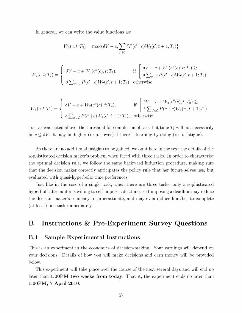
In general, we can write the value functions as:

W3(c, t;T3) = max{δV − c,∑c′∈C

δP (c′ | c)W3(c′, t+ 1, T3)}

W2(c, t;T2) =

δV − c+W3(c′′(c), t;T3), if

[δV − c+W3(c′′(c), t;T3) ≥δ∑

c′∈C P (c′ | c)W2(c′, t+ 1;T2)

δ∑

c′∈C P (c′ | c)W2(c′, t+ 1;T2) otherwise

W1(c, t;T1) =

δV − c+W2(c′′(c), t;T2), if

[δV − c+W2(c′′(c), t;T2) ≥δ∑

c′∈C P (c′ | c)W1(c′, t+ 1;T1)

δ∑

c′∈C P (c′ | c)W1(c′, t+ 1;T1), otherwise

Just as was noted above, the threshold for completion of task 1 at time T1 will not necessarily

be c ≤ δV . It may be higher (resp. lower) if there is learning by doing (resp. fatigue).

As there are no additional insights to be gained, we omit here in the text the details of the

sophisticated decision maker’s problem when faced with three tasks. In order to characterise

the optimal decision rule, we follow the same backward induction procedure, making sure

that the decision maker correctly anticipates the policy rule that her future selves use, but

evaluated with quasi-hyperbolic time preferences.

Just like in the case of a single task, when there are three tasks, only a sophisticated

hyperbolic discounter is willing to self-impose a deadline: self-imposing a deadline may reduce

the decision maker’s tendency to procrastinate, and may even induce him/her to complete

(at least) one task immediately.

B Instructions & Pre-Experiment Survey Questions

B.1 Sample Experimental Instructions

This is an experiment in the economics of decision-making. Your earnings will depend on

your decisions. Details of how you will make decisions and earn money will be provided

below.

This experiment will take place over the course of the next several days and will end no

later than 1:00PM two weeks from today. That it, the experiment ends no later than

1:00PM, 7 April 2010.

57

The Tasks

You will be given three tasks to be completed over the internet. While the tasks are not

specifically related to each other, they can only be completed sequentially (that is, you may

only work on one task at a time).

For each task, you will be given a list of 150 words which have been arranged randomly

and you will be asked to enter them on a computer terminal in alphabetical order. An

example is shown in Figure 13.

Figure 13: Experimental Interface For Tasks 18/03/2010 13:38http://cess.nyu.edu/web_experiments/ny/participant/task.php

Page 1 of 2

1

2

3

4

5

6

7

8

9

10

11

12

13

14

15

16

17

18

19

20

21

22

23

24

25

26

27

28

29

30

31

32

33

34

35

36

37

38

39

40

41

42

43

76

77

78

79

80

81

82

83

84

85

86

87

88

89

90

91

92

93

94

95

96

97

98

99

100

101

102

103

104

105

106

107

108

109

110

111

112

113

114

115

116

117

118

This is This is Task 1.Task 1.In order to complete this task you must solve the problem given to you by entering the words below inIn order to complete this task you must solve the problem given to you by entering the words below inalphabetical order, with the following restrictions:alphabetical order, with the following restrictions:

You must complete Task 1 by 10:00 pm on Monday, April 5, 2010.You must complete Task 1 by 10:00 pm on Monday, April 5, 2010.You must solve this problem by 04:25 pm, or you will be issued a new one.You must solve this problem by 04:25 pm, or you will be issued a new one.If you refresh your browser, or if you close your browser and log in again at a later time, you will beIf you refresh your browser, or if you close your browser and log in again at a later time, you will beissued a new problem.issued a new problem.

Select the Select the SubmitSubmit button at the bottom of this page to submit the solution to you problem. button at the bottom of this page to submit the solution to you problem.

For each task properly completed, by the appropriate time, you will be paid $15. Details

of how you will be paid will be given later.

58

The Interface

• This experiment will take place over the internet. Any time that you wish to work on

a task, simply go to the following website:

http://www.cess.nyu.edu/web_experiments/ny

• Upon arriving at the website, you will be prompted for your user ID and password.

Shortly, you will be provided with a user ID and password. Please keep the sheet of

paper on which your user ID and password are written as this is your only means of

gaining access to the experimental software.

• Once you have logged into the system, you may now work on a task.

• As can be seen in Figure 13, the list of words is given in the center of the screen and

words are entered alphabetically at the left and right. The earliest word alphabetically,

should be entered in the cell labeled 1.

• When you have completed a task (i.e., when you have arranged all words in the proper

order), press the submit button, which is at the bottom of the screen.

• If you have done it correctly, then you will be taken to a new screen where, if you

choose, you may work on the next (if any) task.

• If there are mistakes, you will be told:

The list you submitted contains one or more errors.

and remain on the screen for the current task. Observe that you will not be told the

nature of the mistakes, simply that the task has not been properly completed.

• Once you have been issued a list of words to alphabetize for a particular task, then

you must complete it within 2 hours (or before the deadline for that task, whichever

is earlier). If you do not complete the task within this time, you will be given a new

list of words.

• Note that if you press the refresh button or close the web browser and return later,

you will be given a new list of words.

59

http://www.cess.nyu.edu/web_experiments/ny

Completing the Tasks

Of course, there are many different ways that one might wish to approach this task. One

way that we have found to work reasonably well is to print the screen containing the words,

enter the words into a spreadsheet application such as Excel (Microsoft), Numbers (Apple)

or Calc (Open Office), use the sort command and then enter the words in the appropriate

order through the experimental interface. If you are careful with this method, then it should

be possible to complete each task in 1 hour or less.

deadlines

As indicated above, the experiment will end no later than 1:00PM, 7 April 2010. That

is, all tasks not correctly completed before this time will be considered incomplete and no

payments will be made incomplete tasks. However, if you wish, you may set a separate

deadline for each of the tasks. If you do so, the deadline must be no earlier than 1:00PM

today and no later than 1:00PM, 7 April 2010. Also, the deadline for Task 2 must be the

same or after the deadline for Task 1, and similarly for Task 3.

It is important to note that the deadlines will be strictly enforced. For example, if you

impose a deadline of 8:26PM tomorrow for the first task and do not complete it by that

time, you will not receive any payment for this task. However, if you miss a deadline for

one task, you will be permitted to move immediately to the subsequent task. That is, if you

miss the deadline for Task 1, you may proceed immediately to Task 2 provided that there is

still time remaining in the experiment and its deadline has also not passed.

At the appropriate time, once you have logged in to the experimental software, you will

enter your deadlines for each of the tasks. The interface for this is displayed in Figure 14.

Payment

For each task that you have properly completed by the appropriate deadline, you will be

paid $15. When you have completed a task, the experimental software will immediately

notify one of the experimenters that a task has been completed. For all tasks which have

been completed by 1:00PM on any given day, the experimenter will write a check and place

it in the mail by the end of the day. Payments for any tasks completed after the 1:00PM

cutoff will be processed and mailed the next day.

Questions

If there are any questions, please ask them now. If not, we will now provide a demonstration

of the experimental software and also provide you with your user ID and password.

60

Figure 14: Experimental Interface For Choosing deadlines

18/03/2010 13:34http://cess.nyu.edu/web_experiments/ny/participant/deadline.php

Page 1 of 1

DeadlinesDeadlines

Please read carefully

The experiment ends on April 07 (Wed), 2010 at 01:00 pm .However, you may impose an earlier deadline (for each task) if you wish. If so,please do so now. Keep in mind that the deadlines will be strictly enforced. For example, if you impose a deadline of Mar 19 (Fri), 2010 at02:00 am for the first task and do not complete the task by that time, you will not receive any payment for its completion.

Set Deadlines For Task 1

Enter Date: (MM/DD/YYYY)

Enter Time: PM (HH:MM (AM/PM))







Submit

B.2 Survey Questions

1. How many courses are you taking?

2. What is your major?

3. What is your GPA?

4. Over the course of the next two weeks, how many of each of the following to you have:

(a) minor assignments?

(b) major assignments or term papers?

(c) exams?

5. In response to the question above, please list the due dates for each assignment and

the date of any exams you have in the next two weeks.

6. Are you presently employed?

7. How many social, academic or sports clubs do you belong to?

8. Over the course of the next two weeks, how much time (in hours) do you expect to

allocate to:

61

(a) your course work?

(b) your job?

(c) social obligations or recreational activities?

(d) family obligations?

9. In response to Question 8(a), please provide details of your work schedule over the

next two weeks.

10. In response to Question 8(b), please provide the dates for which you plan to participate

in social or recreational activities.

11. In response to Question 8(c), please provide the dates for which you have planned

family obligations.

12. On a scale from 1 to 5 with 1 being “hardly at all” and 5 being “very much so”, please

answer the following questions:

(a) How conscientious are you?

(b) How often are you late turning in assignments?

(c) How often are you on time for appointments?

13. On a scale from 1 to 5 with 1 being “strongly disagree” and 5 being “strongly agree”,

rate how closely you identify with the following statements:

(a) Unexpected things which require my time and attention always seem to occur.

(b) Sometimes I am not as dependable or reliable as I should be.

(c) I follow a schedule.

(d) I never seem to be able to get organised.

(e) I always pay attention to details.

Suppose that you win 10 certificates, each of which can be used (once) to receive a

dream restaurant night. On each such night, you and a companion will get the best

table and an unlimited budget for food and drink at a restaurant of your choosing.

There will be no cost to you: all payments including gratuities come as part of the

prize. The certificates are available for immediate use, starting tonight, and there is

an absolute guarantee that they will be honored by any restaurant you select if they

are used within a two year window. However if they are not used up within this two

year period, any that remain are valueless.

62

The questions below concern how many of the certificates you would ideally like to

use in each year, how tempted you would be to depart from this ideal, and what you

expect you would do in practice:

14. From your current perspective, how many of the ten certificates would you ideally like

to use in year 1?

15. Continue with the scenario of Question 14. Some people might be tempted to depart

from their ideal allocation in Question 14. Which of the following best describes you:

(a) I would have no temptation in either direction.

(b) I would be somewhat/strongly tempted to use more certificates in the first year

than would be ideal.

(c) I would be strongly/somewhat tempted to keep more certificates for use in the

second year than would be ideal.

16. Continue with the scenario of Question 14. If you were to give in to your temptation,

how many certificates do you think you would use in year 1 as opposed to year 2?

17. Continue with the scenario of Question 14. Based on your most accurate forecast of

how you think you would actually behave, how many of the nights would you end up

using in year 1?

18. On a scale from 0 to 100, how likely do you think each of the following events are?

(a) I will complete no tasks.

(b) I will complete at least one task.

(c) I will complete at least two tasks.

(d) I will complete all three tasks.

63

Present-Bias, Procrastination and Deadlines in a Field ... · Present-Bias, Procrastination and...

Documents

Transcript of Present-Bias, Procrastination and Deadlines in a Field ... · Present-Bias, Procrastination and...