Preprocessing of FMRI Data fMRI Graduate Course October 23, 2002.
42
Preprocessing of FMRI Data fMRI Graduate Course October 23, 2002
-
Upload
emerald-goodwin -
Category
Documents
-
view
226 -
download
0
Transcript of Preprocessing of FMRI Data fMRI Graduate Course October 23, 2002.

Preprocessing of FMRI Data
fMRI Graduate Course
October 23, 2002

What is preprocessing?
• Correcting for non-task-related variability in experimental data– Usually done without consideration of
experimental design; thus, pre-analysis– Occasionally called post-processing, in
reference to being after acquisition
• Attempts to remove, rather than model, data variability
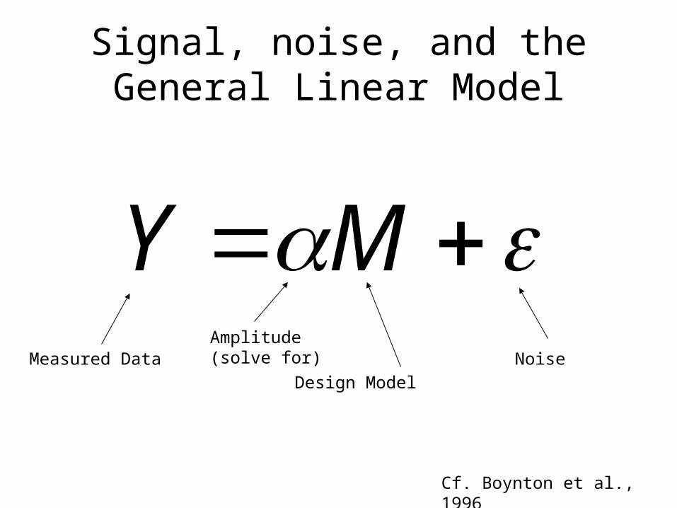
Signal, noise, and the General Linear Model
MYMeasured Data
Amplitude (solve for)
Design Model
Noise
Cf. Boynton et al., 1996

Signal-Noise-Ratio (SNR)
Task-Related Variability
Non-task-related Variability
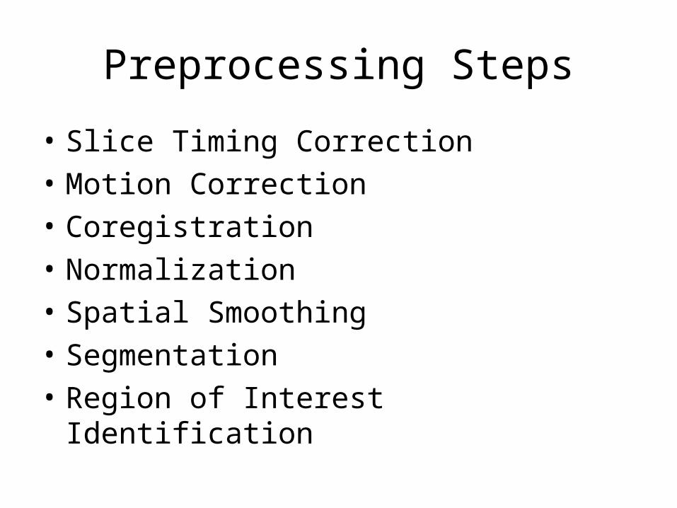
Preprocessing Steps
• Slice Timing Correction
• Motion Correction
• Coregistration
• Normalization
• Spatial Smoothing
• Segmentation
• Region of Interest Identification
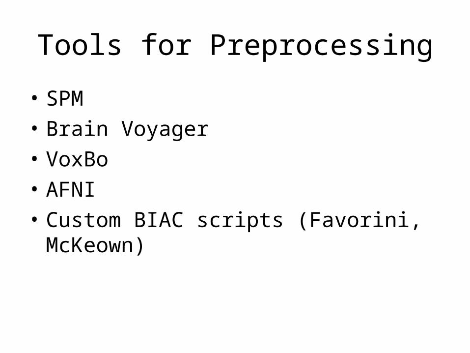
Tools for Preprocessing
• SPM
• Brain Voyager
• VoxBo
• AFNI
• Custom BIAC scripts (Favorini, McKeown)

Slice Timing Correction

Why do we correct for slice timing?
• Corrects for differences in acquisition time within a TR– Especially important for long TRs (where expected HDR
amplitude may vary significantly)– Accuracy of interpolation also decreases with increasing TR
• When should it be done?– Before motion correction: interpolates data from (potentially)
different voxels• Better for interleaved acquisition
– After motion correction: changes in slice of voxels results in changes in time within TR
• Better for sequential acquisition
Effects of uncorrected slice timing
• Base Hemodynamic Response
• Base HDR + Noise
• Base HDR + Slice Timing Errors
• Base HDR + Noise + Slice Timing Errors

Base HDR: 2s TR
0
0.2
0.4
0.6
0.8
1
1.2
TR:-1 TR:0 TR:1 TR:2 TR:3 TR:4 TR:5
Slice1
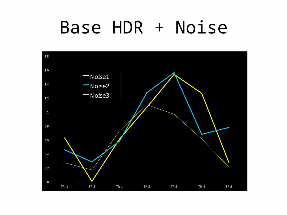
Base HDR + Noise
0
0.2
0.4
0.6
0.8
1
1.2
1.4
1.6
1.8
TR:-1 TR:0 TR:1 TR:2 TR:3 TR:4 TR:5
Noise1
Noise2
Noise3
r = 0.77
r = 0.80
r = 0.81

0
0.2
0.4
0.6
0.8
1
1.2
TR:-1 TR:0 TR:1 TR:2 TR:3 TR:4 TR:5
Slice1
Slice11
Slice12
Base HDR + Slice Timing Errors
r = 0.85r = 0.92
r = 0.62

HDR + Noise + Slice Timing
0
0.2
0.4
0.6
0.8
1
1.2
1.4
1.6
1.8
TR:-1 TR:0 TR:1 TR:2 TR:3 TR:4 TR:5
Slice1
Slice11
Slice12
r = 0.65
r = 0.67
r = 0.19

Interpolation Strategies
• Linear interpolation
• Spline interpolation
• Sinc interpolation

Motion Correction
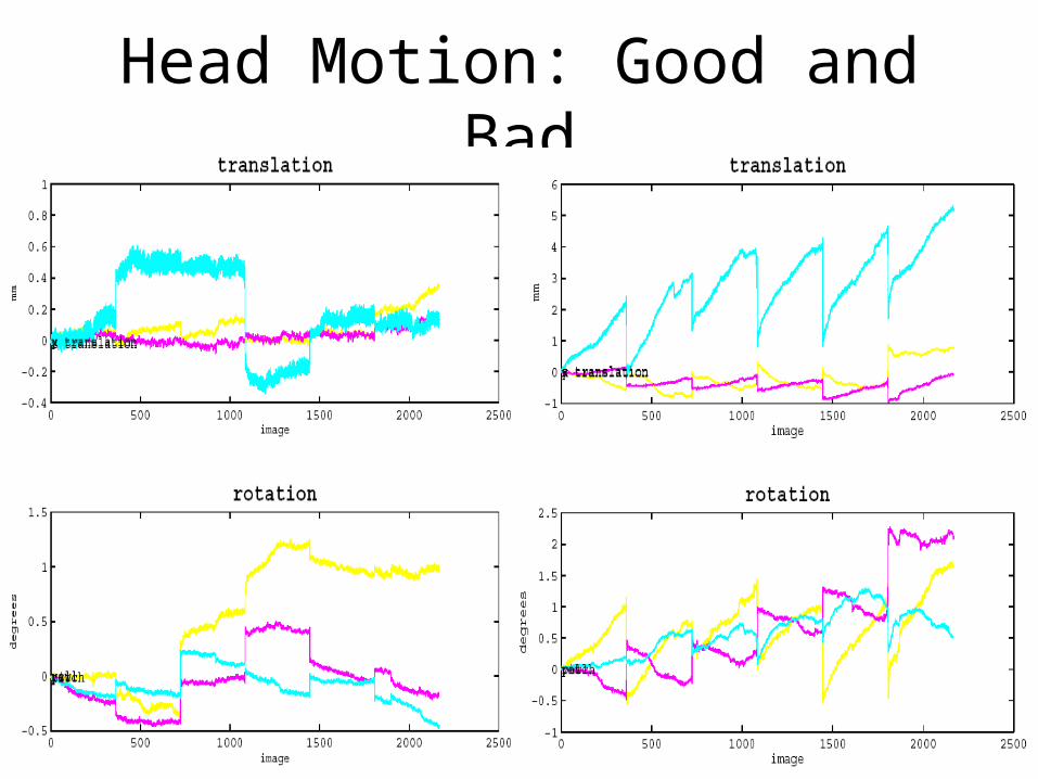
Head Motion: Good and Bad

Correcting Head Motion
• Rigid body transformation– 6 parameters: 3 translation, 3 rotation
• Minimization of some cost function– E.g., sum of squared differences

Simulated Head Motion

Severe Head Motion: Simulation
Two 4s movements of 8mm in -Y direction (during task epochs)
Motion
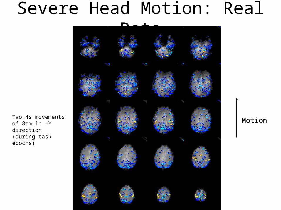
Severe Head Motion: Real Data
Two 4s movements of 8mm in –Y direction (during task epochs)
Motion

Effects of Head Motion Correction
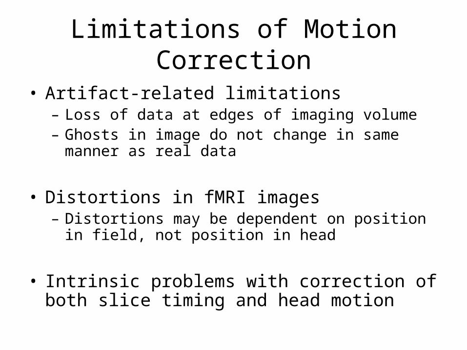
Limitations of Motion Correction
• Artifact-related limitations– Loss of data at edges of imaging volume– Ghosts in image do not change in same manner as
real data
• Distortions in fMRI images– Distortions may be dependent on position in field, not
position in head
• Intrinsic problems with correction of both slice timing and head motion
Coregistration

Should you Coregister?
• Advantages– Aids in normalization– Allows display of activation on anatomical images– Allows comparison across modalities– Necessary if no coplanar anatomical images
• Disadvantages– May severely distort functional data– May reduce correspondence between functional and
anatomical images

Normalization

Standardized Spaces
• Talairach space (proportional grid system)– From atlas of Talairach and Tournoux (1988)– Based on single subject (60y, Female, Cadaver)– Single hemisphere– Related to Brodmann coordinates
• Montreal Neurological Institute (MNI) space– Combination of many MRI scans on normal controls
• All right-handed subjects– Approximated to Talaraich space
• Slightly larger• Taller from AC to top by 5mm; deeper from AC to bottom by 10mm
– Used by SPM, National fMRI Database, International Consortium for Brain Mapping

Normalization to Template
Normalization Template Normalized Data

Anterior and Posterior Commissures
Anterior Commissure
Posterior Commissure

Should you normalize?
• Advantages– Allows generalization of results to larger population– Improves comparison with other studies– Provides coordinate space for reporting results– Enables averaging across subjects
• Disadvantages– Reduces spatial resolution– May reduce activation strength by subject averaging– Time consuming, potentially problematic
• Doing bad normalization is much worse than not normalizing

Slice-Based Normalization
Before Adjustment (15 Subjects)
After Adjustment to Reference Image
Registration courtesy Dr. Martin McKeown (BIAC)

Spatial Smoothing

Techniques for Smoothing
• Application of Gaussian kernel– Usually expressed in
#mm FWHM– “Full Width – Half
Maximum”– Typically ~2 times
voxel size

Effects of Smoothing on Activity
Unsmoothed Data
Smoothed Data (kernel width 5 voxels)
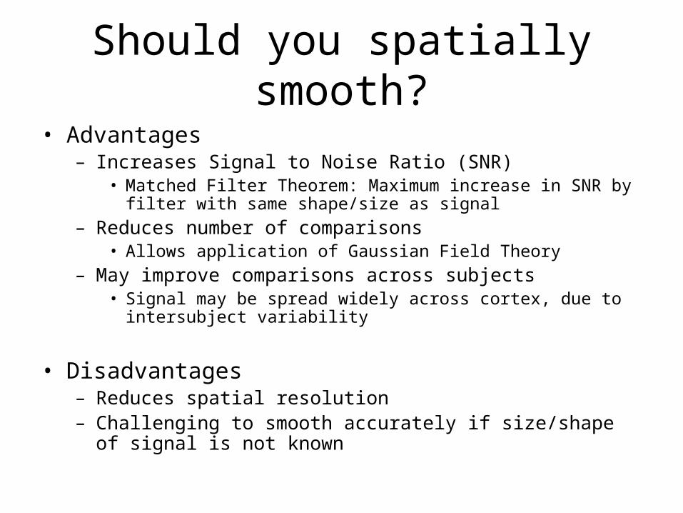
Should you spatially smooth?
• Advantages– Increases Signal to Noise Ratio (SNR)
• Matched Filter Theorem: Maximum increase in SNR by filter with same shape/size as signal
– Reduces number of comparisons• Allows application of Gaussian Field Theory
– May improve comparisons across subjects• Signal may be spread widely across cortex, due to intersubject
variability
• Disadvantages– Reduces spatial resolution – Challenging to smooth accurately if size/shape of signal is not
known
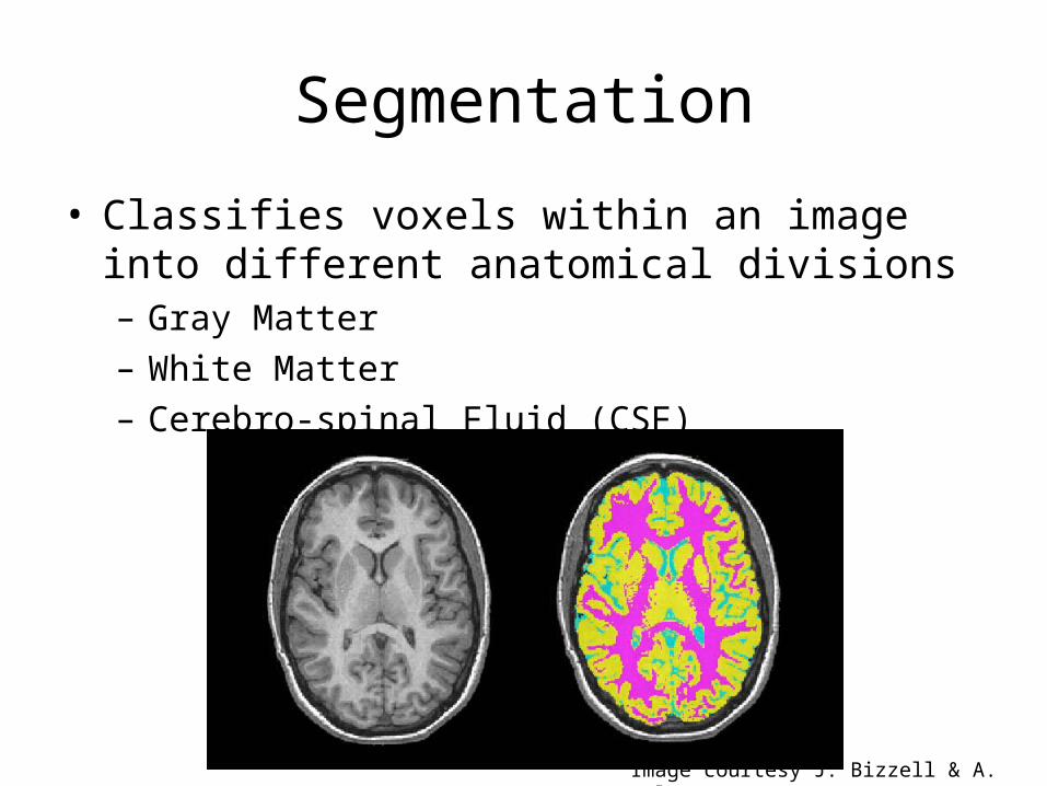
Segmentation
• Classifies voxels within an image into different anatomical divisions– Gray Matter– White Matter– Cerebro-spinal Fluid (CSF)
Image courtesy J. Bizzell & A. Belger

Histogram of Voxel Intensities
0
0.005
0.01
0.015
0.02
0.025
0.03
0.035
0.04
Anatomical
Functional

Region of Interest Drawing

Why use an ROI-based approach?
• Allows direct, unbiased measurement of activity in an anatomical region– Assumes functional divisions tend to follow
anatomical divisions
• Improves ability to identify topographic changes– Motor mapping (central sulcus)– Social perception mapping (superior temporal sulcus)
• Complements voxel-based analyses
Drawing ROIs
• Drawing Tools– BIAC software (e.g., Overlay2)– Analyze– IRIS/SNAP (G. Gerig)
• Reference Works– Print atlases– Online atlases
• Analysis Tools– roi_analysis_script.m

ROI Examples

-2
-1
0
1
2
3
4
-3-1
.5 01
.5 34
.5 67
.5 91
0.5 12
13
.5 15
16
.5 -3-1
.5 01
.5 34
.5 67
.5 91
0.5 12
13
.5 15
16
.5 -3-1
.5 01
.5 34
.5 67
.5 91
0.5 12
13
.5 15
16
.5 -3-1
.5 01
.5 34
.5 67
.5 91
0.5 12
13
.5 15
16
.5 -3-1
.5 01
.5 34
.5 67
.5 91
0.5 12
13
.5 15
16
.5 -3-1
.5 01
.5 34
.5 67
.5 91
0.5 12
13
.5 15
16
.5 -3-1
.5 01
.5 34
.5 67
.5 91
0.5 12
13
.5 15
16
.5 -3-1
.5 01
.5 34
.5 67
.5 91
0.5 12
13
.5 15
16
.5 -3-1
.5 01
.5 34
.5 67
.5 91
0.5 12
13
.5 15
16
.5 -3-1
.5 01
.5 34
.5 67
.5 91
0.5 12
13
.5 15
16
.5 -3-1
.5 01
.5 34
.5 67
.5 91
0.5 12
13
.5 15
16
.5 -3-1
.5 01
.5 34
.5 67
.5 91
0.5 12
13
.5 15
16
.5 -3-1
.5 01
.5 34
.5 67
.5 91
0.5 12
13
.5 15
16
.5
80 75 70 65 60 55 50 45 40 35 30 25 20
Distance Posterior from the Anterior Commissure (in mm)
Left Hemisphere - Gaze Shifts Right Hemisphere - Gaze Shifts
60 55 50 45 40 35 30 25 20 15 10 5 0
BIAC is studying biological motion and social perception – here by determining how context modulates brain activity in elicited when a subject watches a character shift gaze toward or away from a target.
Additional Resources
• SPM website– Course Notes
• http://www.fil.ion.ucl.ac.uk/spm/course/notes01.html
– Instructions
• Brain viewers– http://www.bic.mni.mcgill.ca/cgi/icbm_view/