1

PREPRINT DEPARTMENT OF PHYSICS AND

ELECTRONICS,UNIVERSITY OF PUERTO RICO AT HUMACAO

EARTH AND MARS CRATER-SIZE FREQUENCY DISTRIBUTION AND

IMPACT RATES:THEORETICAL AND OBSERVATIONAL ANALYSIS

W. BRUCKMAN, A. RUIZ, E. RAMOS William Bruckman , Abraham Ruiz : Department of Physics and Electronics , And

Elio Ramos : Department of Mathematics , University of Puerto Rico At Humacao

2

ABSTRACT

A framework for the theoretical and analytical understanding of the impact crater-size frequency distribution is developed and applied to observed data from Mars and Earth. The analytical model derived gives the crater population as a function of crater diameter, 𝐷 , and age, 𝜏, taking into consideration the reduction in crater number as a function of time, caused by the elimination of craters due to effects such as erosion, obliteration by other impacts, and tectonic changes. When applied to Mars, using Barlow’s impact crater catalog, we are able to determine an analytical curve describing the number of craters per bin size, 𝑁(𝐷), which perfectly reproduces and explains the presence of two well-defined slopes in the log[𝑁] 𝑣𝑠 log [𝐷] plot. For craters with 𝐷 ≤ ~57𝑘𝑚, we find that 𝑁 𝛼 1/𝐷1.8, and this distribution corresponds to ’saturation’, where the rate of production is equal to the rate of destruction of craters. A steeper slope, with 𝑁𝛼 1/𝐷4.3 is found for the larger craters, 𝐷 ≥ ~57𝑘𝑚 , from which it is interpreted that 𝑁 is pristine, or essentially unaffected by destructive mechanisms. Since in this limit of larger 𝐷 the rate of impacts, 𝛷(𝐷), is proportional to 1

𝐷4.3, and the cumulative rate, 𝛷𝐶(𝐷) ≡ ∫ 𝛷𝑑𝐷∞𝐷 , is proportional to 1/𝐷3.3, we are able to estimate that

the rate of meteorite impacts for energies, 𝐸, of a megaton or above (𝐷 ≥ ~1𝑘𝑚 ) is about one every three years, a result that is relevant for future Mars explorations. The corresponding calculations for our planet give a probability of one per 15 years for an impact 𝐸 ≥ ~megaton, while for a Tunguska–like event, where 𝐸 = 10 megatons, an estimate of one per nearly a century is obtained. Our cumulative flux 𝛷𝐶 is also expressed as a function of the meteorite diameter,𝑑, and 𝐸, thus obtaining for Earth: 𝛷𝐶 = 5.5[1∓0.5]

106𝑦𝑒𝑎𝑟𝑠 𝑑2.57 = [1∓0.5]14.5𝑦𝑒𝑎𝑟𝑠 𝐸0.86, where 𝑑 is in kilometers, and 𝐸 in megatons,

results that are similar to those of Poveda et al (1999). The model allows the derivation of a more general expression, 𝑁�, that gives the number of craters observed today in the grid of diameters between 𝐷 and 𝐷 + ∆𝐷 and with an age between 𝜏 and 𝜏 + ∆𝜏. The applicationof 𝑁� to describe the Earth’s crater data shows a remarkable agreement between theory and observations.

3

1. Introduction and Summary

The present impact crater-size frequency distribution, 𝑁(𝐷), is the result, on one hand, of the rate of crater formation 𝛷 attributed to the impacts of asteroids and comets, and, on the other hand, of the elimination of craters as they get older, by processes like erosion, obliteration by other impacts, tectonic changes, etc. Therefore, in order to understand the history of crater formation we will, in section 2, combine the above creation and elimination factors to show that we can express 𝑁(𝐷) in terms of 𝛷 and the mean-life of a crater of diameter 𝐷, 𝜏𝑚𝑒𝑎𝑛. Then, a simple model based on the above considerations is discussed in section 3, where we describe the crater-size distribution for planet Mars data, collected by Barlow (Barlow, 1988), and find that 𝛷� 𝛼 𝐷−4.3 and 𝜏𝑚𝑒𝑎𝑛 𝛼 𝐷2.5 ,where 𝛷� is the time average of 𝛷.

In section 4 we use the above formalism to describe Earth’s crater data as a function of crater age 𝜏, and conclude that on our planet it is also true that 𝜏𝑚𝑒𝑎𝑛 𝛼 𝐷2.5. This interesting result is interpreted to mean that on the surface of both Mars and Earth, 𝜏𝑚𝑒𝑎𝑛 is approximately proportional to the volume of the crater ≡ 𝐷2ℎ, where ℎ is defined as the average height of the crater and accordingly satisfies ℎ 𝛼 𝐷1/2. Investigations of the geometric properties of a Martian impact crater (Garvin 2002) indeed confirm that ℎ(𝐷) ≅ 𝐷0.5.

Next, in section 5, we take on the calculation of 𝛷(𝐷) and 𝛷𝐶(𝐷) for our planet, where 𝛷𝐶(𝐷), ‘the cumulative flux’, is the rate of impact of craters with diameters larger than 𝐷. 𝛷𝐶 is also expressed as a function of the impactor diameter 𝑑 and its kinetic energy 𝐸 . For instance, our results predict one megaton or larger energy bolide with probable period of about one every 15/[1∓0.5] years, while nearly one Tunguska-like event (𝐸 ≥ 10 megatons) is expected every century: 105/[1∓0.5] years. Another interesting result is that, according to our model, a meteorite impact of catastrophic potential, 𝐷 ≥ ~5𝑘𝑚, 𝑑 ≥ ~0.2𝑘𝑚, is likely to have occurred within historical times: 𝜏 ≤ ~5,000 years. Generally speaking, we find that for our planet we have:

𝛷𝐶 = 2.8[1∓0.50𝑚𝑦

](20𝐷� )3.3 = 5.5[1∓0.5]

𝑚𝑦 𝑑2.57 = [1∓0.5]14.5𝑦 𝐸0.86,

where 𝑑 and 𝐷 are in kilometers, 𝐸 in megatons, and 𝑚𝑦 ≡ 106 years≡ 106𝑦. The above result is in almost perfect agreement with the results of Poveda et al (1999). We compare, in section 6, the fluxes of Earth and Mars, and conclude that astronauts on Mars will probably be subjected to a meteorite with at least a megaton of energy in a mission lasting more than about three years. This intriguing result raises concerns for manned missions to the red planet in the near future.

In the last section we consider an application of a general expression 𝑁�(𝐷,𝐷 + ∆𝐷, 𝜏, 𝜏 + ∆𝜏) to Earth, that gives the number of craters observed today in the grid of diameters between 𝐷 and 𝐷 + ∆𝐷 and with an age between 𝜏 and 𝜏 + ∆𝜏. First, in Table III and Figure (5), 𝑁�(𝜏) is calculated for craters older than 𝜏, 1𝑚𝑦 ≤ 𝜏 ≤ 2,500𝑚𝑦, and for all diameters≥ 20𝑘𝑚, and this is compared with the observations. The crater data was obtained from http://www.passc.net/EarthImpactDatabase/, where we used 𝐷 ≥ 20𝑘𝑚 and the following selected area to minimize the undercounting of craters: Australia, Europe, Canada up to the Arctic Circle latitude and the United States. We found that the theoretical 𝑁�(𝜏) remarkably reproduces the observed data. Furthermore, in Table IV and Figure (6) we again compare the theory and observations, this time for craters of all ages but with

4

𝑁�(𝑑𝑖𝑎𝑚𝑒𝑡𝑒𝑟𝑠 ≥ 𝐷) vs. 𝐷, ( 1𝑘𝑚 ≤ 𝐷 ≤ 300𝑘𝑚 ). Here we see, as expected, a discrepancy with observational data for 𝐷 ≤ ~20𝑘𝑚, due to undercounting, but a very good agreement for 𝐷 ≥ 20𝑘𝑚.

2. Theoretical Model for the Observed Data

In what follows, we will present a theoretical and analytical curve that will reproduce the essential features of the Martian crater-size frequency distribution empirical curve (Figure (1)), based on Barlow’s (1988) database of about 42,000 impact craters. The models will be derived using reasonably simple assumptions, which will allow us to relate the present crater population to the crater population at each particular epoch.

To this end, let ∆𝑁(𝐷, 𝑡)∆𝐷 represent the number of craters of diameter 𝐷 ∓ ∆𝐷/2 formed during the epoch 𝑡 ∓ ∆𝑡/2, where we are assuming that ∆𝑡 and ∆𝐷 are sufficiently large to justify treating ∆𝑁 as a statistically continuous function, but sufficiently small to be able to treat them as differential in the following discussion. This initial population will change as time goes on due to climatic and geological erosion and the obliteration of old craters by the formation of new ones. Therefore, we expect that the change in ∆𝑁 during a time interval dt will be proportional to itself and dt:

𝑑(∆𝑁) = −𝐶∆𝑁𝑑𝑡 (1)

where 𝐶 is a factor that takes into account the depletion of the craters, and should be a function of the diameter, since the smaller a crater is, the more likely it is to disappear. It is easy to integrate Eq. (1) in time to obtain

∆𝑁(𝐷, 𝑡) = ∆𝑁(𝐷, 𝑡𝑛)𝐸𝑥𝑝[−𝐶̅𝜏𝑛], (2)

𝐶̅𝜏𝑛=∫ 𝐶𝑡𝑡𝑛

𝑑𝑡`, (3)

𝜏𝑛 ≡ 𝑡 − 𝑡𝑛, (4)

which is the familiar equation for an exponential decay of ∆𝑁 with mean-life: 𝜏𝑚𝑒𝑎𝑛 = 1/𝐶̅.

Eq. (2) gives the number of craters, per bin size, as a function of diameter, that are observed at time 𝑡 but were produced in the time interval 𝑡𝑛 ∓ ∆𝜏𝑛/2. Therefore, the total contribution to the present (𝑡 = 0) population of craters is:

𝑁(𝐷, 0) ≡ 𝑁(𝐷) = ∑ ∆𝑁(𝐷, 𝑡𝑛𝑛 )𝐸𝑥𝑝[−𝐶̅𝜏𝑛] = ∑ [∆𝑁(𝐷, 𝑡𝑛𝑛 )/∆𝜏𝑛]𝐸𝑥𝑝[−𝐶̅𝜏𝑛]∆𝜏𝑛. (5)

Alternatively, in the continuous limit ∆𝜏𝑛 → 𝑑𝜏 → 0, Eq. (5) becomes

𝑁(𝐷) = ∫ {𝛷(𝐷, 𝜏)𝜏𝑓0 𝐸𝑥𝑝[−𝐶̅𝜏]}𝑑𝜏, (6)

where

𝛷(𝐷, 𝜏) ≡ lim∆𝜏𝑛→0(∆𝑁(𝐷, 𝜏𝑛)/∆𝜏𝑛). (7)

5

We see that 𝛷(𝐷, 𝜏) corresponds to the rate of formation of craters per bin size, of diameter 𝐷 in the epoch 𝜏, and 𝜏𝑓 is the total time of crater formation.

Another derivation of Eq. (6) is as follows. The number of craters formed over time 𝑑𝑡 is 𝛷𝑑𝑡, while the craters eliminated in this time are 𝐶𝑁𝑑𝑡. Therefore, the net change in 𝑁 is

𝑑𝑁 = 𝛷𝑑𝑡 − 𝐶𝑁𝑑𝑡, (8)

which is an equation that can be integrated by an elementary method, illustrated below. Multiplying the above equation by 𝐸𝑥𝑝[−∫ 𝐶𝜏0 𝑑𝜏`] ≡ 𝐸𝑥𝑝[−𝐶̅𝜏], with 𝜏 = −𝑡, we arrive at

𝐸𝑥𝑝[−𝐶̅𝜏](𝑑𝑁 − 𝐶𝑁𝑑𝜏) = −𝐸𝑥𝑝[−𝐶̅𝜏](𝛷𝑑𝜏), (9)

which, after using

𝑑(𝐶̅𝜏) ≡ 𝑑 ∫ 𝐶𝜏0 𝑑𝜏` = 𝐶𝑑𝜏, (10)

becomes

𝑑(𝑁𝐸𝑥𝑝[−𝐶̅𝜏]) = −𝐸𝑥𝑝[−𝐶̅𝜏](𝛷𝑑𝜏). (11)

Integrating Eq. (11) from 0 to 𝜏𝑓 with 𝑁(𝜏𝑓) = 0 gives Eq. (6). Note that if, instead of the time interval 𝜏 = 0 to 𝜏 = 𝜏𝑓 in Eq. (6), we have the arbitrary limits 𝜏 to 𝜏 + ∆𝜏, we obtain the more general expression:

𝑁(𝐷, 𝜏, 𝜏 + ∆𝜏) = ∫ {𝛷(𝐷, 𝜏`)𝜏+∆𝜏𝜏 𝐸𝑥𝑝[−𝐶̅𝜏`]}𝑑𝜏`. (12)

The 𝑁 defined in Eq. (6) represents the number of craters of diameter 𝐷 per bin size observed today (𝑡 = 0) that are younger than age 𝜏𝑓, while in Eq. (12) 𝑁 represents the number of craters observed at 𝑡 = 0 formed, per bin, in the time interval 𝜏 to 𝜏 + ∆𝜏. Accordingly, the number of present craters in an arbitrary diameter interval 𝐷 to 𝐷 + ∆𝐷 with age between 𝜏 and 𝜏 + ∆𝜏 is represented by the integral:

𝑁�(𝐷,𝐷 + ∆𝐷, 𝜏, 𝜏 + ∆𝜏) ≡ ∫ 𝑁(𝐷, 𝜏, 𝜏 + ∆𝜏)𝑑𝐷𝐷+∆𝐷𝐷 . (13)

For instance, if ∆𝐷 → ∞ , the integral is called the total cumulative number of craters. Further discussions and applications of Eq. (13) to the Earth’s crater record will be continued in section 7. For planet Mars, however, we will be applying Eq. (6) in the next section.

6

3. Applications to Mars

In Appendix A we show that Eq. (6) can be rewritten in the form:

𝑁 = (𝛷/𝐶������){1 − 𝐸𝑥𝑝�−𝐶̅𝜏𝑓�}, (14)

where

𝛷/𝐶������) ≡ ∫ (𝛷(𝜏`)/𝐶){𝐸𝑥𝑝[−∫ 𝐶(𝜏``)𝑑𝜏``]}𝐶𝑑𝜏`𝜏`0

𝜏0

∫ {𝐸𝑥𝑝[−∫ 𝐶(𝜏``)𝑑𝜏``]}𝐶𝑑𝜏`𝜏`0

𝜏0

. (15)

Notice that (𝛷/𝐶������) is the weighted average of ( 𝛷 𝐶� ), with weight:

∫ {𝐸𝑥𝑝[−∫ 𝐶(𝜏``)𝑑𝜏``]}𝐶𝑑𝜏`𝜏`0

𝜏0 . (16)

We now consider Barlow’s (1988) data for Mars' crater-diameter distribution, which is plotted in Figure (1). Then the simplest model that describes these data, for 𝐷 ≥ 8𝑘𝑚, is given by the expressions (Figure (2)):

(𝛷/𝐶������) =1.43𝑥105

𝐷1.8 , (17)

𝐶̅ = ( 1𝜏𝑓

) 2.48𝑥104

𝐷2.5 , (18)

𝛷� = ( 1𝜏𝑓

) 3.55𝑥109

𝐷4.3 . (19)

(𝛷/𝐶������) = 𝛷�

𝐶̅ (20)

FIGURE (1): Log-Log plot of number of craters per bin, 𝑁(𝐷) 𝑣𝑠 𝐷 based on Barlow’s Mars catalog. The number 𝑁(𝐷) is calculated by counting the number of craters in a bin ∆𝐷 = 𝐷𝑅 − 𝐷𝐿, and then dividing this number by the bin size. The point is placed at the mathematical average of 𝐷 in the bin: (𝐷𝑅 + 𝐷𝐿)/2. The

bin size is ∆𝐷 = (√2− 1)𝐷𝐿, so that 𝐷𝑅𝐷𝐿

= √2.

7

FIGURE (2): Comparing the model in Eqs. (14) to (20) with the Mars data in Figure (1).

We see that the theoretical curve shown in Figure (2) differs significantly from the observed data for 𝐷 less than about 8𝑘𝑚. However, according to Barlow, her empirical data undercounts the actual crater population for 𝐷 less than 8𝑘𝑚 and therefore, we will restrict our analysis to 𝐷 ≥ 8𝑘𝑚.

Eqs. (2) and (18) imply that the fraction of craters of diameter 𝐷 formed at each epoch 𝜏 that still survive at the present time 𝑡 = 0 is given by:

∆𝑁(𝐷,0)∆𝑁(𝐷,𝜏)

= 𝐸𝑥𝑝[−𝐶̅𝜏] ≈ 𝐸𝑥𝑝[−(57/𝐷)2.5 𝜏𝜏𝑓

] (21)

and thus, the mean life for craters of diameter 𝐷, 𝜏𝑚𝑒𝑎𝑛 ≡ 𝐶̅−1, is:

𝜏𝑚𝑒𝑎𝑛 ≡ 𝐶̅−1 ≈ (𝐷/57)2.5 𝜏𝑓. (22)

Hence, craters with 𝐷 ≈ 57𝑘𝑚 have 𝜏𝑚𝑒𝑎𝑛 ≈ 𝜏𝑓, whereas

𝜏𝑚𝑒𝑎𝑛 ≫ 𝜏𝑓 , 𝐷 ≫ 57𝑘𝑚, (23)

𝜏𝑚𝑒𝑎𝑛 ≪ 𝜏𝑓 , 𝐷 ≪ 57𝑘𝑚. (24)

In the limit 𝐷 ≫ 57𝑘𝑚,𝐶̅𝜏𝑓 ≪ 1, we obtain, from Eqs. (14),(20) and (19), that:

𝑁 = 𝛷�𝜏𝑓 = 3.55𝑥109

𝐷4.3 ; 𝐶̅𝜏𝑓 ≪ 1, 𝐷 ≫ 57𝑘𝑚, (25)

which corresponds to a straight line of slope -4.3 in the log(𝑁) vs. log (𝐷) plot, which we see in the right-hand part of Figure (2), and is the form of Eq. (14) when we can ignore the destruction of craters (𝐶𝜏𝑓 ≪ 1). In other words, for these larger craters, their number is simply given by:

𝑁 = 𝛷�𝜏𝑓 ≡ ∫ 𝛷𝑑𝜏𝜏𝑓0 , (26)

an expected relationship when craters are conserved and therefore, when the actual crater number is proportional to the age of the underlying surface 𝜏𝑓. On the other hand, for smaller craters where 𝐸𝑥𝑝[−𝐶̅𝜏𝑓] ≪ 1 we will have, from Eqs. (14) and (17),

8

𝑁 = (𝛷/𝐶������) = 𝛷�

𝐶̅≡ 𝛷�𝜏𝑚𝑒𝑎𝑛 = 1.43𝑥105

𝐷1.8 , (27)

and hence in this limit, 𝑁 is proportional to the survival mean life, 𝜏𝑚𝑒𝑎𝑛, of craters of size 𝐷. This feature was called the ‘crater retention age’ by Hartmann (2002) and on Mars is shown in craters with 𝐷 less than about 57𝑘𝑚, corresponding to the straight line segment on the left-hand side of Figure (2) with slope -1.8. When this condition arises, 𝑁(𝐷) is independent of 𝜏, since crater production, 𝛷d𝑡, is balanced by crater destruction, 𝑁𝐶𝑑𝜏, and thus, from Eq. (8) we have:

𝑑𝑁 = 𝛷𝑑𝑡 − 𝐶𝑁𝑑𝑡 = 0, (28)

or, equivalently,

𝑁 = 𝛷𝐶. (29)

We see that the time average of Eq. (29) gives rise to Eq. (27). Therefore, the above model tells us that the empirical curve is essentially constructed by the following two straight lines in the 𝑙𝑜𝑔𝑁(𝐷) 𝑣𝑠 𝑙𝑜𝑔𝐷 plot:

𝑁(𝐷) = 𝛷�

𝐶̅= 1.43𝑥105

𝐷1.8 ; 𝐶̅𝜏𝑓 ≥ 1,𝐷 ≤ ~57𝑘𝑚, (30)

𝑁(𝐷) = 𝛷�𝜏𝑓 = 3.55𝑥109

𝐷4.3 ; 𝐶̅𝜏𝑓 ≤ 1,𝐷 ≥ ~57𝑘𝑚 . (31)

The exponent 4.3 is pristine, while the exponent 1.8 is the result of a steady state equilibrium between elimination and creation of craters. The large exponent, 4.3, has interesting implications for the corresponding impactors size-frequency distribution, and we will elaborate on this topic in section 5.

4. Determination of the Mean Life, 𝝉𝒎𝒆𝒂𝒏, of Impact Craters on Earth

In what follows, we will determine the mean life for craters on our planet. Let us first consider the expression defining the average diameter, with ages in a given bin time interval ∆𝜏 = 𝜏𝑅 − 𝜏𝐿, which is given by:

𝐷� = ∫ 𝐷𝑁(𝐷,𝜏𝐿,𝜏𝑅)𝑑𝐷∞0

∫ 𝑁(𝐷,𝜏𝐿,𝜏𝑅)𝑑𝐷∞0

, (32)

where, according to Eq. (12),

𝑁(𝐷, 𝜏𝐿 , 𝜏𝑅) ≡ ∫ 𝛷(𝐷, 𝜏){𝐸𝑥𝑝[−𝐶̅𝜏]}𝑑𝜏𝜏𝑅𝜏𝐿

. (33)

Investigations of the time dependence of the cratering rate of meteorites have concluded (see, for example, Hartmann (1966); Neukum et al (1983); Neukum (2001); Ryder (1990)) that the Earth went through a heavy bombardment era and that the impact rate then decayed exponentially until about 3,000 to 3,500 million years ago and since that time has remained nearly constant until the present. Therefore, for the Earth’s data which is younger than 3 to 3.5gy, we can reasonably assume that 𝛷

9

is independent of 𝜏. Furthermore, following the analysis of Mars, we also assume that 𝛷 and 𝐶̅ are given by the simple polynomial forms

𝛷 = 𝐴𝐷𝑚

;𝐴, 𝑚 𝑎𝑟𝑒 𝑐𝑜𝑛𝑠𝑡𝑎𝑛𝑡𝑠 , (34)

𝐶̅ = 𝐵𝐷𝑝

;𝐵 𝑎𝑛𝑑 𝑝 𝑎𝑟𝑒 𝑐𝑜𝑛𝑠𝑡𝑎𝑛𝑡𝑠. (35)

Then we can show (see Appendix C) that with 𝑔 ≡ 𝜏𝐿 𝜏𝑅� and 𝑚` ≡ 𝑚 − 𝑝, Eq. (32) becomes

𝐷� = (𝐵𝜏𝐿)1𝑝𝛼1, (36)

where:

𝛼1 = 𝛤((𝑚`−2) 𝑝)⁄𝛤((𝑚`−1) 𝑝)⁄

[1−𝑔(𝑚`−2) 𝑝⁄ ][1−𝑔(𝑚`−1) 𝑝⁄ ]

, (37)

and:

𝛤(𝑛) ≡ ∫ 𝑥𝑛−1∞0 𝑒−𝑥𝑑𝑥 (38)

is the complete Gamma function. Eq. (36) can be rewritten as

log[𝐷�] = �1𝑝� log [𝜏𝐿] + log [𝛼1𝐵

1𝑝], (39)

which is the equation for a straight line in the log[𝐷�] 𝑣𝑠 log[𝜏𝐿] graph, with a slope of 1/𝑝 and an

intercept log [𝛼1𝐵1𝑝] . In Figures (3) and (4) we plot log[𝐷�]𝑣𝑠 log [𝜏𝐿] , for 𝑔 = 1

2 and 𝑔 = 1/10

respectively, using the Earth’s crater size data against 𝜏. From Figure (3) we obtain 1𝑝≈ 0.39,𝐵 ≈

11/𝑚𝑦 while from Figure (4), 1𝑝≈ 0.43,𝐵 ≈ 12/𝑚𝑦. The values 0.39 and 0.43 are very close to the

value found for Mars: 12.5

= 0.40, and this result is interpreted as follows. If we assume that, as expected, 𝜏𝑚𝑒𝑎𝑛 is a function of the volume of the crater, 𝑉, so that 𝜏𝑚𝑒𝑎𝑛 increases with increasing 𝑉, then it is reasonable to use a Taylor series, and expand 𝜏𝑚𝑒𝑎𝑛 in terms of 𝑉 to obtain:

𝜏𝑚𝑒𝑎𝑛 ≡1𝐶̅

= ∑𝑘𝑖𝑉𝑖 = 𝑘1𝑉 + 𝑘2𝑉2 + ⋯ . (40)

Furthermore, in the linear limit where we keep only the first term in Eq. (40), we have:

𝜏mean ≡1𝐶̅≅ 𝑘1𝑉 𝛼 𝐷2ℎ, (41)

where 𝑉 ≡ 𝐷2ℎ, with ℎ defined as the average height of a crater of size 𝐷. The above equation could also be derived heuristically by arguing that the average change in crater volume is approximately proportional to time, 𝑑𝑉 𝛼 𝑑𝑡, and thus, 𝑉 ≅ 𝛼 𝜏𝑚𝑒𝑎𝑛 . Then with 𝑝 = 2.5, Eqs. (41) and (35) imply that

ℎ ≅ constant𝐷1/2, (42)

10

which is a prediction that was investigated , and we have found that Eq. (42) is indeed consistent with results from studies of impact crater geometric properties on the surface of Mars by J.B. Garvin (Garvin,2002).

Therefore, it appears that the Earth’s crater distribution, as for Mars, satisfies the relationship:

𝜏𝑚𝑒𝑎𝑛 ≡1𝐶̅≅ 𝑐𝑜𝑛𝑠𝑡𝑎𝑛𝑡𝐷2.5, (43)

and this simple behavior follows from the relation:

𝜏𝑚𝑒𝑎𝑛 𝛼 𝑉 = 𝐷2ℎ, with ℎ 𝛼 𝐷1/2. (44)

FIGURE (3): [𝐷�] 𝑣𝑠 𝐿𝑜𝑔[𝜏], with 𝑔 = 1/2.

FIGURE (4): [𝐷�] 𝑣𝑠 𝐿𝑜𝑔[𝜏], with 𝑔 = 1/10.

11

5. The Cumulative Flux on Earth

Let us now study the implications for our planet of a flux of the form:

𝛷 = 𝐴D4.3, (45)

corresponding to the cumulative flux:

𝛷𝐶(𝐷) = ∫ 𝛷𝑑𝐷∞𝐷 = 1

3.3𝐴𝐷3.3. (46)

The value of 𝐴 can be estimated for Earth from the result of Grieve and Shoemaker (1994) for 𝐷 = 20𝑘𝑚:

𝛷𝐶(20𝑘𝑚)= (5.5∓2.7)10−9

(𝑚𝑦)𝑘𝑚2 4𝜋𝑅2 ≈ 2.8[1∓0.50𝑚𝑦

], (47)

where 𝑅 is the Earth’s radius, and 𝑚𝑦 is million years. Comparing Eq. (47) with Eq. (46) we obtain:

𝐴 = 9.24[1∓0.50](20)3.3

𝑚𝑦, (48)

and thus we have:

𝛷𝐶(𝐷) = 2.8[1∓0.50𝑚𝑦

](20𝐷� )3.3. (49)

Table I illustrates the outcomes of the above formula for selected values of 𝐷. Note that 𝛷𝐶 is the probable frequency of impacts, and 1/𝛷𝐶 is the probable period between impacts, for diameters larger than or equal to 𝐷. It is interesting that 𝐷 = 5𝑘𝑚 has a statistical periodicity of about one in 3,680 years, suggesting that these are potentially historical events.

Table I

D(KM) 𝛷𝐴𝑐𝑐(D)/(1∓0.50) [𝛷𝐴𝑐𝑐(D)/(1 ∓ 0.50)]−1

200 1/(712my) 712my

150 1/(275my) 275my

100 1/(72my) 72my

50 1/(7my) 7my

10 28/(my) 35,700y

5 272/(my) 3,680y

12

The formation of craters with potential diameters of less than approximately 5𝑘𝑚 is strongly affected by the Earth’s atmosphere, since these bodies can be fragmented or even disintegrated. Therefore, for 𝐷 < 5𝑘𝑚 we prefer to express the flux in terms of the kinetic energy, 𝐸, and the diameter, 𝑑, of the impactor. To convert 𝐷 to 𝑑 we will use the Schmidt and Holsapple scaling equation (Gault (1974) ,Holsapple (1987),Schmidt (1987),Melosh (1989)),which can be well approximated by the following expression (see, for example, Hughes (1998) and Ward (2002)):

𝐷=101.21𝑎1𝑑0.78𝑎2, (50)

where the values 𝑎1 and 𝑎2 are very close to 1, and so from now on we will put them as equal to 1. Substituting Eq. (50) in Eq. (49), we obtain:

𝛷𝐶=5.5[1∓0.5]𝑚𝑦 𝑑2.57 = (2.8)102

𝑦𝑑𝑚2.57 [1 ∓ 0.5], (51)

where 𝑑 is in kilometers and 𝑑𝑚 in meters. We can also express 𝛷𝐶 in terms of the kinetic energy of the bolide, 𝐸 = 1

2𝑚𝑣2, to get:

𝛷𝐶(𝐸) = [1∓0.5]14.5𝑦 𝐸0.86 = 26

𝑦𝐸𝑘𝑡0.86 [1 ∓ 0.5], (52)

where 𝐸 is in megatons and 𝐸𝑘𝑡 is in kilotons. To convert 𝑑 to 𝐸, we follow Poveda et al (1999) and thus use:

𝐸 = �12�𝑀𝑣2=(4𝜋𝜌/6)(𝑑

2)3𝑣2. (53)

with 𝜌 = 2,400𝑘𝑔/𝑚3 and 𝑣 = 20𝑘𝑚/𝑠. Table II below gives values of 1/𝛷𝐶(𝐸) for selected 𝐸 and corresponding approximate values of 𝑑𝑚 and 𝐷.

Table II

𝐸(megatons) Approximate 𝑑𝑚 Approximate 𝐷(𝑘𝑚) [1 ∓ 0.5] Ф𝐶⁄

250 160 4 1673 years

100 120 3 761 “

50 90 2.5 419 “

20 70 2 191 “

10 60 1.7 105 “

5 40 1.4 58 “

2 30 1.1 26 “

1 26 0.93 14.5 “

0.1 12 0.51 2 “

13

0.02=20kt 7 0.34 ½ year

0.01=10kt 5.7 0.28 3.3 months

0.005=5kt 4.5 0.24 1.9 “

0.001=1kt 2.6 0.16 2 weeks

It is interesting to compare our results with those of Poveda et al (1999) which give:

𝛷𝐶(𝑑)(𝑃𝑜𝑣𝑒𝑑𝑎) = 𝐿𝑑𝑚2.5, (54)

𝛷𝐶(𝐸)(𝑃𝑜𝑣𝑒𝑑𝑎) = 𝑅𝐸𝑘𝑡0.83, (55)

with exponents strikingly similar to our model. The values for 𝐿 and 𝑅 depend on three possible scenarios for the mean albedo composition of asteroids, and Poveda et al (1999) considered the following distribution for the albedo of asteroids:

Case I: 𝐿 = (2.25)102/𝑦,𝑅 = 18.74/𝑦

when 50% of asteroids have albedo 0.155(S-type) and 50% have albedo 0.034(C-type);

Case II: 𝐿 = (1.6)102/𝑦,𝑅 = 14.36/𝑦 ; for 70% S-type and 30% C-type

Case III: 𝐿 = (3.75)102/𝑦,𝑅 = 29.51/𝑦; for 30% S-type and 70% C-type

Our results from Eqs. (51) and (52) are 𝐿 = (2.8)102[1 ∓ 0.5]/𝑦, and 𝑅 = 26[1 ∓ 0.5]/𝑦 respectively, which are remarkable close to the average values of the three distributions above, and within the uncertainties of our model.

It is worth pointing out that observations (see Silber et al (2009)) for megaton-size impacts give a frequency of about one every 15 years, which coincides with the corresponding value in our calculations. On the other hand, their estimated impact rate for energies of about 11-12 kt is approximately one per year, which is near 1/3 of our estimate, but Lewis (1996) concluded instead that the defense support program satellite data imply a rate of about 12 per year for these energies, which is about three times our estimate. However these discrepancies are still within the error bars. For the Tunguska type impact energy (about 10 megatons), we predict an accumulative rate of one in about 100 years, which is much higher than previous estimates. However, we are in very good agreement with Poveda et al (1999), and are not inconsistent with the estimates of Archer et al (2005), who put the period as one event in less than about 300 years.

14

6. Comparing Mars and Earth`s Impact Rates

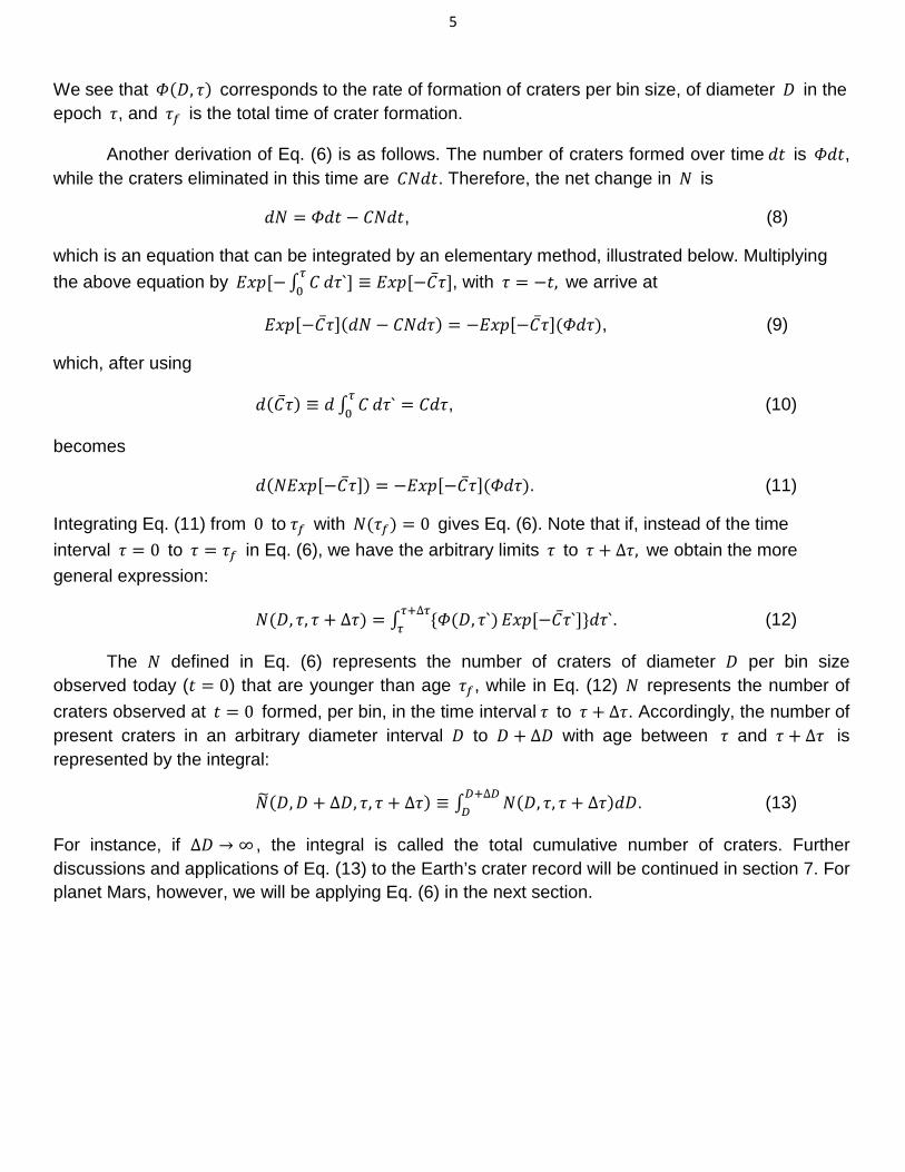
We see from Eq. (19) that a numerical calculation of 𝛷� for Mars requires an estimate of 𝜏𝑓, so with that goal we write:

𝜏𝑓=3.55103

𝛽𝑚𝑦, (56)

where 𝛽 is a number close to 1. For example, the range of values 3000my < 𝜏𝑓 < 4000my is covered by ~0.9 < 𝛽 < ~1.2. Hence, using Eq. (56) in Eq. (19), we obtain:

𝛷� = 𝛽106

𝐷4.3 (𝑚𝑦)−1, (57)

and thus the cumulative rate is:

𝛷�𝐶(Mars)= 𝛽106

3.3𝐷3.3 (𝑚𝑦)−1. (58)

For instance, for 𝐷 = 20𝑘𝑚 we obtain:

𝛷𝐶(Mars,20𝑘𝑚)≅ 15𝛽𝑚𝑦

≈ 15𝑚𝑦

, (59)

which implies that the cumulative flux per area is, with 𝑅𝑚 being the Martian radius,

15/(4𝜋𝑅𝑚2)𝑚𝑦

≅ 100×10−9

(𝑚𝑦)𝑘𝑚2 . (60)

The above results are considerably higher than the values for Earth from Eq. (47) and the results of Grieve and Shoemaker (1994) that are respectively :

2.8[1∓0.50𝑚𝑦

] , (61)

(5.5∓2.7)10−9

(𝑚𝑦)𝑘𝑚2 . (62)

Furthermore, for 𝐷 = 1𝑘𝑚, or, equivalently, impactor energies of around 1 to 2 megatons, we have, using Eq. (58),

𝛷�𝐶(Mars, 1𝑘𝑚)= 𝛽3.3𝑦

≈ 13.3𝑦

. (63)

It is not surprising that the impact rate on Mars is larger than that on Earth, because of Mars’ proximity to the asteroid belt; however, this shows that future Mars astronauts may have to deal with frequent damaging meteorite collisions. In particular, from the results above, we expect that Mars visitors spending a few years there will have a high probability of witnessing a megaton-type meteorite impact. Moreover, these impacts are likely to cause more damage on the surface than on our planet, due to the much lower atmospheric Martian density.

15

7. Application of the Model to Earth’s Cumulative Crater Number-Size Distribution

Our model predicts, in accordance with Eqs. (13) and (12), that the number of craters with diameters between 𝐷𝑖 and 𝐷𝑓 and ages between 𝜏𝑖 and 𝜏𝑓 is given by the expression:

𝑁� ≡ ∫ 𝑑𝐷 ∫ 𝛷{𝐸𝑥𝑝[−𝐶̅𝜏]}𝑑𝜏𝜏𝑓𝜏𝑖

𝐷𝑓𝐷𝑖

. (64)

Furthermore, assuming that:

𝛷 = 𝐴𝑟 𝐷𝑚

, (65)

𝐶̅ = 𝐵𝐷𝑝

, (66)

we obtain from Eq. (64), as shown in Appendix D,

𝑁�= 𝐴𝑟𝑝𝐵

(𝐵𝜏𝑖)−𝑛{𝛤[𝑛, 𝐵𝜏𝑖𝐷𝑓𝑝 , 𝐵𝜏𝑖

𝐷𝑖𝑝 ]-( 𝜏𝑖

𝜏𝑓)𝑛𝛤[𝑛, 𝐵𝜏𝑓

𝐷𝑓𝑝 , 𝐵𝜏𝑓

𝐷𝑖𝑝 ]}, (67)

where:

𝛤[𝑛, 𝑥,𝑦] ≡ ∫ 𝑥𝑛−1𝑦𝑥 𝑒−𝑥𝑑𝑥, (68)

is the generalized incomplete Gamma function, and:

𝑛 ≡ 𝑚−𝑝−1𝑝

. (69)

The above equation for 𝑁� contains the parameters 𝑚,𝑝,𝐵 , and the amplitude 𝐴𝑟 which will be defined more precisely below. The values to be used for 𝑚 and 𝑝 are those determined for Mars, since this is strongly suggested by our previous arguments, observations and interpretation of the model. Also, we will write:

𝐵 = 12𝑏1𝑚𝑦

, (70)

where 𝑏1 is a parameter that allows for the uncertainties in the value of 𝐵, which was determined, by the graphs in Figures (3) and (4), to be approximately:

𝐵(𝑔 = 0.5) ≅ 11𝑚𝑦

, (71)

𝐵(𝑔 = 0.1) ≅ 12𝑚𝑦

, (72)

where 𝑔 ≡ 𝜏𝐿 𝜏𝑅� . Furthermore, 𝐴𝑟 is defined by:

𝛷𝑟 = 𝐴𝑟 𝐷𝑚

, (73)

where 𝛷𝑟 is the flux of impacts on the Earth’s surface chosen for the application of Eq. (67). In order to reduce the uncertainties due to undercounting in the crater data we will select the following regions for this study:

16

(a) Continental United States (b) Canada up to the Arctic Circle latitude (c) Europe (d) Australia

The above area is considered to have well-counted crater data, particularly for 𝐷 >20𝑘𝑚. 𝐴𝑟 is then the reduced flux amplitude corresponding to this region, which is proportional to the fraction of our planet covered by the above area, and thus we have:

𝐴𝑟 = 𝐴 𝐴𝑟𝑒𝑎 𝑈𝑛𝑑𝑒𝑟 𝐶𝑜𝑛𝑠𝑖𝑑𝑒𝑟𝑎𝑡𝑖𝑜𝑛𝐸𝑎𝑟𝑡ℎ`𝑠 𝑆𝑢𝑟𝑓𝑎𝑐𝑒 𝐴𝑟𝑒𝑎

, (74)

where 𝐴 is given, from Eq. (48), by:

𝐴 = (1.82)105[1 ∓ 0.5]/𝑚𝑦. (75)

The crater data is taken from The Planetary and Space Science Centre. The area under consideration is approximately 30 million 𝑘𝑚2, with an uncertainty well below that of 𝐴 so that we can write:

𝐴𝑟 ≅ 𝐴(5.910−2) = (1.07)104𝑎1, (76)

where 𝑎1 represents the uncertainties in 𝐴𝑟, and is approximately given by:

𝑎1 ≅ [1 ∓ 0.5]/𝑚𝑦. (77)

Therefore we can write the theoretical 𝑁� with no free parameters, except for the uncertainties in 𝐴𝑟 and 𝐵 that are reflected in 𝑎1 and 𝑏1. We do this first in Table III and Figure (5) for craters with 𝐷 ≥ 20𝑘𝑚 and cumulative age starting with 𝜏 = 1𝑚𝑦 up to 𝜏 = 2,000𝑚𝑦 . Furthermore, we put 𝜏𝑓 = 2,500𝑚𝑦 and 𝐷𝑓 = 300𝑘𝑚, since all craters in the field of study are within this bin size. This theoretical curve, 𝑁�(𝜏) , is compared with the corresponding observational data, allowing a Mathematica program to do a fitting only on the values of 𝑎1 and 𝑏1. The values of 𝑎1 and 𝑏1 arising from this best fitting are 𝑎1 = 0.80/𝑚𝑦 and 𝑏1 = 1.68 , which are within the expected uncertainties, and the very good agreement between theory and observations is noteworthy.

On the other hand, we also compared theory and observation in Table IV and Figure (6), where now 𝑁� accumulative represents the number of craters of all ages, 1𝑚𝑦 ≤ 𝜏 ≤ 2,500, with diameters greater than or equal to 𝐷. Again, the theoretical 𝑁�(𝐷) is in very good agreement with the observations for 𝐷 ≥ ~20𝑘𝑚, although not so good for 𝐷 ≤ ~20𝑘𝑚, which is as expected due to the undercounting, which has already been mentioned, of craters of these sizes. Note that the slope of these accumulative curves is a function of 𝐷 , and therefore it is not simply characterized by exponents as was the case in Figure (2) for Mars.

Perhaps it should be remarked that, in order to understand the similarities between theory and observation for the Earth’s crater data when considering very low numbers of craters, a probabilistic approach to our model predictions is necessary. This statistical view could be similar to how the results of opinion polls are justified when based on only a small fraction of the total population: if the

17

small sample of the poll is a well-chosen representative of the whole, then the errors remain low.

FIGURE (5): 𝐿𝑜𝑔[𝑁]�𝑣𝑠𝐿𝑜𝑔[𝜏 ≡ 𝐴𝑔𝑒], for all Diameters 𝐷 ≥ 20𝑘𝑚. See Table III.

Table III

𝜏(𝑚𝑦) 𝑁�[𝜏,𝐷 ≥ 20𝑘𝑚 ] Observation

1 33.14 33

10 32.00 32

20 30.80 31

40 28.62 29

50 27.62 28

100 23.40 24

150 20.24 20

200 17.80 17

300 14.20 13

400 11.70 10

600 8.50 8

800 6.50 5

1000 5.00 5

1200 3.89 4

1400 2.99 3

1600 2.25 3

1800 1.62 2

2000 1.08 1

18

FIGURE (6): [𝐿𝑜𝑔[𝑁�] vs 𝐿𝑜𝑔[𝐷 ≡ 𝐷𝐴𝑐𝑐], for all ages between 1𝑚𝑦 ≤ 𝜏 ≤ 2,500𝑚𝑦. See Table IV below.

Table IV

𝐷 𝑁�[𝐷, 1𝑚𝑦 ≤ 𝜏 ≤ 2,500𝑚𝑦 ] Observation

1 166.00 121

2 165.00 118

4 137.00 99

8 82.60 72

16 42.40 37

20 33.14 33

32 18.18 16

45 10.37 10

64 4.79 5

91 1.82 2

128 0.62 1

19

Appendix A

Consider the following initial way of writing 𝑁(𝐷) (see Appendix B):

𝑁 = (𝛷/𝐶������){1− 𝐸𝑥𝑝[−�̅�𝜏]}, A.1

where

(𝛷/𝐶������) ≡ ∫ (𝛷(𝜏`)/𝐶){Exp[−∫ 𝐶(𝜏``)𝑑𝜏``]}𝐶𝑑𝜏`𝜏`0

𝜏0

∫ {𝐸𝑥𝑝[−∫ 𝐶(𝜏``)𝑑𝜏``]}𝐶𝑑𝜏`𝜏`0

𝜏0

, A.2

�̅� ≡ ∫ 𝐶𝑑𝜏`𝜏0𝜏

. A.3

We note that �̅� is the time average of 𝐶 and (𝛷/𝐶������) is the weighted average of 𝛷/𝐶, with weight:

∫ {𝐸𝑥𝑝[−∫ 𝐶(𝜏``)𝑑𝜏``]}𝐶𝑑𝜏`𝜏`0

𝜏0 . A.4

From physical considerations we expect that, in the limits 𝐷 → ∞ (𝐷 → 0), we will have �̅� → 0 (�̅� → ∞), and therefore, from Eq. (A.1), with 𝜏 = 𝜏𝑓, we see that:

𝑁 → (𝛷/𝐶������)�̅�𝜏𝑓, 𝐷 → ∞, 𝐶� → 0, A.5

𝑁 → (𝛷/𝐶������) , 𝐷 → 0, 𝐶� → ∞. A.6

On the other hand, we also know that in the limit 𝐷 → ∞, �̅� → 0 craters are conserved, and consequently

𝑁 = ∫ 𝛷𝜏𝑓0 d𝜏 ≡ 𝛷�𝜏𝑓, 𝐷 → ∞, �̅� → 0. A.7

Hence, comparing Eq. (A.5) with Eq. (A.7), we obtain:

(𝛷/𝐶������) = 𝛷�

�̅� 𝐷 → ∞, �̅� → 0. A.8

Moreover, in the limit 𝐷 → 0, �̅� → ∞, we expect that the rate of production, 𝛷, is equal to the rate of elimination, 𝑁𝐶, hence, keeping 𝑁 constant (i.e. saturation), and we thus have

𝛷 = 𝑁𝐶; 𝐷 → 0, �̅� → ∞, A.9

or, since 𝑁 is now constant,

𝑁 = 𝛷�

�̅�; 𝐷 → 0, �̅� → ∞. A.10

Comparing Eq. (A.10) with Eq. (A.6) we again obtain:

(𝛷/𝐶������) = 𝛷�

�̅�, 𝐷 → 0, �̅� → ∞. A.11

Therefore we have shown in Eqs. (A.8) and (A.11) that:

(𝛷/𝐶������) = 𝛷�

�̅�, 𝐷 → 0 𝑜𝑟 𝐷 → ∞. A.12

20

Although the identification in Eq. (A.12) is only in the limits 𝐷 → 0 𝑜𝑟 𝐷 → ∞, this however corresponds to the part of the crater data that is described respectively by the two straight lines in Eqs. (27) and (25) and in the log-log plot in Figure (2), which essentially comprise all data points.

21

Appendix B

We are going to show that the equation:

𝑁 = ∫ 𝛷(𝜏`){𝐸𝑥𝑝[−∫ 𝐶(𝜏``)𝑑𝜏``]}𝑑𝜏`𝜏`0

𝜏0 , B.1

can be written as Eq. (A.1):

𝑁 = (𝛷/𝐶������){1− 𝐸𝑥𝑝[−𝐶̅𝜏]}. B.2

where

(𝛷/𝐶������) ≡ ∫ (𝛷(𝜏`)/𝐶){𝐸𝑥𝑝[−∫ 𝐶(𝜏``)𝑑𝜏``]}𝐶𝑑𝜏`𝜏`0

𝜏0

∫ {𝐸𝑥𝑝[−∫ 𝐶(𝜏``)𝑑𝜏``]}𝐶𝑑𝜏`𝜏`0

𝜏0

. B.3

𝐶̅ ≡ ∫ 𝐶𝑑𝜏`𝜏0𝜏

. B.4

Note that 𝐶̅ is the time average of 𝐶 and (𝛷/𝐶������) is the weighted average of 𝛷/𝐶, with weight:

∫ {𝐸𝑥𝑝[−∫ 𝐶(𝜏``)𝑑𝜏``]}𝐶𝑑𝜏`𝜏`0

𝜏0 . B.5

First, by equating Eq. (B.1) to Eq. (B.2) and using Eq. (B.3), we see that the demonstration is equivalent to showing that:

∫ {𝐸𝑥𝑝[−∫ 𝐶(𝜏``)dτ``]}𝐶𝑑𝜏`𝜏`0

𝜏0 = {1 − 𝐸𝑥𝑝[− 𝐶 �𝜏 ] }. B.6

To this end, consider the elementary integral:

∫ 𝑒−𝑦` 𝑑𝑦` = 1 − 𝑒−𝑦𝑦0 , B.7

so that, if we define

𝑦` ≡ ∫ Cdτ``𝜏`0 , B.8

𝑑𝑦` = 𝐶(𝜏`)𝑑𝜏`, B.9

we obtain, substituting Eqs. (B.8) and (B.9) in Eq. (B.7),

∫ {𝐸𝑥𝑝[−∫ 𝐶(𝜏``)𝑑𝜏``]}𝐶𝑑𝜏`𝜏`0

𝜏0 = 1-𝐸𝑥𝑝[−∫ 𝐶𝑑𝜏` ]𝜏

0 , B.10

which, after using the definition in Eq. (B.4), is Eq. (B.6). QED.

22

Appendix C: Derivation of Equation (36)

The average of the diameters of craters of age 𝜏 ∓ ∆𝜏 observed today is given by:

𝐷� = ∫ 𝐷𝑁(𝐷,𝜏𝐿,𝜏𝑅)𝑑𝐷∞0

∫ 𝑁(𝐷,𝜏𝐿,𝜏𝑅)𝑑𝐷∞0

, C.1

where

𝑁(𝐷, 𝜏𝐿 , 𝜏𝑅) = ∫ 𝛷(𝐷, 𝜏)𝐸𝑥𝑝[−𝐶̅𝜏]𝑑𝜏𝜏𝑅𝜏𝐿

. C.2

If Ф and 𝐶̅ are independent of 𝜏, we have, after integrating Eq. (C.2):

𝑁(𝐷, 𝜏𝐿 , 𝜏𝑅) = Ф

𝐶̅(𝑒−𝐶̅𝜏𝐿 − 𝑒−𝐶̅𝜏𝑅), C.3

and furthermore if:

𝛷 = 𝐴𝐷𝑚

, C.4

𝐶̅ = 𝐵𝐷𝑝

, C.5

we obtain from Eq. (C.3):

𝑁(𝐷, 𝜏𝐿 , 𝜏𝑅) = 𝐴𝐵𝐷−𝑚`[𝑒−𝑥 − 𝑒−�̅�], C.6

where, with 𝑔 = 𝜏𝐿 𝜏𝑅� ,

𝑚` = 𝑚− 𝑝, C.7

𝑥 ≡ 𝐵𝜏𝐿𝐷𝑝

, �̅� ≡ 𝐵�𝜏𝐿𝐷𝑝

,𝐵� ≡ 𝐵𝑔

. C.8

Therefore, substituting Eq. (C.6) in Eq. (C.1) we obtain:

𝐷�=∫𝐷−𝑚`+1[𝑒−𝑥−𝑒−𝑥�]dD∞

0

∫ 𝐷−𝑚`[𝑒−𝑥−𝑒−𝑥�]dD∞0

. C.9

Now, we can write, for any constant 𝑘, (see Appendix D for details):

∫ D−ke−xdD∞0 = (𝐵𝜏𝐿)

1−𝑘𝑝

𝑝 ∫ 𝑥𝑘−1−𝑝

𝑝∞0 𝑒−𝑥𝑑𝑥, C.10

∫ 𝐷−𝑘𝑒−�̅�dD∞0 = (𝐵�𝜏𝐿)

1−𝑘𝑝

𝑝 ∫ �̅�𝑘−1−𝑝

𝑝∞0 𝑒−�̅�𝑑�̅�. C.11

23

However, we have that ∫ 𝑥𝑘−1−𝑝

𝑝∞0 𝑒−𝑥𝑑𝑥 = 𝛤 �𝑘−1

𝑝� = the complete Gamma Function, and

thus we obtain from Eq. (C.9), after using Eqs. (C.10) and (C.11),

𝐷�=((BτL)

2−m`p −(BτL/g)

2−m`p )Γ�m`−2

p �

((BτL)1−m`p −�BτL/g�

1−m`p )Γ�m`−1

p �=( 𝐵𝜏𝐿)

1𝑝𝛼1, C.12

where

𝛼1 = 𝛤((𝑚`−2) 𝑝)⁄𝛤((𝑚`−1) 𝑝)⁄

[1−𝑔(𝑚`−2) 𝑝⁄ ][1−𝑔(𝑚`−1) 𝑝⁄ ]

, C.13

thus arriving at Eq. (36).

24

Appendix D: Deriving Equation (67)

Consider Eq. (64)

𝑁� = ∫ (dD) 𝑁�𝐷, 𝜏𝑖, 𝜏𝑓�𝐷𝑓𝐷𝑖

≡ ∫ 𝑑𝐷 ∫ 𝛷{𝐸𝑥𝑝[−𝐶̅𝜏]}𝑑𝜏𝜏𝑓𝜏𝑖

𝐷𝑓𝐷𝑖

, D.1

and assume that:

𝛷 = 𝐴𝑟 𝐷𝑚

, D.2

𝐶̅ = 𝐵𝐷𝑝

, D.3

We then obtain, after integrating first with respect to 𝜏,

𝑁� = ∫ �𝐴𝑟𝐵𝐷−𝑚`[𝑒−𝑥 − 𝑒−�̅�] �dD,𝐷𝑓

𝐷𝑖 D.4

where:

𝑚` = 𝑚− 𝑝, D.5

𝑥 ≡ 𝐵𝜏𝑖𝐷𝑝

, �̅� ≡ 𝐵�𝜏𝑖𝐷𝑝

,𝐵� ≡ 𝐵𝑔. D.6

We now change the variable of integration in Eq. (D.4) from 𝐷 to 𝑥:

𝐷 = (𝐵𝜏𝑖𝑥

)1/𝑝, D.7

𝑑𝐷 = −(1𝑝

)(𝐵𝜏𝑖)1/𝑝𝑥−1−1/𝑝)𝑑𝑥, D.8

from which we obtain:

∫ 𝐷−𝑚`𝐷𝑓𝐷𝑖

𝐸𝑥𝑝[−𝑥]𝑑𝐷 = �1𝑝� (𝐵𝜏𝑖)(1−𝑚`)/𝑝 ∫ 𝑥

(𝑚`−1−𝑝𝑝𝑥𝑖

𝑥𝑓𝐸𝑥𝑝[−𝑥]𝑑𝑥 = �1

𝑝� (𝐵𝜏𝑖)−𝑛𝛤[𝑛, 𝑥𝑓,𝑥𝑖], D.9

Where

𝑛 = (𝑚` − 1)/𝑝, D.10

and we use the generalized Gamma function:

𝛤�𝑛, 𝑥𝑖,𝑥𝑓� = − 𝛤�𝑛, 𝑥𝑓,𝑥𝑖� ≡ ∫ 𝑥𝑛−1𝑥𝑓𝑥𝑖

𝐸𝑥𝑝[−𝑥]𝑑𝑥. D.11

Likewise, we also have:

∫ 𝐷−𝑚`𝐷𝑓𝐷𝑖

𝐸𝑥𝑝[−�̅�]𝑑𝐷 = �1𝑝� (𝐵�𝜏𝑖)−𝑛𝛤[𝑛, �̅�𝑓 , �̅�𝑖]. D.12

25

Note that if 𝐷𝑖 = 0 and 𝐷𝑓 = ∞ then 𝑥𝑖 = ∞ and 𝑥𝑓 = 0, and if we identify 𝑚` with 𝑘 in Eqs. (C.10) and (C.11), then Eqs. (D.9) and (D.12) become Eqs. (C.10) and (C.11). Substituting Eqs. (D.9) and (D.12) in Eq. (D.4), we find that:

𝑁� = 𝐴𝑟𝐵𝑝

{(𝐵𝜏𝑖)−𝑛𝛤�𝑛, 𝑥𝑓,𝑥𝑖� -(𝐵�𝜏𝑖)−𝑛𝛤[𝑛, �̅�𝑓 , �̅�𝑖]} . D.13

Thereby, with Eq. (D.6) and some algebra, we find the result in Eq. (67):

𝑁�= 𝐴𝑟𝑝𝐵

(𝐵𝜏𝑖)−𝑛{𝛤[𝑛, 𝐵𝜏𝑖𝐷𝑓𝑝 , 𝐵𝜏𝑖

𝐷𝑖𝑝 ]-( 𝜏𝑖

𝜏𝑓)𝑛𝛤[𝑛, 𝐵𝜏𝑓

𝐷𝑓𝑝 , 𝐵𝜏𝑓

𝐷𝑖𝑝 ]}. D.14

26

References

1. Barlow, N.G. (1988) Icarus, 75, 285.

2. Garvin, J.B. (2002) Lunar and Planetary Science XXXIII, 1255.

3. Poveda, A., Herrera, M.A. Garcia, J.L., Curioca, K. (1999) Planetary and Space Science, 47, 679-685. I

4. Hartmann, W.K. ( 2002) Lunar and Planetary Science XXXIII, 1876.

5. Hartmann, W.K. (1966) Icarus, 5, 406.

6. Neukum, G. et al. (2001) Chronology and Evolution of Mars 55 Bern: International Space Science Institute.

7. Neukum, G. (1983) Ludwig-Maximillians-University Munich, 186.

8. Ryder, G. (1990) EOS, 71, 313.

9. Grieve and Shoemaker, (1994) The Record of Past Impacts on Earth. In: “Hazards Due To Comets And Asteroids, T. Gehrels, Editor, The University Of Arizona Press.

10. Gault, D.E. (1974) In “Impact Cratering”, Greeley R. and Schultz P. (Eds.),A Primer In Lunar Geology, Ames Research , NASA, p 247-275.

11. Holsapple, K.A.(1987). Int J. Impact Eng., 5,343.

12. Schmidt, R. M. and Housen K.R.(1987), Int. J. Impact Eng., 5,543.

13. Melosh,H. J.(1989). Impact Cratering, A geological Process. Oxford Univ. Press.NY.

14. Hughes, D.W. (1998), Meteorites: Flux with Time and Impact Effects, Edited by Grady, M.M., Hutchison, R., McCall, G.J. and Rothery, D.A. Geological Society Special Publication No. 140.

15. Ward, S.N. (2002) Planetary Cratering: A Probabilistic Approach; Journal of Geophysical Research, Volume 107, No. E4.

16. Silber, E.A., Revelle, D.O., Brown, P.G., Edwards, W.N. (2009) Journal of Geophysical Research, Vol.114, E08006.

17. Lewis, J.S. (1996) Book “Rain Of Iron And Ice”,p 124, Addison-Wesley Publishing Company

18. Asher, D.J., Bailey, E.V., Napier, B. (2005) “Earth In The Cosmic Shooting Gallery”, Observatory,125, p 319-322.

19. The Planetary and Space Science Centre(PASSC), Earth Impact Database (http://www.passc.net/EarthImpactDatabase/)