Preliminary Manual of the software program Multidimensional Item

Response Theory (MIRT) July 7th, 2010

Cees A. W. Glas Department of Research Methodology, Measurement, and Data Analysis Faculty of Behavioural Science, University of Twente P.O. Box 217 7500 AE Enschede, the Netherlands Phone +31 53 489 35 65 Private +31 53 430 68 13 Fax +31 53 489 42 39 Mobile 06 307 409 52

1. Introduction

2. The model

2.1 Models for Dichotomous data

2.1.1. The Rasch model

2.1.2 Two- and three-parameter models

2.2 Models for Polytomous Items

2.2.1 Introduction

2.2.2 Adjacent-category models

2.2.3 Continuation-ratio models

2.2.4 Cumulative probability models

2.4 Multidimensional Models

3. Data collection designs

4. Scope of the program as released

5. The structure of the data file

6. Running the program

6.1. Introduction

6.2. The General screen

6.3. The Tests screen

6.4. The Options screen

6.5. The priors screen

6.6. The Item Fit screen

6.8. The Person Fit screen

6.9. The Criteria screen

6.10. The Criteria Mirt screen

6.11. The Advanced screen

6.12. Starting the Computations and viewing the output

7. The Output

7.1. The file JOPBNAME.MIR

7.2. The file JOPBNAME.WRM1 and JOPBNAME.WRM2

7.3. The file JOPBNAME.PRS1 and JOPBNAME.PRS2

7.4. The file JOPBNAME.EAP1 and JOPBNAME.EAP2

Bibliography

1. Introduction

Item response theory (IRT) provides a useful and theoretically well-founded framework for

educational measurement. It supports such activities as the construction of measurement instruments,

linking and equating measurements, and evaluation of test bias and differential item functioning.

Further, IRT has provides the underpinnings for item banking, optimal test construction and various

flexible test administration designs, such as multiple matrix sampling, flexi-level testing and

computerized adaptive testing.

The MIRT package supports the following models:

• The Rasch model for dichotomous data (1PLM, Rasch, 1960),

• The OPLM model for dichotomous and polytomous data (Verhelst & Glas, 1995),

• The two- and three-parameter logistic models and the two- and three-parameter normal ogive

models (2PLM, 3PLM, 2PNO, 3PNO, Lord & Novick, 1968, Birnbaum, 1968) for

dichotomous data,

• The partial credit model (PCM, Masters, 1982),

• The generalized partial credit model (GPCM, Muraki, 1992),

• The sequential model (SM, Tutz, 1990),

• The graded response model (GRM, Samejima, 1969),

• The nominal response model (NRM, Bock, 1972).

• Generalizations of these models to models with between-items multidimensionality.

The MIRT package supports the following statistical procedures:

• CML estimation of the item parameters of the 1PLM, the PCM and the OPLM,

• MML estimation of the item and population parameters,

• MCMC estimation of the item, person and population parameters

• ML and WML estimation of person parameters,

• EAP estimation of person parameters,

• Item fit analysis,

• Analysis of differential item functioning,

• Person fit analysis.

2. The model

2.1 Models for Dichotomous data

2.1.1. The Rasch model

In this section, the focus is on dichotomous data. A response of a student i to an item k will be

coded by a stochastic variable Yik. In the sequel, upper-case characters will denote stochastic

variables. The realizations will be lower case characters. In the present case, there are two possible

realizations, defined by

1 if person responded correctly to item

0 if this is not the case. iki k

y

= (1)

MIRT supports the case where not all students responded to all items. To indicate whether a

response is available, we define a variable

1 if a response of person to item is available

0 if this is not the case. ik

i kd

=

(2)

It will be assumed that the values are a-priori fixed by some test administrator. Therefore, dik can be

called a test administration variable. We will not consider dik as a stochastic variable, that is, the

estimation and testing procedure will be explained conditionally on dik, that is, with dik fixed. Later,

this assumption will be broadened.

In an incomplete design, the definition of the response variable Yik is generalized such that it

assumes an arbitrary constant if no response is available.

The simplest model, where every student is represented by one ability parameter and every item is

represented by one difficulty parameter, is the 1-parameter logistic model, better known as the Rasch

model (Rasch, 1960). It is abbreviated as 1PLM. It is a special case of the general logistic regression

model. This also holds for the other IRT models discussed below. Therefore, it proves convenient to

first define the logistic function:

exp( ) ( ) 1 exp( )

xxx

Ψ =+

The 1PLM is then defined as

( 1| , ) ( )ik i k i kp Y b bθ θ= = Ψ − (3)

that is, the probability of a correct response is given by a logistic function with argument θi - bk.

Note that the argument has the same linear form as in Formula (1). Using the abbreviation

( ) ( 1 | , )k i kP p Y bθ θ= = , the two previous formulas can be combined to

exp( ) ( ) 1 exp( )

i kk i

i k

bPb

θθ

θ−

=+ −

(4)

The probability of a correct response as a function of ability, ( )kP θ , is the so-called item response

function of item k. Two examples of the associated item response curves are given in Figure 2.1. The

x-axis is the ability continuumθ. For two items, with distinct values of bk, the probability of a correct

response ( )kbθΨ − is plotted for different values of θ. The item response curves increase with the

value of θ, so this parameter can be interpreted as an ability parameter. Note that the order of the

probabilities of a correct response for the two items is the same for all ability levels.

Figure 2.1 Response curves for two items in the Rasch model.

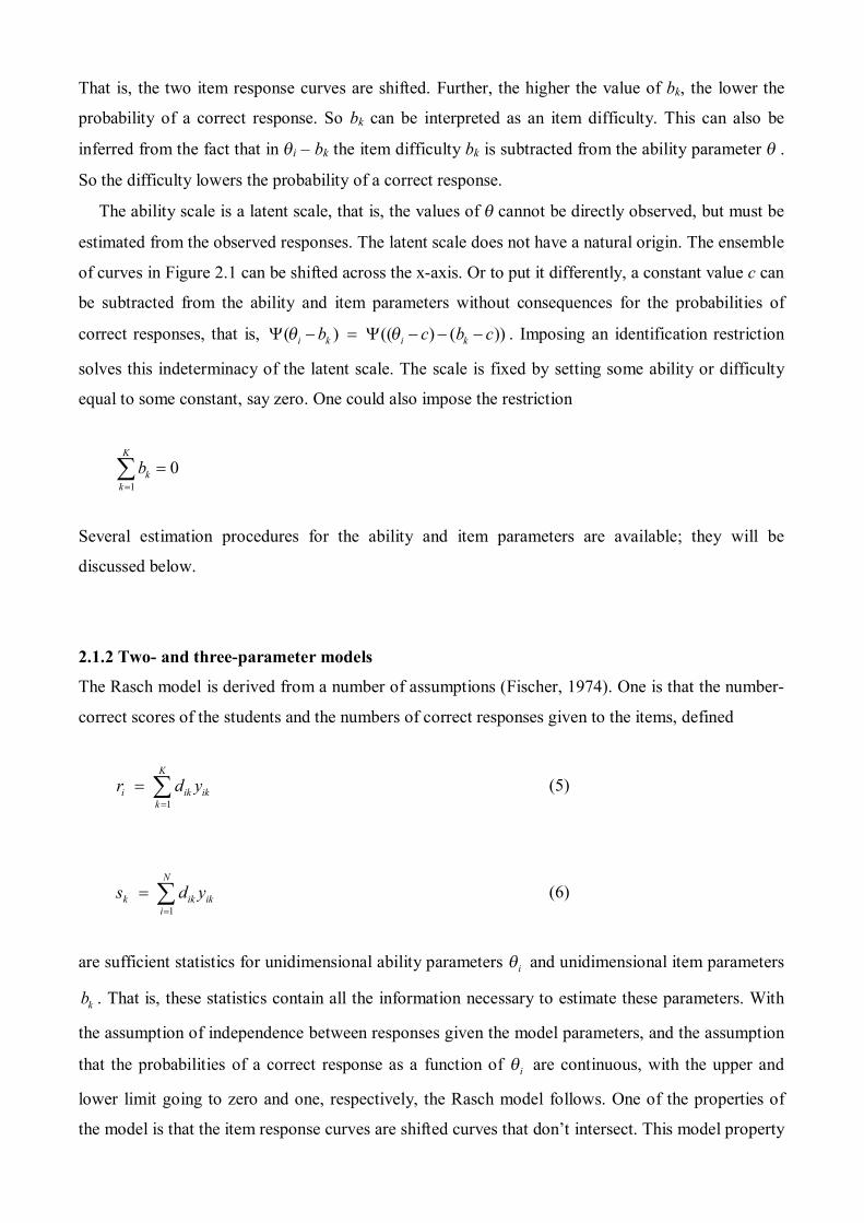
That is, the two item response curves are shifted. Further, the higher the value of bk, the lower the

probability of a correct response. So bk can be interpreted as an item difficulty. This can also be

inferred from the fact that in θi – bk the item difficulty bk is subtracted from the ability parameter θ .

So the difficulty lowers the probability of a correct response.

The ability scale is a latent scale, that is, the values of θ cannot be directly observed, but must be

estimated from the observed responses. The latent scale does not have a natural origin. The ensemble

of curves in Figure 2.1 can be shifted across the x-axis. Or to put it differently, a constant value c can

be subtracted from the ability and item parameters without consequences for the probabilities of

correct responses, that is, ( ) (( ) ( ))i k i kb c b cθ θΨ − = Ψ − − − . Imposing an identification restriction

solves this indeterminacy of the latent scale. The scale is fixed by setting some ability or difficulty

equal to some constant, say zero. One could also impose the restriction

1

0K

kk

b=

=∑

Several estimation procedures for the ability and item parameters are available; they will be

discussed below.

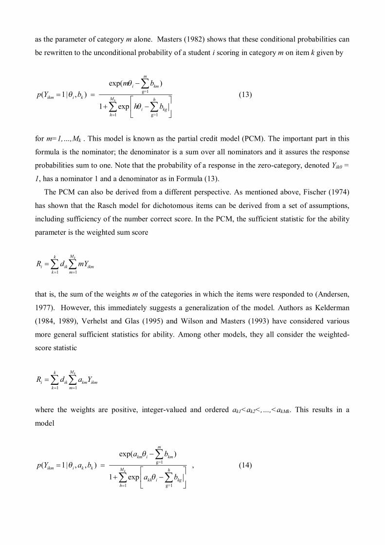
2.1.2 Two- and three-parameter models

The Rasch model is derived from a number of assumptions (Fischer, 1974). One is that the number-

correct scores of the students and the numbers of correct responses given to the items, defined

1

K

i ik ikk

r d y=

= ∑ (5)

1

N

k ik iki

s d y=

= ∑ (6)

are sufficient statistics for unidimensional ability parameters iθ and unidimensional item parameters

kb . That is, these statistics contain all the information necessary to estimate these parameters. With

the assumption of independence between responses given the model parameters, and the assumption

that the probabilities of a correct response as a function of iθ are continuous, with the upper and

lower limit going to zero and one, respectively, the Rasch model follows. One of the properties of

the model is that the item response curves are shifted curves that don’t intersect. This model property

may not be appropriate. Firstly, the nonintersecting response curves impose a pattern on the

expectations that may be insufficiently reflected in the observations, so that the model is empirically

rejected because the observed responses and their expectations don’t match. That is, it may be more

probable that the response curves actually do cross. Secondly, on theoretical grounds, the zero lower

asymptote (the fact that the probability of a correct response goes to zero for extremely low ability

levels) may be a misspecification because the data are responses to multiple-choice items, so even at

very low ability levels the probability of a correct response is still equal to the guessing probability.

To model these data, a more flexible response model with more parameters is needed. This is found

in the 2-, and 3-parameter logistic models (2PLM and 3PLM, Birnbaum, 1968). In the 3PLM, the

probability of a correct response, depends on three item parameters, ,ka ,kb and kc , which are called

the discrimination, difficulty and guessing parameter, respectively. The model is given by

( ) (1 ) ( ( ))

exp( ( ))(1 )1 exp( ( ))

k i k k k i k

k i kk k

k i k

P c c a b

a bc ca b

θ θ

θθ

= + − + Ψ −

−= + −

+ −

(7)

The 2PLM follows by setting the guessing parameter equal to zero, so upon introducing the

constraint 0kc = and the 1PLM follows upon introducing the additional constraint 1ka = .

Figure 2.2 Response curves for two items in the 2PLM.

Two examples of response curves of the 2PLM are shown in the Figure 2.2. It can be seen that under

the 2PLM the response curves can cross. The parameter ka determines the steepness of the response

curve: The higher ka , the steeper the response curve. The parameter ka is called the discrimination

parameter because it indexes the dependence of the item response on the latent variable θ . This can

be seen as follows. Suppose the 2PLM holds and 0ka = . Then the probability of a correct response

is equal to

exp(0) 1 (0)1 exp(0) 2

Ψ = =+

That is, the probability of a correct response is equal to a half for all values of the ability variable θ,

so the response does not depend on θ. If, on the other hand, the discrimination parameter ka goes to

infinity, the item response curve becomes a step function: the probability of a correct response goes

to zero if kbθ < and it goes to one if kbθ > . So this item distinguishes between respondents with an

ability value θ below or above the item difficulty parameter kb . As in the 1PLM, the difficulty

parameter kb still determines the position of the response curve: if kb increases, the response curve

moves to the right and the probability of a correct response for a given ability level θ decreases, that

is, the item becomes more difficult.

An item response curve for the 3PLM is given in Figure 2.3. The value of the guessing parameter

was equal to 0.20, that is, 0.20kc = . As a result, the lower asymptote of the response curve goes to

0.20 instead of to zero, as in the 2PLM. So the probability of a correct response of students with a

very low ability level is still equal to the guessing probability, in this case, to 0.20.

Figure 2.3 Response curve for an item in the 3PLM

Above it was mentioned that the 1PLM can be derived from a set of assumptions. On of these was

the assumption that the number-correct scores given by Formula (5) are sufficient statistics for the

ability parameters. Birnbaum (1968) has shown that the 2PLM can be derived from the same set of

assumptions, with the difference that it is now assumed that the weighted sum score

1

K

i ik k ikk

r d a y=

= ∑ (8)

is a sufficient statistic for ability. Note that the correct responses are now weighted with the

discrimination parameters ak. Since ri is assumed to be a sufficient statistic, the weights ak should be

known constants. Usually, however, the weights ak are treated as unknown parameters that must be

estimated. The two approaches lead to different estimation procedures, which will be discussed in

the next section.

It should be noted that the first formulations of IRT did not use the logistic function but the

normal ogive function (Lawley, 1943, 1944; Lord, 1952, 1953a and 1953b). The normal ogive

function ( )xΦ is the probability mass under the standard normal density function left of x. With a

proper transformation of the argument, ( ) (1.7 )x xΦ = Ψ , the logistic and normal ogive curves are

very close, and indistinguishable for all practical work. Therefore, the 3PNO, given by

( ) (1 ) ( ( )) k i k k k i kP c c a bθ θ= + − + Φ − (9)

is equivalent with the 3PLM for al practical purposes. The statistical framework used for parameter

estimation often determines the choice between the two formulations.

The final remark of this section pertains to the choice between the 1PLM on one hand and the

2PLM and the 3PLM on the other. The 1PLM can be mathematically derived from a set of

measurement desiderata. Its advocates (Rasch, 1960, Fischer, 1974, Wright & Stone, 1979) show

that the model can be derived from the so-called requirement of specific objectivity. Loosely

speaking, this requirement entails invariant item ordering for all relevant subpopulations. The 2PLM

and 3PLM, on the other hand, are an attempt to model the response process. Therefore, the 1PLM

may play an important role in psychological research, where items can be selected to measure some

theoretical construct. In educational research, however, the items and the data are given and items

cannot be discarded for the sake of model fit. There, the role of the measurement expert is to find a

model that is acceptable for making inferences about the students’ proficiencies and to attach some

measure of the reliability to these inferences. And though the 2PLM and the 3PLM are rather crude

as response process models, they are flexible enough to fit most data emerging in educational testing

adequately.

2.2 Models for Polytomous Items

2.2.1 Introduction

The present chapter started with an example of parameter separation where the responses to the

items were polytomous, that is, in the example of Table 2.1 the responses to the items are scored

between 0 and 5. Dichotomous scoring is a special case where the item scores are either 0 or 1.

Open-ended questions and performance tasks are often scored polytomously. They are usually

intended to be accessible to a wide range of abilities and to differentiate among test takers on the

basis of their levels of response. Response categories for each item capture this response diversity

and thus provide the basis for the qualitative mapping of measurement variables and the consequent

interpretation of ability estimates. For items with more than two response categories, however, the

mapping of response categories on to measurement variables is a little less straightforward than for

right/wrong scoring.

In the sequel, the response to an item k can be in one of the categories m=0,…,Mk. So it will be

assumed that every item has a unique number of response categories 1+Mk. The response of a

student i to an item k will be coded by stochastic variables Yikm. As above, upper-case characters will

denote stochastic variables, the analogous lower-case characters the realizations. So

1 if person responded in category on item 0 if this is not the case, ikm

i m ky

=

(10)

for m = 0,…,Mk. A dichotomous item is the special case where Mk = 1, and the number of response

variables is then equal to two. However, the two response variables Yik0 and Yik1 are completely

dependent, if one of them is equal to 1, the other must be equal to zero. For dichotomous items, a

response function was defined as the probability of a correct response as a function of the ability

parameter θ. In the present formulation, we define an item-category function as the probability of

scoring in a certain category of the item as a function of the ability parameter θ.

For a dichotomous item, we have two response functions, one for the incorrect response and one

for the correct response. However, as with the response variables also the response functions are

dependent because the probabilities of the different possible responses must sum to one, both for the

dichotomous case (Mk = 1) and for the polytomous case (Mk > 1). The generalization of IRT models

for dichotomous responses to IRT models for polytomous responses can be made from several

perspectives, several of which will be discussed below. A very simple perspective is that the

response functions should reflect a plausible relation with the ability variable. For assessment data,

the response categories are generally ordered, that is, a response in a higher category reflects a

higher ability level than a response in a lower category. However, items with nominal response

categories may also play a role in evaluation; therefore they will be discussed later. Consider the

response curves of a polytomous item with 5 ordered response categories given in Figure 2.5. The

response curve of a response in the zero-category decreases as a function of ability. This is plausible,

because as ability increases, the score of a respondent will probably be in a category m > 0. Further,

respondents of extremely low proficiency will attain the lowest score almost with a probability one.

An analogous argument holds for the highest category: this curve increases in ability, and for very

proficient respondents the probability of obtaining the highest possible score goes to one. These two

curves are in accordance with the models for dichotomous items discussed in the previous sections.

The response curves for the intermediate categories are motivated by the fact that they should have a

lower zero asymptote because respondents of very low ability almost surely score in category zero,

and respondents of very high ability almost surely score in the highest category. The fact that the

curves of the intermediate categories are single-peaked has no special motivation but most models

below have this property.

Figure 2.5. Response curves of a polytomously scored item.

Item response models giving rise to sets of item-category curves with the properties sketched here

fall into three classes (Mellenbergh, 1995). Models in the first class are called adjacent-category

models (Masters, 1982, Muraki, 1992), models in the second class are called continuation-ratio

models (Tutz, 1990, Verhelst, Glas, & de Vries, 1997) and models in the third class are called

cumulative probability models (Samejima, 1969). These models will be discussed in turn. It should,

however, be stressed in advance, that though the rationales underlying the models are very different,

the practical implications are often negligible, because their item-category response curves are so

close that they can hardly be distinguished in the basis of empirical data (Verhelst, Glas, & de Vries,

1997). On one hand, this is unfortunate, because the models represent substantially different

response processes; on the other hand, this is also convenient, because statisticians can choose a

model formulation that supports the most practical estimation and testing procedure. In this sense,

the situation is as in the case of models for dichotomous data where one can either choose a logistic

or normal ogive formulation without much consequence for model fit, but with important

consequences for the feasibility of the estimation and testing procedures. Finally, it should be

remarked that logistic and normal ogive formulations also apply within the three classes of models

for polytomous items, so one is left with a broad choice of possible approaches to modeling,

estimation and testing.

2.2.2 Adjacent-category models

In Section 2.1.1, the Rasch model or 1PLM was defined by specifying the probability of a correct

response. However, because only two response categories are present and the probabilities of

responding in either one of the categories sum to one, Formula (4) could also be written as

( 1| , ) exp( ) ( 0 | , ) ( 1| , ) 1 exp( )

ik i k i k

ik i k ik i k i k

p Y b bp Y b p Y b b

θ θθ θ θ

= −=

= + = + − (11)

that is, the logistic function ( )i kbθΨ − describes the probability of scoring in the correct category

rather than in the incorrect category. Formula (11) defines a conditional probability. The difficulty of

item k, bk, is now defined as the location on the latent θ scale at which a correct score is as likely as

an incorrect score.

Masters (1982) extends this logic to items with more than two response categories. For an item with

three ordered categories scored 0, 1 and 2, a score of 1 is not expected to be increasingly likely with

increasing ability because, beyond some point, a score of 1 should become less likely because a

score of 2 becomes a more probable result. It follows from the intended order 0<1<2,...,<mk of a set

of categories that the conditional probability of scoring in m rather than in m-1 should increase

monotonically throughout the ability range. The probability of scoring in in m rather than in m-1 is

thus modeled as

( 1)

( 1| , ) exp( ) ( 1| , ) ( 1| , ) 1 exp( )

ikm i k i km

ik m i k ikm i k i km

p Y b bp Y b p Y b b

θ θθ θ θ−

= −=

= + = + − (12)

and bkm is the point on the latent θ scale where the odds of scoring in either category are equal.

Because it is related to both the category m and category m-1, the item parameter bkm cannot be seen

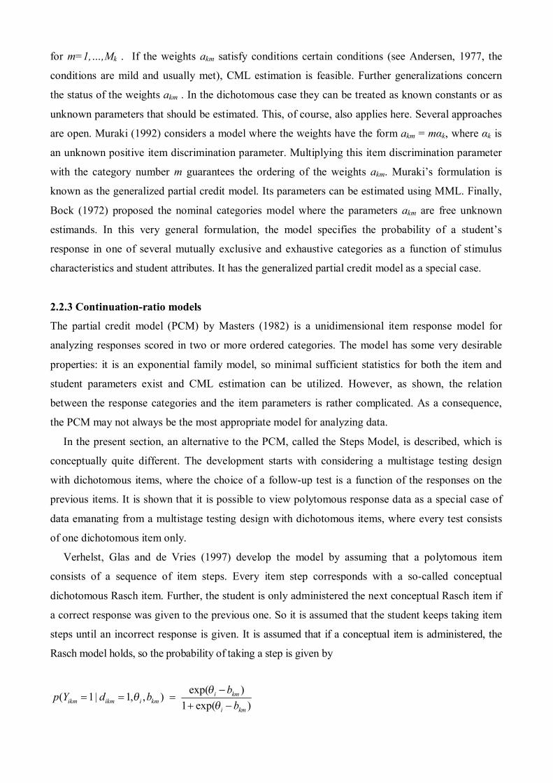
as the parameter of category m alone. Masters (1982) shows that these conditional probabilities can

be rewritten to the unconditional probability of a student i scoring in category m on item k given by

g=1

1 g=1

exp( )( 1| , )

1 expk

m

i km

ikm i k M h

i kgh

m bp Y b

h b

θθ

θ=

−= =

+ −

∑

∑ ∑ (13)

for m=1,…,Mk . This model is known as the partial credit model (PCM). The important part in this

formula is the nominator; the denominator is a sum over all nominators and it assures the response

probabilities sum to one. Note that the probability of a response in the zero-category, denoted Yik0 =

1, has a nominator 1 and a denominator as in Formula (13).

The PCM can also be derived from a different perspective. As mentioned above, Fischer (1974)

has shown that the Rasch model for dichotomous items can be derived from a set of assumptions,

including sufficiency of the number correct score. In the PCM, the sufficient statistic for the ability

parameter is the weighted sum score

1 1

kMk

i ik ikmk m

R d mY= =

= ∑ ∑

that is, the sum of the weights m of the categories in which the items were responded to (Andersen,

1977). However, this immediately suggests a generalization of the model. Authors as Kelderman

(1984, 1989), Verhelst and Glas (1995) and Wilson and Masters (1993) have considered various

more general sufficient statistics for ability. Among other models, they all consider the weighted-

score statistic

1 1

kMk

i ik km ikmk m

R d a Y= =

= ∑ ∑

where the weights are positive, integer-valued and ordered ak1<ak2<,…,<akMk. This results in a

model

g=1

1 g=1

exp( )( 1| , , ) ,

1 expk

m

km i km

ikm i k k M h

kh i kgh

a bp Y a b

a b

θθ

θ=

−= =

+ −

∑

∑ ∑ (14)

for m=1,…,Mk . If the weights akm satisfy conditions certain conditions (see Andersen, 1977, the

conditions are mild and usually met), CML estimation is feasible. Further generalizations concern

the status of the weights akm . In the dichotomous case they can be treated as known constants or as

unknown parameters that should be estimated. This, of course, also applies here. Several approaches

are open. Muraki (1992) considers a model where the weights have the form akm = mαk, where αk is

an unknown positive item discrimination parameter. Multiplying this item discrimination parameter

with the category number m guarantees the ordering of the weights akm. Muraki’s formulation is

known as the generalized partial credit model. Its parameters can be estimated using MML. Finally,

Bock (1972) proposed the nominal categories model where the parameters akm are free unknown

estimands. In this very general formulation, the model specifies the probability of a student’s

response in one of several mutually exclusive and exhaustive categories as a function of stimulus

characteristics and student attributes. It has the generalized partial credit model as a special case.

2.2.3 Continuation-ratio models

The partial credit model (PCM) by Masters (1982) is a unidimensional item response model for

analyzing responses scored in two or more ordered categories. The model has some very desirable

properties: it is an exponential family model, so minimal sufficient statistics for both the item and

student parameters exist and CML estimation can be utilized. However, as shown, the relation

between the response categories and the item parameters is rather complicated. As a consequence,

the PCM may not always be the most appropriate model for analyzing data.

In the present section, an alternative to the PCM, called the Steps Model, is described, which is

conceptually quite different. The development starts with considering a multistage testing design

with dichotomous items, where the choice of a follow-up test is a function of the responses on the

previous items. It is shown that it is possible to view polytomous response data as a special case of

data emanating from a multistage testing design with dichotomous items, where every test consists

of one dichotomous item only.

Verhelst, Glas and de Vries (1997) develop the model by assuming that a polytomous item

consists of a sequence of item steps. Every item step corresponds with a so-called conceptual

dichotomous Rasch item. Further, the student is only administered the next conceptual Rasch item if

a correct response was given to the previous one. So it is assumed that the student keeps taking item

steps until an incorrect response is given. It is assumed that if a conceptual item is administered, the

Rasch model holds, so the probability of taking a step is given by

exp( )( 1| 1, , ) 1 exp( )

i kmikm ikm i km

i km

bp Y d bb

θθ

θ−

= = =+ −

where dkm is a design variable as defined for dichotomous items by Formula (3), bkm is the difficulty

parameters of step m within item k. Let rik be the number of item steps taken within item k, that is,

kMkmm=1k kmr yd= ∑

In Table 2.12, for some item with Mk = 3, all possible responses yk , yk = (yk1,yk2,yk3) are enumerated,

together with the associated probabilities ( | , )k kP y bθ .

Table2.12 Response Probabilities in the Continuation-Ratio Model.

yk rk ( | , )k kP y bθ

0,c,c

0 1

1 1 exp( )i kbθ+ −

1,0,c

1 [ ][ ]1

1 2

exp( ) 1 exp( ) 1 exp( )

i k

i k i k

bb b

θθ θ

−+ − + −

1,1,0

2 [ ][ ][ ]1 2

1 2 3

exp( ) exp( ) 1 exp( ) 1 exp( ) 1 exp( )

i k i k

i k i k i k

b bb b b

θ θθ θ θ

− −+ − + − + −

1,1,1

3 [ ][ ][ ]1 2 2

1 2 3

exp( ) exp( )exp( ) 1 exp( ) 1 exp( ) 1 exp( )

i k i k i k

i k i k i k

b b bb b b

θ θ θθ θ θ

− − −+ − + − + −

From inspection of Table 2.12, it can be easily verified that in general

[ ]1

min( , 1)

1

exp( | , )

1 exp(

k

k k

M

k kmm

k k M r

kmh

r bP y b

b

θθ

θ

=+

=

−

+ −

∑

∏ (15)

where min(Mk,rk+1) stands for the minimum of Mk and rk+1. The model does not have sufficient

statistics, so it cannot be estimated using CML (Glas, 1988b). The model is straightforwardly

generalized to a model where the item steps are modeled by a 2PLM, or to a normal ogive formulation.

With the definition of a normal ability distribution, any program for dichotomous data that can compute

MML estimates in the presence of missing data can estimate the parameters. The same holds in a

Bayesian framework, where any software package that can perform MCMC estimation with incomplete

data can be used to estimate the model parameters.

2.2.4 Cumulative probability models

In adjacent-category models are generally based on a definition of the probability that the score, say

Rk, is equal to m conditional on the event that it is either m or m-1, for instance,

( | or 1) ( ( ))k k k k kmP R m R m R m a bθ= = = − = Ψ −

Continuation-ratio models, on the other hand, are based on a definition of the probability of scoring

equal to, or higher than m given that the score is at least m-1, that is

( | 1) ( ( ))k k k kmP R m R m a bθ≥ ≥ − = Ψ −

An alternative, yet older, approach can be found in the model proposed by Samejima (1969). Here

the probability of scoring equal to, or higher than m is not considered conditional on the event that

the score is at least m-1, but this probability is defined by

( ) ( ( ))k k kmP R m a bθ≥ = Ψ −

It follows that the probability of scoring in a response category m is given by

( 1)( ) ( 1| , ) ( ( )) ( ( ))k ikm k k km k k mP R m P Y b a b a bθ θ θ += = = = Ψ − − Ψ − (16)

for m=1,…Mk-1. Since the probability of obtaining a score Mk + 1 is zero and since everyone can at

least obtain a score 0, it is reasonable to set ( 1) 0k kP R M≥ + = and ( 0) 1kP R ≥ = . As a result

0 1( 0) ( 1| , ) 1 ( ( ))k ik k k kP R P Y b a bθ θ= = = = − Ψ −

and

( ) ( 1| , ) ( ( ))k kk k ikM k k kMP R M P Y b a bθ θ= = = = Ψ −

To assure that the differences in Formula (16) are positive, it must hold that

( 1)( ( )) ( ( ))k km k k ma b a bθ θ +Ψ − > Ψ − , which implies that b1<b2<,…,<bMk. Further, contrary to the case

of continuation-ratio models, the discrimination parameter ak must be the same for all item steps.

The model can both be estimated in a likelihood-based and Bayesian framework. The former is

done using MML estimation; the procedure is implemented in the program Multilog (Thissen, 1991).

Johnson and Albert (1999) worked out the latter approach in detail.

2.3 Multidimensional Models

In many instances, it suffices to assume that ability is unidimensional. However, in other instances, it

may be a priori clear that multiple abilities are involved in producing the manifest responses, or the

dimensionality of the ability structure might not be clear at all. In such cases, multidimensional IRT

(MIRT) models can serve confirmatory and explorative purposes, respectively. As this terminology

suggests, many MIRT models are closely related to factor analytic models; in fact, Takane and de

Leeuw (1987) have identified a class of MIRT models that is equivalent to a factor analysis model

for categorical data.

MIRT models for dichotomously scored items were first presented by McDonald (1967) and Lord

and Novick (1968). These authors use a normal ogive to describe the probability of a correct

response. The idea of this approach is that the dichotomous response of student i to item k is

determined by an unobservable continuous random variable. This random variable has a standard

normal distribution and the probability of a correct response is equal to the probability mass below

some cut-off point ikη . That is, the probability of a correct response is given by

1( ) ( ) ( )

Q

k i ik kq iq kq

p a bθ η θ=

= Φ = Φ −∑ (17)

where (.)Φ is the cumulative standard normal distribution, iθ is a vector with elements ,iqθ 1,...,q Q= ,

which are the Q ability parameters (or factor scores) of student i, bk is the difficulty of item k, and akq

( 1,...,q Q= ) are Q factor loadings expressing the relative importance of the Q ability dimensions for

giving a correct response to item j. For the unidimensional IRT models discussed above, the

probability of a correct response as function of ability could be represented by a so-called item

response curve. For MIRT models, however, the probability of a correct response depends on a Q-

dimensional vector of ability parameters θi so Pk(θi) is now a surface rather than a curve. An

example of an item response surface by Reckase (1977) is given in Figure 2.6.

The item pertains to two ability dimensions. The respondents’ ability vectors (θi1, θi2) represent

points in the ability space and for every point the probability of a correct response is given by the

matching point on the surface. Note that if one dimension is held constant, the probability of a

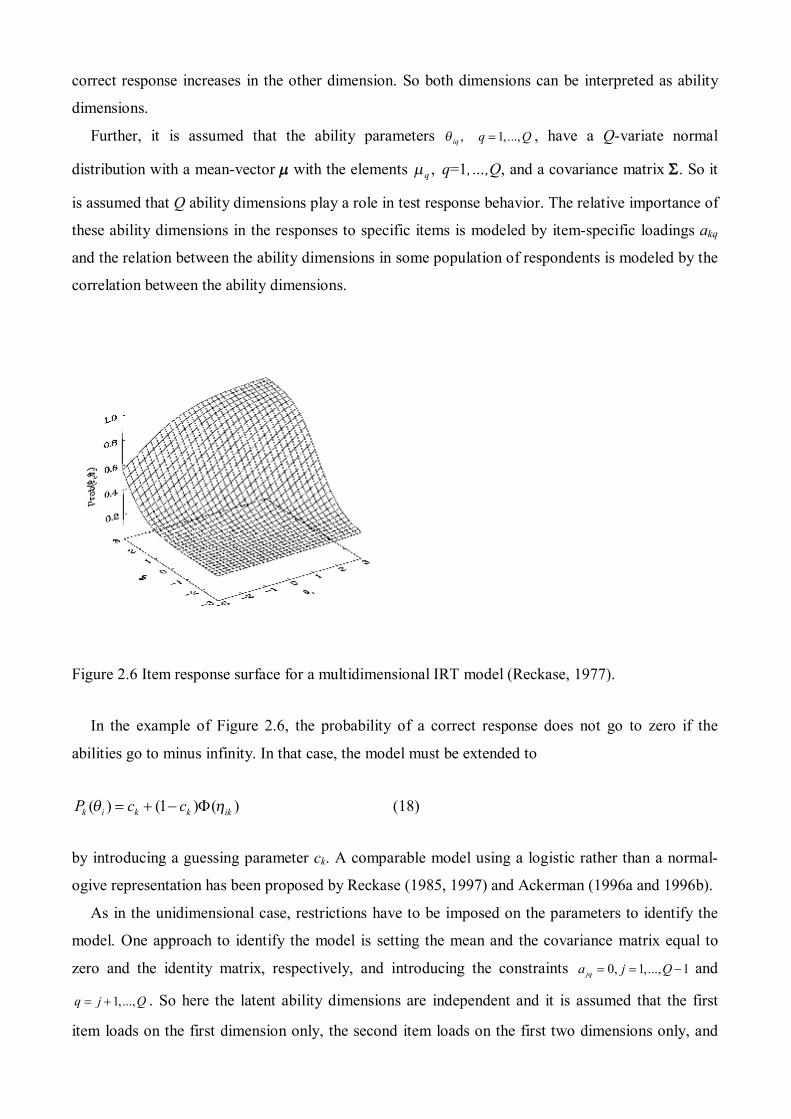
correct response increases in the other dimension. So both dimensions can be interpreted as ability

dimensions.

Further, it is assumed that the ability parameters ,iqθ 1,...,q Q= , have a Q-variate normal

distribution with a mean-vector µ with the elements ,qµ q=1,…,Q, and a covariance matrix Σ. So it

is assumed that Q ability dimensions play a role in test response behavior. The relative importance of

these ability dimensions in the responses to specific items is modeled by item-specific loadings akq

and the relation between the ability dimensions in some population of respondents is modeled by the

correlation between the ability dimensions.

Figure 2.6 Item response surface for a multidimensional IRT model (Reckase, 1977).

In the example of Figure 2.6, the probability of a correct response does not go to zero if the

abilities go to minus infinity. In that case, the model must be extended to

( ) (1 ) ( )k i k k ikP c cθ η= + − Φ (18)

by introducing a guessing parameter ck. A comparable model using a logistic rather than a normal-

ogive representation has been proposed by Reckase (1985, 1997) and Ackerman (1996a and 1996b).

As in the unidimensional case, restrictions have to be imposed on the parameters to identify the

model. One approach to identify the model is setting the mean and the covariance matrix equal to

zero and the identity matrix, respectively, and introducing the constraints 0, 1,..., 1 jqa j Q= = − and

1,...,q j Q= + . So here the latent ability dimensions are independent and it is assumed that the first

item loads on the first dimension only, the second item loads on the first two dimensions only, and

so on, until item 1 Q − , which loads on the first 1 Q − dimensions. All other items load on all

dimensions. An alternative approach to identifying the model is setting the mean equal to the zero,

considering the covariance parameters of proficiency distribution as unknown estimands. The model

is then further identified by imposing the restrictions, 1, if , jq j qα = = and 0, jqα = if , j q≠ for

1,..., j Q= and 1,...,q Q= . So here the first item defines the first dimension, the second item defines the

second dimension, and so forth, until item Q which defines the Q-th dimension. Further, the

covariance matrix Σ describes the relation between the thus defined latent dimensions.

In general however, these identification restrictions will be of little help to provide an

interpretation of the ability dimensions. Therefore, as in an exploratory factor analysis, the factor

solution is usually visually or analytically rotated. Often, the rotation scheme is devised to

approximate Thurstone's simple-structure criterion (Thurstone, 1947), where the factor loadings are

split into two groups, the elements of the one tending to zero and the elements of the other toward

unity.

As an alternative, several authors (Glas, 1992; Adams & Wilson, 1996; Adams, Wilson & Wang,

1997; Béguin & Glas, 2001) suggest to identify the dimensions with subscales of items loading on

one dimension only. The idea is to either identify these S < Q subscales a priori in an confirmatory

mode, or to identify them using an iterative search. The search starts with fitting a unidimensional

IRT model by discarding non-fitting items. Then, in the set of discarded items, items that form a

second unidimensional IRT scale are identified, and this process is repeated until S subscales are

formed. Finally, the covariance matrix Σ between the latent dimensions is estimated either by

imputing the item parameters found in the search for subscales, or concurrently with the item

parameters leaving the subscales intact.

For the generalization of the MIRT model to polytomous items, the same three approaches are

possible as in the unidimensional case: adjacent-category models, continuation-ratio models and

cumulative probability models. All three possibilities are feasible, but only the former and the latter

will be discussed here to explicate some salient points.

In the framework of the cumulative probabilities approach, a model for polytomous items with Mk

ordered response categories can be obtained by assuming Mk standard normal random variables, and

Mk cut-off points ikmη for m = 1,…,Mk. The probability that the response is in category m is given by

( 1)( ) ( ) ( )km i ik m ikmp θ η η−= Φ − Φ

where 1

,Q

ikm kq iq kmq

bη α θ=

= −∑ ( 1) ,ik m ikmη η− > 0 ,ikη = ∞ and kikMη = −∞

Takane and de Leeuw (1987) point out that also this model is both equivalent to a MIRT model for

graded scores (Samejima, 1969) and a factor analysis model for ordered categorical data (Muthén,

1984).

In the framework of adjacent categories models, the logistic versions of the probability of a

response in category m can be written as

1 1( ) exp / ( , , )

Q m

km i kq iq kh i k kq h

p m a b h a bθ θ θ= =

= −

∑ ∑ (19)

where ( , , )i k kh a eθ is some normalizing factor that assures the sum over all possible responses on an

item is equal to one. The probability ( )km ip θ is determined by the compound 1

Q

kq iqq

a θ=

∑ so every item

addresses the abilities of a respondent in a unique way. Given this ability compound, the

probabilities of responding a certain category are analogous to the unidimensional partial credit

model by Masters (1982). Firstly, the factor m indicates that the response categories are ordered and

that the expected item score increases as the ability compound 1

Q

kq iqq

a θ=

∑ increases. And secondly, the

item parameters bkh are the points where the ability compound has such a value that the odds of

scoring either in category m-1 or m are equal.

3. Data collection designs

In the introduction of the previous chapter, it was shown that one of the important features of IRT is

the possibility of analyzing so-called incomplete designs. In incomplete designs the administration of

items to persons is such, that different groups of persons have responded to different sets of items. In the

present section, a number of possible data collection designs will be discussed.

A design can be represented in the form of a persons-by-items matrix. As an example, consider the

design represented in Figure 3.1. This figure is a graphical representation of a design matrix with as

entries the item administration variables dik (I = 1,…,N and k = 1,…,K) defined by Formula (3) in the

previous chapter. The item administration variable dik was equal to 1 if person i responded to item k,

and 0 otherwise. At this moment, it is not yet specified what caused the missing data. There may be

no response because the item was not presented, or because the item was skipped, or because the

item was not reached. In the sequel it will be discussed under which circumstances the design will

interfere with the inferences. For the time being assume that the design was fixed by the test

administrator and that the design does not depend on an a-priori estimate of the ability level of the

respondents.

Figure 3.1 Design linked by common items.

In the example, the total number of items is K = 25. The design consists of two groups of students,

the first group responded to the items 1 to 15, and the second group responded to items 11 to 25. In

general, assume that B different subsets of the total of K items have been administered, each to an

exclusive subset of the total sample of respondents. These subsets of items will be indicated by the term

'booklets'. Let I be the set of the indices of the items, so I = {1,…,K}. Then the booklets are formally

defined as non-empty subsets of Ib of I, for b = 1,…,B. Let Kb denote the number of elements of Ib , that

is, Kb is the number of items in booklet b. Next, let V denote the set of the indices of the respondents, so

V = {1,…,N}, where N is the total number of respondents in the sample. The sub-sample of respondents

getting booklet b is denoted by Vb and the number of respondents administered booklet b is denoted Nb.

The subsets Vb are mutually exclusive, so N = Σb Nb.

To obtain parameters estimates on a common scale, the design has to be linked. For instance, the

design of Figure 3.1 is linked because the two booklets are linked by the items 11 to 15, which are

common to both booklets. A formal definition of a linked design entails that for any two booklets a and

b in the design, there must exist a sequence of booklets with item index sets Ia, Ib1, Ib2…, Ib such that

any two adjacent booklets in the sequence have common items or are administered to samples from the

same ability distribution. The sequence may just consist of Ia and Ib . Assumptions with respect to

ability distributions do not play a part in CML estimation. So CML estimation is only possible if the

design is linked by sequence Ia, Ib1, Ib2…, Ib where adjacent booklets have common items.

Figure 3.2 Linking by common persons.

This definition may lead to some confusion because it interferes with the more commonly used terms

“linking by common items” and “linking by common persons”. Figure 3.1 gives an example of a design

linked by common items because the two booklets have common items. Figure 3.2 gives an example of

a design that is commonly labeled “linked by common persons”. The definition of a linked design

applies here because the first and second booklet have common items and the second and last booklet

have common items. Further, the first and last booklet are linked via the second booklet.

An example of linking via common ability distributions is given in Figure 3.3. Again, common

items link the middle two booklets. The respondents of the first two booklets are assumed to be

drawn from the first ability distribution and the respondents of the last two booklets are assumed to

be drawn from a second ability distribution. It must be emphasized that, in general, designs linked by

common items are far preferable to designs that are only linked by common distributions, since the

assumptions concerning these distributions add to the danger that the model as a whole does not fit the

data. Assumptions on ability distributions should be used to support answering specific research

questions, not as a ploy for mending poor data collection strategies.

Figure 3.3 Linking by a common distribution.

4. Scope of the program as released

The present release pertains to a version which can be used to run analyses with PISA data. The

program focuses on MML estimation of the PCM, but the GPCM and a multidimensional version of

the GPCM is also supported. The model for the probability of a student i scoring in category m on

item k given by

q=1

1 q=1

exp( 1)

1 expk

Q

k kq iq km

ikm M Q

k kq iq khh

w a tp Y

w a t

θ

θ=

−

= =

+ −

∑

∑ ∑ (20)

for m=1,…,Mk . Here, wk is a fixed item scoring weight, which is usually equal to one. An exception

is the OPLM where the weights are explicitly chosen as positive integers. The program allows for

weights between 1 and 8. The item parameters tkm are often transformed into so-called item-

category bounds parameters using the transformation

g=1

m

km kgt b= ∑ .

The unidimensional version of the model can then be written as

( )

( )g=1

1 g=1

exp( 1| , )

1 expk

m

k k i kg

ikm i k M h

k k i kgh

w a bp Y b

w a b

θθ

θ=

−

= =

+ −

∑

∑ ∑ (21)

5. The structure of the data file

The program MIRT is suited for analyzing incomplete designs and handling missing data. The data

can be organized in two ways. We will start with the recommended one. As an example consider

Figure 5.1. Suppose that there are K = 10 items in the design and 2 booklets. The first booklet

contains the items 1-5 and 7-8. So the students administered this booklet responded to 7 items. The

second booklet contained the items 1-2, 6, 9-10. So the students administered this booklet responded

to 5 items. Every record in the data file pertains to a student. Note that there are 10 students. The

columns 1-2 contain the booklet number. Note that there are 2 booklets. Further, the columns 3-5

contain an optional student ID. The student IDs must be integer valued. They are echoed on files

containing the student’s ability scores. The columns 7-13 contain the item responses. In the example,

the responses are scored between 0 and 3. A 9 stands for a missing response. Only the responses to

items figuring in a booklet are entered into the data file. For the first booklet, the program is

informed that the columns 7-11 pertain to the items 1-5, and the columns 12-13 pertain to the items

7-8. In the same manner, for the second booklet, the columns 7-11 pertain to the items 1, 2, 6, 9 and

10, in that order.

1 2 3 4 5 6 7 8 9 10 11 12 13

1 1 1 0 2 1 3 0 9

1 2 0 0 2 1 0 0 0

1 3 0 1 0 3 2 1 0

1 4 0 0 9 1 3 3 3

1 5 1 0 0 0 2 0 2

2 6 2 0 0 0 0

2 7 1 1 1 9 3

2 8 3 3 3 3 3

2 9 2 1 2 1 2

2 1 0 0 0 0 0 0

Figure 5.1

Recommended format of a data file

An alternative way of organizing the data file is depicted in Figure 5.2. The person and booklet IDs

are in the same positions. However, the program is now told that both booklets consisted of the same

10 items and the design is handled by entering the missing data code 9 for the items not responded

to. The reason for recommending the first format is efficiency of computer storage. The

computational procedures are generally not affected.

1 2 3 4 5 6 7 8 9 10 11 12 13 14 15 16

1 1 1 0 2 1 3 9 0 9 9 9

1 2 0 0 2 1 0 9 0 0 9 9

1 3 0 1 0 3 2 9 1 0 9 9

1 4 0 0 9 1 3 9 3 3 9 9

1 5 1 0 0 0 2 9 0 2 9 9

2 6 2 0 9 9 9 0 9 9 0 0

2 7 1 1 9 9 9 1 9 9 9 3

2 8 3 3 9 9 9 3 9 9 3 3

2 9 2 1 9 9 9 2 9 9 1 2

2 1 0 0 0 9 9 9 0 9 9 0 0

Figure 5.2

Alternative format of a data file

The following points should be kept in mind:

• The booklet number has the same position in all records. It is a positive integer. However, the

booklet numbers need not be consecutive. A booklet number is always required, even if there

is only one booklet. The records pertaining to a specific booklet need not be consecutively

grouped together.

• In every record, the booklet number, the (optional) person ID and the data should start in the

same column.

• The item responses are integers. They are unweighed item scores.

• Blanks in the data file are interpreted as zeros.

• The missing data code is always 9.

6. Running the program

6.1. Introduction

The program consists of six packages

Programs Functionality remark

MIRT.EXE Shell

MIRT1.EXE Main MML estimation program

MIRT0.EXE CML and MML estimation

program Rasch model

Not supplied here

MIRT2.EXE CML and MML estimation

program OPLM

Not supplied here

MIRT3.EXE MML estimation program linear

models on item and/or person

parameters

Not supplied here

MIRT4.EXE MCMC estimation program Not supplied here

Just copy the packages to a dedicated directory, for instance, D:\MIRT or C:\MIRT_PROGRAM.

The path, say C:\MIRT_PROGRAM\MIRT.EXE, should not contain blanks! So do not put the

software on your desk-top. This will also hold for the run files and output files created by the

program.

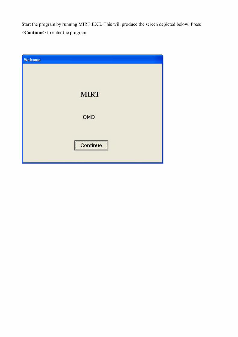
Start the program by running MIRT.EXE. This will produce the screen depicted below. Press

<Continue> to enter the program

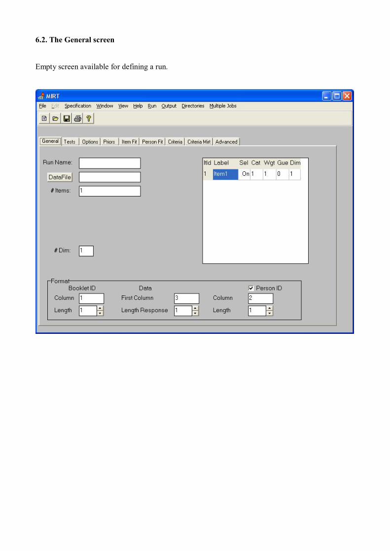
6.2. The General screen

Empty screen available for defining a run.

However, existing runs can also be entered and edited. Choose the <File> option, at the left-hand

side in the top row and then select <Open>. The produces a list of available runs. The runs are

stored in files named JOBNAME.SPC. In the present example, we choose

HOMPOS_COMP_DEU.SPC.

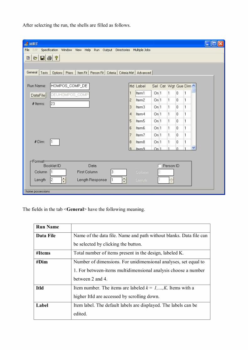
After selecting the run, the shells are filled as follows.

The fields in the tab <General> have the following meaning.

Run Name

Data File Name of the data file. Name and path without blanks. Data file can

be selected by clicking the button.

#Items Total number of items present in the design, labeled K.

#Dim Number of dimensions. For unidimensional analyses, set equal to

1. For between-items multidimensional analysis choose a number

between 2 and 4.

Itld Item number. The items are labeled k = 1,…,K. Items with a

higher ItId are accessed by scrolling down.

Label Item label. The default labels are displayed. The labels can be

edited.

Sel By toggling <On/Off>, items can be selected or ignored in an

analysis. Deselecting an item overrides selections within booklets

defined in the Tests tab.

Cat Number of response categories minus the zero category. The item

responses are coded m=0,…,Mk. Note that M. is the number to be

entered here. So for dichotomous items, Mk=1.

Wgt Item scoring weight. An integer between 1 and 8. This weight is

defined in the general model as displayed in (20) and (21) as wk.

Gue A toggle <0/1> to add a guessing parameter to an item to impose

the 3PLM for that item.

Dim Dimension on which the item loads.

BookletID Position and length of the Booklet ID in a record.

Data Position of the first item response and the number of positions for

each item response

Person ID If flagged, the position and length of the person ID. This person ID

is echoed in files with person parameter estimates. The person ID

is restricted to be an integer number.

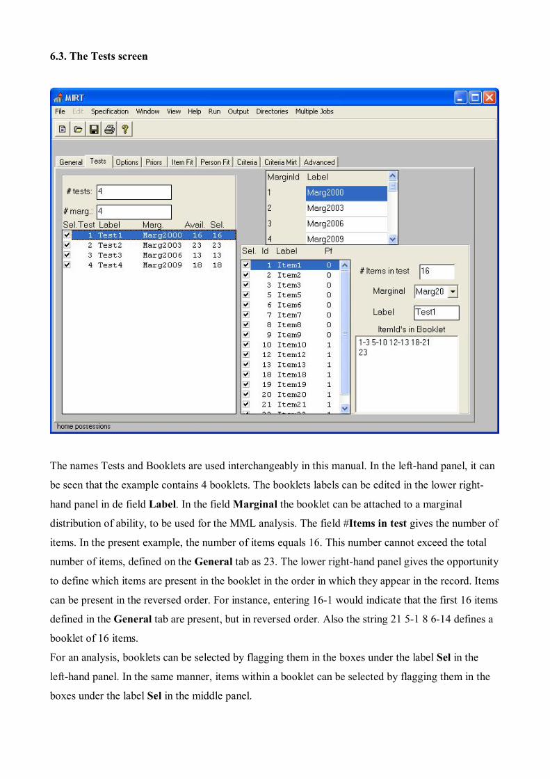
6.3. The Tests screen

The names Tests and Booklets are used interchangeably in this manual. In the left-hand panel, it can

be seen that the example contains 4 booklets. The booklets labels can be edited in the lower right-

hand panel in de field Label. In the field Marginal the booklet can be attached to a marginal

distribution of ability, to be used for the MML analysis. The field #Items in test gives the number of

items. In the present example, the number of items equals 16. This number cannot exceed the total

number of items, defined on the General tab as 23. The lower right-hand panel gives the opportunity

to define which items are present in the booklet in the order in which they appear in the record. Items

can be present in the reversed order. For instance, entering 16-1 would indicate that the first 16 items

defined in the General tab are present, but in reversed order. Also the string 21 5-1 8 6-14 defines a

booklet of 16 items.

For an analysis, booklets can be selected by flagging them in the boxes under the label Sel in the

left-hand panel. In the same manner, items within a booklet can be selected by flagging them in the

boxes under the label Sel in the middle panel.

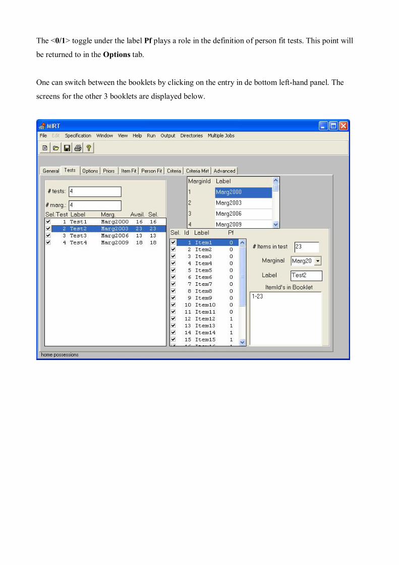
The <0/1> toggle under the label Pf plays a role in the definition of person fit tests. This point will

be returned to in the Options tab.

One can switch between the booklets by clicking on the entry in de bottom left-hand panel. The

screens for the other 3 booklets are displayed below.

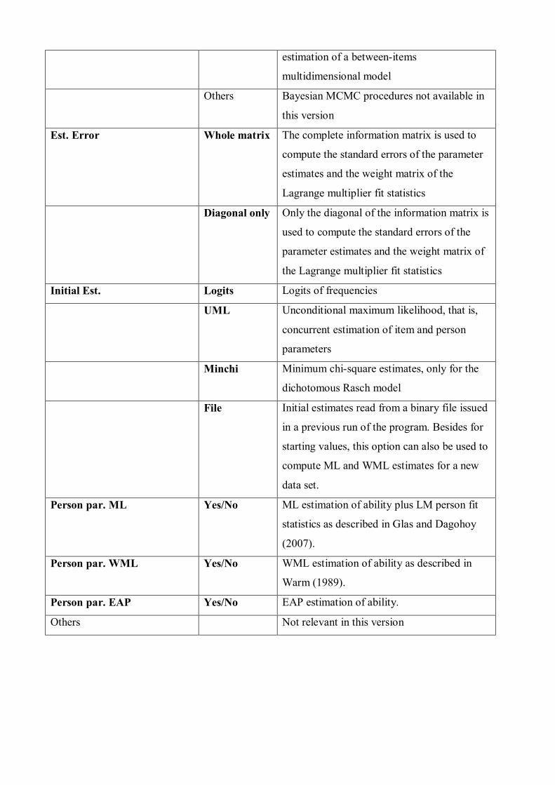
6.4. The Options screen

Field Options Remarks

Title Title displayed on output

Model PCM PCM, 1PLM in case of dichotomous items

GPCM GPCM, 2PLM in case of dichotomous items,

3PLM if items with guessing parameter

specified in General screen

Others Not relevant here

Estimation MML MML estimation, starting with 1PLM/PCM

and continuing with 2PLM/3PLM/GPCM if

requested so in previous field

MulMML Additional to the procedure above, and

estimation of a between-items

multidimensional model

Others Bayesian MCMC procedures not available in

this version

Est. Error Whole matrix The complete information matrix is used to

compute the standard errors of the parameter

estimates and the weight matrix of the

Lagrange multiplier fit statistics

Diagonal only Only the diagonal of the information matrix is

used to compute the standard errors of the

parameter estimates and the weight matrix of

the Lagrange multiplier fit statistics

Initial Est. Logits Logits of frequencies

UML Unconditional maximum likelihood, that is,

concurrent estimation of item and person

parameters

Minchi Minimum chi-square estimates, only for the

dichotomous Rasch model

File Initial estimates read from a binary file issued

in a previous run of the program. Besides for

starting values, this option can also be used to

compute ML and WML estimates for a new

data set.

Person par. ML Yes/No ML estimation of ability plus LM person fit

statistics as described in Glas and Dagohoy

(2007).

Person par. WML Yes/No WML estimation of ability as described in

Warm (1989).

Person par. EAP Yes/No EAP estimation of ability.

Others Not relevant in this version

6.5. The priors screen

MIRT supports the use of priors for the item parameters. They are introduced using a toggle

<Yes/No>. The prior for the a-parameter is log-normal, the prior for the b-parameter is normal and

the prior for the c-parameter is a Beta-distribution.

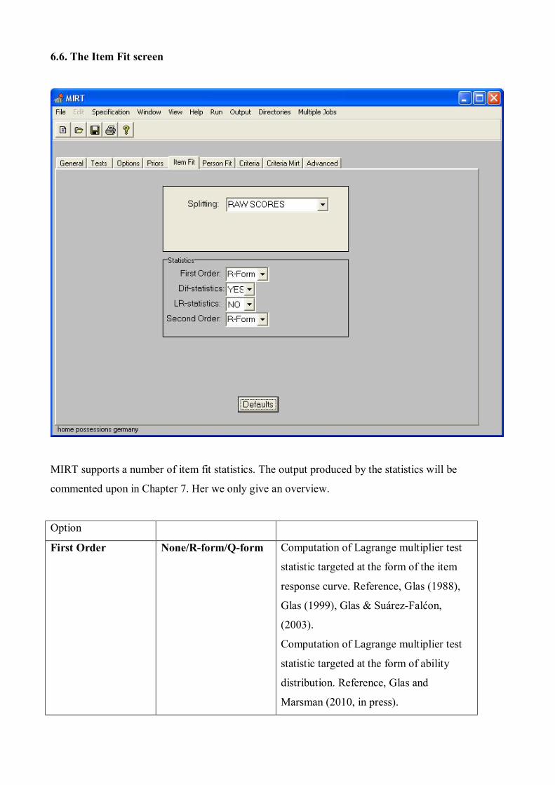
6.6. The Item Fit screen

MIRT supports a number of item fit statistics. The output produced by the statistics will be

commented upon in Chapter 7. Her we only give an overview.

Option

First Order None/R-form/Q-form Computation of Lagrange multiplier test

statistic targeted at the form of the item

response curve. Reference, Glas (1988),

Glas (1999), Glas & Suárez-Falćon,

(2003).

Computation of Lagrange multiplier test

statistic targeted at the form of ability

distribution. Reference, Glas and

Marsman (2010, in press).

Dif-statistics Yes/No Computation of Lagrange multiplier test

statistic targeted at differential item

functioning across booklets. Reference,

Glas (1998).

LR-statistics Yes/No Andersen’s likelihood ratio test statistic,

Rasch model only. Reference: Andersen

(1977)

Second Order None/R-form/Q-form Computation of Lagrange multiplier test

statistic targeted at local independence.

Reference, Glas (1988), Glas (1999), Glas

& Suárez-Falćon, (2003).

Splitting Raw Scores First order statistics based on subgroups

formed using their raw scores

External Variable First order statistics based on subgroups

formed using an external variable

6.8. The Person Fit screen

Not relevant here. Person fit statistics are computed upon choosing ML-estimation in the Options

screen.

6.9. The Criteria screen

Not relevant here.

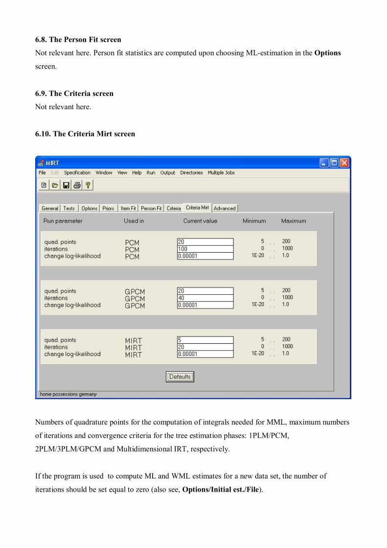
6.10. The Criteria Mirt screen

Numbers of quadrature points for the computation of integrals needed for MML, maximum numbers

of iterations and convergence criteria for the tree estimation phases: 1PLM/PCM,

2PLM/3PLM/GPCM and Multidimensional IRT, respectively.

If the program is used to compute ML and WML estimates for a new data set, the number of

iterations should be set equal to zero (also see, Options/Initial est./File).

6.11. The Advanced screen

This screen is used to select item pairs for the computation of item pairs for the test of local

independence. Shown are the default pairs, which are pairs of consecutive items.

6.12. Starting the Computations and viewing the output

It is recommended to save a setup before running the computational module via File/Save as or via

the save-button.

Then choose RUN and choose the middle of the three displayed options, which is MIRT (the

options RSP and EIRT are currently blocked). This results in the following display where the

option Yes must be selected.

The main output is written to a file JOBNAME.MIR. The file can be viewed by choosing the

Output option in the top row followed by the option View. The output is written to a text file which

can be accessed using most general purpose editors, such as Notepad or Word.

Information on person parameters is written to

JOBNAME.WRM1 WML estimation of ability 1PLM/PCM.

JOBNAME.WRM2 WML estimation of ability 2PLM/GPCM

JOBNAME.PRS1 ML estimation of ability plus LM person fit statistics

1PLM/PCM

JOBNAME.PRS2 ML estimation of ability plus LM person fit statistics

2PLM/GPCM

JOBNAME.EAP1 EAP estimation of ability. 1PLM/PCM

JOBNAME.EAP2 EAP estimation of ability. 2PLM/GPCM

JOBNAME.EAP3 Multidimensional EAP estimation of ability.

Finally, the program creates a whole range of additional fils which are of no importance now. The

only exception is JOBNAME.BIN1 and JOBNAME.BIN2, which are binary files with the item

parameters for the 1PLM/PCM and 2PLM/3PLM/GPCM, respectively.

7. The Output

7.1. The file JOPBNAME.MIR

First page echoes run information

******************************************************************************** * * * MIRT 7- 8-2010 15:46: 9 * * * ******************************************************************************** MIRT Scaling Program Version 1.01 March 1, 2010 RUN TITLE: home possessions germany RUN NAME: HOMPOS_COMP_DEU RUN SPECIFICATION: NUMBER OF ITEMS IN DESIGN : 23 NUMBER OF TESTS IN DESIGN : 4 NUMBER OF MARGINALS IN DESIGN : 4 NUMBER OF DIMENSIONS : 1 ESTIMATION PROCEDURE : MML 3PL / PCM CONFIDENCE INTERVALS COMPUTED USING COMPLETE INFORMATION MATRIX STARTING VALUES: LOGITS MODEL FIT EVALUATED USING: R2-STATISTIC ML ESTIMATES OF ABILITY COMPUTED WML ESTIMATES OF ABILITY COMPUTED EAP ESTIMATES OF ABILITY COMPUTED PRIOR SPECS A B C : 0 0 0 0.00 0.50 0.50 5.00 5.00 17.00 NUMBER OF QUADRATURE POINTS: 20 20 5 NUMBER OF ITERATIONS : 100 40 20 STOP-CRITERIA : 0.1000E-04 0.1000E-04 0.1000E-04 INPUT FILE: D:\mirt-win8\DEUHOMPOS_COMPLETE.DAT DATA READ USING FORMAT: (T1,I2,T3,23I1) NUMBER OF ITEMS IN INPUT FILE 23 NUMBER OF ITEMS SELECTED FOR ANALYSIS 23 NUMBER OF PERSONS SELECTED FOR ANALYSIS 10000 ================================================================================

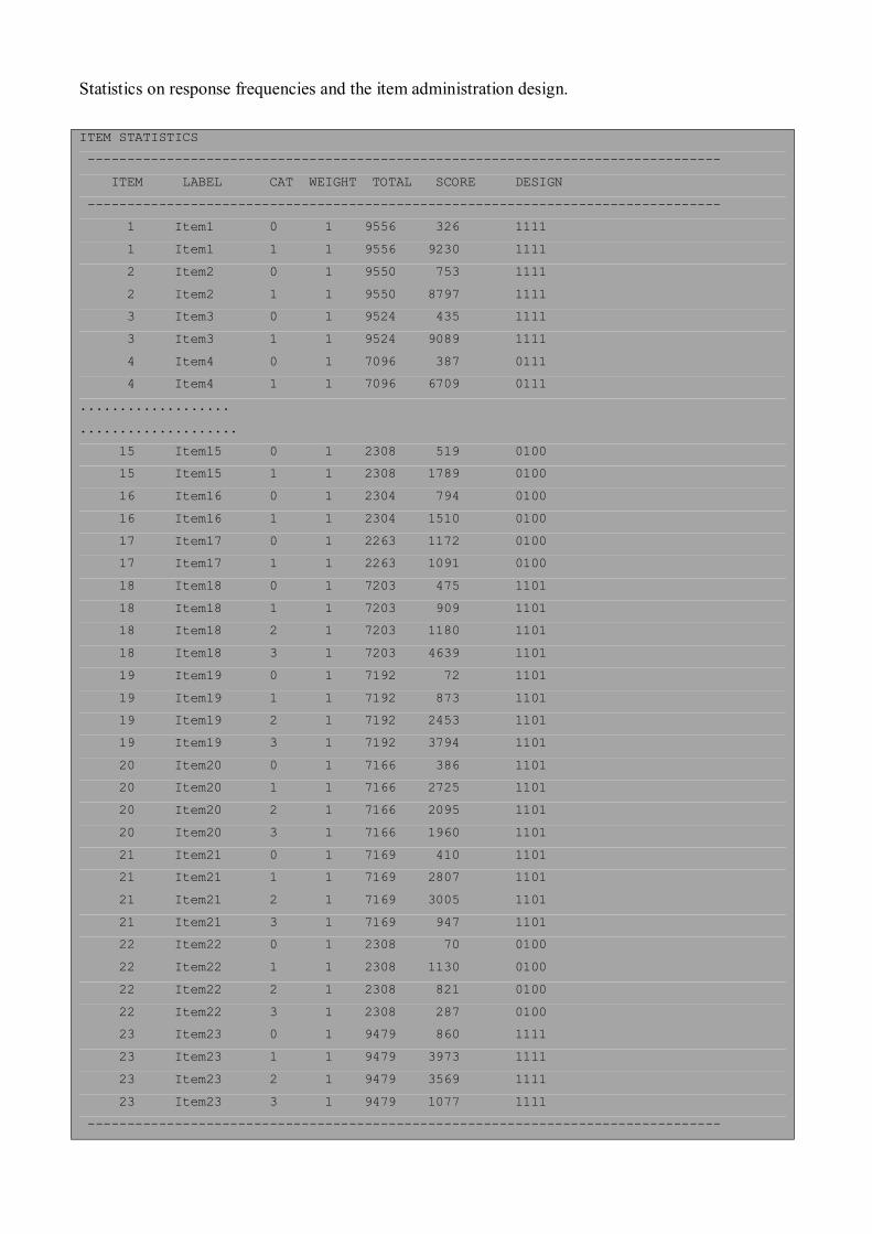
Statistics on response frequencies and the item administration design.

ITEM STATISTICS -------------------------------------------------------------------------------- ITEM LABEL CAT WEIGHT TOTAL SCORE DESIGN -------------------------------------------------------------------------------- 1 Item1 0 1 9556 326 1111 1 Item1 1 1 9556 9230 1111 2 Item2 0 1 9550 753 1111 2 Item2 1 1 9550 8797 1111 3 Item3 0 1 9524 435 1111 3 Item3 1 1 9524 9089 1111 4 Item4 0 1 7096 387 0111 4 Item4 1 1 7096 6709 0111 ................... .................... 15 Item15 0 1 2308 519 0100 15 Item15 1 1 2308 1789 0100 16 Item16 0 1 2304 794 0100 16 Item16 1 1 2304 1510 0100 17 Item17 0 1 2263 1172 0100 17 Item17 1 1 2263 1091 0100 18 Item18 0 1 7203 475 1101 18 Item18 1 1 7203 909 1101 18 Item18 2 1 7203 1180 1101 18 Item18 3 1 7203 4639 1101 19 Item19 0 1 7192 72 1101 19 Item19 1 1 7192 873 1101 19 Item19 2 1 7192 2453 1101 19 Item19 3 1 7192 3794 1101 20 Item20 0 1 7166 386 1101 20 Item20 1 1 7166 2725 1101 20 Item20 2 1 7166 2095 1101 20 Item20 3 1 7166 1960 1101 21 Item21 0 1 7169 410 1101 21 Item21 1 1 7169 2807 1101 21 Item21 2 1 7169 3005 1101 21 Item21 3 1 7169 947 1101 22 Item22 0 1 2308 70 0100 22 Item22 1 1 2308 1130 0100 22 Item22 2 1 2308 821 0100 22 Item22 3 1 2308 287 0100 23 Item23 0 1 9479 860 1111 23 Item23 1 1 9479 3973 1111 23 Item23 2 1 9479 3569 1111 23 Item23 3 1 9479 1077 1111 --------------------------------------------------------------------------------

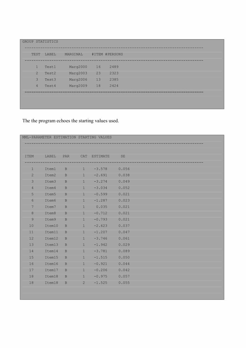
GROUP STATISTICS -------------------------------------------------------------------------------- TEST LABEL MARGINAL #ITEM #PERSONS -------------------------------------------------------------------------------- 1 Test1 Marg2000 16 2489 2 Test2 Marg2003 23 2323 3 Test3 Marg2006 13 2385 4 Test4 Marg2009 18 2424 ================================================================================

The the program echoes the starting values used.

MML-PARAMETER ESTIMATION STARTING VALUES -------------------------------------------------------------------------------- ITEM LABEL PAR CAT ESTIMATE SE -------------------------------------------------------------------------------- 1 Item1 B 1 -3.578 0.056 2 Item2 B 1 -2.691 0.038 3 Item3 B 1 -3.274 0.049 4 Item4 B 1 -3.034 0.052 5 Item5 B 1 -0.599 0.021 6 Item6 B 1 -1.287 0.023 7 Item7 B 1 0.035 0.021 8 Item8 B 1 -0.712 0.021 9 Item9 B 1 -0.793 0.021 10 Item10 B 1 -2.623 0.037 11 Item11 B 1 -1.207 0.047 12 Item12 B 1 -3.746 0.061 13 Item13 B 1 -1.942 0.029 14 Item14 B 1 -3.781 0.089 15 Item15 B 1 -1.515 0.050 16 Item16 B 1 -0.921 0.044 17 Item17 B 1 -0.206 0.042 18 Item18 B 1 -0.975 0.057 18 Item18 B 2 -1.525 0.055

The program proceeds with the estimation of the 1PLM/PCM and then with the

2PLM/3PLM/GPCM estimation. In the output, the former models are referred to as Rasch-Type

models, the latter as Lord-type models. First the iteration istory is displayed.

================================================================================ ANALYSES USING RASCH-TYPE MODELS: 1PL AND PCM ================================================================================ MML ITERATION HISTORY -------------------------------------------------------------------------------- 1 541.72420 RASCH-MODEL time: min. 0 | sec. 0.71 -93064.519 2 55.60175 RASCH-MODEL time: min. 0 | sec. 0.71 -93008.918 3 23.99087 RASCH-MODEL time: min. 0 | sec. 0.70 -92984.927 4 12.12134 RASCH-MODEL time: min. 0 | sec. 0.72 -92972.805 5 6.24537 RASCH-MODEL time: min. 0 | sec. 0.70 -92966.560 6 3.23526 RASCH-MODEL time: min. 0 | sec. 0.71 -92963.325 7 1.68386 RASCH-MODEL time: min. 0 | sec. 0.70 -92961.641 8 0.88554 RASCH-MODEL time: min. 0 | sec. 0.72 -92960.755 9 0.47543 RASCH-MODEL time: min. 0 | sec. 0.70 -92960.280 10 0.26440 RASCH-MODEL time: min. 0 | sec. 0.72 -92960.015 ……………………………….. ……………………………….. ……………………………….. 88 0.00000 RASCH-MODEL time: min. 0 | sec. 0.70 -92959.397 89 0.00000 RASCH-MODEL time: min. 0 | sec. 0.73 -92959.397 90 0.00000 RASCH-MODEL time: min. 0 | sec. 0.72 -92959.397 91 0.00000 RASCH-MODEL time: min. 0 | sec. 0.71 -92959.397 92 0.00000 RASCH-MODEL time: min. 0 | sec. 0.72 -92959.397 93 0.00000 RASCH-MODEL time: min. 0 | sec. 0.70 -92959.397 94 0.00000 RASCH-MODEL time: min. 0 | sec. 0.70 -92959.397 95 0.00000 RASCH-MODEL time: min. 0 | sec. 0.72 -92959.397 96 0.00000 RASCH-MODEL time: min. 0 | sec. 0.70 -92959.397 97 0.00000 RASCH-MODEL time: min. 0 | sec. 0.71 -92959.397 98 0.00000 RASCH-MODEL time: min. 0 | sec. 0.72 -92959.397 99 0.00000 RASCH-MODEL time: min. 0 | sec. 0.70 -92959.397 100 0.00000 RASCH-MODEL time: min. 0 | sec. 0.72 -92959.397 --------------------------------------------------------------------------------

The category bounds parameters refer to parameterization (21), the transformed parameters refer to

(20).

MML-PARAMETER ESTIMATION RASCH-TYPE-MODEL -------------------------------------------------------------------------------- CATEGORY BOUNDS TRANSFORMED ITEM LABEL PAR CAT ESTIMATE SE ESTIMATE SE -------------------------------------------------------------------------------- 1 Item1 B 1 -3.930 0.062 -3.930 0.062 2 Item2 B 1 -2.989 0.045 -2.989 0.045 3 Item3 B 1 -3.611 0.055 -3.611 0.055 4 Item4 B 1 -3.341 0.064 -3.341 0.064 5 Item5 B 1 -0.658 0.029 -0.658 0.029 6 Item6 B 1 -1.441 0.034 -1.441 0.034 7 Item7 B 1 0.071 0.031 0.071 0.031 8 Item8 B 1 -0.789 0.031 -0.789 0.031 9 Item9 B 1 -0.881 0.030 -0.881 0.030 10 Item10 B 1 -2.917 0.045 -2.917 0.045 11 Item11 B 1 -1.016 0.057 -1.016 0.057 12 Item12 B 1 -4.106 0.069 -4.106 0.069 13 Item13 B 1 -2.173 0.035 -2.173 0.035 14 Item14 B 1 -3.772 0.095 -3.772 0.095 15 Item15 B 1 -1.353 0.057 -1.353 0.057 16 Item16 B 1 -0.704 0.053 -0.704 0.053 17 Item17 B 1 0.086 0.054 0.086 0.054 18 Item18 B 1 -1.534 0.062 -1.534 0.062 18 Item18 B 2 -0.798 0.050 -2.332 0.073 18 Item18 B 3 -1.524 0.039 -3.856 0.083 19 Item19 B 1 -3.455 0.128 -3.455 0.128 19 Item19 B 2 -1.596 0.044 -5.050 0.130 19 Item19 B 3 -0.580 0.033 -5.631 0.136 20 Item20 B 1 -2.647 0.066 -2.647 0.066 20 Item20 B 2 -0.039 0.035 -2.687 0.077 20 Item20 B 3 0.162 0.037 -2.525 0.086 21 Item21 B 1 -2.577 0.058 -2.577 0.058 21 Item21 B 2 -0.308 0.033 -2.886 0.066 21 Item21 B 3 1.335 0.042 -1.551 0.082 22 Item22 B 1 -3.200 0.128 -3.200 0.128 22 Item22 B 2 0.299 0.054 -2.901 0.137 22 Item22 B 3 1.421 0.073 -1.480 0.154 23 Item23 B 1 -2.310 0.043 -2.310 0.043 23 Item23 B 2 -0.117 0.031 -2.427 0.055 23 Item23 B 3 1.506 0.041 -0.921 0.074 --------------------------------------------------------------------------------

ESTIMATION OF POPULATION PARAMETERS -------------------------------------------------------------------------------- POPULATION : Marg2000 -------------------------------------------------------------------------------- MEAN : -0.550 STANDARD DEVIATION : 0.655 SE(MEAN) : 0.025 SE(STANDARD DEVIATION) : 0.015 -------------------------------------------------------------------------------- POPULATION : Marg2003 -------------------------------------------------------------------------------- MEAN : 0.005 STANDARD DEVIATION : 0.692 SE(MEAN) : 0.026 SE(STANDARD DEVIATION) : 0.016 -------------------------------------------------------------------------------- POPULATION : Marg2006 -------------------------------------------------------------------------------- MEAN : -0.341 STANDARD DEVIATION : 1.221 SE(MEAN) : 0.035 SE(STANDARD DEVIATION) : 0.026 -------------------------------------------------------------------------------- POPULATION : Marg2009 -------------------------------------------------------------------------------- MEAN : 0.000 STANDARD DEVIATION : 0.677 SE(MEAN) : 0.000 SE(STANDARD DEVIATION) : 0.017 -------------------------------------------------------------------------------- LOG-LIKELIHOOD -92959.397 -------------------------------------------------------------------------------- MEAN ML Estimates of Ability in Booklet 1 2482 -0.5191 MEAN ML Estimates of Ability in Booklet 2 2319 0.0357 MEAN ML Estimates of Ability in Booklet 3 2261 -0.4395 MEAN ML Estimates of Ability in Booklet 4 2412 0.0446 MEAN Weighted ML Estimates of Ability in Booklet 1 2490 -0.5433 MEAN Weighted ML Estimates of Ability in Booklet 2 2324 0.0022 MEAN Weighted ML Estimates of Ability in Booklet 3 2386 -0.3623 MEAN Weighted ML Estimates of Ability in Booklet 4 2425 -0.0035 MEAN EAP Estimates of Ability in Booklet 1 2489 -0.5503 MEAN EAP Estimates of Ability in Booklet 2 2323 0.0054 MEAN EAP Estimates of Ability in Booklet 3 2385 -0.3412 MEAN EAP Estimates of Ability in Booklet 4 2424 0.0000 ---------------------------------------------------- BOOKLET VAR(E(8|X)) E(VAR(8|X)) VAR(8) REL ---------------------------------------------------- 1 0.279 0.151 0.429 0.649 2 0.336 0.143 0.479 0.702 3 1.080 0.411 1.491 0.724 4 0.289 0.170 0.459 0.630 ----------------------------------------------------

The first table gives the score distribution and its posterior expectation. In the second table scores are

collapsed to create expected frequencies over 10.0. Lagrange multipliers ability distribution for RASCH-TYPE MODEL ================================================================================ Booklet : 1 -------------------------------------------- Score Frequency Expected ------------------------------------------- 0 1 0.00 1 0 0.05 2 0 0.24 3 0 0.77 4 1 1.84 ……………………………………. ……………………………………. 21 151 161.79 22 99 112.63 23 66 67.83 24 43 33.26 25 20 11.77 26 5 2.25 ------------------------------------------- Score Range Frequency Expected ------------------------------------------- 0 8 44 47.48 9 9 28 35.30 10 10 39 55.01 11 11 93 81.06 12 12 109 112.42 13 13 156 147.34 14 14 203 183.53 15 15 233 217.82 16 16 262 245.66 17 17 245 261.74 18 18 256 261.49 19 19 236 242.87 20 20 201 207.74 21 21 151 161.79 22 22 99 112.63 23 23 66 67.83 24 24 43 33.26 25 26 25 14.02 ------------------------------------------- LM df Prob Approx df Prob ------------------------------------------- 36.77 17 0.00 24.70 17 0.10 -------------------------------------------

.

The first LM test reported above uses the complete matrix of weights, the second one is a diagonal

approximation. The test is repeated for every booklet in the design.

Two DIF-tests are presented. The first panel below displays a test for the constancy of the

parameters of a certain item parameter against the same parameters in all other booklets. This test is

repeated for all booklets. The second panel displays a test which tests the constancy of item

parameters across all booklets.

In the example below, the focal group is booklet 1, and the reference group consists of all other

booklets. The columns labeled Obs and Exp give the average observed and posterior expected item

scores in the focal and reference group, respectively. The column labeled Abs Dif. Gives the

absolute difference between the two. The column labeled LM gives the value of the LM statistic, the

column labeled df gives the degrees of freedom and the column labeled Prob gives the significance

probability. Due to the large sample size, all tests are significant. Therefore, the column the absolute

differences are more informative with respect to model violations here.

For more information refer to Glas (1988, 1998, 1999), Glas & Suárez-Falćon, (2003) and Glas and

Verhelst (1989, 1995).

Lagrange tests DIF for RASCH-TYPE-MODEL for Booklet 1 -------------------------------------------------------------------------------- Focal-Group Reference Abs. Item LM df Prob Obs Exp Obs Exp Dif. -------------------------------------------------------------------------------- 1 Item1 7.83 1 0.01 0.97 0.96 0.96 0.97 0.01 2 Item2 0.27 1 0.60 0.91 0.91 0.93 0.93 0.00 3 Item3 46.18 1 0.00 0.97 0.95 0.95 0.96 0.01 5 Item5 295.30 1 0.00 0.65 0.52 0.57 0.62 0.09 6 Item6 1580.14 1 0.00 0.40 0.69 0.86 0.76 0.19 7 Item7 220.18 1 0.00 0.47 0.36 0.43 0.46 0.07 8 Item8 347.82 1 0.00 0.69 0.55 0.60 0.64 0.09 9 Item9 116.21 1 0.00 0.66 0.57 0.63 0.66 0.05 10 Item10 706.01 1 0.00 0.98 0.90 0.89 0.92 0.05 12 Item12 44.22 1 0.00 0.98 0.97 0.97 0.97 0.01 13 Item13 30.37 1 0.00 0.78 0.82 0.87 0.86 0.02 18 Item18 2995.19 3 0.00 1.55 2.14 2.82 2.51 0.45 19 Item19 147.61 3 0.00 2.35 2.22 2.41 2.47 0.09 20 Item20 449.10 3 0.00 1.35 1.56 2.01 1.91 0.16 21 Item21 303.87 3 0.00 1.62 1.45 1.63 1.72 0.13 23 Item23 458.96 3 0.00 1.59 1.35 1.49 1.57 0.16 --------------------------------------------------------------------------------

Lagrange tests DIF over all groups for RASCH-TYPE-MODEL ------------------------------------------------------------ Item LM df Prob Abs.Dif. ------------------------------------------------------------ 1 Item1 12.02 3 0.01 0.01 2 Item2 43.18 3 0.00 0.01 3 Item3 48.89 3 0.00 0.01 4 Item4 17.31 2 0.00 0.01 5 Item5 311.09 3 0.00 0.07 6 Item6 2092.59 3 0.00 0.15 7 Item7 255.18 3 0.00 0.06 8 Item8 378.54 3 0.00 0.07 9 Item9 178.40 3 0.00 0.05 10 Item10 711.79 3 0.00 0.04 12 Item12 62.03 3 0.00 0.01 13 Item13 39.67 3 0.00 0.02 14 Item14 12.70 1 0.00 0.01 18 Item18 2801.92 2 0.00 0.40 19 Item19 156.63 2 0.00 0.09 20 Item20 595.76 2 0.00 0.16 21 Item21 278.46 2 0.00 0.12 23 Item23 751.42 3 0.00 0.18 ------------------------------------------------------------

The test for the item characteristic curves generally follows the same lines as the tests for DIF. Only

here, observed and posterior expected are computed using a partitioning of respondents according to

their score level (i.e., the score level computed without the item targeted). Three score levels are

formed. The sample sizes within the score levels are displayed below in the three last columns.

Again, due to the sample size, the absolute difference between observed and expected average score

are more informative then the outcomes of the statistics.

For more information refer to Glas (1988, 1998, 1999), Glas & Suárez-Falćon, (2003) and Glas and

Verhelst (1989, 1995).

Lagrange multipliers tracelines for RASCH-TYPE MODEL ================================================================================ Booklet : 1 ---------------------------------------------------------------------------------------------- Groups: 1 2 3 Abs. 1 2 3 Item LM df Prob Obs. Exp. Obs. Exp. Obs. Exp. Dif. Size Size Size ---------------------------------------------------------------------------------------------- 1 Item1 10.47 2 0.01 0.94 0.94 0.98 0.96 0.99 0.98 0.01 869 763 825 2 Item2 1.16 2 0.56 0.85 0.86 0.91 0.91 0.97 0.95 0.01 837 781 834 3 Item3 32.15 2 0.00 0.95 0.92 0.97 0.95 0.99 0.97 0.02 867 766 824 5 Item5 149.74 2 0.00 0.46 0.39 0.69 0.52 0.80 0.65 0.13 766 795 882 6 Item6 1196.21 2 0.00 0.18 0.57 0.36 0.68 0.60 0.79 0.30 690 805 956 7 Item7 48.74 2 0.00 0.29 0.24 0.42 0.34 0.65 0.48 0.10 705 801 930 8 Item8 151.59 2 0.00 0.55 0.42 0.67 0.55 0.83 0.68 0.14 774 781 884 9 Item9 67.73 2 0.00 0.53 0.44 0.65 0.57 0.77 0.70 0.08 770 788 886 10 Item10 648.53 2 0.00 0.97 0.85 0.99 0.91 0.98 0.94 0.08 863 765 822 12 Item12 20.44 2 0.00 0.96 0.95 0.98 0.97 1.00 0.98 0.02 868 765 822 13 Item13 58.10 2 0.00 0.63 0.73 0.81 0.82 0.91 0.89 0.05 810 798 846 18 Item18 843.24 2 0.00 1.32 1.63 1.44 2.14 1.85 2.55 0.57 727 836 910 19 Item19 185.41 2 0.00 2.19 1.91 2.32 2.20 2.49 2.48 0.14 723 794 957 20 Item20 381.33 2 0.00 0.88 1.19 1.29 1.48 1.73 1.88 0.22 664 845 958 21 Item21 132.53 2 0.00 1.31 1.17 1.61 1.42 1.91 1.71 0.17 745 843 879 23 Item23 218.82 2 0.00 1.30 1.08 1.56 1.32 1.88 1.61 0.24 745 830 870 ----------------------------------------------------------------------------------------------

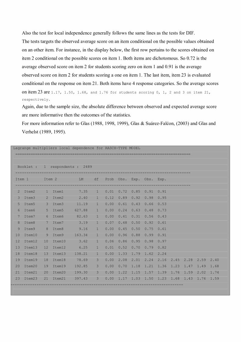
Also the test for local independence generally follows the same lines as the tests for DIF.

The tests targets the observed average score on an item conditional on the possible values obtained

on an other item. For instance, in the display below, the first row pertains to the scores obtained on

item 2 conditional on the possible scores on item 1. Both items are dichotomous. So 0.72 is the

average observed score on item 2 for students scoring zero on item 1 and 0.91 is the average

observed score on item 2 for students scoring a one on item 1. The last item, item 23 is evaluated

conditional on the response on item 21. Both items have 4 response categories. So the average scores

on item 23 are 1.17, 1.50, 1.68, and 1.76 for students scoring 0, 1, 2 and 3 on item 21, respectively. Again, due to the sample size, the absolute difference between observed and expected average score

are more informative then the outcomes of the statistics.

For more information refer to Glas (1988, 1998, 1999), Glas & Suárez-Falćon, (2003) and Glas and

Verhelst (1989, 1995).

Lagrange multipliers local dependence for RASCH-TYPE MODEL ================================================================================ Booklet : 1 respondents : 2489 -------------------------------------------------------------------------------- Item 1 Item 2 LM df Prob Obs. Exp. Obs. Exp. -------------------------------------------------------------------------------- 2 Item2 1 Item1 7.35 1 0.01 0.72 0.85 0.91 0.91 3 Item3 2 Item2 2.40 1 0.12 0.89 0.92 0.98 0.95 5 Item5 3 Item3 11.19 1 0.00 0.61 0.43 0.66 0.53 6 Item6 5 Item5 627.88 1 0.00 0.24 0.63 0.48 0.73 7 Item7 6 Item6 82.63 1 0.00 0.41 0.31 0.56 0.43 8 Item8 7 Item7 3.19 1 0.07 0.48 0.50 0.92 0.61 9 Item9 8 Item8 9.16 1 0.00 0.45 0.50 0.75 0.61 10 Item10 9 Item9 163.34 1 0.00 0.96 0.88 0.99 0.91 12 Item12 10 Item10 3.62 1 0.06 0.86 0.95 0.98 0.97 13 Item13 12 Item12 6.25 1 0.01 0.52 0.70 0.79 0.82 18 Item18 13 Item13 138.21 1 0.00 1.33 1.79 1.62 2.24 19 Item19 18 Item18 78.69 3 0.00 2.08 2.01 2.24 2.16 2.45 2.28 2.59 2.40 20 Item20 19 Item19 192.85 3 0.00 0.70 1.18 1.21 1.36 1.23 1.47 1.49 1.68 21 Item21 20 Item20 199.30 3 0.00 1.22 1.15 1.57 1.39 1.76 1.59 2.02 1.74 23 Item23 21 Item21 397.43 3 0.00 1.17 1.03 1.50 1.23 1.68 1.43 1.76 1.59

--------------------------------------------------------------------------------

All output tables are repeated for Lord-type models. For instance, the table with parameter estimates

looks as follows.

MML-PARAMETER ESTIMATION LORD-TYPE-MODEL -------------------------------------------------------------------------------- CATEGORY BOUNDS TRANSFORMED ITEM LABEL PAR CAT ESTIMATE SE ESTIMATE SE -------------------------------------------------------------------------------- 1 Item1 A 0 0.813 0.061 1 Item1 B 1 -4.046 0.004 -4.046 0.098 2 Item2 A 0 0.771 0.049 2 Item2 B 1 -3.047 0.010 -3.047 0.067 3 Item3 A 0 0.825 0.058 3 Item3 B 1 -3.741 0.002 -3.741 0.087 4 Item4 A 0 1.287 0.088 4 Item4 B 1 -4.005 0.005 -4.005 0.152 5 Item5 A 0 0.653 0.031 5 Item5 B 1 -0.636 0.003 -0.636 0.031 19 Item19 A 0 0.301 0.021 19 Item19 B 1 -2.765 0.009 -2.765 0.128 19 Item19 B 2 -1.205 0.005 -3.971 0.130 19 Item19 B 3 -0.509 0.005 -4.480 0.133 20 Item20 A 0 1.079 0.043 20 Item20 B 1 -3.293 0.017 -3.293 0.100 20 Item20 B 2 -0.264 0.002 -3.558 0.128 20 Item20 B 3 0.336 0.003 -3.222 0.136 21 Item21 A 0 0.471 0.023 21 Item21 B 1 -2.308 0.013 -2.308 0.063 21 Item21 B 2 -0.227 0.014 -2.535 0.071 21 Item21 B 3 1.221 0.005 -1.315 0.079 22 Item22 A 0 0.609 0.048 22 Item22 B 1 -3.042 0.003 -3.042 0.137 22 Item22 B 2 0.356 0.004 -2.687 0.144 22 Item22 B 3 1.381 0.003 -1.306 0.153 23 Item23 A 0 0.511 0.021 23 Item23 B 1 -2.011 0.010 -2.011 0.048 23 Item23 B 2 -0.058 0.005 -2.069 0.058 23 Item23 B 3 1.344 0.001 -0.725 0.068 --------------------------------------------------------------------------------

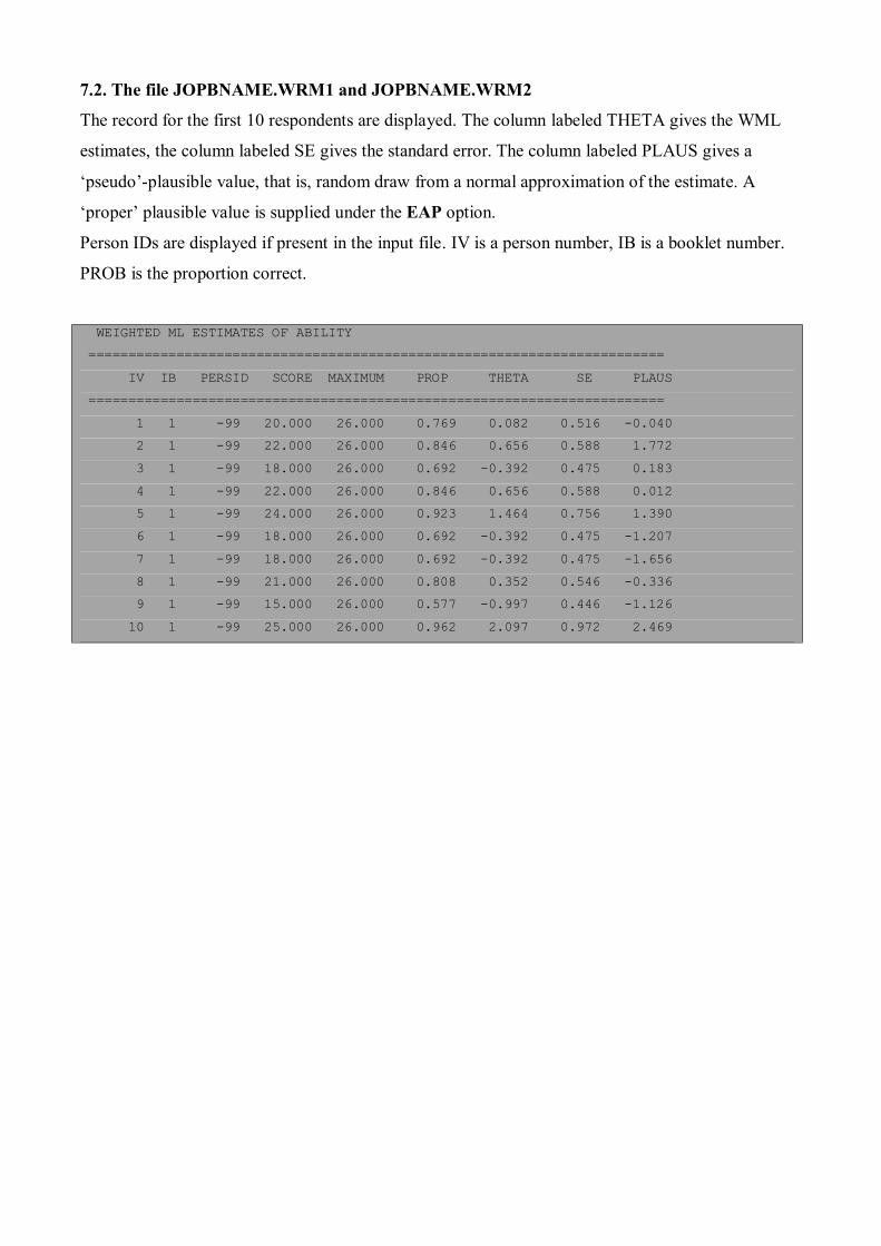
7.2. The file JOPBNAME.WRM1 and JOPBNAME.WRM2

The record for the first 10 respondents are displayed. The column labeled THETA gives the WML

estimates, the column labeled SE gives the standard error. The column labeled PLAUS gives a

‘pseudo’-plausible value, that is, random draw from a normal approximation of the estimate. A

‘proper’ plausible value is supplied under the EAP option.

Person IDs are displayed if present in the input file. IV is a person number, IB is a booklet number.

PROB is the proportion correct.

WEIGHTED ML ESTIMATES OF ABILITY ======================================================================== IV IB PERSID SCORE MAXIMUM PROP THETA SE PLAUS ======================================================================== 1 1 -99 20.000 26.000 0.769 0.082 0.516 -0.040 2 1 -99 22.000 26.000 0.846 0.656 0.588 1.772 3 1 -99 18.000 26.000 0.692 -0.392 0.475 0.183 4 1 -99 22.000 26.000 0.846 0.656 0.588 0.012 5 1 -99 24.000 26.000 0.923 1.464 0.756 1.390 6 1 -99 18.000 26.000 0.692 -0.392 0.475 -1.207 7 1 -99 18.000 26.000 0.692 -0.392 0.475 -1.656 8 1 -99 21.000 26.000 0.808 0.352 0.546 -0.336 9 1 -99 15.000 26.000 0.577 -0.997 0.446 -1.126 10 1 -99 25.000 26.000 0.962 2.097 0.972 2.469

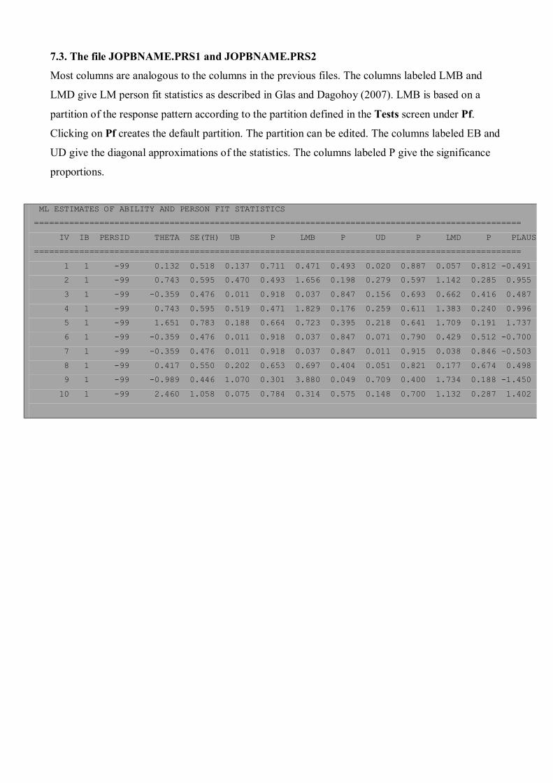
7.3. The file JOPBNAME.PRS1 and JOPBNAME.PRS2

Most columns are analogous to the columns in the previous files. The columns labeled LMB and

LMD give LM person fit statistics as described in Glas and Dagohoy (2007). LMB is based on a

partition of the response pattern according to the partition defined in the Tests screen under Pf.

Clicking on Pf creates the default partition. The partition can be edited. The columns labeled EB and

UD give the diagonal approximations of the statistics. The columns labeled P give the significance

proportions.

ML ESTIMATES OF ABILITY AND PERSON FIT STATISTICS ================================================================================================= IV IB PERSID THETA SE(TH) UB P LMB P UD P LMD P PLAUS ================================================================================================= 1 1 -99 0.132 0.518 0.137 0.711 0.471 0.493 0.020 0.887 0.057 0.812 -0.491 2 1 -99 0.743 0.595 0.470 0.493 1.656 0.198 0.279 0.597 1.142 0.285 0.955 3 1 -99 -0.359 0.476 0.011 0.918 0.037 0.847 0.156 0.693 0.662 0.416 0.487 4 1 -99 0.743 0.595 0.519 0.471 1.829 0.176 0.259 0.611 1.383 0.240 0.996 5 1 -99 1.651 0.783 0.188 0.664 0.723 0.395 0.218 0.641 1.709 0.191 1.737 6 1 -99 -0.359 0.476 0.011 0.918 0.037 0.847 0.071 0.790 0.429 0.512 -0.700 7 1 -99 -0.359 0.476 0.011 0.918 0.037 0.847 0.011 0.915 0.038 0.846 -0.503 8 1 -99 0.417 0.550 0.202 0.653 0.697 0.404 0.051 0.821 0.177 0.674 0.498 9 1 -99 -0.989 0.446 1.070 0.301 3.880 0.049 0.709 0.400 1.734 0.188 -1.450 10 1 -99 2.460 1.058 0.075 0.784 0.314 0.575 0.148 0.700 1.132 0.287 1.402

7.4. The file JOPBNAME.EAP1 and JOPBNAME.EAP2

The column labeled EAP(T) gives the posterior expectation, the column labeled POST(T) gives the

posterior standard deviation. The column labeled PLAUS gives a plausible value, that is, random

draw from the posterior distribution.

EAP ESTIMATES OF ABILITY ======================================================================== IV IB PERSID SCORE MAXIMUM PROP EAP(T) POST(T) PLAUS ======================================================================== 1 1 -99 20.000 26.000 0.769 -0.106 0.397 -0.174 2 1 -99 22.000 26.000 0.846 0.221 0.412 0.277 3 1 -99 18.000 26.000 0.692 -0.411 0.385 -0.071 4 1 -99 22.000 26.000 0.846 0.221 0.412 0.135 5 1 -99 24.000 26.000 0.923 0.577 0.432 0.819 6 1 -99 18.000 26.000 0.692 -0.411 0.385 -0.572 7 1 -99 18.000 26.000 0.692 -0.411 0.385 -0.352 8 1 -99 21.000 26.000 0.808 0.055 0.404 0.225 9 1 -99 15.000 26.000 0.577 -0.843 0.374 -0.976 10 1 -99 25.000 26.000 0.962 0.768 0.443 0.588

Bibliography Ackerman, T.A. (1996a). Developments in multidimensional item response theory. Applied Psychological Measurement

20, 309-310. Ackerman, T.A. (1996b). Graphical representation of multidimensional item response theory analyses. Applied

Psychological Measurement 20, 311-329. Adams, R.J., & Wilson, M.R. (1996). A random coefficients multinomial logit: A generalized approach to fitting Rasch

models. In G.Engelhard and M. Wilson, (Eds.), Objective measurement: Theory into practice, Vol. 3 (pp.143-166). Nordwood, NJ: Ablex Publishing Corporation.

Adams, R.J., Wilson, M.R., & Wang, W.C. (1997). The random coefficients multinomial logit. Applied Psychological Measurement, 21, 1-25.

Adams, R.J., Wilson, M.R., & Wu, M. (1997). Multilevel item response theory models: an approach to errors in variables of regression. Journal of Educational and Behavioral Statistics, 22, 47-76.

Adema, J.J., & van der Linden, W.J. (1989). Algorithms for computerized test construction using classical item parameters. Journal of Educational Statistics, 14, 279-290.

Aitchison, J., & Silvey, S.D. (1958). Maximum likelihood estimation of parameters subject to restraints. Annals of Mathematical Statistics 29, 813-828.

Aitkin, M., Anderson, D., & Hinde, J. (1981). Statistical modeling of data on teaching styles. Journal of the Royal Statistical Society, Series A (General), 149, 1-43.

Albert, J.H. (1992). Bayesian estimation of normal ogive item response functions using Gibbs sampling. Journal of Educational Statistics, 17, 251-269.

Andersen, E.B. (1977). Sufficient statistics and latent trait models. Psychometrika, 42, 69-81. Anderson L.W. & Bourke, S.F. (2000). Assessing affective characteristics in the schools. Mahwah, NJ: Lawrence

Erlbaum. Béguin, A.A., & Glas, C.A.W. (2001). MCMC estimation and some fit analysis of multidimensional IRT models.

Psychometrika, 66, 541-562. Birnbaum, A. (1968). Some latent trait models. In F.M. Lord & M.R. Novick (Eds.), Statistical theories of mental test

scores. Reading, MA: Addison-Wesley. Bock, R.D. (1972). Estimating item parameters and latent ability when responses are scored in two or more nominal

categories. Psychometrika, 37, 29-51. Bock, R.D., & Aitkin, M. (1981). Marginal maximum likelihood estimation of item parameters: an application of an

EM-algorithm. Psychometrika, 46, 443-459. Bock, R.D., Gibbons, R.D., & Muraki, E. (1988). Full-information factor analysis. Applied Psychological Measurement

12, 261-280. Bradlow, E.T., Wainer, H., & Wang, X. (1999). A Bayesian random effects model for testlets. Psychometrika, 64, 153-

168. Camilli, G., & Shepard, L.A. (1994). Methods for Identifying Biased Test Items. Thousand Oaks, CA: Sage. Dempster, A.P., Laird, N.M., & Rubin, D.B. (1977). Maximum likelihood from incomplete data via the EM algorithm

(with discussion). Journal of the Royal Statistical Society B, 39, 1-38. Efron, B. (1979). Bootstrap methods: Another look at the jackknife. Annals of Statistics, 7, 1-26. Efron, B., & Gong, G. (1983). A leisurely look at the bootstrap, the jackknife, and the cross-validation. The American

Statistician, 37, 36-49. Emons, W.H.M. (1998). Nonequivalent Groups IRT Observed Score Equating. Its Applicability and Appropriateness for

the Swedish Scholastic Aptitude Test. Twente University. Fischer, G.H. (1974). Einführung in die theorie psychologischer tests: Introduction to the theory of psychological tests.

Bern: Huber. Fischer, G.H. (1995). Some neglected problems in IRT. Psychometrika, 60, 459-487. Fischer, G.H., & Molenaar, I.W. (1995). Rasch models. Their foundation, recent developments and applications. New

York, NJ: Springer. Fischer, G.H., & Scheiblechner, H.H. (1970). Algorithmen und Programme für das probabilistische Testmodell von

Rasch. Psychologische Beiträge, 12, 23-51. Fox, J.P., & Glas, C.A.W. (2001). Bayesian Estimation of a Multilevel IRT Model using Gibbs Sampling.

Psychometrika, 66, 271-288. Fox, J.P., & Glas, C.A.W. (2002). Modeling measurement error in structural multilevel models. In G.A. Marcoulides and

I. Moustaki (Eds.). Latent Variable and Latent Structure models. Mahwah, NJ: Laurence Erlbaum. Fraser, C. (1988). NOHARM: A Computer Program for Fitting Both Unidimensional and Multidimensional Normal

Ogive Models of Latent Trait Theory. (Computer Software). NSW: University of New England. Fuller, W.A. (1987). Measurement Error Models. New York, NJ: Wiley. Gelfand, A.E., & Smith, A.F.M. (1990). Sampling-based approaches to calculating marginal densities. Journal of the

American Statistical Association, 85, 398-409.

Glas, C.A.W. (1988a). The derivation of some tests for the Rasch model from the multinomial distribution. Psychometrika, 53, 525-546.

Glas, C.A.W. (1988b). The Rasch model and multi-stage testing. Journal of Educational Statistics, 13, 45-52. Glas, C.A.W. (1992). A Rasch model with a multivariate distribution of ability. In M. Wilson (Ed.), Objective

Measurement: Theory into practice, Vol. 1 (pp. 236-258), New Jersey, NJ: Ablex Publishing Corporation. Glas, C.A.W. (1997). Towards an integrated testing service system. European Journal of Psychological Assessment, 13,

38-48. Glas, C.A.W. (1998) Detection of differential item functioning using Lagrange multiplier tests. Statistica Sinica, 8, 647-

667. Glas, C.A.W. (1999). Modification indices for the 2-pl and the nominal response model. Psychometrika, 64, 273-294. Glas, C.A.W. en Béguin, A.A. (1996). Appropriateness of IRT observed score equating. OMD Research Reports, 96-4,

Twente University. Glas, C.A.W., & Suárez-Falćon, J.C. (2003). A comparison of item-fit statistics for the three-parameter logistic model.

Applied Psychological Measurement, 27, 87-106. Glas, C.A.W., and Verhelst, N.D. (1989). Extensions of the partial credit model. Psychometrika, 54, 635-659. Glas, C.A.W., & Verhelst, N.D. (1995). Tests of fit for polytomous Rasch models. In G.H. Fischer & I.W. Molenaar

(Eds.), Rasch models: foundations, recent developments and applications. (pp.325-352). New York, NJ: Springer.

Glas, C.A.W., & van der Linden, W.J. (2003). Computerized adaptive testing with item cloning. Applied Psychological Measurement, 27, 256-272.

Glas, C.A.W., & van der Linden, W.J. (2001). Modeling Variability in Item Parameters in Educational Measurement. Twente University, OMD Research Report 01-11.

Glas, C.A.W., Wainer, H., & Bradlow (2000). MML and EAP estimates for the testlet response model. In W.J. van der Linden & C.A.W. Glas (Eds.), Computer Adaptive Testing: Theory and Practice (pp.271-287). Boston MA: Kluwer-Nijhoff Publishing.

Goldstein, H. (1986). Multilevel mixed linear models analysis using iterative generalized least squares. Biometrika, 73, 43-56.

Gulliksen, H. (1950). Theory of mental tests. New York, NJ: Wiley. Hambleton, R.K., & Rogers, H.J. (1989). Detecting potentially biased test items: comparison of IRT area and Mantel-

Haenszel methods. Applied Measurement in Education, 2, 313-334. Hambleton, R.K., & Swaminathan, H. (1985). Item response theory: Principles and applications (2nd ed.). Boston:

Kluwer-Nijhoff Publishing. Hambleton, R.K., Swaminathan, H., & Rogers, H.J. (1991). Fundaments of item response theory. Newbury Park, CA:

Sage. Hendrawan, I., Glas, C.A.W., & Meijer, R.R. (2001). The Effect of Person Misfit on Classification Decisions. Research

Report 01-05, Faculty of Educational Science and Technology, University of Twente, the Netherlands. Holland, P.W. en Rubin, D.B. (1982). Test Equating. New York: Academic Press. Holland, P.W. and Thayer, D.T. (1988). Differential item functioning and the Mantel-Haenszel procedure. In H. Wainer

and H.I. Braun (Eds.), Test validity. Hillsdale, NJ: Lawrence Erlbaum Associates Inc. Holland, P.W., & Wainer, H. (1993). Differential Item Functioning. Hillsdale, N.J., Erlbaum. Janssen, R., Tuerlinckx, F., Meulders, M. & de Boeck, P. (2000). A hierarchical IRT model for criterion-referenced

measurement. Journal of Educational and Behavioral Statistics, 25, 285-306. Johnson, V.E., & Albert, J.H. (1999). Ordinal data modeling. New York, NJ: Springer. Jöreskog, K.G. & D. Sörbom, (1996). LISREL. (Computer Software). Chicago, IL: Scientific Software International, Inc. Kelderman, H. (1984). Loglinear RM tests. Psychometrika, 49, 223-245. Kelderman, H. (1989). Item bias detection using loglinear IRT. Psychometrika, 54, 681-697. Kiefer, J., & Wolfowitz, J. (1956). Consistency of the maximum likelihood estimator in the presence of infinitely many

incidental parameters. Annals of Mathematical Statistics, 27, 887-903. Kok, F.G., Mellenbergh, G.J., & van der Flier, H. (1985). Detecting experimentally induced item bias using the iterative

logit method. Journal of Educational Measurement, 22, 295-303. Kolen, M.J. en Brennan, R.L. (1995). Test Equating. New York: Springer. Lawley, D. N. (1943). On problems connected with item selection and test construction. Proceedings of the Royal

Society of Edinburgh, 61, 273-287. Lawley, D. N. (1944). The factorial analysis of multiple test items. Proceedings of the Royal Society of Edinburgh, 62-A,

74-82. Longford, N.T. (1987). A fast scoring algorithm for maximum likelihood estimation in unbalanced mixed models with

nested random factors. Biometrika, 74, 817-827. Longford, N.T. (1993). Random Coefficients Models. Oxford: Clarendon Press. Lord, F. M. (1952). A theory of test scores. Psychometric Monograph 7. Lord, F.M. (1953a). An application of confidence intervals and of maximum likelihood to the estimation of an

examinee's ability. Psychometrika, 18, 57-75.

Lord, F. M. (1953b). The relation of test score to the trait underlying the test. Educational and Psychological Measurement, 13, 517-548.

Lord, F.M. (1980). Applications of item response theory to practical testing problems. Hillsdale, N.J., Erlbaum. Lord, F.M. and Novick, M.R. (1968). Statistical theories of mental test scores. Reading: Addison-Wesley. Masters, G.N. (1982). A Rasch model for partial credit scoring. Psychometrika, 47, 149-174. McDonald, R.P. (1967). Nonlinear factor analysis. Psychometric monographs, No.15. Mellenbergh, G.J. (1995). Conceptual notes on models for discrete polytomous item responses. Applied Psychological

Measurement, 19, 91-100. McDonald, R.P. (1982). Linear versus nonlinear models in latent trait theory. Applied Psychological Measurement, 6,

379-396. Mislevy, R.J. (1984). Estimating latent distributions. Psychometrika, 49, 359-381. Mislevy, R.J. (1986). Bayes modal estimation in item response models. Psychometrika, 51, 177-195. Mislevy, R.J., & Bock, R.D. (1989). A hierarchical item-response model for educational testing. In R.D. Bock (Ed.),

Multilevel analysis of educational data. San Diego: Academic Press. Mislevy, R.J., & Bock, R.D. (1990). PC-BILOG. Item analysis and test scoring with binary logistic models. Mooresville,

IN: Scientific Software. Mislevy, R.J., Steinberg, L.S., & Almond, R.G. (2003). On the structure of educational assessments. Measurement, 1, 3-

62. Molenaar, I.W. (1995). Estimation of item parameters. In: G.H. Fischer, & I.W. Molenaar (Eds.), Rasch models:

Foundations, recent developments and applications. New York, NJ: Springer. Muraki, E. (1992). A generalized partial credit model: application of an EM algorithm. Applied Psychological

Measurement, 16, 159- 176. Muthén, B. (1984). A general structural equation model with dichotomous, ordered, categorical, and continuous latent

variable indicators. Psychometrika, 49, 115-132. Muthén, B. (1987). LISCOMP. (Computer Software). Neyman, J., and Scott, E.L. (1948). Consistent estimates, based on partially consistent observations. Econometrica, 16,

1-32. Nissan, S. (1999, April). Incorporating sound, visuals, and text for TOEFL on computer. Paper presented at the annual

meeting of the National Council on Measurement in Education, Montreal, Canada. Orlando, M., & Thissen, D. (2000). Likelihood-based item-fit indices for dichotomous item response theory models.

Applied Psychological Measurement, 24, 50-64. Patz, R. J., & Junker, B. W. (1999a). A straightforward approach to Markov chain Monte Carlo methods for item

response models. Journal of Educational and Behavioral Statistics, 24, 146-178. Patz, R. J., & Junker, B. W. (1999b). Applications and extensions of MCMC in IRT: Multiple Item Types, Missing Data,

and rated responses. Journal of Educational and Behavioral Statistics, 24, 342-366. Rao, C.R. (1947). Large sample tests of statistical hypothesis concerning several parameters with applications to

problems of estimation. Proceedings of the Cambridge Philosophical Society, 44, 50-57. Rasch, G. (1960). Probabilistic models for some intelligence and attainment tests. Copenhagen: Danish Institute for

Educational Research. Raudenbush, S.W., & Bryk, A. (1986). A hierarchical model for studying school effects. Sociology of Education, 59, 1-

17. Reckase, M.D. (1985). The difficulty of test items that measure more than one ability. Applied Psychological

Measurement, 9, 401-412. Reckase, M.D. (1997). A linear logistic multidimensional model for dichotomous item response data. In W.J. van der

Linden and R.K. Hambleton (Eds.), Handbook of modern item response theory. (pp.271-286). New York, NJ: Springer.

Rubin, D.B. (1976). Inference and missing data. Biometrika, 63, 581-592. Samejima, F. (1969). Estimation of latent ability using a pattern of graded scores. Psychometrika, Monograph

Supplement, No. 17. Shi, J. Q., & Lee, S. Y. (1998). Bayesian sampling based approach for factor analysis models with continuous and

polytomous data. British Journal of Mathematical and Statistical Psychology, 51, 233-252. Sireci, S.G., Wainer, H., & Thissen, D. (1991). On the reliability of testlet-based tests. Journal of Educational

Measurement, 28, 237-247. Snijders, T. (2001). Asymptotic distribution of person-fit statistics with estimated person parameter. Psychometrika, 66,

331-342. Swaminathan, H., & Rogers, H.J. (1990). Detecting differential item functioning using logistic regression procedures.

Journal of Educational Measurement, 27, 361-370. Takane, Y., & de Leeuw, J. (1987). On the relationship between item response theory and factor analysis of discretized

variables. Psychometrika, 52, 393-408. Thissen, D. (1982). Marginal maximum likelihood estimation for the one-parameter logistic model. Psychometrika, 47,

175-186.

Thissen, D. (1991). MULTILOG. Multiple, categorical item analysis and test scoring using item response theory. Chicago, IL: Scientific Software International, Inc.

Thissen, D., Steinberg, L., & Wainer, H. (1993). Detection of differential item functioning using the parameters of IRT models. In P.W. Holland & H. Wainer (Eds.), Differential Item Functioning (pp.67-113). Hillsdale, N.J., Erlbaum.

Thurstone, L.L. (1947). Multiple factor analysis. Chicago, IL: University of Chicago Press. Tutz, G. (1990). Sequential item response models with an ordered response. British Journal of Mathematical and

Statistical Psychology, 43, 39-55. Van den Wollenberg, A.L. (1982). Two new tests for the Rasch model. Psychometrika, 47, 123-140. Van der Linden, W.J., & Boekkooi-Timminga, E. (1988). A zero-one programming approach to Gulliksen’s matched

random subsets method. Applied Psychological Measurement, 12, 201-209. Van der Linden, W.J., & Boekkooi-Timminga, E. (1989). A maximin model for test design with practical constraints.

Psychometrika, 53, 237-247. Verhelst, N.D., & Glas, C.A.W. (1995). The generalized one parameter model: OPLM. In G.H. Fischer & I.W. Molenaar

(Eds.), Rasch models: their foundations, recent developments and applications. New York, NJ: Springer. Verhelst, N.D., Glas, C.A.W., & Verstralen, H.H.F.M. (1995). OPLM: computer program and manual. Arnhem: Cito,

the National Institute for Educational Measurement in the Netherlands. Verhelst, N.D., Glas, C.A.W., & de Vries, H.H. (1997). A steps model to analyze partial credit. In: W.J. van der Linden

and R.K. Hambleton (Eds.), Handbook of modern item response theory. (pp. 123-138). New York, NJ: Springer. Verschoor, A.J., & Straetmans, G.J.J.M. (2000). MATHCAT: A flexible testing system in mathematics education for

adults. In: W.J. van der Linden & C.A.W. Glas (Eds.), Computer Adaptive Testing: Theory and Practice (pp. 101-116). Boston: Kluwer-Nijhoff Publishing.

Wainer, H. (1995). Precision and differential item functioning on a testlet-based test: The 1991 Law School Admissions Test as an example. Applied Measurement in Education, 8, 157-187.

Wainer, H, Bradlow, E.T., & Du, Z. (2000). Testlet Response Theory: an Analogue for the 3-PL Useful in Testlet-Based Adaptive Testing. In W.J. van der Linden & C.A.W. Glas (Eds.), Computer Adaptive Testing: Theory and Practice (pp. 245-269). Boston: Kluwer-Nijhoff Publishing.

Wainer, H., & Kiely, G. (1987). Item clusters and computerized adaptive testing: A case for testlets. Journal of Educational Measurement, 24, 185-202.

Wainer, H. & Thissen, D. (1996). How is reliability related to the quality of test scores? What is the effect of local dependence on reliability? Educational Measurement: Issues and Practice, 15(1), 22-29.

Warm, T.A. (1989). Weighted likelihood estimation of ability in item response theory. Psychometrika, 54, 427-450. Wilson, D.T., Wood, R., & Gibbons, R. (1991). TESTFACT: Test scoring, Item statistics, and Item Factor Analysis.

[Computer Software]. Chicago, IL: Scientific Software International, Inc. Wilson, M., & Masters, G.N. (1993). The partial credit model and null categories. Psychometrika, 58, 85-99. Wright, B.D., & Panchapakesan, N. (1969). A procedure for sample- free item analysis. Educational and Psychological

Measurement, 29, 23-48. Wright, B.D., & Stone, M.H. (1979). Best Test Design. Chicago, IL: MESA Press University of Chicago. Wu, M.L., Adams, R.J., & Wilson, M.R. (1997). ConQuest: Generalized Item Response Modeling Software. (Computer

Software). Australian Council for Educational Research. Yen, W. (1981). Using simultaneous results to choose a latent trait model. Applied Psychological Measurement, 5, 245-

262. Yen, W. (1984). Effects of local item dependence on the fit and equating performance of the three-parameter logistic

model. Applied Psychological Measurement, 8, 125-145. Yen, W. (1993). Scaling performance assessments: Strategies for managing local item dependence. Journal of

Educational Measurement, 30, 187-213. Zimowski, M.F., Muraki, E., Mislevy, R.J., & Bock, R.D. (1996). Bilog MG: Multiple-Group IRT Analysis and Test

Maintenance for Binary Items. Chicago, IL: Scientific Software International, Inc.