Beaver Wood Pownal 248 Filing: No. 3 Motion for Preliminary Approval SD

Preliminary long-term forecasts of wood product demand in Australia Mihir Gupta, Kristen Corrie, Beau Hug and Kevin Burns
Research by the Australian Bureau of Agricultural
and Resource Economics and Sciences
Research report 13.6 May 2013

ii
© Commonwealth of Australia 2013 Ownership of intellectual property rights Unless otherwise noted, copyright (and any other intellectual property rights, if any) in this publication is owned by the Commonwealth of Australia (referred to as the Commonwealth). Creative Commons licence All material in this publication is licensed under a Creative Commons Attribution 3.0 Australia Licence, save for content supplied by third parties, logos and the Commonwealth Coat of Arms.
Creative Commons Attribution 3.0 Australia Licence is a standard form licence agreement that allows you to copy, distribute, transmit and adapt this publication provided you attribute the work. A summary of the licence terms is available from creativecommons.org/licenses/by/3.0/au/deed.en. The full licence terms are available from creativecommons.org/licenses/by/3.0/au/legalcode. This publication (and any material sourced from it) should be attributed as Gupta, M, Corrie, K, Hug, B & Burns, K, 2012, Preliminary long-term forecasts of wood product demand in Australia, ABARES research report 13.6, Canberra, May, CC BY 3.0. Cataloguing data Gupta, M, Corrie, K, Hug, B & Burns, K, 2012, Preliminary long-term forecasts of wood product demand in Australia, ABARES research report 13.6, Canberra, May.
ISSN 1447-8358
ISBN 978-1-74323-126-5
ABARES project 43214
Australian Bureau of Agricultural and Resource Economics and Sciences (ABARES)
Postal address GPO Box 1563 Canberra ACT 2601
Switchboard +61 2 6272 2010
Facsimile +61 2 6272 2001
Email [email protected]
Web daff.gov.au/abares
Enquiries about the licence and any use of this document should be sent to [email protected].
The Australian Government acting through the Department of Agriculture, Fisheries and Forestry represented by the
Australian Bureau of Agricultural and Resource Economics and Sciences, has exercised due care and skill in the preparation
and compilation of the information and data in this publication. Notwithstanding, the Department of Agriculture, Fisheries
and Forestry, ABARES, its employees and advisers disclaim all liability, including liability for negligence, for any loss,
damage, injury, expense or cost incurred by any person as a result of accessing, using or relying upon any of the information
or data in this publication to the maximum extent permitted by law.
Acknowledgements
The authors gratefully acknowledge the invaluable assistance provided by Dr Rabiul Beg who reviewed the econometric
methodology behind the presented models and Mr Max Foster and Dr Hom Pant who peer reviewed this report. Mr Mijo
Gavran, Mr Ian Frakes, Dr Stuart Davey, Mr David Cui and Ms Bethany Burke were influential in the production of this
report and the authors are grateful for their input.

iii
Contents
Summary ........................................................................................................................................................... vi
1 Introduction .......................................................................................................................................... 1
2 The modelling approach ................................................................................................................... 2
Outlook scenario: business-as-usual ........................................................................................... 2
Drivers of consumption and trade ................................................................................................ 4
Product types ........................................................................................................................................ 5
3 Key datasets .......................................................................................................................................... 6
Forecasts of pulplog availability .................................................................................................... 7
4 Sawnwood forecasts .......................................................................................................................... 9
Sawnwood consumption .................................................................................................................. 9
Sawnwood imports .......................................................................................................................... 13
5 Wood-based panel forecasts ........................................................................................................ 16
Wood-based panel consumption ............................................................................................... 16
Wood-based panel imports .......................................................................................................... 20
6 Paper and paperboard forecasts ................................................................................................ 23
Paper and paperboard consumption ........................................................................................ 23
Paper and paperboard imports .................................................................................................. 27
7 Woodchip export forecasts .......................................................................................................... 30
Scenario 1 ............................................................................................................................................ 32
Scenario 2 ............................................................................................................................................ 33
8 Summarising forecasts of consumption and trade ............................................................. 36
Range of forecasts ............................................................................................................................ 40
Further research ............................................................................................................................... 41
Appendix A: Econometric models for consumption and trade of wood products ............. 42
Sawnwood and wood-based panels .......................................................................................... 42
Paper and paperboard ................................................................................................................... 52
Appendix B: Data assumptions .............................................................................................................. 58
Appendix C: Reduced form analysis ..................................................................................................... 67
References ...................................................................................................................................................... 68
Tables
Table 1 Key parameters employed in business-as-usual scenario ............................................. 3
Table 2 Wood product definitions used in this report ..................................................................... 5
Table 3 Assumptions used in business-as-usual scenario .............................................................. 6
Table 4 Availability of pulplogs and harvest of pulplogs in Australia (annual average in ’000 m3), 2010–14, 2030–34 and 2045–49 .............................................................................. 8
Table 5 Summary of forecasts for modelling inputs and sawnwood consumption, 2010–14, 2030–34 and 2045–49 ............................................................................................................ 10
Table 6 Forecast summary for sawnwood consumption ............................................................. 12
Table 7 Sensitivity of sawnwood consumption forecasts ............................................................ 12

iv
Table 8 Summary of forecasts for modelling inputs and sawnwood imports (annual average), 2010–14, 2030–34 and 2045–49 ........................................................................... 14
Table 9 Forecast summary for sawnwood imports ....................................................................... 15
Table 10 Summary of forecasts for modelling inputs and wood-based panel consumption (annual average), 2010–14, 2030–34 and 2045–49 .......................................................... 17
Table 11 Forecast summary for wood-based panel consumption ........................................... 19
Table 12 Sensitivity of wood-based panel consumption forecasts .......................................... 19
Table 13 Summary of forecasts for modelling inputs and wood-based panel imports (annual average), 2010–14, 2030–34 and 2045–49 .......................................................... 21
Table 14 Forecast summary for wood-based panel imports ..................................................... 22
Table 15 Summary of forecasts for modelling inputs and paper and paperboard consumption (annual average), 2010–14, 2030–34 and 2045–49 .............................. 25
Table 16 Forecast summary for paper and paperboard consumption .................................. 26
Table 17 Sensitivity of paper and paperboard consumption forecasts ................................. 26
Table 18 Summary of forecasts for inputs and paper and paperboard imports (annual average), 2010–14, 2030–34 and 2045–49 ........................................................................... 28
Table 19 Forecast summary for paper and paperboard imports ............................................. 29
Table 20 Forecast summary for pulplogs used for domestic production of paper and paperboard and wood-based panels, 2009–10 to 2049–50............................................ 32
Table 21 Forecast summary for woodchip exports, Scenario 1 ................................................ 32
Table 22 Forecast summary for pulplogs used for domestic production of paper and paperboard and wood based panels, 2009–10 to 2049–50 ............................................ 33
Table 23 Forecast summary for woodchip exports, Scenario 2 ................................................ 34
Table 24 Summary of forecasts for consumption and trade of selected wood products, 2010–11 to 2049–50....................................................................................................................... 40
Table A1 Sawnwood consumption model: EViews output ......................................................... 48
Table A2 Sawnwood imports model: EViews output .................................................................... 49
Table A3 Wood-based panels consumption model: EViews output ........................................ 51
Table A4 Wood-based panel imports model: EViews output .................................................... 52
Table A5 Paper and paperboard consumption model: EViews output .................................. 56
Table A6 Paper and paperboard imports model: EViews output ............................................. 57
Table B1 Conversion factors for wood products to pulplog equivalents .............................. 66
Table B2 Conversion factors for availability to actual pulplog harvest ................................. 66
Figures
Figure 1 Volume of logs harvested, historical 1991–11, forecasts 2012–50 .......................... 8
Figure 2 Sawnwood consumption model performance, actual 1978–2011 ........................ 10
Figure 3 Sawnwood consumption, actual 1978–2011, forecast 2012–50 ............................ 11
Figure 4 Sawnwood imports model performance, actual 1990–2011 ................................... 14

v
Figure 5 Sawnwood imports, actual 1990–2011, forecast 2012–50....................................... 15
Figure 6 Wood-based panel consumption model performance, actual 1978–2011 ......... 17
Figure 7 Wood-based panel consumption, actual 1978–2011, forecast 2012–50 ............ 18
Figure 8 Wood-based panel imports model performance, actual 1989–2011.................... 21
Figure 9 Wood-based panel imports, actual 1989–2011, forecast 2012–50 ....................... 22
Figure 10 Paper and paperboard consumption model performance, actual 1983–201124
Figure 11 Paper and paperboard consumption, actual 1983–2011, forecast 2012–50 .. 25
Figure 12 Paper and paperboard imports model performance, actual 1983–2010 ......... 28
Figure 13 Paper and paperboard imports, actual 1983–2010, forecast 2010–50 ............. 29
Figure 14 Volume of pulplogs harvested for paper and paperboard production; historical 1997–2011, forecasts 2012–50 .................................................................................................. 31
Figure 15 Volume of pulplogs harvested for wood based panel production; historical 1997–2011, forecasts 2012–50 .................................................................................................. 31
Figure 16 Woodchip exports, Scenario 1: historical 1988–2011, forecast 2012–50 ........ 33
Figure 17 Woodchip exports, Scenario 2: historical 1988–2011, forecast 2012–50 ........ 35
Figure 18 Sawnwood consumption and imports, historical 2000–11, forecasts 2012–50 ................................................................................................................................................................. 36
Figure 19 Wood-based panel consumption and imports, historical 2000–11, forecasts 2012–50 ............................................................................................................................................... 37
Figure 20 Paper and paperboard consumption and imports, historical 2000–11, forecasts 2012–50............................................................................................................................ 38
Figure A1 First differenced log of sawnwood consumption, 1978–2011 ............................. 45
Figure A2 First differenced log of sawnwood imports, 1990–2011 ........................................ 45
Figure A3 First differenced log of wood-based panel consumption, 1990–2011 .............. 46
Figure A4 First differenced log of wood-based panel imports, 1990–2011 ......................... 46
Figure A5 First differenced log consumption of paper and paperboard, 1983–2011 ...... 54
Figure A6 First differenced log imports of paper and paperboard, 1983–2010 ................ 54
Figure B1 Number of total dwelling commencements, actual 1978–2011, forecasts 2012–50 ............................................................................................................................................... 59
Figure B2 Number of detached dwelling commencements, actual 1978–2011, forecasts 2012–50 ............................................................................................................................................... 60
Figure B3 Number of multi-dwelling commencements, actual 1978–2011, forecasts 2012–50 ............................................................................................................................................... 61
Figure B4 Australian to US dollar exchange rate, actual 1989–2011, forecasts 2012–5062
Figure B5 Value of approved alterations and additions, actual 1983–2011, forecasts 2012–50 ............................................................................................................................................... 63
Figure B6 Real gross domestic product per capita (2010 Australian dollars), actual 1983–2010, forecasts 2011–50 .................................................................................................. 64
Figure B7 Value of manufacturing output, actual 1983–2011, forecasts 2012–50 ........... 65

Preliminary long-term forecasts of wood product demand in Australia ABARES
vi
Summary The Australian Bureau of Agricultural and Resource Economics and Sciences (ABARES) has
estimated domestic wood product consumption and trade over the forecast period from
2011–12 to 2049–50, using a set of assumptions defining a business-as-usual outlook scenario.
This scenario describes the outlook for various parameters affecting the forestry sector,
assuming maintenance of existing trends and government policies. The objective of this report is
to document the methodology and assumptions underlying the ABARES estimates of
preliminary forecasts of consumption and imports of sawnwood, wood-based panels and paper
and paperboard products and exports of woodchips. The preliminary long-term forecasts in this
report are contingent on the combination of data and assumptions employed. These
assumptions do not take into account substitution between wood products and non-wood
products such as brick and steel. Nonetheless, the forecasts in this report are the best estimates,
given the assumptions listed; they provide an outlook for long-term demand for these products,
and will guide future research in investigating potential log availability, domestic processing
capacity and subsequent production.
This report is an update of previous research ABARES undertook in 1989 (Hossain et al. 1989)
and 1999 (Love et al. 1999). While past reports presented forecasts for wood product
consumption, ABARES has additionally modelled imports of wood products and exports of
woodchips in this report. Some of the challenges previous research faced have also been
addressed, particularly an extensive update to the methodology behind consumption forecasts.
The focus in this report is to fit econometric models that provide the best possible estimate for
the relationship between demand and factors driving the demand for sawnwood, wood-based
panels and paper and paperboard as aggregated commodity groups. Price information was
considered but not used due to lack of reliable and time-consistent data. The fitted models when
backcast and compared with actual data showed that actual data is consistently within the
95 per cent confidence intervals (which approximately represents two standard errors above
and below model estimates) and is closely followed by model estimates. The models largely
captured directional movements in actual data and rigorous testing shows their reliability in
forecasting under the assumptions made for the business-as-usual outlook scenario. Factors
driving production and exports for these commodity groups differ; ABARES may address these
in future research. Forecasts for exports of woodchips have been prepared under two scenarios
that outline potential domestic environments for paper and paperboard and wood-based panel
production.
Historically, ABARES calculated wood products consumption using the apparent consumption
method, which adds production and imports and subtracts exports to derive a proxy for
consumption. As a result, forecasts using consumption models reflect the apparent consumption
estimate. Ninety-five per cent confidence intervals were constructed to provide a range for these
forecasts with 95 per cent certainty under the business-as-usual assumptions. The potential
projected range in the future would be far wider given the potential for exogenous variables to
be different than assumed. In the long term, such as the 39-year time horizon examined in this
report, all variables and drivers are subject to change. For example, the material properties of
the products, the availability of substitutes and consumer preferences and perceptions may
change, all of which would alter the relationship between variables over time.
ABARES preliminary forecasts indicate that sawnwood consumption will continue to increase to
2049–50, albeit more slowly than consumption of other wood products, driven by ongoing

Preliminary long-term forecasts of wood product demand in Australia ABARES
vii
growth in detached and multi-dwelling commencements, underpinned by Australia’s population
growth. Sawnwood consumption is forecast to increase from 5.0 million cubic metres in
2010–11 to 6 million cubic metres in 2029–30 and 6.5 million cubic metres in 2049–50. While
sawnwood consumption in Australia declined by an average of 0.5 per cent a year between
2000–01 and 2010–11, it is forecast to grow by 0.7 per cent a year on average between 2011–12
and 2049–50. Sawnwood imports are also forecast to increase, growing by 1.5 per cent a year on
average between 2011–12 and 2049–50. This is driven by an assumed rise in multi-dwelling
commencements. Sawnwood consumption per capita falls over the forecast period and the
proportion of sawnwood imports to consumption rises, averaging 22.4 per cent between
2044–45 and 2048–49.
ABARES estimates that wood-based panel consumption will continue to increase over the
forecast period, driven by growth in multi-dwelling commencements and alterations and
additions, both of which are underpinned by population growth in capital cities. Consumption of
wood-based panels is forecast to increase by an average of 2 per cent a year, from 2 million cubic
metres in 2010–11 to 3.1 million cubic metres in 2029–30 and 4.3 million cubic metres in
2049–50. This is lower than historical growth in consumption, which grew by 3.6 per cent a year
on average between 2000–01 and 2010–11. Wood-based panel imports are forecast to grow at a
slower rate, averaging 0.8 per cent a year between 2010–11 and 2049–50. Wood-based panel
consumption per capita rises over the forecast period and the proportion of imports to
consumption falls averaging around 12.4 per cent between 2044–45 and 2048–49.
Paper and paperboard consumption is forecast to grow at a slower rate than imports. ABARES
estimates that paper and paperboard consumption will increase from 4 million tonnes in
2010–11 to 5.8 million tonnes in 2029–30 (averaging 1.9 per cent a year between 2010–11 and
2029–30) and reaching 7.1 million tonnes in 2049–50 (averaging 1 per cent a year between
2029–30 and 2049–50). These forecasts are based largely on ABARES projections for value
adding by the manufacturing sector. The manufacturing sector is a large user of packaging and
industrial paper and printing and writing paper and represents a domestic demand factor.
Growth in paper and paperboard imports is expected to increase marginally from around 2 per
cent a year between 2000–01 and 2010–11 to an average of 2.2 per cent a year between
2010–11 and 2049–50. Paper and paperboard consumption per capita rises over the forecast
period and the proportion of paper imports to consumption rises averaging around 59.8 per
cent between 2044–45 and 2048–49.
Consumption per capita may be used as an indicator for long-term forecasts of wood products
demand. A stronger growth in consumption of a wood product than in population suggests an
increase in use, and demand for, that product. The results imply an increased demand for wood-
based panel and paper and paperboard products. In contrast, while consumption of sawnwood
is forecast to increase, consumption per capita is estimated to decrease. These results are based
on the population growth path assumed in Strong Growth, Low Pollution (Australian Government
2011).
A substantial share of Australia’s current wood processing capacity includes woodchip
production for export. Forecasts of pulplog availability have been compiled from ABARES
publicly available datasets. Based on the estimated growth in pulplog availability, additional
domestic infrastructure capacity may be needed for these logs. This investment may result in
capacity to process domestically or additional exports of unprocessed logs and woodchips
following recent trends in domestic woodchip production. For example, the volume of plantation
pulplogs harvested from hardwood forests for woodchip exports has increased by around 31 per
cent from 3.6 million cubic metres in 2006–07 to 4.7 million cubic metres in 2010–11. A

Preliminary long-term forecasts of wood product demand in Australia ABARES
viii
scenario considered to be an upper bound is examined in this report by assuming constant
domestic production of paper and paperboard and wood-based panels (that is, no further
investment in capacity to process logs domestically). Under this scenario, woodchip exports are
forecast to increase from 5.1 million cubic metres in 2010–11 to 6.5 million cubic metres in
2029–30 (averaging a 1.5 per cent increase per year between 2010–11 and 2029–30) and
remain stable thereafter to around 6.5 million cubic metres in 2049–50 (averaging a zero
increase per year between 2029–30 and 2049–50). This trend in woodchip exports is primarily
driven by the forecast increase in availability and harvest of pulplogs.
An alternative scenario is investigated by assuming constant exports of paper and panel
products which allows estimation of domestic production as the gap between forecast
consumption and imports. This scenario assumes there is scope for new investment in
additional paper and paperboard processing and wood-based panel manufacturing capacity in
Australia. Under this scenario, woodchip exports are forecast to increase from 5.1 million cubic
metres in 2010–11 to 5.8 million cubic metres in 2029–30 (averaging a 0.9 per cent increase per
year between 2010–11 and 2029–30) and decrease to 5.2 million cubic metres in 2049–50
(averaging a 0.5 per cent decline each year between 2030–31 and 2049–50). The trend in
woodchip exports is driven by the forecast for total pulplogs harvested and influenced by the
volume of pulplogs used for domestic production of paper and panels. Woodchip exports are
forecast to fall between 2029–30 and 2049–50 due to growth in consumption of wood-based
panels and a decrease in the proportion of imports to consumption. This combined with steady
growth in paper and paperboard consumption results in higher domestic panel and paper
production and consequently higher domestic demand for pulplogs during a period where
pulplogs available for harvest are projected to decrease.
These findings raise important questions about the potential for more investment in domestic
processing capacity and/or investment in export facilities thereby exporting raw materials (such
as logs and woodchips) overseas for processing and importing finished products for domestic
consumption. While this report does not assess the potential for domestic processing of
Australia’s forecast log availability, future analysis could investigate such areas. The log
availability forecasts are based on the assumption that harvested areas will be replanted with
the same type of plantation species. The forecasts do not take into account any future
management decisions such as plantations with low growth rates not being replanted and
converted to another land use. As information becomes available, the forecasts may be revised
to reflect these changes in subsequent reports. The extent to which investment will be
undertaken in Australia to facilitate processing of the forecast increase in log availability will
depend on a number of factors, particularly the economic competitiveness of domestic
processing and capital costs.
The models and forecasts developed as part of this project will provide key inputs that enable
such analysis using the ABARES Forest Resource Use Model (FORUM) to investigate investment
and production decisions over time. An integrated approach, that incorporates consumption and
import econometric models, would explore the log equivalent consumption implied by the
forecasts presented in this report. Further, combined with the outputs of FORUM, a comparison
with projections for availability of different sawlog and pulplog grades would provide insights to
trends in production of different wood products. Such analysis would also provide a better
understanding of trade flows and the importance of trade.

Preliminary long-term forecasts of wood product demand in Australia ABARES
1
1 Introduction Forest and Wood Products Australia (FWPA) and the Australian Bureau of Agricultural and
Resource Economics and Sciences (ABARES) jointly funded this report to improve the quality
and scope of wood products forecasts and inform the future of the Australian forestry sector.
This report updates Love and colleagues (1999), and provides long-term forecasts of wood
products consumption and trade in Australia. The modelling framework was revised to address
some challenges previous approaches faced. The ramifications of a range of variables on
consumption and trade of wood products were considered and analysed using econometric
models. Extensive testing of model stability, forecasting capability and drivers of forecasts are
also discussed. The full potential of constructed models lies in forecasting consumption and
trade of wood products to 2049–50 thereby providing an estimate of demand for such products.
The objective of this report is to document the methodology and assumptions underlying
ABARES estimates of preliminary forecasts of the consumption and imports of sawnwood,
wood-based panels and paper and paperboard products and exports of woodchips. The
preliminary long-term forecasts in this report are contingent on the combination of data and
assumptions employed. These assumptions do not take into account substitution between wood
products and non-wood products such as brick and steel. Nonetheless, the forecasts are the best
estimates given the assumptions listed, providing an outlook for long-term demand for these
products and guides future research in investigating log availability, domestic processing
capacity and subsequent production.
This report presents the methodology and forecasts for ABARES analysis of wood product
demand (consumption and imports) in Australia under a business-as-usual outlook scenario.
The analysis focused on construction of key datasets and development of forecasting
methodologies to forecast consumption and imports of major wood products in Australia to
2049–50.
The report provides a description of the consumption and import forecasts for sawnwood,
wood-based panels and paper and paperboard, as well as woodchip exports. A summary of the
methodologies, datasets and assumptions employed in the analysis are also presented.
Production and export forecasts have not been prepared in this report although estimation of
these parameters could be undertaken in future research using the ABARES Forest Resource Use
Model (FORUM). Forecasts for exports of woodchips have been prepared under two scenarios
that outline potential domestic environments for paper and paperboard and wood-based panel
production. Forecasts of pulplog availability have been compiled from ABARES published
datasets (ABARES 2012; Gavran et al. 2012) and updated based on anecdotal information from
industry. The forecasts are based on the assumption that harvested areas will be replanted with
the same type of plantation species. The forecasts do not take into account any future
management decisions such as plantations with low growth rates not being replanted and
converted to another land use. As information becomes available, the forecasts may be revised
to reflect these changes. The appendixes provide greater detail about the methodologies and
assumptions used for specific models and forecasts.

Preliminary long-term forecasts of wood product demand in Australia ABARES
2
2 The modelling approach In this report, forecasts were presented for aggregated products, namely sawnwood, wood-
based panels, paper and paperboard and woodchips. These products represent the major wood
products consumed and traded in Australia. Given the focus of this report is to present estimates
for long-term demand for wood products, the econometric models were constructed on a
primary demand variable and other macroeconomic variables likely to affect the volume of
consumption and imports. The forecasts were then based on assumptions for these inputs
within a business-as-usual scenario.
The models for consumption and imports were constructed independently of each other and did
not account for the definition of apparent consumption when forecasting. Hence it is not
possible to make any inferences for domestic production and exports.
The models were estimated using the econometric and forecasting software, EViews.
Outlook scenario: business-as-usual
Considerable uncertainties surround the outlook for many economic parameters which are
essential to forecasting wood product demand. The economic parameters that contribute to
future trends in the forestry sector include growth in gross domestic product (GDP), population
growth rates, rates of housing formation, and substitution of wood products in final demand.
Other factors relating to government policies (such as native forest regulations) and the pricing
of environmental externalities (such as greenhouse gas emissions and carbon sequestration)
will also affect the forestry sector.
For this analysis, ABARES assumed business-as-usual parameters over the outlook period, from
2011–12 to 2049–50. The assumptions for these parameters are described in Table 1. While
many business-as-usual assumptions may seem restrictive, they are intended to benchmark the
forestry sector to current resource, technology and market parameters, which can then be
compared against different assumptions in alternative outlook scenarios in future research. It is
important to recognise that the outlook for business-as-usual forecasts is based on the best
available data and current government policy settings; hence, forecasts do not include potential
future changes to government policies that affect the forestry sector.
The business-as-usual scenario is based on previous research (including Australian Government
2011 and de Fégely et al. 2006), updated with more recent data and trends in the forestry sector.
Table 1 presents the key parameters employed in the forecasts presented in this report. The
values of these parameters are described in the key datasets section. More detailed description
of the datasets used in this report is also provided in Appendix B.
Changes to markets will also have a significant bearing on the outlook for the domestic forestry
sector and particularly on demand for wood products. For this report, ABARES used estimates of
economic growth based on projections from the Global Trade and Environment Model (GTEM),
ABARES projections for value added by the manufacturing sector and Australia’s population
growth prepared by the Australian Government (2011).
ABARES estimated or assumed other key market datasets. For instance, interest rates are
assumed to converge to long-term averages and exchange rates are assumed to converge to
parity. Using historical trends, ABARES estimated the number of new housing commencements,
the share of detached and multi-dwellings and the real value of spending on alterations and

Preliminary long-term forecasts of wood product demand in Australia ABARES
3
additions. The specific assumptions and methods used in developing these parameters are
described in Appendix B.
Table 1 Key parameters employed in business-as-usual scenario
Parameter Description Business-as-usual assumption Forest resource a Pulplog availability from native and plantation forests
By region; area and management regime
No change to existing areas or management policies affecting pulplog availability
Markets b Australian economic growth Growth in real GDP and manufacturing
output to 2049–50 Australian Government (2011) forecasts
International economic growth Growth in real GDP in principal wood product export markets
Australian Government (2011) forecasts
Wood product prices Real prices for imports, exports and the domestic market for wood products
No change
Population growth rate National Australian Government (2011) forecasts
Interest rate Domestic Australian lending rates ABARES estimate of long-term average
Exchange rate Australian to US dollar ABARES assumption for long-term parity
Discount rate Weight used to convert future dollar value to current dollars
Australian Government (2010) assumption
Housing sector activity National, number of new dwellings commenced per annum
ABARES estimate of long-term trend
Type of housing sector activity Ratio of multi-residential to total dwellings commenced
ABARES estimate of long-term trend
Timber used in housing Change in timber use per detached and multi-residential dwelling
No change from current timber use
Alterations and additions activity Real value spent on alterations and additions in housing
ABARES estimate of long-term trend
Global wood product market trends
Changes to international demand and supply of wood products
ABARES estimate of long-term trend
Note: a Forest resource business-as-usual assumptions are based on the methodology outlined in ABARES (2012) and
Gavran and colleagues (2012) as well as anecdotal information from industry; b Business-as-usual forecasts for market
parameters are discussed in detail in Appendix B.
In addition to the key parameters in Table 1, a range of other factors may affect the forestry
sector. International supply and demand factors, and changes to other sectors of the Australian
economy, may influence domestic prices, production, consumption and trade. For example, de
Fégely and colleagues (2006) provided a number of additional assumptions that may affect the
future of the forestry sector, including labour supply and energy costs. Some of these parameters
are included in Table 1. While they have not all been incorporated in the business-as-usual
scenario, some could be employed in future research around sensitivity analysis or incorporated
in a future alternative scenario analysis.
ABARES tested the sensitivity of consumption forecasts to key underlying explanatory variables
(variables that help describe and explain consumption) by examining high and low scenarios for
the estimated or assumed market datasets—detached and multi-dwelling commencements and
value added by the manufacturing sector. ABARES projections for these variables are based on
historical trends and are subject to considerable uncertainty. To account for this uncertainty,

Preliminary long-term forecasts of wood product demand in Australia ABARES
4
additional analysis was undertaken for consumption models to demonstrate how changes to
these key demand variables in the future would change the corresponding forecast for
consumption. This relationship is described by the coefficients in the model that estimate the
sensitivity of the forecasts to changes in the explanatory variables. As these models are
constructed in first difference logs, the coefficients approximate a percentage change. For
example, if the coefficient of an explanatory variable has a value of ‘β’, then for a 1 per cent
change in the explanatory variable consumption changes by ‘β’ per cent.
Drivers of consumption and trade
Structural timber
Consumption of structural timber is hypothesised to primarily be a function of housing starts
and other macroeconomic variables. Given that a significant percentage of sawnwood and wood-
based panel consumption is used for structural purposes, detached and multi-dwelling housing
commencements and alterations or additions to existing homes (or renovations) are likely to be
the major demand factors in the consumption model. However, housing commencements and
renovations alone may be insufficient to fully explain wood consumption levels during periods
of economic shocks or business cycles. Macroeconomic variables such as real GDP per capita,
home loan interest rates and population growth or variables accounting for dynamic patterns
such as auto-regressive or moving average terms may also affect the forecasts of consumption
and trade.
The forecasts for imports are likely to be affected by domestic demand in Australia and may
additionally depend on macroeconomic variables for Australia’s major trading partners. The
import model may also be influenced by domestic and international GDP growth and world
prices.
Paper and paperboard
ABARES identified a range of potential factors affecting long-term consumption and import of
paper and paperboard based on economic theory and a literature review of similar studies.
Although the models described in this report provide forecasts for consumption and import of
aggregate paper and paperboard, rather than individual paper grades, ABARES considered the
factors affecting these components in estimating the drivers of total consumption and trade. For
instance:
advertising revenue for news companies may be an important driver of consumption and imports of newsprint
the price of substitutes for packaging paper (such as plastic) may affect the demand for packaging and industrial paper
consumer income may influence the volume of printing and writing paper and household and sanitary paper consumed and imported.
However, development of the econometric model involved identifying a primary demand
variable and other macroeconomic variables likely to affect consumption and trade. Paper and
paperboard consumption and imports were hypothesised to be a function of the value added by
the manufacturing sector in Australia and other macroeconomic variables such as world prices,
exchange rates and population. The manufacturing sector is a large user of packaging and
industrial paper and printing and writing paper and represents a domestic demand factor.
Preliminary long-term forecasts of wood product demand in Australia ABARES
5
Woodchips
Native and plantation pulplogs in Australia, which represents a primary resource for domestic
production of wood products, are harvested for three major uses:
domestic wood-based panel production
domestic paper and paperboard production
woodchip exports.
As a result, exports of woodchips from Australia are affected by demand for paper and paperboard and wood-based panel products and future production of these can be expected to influence the level of woodchip exports. The major export destinations are China and Japan and changes in market conditions in these countries can also affect the volume of woodchips exported from Australia. Other factors that could influence the outlook for Australia’s woodchip markets include relocation of global pulp mill capacity, availability of native forest and plantation pulpwood resources in the Asia–Pacific region (particularly China), and the growing markets for renewable energy products in Europe (Townsend 2010).
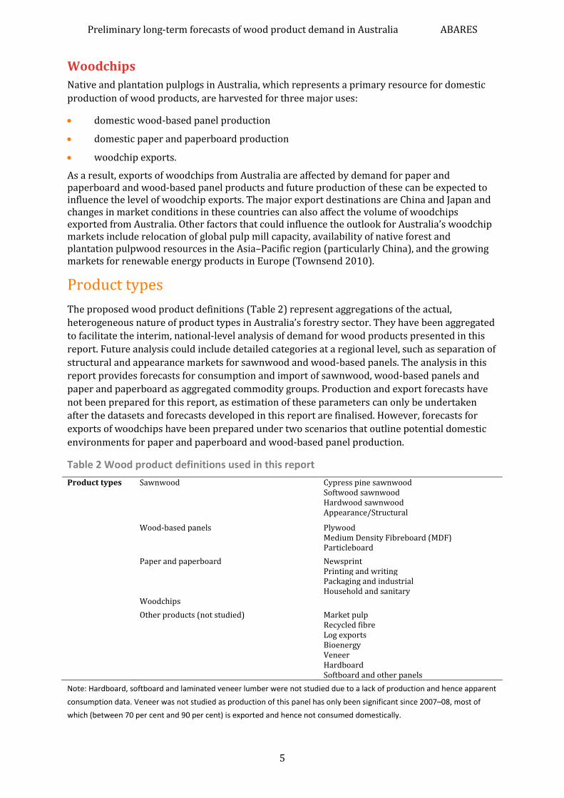
Product types
The proposed wood product definitions (Table 2) represent aggregations of the actual,
heterogeneous nature of product types in Australia’s forestry sector. They have been aggregated
to facilitate the interim, national-level analysis of demand for wood products presented in this
report. Future analysis could include detailed categories at a regional level, such as separation of
structural and appearance markets for sawnwood and wood-based panels. The analysis in this
report provides forecasts for consumption and import of sawnwood, wood-based panels and
paper and paperboard as aggregated commodity groups. Production and export forecasts have
not been prepared for this report, as estimation of these parameters can only be undertaken
after the datasets and forecasts developed in this report are finalised. However, forecasts for
exports of woodchips have been prepared under two scenarios that outline potential domestic
environments for paper and paperboard and wood-based panel production.
Table 2 Wood product definitions used in this report
Product types Sawnwood Cypress pine sawnwood Softwood sawnwood
Hardwood sawnwood Appearance/Structural
Wood-based panels Plywood Medium Density Fibreboard (MDF) Particleboard
Paper and paperboard Newsprint Printing and writing Packaging and industrial Household and sanitary Woodchips
Other products (not studied) Market pulp Recycled fibre Log exports Bioenergy Veneer Hardboard Softboard and other panels
Note: Hardboard, softboard and laminated veneer lumber were not studied due to a lack of production and hence apparent
consumption data. Veneer was not studied as production of this panel has only been significant since 2007–08, most of
which (between 70 per cent and 90 per cent) is exported and hence not consumed domestically.

Preliminary long-term forecasts of wood product demand in Australia ABARES
6
3 Key datasets The forecasting analysis presented in this report uses a number of additional assumptions
relating to resource, macroeconomic and demographic parameters. The key assumptions
employed in the analysis are in Table 3, and Appendix B provides a more detailed description of
the sources and methodology employed to derive these parameters.
Table 3 Assumptions used in business-as-usual scenario
Unit 2009–10 d 2019–20 2029–30 2039–40 2049–50 Domestic resources Hardwood plantation area ’000 ha 980 980 980 980 980 Softwood plantation area ’000 ha 1 025 1 025 1 025 1 025 1 025 Domestic markets Real GDP 2010A$b 1 284 1 719 2 111 2 526 2 961 Interest rate % 6.0 6.8 6.8 6.8 6.8 Population million 22.3 25.5 29.0 32.4 35.7 Real GDP per capita 2010A$ 57 576 67 513 72 707 77 914 82 843 Manufacturing output
(value added) a
Base 2010A$b 107.7 127.3 131.3 131.9 129.8 High 2010A$b – 133.7 137.8 138.5 136.3 Low 2010A$b – 121.0 124.7 125.3 123.3 Domestic housing market Household size People/
household 2.52 2.45 2.38 2.31 2.24
Share of multi-dwellings % 32 38 41 45 48 Value of renovations b Base 2010A$b 6.5 9.1 12.6 16.8 21.7 High 2010A$b – 9.5 13.3 17.7 22.8 Low 2010A$b – 8.6 12.0 16.0 20.7 Dwelling commencements c Total dwellings Base ’000 165.5 184.3 193.6 198.3 214.7 High ’000 – 193.6 203.3 208.2 225.4 Low ’000 – 175.1 183.9 188.4 203.9 Detached dwellings Base ’000 112.1 114.8 114.0 110.0 111.8 High ’000 – 120.6 119.7 115.5 117.4 Low ’000 – 109.1 108.3 104.5 106.2 Multi-dwellings Base ’000 53.4 69.5 79.6 88.3 102.9 High ’000 – 73.0 83.6 92.7 108.0 Low ’000 – 66.0 75.6 83.9 97.7 World markets Exchange rate US$/A$ 0.88 1.00 1.00 1.00 1.00
Note: a A +/- 5 per cent deviation from the baseline projection for manufacturing output (value added) is used to
demonstrate the sensitivity of consumption and import forecasts to variations in this variable. A 5 per cent deviation was
chosen arbitrarily to acknowledge potential errors and the uncertainty associated with ABARES projection for
manufacturing output. b Value of renovations is reported here in 2010 Australian dollars using the ABS housing CPI re-
based to 2009–10 dollars to allow for comparison with other market variables. Forecasting models apply the ABS housing
CPI based on 2003–04 dollars, as discussed in Appendix B. c The ‘high’ and ‘low’ estimates for dwelling commencements are
based on a +/- 5 per cent deviation from the baseline projection for total dwellings. A 5 per cent deviation was chosen by
examining the error margin for dwelling commencement projections in Love and colleagues (1999).This acknowledges the
potential errors and uncertainty associated with ABARES projections for total dwelling commencements. The detailed
methodology behind dwelling commencement projections used in this report is outlined in Appendix B. d 2009–10 is used
as the base year in this table based on currently available information for all variables and to facilitate comparisons
between macroeconomic variables.
Sources: Australian Government 2011; ABARES datasets

Preliminary long-term forecasts of wood product demand in Australia ABARES
7
Over the period to 2049–50, real GDP growth in Australia is assumed to average 2.1 per cent a
year based on projections made by the ABARES Global Trade and Environment Model (GTEM).
Annual growth in manufacturing output is assumed to be slower, at 0.5 per cent based on
ABARES baseline projections. Population growth is assumed to be 1.21 per cent based on
assumptions made by the Australian Treasury (Australian Government 2011). The implication of
these projections is that the real value of per capita GDP in Australia is estimated to reach
$82 843 by 2049–50 (in 2010 dollars) compared with $57 576 in 2009–10. Given the short-run
volatility of exchange rates, ABARES assumed a convergence to a long-term parity between
2011–12 and 2049–50. The detailed methodology behind these assumptions is discussed in
Appendix B.
Key variables for forecasting consumption of structural timber products are those relating to
housing sector activity in Australia. Based on historical trends, ABARES estimated the number of
new housing commencements to 2049–50, based on assumptions made for household sizes over
this period. The total number of dwelling commencements in Australia is forecast to increase
from around 157 430 dwellings in 2010–11 to around 214 600 dwellings in 2049–50. This
growth is driven by an increase in Australia’s population and a decrease in household size.
The share of multi-dwellings in total housing activity has also been forecast over the period to
2049–50. This share is assumed to increase from 38 per cent in 2010–11 to 48 per cent by
2049–50. This is based on historical trends seen in the urbanisation of Australia’s population,
and described further in Appendix B. Briefly, forecasts for the proportions of multi and detached
dwelling commencements, based on the State of Australian Cities 2010 report (Infrastructure
Australia 2010), suggest that much of the population growth to 2049–50 will occur in capital
cities. Consequently, as large cities grow to accommodate expanding populations, it is expected
that a higher proportion of multi-dwellings will be constructed. ABARES estimates that relative
to 2010–11 the number of multi-dwelling commencements in Australia will increase by 31.7 per
cent in 2029–30 and 70 per cent in 2049–50.
Based on historical trends in the real value of alterations and additions, the baseline estimate for
growth in the real value of renovation activity averages 3.1 per cent over the forecast period,
which is above the rate of housing or GDP growth (Appendix B). Hence, the real value of
renovations is forecast to nearly double by 2029–30 and increase by 235 per cent in 2049–50
relative to 2010–11.
Forecasts of pulplog availability
The forecasts of pulplog availability represent ABARES estimates based on previously compiled
publicly available datasets developed for Potential effects of climate change on forests and
forestry (ABARES 2012) and Australia’s Plantation Log Supply 2010–2054 (Gavran et al. 2012) as
well as anecdotal information from the industry. The detailed methodology underpinning the
pulplog availability forecasts presented in this section is discussed in both reports. The forecasts
are based on the assumption that harvested areas will be replanted with the same type of
plantation species. The forecasts do not take into account any future management decisions such
as plantations with low growth rates not being replanted and converted to another land use. As
information becomes available, the forecasts may be revised to reflect further changes.
Based on log harvest ratios in Appendix B, an estimate for the actual harvest of pulplogs was
derived. The results for selected periods are shown in Table 4.

Preliminary long-term forecasts of wood product demand in Australia ABARES
8
Table 4 Availability of pulplogs and harvest of pulplogs in Australia (annual average in ’000 m3), 2010–14, 2030–34 and 2045–49
Pulplog type 2010–14 2030–34 2045–49 Availability Harvest Availability Harvest Availability Harvest
Total native pulplogs 4 372 4 154 3 013 2 863 3 024 2 873 Hardwood plantation pulplogs 9 162 6 225 12 820 8 710 12 172 8 270 Softwood plantation pulplogs 5 555 4 999 6 035 5 432 5 992 5 393 Total pulplogs 19 090 15 379 21 869 17 005 21 188 16 536
Note: There is a range of views on the potential future plantation area and production over the forecast period. Some
anecdotal information from industry was incorporated in these forecasts.
Source: ABARES Datasets. Business-as-usual assumptions for pulplogs are based on the methodology outlined in ABARES
(2012) and Gavran and colleagues (2012).
This report does not examine the differences in native and plantation, and hardwood and
softwood pulplogs. Future research using the FORUM model could investigate the implications
for production and export forecasts on the basis of supply of particular resources and inputs for
different commodity groups.
The existing datasets project average annual availability of pulplogs in five-yearly periods
between 2010–14 and 2045–49. In this report, ABARES assumed the average annual availability
of pulplogs represents availability in the middle of each five-year period. For example, total
pulplog availability in 2011–12 and 2016–17 was assumed to be 19.1 million cubic metres and
21.2 million cubic metres based on estimates for 2010–14 and 2015–19 respectively (ABARES
estimates). A linear trend was then used to interpolate the availability in intervening years
between each midpoint. Based on log harvest ratios in Appendix B, actual harvest of pulplogs
was estimated for each year in the forecast period (Figure 1). For instance, total pulplog harvest
in 2011–12 and 2016–17 was estimated to be 15.4 million cubic metres and 16.7 million cubic
metres respectively.
Figure 1 Volume of logs harvested, historical 1991–11, forecasts 2012–50
Source: ABARES forecasts
0
2000
4000
6000
8000
10000
12000
14000
16000
18000
19
95
20
00
20
05
20
10
20
15
20
20
20
25
20
30
20
35
20
40
20
45
20
50
Vo
lum
e o
f lo
gs h
arve
ste
d (
'00
0 m
3)
Years
Pulplog harvest - historical Pulplog harvest - forecast

Preliminary long-term forecasts of wood product demand in Australia ABARES
9
4 Sawnwood forecasts Sawnwood consumption and imports are forecast to increase between 2011–12 and 2049–50.
Imports are estimated to grow marginally faster than consumption. As a result, the ratio of
imports to consumption is estimated to increase over the forecast period (Table 8). However,
the level of imports will also depend on other factors, particularly, domestic demand and supply.
It is difficult to predict the implications for domestic production and exports given the relatively
wide range presented by the 95 per cent confidence intervals over a long forecast time horizon.
Further research could examine an integrated framework through the FORUM model to estimate
future domestic production and exports.
Sawnwood consumption
Sawnwood consumption comprises hardwood and softwood sawnwood. ABARES modelled the
total quantity of sawnwood consumption for the period 2012 to 2050. Financial year historical
data (1978–2011) were used to develop an econometric model to estimate and test the
relationship between sawnwood consumption and commencements of multi-dwellings and
detached dwellings. The housing industry is a large user of structural sawnwood and represents
a domestic demand factor. The estimated model suggests that positive or negative changes in the
number of dwelling commencements have a corresponding effect on sawnwood consumption.
Sawnwood consumption over the past 30 years shows a marginal upward trend. Dwelling
commencements are typically a leading indicator of the economy and significant shocks to the
macro-economy (such as introduction of the goods and services tax in 2000 and the 2008 global
financial crisis) have also affected sawnwood consumption.
A range of macroeconomic variables including real GDP per capita and household income were
also considered. However, after accounting for outliers and cyclical components, the best fit for
the model used commencements of detached and multi-dwellings as the primary drivers of
consumption of sawnwood. Figure 2 shows how well the model fits actual data when
backcasting over the period 1978–2011. Actual sawnwood consumption during this period is
within the constructed 95 per cent confidence interval (which approximately represents two
standard errors above and below model estimates) and is followed closely by model estimates.
The model largely captures directional movements in actual data with minor departures from
the trend.
Details of the model structure and assumptions are in Appendixes A and B. Forecasts in Figure 3
and Table 5 show an increase in consumption of sawnwood between 2011–12 and 2049–50.
This increase is driven by the number of dwelling commencements which is forecast to increase
based on assumptions described in the data section and further discussed in Appendix B.
ABARES estimates that the number of total dwelling commencements will increase by 23 per
cent in 2029–30 and 36 per cent in 2049–50 relative to 2010–11. This has resulted in the
observed trend in sawnwood consumption forecasts (Figure 3, Table 5).
However, sawnwood consumption per capita is expected to decrease between 2029–30 and
2049–50 (Table 5). This is likely driven by concentration of population growth in large cities
resulting in a structural shift from detached dwellings to multi-dwellings which are estimated to
require less wood per dwelling constructed. This model is calibrated to primarily capture the
structural components of sawnwood consumption and examination of the demand factors
influencing appearance grade sawnwood may provide additional insights. Future research could
also seek to split sawnwood consumption into hardwood and softwood components.

Preliminary long-term forecasts of wood product demand in Australia ABARES
10
Figure 2 Sawnwood consumption model performance, actual 1978–2011
Source: ABARES models
Table 5 Summary of forecasts for modelling inputs and sawnwood consumption, 2010–14, 2030–34 and 2045–49
Unit 2010–14 2030–34 2045–49 Mean sawnwood consumption ’000 m3 4 991 6 014 6 374 Mean no. of detached dwelling commencements ’000 100.1 113.0 111.1 Mean no. of multi-dwelling commencements ’000 55.5 81.2 98.1 Mean sawnwood consumption per capita m3 0.220 0.202 0.183
Source: ABARES forecasts
0
1000
2000
3000
4000
5000
6000
7000
19
80
19
85
19
90
19
95
20
00
20
05
20
10
Co
nsu
mp
tio
n o
f sa
wn
wo
od
('0
00
m3
)
Years
Sawnwood Consumption (Actual)
Sawnwood Consumption (Model)

Preliminary long-term forecasts of wood product demand in Australia ABARES
11
Figure 3 Sawnwood consumption, actual 1978–2011, forecast 2012–50
Note: The confidence interval gives a range with 95 per cent certainty for the forecasts under business-as-usual
assumptions. This range is based on the standard errors of forecasts, determined by the modelled relationship between the
dependant variable and explanatory variables. Future shocks to explanatory variables and the modelled relationship are not
captured by this range.
Source: ABARES forecasts
Range and sensitivity of forecasts
The forecasts Love and colleagues made in 1999 were relatively conservative and forecast
consumption of sawnwood to average 4.2 million cubic metres in 2009–10 (compared with 5.4
million cubic metres actually consumed in 2009–10) and average 5.1 million cubic metres in the
five years to 2039–40 (compared with a forecast 6.2 million cubic metres consumed in 2039–40
in this report). Love and colleagues used a log model to forecast structural wood products
(which includes softwood and hardwood sawnwood, and panels) using detached and multi-
dwelling commencements, real GDP and structural wood consumption in the previous year as
explanatory variables. In this report a first difference log model was used, and accounting for
outliers and cyclical components, sawnwood consumption was regressed on detached and
multi-dwelling commencements.
The 95 per cent confidence interval provides a range for the forecasts under the assumptions
made for the business-as-usual scenario. However, the range provided by the 95 per cent
confidence interval limits the variability of exogenous parameters and does not allow for
potential future errors in the assumptions. Sawnwood consumption is estimated to increase
from 5.0 million cubic metres in 2010–11 to 6.0 million cubic metres in 2029–30 and 6.5 million
cubic metres in 2049–50 (Table 6). The 95 per cent confidence interval suggests that
0
1000
2000
3000
4000
5000
6000
7000
8000
9000
19
80
19
85
19
90
19
95
20
00
20
05
20
10
20
15
20
20
20
25
20
30
20
35
20
40
20
45
20
50
Co
nsu
mp
tio
n o
f sa
wn
wo
od
('0
00
m3
)
Years
95% Confidence Interval
Sawnwood Consumption (Forecast)
Sawnwood Consumption (Actual)

Preliminary long-term forecasts of wood product demand in Australia ABARES
12
consumption is likely to be between 5.1 million and 6.8 million cubic metres in 2029–30 and
between 5.5 million and 7.4 million cubic metres in 2049–50.
Table 6 Forecast summary for sawnwood consumption
Year Estimate ’000 m3
95 per cent confidence interval ’000 m3
2010–11 a 5 047 – 2029–30 5 984 ± 831 2049–50 6 475 ± 924
Note: a Actual as at May 2012 and may have been revised since.
Source: ABARES forecasts
The model results (outlined in Appendix A) suggest a positive coefficient for multi-dwelling and
detached dwelling commencements (explanatory variables). Therefore a positive change in the
explanatory variables results in a corresponding positive change in the quantity of sawnwood
consumption. Specifically, a 1 per cent increase in detached or multi-dwelling commencements
is estimated to result in a 0.12 per cent and 0.32 per cent increase in sawnwood consumption,
respectively.
The volume of sawnwood consumption will change if the number of dwelling commencements
deviates from the baseline case to the ‘high’ and ‘low’ estimates described in Table 3. Table 7
shows the sensitivity of the forecast for sawnwood consumption to changes in key demand
variables—detached and multi-dwelling commencements.
Table 7 Sensitivity of sawnwood consumption forecasts
Unit 2010–11 2029–30 2049–50 Sensitivity to changes in detached dwelling commencements a Detached dwelling commencements Base ’000 97.1 114 111.8 High ’000 – 119.7 117.4 Low ’000 – 108.3 106.2 Sawnwood consumption Base ’000 m3 5 047 c 5 984 6 475 High ’000 m3 – 6 021 6 515 Low ’000 m3 – 5 947 6 435 Sensitivity to changes in multi-dwelling commencements a Multi-dwelling commencements Base ’000 60.4 79.6 102.9 High ’000 – 83.6 108.0 Low ’000 – 75.6 97.7 Sawnwood consumption Base ’000 m3 5 047 c 5 984 6 475 High ’000 m3 – 6 079 6 578 Low ’000 m3 – 5 889 6 372
Note: The ‘high’ and ‘low’ estimates for total dwelling commencements are based on a +/- 5 per cent deviation from the
baseline projection for total dwellings. A 5 per cent deviation was chosen by examining the error margin for dwelling
commencement projections in Love and colleagues (1999). The detailed methodology behind ‘high’ and ‘low’ estimates for
detached and multi-dwelling commencements is outlined in Appendix B. a Changes in sawnwood consumption are based
on estimated model coefficients multiplied by the size of the percentage change in detached and multi-dwelling
commencements. b Actual as at May 2012 and may have been revised since.
If detached dwelling commencements deviate from the baseline estimate to the ‘high’ estimate
(from around 111 800 to around 117 400), sawnwood consumption increases marginally from
around 6.48 million cubic metres to 6.51 million cubic metres (Table 7). That is, all other
variables being equal, in 2049–50 for a 5 per cent increase in detached dwelling
commencements, sawnwood consumption increases by 0.62 per cent.

Preliminary long-term forecasts of wood product demand in Australia ABARES
13
The forecast for sawnwood consumption is more sensitive to changes in multi-dwelling
commencements. If multi-dwelling commencements deviate from the baseline estimate to the
‘high’ estimate (from around 102 900 to around 108 000), sawnwood consumption increases
from around 6.48 million cubic metres to 6.57 million cubic metres (Table 7). That is, all other
variables being equal, for a 5 per cent increase in multi-dwelling commencements, sawnwood
consumption increases by 1.59 per cent.
Sawnwood imports
Sawnwood imports to Australia comprise hardwood and softwood sawnwood. ABARES
modelled the total quantity of sawnwood imports for the period 2011–12 to 2049–50. Financial
year historical data (1988–89 to 2010–11) were used to develop an econometric model to
estimate and test the relationship between sawnwood imports and the number of multi-
dwellings commenced together with the Australian to US dollar exchange rate. Multi-dwelling
commencements act as a domestic demand indicator affecting the level of sawnwood imports
particularly for structural wood and furniture.
The Australian to US dollar exchange rate is a measure of the purchasing power of the Australian
dollar. An appreciation in the Australian dollar generally results in cheaper imports. As a result,
it is estimated that positive or negative changes in both explanatory variables will have a
corresponding positive or negative effect on sawnwood imports. Figure 4 shows the accuracy of
the constructed model when backcasting over the period 1989–2011. Actual sawnwood import
during this period is within the constructed 95 per cent confidence interval (which
approximately represents two standard errors above and below model estimates) and is
followed closely by model estimates. The model appears to capture almost all directional
movements in actual data and although the approximations are sometimes exaggerated, actual
data remains within the 95 per cent confidence interval.
The volume of imports will also depend on domestic demand and supply conditions. Although
the model includes a demand indicator (multi-dwelling commencements), domestic
consumption was not included as an explanatory variable given the definition of apparent
consumption. Future research could examine domestic production and exports through the
ABARES FORUM model and could seek to integrate consumption and import forecasts to present
a complete outlook. Globally, changes in the US housing market and growth in Chinese demand
for softwood sawnwood may influence sawnwood trade. The United States is the world’s largest
importer of softwood sawnwood and China looks to be increasing its share in global sawnwood
markets (Burke & Townsend 2011).
Details of the model structure and assumptions are presented in Appendix A and Appendix B.
Despite a fall in the volume of imports over the decade between 1990 and 2000, imports of
sawnwood increased and are forecast to continue increasing between 2011–12 and 2049–50
(Figure 5, Table 8). The increase in sawnwood imports is driven by an increase in multi-dwelling
commencements (see Key datasets, Appendix B). Exchange rates are estimated to have a
relatively smaller influence on forecasts for sawnwood imports.

Preliminary long-term forecasts of wood product demand in Australia ABARES
14
Figure 4 Sawnwood imports model performance, actual 1990–2011
Source: ABARES models
The observed trend in sawnwood import forecasts is driven by the increased growth in multi-
dwelling commencements. The forecast mean sawnwood imports per capita is also estimated to
increase marginally before levelling off (Table 8). This corresponds with a faster growth in
imports than in population initially as suggested by strong growth in demand indicators such as
the number of multi-dwelling commencements. Between 2029–30 and 2049–50 this growth is
expected to stabilise matching the growth in population. The model for sawnwood imports
places a higher weight than the model for sawnwood consumption on the number of multi-
dwelling commencements. The number of multi-dwelling commencements is a primary
explanatory variable in both models and is projected to account for most of the increase in total
dwelling commencements. Thus, the forecast mean proportion of sawnwood imports to
consumption is estimated to increase.
Table 8 Summary of forecasts for modelling inputs and sawnwood imports (annual average), 2010–14, 2030–34 and 2045–49
Unit 2010–14 2030–34 2045–49 Mean sawnwood imports ’000 m3 830 1 242 1 430 Mean no. of multi-dwelling commencements ’000 55.5 81.2 98.1 Mean value of the US dollar against the Australian dollar US$/A$ 0.995 1.000 1.000 Mean sawnwood imports per capita m3 0.037 0.042 0.041 Mean proportion of sawnwood imports to consumption % 16.6 20.7 22.4
Source: ABARES forecasts
0
200
400
600
800
1000
1200
1400
1600
19
90
19
95
20
00
20
05
20
10
Imp
ort
s o
f sa
wn
wo
od
('0
00
m3
)
Years
Sawnwood Imports (Actual)
Sawnwood Imports (Model)

Preliminary long-term forecasts of wood product demand in Australia ABARES
15
Figure 5 Sawnwood imports, actual 1990–2011, forecast 2012–50
Note: The confidence interval gives a range with 95 per cent certainty for the forecasts under the business-as-usual
assumptions. This range is based on the standard errors of forecasts, determined by the modelled relationship between the
dependant variable and explanatory variables. Future shocks to explanatory variables and the modelled relationship are not
captured by this range.
Source: ABARES forecasts
Range of forecasts
Sawnwood imports are forecast to increase by around 75 per cent over the 40-year forecast
period (Table 9), from around 0.8 million cubic metres in 2010–11 to 1.2 million cubic metres in
2029–30 and 1.5 million cubic metres in 2049–50. The 95 per cent confidence interval provides
a range for the forecasts under the assumptions made for the business-as-usual scenario. Here
sawnwood imports are likely to be between 0.9 million and 1.6 million cubic metres in 2029–30
and between 1 million and 1.9 million cubic metres in 2049–50.
Table 9 Forecast summary for sawnwood imports
Year Estimate ’000 m3
95 per cent confidence interval ’000 m3
2010–11 a 846 – 2029–30 1 225 ± 357 2049–50 1 481 ± 438
Note: a Actual as at May 2012 and may have been revised since.
Source: ABARES forecasts
0
500
1000
1500
2000
2500
19
90
19
95
20
00
20
05
20
10
20
15
20
20
20
25
20
30
20
35
20
40
20
45
20
50
Imp
ort
s o
f sa
wn
wo
od
('0
00
m3
)
Years
95% Confidence Interval
Sawnwood Imports (Forecast)
Sawnwood Imports (Actual)

Preliminary long-term forecasts of wood product demand in Australia ABARES
16
5 Wood-based panel forecasts Wood-based panel consumption and imports are forecast to increase between 2011–12 and
2049–50. Consumption is forecast to grow at a faster rate than imports. Therefore, the ratio of
imports to consumption is forecast to decrease over the analysis period (Table 13).
Consumption of wood-based panels is closely linked to the number of multi-dwelling
commencements. As well, imports may be affected by domestic supply factors. It is worth noting
that imports of wood-based panels have historically been relatively small compared with other
wood product imports.
Wood-based panel consumption
Wood-based panel consumption estimated in this report consists of plywood, particleboard and
medium density fibreboard. These panels are largely used for structural purposes in building
activities. Given the wide variety of uses for wood-based panels, the models were calibrated to
focus on structural timber uses. Hardboard, softboard and laminated veneer lumber were not
studied due to a lack of sufficient production and hence apparent consumption data. Veneer was
not included as production of this panel has only been significant since 2007–08, most of which
(between 70 and 90 per cent) is exported and hence not consumed domestically.
ABARES modelled forecasts for the total quantity of wood-based panel consumption for the
period 2012 to 2049–50. Financial year historical data (1978–2011) were used to develop an
econometric model to estimate and test the relationship between wood-based panel
consumption and multi-dwelling commencements together with the real value of approved
alterations and additions (or renovations) to existing houses. The housing industry is a large
user of wood-based panels—primarily in wall, roof and floor sheathing—but also in cabinets,
mouldings and doors. Wood-based panels are also used in furniture construction.
Analysing wood-based panel consumption shows the need to account for outliers and a cyclical
trend in the data. A number of macroeconomic variables including real GDP per capita and
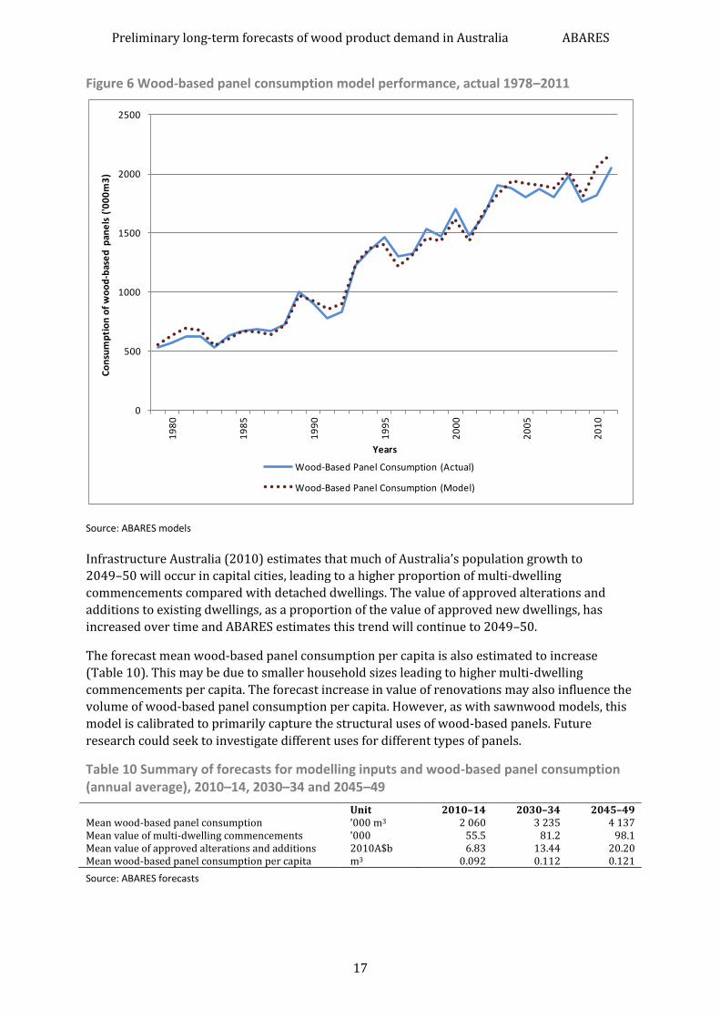
household income were also considered. Figure 6 shows how well the model fits actual data
when backcasting over the period 1978–2011. Actual wood-based panel consumption during
this period is within the constructed 95 per cent confidence interval (which approximately
represents two standard errors above and below model estimates) and is followed closely by
model estimates. In particular, the model accurately captures directional movements in actual
data in the 1980s and 1990s with minor departures from the trend in the 2000s.
Details of the model structure and assumptions are presented in Appendix A and Appendix B.
The forecasts in Figure 7 and Table 11 show an increase in consumption of wood-based panels
between 2011–12 and 2049–50. This increase is driven by the number of multi-dwelling
commencements and the real value of renovations, which are forecast to increase, based on
assumptions in Appendix B. ABARES estimates the number of multi-dwelling commencements
to rise by 32 per cent in 2029–30 and 70 per cent in 2049–50 relative to 2010–11. Similarly, the
real value of renovations is estimated to increase 95 per cent by 2029–30 and 235 per cent by
2049–50 relative to 2010–11. This has resulted in the observed trend in wood-based panel
consumption forecasts (Figure 7, Table 11).
Preliminary long-term forecasts of wood product demand in Australia ABARES
17
Figure 6 Wood-based panel consumption model performance, actual 1978–2011
Source: ABARES models
Infrastructure Australia (2010) estimates that much of Australia’s population growth to
2049–50 will occur in capital cities, leading to a higher proportion of multi-dwelling
commencements compared with detached dwellings. The value of approved alterations and
additions to existing dwellings, as a proportion of the value of approved new dwellings, has
increased over time and ABARES estimates this trend will continue to 2049–50.
The forecast mean wood-based panel consumption per capita is also estimated to increase
(Table 10). This may be due to smaller household sizes leading to higher multi-dwelling
commencements per capita. The forecast increase in value of renovations may also influence the
volume of wood-based panel consumption per capita. However, as with sawnwood models, this
model is calibrated to primarily capture the structural uses of wood-based panels. Future
research could seek to investigate different uses for different types of panels.
Table 10 Summary of forecasts for modelling inputs and wood-based panel consumption (annual average), 2010–14, 2030–34 and 2045–49
Unit 2010–14 2030–34 2045–49 Mean wood-based panel consumption ’000 m3 2 060 3 235 4 137 Mean value of multi-dwelling commencements ’000 55.5 81.2 98.1 Mean value of approved alterations and additions 2010A$b 6.83 13.44 20.20 Mean wood-based panel consumption per capita m3 0.092 0.112 0.121
Source: ABARES forecasts
0
500
1000
1500
2000
2500
19
80
19
85
19
90
19
95
20
00
20
05
20
10
Co
nsu
mp
tio
n o
f w
oo
d-b
ase
d p
ane
ls (
'00
0m
3)
Years
Wood-Based Panel Consumption (Actual)
Wood-Based Panel Consumption (Model)

Preliminary long-term forecasts of wood product demand in Australia ABARES
18
Figure 7 Wood-based panel consumption, actual 1978–2011, forecast 2012–50
Note: The confidence interval gives a range with 95 per cent certainty for the forecasts under the business-as-usual
assumptions. This range is based on the standard errors of forecasts, determined by the modelled relationship between the
dependant variable and explanatory variables. Future shocks to explanatory variables and the modelled relationship are not
captured by this range.
Source: ABARES forecasts
Range of forecasts
Love and colleagues (1999) used a log model to forecast consumption of total structural wood
products. Consumption of wood-based panels was forecast to average 1.5 million cubic metres
in the five years to 2009–10 (compared with 1.8 million cubic metres actually consumed in
2009–10) and average 1.8 million cubic metres in the five years to 2039–40 (compared with a
forecast 3.7 million cubic metres consumed in 2039–40 in this report). Addressing one of the
challenges Love and colleagues faced in 1999, consumption and trade of sawnwood and wood-
based panels were forecast separately in this report. Analysis shows that consumption of
sawnwood and of wood-based panels do not necessarily have similar trends over time.
The 95 per cent confidence interval provides a range for the forecasts under the assumptions
made for the business-as-usual scenario. However, the range provided by the 95 per cent
confidence interval limits the variability of exogenous parameters and does not allow for
potential future errors in the assumptions. ABARES forecasts that consumption of wood-based
panels will increase from 2.0 million cubic metres in 2010–11 to 3.1 million cubic metres in
2029–30 and 4.3 million cubic metres in 2049–50 (Table 11). The 95 per cent confidence
interval provides a range for these forecasts and suggests wood-based panel consumption will
be between 2.6 million and 3.6 million cubic metres in 2029–30 and between 3.6 million and
5.1 million cubic metres in 2049–50.
0
1000
2000
3000
4000
5000
6000
19
80
19
85
19
90
19
95
20
00
20
05
20
10
20
15
20
20
20
25
20
30
20
35
20
40
20
45
20
50
Co
nsu
mp
tio
n o
f w
oo
d-b
ase
d p
ane
ls (
'00
0m
3)
Years
95% Confidence Interval
Wood-Based Panel Consumption (Forecast)
Wood-Based Panel Consumption (Actual)

Preliminary long-term forecasts of wood product demand in Australia ABARES
19
Table 11 Forecast summary for wood-based panel consumption
Year Estimate ’000 m3
95 per cent confidence interval ’000 m3
2010–11 2 048 a –
2029–30 3 126 ± 497
2049–50 4 341 ± 715
Note: a Actual as at May 2012 and may have been revised since.
Source: ABARES forecasts
The model results (outlined in Appendix A) suggest a positive coefficient for both multi-dwelling
commencements and the value of renovations (explanatory variables). Therefore a positive
change in the explanatory variables results in a corresponding positive change in the quantity of
wood-based panel consumption. Specifically, a 1 per cent increase in multi-dwelling
commencements results in a 0.26 per cent increase in the rate of growth in wood-based panel
consumption. Similarly, a 1 per cent increase in the value of renovations results in a 0.48 per
cent increase in wood-based panel consumption.
ABARES tested the sensitivity of the forecast for wood-based panel consumption for a deviation
in the number of multi-dwelling commencements from the baseline case to the ‘high’ and ‘low’
estimates and changes in the value of renovations (Table 12).
Table 12 Sensitivity of wood-based panel consumption forecasts
Unit 2010–11 2029–30 2049–50 Sensitivity to changes in value of renovations a Value of renovations Base 2010A$b 6.7 12.6 21.7 High 2010A$b – 13.3 22.8 Low 2010A$b – 12.0 20.7 Wood-based panel consumption Base ’000 m3 2 048 b 3 126 4 341 High ’000 m3 – 3 201 4 445 Low ’000 m3 – 3 051 4 236 Sensitivity to changes in multi-dwelling commencements a Multi-dwelling commencements Base ’000 60.4 79.6 102.9 High ’000 – 83.6 108.0 Low ’000 – 75.6 97.7 Wood-based panel consumption Base ’000 m3 2 048 b 3 126 4 341 High ’000 m3 – 3 167 4 398 Low ’000 m3 – 3 085 4 283
Note: The ‘high’ and ‘low’ estimates for total dwelling commencements are based on a +/- 5 per cent deviation from the
baseline projection for total dwellings. A 5 per cent deviation was chosen by examining the error margin for dwelling
commencement projections in Love and colleagues (1999). The detailed methodology behind ‘high’ and ‘low’ estimates for
detached and multi-dwelling commencements is outlined in Appendix B. a Changes in wood-based panel consumption are
based on estimated model coefficients multiplied by the size of the percentage change in value of renovations and multi-
dwelling commencements. b Actual as at May 2012 and may have been revised since.
The forecast for wood-based panel consumption is more sensitive to changes in the value of
renovations. If value of renovations deviate from the baseline estimate and increases by 5 per
cent in 2049–50 (from around $21.7 billion to around $22.8 billion), wood-based panel
consumption increases from around 4.34 million cubic metres to 4.44 million cubic metres
(Table 12). That is, all other variables being equal, in 2049–50 for a 5 per cent increase in value
of renovations, wood-based panel consumption increases by 2.41 per cent.

Preliminary long-term forecasts of wood product demand in Australia ABARES
20
If multi-dwelling commencements deviate from the baseline estimate to the ‘high’ estimate
(from around 102 900 to around 108 000), wood-based panel consumption increases from
around 4.34 million cubic metres to 4.40 million cubic metres (Table 12). That is, all other
variables being equal, for a 5 per cent increase in multi-dwelling commencements, wood-based
panel consumption increases by 1.32 per cent.
Wood-based panel imports
Wood-based panel imports consist of plywood, particleboard and medium density fibreboard.
ABARES modelled forecasts for the total quantity of wood-based panel imports for the period
2012 to 2050. Financial year historical data (1989–2011) were used to develop an econometric
model to estimate and test the relationship between wood-based panel imports and multi-
dwellings commenced. Figure 8 shows how well the model fits actual data when backcasting
over the period 1989–2011. Actual wood-based panel imports during this period are within the
constructed 95 per cent confidence interval (which approximately represents two standard
errors above and below model estimates) and is followed closely by model estimates. The model
largely imitates the trend in actual data although there is evidence of increased variation in later
years which is expected given the size of the sample and small volumes of wood-based panel
imports. Rigorous testing shows that the model is stable and provides accurate forecasts under
the assumptions made for the business-as-usual scenario.
Compared with other wood product imports, the volume of wood-based panels imported has
been relatively small historically. However, domestic economic conditions and factors affecting
the domestic supply and demand for panels will affect the volume of imports. Some international
effects may also be captured through the Australian to US dollar exchange rate. Future research
could investigate major international markets for panels and their influence on Australian trade.
Details of the model structure and assumptions are presented in Appendix A and Appendix B.
The forecasts (Figure 9, Table 13) show an increase in imports of wood-based panels between
2011–12 and 2049–50 driven by an increase in multi-dwelling commencements. The model
suggests that positive or negative changes in multi-dwelling commencements will have a
corresponding positive or negative effect on wood-based panel imports. The number of multi-
dwelling commencements is forecast to increase based on assumptions presented in
Appendix B. This has led to the observed trend in wood-based panel import forecasts (Figure 9,
Table 13).
The forecast mean quantity of wood-based panel imports per capita between 2011–12 and
2049–50, is estimated to remain stable (Table 13). This reflects a growth in wood-based panel
imports that roughly matches growth in population over the forecast period. The forecast mean
proportion of wood-based panel imports to consumption is estimated to decrease, reflecting
higher growth in consumption compared with growth in imports under the business-as-usual
assumptions.

Preliminary long-term forecasts of wood product demand in Australia ABARES
21
Figure 8 Wood-based panel imports model performance, actual 1989–2011
Source: ABARES models
Table 13 Summary of forecasts for modelling inputs and wood-based panel imports (annual average), 2010–14, 2030–34 and 2045–49
Unit 2010–14 2030–34 2045–49 Mean wood-based panel imports ’000 m3 370 466 524 Mean multi-dwellings commencements ’000 55.5 81.2 98.1 Mean panel imports per capita m3 0.016 0.016 0.015 Mean proportion of panel imports to consumption % 18.0 14.4 12.7
Source: ABARES forecasts
0
50
100
150
200
250
300
350
400
450
19
90
19
95
20
00
20
05
20
10
Imp
ort
s o
f w
oo
d-b
ase
d p
ane
ls (
'00
0m
3)
Years
Wood-Based Panel Imports (Actual)
Wood-Based Panel Imports (Model)

Preliminary long-term forecasts of wood product demand in Australia ABARES
22
Figure 9 Wood-based panel imports, actual 1989–2011, forecast 2012–50
Note: The confidence interval gives a range with 95 per cent certainty for the forecasts under the business-as-usual
assumptions. This range is based on the standard errors of forecasts, determined by the modelled relationship between the
dependant variable and explanatory variables. Future shocks to explanatory variables and the modelled relationship are not
captured by this range.
Source: ABARES forecasts
Range of forecasts
ABARES forecasts a modest increase in wood-based panel imports over the period to 2049–50
(Table 14). Imports are estimated to increase from around 407 000 cubic metres in 2010–11 to
460 000 cubic metres in 2029–30 and 539 000 cubic metres in 2049–50. The 95 per cent
confidence interval provides a range for the forecasts under the assumptions made for the
business-as-usual scenario and suggests that imports will be between 300 000 cubic metres and
621 000 cubic metres in 2029–30 and between 345 000 cubic metres and 733 000 cubic metres
in 2049–50.
Table 14 Forecast summary for wood-based panel imports
Year Estimate ’000 m3
95 per cent confidence interval ’000 m3
2010–11 407 a – 2029–30 460 ± 161 2049–50 539 ± 194
Note: a Actual as at May 2012 and may have been revised since.
Source: ABARES forecasts
0
100
200
300
400
500
600
700
800
19
90
19
95
20
00
20
05
20
10
20
15
20
20
20
25
20
30
20
35
20
40
20
45
20
50
Imp
ort
s o
f w
oo
d-b
ase
d p
ane
ls (
'00
0m
3)
Years
95% Confidence Interval
Wood-Based Panel Imports (Forecast)
Wood-Based Panel Imports (Actual)

Preliminary long-term forecasts of wood product demand in Australia ABARES
23
6 Paper and paperboard forecasts Consumption and imports of paper and paperboard are forecast to increase between 2011–12
and 2049–50. As consumption is forecast to grow at a slower rate than imports, the ratio of
imports to consumption is expected to increase (Table 18). This is largely due to assumptions
made to forecast value added by the manufacturing sector. ABARES estimates that the
contribution of manufacturing to real GDP decreases over the forecast period. In this report,
value added by manufacturing sector and real GDP per capita are the primary explanatory
variables for forecasting consumption and imports of paper and paperboard products. Imports
may additionally be affected by domestic processing capacity and supply, and international
market conditions as indicated by world prices.
Paper and paperboard consumption
Paper and paperboard consumption comprises consumption of newsprint, household and
sanitary paper, packaging and industrial paper and printing and writing paper. ABARES
modelled forecasts for the total quantity of paper and paperboard consumption for the period
2012 to 2050. Financial year historical data (1983–2011) were used to develop an econometric
model to estimate and test the relationship between paper and paperboard consumption and
value added by manufacturing (chain volume measure). The manufacturing sector is a large user
of packaging and industrial paper and printing and writing paper and represents a domestic
demand factor. Consumption of these two grades of paper comprised 78 per cent of total paper
and paperboard consumption in Australia. It is estimated that positive or negative changes in the
value of manufacturing output have a corresponding effect on aggregate paper and paperboard
consumption.
It is difficult to estimate aggregate consumption because paper and paperboard products have a
wide range of end users (Edquist & Morris 1986). For example, while changes in the
manufacturing sector are unlikely to influence consumption or trade of newsprint and
household and sanitary paper products, they could be affected by changes in consumer income.
Ideally, models for forecasting paper consumption would consider the different grades of paper
separately and this may be examined in future research and analysis. Nevertheless, given that
packaging and industrial, and printing and writing paper, account for a significant proportion of
apparent consumption (78 per cent in 2010–11), the model presented in this report uses the
value added by the manufacturing sector as the primary explanatory variable. Figure 10 shows
how well the model fits actual data when backcasting over the period 1983–2011.
Actual paper and paperboard consumption during this period is within the constructed 95 per
cent confidence interval (which approximately represents two standard errors above and below
model estimates) and is followed closely by model estimates. The model largely captures
directional movements in actual data with minor departures from the trend. Rigorous testing
shows the model to be stable and accurate when forecasting under assumptions made for the
business-as-usual scenario.

Preliminary long-term forecasts of wood product demand in Australia ABARES
24
Figure 10 Paper and paperboard consumption model performance, actual 1983–2011
Source: ABARES models
Given that value added by manufacturing output is forecast to increase out to 2029–30 before
levelling off and declining marginally thereafter (Appendix B), paper and paperboard
consumption is forecast to increase between 2011–12 and 2049–50 (Figure 11, Table 16). This
is primarily due to the model structure (Appendix A) that shows a significant relationship for
manufacturing value added but also includes a constant term to capture the historical time trend
in aggregate paper consumption. This constant is necessary as it captures some of the variation
in newsprint and household grades of paper, thereby allowing use of manufacturing output to
explain consumption of packaging and printing grades of paper. The historical time trend
captured by this constant contributes to the trend in the forecast for aggregate paper and
paperboard consumption and is moderated by the primary explanatory variable—value added
by manufacturing output. Thus in later years, the decrease in manufacturing reduces paper and
paperboard consumption below the historical time trend. As real GDP is forecast to have stable
growth over this period, ABARES implicitly assumes that the value added by the manufacturing
sector to real GDP decreases. Details of the model structure and assumptions are presented in
Appendix A and Appendix B, respectively.
The mean quantity of paper and paperboard consumption is forecast to increase (Table 15)
driven by the increase in value added by the manufacturing sector. There is a marginal rise
forecast in consumption per capita. Between 2010–14 and 2030–34 consumption per capita is
expected to increase but will level off between 2030–34 and 2045–49 as manufacturing value
added also levels off. As the manufacturing sector is the major driver here, this forecast implies
that growth in consumption of packaging and industrial paper and printing and writing paper
0
1
2
3
4
5
19
85
19
90
19
95
20
00
20
05
20
10
Co
nsu
mp
tio
n o
f p
ape
r an
d p
ape
rbo
ard
(m
t)
Years
Paper and Paperboard Consumption (Actual)
Paper and Paperboard Consumption (Model)
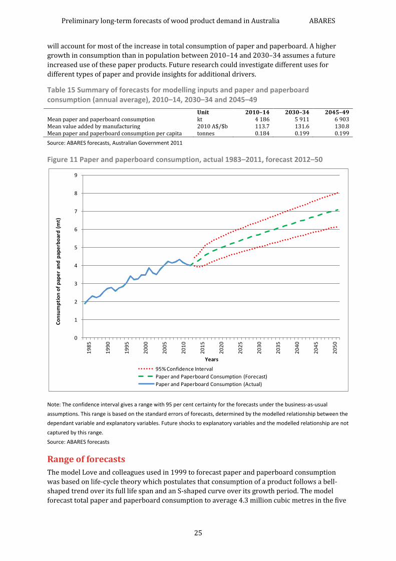
Preliminary long-term forecasts of wood product demand in Australia ABARES
25
will account for most of the increase in total consumption of paper and paperboard. A higher
growth in consumption than in population between 2010–14 and 2030–34 assumes a future
increased use of these paper products. Future research could investigate different uses for
different types of paper and provide insights for additional drivers.
Table 15 Summary of forecasts for modelling inputs and paper and paperboard consumption (annual average), 2010–14, 2030–34 and 2045–49
Unit 2010–14 2030–34 2045–49 Mean paper and paperboard consumption kt 4 186 5 911 6 903 Mean value added by manufacturing 2010 A$/$b 113.7 131.6 130.8 Mean paper and paperboard consumption per capita tonnes 0.184 0.199 0.199
Source: ABARES forecasts, Australian Government 2011
Figure 11 Paper and paperboard consumption, actual 1983–2011, forecast 2012–50
Note: The confidence interval gives a range with 95 per cent certainty for the forecasts under the business-as-usual
assumptions. This range is based on the standard errors of forecasts, determined by the modelled relationship between the
dependant variable and explanatory variables. Future shocks to explanatory variables and the modelled relationship are not
captured by this range.
Source: ABARES forecasts
Range of forecasts
The model Love and colleagues used in 1999 to forecast paper and paperboard consumption
was based on life-cycle theory which postulates that consumption of a product follows a bell-
shaped trend over its full life span and an S-shaped curve over its growth period. The model
forecast total paper and paperboard consumption to average 4.3 million cubic metres in the five
0
1
2
3
4
5
6
7
8
9
19
85
19
90
19
95
20
00
20
05
20
10
20
15
20
20
20
25
20
30
20
35
20
40
20
45
20
50
Co
nsu
mp
tio
n o
f p
ape
r an
d p
ape
rbo
ard
(m
t)
Years
95% Confidence Interval
Paper and Paperboard Consumption (Forecast)
Paper and Paperboard Consumption (Actual)

Preliminary long-term forecasts of wood product demand in Australia ABARES
26
years to 2009–10 (compared with the 4 million cubic metres actually consumed in 2009–10)
and average 6 million cubic metres in the five years to 2039–40 (compared with a forecast
5.9 million cubic metres consumed in 2040 in this report). The life-cycle method is not without
challenges, particularly the need to assume a discrete stage in the life cycle for each product.
Hence the approach used in this report is to account for business cycle components and estimate
the relationship between likely demand indicators and consumption.
The 95 per cent confidence interval provides a range for the forecasts under the assumptions
made for the business-as-usual scenario. However, the range provided by the 95 per cent
confidence interval limits the variability of exogenous parameters and does not allow for
potential future errors in the assumptions. Forecasts show that paper and paperboard
consumption will increase from 4 million tonnes in 2010–11 to 5.8 million tonnes in 2029–30
and 7.1 million tonnes in 2049–50 (Table 16). The 95 per cent confidence interval provides a
range for these forecasts and suggests that paper and paperboard consumption will be between
5.1 million tonnes and 6.5 million tonnes in 2029–30 and between 6.2 million tonnes and
8 million tonnes in 2049–50.
Table 16 Forecast summary for paper and paperboard consumption
Year Estimate ’000 tonnes
95 per cent confidence interval ’000 tonnes
2010–11 4 012 a – 2029–30 5 774 ± 715 2049–50 7 083 ± 932
Note: a Actual as at May 2012 and may have been revised since.
Source: ABARES forecasts
The model results (outlined in Appendix A) suggest a positive coefficient for value added by
manufacturing output (explanatory variable). Therefore a positive change in the explanatory
variable results in a corresponding positive change in the quantity of wood-based panel
consumption. Specifically, a 1 per cent increase in manufacturing output results in a 0.82 per
cent increase in paper and paperboard consumption. ABARES tested the sensitivity of the
forecast for paper and paperboard consumption for changes in manufacturing (Table 12).
Table 17 Sensitivity of paper and paperboard consumption forecasts
Unit 2010–11 2029–30 2049–50 Sensitivity to changes in value added by the manufacturing output a Manufacturing output (value added) Base 2010A$b 107.8 131.3 129.8 High 2010A$b – 137.8 136.3 Low 2010A$b – 124.7 123.3 Paper and paperboard consumption Base ’000 tonnes 4 012 b 5 774 7 083 High ’000 tonnes – 6 011 7 374 Low ’000 tonnes – 5 537 6 793
Note: A +/- 5 per cent deviation from the baseline projection for manufacturing output (value added) is used to
demonstrate the sensitivity of consumption and import forecasts to variations in this variable. A 5 per cent deviation was
chosen arbitrarily to acknowledge potential errors and the uncertainty associated with ABARES projection for
manufacturing output. a Changes in paper and paperboard consumption are based on the estimated model coefficient
multiplied by the size of the percentage change in manufacturing. b Actual as at May 2012 and may have been revised
since.
The forecast for paper and paperboard consumption is sensitive to changes in the value added
by manufacturing output. It is important to remember that changes in manufacturing are more
likely to affect consumption of packaging and industrial and printing and writing grades of

Preliminary long-term forecasts of wood product demand in Australia ABARES
27
paper. If value added by manufacturing increases by 5 per cent in 2049–50 (from around
$129.8 billion to around $136.3 billion), paper and paperboard consumption increases from
around 7.08 million cubic metres to 7.37 million cubic metres (Table 17). That is, all other
variables being equal, for a 5 per cent increase in manufacturing, paper and paperboard
consumption increases by 4.10 per cent.
Paper and paperboard imports
Paper and paperboard imports comprise newsprint, household and sanitary paper, packaging
and industrial paper and printing and writing paper. ABARES modelled forecasts for the total
quantity of paper and paperboard imports for the period 2011–50 using financial year historical
data (1983–2010). An econometric model was developed to test the relationship between paper
and paperboard imports and the value of GDP product per capita. This variable was used to
estimate the relationship between domestic macroeconomic activity and paper and paperboard
imports, in lieu of a direct demand factor. Hence, positive or negative changes in real GDP per
capita have a corresponding positive or negative effect on paper and paperboard imports.
As with consumption, the wide variety of uses for paper and paperboard products makes
estimating aggregate imports difficult. Other domestic supply and demand factors, as well as
changes in international markets (particularly the United States which is a major importer of
paper and paperboard products), will also affect the volume of imports. Figure 12 shows how
well the model fits actual data when backcasting over the period 1983–2010.
Actual paper and paperboard imports during this period is within the constructed 95 per cent
confidence interval (which approximately represents two standard errors above and below
model estimates) and is followed reasonably well by model estimates. The model does well in
imitating the general historical trend but is limited in following directional movement’s year-on-
year. This is particularly true in the 1990s. Rigorous testing shows that the model is stable and
provides accurate forecasts under the assumptions made for the business-as-usual scenario.

Preliminary long-term forecasts of wood product demand in Australia ABARES
28
Figure 12 Paper and paperboard imports model performance, actual 1983–2010
Source: ABARES models
Details of the model structure and assumptions are presented in Appendix A and Appendix B.
The forecasts (Figure 13, Table 19) show that the quantity of paper and paperboard imports
more than doubles between 2010–11 and 2049–50. The observed trend in paper and
paperboard import forecasts is driven by the increasing trend in real GDP per capita based on
ABARES projections. The mean quantities of paper and paperboard imports and imports per
capita are forecast to increase between 2010–14 and 2045–49. The increase in imports per
capita suggests imports of paper and paperboard are growing at a faster rate than population.
This arises because paper and paperboard imports are forecast to grow strongly on the basis of
the increase in Australia’s GDP. The mean proportion of paper and paperboard imports to paper
and paperboard consumption is forecast to increase (Table 18). This reflects the assumed
decline in contribution of the manufacturing sector to real GDP. As a result, imports of paper and
paperboard are forecast to grow faster than consumption.
Table 18 Summary of forecasts for inputs and paper and paperboard imports (annual average), 2010–14, 2030–34 and 2045–49
Unit 2010–14 2030–34 2045–49 Mean paper and paperboard imports kt 2 015 3 288 4 127 Mean real gross domestic product per capita 2010A$ 60 029 73 742 81 510 Mean paper and paperboard imports per capita tonnes 0.089 0.111 0.119 Mean proportion of paper and paperboard imports to consumption
% 48.1 55.6 59.8
Source: ABARES forecasts, Australian Government 2011
0
0.2
0.4
0.6
0.8
1
1.2
1.4
1.6
1.8
2
19
85
19
90
19
95
20
00
20
05
20
10
Imp
ort
s o
f p
ape
r an
d p
ape
rbo
ard
(m
t)
Years
Paper and Paperboard Imports (Actual)
Paper and Paperboard Imports (Model)

Preliminary long-term forecasts of wood product demand in Australia ABARES
29
Figure 13 Paper and paperboard imports, actual 1983–2010, forecast 2010–50
Note: The confidence interval gives a range with 95 per cent certainty for the forecasts under the business-as-usual
assumptions. This range is based on the standard errors of forecasts, determined by the modelled relationship between the
dependant variable and explanatory variables. Future shocks to explanatory variables and the modelled relationship are not
captured by this range.
Source: ABARES forecasts
Range of forecasts
Forecasts show that paper and paperboard imports increase from 1.9 million tonnes in 2010–11
to 3.2 million tonnes in 2029–30 and 4.3 million tonnes in 2049–50 (Table 19). The 95 per cent
confidence interval provides a range for the forecasts under the assumptions made for the
business-as-usual scenario. However, the range provided by the 95 per cent confidence interval
limits the variability of exogenous parameters and does not allow for potential future errors in
the assumptions. ABARES estimates that paper and paperboard imports will be between
2.5 million tonnes and 3.8 million tonnes in 2029–30 and between 3.4 million tonnes and
5.2 million tonnes in 2049–50.
Table 19 Forecast summary for paper and paperboard imports
Year Estimate ’000 tonnes
95 per cent confidence interval ’000 tonnes
2010–11 1 886 a – 2029–30 3 184 ± 648 2049–50 4 281 ± 890
Note: a Actual as at May 2012 and may have been revised since.
Source: ABARES forecasts
0
1
2
3
4
5
6
19
85
19
90
19
95
20
00
20
05
20
10
20
15
20
20
20
25
20
30
20
35
20
40
20
45
20
50
Imp
ort
s o
f p
ape
r an
d p
ape
rbo
ard
(m
t)
Years
95% Confidence Interval
Paper and paperboard Imports (Forecast)
Paper and Paperboard Imports (Actual)

Preliminary long-term forecasts of wood product demand in Australia ABARES
30
7 Woodchip export forecasts Native and plantation pulplogs in Australia, which represent a primary resource for domestic
production of wood products, are harvested for three major uses:
domestic wood-based panel production
domestic paper and paperboard production
woodchip exports.
As a result, exports of woodchips from Australia are affected by the demand for paper and paperboard and wood-based panel products and the future production of these can be expected to influence the level of woodchip exports. The major export destinations are China and Japan and changes in market conditions in these countries can also affect the volume of woodchips exported from Australia. Looking at global supply and demand trends, supply is likely to come from native and plantation hardwood forests in Asia, South America and Africa. Demand will be allocated by global pulp mill capacities and the emergence of potential new markets for these logs such as renewable energy markets in Europe.
In this report, ABARES estimated the volume of paper and panel production and, based on assumed conversion factors listed in Appendix B, calculated approximate estimates of the required pulplogs to meet production needs. Using projections for total availability of pulplogs (ABARES estimates) and subtracting the estimated pulplogs needed for domestic production, provides an estimate for the volume of pulplogs available for woodchip exports. The volume of woodchip exports were then estimated using the conversion factors discussed in Appendix B.
In this report, consumption and imports of paper and paperboard and wood-based panel
products in Australia, has been modelled to estimate long-term demand. ABARES estimated the
domestic production of these products and consequential domestic pulplog use in two scenarios
based on the definition of apparent consumption (equation 1).
(1)
A key factor that will affect the volume of woodchip exports in the future will be domestic demand for pulplogs. Hence future production of pulp and panels will have implications for Australia’s projected woodchip exports. The development of new markets for pulplogs, such as bioenergy, will also affect the supply of pulplogs to woodchip export markets. Projections of investment and production of pulp and panels is beyond the scope of this report. However to project the potential volumes of woodchip exports over the outlook period, ABARES has made two simple assumptions regarding future domestic production. The first assumes constant production. Assuming constant production depicts a scenario without further investment in the paper and panel industries. The second uses the consumption and import forecasts presented in this report, together with the definition of apparent consumption, and projects a potential path for future production assuming constant exports. Both scenarios provide an estimate for domestic production of paper and panel products. Based on the conversion factors (Appendix B) the volume of pulplogs needed for domestic use can be approximately determined (Figure 14, Figure 15). The trends for pulplogs used domestically in Scenario 2 generally reflect the forecasts for consumption of wood-based panels and paper and paperboard.
The differences in pulplog types are not considered. Pulplogs available for woodchip exports are then calculated using equation 2.
(2)

Preliminary long-term forecasts of wood product demand in Australia ABARES
31
Figure 14 Volume of pulplogs harvested for paper and paperboard production; historical 1997–2011, forecasts 2012–50
Note: Scenario 1 assumes constant production. Here the volume of pulplogs harvested for paper production is calibrated to
2009–10 as at the time of this report the estimated volume of pulplogs harvested for paper production in 2010–11
(highlighted in orange) is believed to be an outlier subject to data review. Scenario 2 assumes constant exports.
Source: ABARES forecasts
Figure 15 Volume of pulplogs harvested for wood based panel production; historical 1997–2011, forecasts 2012–50
Note: Scenario 1 assumes constant production. Scenario 2 assumes constant exports
Source: ABARES forecasts
0
500
1000
1500
2000
2500
3000
3500
4000
4500
20
00
20
05
20
10
20
15
20
20
20
25
20
30
20
35
20
40
20
45
20
50
Vo
lum
e o
f pu
lplo
gs h
arve
ste
d ('
000
m3)
Years
Historical Scenario 1 Scenario 2
0
500
1000
1500
2000
2500
3000
20
00
20
05
20
10
20
15
20
20
20
25
20
30
20
35
20
40
20
45
20
50
Vo
lum
e o
f pu
lplo
gs h
arve
ste
d ('
000
m3)
Years
Historical Scenario 1 Scenario 2

Preliminary long-term forecasts of wood product demand in Australia ABARES
32
Scenario 1
Scenario 1 assumes no further investment in the paper and paperboard and wood-based panel
industries. Hence, domestic production of these products is assumed to stay constant in the
forecasting period (2012–50). The ensuing domestic use of pulplogs for both pulp and panel
products is estimated to be constant at around 5.3 million cubic metres over the outlook period
(Table 20).
Table 20 Forecast summary for pulplogs used for domestic production of paper and paperboard and wood-based panels, 2009–10 to 2049–50
Year Pulplogs for paper and paperboard production
Pulplogs for wood based panel production
(’000 m3) (’000 m3) Current 3 123 1 272 2029–30 3 123 1 272 2049–50 3 123 1 272
Note: Based on 2009–10 estimates for pulplogs harvested for paper and paperboard production and 2010–11 estimates for
pulplogs harvested for particleboard and medium density fibreboard production. Plywood production primarily uses
sawlogs. The volume of pulplogs harvested for paper production is calibrated to 2009–10 as at the time of this report the
estimated volume of pulplogs harvested for paper production in 2010–11 is believed to be an outlier. Consequently, under
Scenario 1 assumptions, domestic production of paper is assumed to remain constant from 2010–11 and domestic
production of panels constant from 2011–12.
The availability of pulplogs from native and plantation forests is forecast to increase (ABARES
estimates). As a result, in this scenario where domestic use of pulplogs stays constant, pulplogs
harvested for woodchip exports increases. This implicitly assumes suitable domestic and
international economic outlooks, as described in the business-as-usual scenario (Table 1), where
markets for Australian woodchip exports provide sufficient returns.
Hence, based on assumed constant domestic demand for pulplogs, the trend in woodchip
exports follows the projected availability of pulplogs (Table 21, Figure 16). It is estimated that
woodchip exports will increase from 5.1 million cubic metres in 2010–11 to 6.5 million cubic
metres in 2029–30 and remain stable thereafter to around 6.5 million cubic metres in 2049–50.
Table 21 Forecast summary for woodchip exports, Scenario 1
Year Total pulplogs harvested
Pulplogs used domestically
Pulplogs for woodchip exports
Volume of woodchip exports
(’000 m3) (’000 m3) (’000 m3) (’000 m3) 2010–11 14 592 a 4 395 b 9 235 5 064 2029–30 15 970 4 395 11 575 6 479 2049–50 15 927 4 395 11 532 6 455
Note: a The volume of pulplogs harvested includes pulplogs harvested for hardboard which has accounted for a very small
percentage of total pulplog harvest over the past decade. b Estimates the volume of pulplogs used domestically for
production of paper and paperboard, particleboard and medium density fibreboard and does not include pulplogs
harvested for domestic production of hardboard.
Source: ABARES forecasts

Preliminary long-term forecasts of wood product demand in Australia ABARES
33
Figure 16 Woodchip exports, Scenario 1: historical 1988–2011, forecast 2012–50
Source: ABARES forecasts
Scenario 2
Scenario 2 examines the implication of consumption and import forecasts for paper and
paperboard and wood-based panels. This analysis assumed constant exports over the forecast
period (2012–50) and investigated the resulting domestic production based on the apparent
consumption definition (equation 1). As a result, this scenario implicitly assumes domestic pulp
production changes in line with domestic paper production (that is, there is no change in import
share of domestic pulp use), and there is no change to the relative share of inputs such as
recycled paper and sawmill residue in domestic pulp production. Table 22 shows results for the
volume of pulplogs required for domestic use.
Table 22 Forecast summary for pulplogs used for domestic production of paper and paperboard and wood based panels, 2009–10 to 2049–50
Year Pulplogs for paper and paperboard production
Pulplogs for wood based panel production
(’000 m3) (’000 m3) Current 3 123 1 272 2029–30 3 657 1 923 2049–50 3 873 2 724
Note: Based on 2009–10 estimates for pulplogs harvested for paper and paperboard production and 2010–11 estimates for
pulplogs harvested for particleboard and medium density fibreboard production. Plywood production primarily uses
sawlogs. The volume of pulplogs harvested for paper production is calibrated to 2009–10 as at the time of this report the
estimated volume of pulplogs harvested for paper production in 2010–11 is believed to be an outlier. Consequently, under
Scenario 2 assumptions, domestic production of paper is estimated from 2009–10 and domestic production of panels
estimated from 2010–11.
0
1000
2000
3000
4000
5000
6000
7000
8000
19
90
19
95
20
00
20
05
20
10
20
15
20
20
20
25
20
30
20
35
20
40
20
45
20
50
Vo
lum
e o
f wo
od
chip
exp
ort
s ('
000
m3)
Years
Woodchip exports - historical Woodchip exports - forecast

Preliminary long-term forecasts of wood product demand in Australia ABARES
34
In 2009–10 the ratio of pulplogs harvested for paper and paperboard production (3.1 million
cubic metres) to the production of paper and paperboard (3.2 million tonnes) was 0:97, which
matches the average ratio over the past decade (from 2000–01 to 2009–10) of 0:97. In 2010–11
the ratio of pulplogs harvested for paper and paperboard production (4.1 million cubic metres)
to the production of paper and paperboard (3.2 million tonnes) was 1:29. Therefore, at the time
of this report the estimated volume of pulplogs harvested for paper production in 2010–11 is
believed to be an outlier.
The mean proportion of imports to consumption is forecast to fall for wood-based panels and
increase for paper and paperboard products (Table 13, Table 18). A steady growth in
consumption of paper products is met by a higher growth in imports resulting in an increase in
the proportion of paper imports to consumption over time. However, in 2010–11 the volume of
paper consumption was more than double the volume of paper imports. As a result, in this
scenario with constant exports and steady growth in paper consumption, an increase in
domestic use of pulplogs for paper production is forecast over the period to 2049–50 (Table 23).
Furthermore, the proportion of wood-based panel imports to consumption is forecast to
decrease over time thus requiring an increase in domestic production assuming constant
exports. The ensuing pulplogs needed for domestic use increase over time and largely follow
trends noted in forecasts for consumption and imports of paper and paperboard and wood-
based panels (Figure 14, Figure 15).
In this scenario where domestic use of pulplogs is projected to increase, pulplogs harvested for
woodchip exports decrease over time. Woodchips and pulplogs are used domestically for
producing paper and paperboard and wood-based panels. However, this approach of assuming
constant exports and using the definition of apparent consumption is limited as paper and panel
production will depend on other factors including investment in processing capacity of mills and
domestic log supply. Therefore, this scenario implicitly assumes a domestic economic outlook
that facilitates sufficient investment in these industries to meet the required level of domestic
production.
It is estimated that woodchip exports will increase from 5.1 million cubic metres in 2010–11 to
5.8 million cubic metres in 2029–30 and decrease to 5.2 million cubic metres in 2049–50 (Figure
17, Table 23). This trend in woodchip exports is primarily driven by the forecast increase in
domestic pulplogs available for harvest. There is an overall increase in woodchip exports
between 2010–11 and 2029–30 reflecting the growth and trend in pulplogs available for
harvest. Between 2029–30 and 2049–50 woodchip exports are forecast to decrease overall. This
reflects the combined effect of increased use of pulplogs domestically for production of paper
and panel products and overall decrease in pulplogs available for harvest (Table 23).
Table 23 Forecast summary for woodchip exports, Scenario 2
Year Total pulplogs harvested
Pulplogs used domestically
Pulplogs for woodchip exports
Volume of woodchip exports
(’000 m3) (’000 m3) (’000 m3) (’000 m3) 2010–11 14 592 a 4 423 b 9 235 5 064 2029–30 15 970 5 580 10 390 5 816 2049–50 15 927 6 597 9 329 5 222
Note: a The volume of pulplogs harvested includes pulplogs harvested for hardboard which has accounted for a very small
percentage of total pulplog harvest over the past decade. b Estimates the volume of pulplogs used domestically for
production of paper and paperboard, particleboard and medium density fibreboard and does not include pulplogs
harvested for domestic production of hardboard.
Source: ABARES forecasts
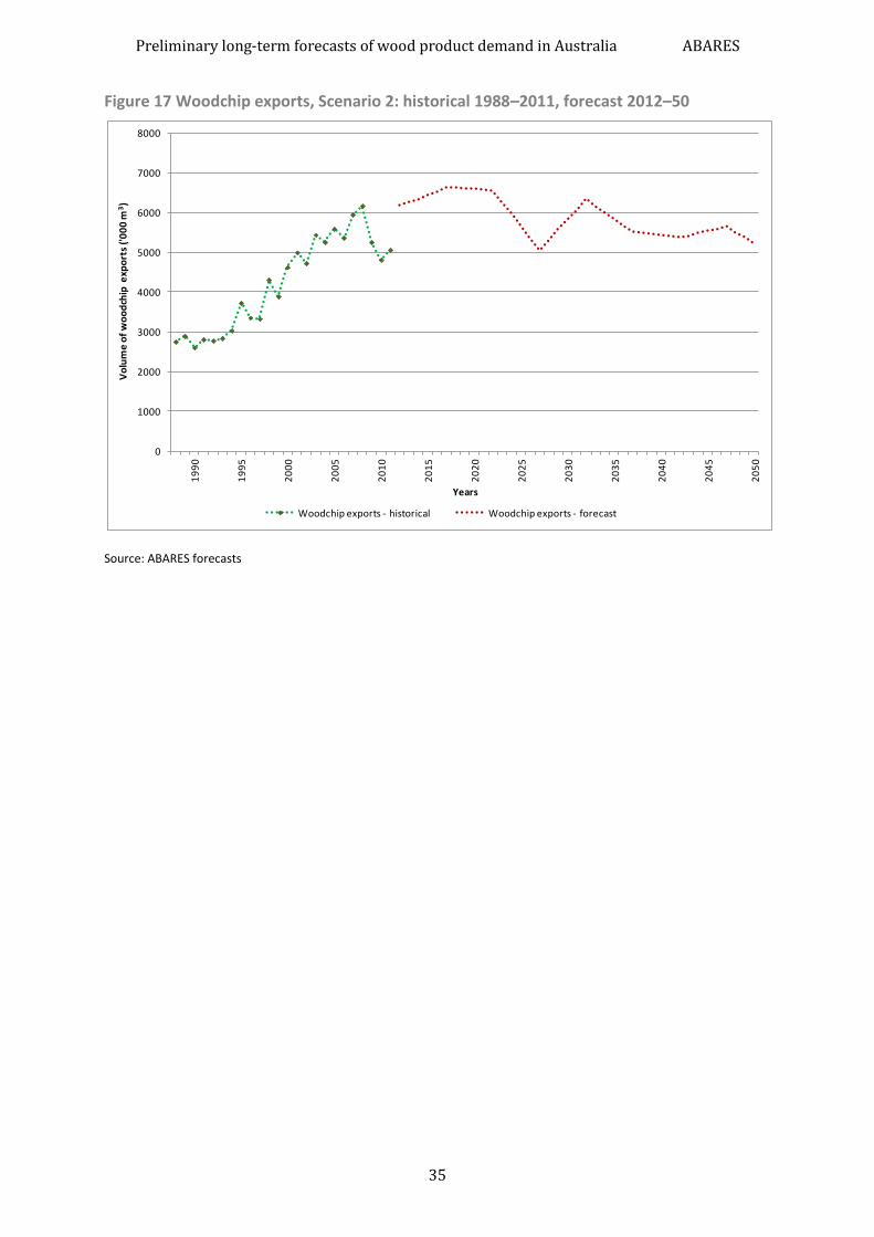
Preliminary long-term forecasts of wood product demand in Australia ABARES
35
Figure 17 Woodchip exports, Scenario 2: historical 1988–2011, forecast 2012–50
Source: ABARES forecasts
0
1000
2000
3000
4000
5000
6000
7000
8000
19
90
19
95
20
00
20
05
20
10
20
15
20
20
20
25
20
30
20
35
20
40
20
45
20
50
Vo
lum
e o
f w
oo
dch
ip e
xpo
rts
('0
00
m3)
Years
Woodchip exports - historical Woodchip exports - forecast

Preliminary long-term forecasts of wood product demand in Australia ABARES
36
8 Summarising forecasts of consumption and trade
ABARES estimates that sawnwood consumption will continue to increase to 2049–50, although
more slowly than consumption of other wood products. This growth will be driven by ongoing
growth in detached and multi-dwelling commencements, underpinned by Australia’s population
growth. Sawnwood consumption is forecast to increase from 5.0 million cubic metres in
2010–11 to 6.0 million cubic metres in 2029–30 and 6.5 million cubic metres in 2049–50.
ABARES preliminary forecasts indicate that sawnwood consumption will continue to increase to
2049–50, albeit more slowly than consumption of other wood products, driven by ongoing
growth in detached and multi-dwelling commencements, underpinned by Australia’s population
growth. Sawnwood consumption is forecast to increase from 5.0 million cubic metres in
2010–11 to 6 million cubic metres in 2029–30 and 6.5 million cubic metres in 2049–50. While
sawnwood consumption in Australia declined by an average of 0.5 per cent a year over 2001–11,
the forecasts in this report project sawnwood consumption to grow by 0.6 per cent a year on
average between 2011–12 and 2049–50 (Figure 18). Sawnwood imports are also forecast to
increase, growing by 1.5 per cent a year on average between 2011–12 and 2049–50. This is
driven by the rise in multi-dwelling commencements and an assumed stable Australian–US
dollar exchange rate. Sawnwood consumption per capita falls over the forecast period and the
proportion of sawnwood imports to consumption rises, averaging 22.4 per cent between 2044–
45 and 2048–49.
Figure 18 Sawnwood consumption and imports, historical 2000–11, forecasts 2012–50
Note: The height of the grey (historical) and red (forecasts) columns represents the total volume of sawnwood consumed
(left axis). Historical data (2000–11) for sawnwood imports is shown in light grey. Forecasts (2012–50) for sawnwood
imports are shown in orange. Consumption of sawnwood per capita is shown on the right axis in green. The models for
0.00
0.05
0.10
0.15
0.20
0.25
0.30
0.35
0
1000
2000
3000
4000
5000
6000
7000
20
00
20
05
20
10
20
15
20
20
20
25
20
30
20
35
20
40
20
45
20
50
Saw
nw
oo
d c
on
sum
pti
on
pe
r ca
pit
a (m
3p
er
pe
rso
n)
Vo
lum
e in
'000
m3
Years
Sawnwood imports (H) Share of consumption from domestic production (H)
Sawnwood imports (F) Share of consumption from domestic production (F)
Consumption per capita (RH axis)

Preliminary long-term forecasts of wood product demand in Australia ABARES
37
consumption and imports were constructed independently of each other and did not account for the definition of apparent
consumption when forecasting. Hence it is not possible to make any inferences for changes in domestic production and
exports. It is however possible to conclude that the area in red shows the forecast share of consumption from domestic
production to 2049–50.
Source: ABARES forecasts
ABARES estimates that wood-based panel consumption will continue to increase over the
forecast period, driven by growth in multi-dwelling commencements and alterations and
additions, both of which are underpinned by population growth in capital cities. Consumption of
wood-based panels is forecast to increase by an average of 2 per cent a year, from 2.0 million
cubic metres in 2010–11 to 3.1 million cubic metres in 2029–30 and 4.3 million cubic metres in
2049–50 (Figure 19). This is lower than historical growth in consumption, which grew by
3.6 per cent a year on average between 2000–01 and 2010–11. Wood-based panel imports are
forecast to grow at a slower rate, averaging 0.8 per cent a year between 2010–11 and 2049–50.
Wood-based panel consumption per capita rises over the forecast period and the proportion of
imports to consumption falls, averaging around 12.4 per cent between 2044–45 and 2048–49.
Figure 19 Wood-based panel consumption and imports, historical 2000–11, forecasts 2012–50
Note: The height of the grey (historical) and red (forecasts) columns represents the total volume of wood-based panels
consumed (left axis). Historical data (2000–11) for wood-based panel imports is shown in light grey. Forecasts (2012–50) for
wood-based panel imports are shown in orange. Consumption of wood-based panels per capita is shown on the right axis in
green. The models for consumption and imports were constructed independently of each other and did not account for the
definition of apparent consumption when forecasting. Hence it is not possible to make any inferences for changes in
domestic production and exports. However, it is possible to conclude that the area in red shows the forecast share of
consumption from domestic production to 2049–50.
Source: ABARES forecasts
0.00
0.02
0.04
0.06
0.08
0.10
0.12
0.14
0
500
1000
1500
2000
2500
3000
3500
4000
4500
5000
20
00
20
05
20
10
20
15
20
20
20
25
20
30
20
35
20
40
20
45
20
50
Wo
od
-bas
ed
pan
el c
on
sum
pti
on
pe
r cap
ita
(m3
pe
r pe
rso
n)
Vo
lum
e in
'000
m3
Years
Wood-based Panels Imports (H) Share of consumption from domestic production (H)
Wood-based Panels Imports (F) Share of consumption from domestic production (F)
Consumption per capita (RH axis)

Preliminary long-term forecasts of wood product demand in Australia ABARES
38
Paper and paperboard consumption is forecast to grow at a faster rate than imports. ABARES
estimates that paper and paperboard consumption will increase from 4.0 million tonnes in
2010–11 to 5.8 million tonnes in 2029–30 (averaging 1.9 per cent a year between 2010–11 and
2029–30) and reaching 7.1 million tonnes in 2049–50 (averaging 1 per cent a year between
2029–30 and 2049–50). These forecasts are based largely on ABARES projections for value
added by the manufacturing sector. The manufacturing sector is a large user of packaging and
industrial paper and printing and writing paper and represents a domestic demand factor.
Growth in paper and paperboard imports is expected to increase marginally from around 2 per
cent between 2000–01 and 2010–11 to an average of 2.2 per cent between 2010–11 and
2049–50 (Figure 20). Paper and paperboard consumption per capita rises over the forecast
period and the proportion of paper imports to consumption rises averaging around 59.8 per
cent between 2044–45 and 2048–49.
Figure 20 Paper and paperboard consumption and imports, historical 2000–11, forecasts 2012–50
Note: The height of the grey (historical) and red (forecasts) columns represents the total volume of paper and paperboard
products consumed. Historical data (2000–11) for paper imports is shown in light grey. Forecasts (2012–50) for paper
imports are shown in orange. Consumption of paper and paperboard products per capita is shown on the secondary axis in
green. The models for consumption and imports were constructed independently of each other and did not account for the
definition of apparent consumption when forecasting. Hence it is not possible to make any inferences for changes in
domestic production and exports. However, it is possible to conclude that the area in red shows the forecast share of
consumption from domestic production to 2049–50.
Source: ABARES forecasts
Consumption per capita is a useful indicator: a stronger growth in consumption of a wood
product than in population suggests an increase in use and demand for that product. The results
imply an increased demand for wood-based panel and paper and paperboard products. In
160
165
170
175
180
185
190
195
200
205
210
0
1000
2000
3000
4000
5000
6000
7000
8000
20
00
20
05
20
10
20
15
20
20
20
25
20
30
20
35
20
40
20
45
20
50 Pap
er a
nd
pap
erb
oar
d c
on
sum
pti
on
pe
r ca
pit
a ( t
on
ne
s p
er
pe
rso
n)
Vo
lum
e in
kt
Years
Paper and Paperboard Imports (H) Share of consumption from domestic production (H)
Paper and Paperboard Imports (F) Share of consumption from domestic production (F)
Consumption per capita
(RH axis)

Preliminary long-term forecasts of wood product demand in Australia ABARES
39
contrast, while consumption of sawnwood is forecast to increase, consumption per capita is
estimated to decrease.
Further, the mean proportion of imports to consumption is forecast to fall for wood-based
panels (Table 13) and is forecast to rise for sawnwood and paper and paperboard products
between 2011–12 and 2049–50 (Table 8, Table 18). However, import and consumption models
have been constructed independently and it is difficult to make inferences for domestic
production and export facilities based on these results. The implications of these findings for
additional investment in domestic processing capacity will depend on a number of factors, such
as future parameters affecting domestic and international processing competitiveness as well as
government policies. Domestic investment and processing is not necessarily more efficient, from
an economic perspective, than exporting raw materials and importing final products; although
they may imply vastly divergent outlooks for Australia’s forestry industry, and have different
social and environmental implications.
A substantial share of Australia’s current wood processing capacity includes woodchip
production for export. Forecasts of pulplog availability have been compiled from ABARES
publicly available datasets. Based on the estimated growth in pulplog availability, additional
domestic infrastructure capacity may be needed for these logs. This investment may result in
capacity to process domestically or additional exports of unprocessed logs and woodchips
following recent trends in domestic woodchip production. For example, the volume of plantation
pulplogs harvested from hardwood forests for woodchip exports has increased by around 31 per
cent from 3.6 million cubic metres in 2006–07 to 4.7 million cubic metres in 2010–11. A
scenario considered to be an upper bound is examined in this report by assuming constant
domestic production of paper and paperboard and wood-based panels (that is, no further
investment in capacity to process logs domestically). Under this scenario, woodchip exports are
forecast to increase from 5.1 million cubic metres in 2010–11 to 6.5 million cubic metres in
2029–30 (averaging a 1.5 per cent increase per year between 2010–11 and 2029–30) and
remain stable thereafter to around 6.5 million cubic metres in 2049–50 (averaging a zero
increase per year between 2029–30 and 2049–50). This trend in woodchip exports is primarily
driven by the forecast increase in availability and harvest of pulplogs.
An alternative scenario is investigated by assuming constant exports of paper and panel
products which allows estimation of domestic production as the gap between forecast
consumption and imports. This scenario assumes there is scope for new investment in
additional paper and paperboard processing and wood-based panel manufacturing capacity in
Australia. Under this scenario, woodchip exports are forecast to increase from 5.1 million cubic
metres in 2010–11 to 5.8 million cubic metres in 2029–30 (averaging a 0.9 per cent increase per
year between 2010–11 and 2029–30) and decrease to 5.2 million cubic metres in 2049–50
(averaging a 0.5 per cent decline each year between 2030–31 and 2049–50). The trend in
woodchip exports is driven by the forecast for total pulplogs harvested and influenced by the
volume of pulplogs used for domestic production of paper and panels. Woodchip exports are
forecast to fall between 2029–30 and 2049–50 due to growth in consumption of wood-based
panels and a decrease in the proportion of imports to consumption. This combined with steady
growth in paper and paperboard consumption results in higher domestic panel and paper
production and consequently higher domestic demand for pulplogs during a period where
pulplogs available for harvest are projected to decrease.

Preliminary long-term forecasts of wood product demand in Australia ABARES
40
Range of forecasts
Consumption and trade of sawnwood, wood-based panels, paper and paperboard and
woodchips is forecast based on business-as-usual assumptions made in this report. The
uncertainty associated with these forecasts is largely a function of unaccounted variation as well
as variation in modelled factors. This uncertainty is represented by the 95 per cent confidence
intervals which provide a range for the forecast with 95 per cent certainty under business-as-
usual assumptions. However, as noted in previous caveats, the range provided by the 95 per cent
confidence interval limits the variability of exogenous parameters and does not allow for
potential future errors in the assumptions.
It is important to acknowledge that business-as-usual assumptions limit the potential variability
in factors used in the forecasting models. While the forecast for sawnwood consumption in
2049–50 is 6.5 million cubic metres, the 95 per cent confidence interval suggests a range for this
forecast of between 5.5 and 7.4 million cubic metres (Table 24). Similarly, wood-based panel
consumption in 2049–50 is forecast to be 4.3 million cubic metres but may range between
3.6 and 5.1 million cubic metres. The housing industry is a large user of structural wood; thus
the forecast trend in sawnwood and wood-based panel consumption is primarily driven by
dwelling commencements. Paper and paperboard consumption is primarily driven by the value
added by the manufacturing sector which is forecast to increase by 20.4 per cent in 2049–50
relative to 2010–11 (ABARES projections discussed in Appendix B). As a result, paper
consumption is forecast to be 7.1 million cubic metres in 2049–50, ranging between 6.2 and
8.0 million cubic metres.
Table 24 Summary of forecasts for consumption and trade of selected wood products, 2010–11 to 2049–50
Units 2010–11 2029–30 f 2049–50 f Consumption Estimate 95% CI Estimate 95% CI Sawnwood ’000 m3 5 047 5 984 ± 831 6 475 ± 924 Wood-based panels ’000 m3 2 048 3 126 ± 497 4 341 ± 715 Paper and paperboard ’000 tonnes 4 012 5 774 ± 715 7 083 ± 932 Imports Sawnwood ’000 m3 846 1 225 ± 357 1 481 ± 438 Wood-based panels ’000 m3 407 460 ± 161 539 ± 194 Paper and paperboard ’000 tonnes 1 886 3 184 ± 648 4 281 ± 890 Exports Scenario 1 Scenario 2 Scenario 1 Scenario 2 Woodchip exports ’000 m3 5 064 6 479 5 816 6 455 5 222
Note: CI =confidence interval, f ABARES forecast
In this report ABARES explored the effect of two scenarios for domestic processing to provide an
estimate for woodchip exports. In Scenario 1 no further investment was assumed in domestic
processing which led to an increase in the volume of woodchip exports over the forecast period.
In Scenario 2 woodchips are increasingly used domestically with an expansion in the domestic
processing of paper products and manufacturing of panel products, leading to a decline in the
volume of woodchip exports over the forecast period.
As demonstrated by these restricted scenarios, a number of factors need to be taken into
account when analysing potential investment in processing capacity and domestic use of
pulplogs over time. Many factors can affect domestic investment and production decisions and
will have implications for viability of harvesting logs for woodchips compared with other uses.
These forecasts would be different for alternative assumptions about:
production of paper, pulp and panels in Australia

Preliminary long-term forecasts of wood product demand in Australia ABARES
41
substitution of logs with other fibres
opportunities for alternative markets such as bioenergy.
Other issues not considered in this analysis include changes to overseas demand for Australian
woodchips and long-term social and environmental values. Future research in forecasting the
long-term outlook for Australia’s forestry industry could examine these considerations and
assess the potential domestic processing capacity of Australia’s forecast log availability.
Further research
In this report, ABARES analysed consumption and imports of wood products and highlighted
broad trends across the forestry sector. However, more sophisticated analysis of domestic
production is needed to adequately assess the long-term implications of the forecast surplus in
log availability. In particular, whether log availability could translate into additional investments
in domestic processing capacity would depend on a number of factors that need to be
considered within a comprehensive modelling framework.
Further ABARES research could include investigation of additional explanatory variables in the
econometric models, and breakdown of commodity forecasts into their detailed components. A
reduced form econometric analysis could also be examined to create a model structure wherein
the level of consumption implicitly helps determine the level of imports. In future research
ABARES could also integrate consumption and trade forecasts with FORUM to produce regional
estimates of wood products output and investment over the forecast period. The log equivalent
consumption implied by the forecasts in this report can also be explored. Combined with the
outputs of FORUM, a comparison with projections for availability of different sawlog and pulplog
grades could provide insights to trends in production of different commodity groups. This
comparison could also provide a better understanding of the importance of trade. While
Australia’s forecast log availability may exhibit substantial growth in some areas, existing
processing capacity may not be sufficient to process larger log volumes. Future research using
FORUM could assess the economic potential for investments in processing capacity over time,
taking into account the availability of timber as well as the volume of imports.
Future analysis could also include development and modelling of alternative outlook scenarios
for the forestry sector. These scenarios could include sets of assumptions that define alternative
futures for Australia’s wood product industries, different assumptions for economic and
population growth, regulations and market incentives for investments in timber resources and
processing infrastructure, and demand conditions for wood products.

Preliminary long-term forecasts of wood product demand in Australia ABARES
42
Appendix A: Econometric models for consumption and trade of wood products ABARES has, for many years, produced short-term forecasts of sawnwood, wood-based panels
and paper and paperboard for its Agricultural Commodities report, as well as ad hoc forecasts for
specific research reports (such as Love et al. 1999). The Agricultural Commodities forecasts are
undertaken using a simplified approach, based on aggregate commodity groups (sawnwood and
wood-based panels and paper and paperboard). These forecasts have generally focused on
exports and imports primarily using trend analysis to estimate unit values and the value of trade
flows and are informed by some econometric modelling of the volume of trade.
As part of this report, ABARES developed a long-term econometric forecasting methodology,
jointly funded by Forest and Wood Products Australia (FWPA) and ABARES, that represents a
more comprehensive and sophisticated approach more closely aligned to that taken in the ad
hoc research reports such as Love and colleagues (1999). The current approach involved setting
up regression models for consumption of wood products, which estimate the relationships
between dependent variables and the respective factors that help determine them
(independent/explanatory variables). These models were estimated using the econometric and
forecasting software, EViews. Historical data for consumption is calculated using the definition
of apparent consumption. The apparent consumption of wood products is calculated as:
For the present analysis, the consumption forecasting models encompass a 39-year time horizon
from 2011–12 to 2049–50. The present forecasting research also includes development of wood
product trade models, which employ more comprehensive frameworks, as discussed in this
appendix, than currently used for the Agricultural Commodities forecasts. Given the relationship
between consumption and imports, the trade models would ideally incorporate the definition of
apparent consumption using a reduced form econometric analysis to determine imports as
described in Appendix C. However, as outlined in Appendix C, this approach requires an
exogenous projection for production and exports. Future research and analysis using FORUM
may test this methodology in greater detail.
It is worth mentioning the difference between the economic model and the econometric model
discussed in this appendix. The economic model is a hypothesis that looks at a number of
variables that may help forecast the dependent variable. These variables were extensively tested
and either included or discarded in the econometric model. The econometric model is the result
of considerable testing of hypothesised variables and includes variables to account for business
cycle components and outliers or influential points in the data. Prices while hypothesised to
explain the volume of consumption and imports were not included in the modelling process due
to limited reliability and availability of data.
Sawnwood and wood-based panels
Methodology
It is expected that consumption of structural timber is primarily a function of housing starts and
other macroeconomic variables. Given that a significant percentage of sawnwood and wood-
based panel consumption is used for structural purposes, detached and multi-dwelling housing

Preliminary long-term forecasts of wood product demand in Australia ABARES
43
starts and alterations or additions to existing homes (or renovations) are likely to be the major
demand factors in the consumption model. However, housing starts and renovations alone may
be insufficient to fully explain wood consumption levels during economic contractions or
business cycles. Macroeconomic variables such as real GDP per capita, home loan interest rates
and population growth or variables accounting for dynamic patterns such as auto-regressive or
moving average terms may also affect the forecasts of consumption and trade.
The forecasts for imports are likely to be affected by domestic demand in Australia and may
additionally depend on macroeconomic variables for Australia’s major trading partners. The
import model may also be influenced by domestic/world GDP growth and world prices.
ABARES developed a set of econometric models to project domestic consumption of sawnwood
and wood-based panels. Development of these models involved identifying the factors likely to
affect timber consumption, and regression analysis of these variables. The full potential of the
constructed models lies in estimating consumption until 2050, thereby providing a long-term
picture of the market and direction for the sawnwood and panels industries.
The hypothesis for the economic model is that sawnwood consumption is a function of housing
starts and other macroeconomic variables. The econometric model, based on rigorous testing,
may take some or all of these variables into account.
Where:
swc is total consumption of sawnwood (hardwood sawnwood and softwood sawnwood)
DD is commencements of detached dwellings
MD is commencements of multi-dwellings
RGDPP is real gross domestic product per capita
HINT is home loan interest rates
POP is population
HINC is household income.
The economic model for wood-based panel consumption was hypothesised to be a function of
housing starts, the value of renovations and other macroeconomic variables. It is expected that
wood-based panel consumption is primarily for use in multi-dwelling commencements. The
econometric model, based on rigorous testing, may take some or all of these variables into
account.
Where:
wbpc is total consumption of wood-based panels (plywood, particleboard and medium density fibreboard)
MD is commencements of multi-dwellings
RENO is value of renovations
RGDPP is real gross domestic product per capita
HINC is household income.

Preliminary long-term forecasts of wood product demand in Australia ABARES
44
ABARES also developed a set of econometric models to forecast imports of sawnwood and
wood-based panels. Development of these models relies primarily on domestic demand factors,
macroeconomic factors and moving average terms accounting for dynamic patterns. This
analysis significantly improves past forecast methodologies for the Agricultural Commodities
report. Previous reports (including Love et al. 1999) did not fit econometric models for
estimation of trade. As with consumption, the full potential of this analysis lies in estimating
imports to 2050.
The economic model hypothesised for sawnwood imports was a function of housing starts and
some domestic and international macroeconomic factors. The econometric model, based on
rigorous testing, may take some or all of these variables into account.
New Zealand’s real GDP per capita was included in the hypothesis as New Zealand is one of
Australia’s key trading partners for wood products. Trends in New Zealand’s economy can play a
role in determining trade and hence consumption in Australia.
Where:
swi is imports of sawnwood
DD is commencements of detached dwellings
MD is commencements of multi-dwellings
RGDPP is Australia’s real gross domestic product per capita
POP is population
USEX is Australian to US dollar exchange rate
NZRGDPP is New Zealand’s real gross domestic product per capita.
In a similar fashion, wood-based panel imports were hypothesised to be a function of housing
starts and macroeconomic variables. The econometric model, based on rigorous testing, may
take some or all of these variables into account.
Where:
swi is imports of sawnwood
MD is commencements of multi-dwellings
RENO is value of renovations
RGDPP is Australia’s real gross domestic product per capita
POP is population
USEX is Australian to US dollar exchange rate.
Possible time trend, stationarity and increasing volatility issues were considered and tested
using the auto-correlation function (ACF), Partial ACF and Augmented Dickey Fuller (ADF) tests.
On completion of these tests it was found that unit root issues were present in most variables
requiring us to take the first difference of the data. Further, the log of all variables was taken to
enable additional interpretation of coefficients. Two potential outliers in the data, in 1983 (due
to a significant drought) and in 2000 (due to imminent introduction of the Goods and Services
Tax or GST) were found with varying effects on the identified variables (Figure A1).
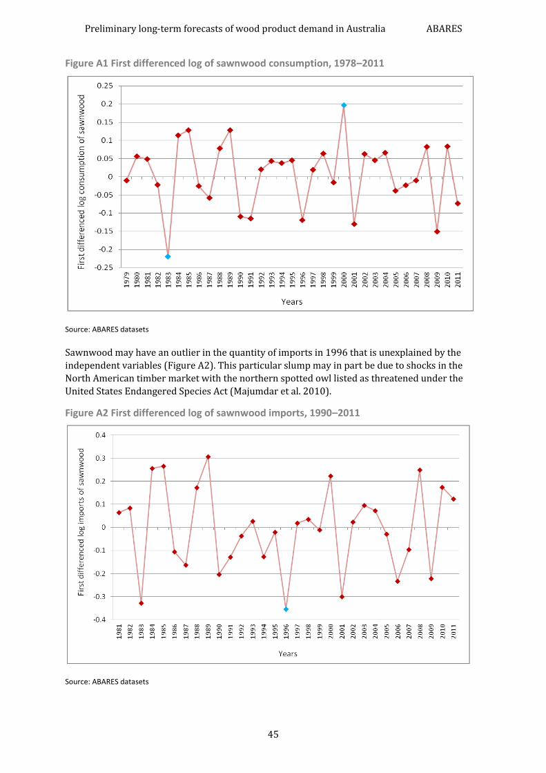
Preliminary long-term forecasts of wood product demand in Australia ABARES
45
Figure A1 First differenced log of sawnwood consumption, 1978–2011
Source: ABARES datasets
Sawnwood may have an outlier in the quantity of imports in 1996 that is unexplained by the
independent variables (Figure A2). This particular slump may in part be due to shocks in the
North American timber market with the northern spotted owl listed as threatened under the
United States Endangered Species Act (Majumdar et al. 2010).
Figure A2 First differenced log of sawnwood imports, 1990–2011
Source: ABARES datasets

Preliminary long-term forecasts of wood product demand in Australia ABARES
46
A potential outlier in wood-based panel consumption was found in 1993 when medium density
fibreboard consumption was first recorded in Australia (Figure A3).
Figure A3 First differenced log of wood-based panel consumption, 1990–2011
Source: ABARES datasets
A potential outlier in wood-based panel import quantities was found in 2000 just before the GST
was introduced in Australia (Figure A4).
Figure A4 First differenced log of wood-based panel imports, 1990–2011
Source: ABARES datasets

Preliminary long-term forecasts of wood product demand in Australia ABARES
47
The consumption and trade forecasting model used ordinary least squares (OLS) methods as
there was no evidence to suggest a need for non-linear least squares. This follows the same
procedure as that of Love and colleagues (1999) and Hossain and colleagues (1989) who both
used OLS estimation, forecasting approximately 40 years. In this report the structure of the
models has been improved to avoid challenges faced by earlier reports and better model the
dynamic and business cycle components of the data.
Econometric results
Sawnwood consumption
3
(0.049) (0.048) (0.024)
3 7
(0.026) (0.052)
5 3
Where:
is sawnwood consumption in thousand cubic metres
is the number of detached dwellings commenced
is the number of multi-dwellings commenced
and are dummy variables for 2000 and 2002
MA is a moving average term.
The purpose of the model is to establish and test the hypothesised relationship between the
number of detached and multi-dwellings commenced and sawnwood consumption. Hence,
specific outliers in consumption were separated to observe the effect of dwelling
commencements on sawnwood consumption.
The model was constructed on first differenced log data. A dummy variable was used for an
outlier in consumption levels in 2000 when the goods and services tax (GST) was introduced to
Australia. A dummy variable in 2002 reflects a significant increase in detached and multi-
dwelling commencements following the temporary slump in 2000–01 following introduction of
the GST. The moving average term accounts for dynamic patterns in consumption between 1979
and 2011 which are assumed to continue to 2050.
The fitted model follows actual data accurately and within a 95 per cent confidence interval. The
model was tested for stability in residuals and forecasts. It appears stable with a high adjusted
R-squared value, significant explanatory variables and consistent t-statistics (Table A1). While
the Durbin–Watson statistic is low, rigorous testing indicates stability in the residuals with no
detection of serial correlation or heteroskedasticity issues. Tests were also undertaken for
multicollinearity and co-integration with negative results.

Preliminary long-term forecasts of wood product demand in Australia ABARES
48
Table A1 Sawnwood consumption model: EViews output
The model estimated in EViews suggests a positive coefficient for multi-dwelling and detached
dwelling commencements (explanatory variables). Therefore a positive change in the
explanatory variables results in a corresponding positive change in the quantity of sawnwood
consumption. The coefficients in the model estimate the extent of the change. As these models
are constructed in first difference logs, the coefficient approximates a percentage change.
Specifically, a 1 per cent increase in detached or multi-dwelling commencements is estimated to
result in a 0.12 per cent and 0.32 per cent increase in sawnwood consumption, respectively.
Sawnwood imports
1 4
(0.132) (0.186)
2
(0.066) (0.036)
1 4
Where:
is sawnwood imports in thousand cubic metres
is the number of multi-dwellings commenced
is the Australian to US dollar exchange rate
is a dummy variable for 1996
is a moving average term.
The purpose of the model is to establish and test the hypothesised relationship between the
number of multi-dwelling commencements, the Australian to US dollar exchange rate and
Dependent Variable: D(LOG(SWC))
Method: Least Squares
Sample (adjusted): 1979 2011
Included observations: 33 after adjustments
Convergence achieved after 15 iterations
MA Backcast: 1974 1978 Variable Coefficient Std. Error t-Statistic Prob. D(LOG(DD)) 0.124276 0.048657 2.554152 0.0164
D(LOG(MD)) 0.317249 0.048035 6.604555 0.0000
D00 0.162751 0.023835 6.828138 0.0000
D02 -0.092510 0.026455 -3.496935 0.0016
MA(5) -0.869993 0.051647 -16.84483 0.0000 R-squared 0.908434 Mean dependent var 0.005943
Adjusted R-squared 0.895353 S.D. dependent var 0.091706
S.E. of regression 0.029666 Akaike info criterion -4.058889
Sum squared resid 0.024642 Schwarz criterion -3.832146
Log likelihood 71.97168 Hannan-Quinn criter. -3.982597
Durbin-Watson stat 1.299795 Inverted MA Roots .97 .30-.92i .30+.92i -.79+.57i
-.79-.57i

Preliminary long-term forecasts of wood product demand in Australia ABARES
49
sawnwood imports. Hence, specific outliers in imports were separated to observe the effect of
the explanatory variables on sawnwood imports. The model was constructed on first differenced
log data. A dummy variable was used for outlying import levels in 1996. It is possible that this
reflects a restructuring of imports from the North American region due to environmental
regulations implemented around this time.
The moving average term accounts for dynamic patterns in imports between 1990 and 2011
which are assumed to continue to 2050.
The fitted model follows the actual data accurately and within a 95 per cent confidence interval.
The model was tested for stability in residuals and forecasts. It appears stable with good
adjusted R-squared value, significant explanatory variables, consistent t-statistics and Durbin–
Watson statistic (Table A2). Testing further shows stability in the residuals with no detection of
serial correlation or heteroskedasticity. Tests were also undertaken for multicollinearity and
co-integration with negative results.
Table A2 Sawnwood imports model: EViews output
The model estimated in EViews suggests a positive coefficient for multi-dwelling
commencements and the Australian to US dollar exchange rate (explanatory variables).
Therefore a positive change in the explanatory variables results in a corresponding positive
change in the quantity of sawnwood imports. The coefficients in the model estimate the extent of
the change. As these models are constructed in first difference logs, the coefficient approximates
a percentage change. Specifically, a 1 per cent increase in multi-dwelling commencements or
Australian to US dollar exchange rates is estimated to result in a 0.74 per cent and 0.32 per cent
increase in sawnwood imports, respectively.
Dependent Variable: D(LOG(SWI))
Method: Least Squares
Sample (adjusted): 1990 2011
Included observations: 22 after adjustments
Convergence achieved after 9 iterations
MA Backcast: 1984 1989 Variable Coefficient Std. Error t-Statistic Prob. D(LOG(MD)) 0.740904 0.131906 5.616914 0.0000
D(LOG(US_EX)) 0.323939 0.185682 1.744591 0.0981
D96 -0.153216 0.065732 -2.330935 0.0316
MA(6) -0.911921 0.036484 -24.99510 0.0000 R-squared 0.906147 Mean dependent var -0.032365
Adjusted R-squared 0.890505 S.D. dependent var 0.162795
S.E. of regression 0.053869 Akaike info criterion -2.841560
Sum squared resid 0.052234 Schwarz criterion -2.643189
Log likelihood 35.25716 Hannan-Quinn criter. -2.794830
Durbin-Watson stat 1.724113 Inverted MA Roots .98 .49-.85i .49+.85i -.49-.85i
-.49+.85i -.98

Preliminary long-term forecasts of wood product demand in Australia ABARES
50
Wood-based panel consumption
2 8
(0.053) (0.038) (0.045)
5 7
(0.039) (0.036)
8
Where:
is wood-based panel consumption in thousand cubic metres
is the number of multi-dwellings commenced
is the value of approved alterations and additions to existing dwellings in thousands of 2010 Australian dollars
and are dummy variables for 1989 and 1993
is a moving average term.
The purpose of the model is to establish and test the hypothesised relationship between number
of multi-dwellings commenced, value of renovations and wood-based panel consumption.
Hence, specific outliers in consumption were separated to observe the effect of these factors on
wood-based panel consumption.
The model was constructed on first differenced log data. A dummy variable for outlying
consumption levels was used in 1989. This coincides with deregulation of financial markets in
Australia and a false recovery from recession in 1987. A dummy variable was also used for
consumption levels in 1993. This accounts for the increase in wood-based panel consumption
levels when medium density fibreboard consumption was first estimated in Australia.
The fitted model follows the actual data accurately and within a 95 per cent confidence interval.
The model was tested for stability in residuals and forecasts. It appears stable with a high
adjusted R-squared value, significant explanatory variables, consistent t-statistics and Durbin–
Watson statistic (Table A3). Testing further shows stability in the residuals with no detection of
serial correlation or heteroskedasticity. Tests were also undertaken for multicollinearity and
co-integration with negative results.

Preliminary long-term forecasts of wood product demand in Australia ABARES
51
Table A3 Wood-based panels consumption model: EViews output
The model estimated in EViews suggests a positive coefficient for both multi-dwelling
commencements and the value of renovations. Therefore a positive change in explanatory
variables results in a corresponding positive change in quantity of wood-based panels
consumed. The coefficients in the model estimate the extent of the change. As these models are
constructed in first difference logs, the coefficient approximates a percentage change.
Specifically, a 1 per cent increase in multi-dwelling commencements results in a 0.26 per cent
increase in the rate of growth in wood-based panel consumption. Similarly, a 1 per cent increase
in the value of renovations results in a 0.48 per cent increase in wood-based panel consumption.
Wood-based panel imports
5 6
(0.082) (0.094) (0.080)
(0.071) (0.042)
2
Where:
is wood-based panel imports in thousand cubic metres
is the number of multi-dwellings commenced
and are dummy variables for 1995, 2000 and 2007
is a moving average term.
The purpose of the model is to establish and test the hypothesised relationship between the
number of multi-dwellings commenced and wood-based panel imports. Hence, specific outliers
in imports were separated to observe the effect of these factors on wood-based panel imports.
Dependent Variable: D(LOG(WBPC))
Method: Least Squares
Sample (adjusted): 1979 2011
Included observations: 33 after adjustments
Convergence achieved after 11 iterations
MA Backcast: 1975 1978 Variable Coefficient Std. Error t-Statistic Prob. D(LOG(RENO)) 0.481512 0.052704 9.136079 0.0000
D(LOG(MD)) 0.263182 0.037788 6.964722 0.0000
D89 0.097721 0.045229 2.160588 0.0394
D93 0.249939 0.039017 6.405863 0.0000
MA(4) -0.877220 0.036440 -24.07310 0.0000 R-squared 0.918739 Mean dependent var 0.041752
Adjusted R-squared 0.907131 S.D. dependent var 0.123093
S.E. of regression 0.037512 Akaike info criterion -3.589580
Sum squared resid 0.039400 Schwarz criterion -3.362836
Log likelihood 64.22806 Hannan-Quinn criter. -3.513287
Durbin-Watson stat 2.052249 Inverted MA Roots .97 .00-.97i -.00+.97i -.97

Preliminary long-term forecasts of wood product demand in Australia ABARES
52
The model was constructed on first differenced log data. Dummy variables for outliers in the
quantity of imports were used in 1995, 2000 and 2007. The moving average term accounts for
dynamic patterns in imports between 1990 and 2011 which are assumed to continue to 2050.
The fitted model follows the actual data accurately and within a 95 per cent confidence interval.
The model was tested for stability in residuals and forecasts. It appears stable with an
acceptable adjusted R-squared value, significant explanatory variables, consistent t-statistics
and Durbin–Watson statistic (Table A4). Testing further shows stability in the residuals with no
detection of serial correlation or heteroskedasticity. Tests were also undertaken for
multicollinearity and co-integration with negative results.
The model estimated in EViews suggests a positive coefficient for the number of multi-dwellings
commenced (explanatory variable). Therefore a positive change in the explanatory variable
results in a corresponding positive change in the quantity of wood-based panels imported. The
coefficients in the model estimate the extent of the change. As these models are constructed in
first difference logs, the coefficient approximates a percentage change. Specifically, a 1 per cent
increase in multi-dwelling commencements is estimated to result in a 0.62 per cent increase in
wood-based panel imports.
Table A4 Wood-based panel imports model: EViews output
Paper and paperboard
Methodology
ABARES identified the range of potential factors affecting long-term consumption and import of
paper and paperboard based on economic theory and a literature review of similar studies.
Although the models described in this report provide forecasts for consumption and import of
aggregate paper and paperboard, rather than individual paper grades, ABARES considered the
factors affecting these components in estimating the drivers of total consumption and trade.
Dependent Variable: D(LOG(WBPI))
Method: Least Squares
Sample (adjusted): 1990 2011
Included observations: 22 after adjustments
Convergence achieved after 12 iterations
MA Backcast: 1985 1989 Variable Coefficient Std. Error t-Statistic Prob. D(LOG(MD)) 0.618372 0.082179 7.524714 0.0000
D00 0.259966 0.079933 3.252300 0.0047
D07 0.186067 0.070709 2.631447 0.0175
D95 0.224612 0.094049 2.388256 0.0288
MA(5) -0.878317 0.042423 -20.70379 0.0000 R-squared 0.815324 Mean dependent var 0.045131
Adjusted R-squared 0.771871 S.D. dependent var 0.151685
S.E. of regression 0.072449 Akaike info criterion -2.215154
Sum squared resid 0.089230 Schwarz criterion -1.967189
Log likelihood 29.36669 Hannan-Quinn criter. -2.156741
Durbin-Watson stat 2.194668 Inverted MA Roots .97 .30-.93i .30+.93i -.79+.57i
-.79-.57i

Preliminary long-term forecasts of wood product demand in Australia ABARES
53
ABARES developed a set of econometric models to project domestic consumption and imports of
paper and paperboard. Development of these models involved identifying a primary demand
variable and other macroeconomic variables likely to affect consumption and trade, and
regression analysis of these variables. The full potential of the constructed models lies in
estimating consumption and imports until 2050, thereby providing a more complete picture of
the market and direction for the paper and paperboard industry.
Paper and paperboard consumption and imports were hypothesised to be a function of the value
of the output of the manufacturing sector in Australia and other macroeconomic variables. The
econometric model, based on rigorous testing, may take some or all of these variables into
account.
Where:
ppbc is total consumption of paper and paperboard (newsprint, printing and writing, packaging and industrial, and household and sanitary paper)
MANF is the value added by manufacturing sector
RGDPP is real gross domestic product per capita
POP is population
CINC is consumer income
ppbi is total imports of paper and paperboard
PRICEWORLD is the world price of paper and paperboard
USRGDPP is the United States real gross domestic product per capita.
It was not possible, due to time and data limitations, to estimate and test the relationship
between all identified potential factors and paper and paperboard consumption and imports.
For example, consumption of newsprint may be affected by substitutes for newspapers, such as
electronic media, while consumption of printing and writing paper may be affected by
information processing technologies. Consumption of newsprint, household and sanitary and
printing and writing paper may also be influenced by changes in consumer income. Similarly,
imports of paper and paperboard may be influenced by factors specific to Australia’s patterns of
trade, which may differ for each paper grade. In addition, the effects of prices of particular paper
grades and their substitutes have not been tested. Future analysis could break down
consumption and import forecasts into the four major paper grades and incorporate additional
potential drivers.
Possible time trend, stationarity and increasing volatility issues were considered and tested
using the auto-correlation function (ACF), Partial ACF and Augmented Dickey Fuller (ADF) tests.
On completion of these tests it was found that unit root issues were present in all variables
requiring us to take the first difference of the data. Further, the log of all variables was taken to
enable additional interpretation of coefficients.
A periodic cycle in paper and paperboard consumption was observed in the historic time series,
where growth in consumption fell every five years between 1986 and 2006 (Figure A5).

Preliminary long-term forecasts of wood product demand in Australia ABARES
54
Figure A5 First differenced log consumption of paper and paperboard, 1983–2011
Source: ABARES datasets
There may be an outlier in the quantity of paper and paperboard imports, unexplained by
independent variables, in 1996 (Figure A6).
Figure A6 First differenced log imports of paper and paperboard, 1983–2010
Source: ABARES datasets

Preliminary long-term forecasts of wood product demand in Australia ABARES
55
The consumption and trade econometric forecasting model uses the ordinary least squares
(OLS) method. Love and colleagues (1999) and Hossain and colleagues (1989) used a life-cycle
model structure to estimate paper and paperboard consumption based on Edquist and Morris
(1986). However, this approach requires various assumptions on the current stage of the life
cycle of a paper product. It is further difficult to apply to an estimation of imports and thus
limited in its forecasting capability and adaptability to a complete scenario-based analysis.
Nevertheless, future research and analysis may compare different methodologies, particularly
for different grades of paper.
Econometric results
Paper and paperboard consumption
(0.005) (0.224) (0.025) (0.022) (0.016)
(3.002) (0.145) (0.156) (0.14) (0.156)
3
Where:
is paper and paperboard consumption in tonnes
is the real value added by manufacturing sector in 2010 Australian dollars
, and are dummy variables for 1992, 1995 and 2000
is a five-year business cycle dummy variable between 1986 and 2006
is moving average terms.
This equation was estimated using least squares regression analysis. This method requires all
variables used in the modelling to be normally distributed and stationary. To ensure this, the
model was constructed on first differenced log data.
The purpose of the model is to establish and test the hypothesised relationship between the
value added by the manufacturing sector and paper and paperboard consumption. Hence,
specific outliers in consumption and business cycle components were separated to observe the
effect of manufacturing output on paper and paperboard consumption.
Dummy variables for outlying consumption levels in 1992 and 1995 were used. A dummy
variable was additionally used to account for a specific outlier in the value of manufacturing
output in 2000. A periodic cycle in consumption was observed in the historical time series,
where growth in consumption fell every five years between 1986 and 2006 (Figure A5). This
cyclical component was accounted for using a dummy variable. The moving average terms
account for dynamic patterns in consumption between 1983 and 2011 which are assumed to
continue to 2050.
The fitted model follows the actual data accurately and within a 95 per cent confidence interval
(Figure 10). The model was tested for stability in residuals and forecasts. It appears stable with a
high adjusted R-squared value, significant explanatory variables, consistent t-statistics and
Durbin–Watson statistic (Table A5). Further testing shows stability in the residuals with no
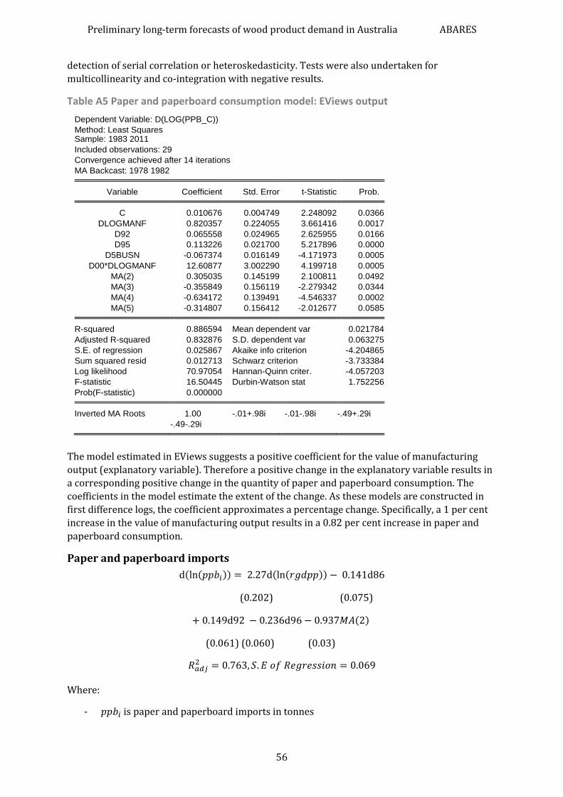
Preliminary long-term forecasts of wood product demand in Australia ABARES
56
detection of serial correlation or heteroskedasticity. Tests were also undertaken for
multicollinearity and co-integration with negative results.
Table A5 Paper and paperboard consumption model: EViews output
The model estimated in EViews suggests a positive coefficient for the value of manufacturing
output (explanatory variable). Therefore a positive change in the explanatory variable results in
a corresponding positive change in the quantity of paper and paperboard consumption. The
coefficients in the model estimate the extent of the change. As these models are constructed in
first difference logs, the coefficient approximates a percentage change. Specifically, a 1 per cent
increase in the value of manufacturing output results in a 0.82 per cent increase in paper and
paperboard consumption.
Paper and paperboard imports
(0.202) (0.075)
(0.061) (0.060) (0.03)
Where:
is paper and paperboard imports in tonnes
Dependent Variable: D(LOG(PPB_C))
Method: Least Squares
Date: 06/04/12 Time: 09:42
Sample: 1983 2011
Included observations: 29
Convergence achieved after 14 iterations
MA Backcast: 1978 1982 Variable Coefficient Std. Error t-Statistic Prob. C 0.010676 0.004749 2.248092 0.0366
DLOGMANF 0.820357 0.224055 3.661416 0.0017
D92 0.065558 0.024965 2.625955 0.0166
D95 0.113226 0.021700 5.217896 0.0000
D5BUSN -0.067374 0.016149 -4.171973 0.0005
D00*DLOGMANF 12.60877 3.002290 4.199718 0.0005
MA(2) 0.305035 0.145199 2.100811 0.0492
MA(3) -0.355849 0.156119 -2.279342 0.0344
MA(4) -0.634172 0.139491 -4.546337 0.0002
MA(5) -0.314807 0.156412 -2.012677 0.0585 R-squared 0.886594 Mean dependent var 0.021784
Adjusted R-squared 0.832876 S.D. dependent var 0.063275
S.E. of regression 0.025867 Akaike info criterion -4.204865
Sum squared resid 0.012713 Schwarz criterion -3.733384
Log likelihood 70.97054 Hannan-Quinn criter. -4.057203
F-statistic 16.50445 Durbin-Watson stat 1.752256
Prob(F-statistic) 0.000000 Inverted MA Roots 1.00 -.01+.98i -.01-.98i -.49+.29i
-.49-.29i

Preliminary long-term forecasts of wood product demand in Australia ABARES
57
is real gross domestic product per capita in 2010 AUD
, and are dummy variables for 1986, 1992 and 1996
is a moving average term.
This equation was estimated using least squares regression analysis. This method requires all
variables used in the modelling to be normally distributed and stationary. To ensure this, the
model was constructed on first differenced log data.
The purpose of the model is to establish and test the hypothesised relationship between paper
and paperboard imports and GDP per capita. Hence, specific outliers in imports were separated
to observe the effect of real GDP per capita on paper and paperboard imports. Dummy variables
for outlying import quantities in 1986, 1992 and 1996 were used. The moving average term
accounts for dynamic patterns in imports between 1983 and 2010 which are assumed to
continue to 2050.
The fitted model follows the actual data accurately and within a 95 per cent confidence interval
(Figure 12). The model was tested for stability in residuals and forecasts. It appears stable with a
high adjusted R-squared value, significant explanatory variables, consistent t-statistics and
Durbin–Watson statistic (Table A6). Further testing shows stability in the residuals with no
detection of serial correlation or heteroskedasticity. Tests were also undertaken for
multicollinearity and co-integration with negative results.
The model estimated in EViews suggests a positive coefficient for real GDP per capita. Therefore
a positive change in the explanatory variables results in a corresponding positive change in the
quantity of paper and paperboard imports. The coefficients in the model estimate the extent of
the change. As these models are constructed in first difference logs, the coefficient approximates
a percentage change. Specifically, a 1 per cent increase in real GDP results in a 2.3 per cent
increase in paper and paperboard imports.
Table A6 Paper and paperboard imports model: EViews output
Dependent Variable: D(LOG(PPBI))
Method: Least Squares
Date: 08/28/12 Time: 14:32
Sample: 1983 2010
Included observations: 28
Convergence achieved after 18 iterations
MA Backcast: 1981 1982 Variable Coefficient Std. Error t-Statistic Prob. C -0.044253 0.017084 -2.590318 0.0167
D(LOG(RGDPP)) 4.423231 0.920829 4.803532 0.0001
D86 -0.203942 0.078038 -2.613368 0.0159
D92 0.186940 0.059344 3.150087 0.0046
D96 -0.296617 0.063502 -4.670962 0.0001
MA(2) -0.973759 0.054502 -17.86636 0.0000 R-squared 0.830819 Mean dependent var 0.030261
Adjusted R-squared 0.792369 S.D. dependent var 0.140843
S.E. of regression 0.064177 Akaike info criterion -2.466920
Sum squared resid 0.090612 Schwarz criterion -2.181448
Log likelihood 40.53689 Hannan-Quinn criter. -2.379649
F-statistic 21.60769 Durbin-Watson stat 1.786133
Prob(F-statistic) 0.000000 Inverted MA Roots .99 -.99
Sample: 1983 2010
Included observations: 28
Convergence achieved after 14 iterations
MA Backcast: 1981 1982 Variable Coefficient Std. Error t-Statistic Prob. D(LOG(RGDPP)) 2.270230 0.202336 11.22009 0.0000
D86 -0.141295 0.075060 -1.882429 0.0725
D92 0.148843 0.061284 2.428753 0.0234
D96 -0.235843 0.059581 -3.958366 0.0006
MA(2) -0.937118 0.029944 -31.29588 0.0000 R-squared 0.797876 Mean dependent var 0.030261
Adjusted R-squared 0.762724 S.D. dependent var 0.140843
S.E. of regression 0.068606 Akaike info criterion -2.360437
Sum squared resid 0.108256 Schwarz criterion -2.122543
Log likelihood 38.04611 Hannan-Quinn criter. -2.287710
Durbin-Watson stat 1.807879 Inverted MA Roots .97 -.97
Preliminary long-term forecasts of wood product demand in Australia ABARES
58
Appendix B: Data assumptions In developing forecasts, the relationships between variables established through econometric
analysis of historical data are expected to continue into the future. In reality, the reliability of
forecasts will likely diminish as they extend further into the future, given the reduced reliability
of forecasts of underlying variables. This may arise because of changing relationships between
these variables, such as changes to the type of housing construction over time or growth in GDP.
This appendix lists the assumptions used to project the underlying variables used in the
econometric analysis of wood product consumption and trade.
Household size
Household size historical data were sourced from ABS social trends data. A linear trend was fit
to project household sizes which are estimated to decrease to 2.38 in 2029–30 and 2.24 in
2049–50.
Population
Population historical data were sourced from ABS census data and forecast to 2049–50 using the
growth path assumed in Strong Growth, Low Pollution (Australian Government 2011).
Population is forecast to be 29 036 783 in 2029–30 and 35 743 718 in 2049–50.
While this report uses population projections based on Australian Government (2011)
assumptions, population projections in the recently released Food demand to 2050 (Linehan et
al. 2012) ABARES report were based on the median variant of UN population projections in
2010. As the Food demand to 2050 report had a different, more global focus, UN projections were
chosen in that report for consistency when comparing modelling results with other countries.
Total dwellings
Forecasts for total dwelling commencements rely on household size, population size and a
derived estimate for total households. The number of detached and multi-dwelling
commencements was derived based on the forecast for total dwelling commencements.
We first determine the number of total households:
Where:
t represents time.
Total dwellings commenced was forecast using the following equation:
Where:
represents the total number of dwelling commencements at time t
represents the derived total number of households at time t
represents the derived total number of households at time t–1
represents a factor to account for replacement of existing housing stock.

Preliminary long-term forecasts of wood product demand in Australia ABARES
59
Historically, was calculated by re-arranging the above equation. It was then projected to
2049–50 using a six-year moving average.
The resulting forecasts for total dwellings commenced were 193 619 in 2029–30 and 214 670 in
2049–50 (Figure B1). Decreasing household sizes and an increase in population up to 2050 are
expected to increase demand for new dwellings—particularly multi-dwellings in Australia.
The ‘high’ and ‘low’ estimates for dwelling commencements are based on a +/- 5 per cent
deviation from the baseline projection for total dwellings. Comparing the forecasts for total
dwelling commencements from Love and colleagues (1999) with actual historical data for the
last decade shows an average positive error of around 4.8 per cent and an average negative
error of around 4.4 per cent. A 5 per cent deviation was thus chosen by examining these error
margins to acknowledge the potential errors and uncertainty associated with ABARES
projections for total dwelling commencements.
Figure B1 Number of total dwelling commencements, actual 1978–2011, forecasts 2012–50
Source: ABARES projections, HIA datasets
0
50
100
150
200
250
19
80
19
85
19
90
19
95
20
00
20
05
20
10
20
15
20
20
20
25
20
30
20
35
20
40
20
45
20
50
Dw
elli
ng
com
me
nce
me
nts
(in
th
ou
san
ds)
Years
High Low Base Historical

Preliminary long-term forecasts of wood product demand in Australia ABARES
60
Multi-dwellings and detached dwellings
Multi-dwelling and detached dwelling commencements were estimated as proportions of total
dwelling commencements. The ‘high’ and ‘low’ estimates are also based on the same margin for
error in ABARES projections as discussed in the assumptions for total dwellings.
Detached dwelling commencements were used for the econometric model estimating sawnwood
consumption while multi-dwellings was used in the models estimating sawnwood consumption
and imports and wood-based panel consumption and imports.
Infrastructure Australia (2010) estimated that 72 per cent of population growth occurring to
2050 will occur in capital cities. Based on this information and historical trends observed in HIA
housing data (HIA Economics 2012), the proportions of multi and detached dwellings to total
dwellings between 2011–12 and 2049–50 were estimated using a logarithmic trend. These
proportions were applied to total dwellings to derive multi and detached dwelling
commencements. In 2029–30 multi-dwelling and detached dwelling commencements are
forecast to be 79 620 and 113 999, respectively, and 102 875 and 111 795, respectively, in
2049–50 (Figure B2).
Detached and multi-dwelling commencements are forecast to rise based on the increase
required in total dwellings to meet growing population and decreasing household sizes in
Australia. While the growth in detached dwelling commencements is a marginal increase, given
the concentration of population growth in capital cities, multi-dwellings are forecast to grow at a
faster rate than detached dwellings.
Figure B2 Number of detached dwelling commencements, actual 1978–2011, forecasts 2012–50
Source: ABARES projections, HIA datasets
0
20
40
60
80
100
120
140
19
80
19
85
19
90
19
95
20
00
20
05
20
10
20
15
20
20
20
25
20
30
20
35
20
40
20
45
20
50
De
tach
ed
dw
elli
ng
com
me
nce
me
nts
(in
th
ou
san
ds)
Years
High Low Base Historical

Preliminary long-term forecasts of wood product demand in Australia ABARES
61
Figure B3 Number of multi-dwelling commencements, actual 1978–2011, forecasts 2012–50
Source: ABARES projections, HIA datasets
0
20
40
60
80
100
120
19
80
19
85
19
90
19
95
20
00
20
05
20
10
20
15
20
20
20
25
20
30
20
35
20
40
20
45
20
50
Mu
lti-
dw
elli
ng
com
me
nce
me
nts
(in
th
ou
san
ds)
Years
High Low Base Historical

Preliminary long-term forecasts of wood product demand in Australia ABARES
62
Australian to US dollar exchange rate
The Australian to US dollar exchange rate was used in the econometric model estimating
sawnwood imports. Exchange rates are considered volatile and are affected by a range of
macroeconomic indicators in Australia and in other economies. It is difficult to predict
movements in this variable. Therefore the Australian to US dollar exchange rate was projected to
2017–18 based on available information (ABARES Macroeconomic assumptions). Based on the
trend to 2017–18, the Australian to US dollar exchange rate is assumed to remain stable at
parity thereafter (Figure B4).
Figure B4 Australian to US dollar exchange rate, actual 1989–2011, forecasts 2012–50
Source: ABARES projections
Value of approved alterations and additions (renovations)
The model for wood-based panel consumption relies on forecasts for the value of approved
alterations and additions which use household size, population and a historical proportion of
renovations on existing houses.
The historical value of approved alterations and additions was sourced from the ABS and
converted to real 2004 dollars using a housing consumer price index, also sourced from the ABS.
0.00
0.20
0.40
0.60
0.80
1.00
1.20
19
90
19
95
20
00
20
05
20
10
20
15
20
20
20
25
20
30
20
35
20
40
20
45
20
50
AU
D t
o U
SD e
xch
ange
rat
e
Years
Assumed parity ABARES Macroeconomic Projection Historical
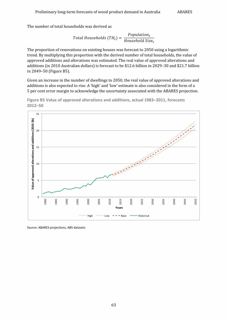
Preliminary long-term forecasts of wood product demand in Australia ABARES
63
The number of total households was derived as
The proportion of renovations on existing houses was forecast to 2050 using a logarithmic
trend. By multiplying this proportion with the derived number of total households, the value of
approved additions and alterations was estimated. The real value of approved alterations and
additions (in 2010 Australian dollars) is forecast to be $12.6 billion in 2029–30 and $21.7 billion
in 2049–50 (Figure B5).
Given an increase in the number of dwellings to 2050, the real value of approved alterations and
additions is also expected to rise. A ‘high’ and ‘low’ estimate is also considered in the form of a
5 per cent error margin to acknowledge the uncertainty associated with the ABARES projection.
Figure B5 Value of approved alterations and additions, actual 1983–2011, forecasts 2012–50
Source: ABARES projections, ABS datasets
0
5
10
15
20
25
19
80
19
85
19
90
19
95
20
00
20
05
20
10
20
15
20
20
20
25
20
30
20
35
20
40
20
45
20
50
Val
ue
of a
pp
rove
d a
lte
rati
on
s an
d a
dd
itio
ns
(201
0 $b
)
Years
High Low Base Historical

Preliminary long-term forecasts of wood product demand in Australia ABARES
64
Real gross domestic product per capita
ABS historical data was used from 1974–75 to 2009–10. Real gross domestic product was then
forecast using the growth path outlined by Global Trade and Environment Model (GTEM)
projections. GTEM is a CGE model ABARE developed to address policy issues with global
dimensions, such as international trade and is useful in projecting various macroeconomic
indicators. See Pant (2007) for a detailed description of the theoretical structure of GTEM. A per
capita estimate was derived by dividing real gross domestic product in each year with the
corresponding population forecast for that year.
Figure B6 Real gross domestic product per capita (2010 Australian dollars), actual 1983–2010, forecasts 2011–50
Source: ABS datasets, ABARES projections
0
10
20
30
40
50
60
70
80
90
19
85
19
90
19
95
20
00
20
05
20
10
20
15
20
20
20
25
20
30
20
35
20
40
20
45
20
50
Re
al g
ross
do
me
stic
pro
du
ct p
er
cap
ita
(201
0 th
ou
san
ds
AU
D)
Years
ABARES Projection Historical

Preliminary long-term forecasts of wood product demand in Australia ABARES
65
Value of manufacturing output
The proportion of value added by the manufacturing sector to real GDP was estimated
historically between 1974–75 and 2009–10. An exponential trend was then fit to estimate these
proportions out to 2049–50. This trend assumes the contribution of the manufacturing sector to
Australia’s GDP is gradually declining over time from around 8 per cent in 2009–10 to around
4 per cent in 2049–50. Manufacturing value added was then derived by applying these
proportions to the forecast for real GDP. The value added by the manufacturing sector is
estimated to increase out to 2029–30 before levelling off and declining marginally thereafter
(Figure B7).
Figure B7 Value of manufacturing output, actual 1983–2011, forecasts 2012–50
Source: ABS datasets, ABARES projections
Estimating the volume of pulplogs used domestically
Conversion factors were used to convert the volume of domestic production of paper and panels
to pulplog equivalents (Table B1). This provides an indication of the volume of pulplogs used
domestically. For pulplog harvest, calendar year data was assumed to be interchangeable with
financial year data in this report.
The volume of pulplogs harvested for domestic production of paper and panels was divided by
the volume of production of paper and panels in each year between 1997 and 2011. The
conversion factor for total paper was calculated by averaging these ratios over the 15-year
period. There appears to be a significant difference in the ratio for panels between 1997–2003
and 2004–11. Hence, the panel conversion factor was based on the average ratio between 2004
and 2011.
0
20
40
60
80
100
120
140
160
19
85
19
90
19
95
20
00
20
05
20
10
20
15
20
20
20
25
20
30
20
35
20
40
20
45
20
50
Man
ufa
ctu
rin
g va
lue
ad
de
d (
20
10
$b
)
Years
High Low Base Historical

Preliminary long-term forecasts of wood product demand in Australia ABARES
66
Similarly the volume of pulplogs harvested for woodchip exports was divided by the volume of
woodchip exports. The conversion factor for woodchip exports was calculated by averaging
these ratios over the 15-year period between 1997 and 2011.
Table B1 Conversion factors for wood products to pulplog equivalents
Type Units Conversion factor product to pulplog equivalent m3
Total paper a ’000 tonnes 1.02 Particleboard and MDF b m3 0.75 Woodchips m3 1.79
a Includes newsprint, printing and writing, household and sanitary, and packaging and industrial paper; b MDF = medium
density fibreboard.
Source: ABARES datasets
Estimating the volume of pulplogs actually harvested
Gavran and colleagues (2012) and ABARES (2012) have previously estimated the potential
volume of pulplogs available for harvest. The forecasts are based on the assumption that
harvested areas will be replanted with the same type of plantation species. The forecasts do not
take into account any future management decisions such as plantations with low growth rates
not being replanted and converted to another land use. ABARES updated these forecasts based
on anecdotal information from industry and stakeholders. As further information becomes
available, the forecasts may be revised to reflect these changes. These estimations were for
calendar year data and are assumed to be interchangeable with financial year data in this report.
To forecast the volume of woodchip exports, conversion factors were used to estimate the actual
volume of pulplogs harvested.
Parsons and colleagues (2007) and Ferguson and colleagues (2002) have previously estimated
the annual average pulplog availability from plantations in 2001–04 and 2005–09. ABARES
assumed this average annual availability to represent availability in the middle of each five-year
period. A linear trend was then used to interpolate the availability in intervening years between
each midpoint. A simple ratio of potential to actual harvest was then calculated. The conversion
factor for pulplogs harvested from hardwood and softwood plantations was calculated by
averaging these ratios over the past decade (Table B2).
Based on data from ABARES datasets, a similar ratio of availability to actual harvest was
calculated for pulplog harvest from native forests.
Table B2 Conversion factors for availability to actual pulplog harvest
Type Conversion factor Native pulplog harvest 0.95 Hardwood plantation pulplog harvest 0.68 Softwood plantation pulplog harvest 0.90
Source: ABARES datasets
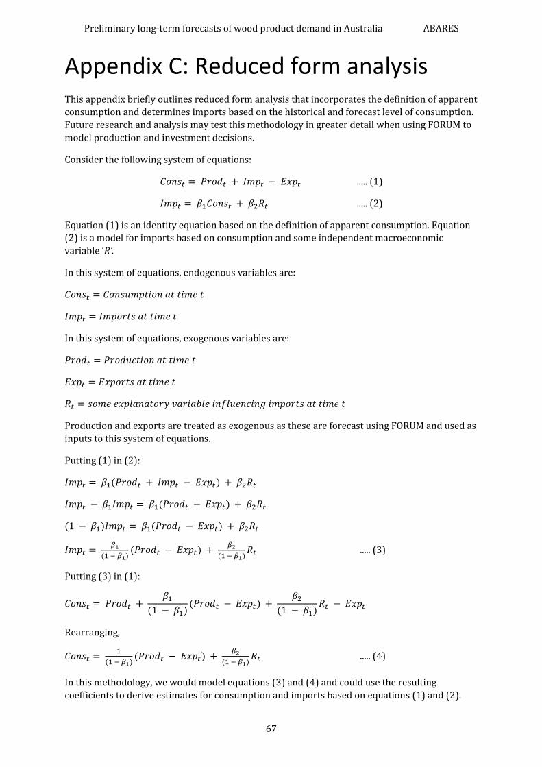
Preliminary long-term forecasts of wood product demand in Australia ABARES
67
Appendix C: Reduced form analysis This appendix briefly outlines reduced form analysis that incorporates the definition of apparent
consumption and determines imports based on the historical and forecast level of consumption.
Future research and analysis may test this methodology in greater detail when using FORUM to
model production and investment decisions.
Consider the following system of equations:
..... (1)
..... (2)
Equation (1) is an identity equation based on the definition of apparent consumption. Equation
(2) is a model for imports based on consumption and some independent macroeconomic
variable ‘R’.
In this system of equations, endogenous variables are:
In this system of equations, exogenous variables are:
Production and exports are treated as exogenous as these are forecast using FORUM and used as
inputs to this system of equations.
Putting (1) in (2):
..... (3)
Putting (3) in (1):
Rearranging,
..... (4)
In this methodology, we would model equations (3) and (4) and could use the resulting
coefficients to derive estimates for consumption and imports based on equations (1) and (2).

Preliminary long-term forecasts of wood product demand in Australia ABARES
68
References ABARES 2012, Potential effects of climate change on forests and forestry in Australia, Australian
Bureau of Agricultural and Resource Economics and Sciences, Canberra.
Australian Government 2011, Strong Growth, Low Pollution: modelling a carbon price, The
Treasury, Canberra,
archive.treasury.gov.au/carbonpricemodelling/content/chartsandtables.asp, accessed 23 May
2012.
Burke, B & Townsend, P 2011, ‘Sawnwood’, Agricultural Commodities: September quarter 2011,
Australian Bureau of Agricultural and Resource Economics and Sciences, Canberra, pp.108–113.
de Fégely, R, Blyth, M & Burns, K 2006, Scenarios for selected timber markets: summary report,
report to the Forest and Wood Products Research and Development Corporation, project no.
PN05.1021.
Edquist, A & Morris, P 1986, ‘Long term projections of the consumption of paper and paper
products in Australia’, Review of Marketing and Agricultural Economics, vol. 53, pp. 157–71.
Ferguson, I, Fox, J, Baker, T, Stackpole, D & Wild, I 2002, Plantations of Australia – Wood
Availability 2001–2044, consultant’s report for the National Forest Inventory, Bureau of Rural
Sciences, Canberra.
Gavran, M, Frakes, I, Davey, S & Mahendrarajah, S 2012, Australia’s plantation log supply 2010–
2054, Australian Bureau of Agricultural and Resource Economics and Sciences, Canberra,
adl.brs.gov.au/data/warehouse/afplsd9abfe001/afplsd9abfe00120120515/AustLogSupply201
2_2054_v.1.0.0.pdf (pdf 5.17 mb).
HIA Economics 2012, accessed May 2012,
economics.hia.com.au/media/July%202012%20%20Forecasts.pdf (pdf 173 kb).
Hossain, M, Sar, L, & Samuel, N 1989, Long term consumption projections for forest products,
ABARE Discussion Paper 89.6, Australian Bureau of Agricultural and Resource Economics,
Canberra, adl.brs.gov.au/data/warehouse/pe_abarebrs99000187/pc10112.pdf (pdf 2.44 mb).
Infrastructure Australia 2010, State of Australian Cities 2010, Canberra, March,
infrastructure.gov.au/infrastructure/mcu/soac_files/MCU_SOAC.pdf (pdf 9.90 mb), accessed
6 June 2012
Linehan, V, Thorpe, S, Andrews, N, Kim, Y & Beaini, F 2012, Food demand to 2050: Opportunities
for Australian agriculture, ABARES conference Canberra, March.
Love, G, Yainshet, A & Grist, P 1999, Forest products: long term consumption projections for
Australia, ABARE research report 99.5, Australian Bureau of Agricultural and Resource
Economics, Canberra, adl.brs.gov.au/data/warehouse/pe_abarebrs99000433/PC11465.pdf (pdf
372.76 kb).
Majumdar, S, Zhang, D & Zhang, Y 2010, ‘Estimating regional softwood lumber supply in the
United States using seemingly unrelated regression’, Forest Products Journal, vol. 60, no. 7/8, pp.
709–14, fp.auburn.edu/sfws/zhang/RefereedPub/FPJ2010–11.pdf (pdf 334.8 kb).

Preliminary long-term forecasts of wood product demand in Australia ABARES
69
Parsons, M, Frakes, I & Gavran, M 2007, Australia’s Plantation Log Supply 2005–2049, Bureau of
Rural Sciences, Department of Agriculture, Fisheries and Forestry, Canberra,
adl.brs.gov.au/data/warehouse/pe_brs90000003693/logSupply.pdf (pdf 2.75 mb).
Pant, H 2007, GTEM: Global Trade and Environment Model, ABARE Technical Report. ABARE, Canberra.
Townsend, P 2010, ‘Woodchips’, Agricultural Commodities: September quarter 2010, Australian
Bureau of Agricultural and Resource Economics and Sciences, Canberra, pp. 524–29.