Preface - isinj.com Olympiad Dark Arts - Goucher (2012).pdf · Preface In A Mathematical Olympiad...

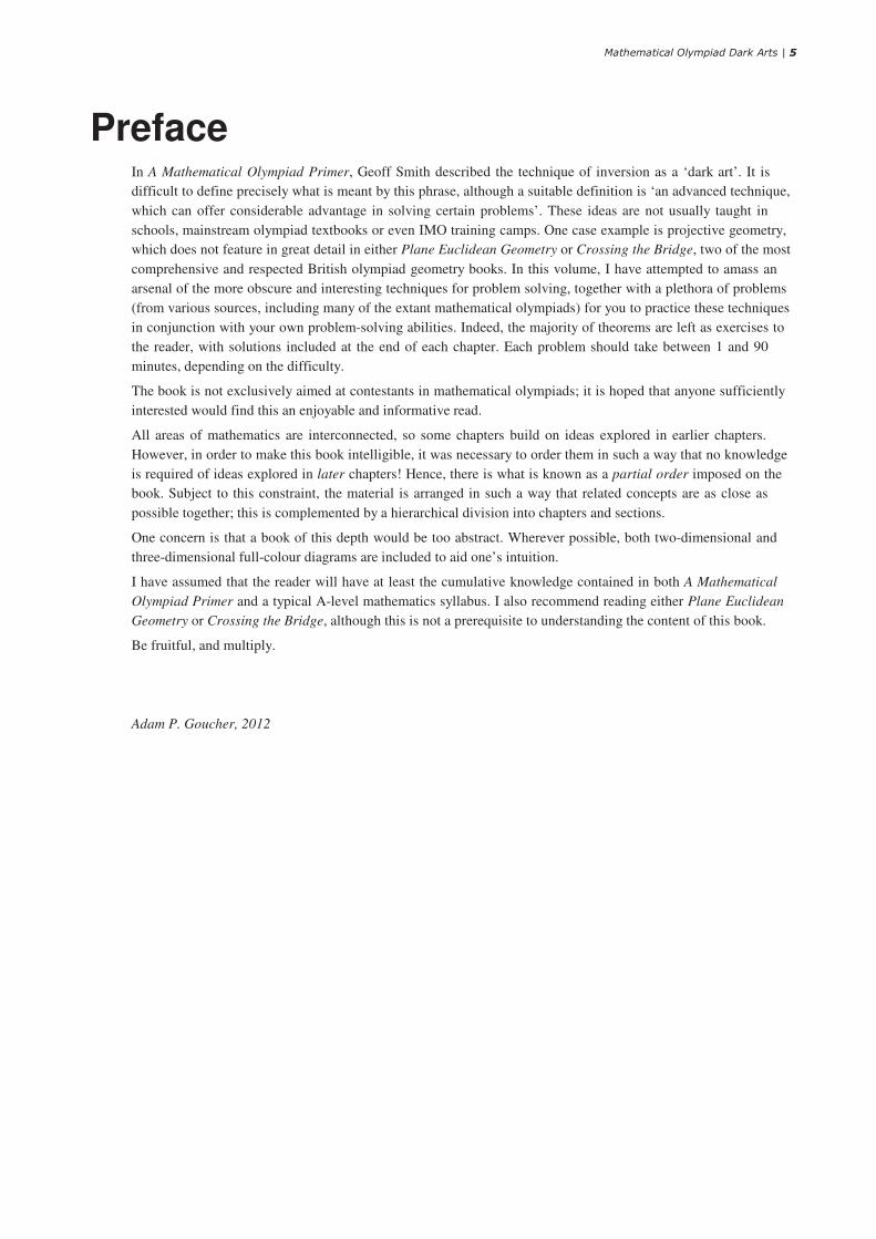
PrefaceIn A Mathematical Olympiad Primer, Geoff Smith described the technique of inversion as a ‘dark art’. It is

difficult to define precisely what is meant by this phrase, although a suitable definition is ‘an advanced technique,

which can offer considerable advantage in solving certain problems’. These ideas are not usually taught in

schools, mainstream olympiad textbooks or even IMO training camps. One case example is projective geometry,

which does not feature in great detail in either Plane Euclidean Geometry or Crossing the Bridge, two of the most

comprehensive and respected British olympiad geometry books. In this volume, I have attempted to amass an

arsenal of the more obscure and interesting techniques for problem solving, together with a plethora of problems

(from various sources, including many of the extant mathematical olympiads) for you to practice these techniques

in conjunction with your own problem-solving abilities. Indeed, the majority of theorems are left as exercises to

the reader, with solutions included at the end of each chapter. Each problem should take between 1 and 90

minutes, depending on the difficulty.

The book is not exclusively aimed at contestants in mathematical olympiads; it is hoped that anyone sufficiently

interested would find this an enjoyable and informative read.

All areas of mathematics are interconnected, so some chapters build on ideas explored in earlier chapters.

However, in order to make this book intelligible, it was necessary to order them in such a way that no knowledge

is required of ideas explored in later chapters! Hence, there is what is known as a partial order imposed on the

book. Subject to this constraint, the material is arranged in such a way that related concepts are as close as

possible together; this is complemented by a hierarchical division into chapters and sections.

One concern is that a book of this depth would be too abstract. Wherever possible, both two-dimensional and

three-dimensional full-colour diagrams are included to aid one’s intuition.

I have assumed that the reader will have at least the cumulative knowledge contained in both A Mathematical

Olympiad Primer and a typical A-level mathematics syllabus. I also recommend reading either Plane Euclidean

Geometry or Crossing the Bridge, although this is not a prerequisite to understanding the content of this book.

Be fruitful, and multiply.

Adam P. Goucher, 2012

��

Combinatorics ICombinatorics is the study of discrete objects. Combinatorial problems are usually simple to define, but can be

very difficult to solve. For example, a polyomino is a set of unit squares connected edge-to-edge, such that the

vertices are positioned at integer coordinates. The four polyominoes with three or fewer squares are shown below:

A natural question to ask is how many polyominoes there are of size n. We have already proved by exhaustion

that this sequence begins �1, 1, 2, …�. After a little effort, you will discover that there are five tetrominoes

(polyominoes of size 4) and twelve pentominoes (polyominoes of size 5). Although this is a very simple problem

to state, it is very difficult to find a formula for the number of polyominoes of a particular size. Indeed, there is no

known formula as of the time of writing, and no-one knows how many polyominoes there are of size 60. Even the

conjectured asymptotic formula, P�n� � c �n

n, is unproved (it is possible that, for instance, P�n� � c �n

n1.000001 instead).

Counting polyominoes is a hard problem. Variants of this problem are substantially easier. For instance, suppose

we restrict ourselves to polyominoes that can be created by stacking cubes in a vertical plane. To make things

even easier, we consider rotations and reflections to be distinct, so the following arrangements are counted as two

different polyominoes:

Many seemingly different combinatorial problems can be shown to be equivalent. This question can be converted

into an equivalent one by colouring the top cube in each column red, and the remainder green. We then proceed

up each column in turn, noting the colour of each cube. The configuration below is associated with the string

G R R G G R R. Every string must end in R for obvious reasons, so we may as well omit the final R and just

consider the string of n � 1 letters, G R R G G R.

��

Since each of these polyominoes has a unique string, and vice-versa, we have a bijection between the two sets.

Counting strings of a particular length is very easy (mathematicians would call this trivial); there are 2n�1 strings

of n � 1 letters chosen from �G, R�. Hence, there are 2n�1 of these restricted polyominoes. A third way of viewing

this problem is to consider it to be an ordered partition of n; the above configuration corresponds to the sum

7 � 2 � 1 � 3 � 1. So, we have solved a third combinatorial problem: there are 2n�1 ordered partitions of n identi-

cal objects into non-empty subsets.

1. How many ordered partitions are there of n into precisely k subsets?

What if we consider the partitions 2 � 1 � 3 � 1 and 3 � 1 � 1 � 2 to be equivalent? In other words, what if order

doesn’t matter? This problem can be rephrased by forcing the elements of the partition to be arranged in decreas-

ing order of size, i.e. 3 � 2 � 1 � 1. The associated diagram of this partition is known variably as a Ferrers

diagram or Young diagram.

The partition numbers are �1, 2, 3, 5, 7, 11, …�, as opposed to the ordered partition numbers

�1, 2, 4, 8, 16, 32, …�. Whereas the latter have a very simple formula, the formula for the unordered partition

numbers is given by an extremely complicated infinite series by Hardy, Ramanujan and Rademacher:

� p�n� � 1

� 2�k�1

�

k �m mod k; gcd�m,k��1

�

�

4 k�n�1

k�1

cot� � n

k cot� � n m

k �8 n m

n

sinh�

k

2

3�n� 1

24

n�1

24

Don’t be perturbed by this; the combinatorics explored in this chapter are several orders of magnitude easier than

the partition problem. We begin with the problem of colouring p beads on a necklace, where p is a prime number.

This leads to an intuitive proof of Fermat’s little theorem, and a similarly combinatorial approach yields Wilson’s

theorem. The idea of symmetry is essential, so we contemplate some group theory as well.

��

Burnside’s lemma

Consider how many ways there are of colouring the 11 beads of this necklace either red or blue. This is an

ambiguous question and there are many ways in which it can be answered:

� “There are 2048 ways of colouring the necklace.”



These answers are all valid, since the question was vague. If rotations and reflections are considered to be distinct,

then the first answer is clearly correct (as 211 � 2048). If rotations are considered to be equivalent, but reflections

are distinct, then the second is correct. The third answer applies when both rotations and reflections are equivalent.

It is easy to derive the answer 2048 in the first instance, but the others are somewhat trickier. Probably the best

way to count the number of possibilities is to use a result known as Burnside’s lemma. Firstly, we define what we

mean by a symmetry.

� A symmetry is an operation we can perform on an object. Moreover, the set of symmetries must form a group under

composition. For example, a group of rotations can be regarded as symmetries. [Definition of symmetry]

In the first case of the necklace problem, we only consider the trivial group of one symmetry: the identity. In the

second instance, we have the cyclic group of eleven symmetries (ten rotations and the identity). Finally, the third

case requires the dihedral group of twenty-two symmetries (eleven reflections, ten rotations and the identity).

R

A direct symmetry can be expressed as a sequence of rigid transformations, such as translations and rotations. For

example, the red and blue Rs are related by a direct symmetry (rotation by � through their common barycentre),

By comparison, the green R cannot be obtained from the red R by a sequence of rotations and translations, so is

related to the red R by an indirect symmetry (in this case, a reflection). The composition of two direct or two

indirect transformations is a direct transformation; the composition of a direct and indirect transformation is an

indirect transformation. This idea can be succinctly represented as a 2�2 Cayley table:

� D I

D D I

I I D

� An object is said to be fixed by a symmetry if it is unchanged by applying that symmetry. [Definition of ‘fixed’]

��

For example, the hyperbola x2 � y2 � 1 is fixed by a rotation of � about the origin, whereas the parabola y � x2 is

not.

� The number of distinct objects is equal to the mean number of objects fixed by each symmetry. [Burnside’s lemma]

For the second case of the necklace problem, there are 11 symmetries. The identity symmetry fixes all 2048

objects, whereas the ten rotations only fix two objects (the monochromatic necklaces). So, Burnside’s lemma

gives us a total of 1

11�2048 � 10�2� � 188 unique necklaces. Similarly, for the third case, we observe that there

must be 26 � 64 objects fixed by each of the 11 reflections, so we have 1

22�2048 � 10�2 � 11�64� � 126 unique

necklaces. That this gives an integer answer is a useful way to check your arithmetic.

The cube has a group of 24 direct symmetries (and the same number of indirect symmetries). We can classify

those 24 direct symmetries into five conjugacy classes:

� 1 identity symmetry;

� 6 rotations by 1

2� about the blue axes;

� 3 rotations by � about the blue axes;

� 6 rotations by � about the red axes;

� 8 rotations by 2

3� about the green axes.

2. Suppose we colour each face of a cube one of k colours. By considering the number of colourings fixed by

each of the above symmetries, deduce the number of distinct colourings of the cube where rotations are

considered equivalent.

Fermat’s little theorem

��

We now generalise the previous question to a necklace of p beads (where p is prime) and c different colours.

3. How many distinct ways can a necklace of p beads be coloured with c colours, where p is prime and c � 2?

Rotations are considered to be equivalent, whereas reflections are distinct.

4. Hence show that cp c �mod p�. [Fermat’s little theorem]

Fermat’s little theorem only applies when the modulus is prime. If, instead, the modulus is composite, it is

necessary to use a generalisation by Euler. Unlike Fermat’s little theorem, Euler’s generalisation does not appear

to be a consequence of applying Burnside’s lemma to necklaces of n beads.

� If a and n are coprime, then a��n� 1 �mod n�, where ��n� is Euler’s totient function (the number of positive integers

k � n which are coprime to n). [Euler-Fermat]

Euler’s totient function can easily be computed when the prime factorisation of n is known. Specifically, we have

the rule ��a b� � ��a� ��b� if a and b are coprime, and ��pn� � �p � 1� pn�1.

Suppose N � p q is a product of two distinct primes, each of which has hundreds of digits. Given N, there is no

known algorithm capable of factorising it to find p and q in a reasonable (polynomial) amount of time. This can

be used as the basis of a cryptographic system known as RSA (after its creators, Rivest, Shamir and Adleman).

The idea is that we define a function, f : �N ��N , which the general public has access to. However, we keep the

inverse function f �1 secret.

5. Suppose that b � f �a� ad �mod N�. Show that f �1�b� be �mod N�, where d e 1 �mod ��N��. [Basis of

RSA]

In other words, we publish a, d, N (and therefore f ) but leave p, q, e secret. As it is impossible to compute e

from d without knowledge of p and q, the general public cannot calculate f �1. Hence, they can encrypt an integer,

but not decrypt it. As the numbers in �N can have hundreds of digits, it is possible to store a substantial amount

of information in one integer. This is typically used to encrypt passwords, safe in the knowledge that there is no

known algorithm for rapidly factorising semiprimes.

Interestingly, there is an algorithm called AKS which enables a computer (or, more correctly, Turing machine) to

determine whether a number is prime in polynomial time (in the number of digits), but actually factorising the

number may require exponential time. Additionally, so-called ‘quantum computers’ are capable of prime factorisa-

tion in cubic time, so a sufficiently powerful quantum computer would render RSA useless. Fortunately, this

technology is a long way off, and the largest semiprime factorised by Shor’s algorithm as of the time of writing is

15 � 5�3 using a machine with seven quantum bits.

��

Wilson’s Theorem

RR

RR

RR

RR

RR

RSuppose we have a p� p chessboard, where p is prime. We label each square with a coordinate �x, y�, where x

and y are considered modulo p (in effect, forming a toroidal surface). We then place an arrangement of p non-

attacking rooks on the chessboard, i.e. one in every row and one in every column. We consider the group of p2

symmetries (one identity and p2 � 1 translations).

6. Show that there are p � arrangements fixed by the identity symmetry.

7. Show that no arrangements are fixed by any of the 2 �p � 1� horizontal or vertical translations.

8. Show that p arrangements are fixed by each of the �p � 1�2 remaining translations.

9. Hence determine the number of unique arrangements, where toroidal translations of the board are

considered equivalent.

10. Prove that �p � 1�� 1 modulo p if p is prime. [Wilson’s theorem]

If n is composite, then �n � 1�� 0 modulo n, except where n � 4, in which case �n � 1�� 2. Hence, the converse

of Wilson’s theorem is also true.

Packings, coverings and tilings

Straddling the boundary between combinatorics and geometry is the idea of tessellations, or tilings.

Consider a set S of [closed] tiles, each of which is a subset of some region R. If the pairwise intersection of any

two tiles of S has zero area, then S is a packing. If the union of all tiles in S is the entirety of R, then S is a cover-

ing. If both of these conditions hold, it is a tiling.

The diagram above highlights the differences. The first diagram is a packing using two blue circles. The second is

��

a covering using four red circles. The third diagram is both a packing and covering, and thus a tiling, using four

green isosceles right-angled triangles.

Using circles of unit radius, there are obviously no tilings of the plane. It is of interest to find the packing of the

highest density and covering of the lowest density.

It has been proved that the optimal packings and coverings of the plane using circles of unit radius are obtained by

positioning them at the vertices of the regular triangular tiling. Other optimisation problems are solved by the

hexagonal lattice, which is why honeybees favour hexagonal honeycombs as opposed to a rectangular Cartesian

grid. In higher dimensions, less is known. For three dimensions, the optimal lattice packing of spheres is the face-

centred cubic lattice A3 � �x, y, z� ��3, x � y � z 0 �mod 2��, whereas the optimal lattice covering is the body-

centred cubic lattice A3� � �x, y, z� ��3, x y z �mod 2��.

Each sphere in the face-centred cubic packing is adjacent to twelve other spheres. This suggests another packing

problem: what is the maximum number of disjoint unit spheres tangent to a given unit sphere? In two dimensions,

the answer is rather trivially six. In three dimensions, Isaac Newton conjectured that the maximum is indeed

twelve spheres, whereas David Gregory hypothesised that thirteen could be achieved. It transpires that Newton

was correct. The problem has also been solved in 4, 8 and 24 dimensions, again corresponding to the arrange-

ments of spheres in very regular lattice packings (known as D4, E8 and �24, respectively). �24 (the Leech lattice)

has so many interesting properties and profound connections that I cannot hope to list them all here. Nevertheless,

its existence is related to string theory, error-correcting codes, the Monster group, and the curious fact that

12 � 22 � 32 � … � 242 � 702.

Colouring arguments

To begin with, we ponder tilings of finite, discrete spaces. For example, consider a standard 8�8 chessboard with

two opposite corners removed. Is it possible to tile the resulting shape with 31 1�2 dominoes?

��

If the chessboard is coloured as above, each domino must occupy precisely one blue and one red square. As there

are 32 blue and 30 red squares, it is clearly impossible to tile it with 31 dominoes.

The more general problem of determining whether a polyomino-shaped region can be tiled with dominoes can be

embedded in graph theory. We represent the squares with vertices, and join vertices corresponding to adjacent

squares. Some regions clearly cannot be tiled, even if they have equal quantities of squares of each parity. One

such example is the following ‘octomino’, shown below with an equivalent bipartite graph:

The lowest blue vertex in the graph is connected to three red vertices, two of which are exclusively connected to

this blue vertex. It is therefore impossible to place disjoint dominoes to cover both of the corresponding red

squares. However, the basic colour-counting argument is insufficient here, as there are four red and four blue

squares.

In effect, we want to find a bipartite matching between the red and blue vertices of the graph. A necessary and

sufficient condition for there to exist an injection from the red vertices to the blue vertices is Hall’s marriage

theorem.

� Let S be the set of red vertices, and T be the set of blue vertices. Consider each subset S ' � S, and let T ' � T be the set

of vertices directly connected to vertices in S '. Then there exists an injection from the red vertices to the blue vertices

if and only if S ' � T ' for all subsets S '. [Hall’s marriage theorem]

For a bijection, it is necessary and sufficient that there are equal numbers of red and blue vertices and the above

result also holds. Returning to the octomino problem, note that the two red vertices of degree 1 are connected to

the same blue vertex, so the marriage condition does not hold.

Verifying the marriage condition can be a time-consuming process, as there are 2n subsets of red vertices for a

bipartite graph with n red and n blue vertices. This is faster than checking every possible bijection, of which there

are n �. Both of these algorithms are said to take exponential time. People are interested in fast, polynomial-time

algorithms, as they usually can be executed in a reasonable amount of time.

Colouring can solve much more general problems than the domino tiling problem.

11. Determine whether it is possible to tile a 4�7 rectangle with (rotations of) each of the seven tetrominoes

(where reflections are considered to be distinct). The seven tetrominoes are shown below:

��

12. Is it possible to tile a 6�6 rectangle with 15 dominoes and 6 non-attacking rooks? [Ed Pegg Jr, 2002]

13. Show that the maximum number of (grid-aligned) k�k square tiles that can be packed into a m�n

chessboard is given by �m

k � n

k .

In addition to determining whether or not a region can be tiled, it is occasionally possible to enumerate precisely

how many ways in which this can be done. This is typically accomplished using recursion on the size of the

region.

14. In how many ways can a 2�n rectangle be tiled with n dominoes?

This is a simple case of what one would initially imagine to be a completely intractable problem: to count the

number of domino tilings of a m�n rectangle. A remarkable discovery by Kasteleyn enumerates this for any

planar graph, and thus how many domino tilings exist for any polyomino. In particular, a m�n chessboard can be

tiled by dominoes in exactly �k�1

n

�l�1

m

4 cos2 � l

m�1� 4 cos2 � k

n�14 ways.

Regular solids and tilings

Suppose we attempt to tile a surface with regular n-gons, where k n-gons meet at each vertex. To avoid trivial

cases, we assume that both k and n exceed 2. The cases where the Schläfli symbol �n, k� is either �3, 3�, �4, 3�,�3, 4�, �5, 3� and �3, 5� result in the five regular solids, namely the tetrahedron, cube, octahedron, dodecahedron

and icosahedron.

They are also referred to as Platonic solids, as Plato believed that all matter was composed (at the atomic level) of

minuscule cubes, tetrahedra, octahedra and icosahedra, associating each one with a different classical element. He

reserved the dodecahedron for representing the entire universe.

15. Each face of a regular dodecahedron is infected with either E. coli, S. aureus or T. rychlik bacteria. In how

many ways is this possible, treating rotations as equivalent? [Adapted from Google Labs Aptitude Test]

If �n, k� is �6, 3�, �4, 4� or �3, 6�, we obtain the hexagonal, square and triangular tilings, respectively, of the plane.

The Platonic solids can be regarded as analogous tilings of the sphere.

��

If �n, k� is anything other than these eight possibilities, the sum of the angles around each vertex exceeds 2 �. This

is only possible in the bizarre hyperbolic surfaces described by Bolyai-Lobachevskian geometry.

On the complex plane, numbers of the form a � b (a, b ��) form a ring known as the Gaussian integers, which

are positioned at the vertices of the square tiling. As Euclid’s algorithm can be applied to the Gaussian integers,

the fundamental theorem of arithmetic still holds: Gaussian integers can be factorised uniquely into a product of

Gaussian primes (up to multiplication by the units, 1, �1, and �). Not all ordinary primes are Gaussian primes;

for example, 2 is not a Gaussian prime, as it can be factorised as �1 � � �1 � �.Suppose we have a grasshopper initially positioned at the origin, which can only jump to a Gaussian prime within

the disc of radius R centred on its current position. It is an unsolved problem as to whether there is some R for

which the grasshopper can visit infinitely many Gaussian primes.

�3 �2 �1 1 2 3

�3

�2

�1

1

2

3

�3 �2 �1 1 2 3

�3

�2

�1

1

2

3

Similarly, numbers of the form a � b � (a, b ��), where � is a primitive cube root of unity, form the ring of

Eisenstein integers. They are positioned at the vertices of the triangular tiling. As with the Gaussian integers, the

fundamental theorem of arithmetic applies. The units are the sixth roots of unity, namely �1, ��, ��2�. It ispossible to find the squared distance between two Eisenstein integers a and b by expressing the vector a � b in

��

terms of 1, �, �2� and calculating a � b 2 � �a � b� �a� � b��, remembering that 1 � � ��2 � 0 and �3 � 1.

16. A set S of 99 points are drawn in the plane, such that no two are within a distance of 2 units. Prove that

there exists some subset T � S of 15 points, such that no two are within a distance of 7 units.

Aperiodic tilings

As we noted, the only regular polygons capable of tiling the Euclidean plane are the triangle, square and hexagon.

Pentagons cannot, as three pentagons at each vertex have an interior angle sum of 9

5�, which is slightly less than

2 � and causes the pentagons to ‘curl up’ into a dodecahedron. Similarly, attempting to place four or more pen-

tagons around each vertex results in a hyperbolic tiling, as 12

5� � 2 �.

More strongly, there is no tiling of the plane which exhibits both translational symmetry and order-5 rotational

symmetry. To prove this, we assume without loss of generality that the tiling is fixed by both a translation parallel

to the vector 1

0 and a rotation by

2

5� about the origin. In that case, it is possible to map the origin to any point

expressible as the sum of fifth roots of unity.

�3 �2 �1 1 2 3

�3

�2

�1

1

2

3

The points on the real axis expressible in this way are those of the form a � b �, where a, b �� and

� �1

2�1 � 5 . As � is an irrational number, these points form a dense subset of the reals, i.e. for every � � 0,

every point x on the real axis is within a distance of � from a point of the form a � b �. This means that the tiling

must be composed of infinitesimally small tiles, which contradicts our notion of discrete tiles.

��

If we dispose of the translational symmetry, we can indeed have tilings with order-5 rotational symmetry. Perhaps

the most famous is an aperiodic tiling known as the Penrose tiling (above), formed from interlocking ‘thin’ and

‘thick’ rhombi in the ratio 1 : �. It is a remarkable fact that every tiling of the plane with these two tiles (and

certain matching rules) exhibits this ratio, and is thus aperiodic (since � is irrational). An unsolved problem is

whether there is a single connected shape (an ‘aperiodic monotile’), which can only tile the plane aperiodically.

Joshua Socolar and Joan Taylor recently (2010) discovered a disconnected aperiodic monotile based on the

hexagonal honeycomb, suggesting that there may indeed be a connected variant waiting to be found.

There is a three-dimensional analogue of the Penrose tiling. It is formed from equilateral parallelepipeds (three-

dimensional rhombi) and displays icosahedral symmetry. Crystallographers were very surprised to find naturally

occurring crystals with this structure, termed ‘quasicrystals’. It was previously believed that solids could only be

either periodic crystals or totally irregular.

Invariants

An invariant is, as suggested by the name, something that doesn’t change. One of the simplest invariants is parity:

whether something is even or odd. Integers are one of the most common things to display parity; however, the

idea is equally applicable to other things such as permutations. To realise that permutations have a parity, it is

necessary to consider them in a more geometrical light.

An n-simplex is a regular n-dimensional figure (polytope) with n � 1 vertices, which is fixed under any permuta-

tion of the vertices. The 1-simplex, 2-simplex and 3-simplex are the line segment, triangle and tetrahedron,

respectively, as in the above diagram. Interchanging two of the vertices of a simplex can be regarded as a reflec-

tion. For example, reflecting a regular tetrahedron A B C D with circumcentre O in the plane O C D causes the

vertices A and B to be swapped.

��

This suggests two different sets of permutations: the odd permutations, which correspond to indirect isometries of

�n; and even permutations, which correspond to direct isometries. A k-cycle (cyclic permutation of some subset

containing k elements) is an odd permutation if k is even, and vice-versa. In particular, 2-cycles (or swaps) are

odd permutations.

The set of even permutations of n elements forms a group known as the alternating group An. This is a subgroup

of the group of all permutations, known as the symmetric group Sn. Any composition of even permutations is

itself an even permutation, which can form a useful invariant. For example, it shows that not all conceivable

configurations of a Rubik’s cube can be attained by applying legal moves to the initial ‘solved’ position.

17. Suppose we have a hollow 4�4 square containing 15 unit square tiles and one empty space, into which any

adjacent tile can be moved. The fifteen tiles are numbered from 1 to 15. Determine whether it is possible to

get from the left-hand configuration to the right-hand configuration in the diagram below. [Sam Loyd’s 15

puzzle]

1 2 3 4

5 6 7 8

9 10 11 12

13 14 15

?

1 2 3 4

5 6 7 8

9 10 11 12

13 15 14

Instead of an invariant, it is possible to define a value that only changes in one direction, known as a monovariant.

This is useful for proving that a process (such as a perturbation argument) eventually terminates.

18. There are n red points and n blue points in the plane, no three of which are collinear. Prove that it is

possible to pair each red point with a distinct blue point using n non-intersecting line segments. [EGMO

2012, Friday bulletin]

Solitaire

Quite a few interesting problems pertain to the game of peg solitaire. We have a (possibly infinite) board, which is

a subset of �2 containing some (possibly infinite) initial configuration of identical counters. The only allowed

move is to jump horizontally or vertically over an occupied square to an unoccupied one; the piece that has been

jumped over is removed. This is demonstrated below.

19. Suppose we have a game of solitaire on a bounded board beginning with the configuration of 32 pieces

shown below. Show that if we can reach a position where only one piece remains on the board, then we can

do so where the piece is in the centre.

��

20. We begin with an infinite chessboard, and divide the board into two half-planes with a straight horizontal

line. All squares below the line are occupied with counters; all squares above the line are unoccupied. Show

that it is impossible, after a finite sequence of moves, for a counter to occupy the fifth row above the line.

[Conway’s soldiers]

21. Suppose we have an infinite chessboard with an initial configuration of n2 pieces occupying n2 squares that

form a square of side length n. For what positive integers n can the game end with only one piece remaining

on the board? [IMO 1993, Question 3]

��

Solutions

1. We are enumerating strings containing precisely k � 1 Rs and n � k Gs. Hence, the number of ordered

partitions of n into k subsets is given by the binomial coefficient n � 1

k � 1�

�n�1��k�1�� n�k�� .

2. All k6 colourings of the cube are fixed by the identity. Consider a rotation by 1

2� about the vertical blue

axis. The top and bottom faces can be any colour, whereas the four other faces must all be the same colour.

Hence, each of the 6 symmetries in this conjugacy class fix k3 colourings. By similar reasoning, the 3

rotations by � about the blue axes each fix k4 colourings. The 6 rotations about the red axes each fix k3

colourings, whereas the 8 rotations by 2

3� about the green axes fix only k2 colourings. Applying Burnside’s

lemma, the total number is 1

24�k6 � 3 k4 � 12 k3 � 8 k2�.

3. There are p symmetries, namely the identity and p � 1 rotations. The former fixes all np colourings,

whereas the latter fixes only the n monochromatic necklaces. Hence, we have 1

p�np � n�p � 1�� unique

necklaces.

4. The result of the previous question is an integer, so cp � c�p � 1� is divisible by p. Hence, cp � c p � c 0.

As c p 0, this means that cp c �mod p�.

5. Note that ��N� � ��p� ��q� � �p � 1� �q � 1�. Expressing b in terms of a, we obtain be � ad e. As

a��N� 1 �mod N� by Euler-Fermat, and d e 1 �mod ��N��, ad e a1 � a �mod N�, so is precisely the inverse

function we are looking for.

6. The position of the rooks can be regarded as a bijection mapping rows to columns. There are p � permutations of p elements.

7. Without loss of generality, just consider horizontal translations by �a, 0�. If there is a rook in �x, y�, there

must also be a rook in �x � a, y�, contradicting the assumption that the rooks are non-attacking.

8. Consider the rook positioned at the coordinates �x, 0�, and let the translation be parallel to vector �a, b�. This forces there to be rooks in positions �x � a, b�, �x � 2 a, 2 b�, …, �x � a, �b�. Hence, the arrangement is

determined uniquely by the abscissa of the rook in the 0th row, of which there are p possibilities. Hence, p

arrangements are fixed by each of these translations.

9. We have 1

p2�p � � p�p � 1�2� distinct arrangements by Burnside’s lemma.

10. The previous answer must be an integer, so p � � p�p � 1�2 0 �mod p2�. Dividing throughout by p, we

obtain �p � 1�� p � 1�2 0 �mod p�. We can expand this to yield �p � 1� � � p2 � 2 p � 1 0 �mod p�. As

p2 and 2 p are divisible by p, we can eliminate those terms, resulting in the statement of Wilson’s theorem.

11. Colour the squares black and white, as on a standard chessboard. The T-shaped tetromino must cover three

black squares and one white square (or vice-versa), whereas each of the other tetrominoes cover precisely

two squares of each colour. As the chessboard features equal numbers of black and white squares, this is

indeed impossible.

12. Colour the squares black and white, as on a standard chessboard. The six rooks are positioned on squares

�i, ��i��, where � is a permutation of �1, 2, 3, 4, 5, 6�. Select two rooks at positions �i, ��i�� and � j, �� j��, and move them to �i, �� j�� and � j, ��i��, respectively. Applying this move does not alter the parity of rooks

on white squares. Since we can do this until they lie on the long diagonal of white squares, it is clear that

��

there must have been an even number of rooks on white squares to begin with. However, the constraint that

the remaining 30 squares can be tiled by dominoes forces the rooks to occupy three white and three black

squares, which contradicts the previous statement. Hence, it is impossible.

13. Represent each square with coordinates �x, y�, where x � �1, 2, …, m� and y � �1, 2, …, n�. Colour the

square blue if x y 0 �mod k�, and white otherwise. Clearly, each tile must conceal precisely one blue

square, and there are only �m

k � n

k of them. This bound is attainable.

14. Let this number be denoted f �n�. Either the rightmost 2�1 rectangle is a (vertical) domino or the rightmost

2�2 rectangle is a pair of horizontal dominoes. Now consider how many ways there are of tiling the

remaining area. In the first case, there are f �n � 1� possible configurations; in the second, there are f �n � 2�. This gives us the recurrence relation f �n� � f �n � 1� � f �n � 2�. Together with the obvious fact that

f �1� � 1 and f �2� � 2, this generates the Fibonacci sequence, f �n� � F�n � 1�.

15. There are 60 symmetries of the regular dodecahedron. The identity symmetry fixes all 312 infections. There

are 24 rotations about axes passing through the centres of opposite faces, each of which fix 34 infections.

The 15 rotations about axes passing through the midpoints of edges each fix 36 infections. Finally, the 20

rotations about axes passing through opposite vertices each fix 34 infections. By Burnside’s lemma, there

are 1

60�312 � 24�34 � 15�36 � 20�34� � 9099 unique infections of the dodecahedron with three strains of

bacteria.

16. Tile the plane with the regular hexagonal tiling, where each hexagon has side length 1. Clearly, no two

points in S can occupy the same hexagon. 7-colour the hexagons in a repetitive fashion, such that each

hexagon is adjacent to six hexagons of different colours. By the pigeonhole principle, at least 15 of the

points must lie in identically-coloured hexagons. It is straightforward to show that no two of those points

can be within 7 of each other, by considering the closest approach of the vertices of the hexagons and

using cube roots of unity to calculate the distance: the arrow shown in the honeycomb below has a complex

vector of 2 � �, which has squared length �2 � �� 2 � �2�� 4 � 2 �� 2� � 1 � 7.

��

17. Label the empty space with 0, so we can regard this as a permutation of �0, 1, …, 15�. Consider the parity of

x � y, where �x, y� is the location of the empty space, together with the parity of the permutation �. Note

that each move flips both parities, thus leaving the total parity of x � y � � unchanged. However,

interchanging any two tiles without moving the empty space alters the parity of x � y � �, so it is impossible

to get from the left configuration to the right configuration.

18. Biject them in an arbitrary way using n line segments. If we encounter a configuration of four points joined

by two intersecting line segments, as above, then we can replace the line segments with disjoint line

segments. Let the monovariant E be the total length of line segments. E strictly decreases at each step (by

the triangle inequality), so the process cannot cycle. As there are only finitely many bijections between red

and blue points, the process must terminate with n disjoint line segments.

��

19. Firstly, colour the tile at coordinates �x, y� either red, green or yellow depending on the value of x � y

modulo 3, where we consider the central tile to be the origin (coloured red). As the parities of red, green and

yellow counters all change simultaneously when a solitaire move is played, the final counter must be on a

red square. However, we can also colour the tiles depending on x � y modulo 3, resulting in a perpendicular

pattern of colouring as shown above. The only tiles that are red in both colourings are given by �3 i, 3 j�, where i and j are integers. On the bounded board, there are only five such tiles. Backtracking by one move

must result in a configuration equivalent to the one shown below, in which case we can trivially jump to the

central square.

20. Assume that it is possible to reach a square in the fifth row, in attempt to derive a contradiction. Without

loss of generality, we will use T � �0, 0� as the ‘target square’. For each square �x, y�, we assign a value of

�� x � y �, where x � y is the Manhattan distance between �x, y� and �0, 0�, and � �1� 5

2 is the golden

ratio. Let E be the sum of the values of the occupied squares. If a counter on a square of value �k jumps

over one of value �k�1, this results in a single counter on a square of value less than or equal to �k�2. As

�k�2 � �k�1 � �k, the value of E cannot increase. At the beginning of the game, the value of E can be

calculated by summing some geometric progressions; it is simple to show that this value equals 1. As the

value of the target square is also 1, it is necessary to use all of the counters to reach it. However, that is

impossible in a finite amount of time, as there are infinitely many counters.

21. For n � 1 and n � 2, this is trivial. If we have an arrangement shown above, it is possible to ‘delete’ three

adjacent pieces. This can be used, rather effectively, to reduce a problem from n � 3 k � 4 to n � 3 k � 2 by

��

deleting the outermost ‘layer’ of pieces, as in the diagram below. Similarly, we can reduce a problem from

n � 3 k � 5 to n � 3 k � 1 by deleting the outermost two layers. By induction, we can solve the problem for

all n except for multiples of three. If n is a multiple of three, we colour the tile at coordinates �x, y� either

red, green or yellow depending on the value of x � y modulo 3. Let the number of pieces on red, green and

yellow tiles be indicated by R, G and Y , respectively. Note that if ��1�R � ��1�G � ��1�Y before a solitaire

move, then it will remain true afterwards. This condition is clearly true for a 3 k�3 k square of pieces, but

false for a single piece. Hence, we cannot reduce the arrangement to a single piece if n is a multiple of 3.

��

Linear algebraThe second chapter of this book is concerned with vectors, matrices and linear transformations. Determinants are

introduced, together with ways in which to calculate them. These concepts are particularly relevant in analytic

geometry, where we use them to describe projective transformations.

Linear transformations

Linear transformations are transformations of n-dimensional Euclidean space �n expressible as x � M x, where

x � �x1, x2, …, xn� is the position vector of a point X . M is known as the transformation matrix. For example, the

linear transformation with matrix 1 1

0 1 is shown below.

O

The position of the origin, O, is left unchanged by a linear transformation. Degree-d algebraic curves remain as

degree-d algebraic curves; in particular, lines map to lines and conics map to conics. In the shear shown above, a

circle is transformed into an ellipse. Parallel lines remain parallel when linear transformations are applied.

Finally, the (signed) area of any shape is multiplied by det�M � when the transformation is applied, where det�M �is the determinant of the transformation matrix. Hence, ratios of areas remain unchanged.

Common linear transformations include rotations (about the origin), reflections (in lines through the origin),

dilations (where the origin is the centre of homothety) and stretches (again, preserving the origin). One can

combine transformations by multiplying their matrices.

1. Let A � �1, 0, 0�, B� �0, 1, 0� and C � �0, 0, 1� be three points in �3. After applying the transformation with

matrix M �

a b c

d e f

g h i

, find the new locations of A, B and C.

Consider the unit cube �0, 1�� 0, 1��0, 1�, where � denotes Cartesian product. It is transformed into a paral-

lelepiped with volume V � det�M �.

In the diagram above, the blue cube is transformed into the red parallelepiped. The origin (the common vertex of

the cube and parallelepiped) remains fixed.

��

Determinants

The determinant of a square matrix M is a positive real number det�M � associated with that matrix. It behaves

like the norm of a complex number, in that it is multiplicative.

� For two square matrices A and B of equal dimension, det�A B� � det�A� det�B�. [Multiplicativity of determinants]

If a matrix A has an inverse matrix A�1 such that A A�1 � A�1 A � I , then det�A� det�A�1�� det�I� � 1. Hence, it is

clear that a matrix with a determinant of zero has no inverse. Indeed, the converse is also true: all square matrices

with non-zero determinants possess unique well-defined inverses. If a matrix is one-dimensional, then its

determinant is equal to its only element. Otherwise, we compute it recursively.

M �

a1,1 a1,2 � a1,n

a2,1 a2,2 � a2,n

� � � �

an,1 an,2 � an,n

Consider the matrix above. We compute the determinant using the following process:

� For some 1 � i � n, consider the element ai,1 in the first column of M .

� The �n � 1�-dimensional matrix Mi is obtained by removing everything in the same row or column as ai,1.

� Compute the value Si � ai,1 det�Mi�.

� Then, we have det�M � � S1 � S2 � S3 � S4 � … � ��1�n�1 Sn.

This recursion results in the determinant equating to a sum of n � terms, each of which is a product of n elements

of M . After expanding this somewhat complicated recursive definition, we reach a more elegant formulation.

� det�M � � �sym

��1�P�� a1,��1� a2,��2� … an,��n��, where the sum is taken over all permutations � of �1, 2, 3, …, n�. We

define P�� to be even if � is an even permutation, and odd otherwise. [Leibniz formula for determinants]

2. Express det

x y z

z x y

y z x

as a polynomial in x, y, z.

You may have noticed that for 3�3 determinants, the even permutations correspond to the three NW-SE

‘diagonals’ and the odd permutations correspond to the three NE-SW ‘diagonals’. The diagonals are considered to

wrap around the edges of the matrix as though it were a cylinder. This trick is known as the Rule of Sarrus.

a

d

g

b

e

h

c

f

i

a

d

g

b

e

h

c

f

i

a e i� b f g � c d h �a f h� b d i� c e g

Leibniz’s formula requires n�n �� elementary operations, so is rather time-consuming for large matrices, taking

exponential time. Instead, it helps to simplify the calculation by performing operations on the matrix.

��

� Applying elementary operations to the rows or columns of M cause its determinant to behave in a predictable manner:

� Multiplying any row or column of M by x causes the determinant of M to be multiplied by x;

� Adding (or subtracting) any multiple of one row to another row does not affect the determinant of M ;

� Swapping any two rows causes det�M � to be multiplied by �1;

� The transpose of M has the same determinant as M .

This can also be used to easily factorise the determinants of matrices.

3. Factorise det

1 1 1

x y z

x3 y3 z3

into four linear factors.

Interpolating curves

The determinant of a matrix is zero if and only if one row can be expressed as a linear combination of the others.

This is known as linear dependence. This enables one to create a curve of some type (e.g. a polynomial, circle or

conic) interpolating between various points. For example, if we have a sequence of n points �xi, yi�, then the

following curve is a degree-�n � 1� polynomial passing through all n points.

� The curve det

1 y x x2 x3 � xn�1

1 y1 x1 x12 x1

3 � x1n�1

� � � � � � �

1 yn xn xn2 xn

3 � xnn�1

� 0 passes through all points �xi, yi�. [Lagrange interpolating

polynomial]

This is obvious, as the determinant equals zero if two rows are identical. It is also a degree-�n � 1� polynomial, as

we can use the recursive determinant formula to express it as A1 � A2 y � A3 x � A4 x2 � A5 x3 � … � An�1 xn�1

and rearrange it. If A2 � 0 then this method will fail, but that only occurs if two points have the same abscissa.

Using this idea, we can create a unique conic passing through any 5 points in general position, a cubic passing

through 9 points et cetera. If the points are not in general position, then seemingly paradoxical things can occur.

This forms the basis of the powerful Cayley-Bacharach theorem explored in the projective geometry chapter. The

general equation of a conic is A � B x � C y � D x2 � E y2 � F x y � 0, so we can determine the equation of the

conic passing through five given points.

� The conic

1 x y x2 y2 x y

1 x1 y1 x12 y1

2 x1 y1

1 x2 y2 x22 y2

2 x2 y2

1 x3 y3 x32 y3

2 x3 y3

1 x4 y4 x42 y4

2 x4 y4

1 x5 y5 x52 y5

2 x5 y5

� 0 passes through all points �xi, yi�. [Interpolating conic]

Circles also have a simple characterisation in Cartesian coordinates.

4. Find the equation of the circle passing through the non-collinear points �x1, y1�, �x2, y2� and �x3, y3�. [Circumcircle equation]

The determinant formula is not constrained to Cartesian coordinates; it can be used to find interpolating curves in

any coordinate system, such as projective homogeneous coordinates, areal coordinates, complex numbers and

even polar coordinates. As we cover the other coordinate systems in greater depth later in the book, it is worth

messing around with polar coordinates here.

��

P

r

O�

� The point with polar coordinates P � �r, �� in the Euclidean plane is defined such that O P has length r and makes an

angle of � with the positive x-axis. In Cartesian coordinates, P � �r cos �, r sin ��. [Definition of polar coordinates]

Although the value of r is uniquely defined, � is not; adding or subtracting multiples of 2 � will describe the same

point. This is a consequence of the periodicity of the elementary trigonometric functions.

5. Let Q � �r1, �1� be a point on the polar plane. Show that the equation of the circle with centre Q and radius

a is given by r2 � r12 � 2 r r1 cos�� 1� � a2. [Polar equation of a circle]

6. Hence show that a circle has general equation A r2 � B r cos � � C r sin � � D � 0. [General polar equation

of a circle]

It now becomes more obvious why this should work: the general equation for a circle in Cartesian coordinates is

A�x2 � y2� � B x � C y � D� 0, and we have x2 � y2 � r2, x � r cos � and y � r sin �.

7. Find the equation, in polar coordinates, of the circle passing through the non-collinear points �r1, �1�, �r2, �2� and �r3, �3�. [Circumcircle equation for polar coordinates]

If three of the points are collinear, the term in r2 vanishes and we are left with the equation of a line.

A curve which is particularly amenable to expressing in polar coordinates is the Archimedean spiral. If the spiral

is centred on the origin, then it has polar equation r �h

2 �� . h is the separation between successive turns of

the spiral, and � is the angle at which is emerges from the origin.

��

8. Find the equation for an Archimedean spiral of centre O passing through �r1, �1� and �r2, �2�. [Interpolating spiral]

Adding multiples of 2 � to either of the angles can alter the number of turns on the spiral and its direction. There

is not a unique interpolating spiral with centre O passing through two given points; there are countably infinitely

many.

Geometric transformations

So far, we have considered linear transformations. If we compose an arbitrary linear transformation with an

arbitrary translation, then we obtain an affine transformation. Affine transformations have all the geometric

properties of linear transformations, but do not necessarily preserve the origin. They are a special case of projec-

tive transformations, which are covered in a later chapter.

Projective

Affine

Linear Similarities

Möbius

Congruences

Translations

Homotheties

Affine transformations are projective transformations which preserve the line at infinity. Linear transformations

also preserve the origin, whereas similarities preserve (or reverse) the circular points at infinity (thus mapping

circles to circles). Congruences are similarities with a determinant of �1, whereas homotheties are similarities

which preserve the direction of all lines (thus all points on the line at infinity). Translations (and reflections in a

point) lie in the intersection of congruences and homotheties.

Do not worry if these terms are unfamiliar to you; they are explained properly in later chapters.

Scalar product

Let a �

a1

a2

a3

, b �

b1

b2

b3

and c �

c1

c2

c3

be three vectors in �3.

��

� The dot product (or inner product, or scalar product) a �b � a1 b1 � a2 b2 � a3 b3 � a b cos �, where � is the

angle between the vectors a and b. [Definition of dot product]

The dot product is commutative and distributive, so a �b � b �a and a � �b � c� � a �b � a �c.

9. Prove that, for every triangle A B C , we have a2 � b2 � c2 � 2 b c cos A. [Law of cosines]

The dot product generalises to vectors in �n. This allows us to interchange between trigonometric, geometric and

algebraic inequalities.

� The following three statements are all equivalent:

� cos � � 1, with equality if and only if � � � n for some integer n;

� a �b � a b , with equality if and only if the vectors have the same direction;

� a1 b1 � a2 b2 � … � an bn � a12 � a2

2 � … � an2 b1

2 � b22 � … � bn

2 , with equality if and only if ai � � bi

for some scalar � � �0, ��. [Cauchy-Schwarz inequality]

We can generalise the idea of a vector to a more abstract object, and thus extend the Cauchy-Schwarz inequality

even further. See Introduction to Inequalities (Bradley) for an example of this.

Another application of the dot product in inequalities is a proof of the rearrangement inequality. That states that

if we have two non-negative sequences of equal length and multiply corresponding terms, the product is greatest

when the sequences are sorted in the same order.

� Suppose that a1 � a2 � … � an � 0 and b1 � b2 � … � bn � 0 are two decreasing sequences of non-negative integers.

Then �n

i�1

ai bi ��n

i�1

ai b��i� for any permutation �. [Rearrangement inequality]

Proof:

We can prove this by considering the vectors a and b in the space �n. Observe that all n � vectors in �b�� (the set

of vectors obtained by permuting the elements of b) are of equal length, so lie on a sphere with centre 0. The dot

product �n

i�1

ai b��i� of the vectors a and b� is greatest when the angle between them is smallest, which occurs when

a and b� are closest (as all vectors in �b�� are of equal length). So, this has been converted into the equivalent

problem of proving that b is the closest vector to a in �b��. We consider the Voronoi diagram of �n, which is

simply a division of space depending on which b� is closest.

The diagrams above illustrate the cases when n � 2 or n � 3. The Voronoi diagram is created by the set of planes

of the form xi � x j, which each partition space into the regions xi � x j and xi � x j. This means that the regions of

the Voronoi diagram are determined by the ordering of the elements; in the case where n � 3, we have six tetrahe-

dral regions, namely x1 � x2 � x3 and the five other permutations. As the elements of a and b are ordered in the

same way, they must inhabit the same region. Hence, b is the closest vector in �b�� to a, and we are finished.

��

Vector and triple products

So far, we are able to ‘multiply’ two vectors in �n, resulting in a scalar. We can also define a vector (cross)

product, which is specific to �3. (There is also a 7-dimensional version based on the octonion algebra, but that is

outside the scope of the book.)

� The cross product (or vector product, or exterior product) a b �

a2 b3 � a3 b2

a3 b1 � a1 b3

a1 b2 � a2 b1

� det

i a1 b1

j a2 b2

k a3 b3

, where i, j, k are

the unit vectors

1

0

0

,

0

1

0

and

0

0

1

, respectively. [Definition of cross product]

The cross product is anti-commutative and distributive, so a b � �b a and a �b � c� � a b � a c. The vector

a b is perpendicular to both a and b, and its magnitude is equal to the area of the parallelogram with vertices

�0, a, b, a � b�.

Finally, we define the scalar triple product, which is the volume of the parallelepiped with vertices

�0, a, b, c, a � b, b � c, c � a, a � b � c�.

� a � �b c� � �a b� �c � det

a1 b1 c1

a2 b2 c2

a3 b3 c3

. [Scalar triple product]

Sir William Rowan Hamilton once had an epiphany whilst crossing a bridge, and carved the formula

2 � �2 � k2 � � k � �1 into one of the stones. This defines an extension to the complex numbers, which has four

orthogonal units (1, , �, k) as opposed to two. A Hamiltonian quaternion is a number of the form

w � x � y � � z k, where w, x, y, z ��. Using a slight abuse of notation, this can be written as w �

x

y

z

. A scalar

added to a vector?! We can multiply two quaternions p � a � b and q � c � d together to give the quaternion

p q � �a c � b �d� � �a d � c b � b d�. Multiplication of quaternions is associative and distributive, but not

commutative; p q ! q p in general. This is inherited from the non-commutativity of the cross product.

The quaternion w � x � y � � z k has a norm of w2 � x2 � y2 � z2 . As with complex numbers,

p q � p q for any p, q ��, where � is the set of all quaternions.

��

Solutions

1. Using matrix multiplication, we get A�

a

d

g

, B �

b

e

h

and C �

c

f

i

.

2. det

x y z

z x y

y z x

� x3 � y3 � z3 � 3 x y z, as the NW-SE diagonals are x3, y3, z3 and the NE-SW diagonals are

each x y z.

3. We deduct the first column from the other two, obtaining det

1 0 0

x y � x z � x

x3 y3 � x3 z3 � x3

. Applying the recursion

formula reduces this to dety � x z � x

y3 � x3 z3 � x3. We then divide the first column by y � x and multiply the

entire determinant by y � x, obtaining �y � x� det1 z � x

y2 � x2 � x y z3 � x3. Applying a similar factorisation

to the second column results in �y � x� �z � x� det1 1

x2 � y2 � x y x2 � z2 � x z. Leibniz’s formula can now

be used to expand the determinant, giving �y � x� �z � x� �x y � x z � y2 � z2�. The quadratic factorises to

�y � z� �x � y � z�, so the entire determinant is equal to �y � x� �z � x� �y � z� �x � y � z�.

4. det

1 x y x2 � y2

1 x1 y1 x12 � y1

2

1 x2 y2 x22 � y2

2

1 x3 y3 x32 � y3

2

� 0 will suffice, as the general equation for a circle is

A � B x � C y � D�x2 � y2� � 0.

5. Let P � �r, �� be a point on the circle, so P Q � a. By using the cosine rule, we have

a2 � r2 � r12 � 2 r r1 cos�� 1�.

6. Using the compound angle formula, we get r2 � 2 r r1 cos �1 cos � � 2 r r1 sin �1 sin � � r12 � a2 � 0. By

altering �1 and r1, we can change the coefficients of r sin � and r cos � to anything. Similarly, altering a

enables us to change the constant term. Multiplying out by a constant scaling factor enables the coefficient

of r2 to be changed. Hence, the general equation is simply A r2 � B r cos � � C r sin � � D � 0.

7. det

1 r2 r sin � r cos �

1 r12 r1 sin � r1 cos �

1 r22 r2 sin � r2 cos �

1 r32 r3 sin � r3 cos �

� 0.

8. The general spiral has equation A � B r � C � � 0, so an interpolating spiral is det

1 r �

1 r1 �1

1 r2 �2

� 0.

9. Consider the triangle O A B. � a � b 2� � �a � b� ��a � b� � � a 2� � � b 2� � 2 a �b. The last term equates to

�2 a b cos �. This is the cosine rule, as required.

��

Combinatorics IIThis chapter discusses Ramsey theory, graph theory and topology. The principal principle of Ramsey theory is

that ‘sufficiently large objects contain arbitrarily large homogeneous objects’. For example, Ramsey’s theorem in

graph theory states that one can find arbitrarily large monochromatic cliques in a sufficiently large complete graph

coloured with c colours.

Gallai-Witt theorem

� Suppose we have a d-dimensional hypercube divided into gd elements, each of which is coloured with one of c

colours. If g � G�d, c�, where G is a function of d and c, then there exists some monochromatic (irregular) d-simplex

homothetic to ��0, 0, 0, …, 0�, �1, 0, 0, …, 0�, �0, 1, 0, …, 0�, �0, 0, 1, …, 0�, …, �0, 0, 0, …, 1��. [Lemma 1]

Proof:

To prove this, we induct on the number of dimensions. For d � 1, this is trivially true by the pigeonhole principle:

G�1, c� � c � 1, as any set of c � 1 elements must contain two of the same colour. We can use this as a starting

point for proving the case for d � 2. Firstly, we can guarantee the existence of things like this, known as �1, c, 1�-objects:

We assume that the top vertex is a different colour to either of the bottom vertices of the triangle, since otherwise

we are done. We consider a strip of squares, each of size G�1, c, 1� � G�1, c�. They must each contain at least one

�1, c, 1�-object, like so:

Moreover, each square can only have cG�1,c,1�2 possible states. Consider a row of G�1, cG�1,c,1�2� such squares. At

least two of them must be identical, so we can guarantee the existence of things like this, known as �1, c, 2�-objects:

All three rows of points must necessarily have different colours. We define G�1, c, 2� � G�1, cG�1,c,1�2�G�1, c, 1�

to be an upper bound on the size of a box containing such an object. We then repeat the argument, considering a

row of G�1, cG�1,c,2�2� boxes of size G�1, c, 2�:

This gives us G�1, c, f � 1� � G�1, cG�1,c, f �2�G�1, c, f �. Now consider �1, c, c�-objects. They must have c � 1

rows of points, two of which must be the same colour by the pigeonhole principle. This means that we have a

monochromatic isosceles right-angled triangle:

In other words, G�2, c� � G�1, c, c�. Now that we have tackled the two-dimensional case, we can begin work on

three dimensions. We use the two-dimensional result G�2, c, 1� � G�2, c� as a base case, and perform an identical

��

inductive argument. Firstly, we can guarantee the existence of �2, c, 1�-objects within a box of side length

G�2, c, 1�.

Now, consider a plane of G�2, cG�2,c, f �3� such boxes. They must necessarily contain an isosceles right-angled

triangle of identical boxes, by the theorem for G�2, c�, so we can guarantee a �2, c, 2�-object.

Proceeding in this manner, we can guarantee the existence of a �2, c, c�-object, therefore a monochromatic

tetrahedron.

By repeating this argument and inducting on the number of dimensions, we can find upper bounds for G�d, c� for

all integers d and c. This concludes the proof of Lemma 1.

� Suppose we colour the elements of �n with c colours. Then, given a set of d � 1 vectors �0, a1, a2, …, ad� � �n, we

can find an integer � � � and vector v � �n such that the points �v, v � � a1, v � � a2, …, v � � ad� are

monochromatic. [Gallai-Witt theorem]

This theorem also holds if �n is replaced with �n or �n. To prove the Gallai-Witt theorem, we ‘project’ Lemma 1

from d dimensions onto a n-dimensional subplane by using a degenerate affine transformation.

For example, the existence of the monochromatic triangle in the diagram above proves the existence of a set of

reals homothetic to �0, a, b� on the line below. This argument generalises very easily to prove the Gallai-Witt

theorem.

1. Suppose c and n are integers. Prove that there exists an integer w � W �c, n� such that any c-colouring of the

integers �1, 2, …, w� contains a monochromatic arithmetic progression of length n. [Van der Waerden’s

theorem]

��

By the pigeonhole principle, at least one of these c subsets has a ‘density’ " �1

c. A generalised version of van der

Waerden’s theorem states that if s � S�", n�, then any subset A � �1, 2, …, s� with A � " s must contain an

arithmetic progression of length n. This is known as Szemeredi’s theorem. Allowing s to approach infinity, we can

apply this to the set of positive integers and obtain the following theorem:

� If some subset of the positive integers has a non-zero asymptotic density, then it contains arbitrarily long arithmetic

progressions.

Some other subsets of the positive integers contain arbitrarily long arithmetic progressions. Ben Green and

Terence Tao proved that the prime numbers exhibit this property, despite having zero asymptotic density due to

the prime number theorem. An unproven conjecture by Paul Erd�s is that any set �a1, a2, a3, …� � � such that1

a1

�1

a2

�1

a3

� … diverges to infinity contains arbitrarily long arithmetic progressions. Of course, Szemeredi’s

theorem and the Green-Tao theorem are both special cases of this conjecture, since the prime harmonic series1

2�

1

3�

1

5� … diverges (albeit very slowly).

Our argument gives very weak upper bounds for the van der Waerden numbers (minimal values of W �c, n�). By

considering Szemeredi’s theorem, Tim Gowers currently has the tightest known upper bound, which is

W �c, n� � 22c22n�9

. The lower bounds are merely exponential, so very little is known about the asymptotics of van

der Waerden numbers.

Hales-Jewett theorem

Observe that in no part of our proof of Lemma 1 did we use the entire �n. For the two-dimensional case, we only

used a set of points corresponding to approximations to a fractal known as the Sierpinski triangle. The Sierpinski

triangle is generated by beginning with a single point, then repeatedly placing three copies of it at the vertices of

an equilateral triangle and scaling by 1

2. Repeating this process four times, we obtain the order-4 approximation to

the Sierpinski triangle, with 34 � 81 points (shown below). The Sierpinski triangle is the limit, when this process

is repeated infinitely.

We can associate points in the order-3 Sierpinski triangle with words of length 3 from the alphabet �A, B, C�, like

so:

��

AAAAAB

AAC

ABAABB

ABC

ACAACB

ACC

BAABAB

BAC

BBABBB

BBC

BCABCB

BCC

CAACAB

CAC

CBACBB

CBC

CCACCB

CCC

Suppose we introduce an additional symbol, �, which is considered to be a ‘variable’. A word containing at least

one asterisk is known as a root. The root A B A � � C corresponds to the three words A B A A A C, A B A B B C

and A B A C C C, where � successively takes on each of the three possible values. This set of three words is

known as a combinatorial line. Note that combinatorial lines correspond to (upright) equilateral triangles of

points in the Sierpinski triangle.

More generally, we can associate points in the order-h Sierpinski �n � 1�-simplex with words from #h, where # is

an alphabet of n symbols.

� Let # be an alphabet of n symbols. We colour each word of #h with one of c colours. If h � H�n, c�, then there exists a

monochromatic combinatorial line. [Hales-Jewett theorem]

So, it is equivalent to the following alternative formulation.

� Suppose we colour the vertices of an order-h Sierpinski �n � 1�-simplex with c colours. If h � H�n, c�, there exists a

monochromatic (upright) equilateral �n � 1�-simplex. [Hales-Jewett theorem]

Proof:

The proof of Lemma 1 requires some slight refinement before it can be applied to prove Hales-Jewett. If we

choose two generic points on the base of the Sierpinski triangle, then we cannot guarantee that there is a third

vertex capable of completing the equilateral triangle. For example, B A B and A B A do not belong to a combinato-

rial line. So, we cannot merely apply the pigeonhole principle to the 2h points on the base of the Sierpinski

triangle. Instead, however, we can apply it to the h � 1 points corresponding to ‘powers of two’.

��

If we select any two of the h � 1 circled vertices, there is a third point capable of completing the equilateral

triangle. Applying the Pigeonhole principle, we can let h � c and there must be two circled vertices of the same

colour. This proves the existence of �1, c, 1�-objects, i.e. equilateral triangles with two vertices of the same colour.

The remainder of the argument is identical to that of Lemma 1, so there is no need to repeat it here.

The Hales-Jewett theorem has a generalisation. If we allow roots with two variable symbols, such as � and �,

then we can create a combinatorial 2-plane by considering the set of n2 words formed by replacing each variable

with each of the letters in #. For example, if # � �A, B�, the root A � B B � A � would correspond to the combina-

torial 2-plane �A A B B A A A, A B B B A A B, A A B B B A A, A B B B B A B�. More generally, if we have roots

with p variable symbols, then we generate a combinatorial p-plane of np words.

2. Let # be a finite alphabet of n symbols, and colour the words of # j with c colours. Prove that if

j � J �n, c, p�, then there exists a monochromatic combinatorial p-plane. [Generalised Hales-Jewett]

Here is an example of a combinatorial 2-plane on the order-4 Sierpinski triangle:

Just as van der Waerden’s theorem has a stronger ‘density’ version (namely Szemeredi’s theorem), so does the

Hales-Jewett theorem and its generalisation. Using rather advanced methods, Furstenberg and Katznelson proved

the theorem in 1991. More recently, a large collaborative effort (the Polymath project) led by Gowers resulted in

an elementary combinatorial proof of the theorem, and thus Szemeredi’s theorem and its multidimensional

extension (the density version of Gallai-Witt).

��

Noughts and crosses

Effectively, the ordinary Hales-Jewett theorem states that in a c-player, h-dimensional game of tic-tac-toe on a

board of size n, where h � H �n, c�, the game cannot terminate in a draw. Hence, one player has a winning strategy.

The second player cannot have a winning strategy, as the first player can play randomly on the first move and

emulate the winning strategy of the second player, knowing that owning an extra square cannot possibly be

detrimental. This means that the first player can always win if the dimension is sufficiently large.

For ordinary ‘noughts and crosses’ where c � 2, n � 3 and h � 2, it is well known that neither player has a winning

strategy. A typical drawing pattern is displayed above. It has been proved that H �3, 2� � 4, so it is impossible to

draw in a four-dimensional game of tic-tac-toe. This does not necessarily mean that three-dimensional games

terminate in a draw; certain diagonal lines are not considered to be combinatorial lines.

3. Does the first player have a winning strategy for c � 2, n � 3 and h � 3? [Three-dimensional noughts and

crosses]

4. A game is played between two players on a 1 by 2010 grid. Taking it in turns, they place either an S or an O

in an empty square. The game ends when three consecutive squares spell out S O S, at which point the

player who has just played wins. If the grid fills up without this happening, the game is a draw. Prove that

the second player has a winning strategy. [Advanced Mentoring Scheme, November 2010, Question 2]

Ramsey’s theorem

Colour each of the edges of the complete graph Kn either red or blue. Let R2�r, b� be the smallest value of n such

that there must be either a red Kr or blue Kb contained within the graph. For example, R2�3, 3� � 6, as all colour-

ings of K6 contain a monochromatic triangle, whereas the following colouring of K5 does not:

��

5. Prove that R2�r � 1, b � 1� � R2�r � 1, b� � R2�r, b � 1�. [Bicoloured Ramsey’s theorem]

This argument generalises. If we colour the edges of Kn red, blue and green, where n � R2�r, g, b�, then there must

be either a red Kr, a green Kg or a blue Kb.

A further generalisation is by considering hypergraphs instead of graphs. Edges can be considered to be

unordered pairs of vertices; if, instead, we colour unordered sets of k vertices, we obtain a complete k-hyper-

graph. It transpires that Ramsey’s theorem generalises to hypergraphs.

� Let �C1, C2, …, Cc� be a set of c colours. Colour each unordered k-tuple of �1, 2, 3, …, n� with one of

�C1, C2, …, Cc�. Then, if n � Rk�a1, a2, …, ac�, there is some 1 � i � c and some subset of ai vertices, all k-tuples of

which are coloured with Ci. [Generalised Ramsey’s theorem]

Proof:

We induct on the value of k. For k � 1, this reduces to the pigeonhole principle:

R1�a1, a2, …, ac� � 1 � �a1 � 1� � �a2 � 1� � … � �ac � 1�. Suppose we are trying to prove the existence of

Rk�a1, a2, …, ac�. Let n � 1 � Rk�1�Rk�a1 � 1, a2, …, ac�, Rk�a1, a2 � 1, …, ac�, …, Rk�a1, a2, …, ac � 1��. Select

an arbitrary vertex V . By Ramsey’s theorem for �k � 1�-hypergraphs, we can guarantee that there must be, for

some colour Ci, a set of b � Rk�a1, a2, …, ai � 1, …, ac� vertices �W1, W2, …, Wb� such that every unordered k-

tuple containing V and k � 1 elements of �W1, W2, …, Wb� is coloured with Ci. Amongst those b vertices, there

must either be a set of a j vertices, all k-tuples of which are coloured with C j (in which case we are done), or a set

of ai � 1 vertices, all k-tuples of which are coloured with Ci. Consider those ai � 1 vertices together with V . All k-

tuples of those ai vertices are coloured with Ci, so the inductive step is complete. As the base case

Rk�0, a2, …, ac� is trivial, we are done.

6. Prove that, for every n � 3, there exists an integer k � K�n� such that every set S of k points in the plane in

general position must contain a convex n-gon formed from n points of S. [Happy ending problem]

This problem is so named as it lead to the eventual marriage of George Szekeres and Esther Klein. Klein was

responsible for discovering that K�4� � 5, and the result was generalised by Erd�s and Szekeres.

Dilworth’s theorem

The case of Ramsey’s theorem for two colours and ordinary graphs gives exponential bounds on the number of

vertices. With the base case of R�2, n� � n, it is evident that R�n, m� is bounded above by the binomial coefficient�n�m��n�m�

. If we make additional constraints on how the edges are allowed to be coloured, then we obtain a much

stronger (indeed, optimal) bound.

� Suppose we define a relation � on the elements of a set S, such that, for all a, b, c � S:

� a � a; [Reflexivity]

� If a � b and b � a then a � b; [Antisymmetry]

� If a � b and b � c then a � c; [Transitivity]

Then, � is known as a partial order on the elements of S. [Definition of partial order]

��

Common examples of partial orders include the relation a b on the set of positive integers and the relation a � b

on the set of real numbers.

� If neither a � b nor b � a, then a and b are said to be incomparable. A set �c1, c2, …, cn� � S such that

c1 � c2 �… � cn is known as a chain of length n. A set �a1, a2, …, am� � S such that ai and a j are incomparable for

all i ! j is known as an antichain of length m. [Definition of chains and antichains]

We can interpret the elements of S as the vertices of a complete graph, joined with a blue edge if the elements are

incomparable and a red edge otherwise. Then, Ramsey’s theorem guarantees that if S � R�n, m� � �n�m��n�m�

, there

must be either a chain of length n or an antichain of length m. However, it is possible to prove much tighter

bounds than those applicable to general graphs.

7. Prove that if S � �n � 1� �m � 1� � 1, then there is either a chain of length n or antichain of length m.

[Dilworth’s theorem]

In general, �n � 1� �m � 1� � 1 is much smaller than �n�m��n�m�

. Note that Dilworth’s theorem cannot be improved

upon, as it is easy to define sets of �n � 1� �m � 1� elements where the longest chain is length n � 1 and the longest

antichain is length m � 1. For example, here is a partially ordered set of 20 elements where there are no chains of

length 6 or antichains of length 5.

8. Show that a sequence of length n m � n � m has either a monotonically increasing subsequence of length n

or a monotonically decreasing subsequence of length m. [Erd�s-Szekeres theorem]

Turán’s theorem

Suppose we have a graph G of n vertices. If there exists a set of k vertices K � �A1, A2, …, Ak� � G such that

every pair of vertices Ai A j is connected by an edge, then K is described as a k-clique. For example, the following

graph contains a 5-clique:

What is the maximum number of edges G can have such that there are no �r � 1�-cliques? For r � 1, there can be

no edges, since an edge is a 2-clique. For r � n � 1, there can be n

2� 1 edges, since we can delete a single edge

��

from the complete graph Kn. For other r, it turns out that the maximum number of edges is uniquely achieved by

the Turán graph T�n, r�, which is constructed by partitioning the n vertices into r subsets of almost equal size

(differing by at most 1) and joining two vertices if and only if they inhabit different subsets. For instance, the

tetrahedron-free graph on 10 vertices with the most edges is shown below:

9. 21 apples are placed on the unit circle. Show that there are at least 100 line segments of length � 3 with

Rosaceae endpoints. [Ross Atkins, Trinity 2012]

Again, this bound is attained by the configuration equivalent to the Turán graph, by separating the 21 apples into

two groups of roughly equal size, situated near diametrically opposite points on the unit circle.

10. Given nine points in space, no four of which are coplanar, find the minimal natural number n such that for

any colouring with red or blue of n edges drawn between these nine points there always exists a

monochromatic triangle. [IMO 1992, Question 3]

Planar graphs

We describe a graph as planar if it can be drawn in the plane without any edges crossing. For example, the

complete graph K4 is planar, whereas K5 and the complete bipartite graph K3,3 are not.

��

planar non�planar non�planar

Indeed, a graph is planar if and only if it contains either K5 or K3,3 as a minor, i.e. can be reduced to one of these

graphs by a combination of deleting edges, deleting vertices and contracting edges. For example, the (non-planar)

Petersen graph below can be reduced to K5 by contracting the five ‘shortest’ edges.

A planar graph divides the plane into well-defined regions (or faces). The following graph has five faces, four of

which are bounded. We have used four colours such that neighbouring faces are different colours; in general, this

is possible with any planar graph.

Indeed, it is best to append a point at infinity (this will become familiar to you later when we explore inversion) to

convert the plane into a topological sphere. In this case, our planar graph is equivalent to the triangular prism.

��

There is a useful invariant applying to graphs drawn on some surface. Suppose we have the following two

elementary operations:

� A: inserting a vertex somewhere on an edge;

� B: drawing an edge between two vertices, ensuring the graph remains planar.

We are also allowed their inverse operations, A�1 and B�1. The value of $ � V � F � E (where V , F, E are the

numbers of vertices, faces and edges, respectively) is referred to as the Euler characteristic, and is unaffected by

these elementary operations. As we can obtain all planar graphs (or, equivalently, polyhedra with no holes) from

these operations, then the Euler characteristic is constant. It is a trivial exercise to verify for a simple polyhedron

(such as the tetrahedron, with �V , F, E� � �4, 4, 6�), that the Euler characteristic must be 2.

Assuming no ‘funny business’ such as faces containing holes, the Euler characteristic is constant for all graphs

drawn on a particular surface. Equivalently, it is constant for all polyhedra with a certain number of holes. For

example, the Euler characteristic of a torus is 0. Every new hole decreases the Euler characteristic by 2, so by

induction we have $ � 2 � 2 H , where H is the number of holes. More remarkably, an unbounded surface can be

identified simply by its Euler characteristic and orientability (whether indirect isometries exist). For instance, the

torus and Klein bottle are the orientable and unorientable surfaces, respectively, with an Euler characteristic of

zero.

11. The Klein quartic is a surface topologically equivalent to a multi-holed torus, which can be tiled by 24

heptagons, where three heptagons meet at each vertex. What is its Euler characteristic, and thus how many

holes does it have?

This description of the Klein quartic may remind you of the �7, 3� tiling of hyperbolic space. Indeed, it is obtained

by ‘rolling up’ a finite patch of the hyperbolic tiling into a surface in the same way that a chessboard (finite patch

��

of the square tiling �4, 4�) can be rolled up into an ordinary torus as in the diagram. Similarly, the Platonic solids

are obtained by rolling up a finite patch (namely all) of a spherical tiling into a sphere. The Klein quartic has a

symmetry group of order 336, far exceeding that of the most symmetrical Platonic solids (the icosahedron and

dodecahedron, with 120 symmetries).

��

Solutions

1. This is a trivial corollary of Gallai-Witt in one dimension.

2. As the base case, J �n, c, 1� � H �n, c�. For the inductive step, we let j � J �n, cnJ�n,c,k�, 1�. This means that

there must be a monochromatic line of identical objects, each of which must contain a monochromatic k-

plane. In total, this gives us a monochromatic �k � 1�-plane. Note that this is a ridiculously fast-growing

function.

3. Yes. Place a ‘nought’ in the central cube. Assume the opponent plays a ‘cross’ in a cube C. Choose a cube A

which is not collinear with C, and place a ‘nought’ in the cube diametrically opposite to A. This forces your

opponent to place a ‘cross’ in A. As the two ‘crosses’ are non-collinear, you now have a free move. Place a

‘nought’ in a position coplanar with your existing two ‘noughts’. This creates two partial lines; your

opponent can only block one of them.

4. Define an ‘unsafe move’ to be one that results in the opponent winning on the subsequent move. The only

unsafe move for placing an O is S _ _ � S O _. Define an ‘unsafe square’ to be one where placing either an

S or an O is an unsafe move. The only unsafe squares are of the form S _ _ S, which occur in pairs due to the

bilateral symmetry. Hence, there is always an even number of unsafe squares. So, if there is a nonzero

number of unsafe squares, the second player has a winning strategy as her opponent must eventually place a

letter in an unsafe square, resulting in a win for the second player. To force a win, therefore, she must

simply create an arrangement of the form S _ _ S. Immediately after the first player moves, the second player

places a S sufficiently far from the first move. If the first player tries to block by playing close to the S,

simply place another S on the opposite side, resulting in S _ _ S. As soon as the first player makes an unsafe

move (which he inevitably will), the second player can immediately win.

5. Consider a vertex V from the graph. It must have either at least R�r, b � 1� red edges or R�r � 1, b� blue

edges connected to it. Assume, without loss of generality, that the former is true. Consider the set S of

R�r, b � 1� vertices connected to V via red edges. The subgraph on the vertices of S must then either contain

a blue Kb�1 (in which case we are done) or a red Kr. V is connected to each of the vertices of the Kr by a red

edge, resulting in a red Kr�1.

6. It is straightforward to show that K�4� � 5, i.e. that every set of five points contains a convex quadrilateral,

by considering all possible diagrams. This acts as a ‘base case’ to apply Ramsey’s theorem for K�n�. Colour

each 4-tuple of points blue if they are convex, or red if they are non-convex. By Ramsey’s theorem for

R4�5, n�, there must be either a set of n points that form a convex polygon or a set of 5 points, no 4 of which

form a convex polygon. Due to the base case, the latter is impossible, so the former must invariably be true.

7. Let f : S �� be a function mapping each element of S to the length of the longest chain terminating in S.

If there are no n-chains, then the values may only range from 1 to n � 1. Similarly, if there are no m-

antichains, then only m � 1 elements are allowed to take each value. So, there are at most �n � 1� �m � 1� elements in S.

8. Consider the sequence �a1, a2, …, an m�n�m�. For each ai and a j, we say that ai � a j if both i � j and ai � a j.

Then, Dilworth’s theorem guarantees that either a chain (increasing subsequence) or antichain (decreasing

subsequence) exists.

9. Let G be the graph on 21 vertices, where two vertices share an edge if and only if they are separated by a

distance greater than 3 . As any three apples must form the vertices of a triangle, and one angle must be at

most �

3, we can use the sine rule to deduce that one of the edges must be less than or equal to 3 . Hence,

G is triangle-free and has at most 110 edges by Turán’s theorem. As we have a total of 21

2� 210 pairs of

apples, there are at least 210 � 110 � 100 line segments of length � 3 .

��

10. To prove that n � 32, consider the Turán graph above on nine vertices containing no 6-cliques. It has 32

edges. We call the five subsets of vertices A1, A2, A3, A4, A5, and join vertices X � Ai and Y � A j with a red

edge if �i � j� �1 �mod 5�, a blue edge if �i � j� �2 �mod 5�, and no edge if i � j. To prove that n � 33,

note that all graphs with 33 edges must contain a 6-clique by Turán’s theorem. This 6-clique must contain a

monochromatic triangle by Ramsey’s theorem.

11. Each vertex is adjacent to three heptagons, and each heptagon has seven vertices. Hence, there must be

24�7

3� 56 vertices. Similarly, each heptagon has seven edges, and each edge is adjacent to two heptagons,

so there are 84 edges. The Euler characteristic is 24 � 56 � 84 � �4, so the Klein quartic is topologically a

three-holed torus.

��

PolynomialsThe set of polynomials f �x� � a0 � a1 x � a2 x2 � … � an xn�, where n is a non-negative integer and

�a0, a1, …, an� � S, is denoted S�x� (pronounced ‘S adjoin x’). In this chapter, we will explore the cases where S

is the set of complex numbers or real numbers.

Complex polynomials, ��x�Suppose we have a degree-n polynomial f �x� � a0 � a1 x � a2 x2 � … � an xn, where a0, …, an are complex

constants and an is non-zero. According to the fundamental theorem of algebra, we can express it as a product of

linear factors of the form x � %i, where %i is a (complex) root of the polynomial.

� If we have a monic polynomial f �x� � a0 � a1 x � a2 x2 � … � an xn, where an � 1, then we can express

f �x� � �x � %1� �x � %2� …�x � %n�, where %1, …, %n are (not necessarily distinct) roots of the polynomial.

[Fundamental theorem of algebra]

For example, the polynomial x4 � 1 can be factorised as �x � 1� �x � 1� �x � � �x � �, where � �1 is the

imaginary unit. In general, the polynomial xn � 1 � �x � 1� �x � &� �x � &2�…�x � &n�1�, where & � �2 �

n is a princi-

pal nth root of unity. The roots of unity are positioned at the vertices of a regular n-gon with centre 0 and a vertex

at 1. The example for x5 � 1 is shown below.

This means that the degree-n curve y � f �x� meets the degree-1 line y � 0 in at most n points. There is nothing

special about the line y � 0, and this also applies to any line. More remarkably, the polynomial curve can be

replaced with any algebraic curve (such as the unit circle, x2 � y2 � 1, which has degree 2). Even more generally,

where the line is replaced with another algebraic curve, we have Bezout’s theorem.

� Suppose P and Q are two curves of degrees m and n, respectively. If they intersect in finitely many points, then they

intersect in at most m n points. [Bezout’s theorem]

Equality occurs if we consider intersections on the complex projective plane (instead of the real plane), and count

intersections with appropriate multiplicity (e.g. twice for tangency, thrice for osculation et cetera). The complex

projective plane is discussed in later chapters, and it is only necessary at this point to use the weak form of

Bezout’s theorem.

��

1. Show that two ellipses intersect in at most four points.

2. Consider the regular n-gon with vertices A1, A2, …, An, where n � 5. Let P be a variable point on the

circumcircle of the n-gon. Show that the value of f �P� � A1 P4 � A2 P4 � … � An P4 remains constant.

Difference of three cubes

A particularly useful polynomial is x3 � y3 � z3 � 3 x y z. Over the reals, it factorises into

�x � y � z� �x2 � y2 � z2 � x y � y z � z x�, and the quadratic term can be further factorised over the complex

numbers. This polynomial recurs in many situations, including olympiad problems.

� The polynomial x3 � y3 � z3 � 3 x y z � det

x y z

z x y

y z x

� �x � y � z� �x � � y � �2 z� �x � �2 y � � z�, where � is a

principal cube-root of unity. [Difference of three cubes]

This generalises to n variables, instead of merely three. Indeed, the name is derived from the n � 2 case, known as

the ‘difference of two squares’, x2 � y2 � det� x y

y x� � �x � y� �x � y�.

� det

x0 x1 x2 � xn�1

xn�1 x0 x1 � xn�2

xn�2 xn�1 x0 � xn�3

� � � � �

x1 x2 x3 � x0

� �n�1

r�0

�n�1

r�0

� xr �2 �

k

nr� .

The sums in the product on the right-hand side are the terms of the discrete Fourier transform of

�x0, x1, …, xn�1�. (Continuous) Fourier transforms were originally discovered to explain how the sound of an

entire orchestra can be composed of basic sinusoidal waves. Today, this idea is used to analyse electrical circuits.

The discrete Fourier transform can be computed quickly using certain algorithms, forming the basis of the fastest

known algorithm for multiplying two large integers.

3. Find the minimum value of x2 � y2 � z2, where x, y, z are real numbers such that x3 � y3 � z3 � 3 x y z � 1.

[BMO2 2008, Question 1]

Cubic equations

For sufficiently small degree, it is possible to solve polynomial equations using radicals (nth roots). For the

general quadratic equation, the Babylonian technique of ‘completing the square’ suffices. Solving the cubic

equation is a more difficult, multi-step process. If we can immediately find a root %, it is possible to divide by

x � % to reduce the equation to a quadratic. Otherwise, more ingenious techniques are required.

4. Suppose we have an equation a y3 � b y2 � c y � d � 0. Show that this can be converted to an equation of

the form x3 � p x � q � 0, where x is a linear function of y. [Reduction to a monic trinomial]

Hence, it is only necessary to consider the latter case, as all other cubics can be reduced to it.

5. Show that x3 � p x � q � 0 is equivalent to x3 � a3 � b3 � 3 a b x � 0, where a3 and b3 are the roots of the

quadratic equation z2 � q z �p3

27� 0.

6. Hence show that x3 � p x � q � 0 has a root

��

x � ��a � b� � �1

2q �

1

4q2 �

1

27p3

3 � �1

2q �

1

4q2 �

1

27p3

3 . [General solution to cubic

equations]

The general solution to the cubic equation was the quest of many mediæval mathematicians. After a partial

solution by Omar Khayyam, the first complete solution was by Niccolò Tartaglia. However, when the quartic was

later solved by Lodovico Ferrari, Tartaglia’s solution of the cubic was mistakenly attributed to Gerolamo Car-

dano, and is thus referred to as Cardano’s formula. This displeased Tartaglia to a great extent.

Due to the existence of formulae for solving the general quadratic, cubic and quartic equations, people imagined

that there might be similar algebraic methods for solving any polynomials using radicals. However, this is not the

case. Galois theory demonstrates that it is impossible to solve the general quintic, and of course polynomial

equations of higher degree.

7. Two parallel planes cut the sphere of unit radius into three equal volumes. Find a cubic equation in rational

coefficients, one root of which is the separation d between the two planes.

Symmetric polynomials

So far, we have mainly considered polynomials in one variable. The difference of three cubes was an exception,

as it featured three variables. Indeed, it is what is known as a symmetric polynomial, as interchanging any two of

the variables leaves the polynomial unchanged. x2 � y2 is not symmetric, since interchanging x and y negates the

value, rather than preserving it. �x � y�2, however, is symmetric.

8. Suppose we have a symmetric polynomial in two variables, x and y. Show that it can be expressed as a

polynomial in s and p, where s � x � y and p � x y.

This is a special case of Newton’s theorem of symmetric polynomials:

� Any n-variable symmetric polynomial in x1, x2, …, xn can be expressed as a polynomial in the elementary symmetric

polynomials (ESPs), i.e. coefficients of �x � x1� �x � x2� …�x � xn�. [Newton’s theorem of symmetric polynomials]

Proof:

Note that any symmetric polynomial can be multiplied out to yield a sum of terms of the form

k �sym

�x1a1 x2

a2 … xnan�, where the sigma indicates a symmetric sum. We will represent this as k f �a1, a2, …, an�.

We assume without loss of generality that a1 � a2 � … � an, and lexicographically order the terms. (Specifically,

f �a1, a2, …, an� precedes f �b1, b2, …, bn� if a1 � b1, or a1 � b1 and a2 � b2, or a1 � b1 and a2 � b2 and a3 � b3, et

��

cetera.) We then proceed via an inductive argument.

For a given term k f �a1, a2, …, an� of the ordering, assume that all preceding terms can indeed be expressed as

polynomials in the ESPs. Suppose that a1 � a2 � … � ah � ah�1. We subtract the symmetric polynomial

k f �1, 1, …, 1, 0, …, 0� f �a1 � 1, a2 � 1, …, ah � 1, ah�1, ah�2, …, an�. Since f �1, 1, …, 1, 0, …, 0� is already

an elementary symmetric polynomial, and f �a1 � 1, a2 � 1, …, ah � 1, ah�1, ah�2, …, an� is a symmetric polyno-

mial of lower degree than the original expression, the term we have subtracted can be expressed as a polynomial

in ESPs. The remainder exclusively contains terms that precede f �a1, a2, …, an�, thus can also be expressed as a

polynomial in the ESPs.

9. Given real numbers a, b, c, with a � b � c � 0, show that a3 � b3 � c3 � 0 if and only if a5 � b5 � c5 � 0.

[BMO2 2004, Question 3]

��

Solutions

1. Ellipses can be represented by quadratic equations in x and y (like all conic sections). As a consequence of

Bezout’s theorem, they can intersect in no more than 2�2 � 4 points.

2. Consider an arbitrary point Q in general position on the circumcircle of the n-gon, and consider the curve

f �P� � f �Q�. It is a quartic curve (by definition) and must intersect the circumcircle in 2 n points (rotations

and reflections of Q). Due to Bezout’s theorem, a quartic and circle sharing no common component can

only intersect in at most 8 points; however, 2 n � 8, so the quartic must contain the circle. Hence, all points

on the circle satisfy f �P� � f �Q�.

3. x3 � y3 � z3 � 3 x y z � det

x y z

z x y

y z x

is the volume of the equilateral parallelepiped with vertex

O � �0, 0, 0� and adjacent vertices A � �x, y, z�, B � �y, z, x� and C � �z, x, y�. Suppose we fix

x2 � y2 � z2 � r2, the square of the side length, instead of fixing the volume. If O, A and B are constrained to

lie in a plane, then the volume is maximised when O C is a normal to this plane. Hence, the volume is

maximised relative to the side length when the parallelepiped is a cube with volume r3. As such, the

minimum value of r2 for a parallelepiped with unit volume is 1, when �x, y, z� � �1, 0, 0�.

4. Firstly, we divide by a to obtain x3 �b

ax2 �

c

ax �

d

a� 0. Let y � x �

b

3 a. Then, our cubic becomes

�y � b

3 a�3 � b

a�y � b

3 a�2 � y �

b

3 a�

d

a� 0. By using the binomial expansion of the first two terms, the

coefficients in y3 and y2 are one and zero, respectively.

5. We let q � a3 � b3 and p � �3 a b. a3 and b3 are the roots of �z � a3� �z � b3� � 0, which expands to

z2 � �a3 � b3� z � a3 b3 � 0. We already have a3 � b3 � q, and a3 b3 � �a b�3 � � �p

3�3 � �

p3

27.

6. x3 � a3 � b3 � 3 a b x � �x � a � b� �x � � a � �2 b� �x � �2 a � � b� � 0 has roots x � ��a � b�, x � �� a � �2 b� and x � ��2 a � � b�. Using the Babylonian formula for solving the quadratic equation

gives us the values of a3 and b3, whence we can obtain a and b by cube-rooting.

7. The volume enclosed by the two planes is given by ��

d

2

d

2 � y2 x � ��

d

2

d

2 ��1 � x2� x � ��d �d3

12. For this to be

1

3 of the total volume of the sphere, we have ��d �

d3

12 � 4

9�. This simplifies to d3 � 12 d �

16

3� 0, one root

of which must be the separation between the planes.

8. This is a special case of Newton’s theorem of symmetric polynomials, which is proved later in the chapter.

9. We have a3 � b3 � c3 � 3 a b c, by the difference of three cubes. Also, a2 � b2 � c2 � �2 a b � 2 b c � 2 c a,

since �a � b � c�2 � 0. We can express a5 � b5 � c5 as �a � b � c� �a4 � b4 � c4� � �sym

a4 b. The first term is

zero, so a5 � b5 � c5 � ��sym

a4 b � a3 b c � b3 c a � c3 a b � �a3 � b3 � c3� �a b � b c � c a�. After factorisation,

this is then equal to a b c�a2 � b2 � c2� � 3 a b c�a b � b c � c a�, or 5

2a b c�a2 � b2 � c2�. Except in the trivial

case where all variables are zero, a2 � b2 � c2 � 0, so a3 � b3 � c3 and a5 � b5 � c5 are positive real multiples

of a b c, thus both have the same sign.

��

SequencesIn this chapter, we are concerned with infinite sequences of either integers or, more generally, real numbers.

Although it is no longer one of the main phyla of questions in the IMO (combinatorics, algebra, geometry and

number theory), sequences do feature very prominently.

Generating functions

To manipulate sequences, it is useful to be able to represent them algebraically as a power series known as a

generating function.

� A sequence �A0, A1, A2, A3, …� has the ordinary generating function ao�x� � A0 � A1 x � A2 x2 � A3 x3 � ….

[Definition of OGF]

We can add and multiply ordinary generating functions, which correspond to addition and convolution of their

respective sequences.

1. Suppose we have two sequences, �An� and �Bn�, with ordinary generating functions ao�x� and bo�x�, respectively. Let �Cn� and �Dn� have ordinary generating functions ao�x� � bo�x� and ao�x� bo�x�, respectively. Show that Cn � An � Bn and Dn � A0 Bn � A1 Bn�1 � … � An B0. [Addition and convolution]

2. Find a closed form for 1 � x � x2 � …, the ordinary generating function of �1, 1, 1, …�. Hence find an

ordinary generating function for the sequence of natural numbers, �1, 2, 3, …�, and the triangular numbers,

�1, 3, 6, 10, …�.

3. Suppose �A0, A1, A2, A3, …� has ordinary generating function ao�x�. What sequence has ordinary

generating function

xao�x�?

4. Hence find the sequence with ordinary generating function ln�1 � x�.

When differentiating A0 � A1 x � A2 x2 � A3 x3 � …, we obtain the sequence A1 � 2 A2 x � 3 A3 x2 � 4 A4 x3 � ….

As an operation on sequences, this is a left shift followed by a (somewhat annoying) multiplication of each term

by a different scalar. We can remove this inelegance by defining a more complicated exponential generating

function, or EGF.

� A sequence �B0, B1, B2, B3, …� has the exponential generating function be�x� � B0

0��

B1

1�x �

B2

2�x2 �

B3

3�x3 � ….

[Definition of EGF]

If we differentiate it, we obtain the exponential generating function of the sequence �B1, B2, B3, …�, which is

simply the original sequence shifted to the left. The sequence �1, 1, 1, …� is invariant when shifted to the left, so

its exponential generating function (namely f �x� � �x � 1 � x �1

2x2 �

1

6x3 �

1

24x4 � …) is invariant under

differentiation, and is thus a solution to the differential equation f �x� � f ' �x�.

5. Show that the exponential generating function of �1, 0, �1, 0, 1, 0, �1, 0, …� is a solution of the

differential equation f '' �x� � f �x� � 0.

This type of differential equation is encountered in the mechanics of mass-spring systems. This particular solution

is the function f �x� � cos x; the general solution is f �x� � A cos x � B sin x, corresponding to the sequence

�A, B, �A, �B, A, B, �A, �B, …�. For this reason, a stretched spring with a suspended mass will oscillate

periodically in simple harmonic motion.

��

�5 5

�1.0

�0.5

0.5

1.0

Some basic sequences and their exponential generating functions are given below.

Sequence EGF

�1, 1, 1, 1, …� �x

�1, �1, 1, �1, 1, …� ��x

�1, 0, 1, 0, 1, …� cosh�x��0, 1, 0, 1, 0, …� sinh�x�

�1, 0, �1, 0, 1, 0, �1, 0, …� cos�x��0, 1, 0, �1, 0, 1, 0, �1, …� sin�x�

�1, 2, 4, 8, 16, …� �2 x

�1, 2, 3, 4, 5, …� �x x

6. Find a sequence �F0, F1, F2, …� whose exponential generating function satisfies the differential equation

f '' �x� � f ' �x� � f �x�.

In general, the solution to any homogeneous linear differential equation is the exponential generating function of

a sequence defined by a linear recurrence relation.

Linear recurrence relations

Suppose we have a sequence defined by the linear recurrence relation

An�k � %0 An � %1 An�1 � %2 An�2 �� %k�1 An�k�1. This is linear and homogeneous, which means that for any

two sequences �An� and �Bn� satisfying the equation, so does the sequence �� An � ' Bn�. It is also determined

entirely by the values of �A0, A1, …, Ak�1�, so there are k degrees of freedom in the solution set.

If a sequence �Bn � xn� satisfies the recurrence relation, then we have xk � %0 � %1 x � %2 x2 � … � %k�1 xk�1. By

the fundamental theorem of algebra, we can rearrange and factorise this into k linear terms. Assuming that this

polynomial has l distinct roots, (1, (2, …, (l, we obtain the general solution

�An � P1�n� (1n � P2�n� (2

n � … � Pl�n� (ln�. Pi is a polynomial of degree mi � 1, where mi is the multiplicity of

the root (i. Specifically, when all the roots are distinct, all values of Pi�n� are constants. It is possible to verify

that each term satisfies the linear recurrence relation, so the general solution is valid. Also, it has k degrees of

freedom, so there can be no other solutions.

Probably the simplest non-trivial linear recurrence relation is the Fibonacci sequence �Fn� with F0 � 0, F1 � 1 and

Fn�2 � Fn�1 � Fn. It was discovered by Leonardo of Pisa when contemplating a problem about the exponential

growth of a rabbit population. It has the closed-form expression Fn ��n�)n

��), where � and ) are the positive and

negative roots, respectively, of the equation x2 � x � 1.

� Fn ��n�)n

5, where � �

1� 5

2 and ) �

1� 5

2. [Binet’s formula]

This enables one to compute a closed form for the exponential generating function of �0, 1, 1, 2, 3, 5, 8, …�, and

thus find a closed-form solution to the differential equation f '' �x� � f ' �x� � f �x�.

��

7. Find a closed form for the exponential generating function of �0, 1, 1, 2, 3, 5, 8, …�.

8. Show that, for all a, b ��, we have Fa Fa b.

9. Prove that Fn2 � Fn�1 Fn�1 � ��1�n. [Cassini’s identity]

10. Show that the Fibonacci sequence has the ordinary generating function fo�x� � x

1�x�x2, and thus find a

rational approximation to 0.01010203050813213455.

Every sequence generated by a linear recurrence relation has an ordinary generating function expressible as a ratio

between two polynomials.

Consider the sequence �Ai �mod p��. As the sequence is generated by the previous k terms, each of which can be

one of n values, the sequence must eventually cycle with period P � nk. The recurrence relation is deterministic in

both directions, so it must be completely periodic. Indeed, this bound can be slightly improved upon, as k consecu-

tive zeros would result in a sequence that is identically zero. Hence, P � nk � 1. Sequences where equality holds

are known as maximal. For example, the non-zero sequence with recurrence relation Xn�3 Xn�1 � Xn �mod 2� has

a period of 23 � 1 and is displayed below (where red and blue discs indicate 0 and 1, respectively).

��

In a maximal sequence, every non-empty string of k digits appears precisely once in each cycle. Together with the

property that the sequence has a long period, linear recurrence sequences are used as simple pseudo-random

number generators. A refined algorithm, known as the Mersenne twister, has a period of 219 937 � 1 and is almost

indistinguishable from random data.

11. Let n be an integer greater than 1. In a circular arrangement of n lamps L0, L1, …, Ln�1, each one of which

can be either ON or OFF, we begin with the configuration where all lamps are ON. We carry out a sequence

of steps, Step0, Step1, …. If L j�1 is ON, then Step j changes the status of L j (from ON to OFF or vice-

versa), but does not change the status of any other lamps; if L j�1 is OFF, then Step j does not change

anything at all. Show that:

� There is a positive integer M �n� such that all lamps are ON again after M �n� steps.

� If n has the form 2k, then all lamps are on after n2 � 1 steps.

� If n has the form 2k � 1, then all lamps are on after n2 � n � 1 steps. [IMO 1993, Question 6]

Positional systems

When we write numbers in decimal notation, we let ‘dk dk�1 … d2 d1 d0’ represent the non-negative integer

dk 10k � dk�1 10k�1 � … � 10 d1 � d0, where each digit di � �0, 1, 2, 3, 4, 5, 6, 7, 8, 9�. Note that this is unique;

an integer cannot have two valid representations. This can be generalised to other bases (or radices) such as

binary and ternary. For example, we can uniquely express any non-negative integer in binary as a sum of distinct

powers of two.

� The n-ary representation ‘dk dk�1 … d2 d1 d0’, where each digit di � �0, 1, …, n � 1�, uniquely represents the integer

�i�0

k

ni di.

A certain type of functional equation, known as a binary functional equation or Monk equation, is best

approached by expressing the numbers in binary.

��

12. A function f : ��0 �� is defined using the initial term f �0� � 0 and the recurrence relations

f �2 n� � 1

2f �n� and f �2 n � 1� � 1 � f �2 n�. How many integers x exist such that x � 220 f �x�?

There are some more interesting variants of positional systems. Balanced ternary has n � 3 and di � ��1, 0, 1�, as

opposed to the �0, 1, 2� of ordinary base-3. There exist unique expressions in balanced ternary for every integer,

as opposed to merely non-negative integers. By contrast with the modern binary computers we use today, there

was an early computer (Setun), which operated in balanced ternary.

The system with n � � 1 and di � �0, 1� is even better, as it can represent any Gaussian integer. The Gaussian

integers with representations using at most k � 1 digits are the 2k�1 points on a space-filling fractal known as the

twindragon curve. The example for k � 8 is shown below, with the origin encircled red.

13. Prove that every Eisenstein integer has a unique representation in the positional system with base n � � � 1

and digits �0, 1, 2�.

A particularly interesting positional notation is the Zeckendorf representation. There is a unique way to express

any non-negative integer as the sum of Fibonacci numbers, no two of which are consecutive. For example,

100 � 89 � 8 � 3.

14. Determine whether there exists a function f : �� such that f � f �n�� f �n� � n for all n � �.

15. A set A of integers is called sum-full if A � A � A, i.e. each element a � A is the sum of some pair of (not

necessarily distinct) elements b, c � A. A set A of integers is said to be zero-sum-free if 0 is the only integer

that cannot be expressed as the sum of the elements of a finite non-empty subset of A. Does there exist a set

of integers which is both sum-full and zero-sum-free? [EGMO 2012, Question 4, Dan Schwarz]

��

Catalan sequence

We define the nth Catalan number, Cn, to be the number of ways of pairing 2 n points on the circumference of a

circle with n non-intersecting chords. For example, we have C3 � 5:

Each of these pairings divides the interior of the circle into n � 1 regions. We can place an ‘observer’ in any

region. Now label each point with a L or R depending on whether it is connected to a point to the left or right of

itself when viewed by the observer. For example, the first pairing can lead to any of the following labellings,

depending on where the observer is positioned:

L

RL

R

L R

L

RL

R

R L

R

LL

R

L R

L

RR

L

L R

As every labelling of 2 n points with n Ls and n Rs can result in a valid pairing and position of observer, and every

pairing and position of observer results in a unique labelling, we have a bijection between the two. As there are Cn

pairings and n � 1 regions in which to place the observer, there are �n � 1�Cn different labellings. However, there

are clearly 2 n

n different labellings, so we have Cn �

1

n�1

2 n

n.

16. Show that the number of valid balanced strings S of 2 n parentheses is given by Cn. (There must be n left

parentheses, n right parentheses, and for all k � 2 n, the number of right parentheses in the first k symbols of

S cannot exceed the number of left parentheses.)

17. An insect walks on the integer lattice �2, beginning at �0, 0�. After 2 n steps, it reaches �n, n�. � How many different paths could the insect have taken?

� Assuming that, for all points �x, y� on the path, x � y, how many different paths are possible?

18. Prove that Cn�1 � C0 Cn � C1 Cn�1 � C2 Cn�2 � … � Cn C0. [Segner’s recurrence relation]

19. Let co�x� � C0 � C1 x � C2 x2 � … be the ordinary generating function for the Catalan numbers. Show that

x co�x�2 � co�x� � 1 � 0, and thus that co�x� � 1� 1�4 x

2 x.

L-systems

Suppose we have a string S consisting entirely of the symbols A and B. We define f �S� by simultaneously replac-

ing every A with A B and every B with B A. For example, starting with a single A, we have f �A� � A B,

f � f �A�� A B B A, f 3�A� � A B B A B A A B, and so on. The limit of this is an infinite sequence

A B B A B A A B B A A B A B B A …, known as the Thue-Morse sequence. This process of repeatedly applying

substitution rules to every symbol in a string is known as an L-system.

20. A sequence �xi� is defined by x1 � 1 and the recurrences x2 k � �xk and x2 k�1 � ��1�k�1 xk (for all k ��).

Prove that, for all n � 1, we have x1 � x2 � … � xn � 0. [IMO 2010 shortlist, Question A4]

��

21. Prove that we can divide the interval �0, 1� into finitely many intervals, alternately coloured red and blue,

such that �redP�x� x � �blue

P�x� x for all polynomials P of degree 2013.

One of the more interesting L-systems is the golden string, generated by iterating the system S � g�S� with

substitution rules X � X Y and Y � X to the initial string X . The first few iterations are

X � X Y � X Y X � X Y X X Y � X Y X X Y X Y X � ….

22. Show that the number of symbols in gn�X � is given by Fn�2, i.e. the �n � 2�th term of the Fibonacci

sequence.

23. Prove that gn�X � can be expressed as the concatenation of two palindromic substrings for all n ��.

Moreover, find the lengths of the palindromic substrings for all n � 3. (A string is described as palindromic

if it reads the same in both directions. For example, L E V E L and R A C E C A R are palindromic strings.

The empty string is also considered to be palindromic.)

24. Hence prove that, for all n ��, removing the last two symbols of gn�X � results in a palindromic string.

The golden string may be regarded as a one-dimensional analogue of the Penrose tiling. Indeed, if you know

where to look, you will be able to find the golden string recurring throughout any Penrose tiling. Additionally, the

last digit of the Zeckendorf representation of n (for all non-negative integers n) forms the golden string.

Farey sequences

Suppose we have two tangent circles resting on the real line. Circle *1 is positioned at p1

q1

and has a diameter of

1

q12. Similarly, circle *2 is positioned at

p2

q2

and has a diameter of 1

q22.

25. Prove that p1 q2 � 1 � p2 q1.

��

We now position a smaller circle, *3, externally tangent to the two larger circles and the real line.

26. Show that *3 is tangent to the line at p3

q3

�p1�p2

q1�q2

.

This gives a geometrical relationship between the radii of the circles.

� Suppose circles *1 and *2 are tangent to each other, and one of the outer common tangents is l. Let *3 be a third circle

tangent internally to *1, *2 and l. Then 1

r3

�1

r1

�1

r2

, where ri is the radius of *i. [Sangaku problem]

If we begin with a circle of unit diameter for each positive integer, and iterate this process infinitely, we create a

pattern known as the Ford circles. This has an elegant symmetry associated with modular forms and certain

tilings of the hyperbolic plane.

Taking only the circles where q � n and confining ourselves to the interval �0, 1�, we generate a Farey sequence,

Fn. For example, F5 � 0,1

5,

1

4,

1

3,

2

5,

1

2,

3

5,

2

3,

3

4,

4

5, 1�. Each term is the mediant of the two neighbouring terms.

For instance, 1

3 is situated between

1

4 and

2

5, and

1

3�

1�2

4�5. This enables a Farey sequence to be extrapolated in

both directions from two adjacent terms. It turns out that Rademacher’s proof of the formula for the partition

numbers involves Ford circles and Farey sequences.

Returning to the Sangaku problem, there is a generalisation known as Descartes’ theorem, named after the

philosopher who said ‘cogito ergo sum’ and invented Cartesian coordinates. If we have four circles, which are

pairwise externally tangent, then there is a quadratic relationship between the reciprocals of the radii.

� � 1

r1

�1

r2

�1

r3

�1

r4

2 � 2 � 1

r12�

1

r22�

1

r32�

1

r42. [Descartes’ theorem]

1

r4

is thus the solution to a quadratic equation. If we choose the other root (and multiply by �1 to make it posi-

tive), we obtain the reciprocal of the radius of the circumscribed circle, rather than the inscribed circle.

Egyptian fractions

The Fibonacci sequence, Catalan sequence and powers of two grow reasonably quickly, namely exponentially. By

comparison, Sylvester’s sequence grows even more quickly (doubly-exponentially), with the first few terms being

�2, 3, 7, 43, 1807, 3 263 443, …�. This is defined with the initial term s0 � 2 together with the recurrence relation

sn � 1 � s0 s1 s2 … sn�1.

��

27. Prove that the terms in Sylvester’s sequence are pairwise coprime.

This is a direct proof that there are infinitely many primes, as no two terms in Sylvester’s sequence share a prime

factor. Euclid’s proof of the infinitude of primes is similar, but with a proof by contradiction instead.

28. Show that 1

s0

�1

s1

�1

s2

� … � 1.

As decimal expansions, continued fractions and ratios had not been invented, the ancient Egyptians expressed

fractions as the sum of reciprocals of distinct positive integers. It is a remarkable fact that Egyptian fractions can

represent any positive rational number. One algorithm which proves the possibility of this is the following:

� Initially express a

b as

1

b�

1

b�

1

b� … �

1

b.

� If there are multiple copies of 1

n, replace one of them with

1

n�1�

1

n�n�1� .

� Repeat the previous step until all unit fractions are distinct.

As arbitrarily large fractions can be generated in this manner, we have a proof that the series

+�1� � 1 �1

2�

1

3�

1

4� … diverges to infinity. It does so rather slowly, with the first n terms tending to ln�n� � ,,

where , is the Euler-Mascheroni constant. Also, we have yet another proof of the infinitude of primes, because

we can factorise +�1� as �1 �1

2�

1

4�

1

8� …� �1 �

1

3�

1

9� …� �1 �

1

5�

1

25� …�…. Each term is the sum of a

geometric series, resulting in the product expansion +�1� � 2

1�

3

2�

5

4�

7

6�… �

p

p�1�…. As each of the terms is finite,

but the product is infinite, there must be infinitely many primes.

Another algorithm for generating Egyptian fraction expansions is the greedy algorithm, where we choose the

largest unused unit fraction less than or equal to the remainder. For example, if we wanted to express 4

5 as an

Egyptian fraction, we would first subtract 1

2, resulting in

3

10, followed by

1

4, resulting in

1

20, and finally

1

20,

resulting in the expansion 4

5�

1

2�

1

4�

1

20.

If, instead, we restrict ourselves to choosing the largest odd unit fraction at each point, the process may continue

forever. For example, applying this algorithm to 1

2 generates the remainder of Sylvester’s sequence. This is

similarly the case for all fractions with even denominators. It is an open problem as to whether the process

necessarily terminates for all fractions with odd denominators.

Fermat numbers

Another doubly-exponential sequence is the sequence of Fermat numbers of the form 22n

� 1, namely

�3, 5, 17, 257, 65 537, …�. You may notice that the first five Fermat numbers are prime, known as Fermat

primes. Fermat conjectured that all Fermat numbers are prime, with the first counter-example found by Euler.

� 225

� 1 � 4 294 967 297 � 641 �6 700 417. [Euler’s factorisation]

It is unknown whether there are infinitely many Fermat primes. Only the first five are known to be prime; the next

28 have been proved to be composite!

29. Prove that if 2k � 1 is prime, then it is a Fermat prime.

A regular n-gon of unit side length is constructible if and only if it can be constructed using a compass and

straightedge. Equivalently, this means that the Cartesian coordinates of each of the vertices can be expressed as a

finite combination of integers together with the operations �, �, � , - , �. Gauss proved that a regular n-gon

is constructible if and only if n � 2a p1 p2 … pk, where each pi is a distinct Fermat prime. The only known odd

��

values for n are thus products of distinct Fermat primes. Expressed in binary, these form the first 32 rows of

Pascal’s triangle modulo 2, namely �1, 11, 101, 1111, 10 001, …�. When each 1 is replaced with a dot and 0 is

replaced with an empty space, this is the fifth-order approximation to the Sierpinski triangle.

Certain geometrical constructions, such as trisecting the angle, are possible with paper folding but not with

Euclidean constructions. Using origami, we can apply the operations �, �, � , - , ,3 � to Cartesian

coordinates, and thus reach points unattainable with compass and straightedge alone. In this new system, a regular

n-gon is constructible if and only if n � 2a 3b q1 q2 … qk, where each qi is a distinct Pierpont prime (prime

expressible in the form 2n 3m � 1). Fermat primes are, by definition, a subset of Pierpont primes.

��

Solutions

1. We have ao�x� � bo�x� � A0 � B0 � A1 x � B1 x ��. Similarly,

ao�x� bo�x� � �A0 � A1 x � A2 x2 � …� �B0 � B1 x � B2 x2 � …�. Expanding the brackets results in

A0 B0 � �A0 B1 � A1 B0� x � �A0 B2 � A1 B1 � A2 B0� x2 � ….

2. The geometric series 1 � x � x2 � … is given by 1

1�x. As �1, 2, 3, …� is the convolution of �1, 1, 1, …� with

itself, its ordinary generating function is 1

�1�x�2 . The convolution of this with �1, 1, 1, …� gives the

triangular numbers with ordinary generating function 1

�1�x�3 .

3. Differentiating each term, we obtain

xao�x� � A1 � 2 A2 x � 3 A3 x2 � 4 A4 x3 � …. This is the ordinary

generating function of �A1, 2 A2, 3 A3, …�.

4. We already know that 1

1�x� 1 � x � x2 � x3 � …. This can be integrated to yield c � x �

1

2x2 �

1

3x3 � …. As

ln�1 � x� evaluates to zero when x is zero, the constant term is zero. Hence, ln�1 � x� is the ordinary

generating function of 0, 1,1

2,

1

3,

1

4, …�.

5. Shift the sequence two places to the left and add it to the original sequence. This results in the zero

sequence, the EGF of which is the zero function.

6. This has the recurrence relation Fn�2 � Fn�1 � Fn. A possible solution is the Fibonacci sequence,

�0, 1, 1, 2, 3, 5, 8, …�.

7. fe�x� � 1

5�1 � � x �

�� x�22�

�� x�3

3�� … � 1

5�1 � ) x �

�) x�22�

��) x�3

3�� …. This is equal to

1

5�� x � �) x�.

8. The ratio Fa b

Fa

��a b�)a b

�a�)a� �a�b�1� � �a�b�2� )a � … � �a )a�b�2� � )a�b�1� is a symmetric polynomial in � and

), so is expressible as a polynomial with integer coefficients in � ) and � � ). As the elementary symmetric

polynomials are themselves integers, so is the ratio Fa b

Fa

.

9.��n�)n�2��)�2 �

��n�1�)n�1� ��n�1�)n�1��)�2 �

�2 n�)2 n�2 �� )�n5

��2 n�)2 n�3 �� )�n

5� �� )�n � ��1�n.

10. fo�x� � x � x2 � 2 x3 � 3 x4 � 5 x5 ��. It is straightforward to verify from the recurrence relation that

f0�x� � x � x fo�x� � x2 fo�x�. Rearranging, we obtain the closed form fo�x� � x

1�x�x2. Setting x � 0.01 gives

us the rational approximation 0.01

1�0.01�0.0001�

0.01

0.9899�

100

9899.

11. This system is deterministic and finite, so must necessarily eventually become cyclic. As it is reversible as

well, it must be completely cyclic; this solves the first part of the question. We can represent the state of the

system using the ordinary generating function Ln�1 � Ln�2 x � Ln�3 x2 � Ln�4 x3 � … � L0 xn�1, where 0 and

1 correspond to OFF and ON, respectively. This is a polynomial �2�x�, as each coefficient can be either 0 or

1 and we consider addition modulo 2. If we follow each step with a rotation to the left (such that Li moves

into the position of Li�1), then we only need to alter the state of L0 depending on Ln�1. Refer to this

composite operation as Step�. The lamp alteration is equivalent to the operation P�x�� P�x� � 1 � xn�1 (if

applicable, or the identity function otherwise), and the rotation is equivalent to P�x�� x P�x�. So, Step�

performs the polynomial operation P�x�� x P�x� �mod xn � xn�1 � 1�; this modulus is the characteristic

��

� � � � � �polynomial associated with this linear feedback shift register. If we apply m steps in succession, then we

obtain the polynomial xm P�x� �mod xn � xn�1 � 1�. If m is the period of the system, then xm P�x� P�x� and

thus xm 1. For the second part of the question, we get xn2

�xn�n �xn�1 � 1�n. As n � 2k, all binomial

coefficients apart from 2k

0� 1 and

2k

2k� 1 are even (consider Pascal’s triangle modulo 2, which

approximates the Sierpinski triangle), thus equal to zero in the field �2. So, �xn�1 � 1�n expands to give

xn2�n � 1. With the identities xn2

xn2�n � 1 and xn2

xn2�n � xn2�1, we obtain xn2�1 1, and thus �Step��n2�1

is the identity function. For the third part of the question, we get

xn2�1 �xn�1�n�1 �xn�1�2k

�xn � x�2k

xn�n�1� � xn�1 xn2�n � xn�1. Hence,

xn2

xn2�1 � xn2�n xn�1 � 2 xn2�n xn�1. Dividing throughout by xn�1 results in xn2�n�1 1, so

�Step��n2�n�1 is the identity function.

12. The function ‘reflects’ the binary representation. For example, it maps 10 011 101 to 1.0111001.

Multiplying by 220 means that it is subsequently shifted 20 places to the left. The fixed points of this

function are the palindromes of length 21, of which there are 211.

�4 �2 2 4

�4

�2

2

4

13. Colour the Eisenstein integers red, green and blue, as in the diagram above. If we multiply all Eisenstein

integers by �� 1, we obtain the red Eisenstein integers (a copy of the Eisenstein integers rotated by 5

6� and

scaled by 3 ). The green and blue Eisenstein integers can be obtained by translating the red Eisenstein

integers by 1 and 2, respectively. Hence, if no Eisenstein integer has two representations using k digits, then

no Eisenstein integer has two representations using k � 1 digits. By induction, all representations are

unique. However, we have yet to show that all Eisenstein integers can be obtained in this manner. If all

Eisenstein integers within the hexagon with vertices 1, ��2, �, �1, �2, �� can be represented (which can

be shown using trial and error), then we can represent all Eisenstein integers within the hexagon with

vertices 1 �� 1�, ��2�� 1�, �� 1�, �1 �� 1�, �2�� 1�, �� 1�� by multiplying those

Eisenstein integers by � � 1 and translating by 1 and 2 to fill in the gaps. By induction, we can represent all

Eisenstein integers within an arbitrarily large hexagon centred about the origin, and therefore all Eisenstein

integers.

14. Yes, consider the function which shifts the Zeckendorf representation of a positive integer one position to

the left. Due to the Fibonacci recurrence relation, f � f �n�� f �n� � n.

��

15. Yes, for example �1, �2, 3, �5, 8, �13, 21, …�. This is sum-full as each term is the sum of the next two

terms. To prove that it is zero-sum-free, consider all numbers expressible as the sum of the first k terms of

the sequence. We can prove from a trivial base case and simple inductive argument that this is

�1 � Fk�1, 2 � Fk�1, …, �2, �1, 1, 2, …, Fk�2 � 2, Fk�2 � 1� for odd k, and the negation thereof for even k.

The limiting set is the set of nonzero integers.

A

B

C D

E

FCut here

.A B C D E F

16. We can biject between these strings and non-intersecting pairings of points on a circle by cutting the circle

at a given point and 'unfolding' it, as demonstrated above.

17. The insect can only move right or up at each step, as otherwise it would take too long to reach �n, n�. There

must be n moves to the right and n moves up, so there are 2 n

n possible paths in the first part of the

problem. For the second part of the problem, we represent a horizontal move with a left parenthesis and a

vertical move with a right parenthesis. This reduces the problem to the previous question, so there are

Cn �1

n�1

2 n

n paths with this constraint.

18. Consider 2 n � 2 points on the circumference of a circle, and label one vertex A. Choose another vertex B

such that the number of vertices on each arc A B is even, and join A and B with a chord. Let the number of

points right of the chord be 2 k; the number of points left of the chord must be 2 �n � k�. There are Ck non-

intersecting pairings of the vertices to the left of the chord, and Cn�k non-intersecting pairings of vertices to

the right of the chord, giving a total of Ck Cn�k pairings. Repeating this for each location of B gives

C0 Cn � C1 Cn�1 � … � Cn C0 possible pairings. This must be equal to Cn�1, by definition.

19. x co�x�2 � x�C0 � C1 x � C2 x2 � …�2 � C02 x � �C0 C1 � C1 C0� x2 � �C0 C2 � C1 C1 � C2 C0� x3 � …, which

simplifies to C1 x � C2 x2 � … � co�x� � C0 � co�x� � 1 by Segner’s recurrence relation. So,

x co�x�2 � co�x� � 1 � 0, and we can obtain co�x� by the Babylonian formula for the roots of a quadratic

equation. Specifically, we have co�x� � 1� ��1�2�4 x

2 x. As co�x�� 1 when x � 0, the correct root is

co�x� � 1� 1�4 x

2 x.

20. We define a sequence �yi� such that:

� yi � A if k is even and xk � 1;

� yi � B if k is odd and xk � 1;

� yi � C if k is even and xk � �1;

� yi � D if k is odd and xk � �1.

Consider the string Yl obtained by concatenating the first 2l elements of �yi�. It is straightforward to verify

that Y0 � B, and that Yl�1 can be obtained from Yl by applying the L-system with substitution rules:

A � D C, B � B C, C � B A, and D � D A. The first few terms of �Yi� are

B � B C � B C B A � B C B A B C D C � …. Interpret these strings as sequences of instructions for moving

an insect on the integer lattice �2:

� A: move east;

� B: move north;

� C: move west;

��

� D: move south;

The pattern generated by this is a space-filling curve bounded by the lines y � �x and x � 0 (with the first

few iterations displayed below). The substitution rules effectively reflect the path in a NNW line through

the origin, combined with a dilation of scale factor 2 . Hence, the insect always remains in the octant

bounded by the lines y � �x and x � 0. Remaining to the right of y � �x is equivalent to the condition

an � bn � cn � dn (for all n ��), where an � �k : yk � A� , et cetera. This is in turn equivalent to the

desired inequality.

21. We can scale the set of intervals without affecting anything, so let’s colour ��1, 1� instead. Note that if we

have a set of monic polynomials of degrees 0, 1, …, n, inclusive, which satisfy the condition

(�redP�x� x � �blue

P�x� x), then the condition holds for all linear combinations of them (namely all

polynomials of degree � n). If we have a colouring that is symmetric (i.e. x is coloured identically to �x for

all x � ��1, 1�), then all odd functions satisfy the condition. Similarly, if we have a colouring that is

antisymmetric (i.e. x is coloured oppositely to �x for all x � ��1, 1�), then all even functions satisfy the

condition. Begin with the colouring C0, where the interval ��1, 0� is red and �0, 1� is blue. Clearly, all

constant functions (polynomials of degree 0) satisfy the condition. Let C� denote the complement of C,

where an interval is red in C� if and only if it is blue in C. We can scale C0 to the interval ��1, 0�, and scale

C0� to the interval �0, 1�, and append them to form the colouring C1. As C0 works for all degree-0

polynomials, so must the scaled copies of C0 and C0�, and thus also C1. As C1 is symmetric, it must also

work for the function y � x, and therefore all linear polynomials. We define C2 by performing this operation

on C1, resulting in an antisymmetric colouring which must also satisfy y � x2, and therefore all quadratics.

Continuing in this manner, we obtain C2013 which works for all degree-2013 polynomials. Note that this

colouring is related to the Thue-Morse sequence.

22. Observe that g�g�X �� X Y X is the concatenation of g�X � � X Y followed by X . Hence, gn�2�X � is the

concatenation of gn�1�X � followed by gn�X �, and thus gn�2�X � � gn�1�X � � gn�X � . This is the

recurrence relation for the Fibonacci sequence.

23. As opposed to considering strings of symbols, consider instead beads on a necklace (positioned at the kth

roots of unity, where k is the length of the string). The substitution rules X � X Y and Y � X are then

equivalent to the alternative rules X � � Y � and Y � � �, where we consider � and � to be ‘half-beads’, where

� � � X , followed by a rotation of the entire necklace by one half-bead to restore the correct orientation. As

the substitution rules map each symbol to a palindromic string, and the initial necklace has bilateral

symmetry, then all subsequent necklaces have bilateral symmetry. We then reflect the ‘start’ of the necklace

in this axis of symmetry to produce another position. Cutting at these two positions will clearly result in two

palindromic strings. Using this idea of the half-bead substitution (which preserves the axis of symmetry)

followed by a rotation, it is straightforward to show that gn�X � has palindromic substrings of length

Fn�1 � 2 and Fn � 2, where Fn is the nth Fibonacci number.

g3�X � g4�X � g5�X � g6�X �

��

24. We already proved, in the previous exercise, that the first Fn�2 � 2 symbols of gn�1�X � is a palindrome. As

we obtain gn�X � by taking the first Fn�2 symbols of the infinite golden string, g��X �, the first Fn�2 � 2

symbols of gn�X � also form a palindrome.

25. Consider the trapezium formed by the centres of the circles and the points of tangency with the real line.

The hypotenuse has length 1

2� 1

q12�

1

q22, the base has length

p2

q2

�p1

q1

and the difference between the left and

right heights is �1

2� 1

q12�

1

q22. Applying Pythagoras’ theorem, we obtain

1

4� 1

q12�

1

q222 � � p2

q2

�p1

q1

2 � 1

4� 1

q12�

1

q222. Expanding, this results in � p2

q2

�p1

q1

2 � 1

q12 q2

2, so

p2

q2

�p1

q1

�1

q1 q2

.

Multiplying by q1 q2 gives the identity p2 q1 � p1 q2 � 1.

26. We have three equations, namely p2 q1 � p1 q2 � 1, p3 q1 � p1 q3 � 1, and p2 q3 � p3 q2 � 1. Subtracting the

third equation from the second gives us �p1 � p2� q3 � �q1 � q2� p3, which rearranges to give p3

q3

�p1�p2

q1�q2

.

27. Let j � i. Then s j � k si � 1, so s j 1 �mod si�. By applying Euclid’s algorithm, si and s j have a greatest

common divisor of 1.

28. By reverse-engineering the definition, we get the recurrence relation sn�1 � 1 � sn�sn � 1�. Assume that 1

s0

�1

s1

� … �1

sk

�sk�1�2

sk�1�1. Adding the next reciprocal would give us

sk�1�2

sk�1�1�

1

sk�1

�sk�1

2�sk�1�1

sk�12�sk�1

�sk�2�2

sk�2�1. So,

by induction, this tends towards 1.

29. Assume that k is not a power of two, so k � l p for some odd prime p and integer l. Then,

�2l � 1� �1 � 2l � 22 l � … � 2�p�1� l� � 2k � 1, thus proving that 2k � 1 is composite.

��

Inequalities

Sums of squares

Over the complex numbers, every polynomial has at least one root by the fundamental theorem of algebra. Over

the reals, however, it is possible to define polynomials that are always greater than (or equal to) zero. These are

known as positive (semi)definite functions. One such example is x2 � y2 � 0, which is true for all x, y ��. In

general, as squares of real numbers are non-negative, sums of squares are also non-negative. This is the most

basic useful inequality.

� If x1, x2, …, xn � � and %1, %2, …, %n � 0, then %1 x12 � %2 x2

2 � … � %n xn2 � 0, with equality if and only if

x12 � x2

2 � … � xn2 � 0. [Sum of squares inequality]

Artin proved Hilbert’s seventeenth problem, namely that every positive semidefinite polynomial (and, by exten-

sion, rational function) can be expressed as the sum of squares of rational functions. Charles Delzell later devel-

oped an algorithm to do so. Hence, it is theoretically possible to prove any inequality involving rational functions

simply by reducing it to the sum of squares inequality. However, this approach is similar in its impracticality to

building an automobile using Stone Age tools. Certainly, it is impossible in the 270 minutes allocated in the

International Mathematical Olympiad. Nevertheless, we can still tackle some basic inequalities in this way,

especially if they are expressible as the sums of squares of polynomials.

1. Prove that x2 � y2 � z2 � x y � y z � z x.

Jensen’s inequality

According to Ross Atkins, “Jensen’s inequality is greater than or equal to all other inequalities”. This strongly

indicates that it is advisable to assimilate it into one’s problem-solving repertoire. It is geometrically very obvi-

ous, namely that the barycentre of a convex figure is located inside it. This makes it all the more remarkable that

so many useful inequalities, such as the power means inequality, are trivialised by Jensen’s inequality.

� A continuous function f is convex over an interval �a, b� if, for all x1, x2 � �a, b� and %1, %2 � �0, 1� such that

%1 � %2 � 1, we have f �%1 x1 � %2 x2� � %1 f �x1� � %2 f �x2�. If the reverse inequality holds instead, the function is

concave. [Definition of convexity]

This is most easily represented with the aid of a diagram:

For any two points X and Y on the curve of a convex function, any point A on the line segment X Y lies above the

curve. The Australian IMO team leader, Ivan Guo, created a mnemonic for remembering the shapes of generic

��

convex and concave functions:

� Ivan: “Concave looks like a cave, and convex looks like a vex.”

� Someone else: “What’s a vex?”

� Ivan: “An upside-down cave.”

2. Let f be a convex function over the interval �a, b�. Let �x1, x2, …, xn� � �a, b� and �%1, %2, …, %n� � �0, 1� such that %1 � %2 � … � %n � 1. Show that

f �%1 x1 � %2 x2 � … � %n xn� � %1 f �x1� � %2 f �x2� � … � %n f �xn�. [Weighted Jensen’s inequality]

Observe that the n � 2 case of the weighted Jensen inequality is just the definition of convexity. It is often quoted

as the slightly less general (but asymptotically equivalent) theorem where %1 � %2 � … � %n �1

n.

� Let f be a convex function over the interval �a, b�, and let �x1, x2, …, xn� � �a, b�. Then

f � 1

n�x1 � x2 � … � xn�� 1

n� f �x1� � f �x2� � … � f �xn��. [Jensen’s inequality]

3. If �x1, x2, …, xn� are all positive, show that 1

n�x1 � x2 � … � xn� � x1 x2 … xn

n

. [AM-GM inequality]

4. If a and b are two non-zero real numbers such that a � b, show that

1

n�x1

a � x2a � … � xn

a�a �1

n�x1

b � x2b � … � xn

b�b . [Power means inequality]

The arithmetic mean, quadratic mean and harmonic mean arise when a is 1, 2 and �1, respectively. The geomet-

ric mean is the limit as a � 0.

Muirhead’s inequality

Muirhead’s inequality is a powerful generalisation of the AM-GM inequality. Before we can define it, however, it

is necessary to introduce the idea of majorisation.

� Let a1 � a2 � … � an � 1 and b1 � b2 � … � bn � 1, and all ai � �0, 1� and bi � �0, 1�. Assume further that the

sequences are ordered such that a1 � a2 � … � an and b1 � b2 � … � bn. Then �ai� majorises �bi� if and only if

a1 � a2 � … � ak � b1 � b2 � … � bk for all k � �1, n�. [Definition of majorisation]

The sequence �4, 0, 0, 0�, for example, majorises �1, 1, 1, 1�, as they are sorted into descending order and the

following inequalities hold:

� 4 � 1;

� 4 � 0 � 1 � 1;

� 4 � 0 � 0 � 1 � 1 � 1;

� 4 � 0 � 0 � 0 � 1 � 1 � 1 � 1.

Occasionally, the notation �4, 0, 0, 0� � �1, 1, 1, 1� is used to denote this relationship. Majorisation may appear at

first to be a contrived relation, although it has several equivalent and more enlightening formulations. We inter-

pret a � �a1, a2, …, an� as a vector in �n, and consider the set of n � (not necessarily distinct) vectors obtained by

permuting the elements of the vector a. They all lie in the �n � 1�-dimensional plane with equation

x1 � x2 � … � xn � a1 � a2 � … � an, and form the vertices of a permutation polytope. In general (when all

elements are distinct), the three-variable case is a hexagon, whereas the four-variable case is a truncated

octahedron.

��

01234

01

2

3

4

0

1

2

3

4

The red and blue hexagons correspond to the sets �4, 2, 0� and �3, 2, 1�, respectively. The condition that the red

hexagon contains the blue hexagon is equivalent to �4, 2, 0� � �3, 2, 1�, which in turn is equivalent to the Birkhoff-

von Neumann theorem: �3, 2, 1� can be expressed as a weighted average of permutations of �4, 2, 0�. More subtly,

this also implies that, for all x, y, z � 0, the polynomial x4 y2 z0 � z4 y2 x0 � y4 z2 x0 � x4 z2 y0 � z4 x2 y0 � y4 x2 z0

is greater than or equal to x3 y2 z1 � z3 y2 x1 � y3 z2 x1 � x3 z2 y1 � z3 x2 y1 � y3 x2 z1; a fact known as Muirhead’s

inequality.

� Let �x1, x2, …, xn�, �%1, %2, …, %n� and �(1, (2, …, (n� be sequences of non-negative real numbers. If

�%1, %2, …, %n� majorises �(1, (2, …, (n�, then �sym

�x1%1 x2

%2 … xn%n� � �

sym

�x1(1 x2

(2 … xn(n�. The sigmas denote

symmetric sums, i.e. sums over all n � permutations of �x1, x2, …, xn�. [Muirhead’s inequality]

It is discussed in https://nrich.maths.org/discus/messages/67613/Muirhead-69859.pdf. Geoff Smith described how

Muirhead’s inequality is not well known amongst members of the IMO jury; occasionally certain inequalities,

which were highly amenable to attack by this method, appeared on the IMO as a result of this.

5. Prove that, for all positive real numbers x, y and z, we have

2 x3 � 2 y3 � 2 z3 � x2 y � y2 x � y2 z � z2 y � z2 x � x2 z.

Majorisation as fluid transfer

We have already defined majorisation in terms of decreasing sequences and permutation polytopes. A third

interpretation involves containers of fluid. In each configuration below, the total volume of fluid is 1 unit; we will

assume this without loss of generality to simplify things.

Suppose we have a sequence of containers of fluid, such that if container X is immediately to the left of container

Y , then X contains at least as much fluid as Y . We are allowed to siphon fluid from X to Y as long as this weak

inequality is maintained. From the configuration above, we can siphon up to 0.175 units of fluid from the first

container to the second one without breaking the weak inequality. In the diagram below, we have transferred 0.1

units.

��

This is known as a valid q-move, where q � 0.1 is the amount of fluid transferred. We can continue in this man-

ner. The fluid transfer lemma states that we can get from an initial sequence S0 to (arbitrarily close to) a target

sequence S� by applying valid q-moves if and only if S0 majorises S�. A more formal definition follows:

� Suppose S0 and S� � �b1, b2, …, bn� are two weakly decreasing sequences of non-negative real numbers, each with

unit sum and length n. Let / � 0 be a small real number. Define a valid q-move to be an operation

�a1, a2, …, ak, ak�1, …, an�� a1, a2, …, ak � q, ak�1 � q, …, an� such that the sequence remains strictly

decreasing and still majorises S�. Then there exists some "� / such that there exists a finite sequence of N valid "-

moves S0 � S1 � … � SN such that each term of SN differs by the corresponding term of S� by at most / if and only if

S0 majorises S�. [Fluid transfer lemma]

Proof:

The ‘only if’ part is much easier, as it is evident that S0 majorises S1, which in turn majorises S2. By induction, S0

majorises SN . If S0 does not majorise S�, then one of the weak inequalities must be broken by an amount h. If we

let / �h

n, then SN must be sufficiently close to S� to also break one of those inequalities. Hence, S0 does not

majorise SN , so we have a contradiction.

For the ‘if’ part, note that there are a finite number of attainable configurations for a given S0 and ", and the

process cannot cycle, so must eventually terminate. Suppose we perform valid "-moves arbitrarily until we reach a

position SN where no further valid "-moves are possible.

By definition, for each pair of adjacent elements �ai, ai�1� in SN , it must be the case that either:

� ai � ai�1 � 2 " (in which case applying a "-move would break the weakly decreasing criterion);

� or �a1 � a2 � … � ai� � �b1 � b2 � … � bi� � " (in which case applying a "-move would break the majorisation

criterion).

If the first case applies to all pairs of adjacent elements, we have a1 � an � 2 �n � 1� ". So, each element must be

within 2 �n � 1� " of the mean, 1

n. As SN majorises S�, the same must be true of S�. Hence, corresponding ele-

ments can differ by no more than 4 �n � 1� ", which we can make smaller than / by letting " be sufficiently small.

This leaves the alternative case where there exists some i such that 0 � �a1 � a2 � … � ai� � �b1 � b2 � … � bi� � "

. In that case, we can split the problem into two separate problems: one involving the first i elements of the

sequences, and the other involving the last n � i. (We need not worry that the sum of the first i elements of SN is

slightly greater than that of S�, as we can make the difference arbitrarily small. It is not important that things are

exact, as long as the largest accumulative error is smaller than /.) By inducting on the number of elements, we

prove the fluid transfer lemma.

��

Returning to the geometric interpretation, this means that we can incrementally move the vertices of the larger

polytope inwards (varying two coordinates of any vertex at any one time whilst preserving the full symmetry

group) until it becomes arbitrarily close to ‘suffocating’ the smaller polytope. This is rather intuitive, and implies

the Birkhoff-von Neumann theorem.

Energy minimisation lemma

A corollary of this lemma is the energy minimisation lemma. The proof relies on concepts from real analysis such

as continuity and convergence, which are taught in most undergraduate maths degrees (such as the Cambridge

Mathematical Tripos).

� Suppose we have a continuous function E : �n � �, known as the energy function. Suppose that applying a valid q-

move to S � �a1, a2, …, an� cannot increase the value of E�S�. If we have two sequences S0 and S�, such that S0

majorises S�, then E�S0� � E�S��. [Energy minimisation lemma]

Effectively, we associate an ‘energy function’ with the configuration of containers, such that the energy either

remains constant or decreases whenever a valid q-move is applied. The energy minimisation lemma states that

E�S0� � E�S�� if S0 majorises S�.

Proof:

Due to the fluid transfer lemma, we can apply valid q-moves to Sn to result in a new sequence (Sn�1) where each

term differs from S� by at most / � ��n. Starting from S0, we produce an infinite sequence of sequences

�S0, S1, …� where each term is an increasingly close approximation to S�. More specifically, this sequence of

sequences converges to S�. As E is a continuous function, this means that �E�S0�, E�S1�, …� must converge to

E�S��. Also, as valid q-moves cannot increase the value of E�S�, we have E�S0� � E�S1� � …; by the monotone

convergence theorem, this means E�S�� is the infimum of these terms, and therefore no larger than any of them.

The result then follows.

Generalised Muirhead inequality

Using the lemmas developed above, it is straightforward to prove the generalised Muirhead inequality.

6. Let f : �a, b�� be a convex continuous function. Let %1 � (1 � (2 � %2 � 0, such that

%1 � %2 � (1 � (2 � 1, and let �x1, x2� � �a, b�. Prove that

f �%1 x1 � %2 x2� � f �%1 x2 � %2 x1� � f �(1 x1 � (2 x2� � f �(1 x2 � (2 x1�. [Generalised Muirhead’s

inequality for 2 variables]

7. Let f : �a, b�� be a convex continuous function, and let �%1, %2, …, %n� be a weakly decreasing

sequence of non-negative reals with unit sum. Let �x1, x2, …, xn� � �a, b�. Define the function

g�%1, %2, …, %n, x1, x2, …, xn� � �sym

f �%1 x��1� � %2 x��2� � … � %n x��n��, where the sum is taken over all

n � permutations � of �1, 2, …, n�. Prove that applying a valid q-move to �%1, %2, …, %n� cannot cause g to

increase.

8. Let f be a convex continuous function over �a, b� and �x1, x2, …, xn� � �a, b�. Let �%1, %2, …, %n� and

�(1, (2, …, (n� be weakly decreasing sequences of non-negative reals, each with unit sum. Further, the

former sequence majorises the latter. Prove that

�sym

f �%1 x��1� � %2 x��2� � … � %n x��n�� sym

f �(1 x��1� � (2 x��2� � … � (n x��n��, where the sums are taken

over all n � permutations � of �1, 2, …, n�. [Generalised Muirhead’s inequality]

We can derive the ordinary Muirhead’s inequality by letting f �x� � �x. Similarly, Jensen’s inequality follows from

using the sequences �1, 0, …, 0� � 1

n,

1

n, …,

1

n�. This idea of inequalities generalising other inequalities gives a

��

� � n n n

�hierarchy:

Generalised Muirhead

Jensen's Inequality

Muirhead

Karamata Inequality

Continuous Karamata

Weighted Jensen

Power Means Inequality

AM�GM Inequality

Weak Generalised Schur

Vornicu�Schur

Strong Generalised Schur

Schur's Inequality

Karamata inequality

Consider the generalised Muirhead inequality. If we let �x1, x2, …, xn� � �1, 0, 0, …, 0�, then we obtain the

Karamata inequality as a special case.

� Suppose �ai� majorises �bi�, and f is a convex function. Then f �a1� � … � f �an� � f �b1� � … � f �bn�. [Karamata

inequality]

This can be extended in another direction. We can assume without loss of generality that �ai ��bi � 1. Effec-

tively, we can consider two new functions, g ' �x� � n a�x n� and h ' �x� � n b�x n�, which are defined on the open

interval �0, 1�. As �ai� majorises �bi� and the sequences are sorted in descending order, we have that g ' and h ' are

weakly decreasing and �0

k

g ' �x� x � �0

k

h ' �x� x for all 0 � k � 1. We represent these integrals by g�x� and h�x�,

respectively. It is clear that g�0� � h�0� � 0 and g�1� � h�1� � 1.

The graph of g ' �x� is a collection of n rectangles of decreasing height. Integrating this to obtain g�x� results in a

concave line formed from n straight line segments of decreasing gradient. If we take the limit as n tends towards

infinity, the sequences in Karamata’s inequality are replaced with arbitrary non-negative decreasing functions, g '

and h '.

��

� Suppose g and h are increasing concave functions with domain �0, 1� such that g�0� � h�0� � 0, g�1� � h�1� � 1 and

g�k� � h�k� for all k � �0, 1�. The derivatives of g�x� and h�x� with respect to x are denoted g ' �x� and h ' �x�, respectively. Let f be an arbitrary convex function. Then �

0

1

f �g ' �x�� x � �0

1

f �h ' �x�� x. [Continuous Karamata

inequality]

Schur’s inequality

A useful inequality that can be proved using sums of squares is Schur’s inequality. Unlike the previous inequali-

ties, which generalise to arbitrarily many variables, this has just three terms.

9. Suppose a � b � c and x � z � y � 0. Show that x2�a � b� �a � c� � y2�b � c� �b � a� � z2�c � a� �c � b� � 0.

[Strong 6-variable Schur]

It is often quoted as the much weaker result shown below.

10. Show also that x�a � b� �a � c� � y�b � c� �b � a� � z�c � a� �c � b� � 0. [Weak 6-variable Schur]

This can be used, with a little work, to form a very powerful inequality.

11. Let f : �� be a function expressible as the sum of non-negative monotonic functions. Let g : ��

and h : �� be odd and increasing. Show that

f �a� g�h�a � b� h�a � c�� f �b� g�h�b � c� h�b � a�� f �c� g�h�c � a� h�c � b�� 0. [Weak generalised

Schur]

When h�w� � wk and g�w� � w, this is known as the Vornicu-Schur inequality. With the additional constraints of

k � 1 and f �w� � wp, this is simply Schur’s inequality.

� If a, b, c � ��, then ap�a � b� �a � c� � bp�b � c� �b � a� � cp�c � a� �c � b� � 0. [Schur’s inequality]

It is popularly believed that a suitable combination of Muirhead and Schur can conquer any inequality. This is

obviously an exaggeration, since neither can prove (for instance) Jensen’s inequality. Nevertheless, most symmet-

ric inequalities in three variables submit to such an attack.

12. Prove that x6 � y6 � z6 � 3 x2 y2 z2 � 2 x3 y3 � 2 y3 z3 � 2 z3 x3.

Nevertheless, we can go further. The strong 6-variable Schur inequality can also be generalised in a similar way to

its weaker counterpart. We define a function f to be positive-illuminable if f �% x� � % f �x� for all 0 � % � 1 and

x � 0. Informally, this means that a light source placed infinitesimally above the origin will be able to illuminate

every point on the curve y � f �x�, x � 0 from above. This is demonstrated in the following diagram, where no rays

emitted from the origin intersect the curve twice. Positive-illuminability is a weaker condition than convexity.

�1.0 �0.5 0.5 1.0

�0.4

�0.2

0.2

0.4

��

We are now in a position to state and prove the stronger generalised form of Schur’s inequality.

13. Let f : �� be a function expressible as the sum of non-negative monotonic functions. Let g : ��

and h : �� be odd, increasing and positive-illuminable. Show that

f �a�2 g�h�a � b� h�a � c�� f �b�2 g�h�b � c� h�b � a�� f �c�2 g�h�c � a� h�c � b�� 0. [Strong generalised

Schur]

Calculus

Although ideas of limiting processes and integration can be traced back to Archimedes, our modern understand-

ing of calculus was developed much later. It was conceived independently, and almost simultaneously, by Sir

Isaac Newton and Gottfried Leibniz. As Newton only considered differentiation with respect to time, we currently

use Leibniz’s (much clearer) notation instead.

In the explorations of various general inequalities, terms such as ‘increasing’, ‘convex’ and ‘positive-illuminable’

appeared. It is possible to express each of these concepts in the environment of calculus. We will represent the

first derivative of a function f �x� with f ' �x�. The second derivative, f '' �x�, is also of interest.

� A differentiable function f is increasing on an interval I if and only if f ' �x� � 0 for all x � I.

This is intuitive. The derivative measures the rate of increase of a function, which we require to be non-negative.

Convex functions have an increasing gradient, so we require the second derivative to be positive.

� A differentiable function f is convex on an interval I if and only if f '' �x� � 0 for all x � I .

The properties ‘decreasing’ and ‘concave’ are similarly defined, but with the ‘�’ operator reversed in direction.

14. Prove that �2 x � �2 y � 2 �x�y for all x, y ��.

So far, we have considered calculus in one variable. Nevertheless, it is possible to delve into the realms of

multivariate calculus. The main approach is to consider the partial derivative of a function with respect to a

variable. To do this, we allow one variable to vary and force the others to remain constant. For example,

z � y2 � 2 x y has the partial derivatives 0z

0x� 2 y and

0z

0y� 2 y � 2 x.

If we want to show that the value of a function z � f �x, y� increases as we move parallel to the x-axis, we need to

show that 0z

0x is always non-negative. To investigate how it changes as we move parallel to the vector �3, 2�, we

are interested in 30z

0x� 2

0z

0y.

15. Let x, y and z be positive real numbers. Prove that 4 �x � y � z�3 � 27 �x2 y � y2 z � z2 x�. [BMO2 2010,

Question 4]

Warning: A stationary point is a point where all partial derivatives are zero. Be careful, however, as this could be

a point of inflection or saddle point instead of a minimum or maximum. Also, calculus does not guarantee that a

particular extremum is global; for example, x3 � 3 x has a local minimum at x � 1, but still takes on arbitrarily low

values. You should bear this in mind when attempting to tackle a problem using calculus, especially Lagrange

multipliers. If you want to use calculus to locate an extremum of a function, it is invariably a good idea to sketch a

graph of the function first. Unfortunately, your two-dimensional paper and three-dimensional imagination are

insufficient when there are many variables.

Lagrange multipliers

Suppose we have some additional constraints on the variables in an inequality. For example, we encountered a

problem where we had to minimise x2 � y2 � z2 subject to the constraint that x3 � y3 � z3 � 3 x y z � 1. One way of

��

incorporating the side constraint is to homogenise the inequality. In that example, it would involve making all

terms in x2 � y2 � z2 of degree zero. In this case, it ‘reduces’ to the following problem, which is really quite

horrible:

� Find the minimum value of x2�y2�z2

�x3�y3�z3�3 x y z�2

3

, where x, y, z ��.

If we could guess that the minimum value is 1 (which is by no means obvious), then it is equivalent to proving

that �x2 � y2 � z2�3 � �x3 � y3 � z3 � 3 x y z�2. One could attempt to bash this degree-6 polynomial inequality with

any combination of Muirhead, Schur and the u v w method (as we shall do shortly), but it lacks a certain elegance.

A method that is more amenable to incorporating side constraints into problems is the use of Lagrange multipli-

ers, which enable the application of calculus. If we want to minimise the value of f (which is a function of some

variables) subject to the algebraic constraint g � 0 (where g is a function of those variables), then we introduce a

new variable, �. We consider the function � � f � � g, and minimise it by locating its stationary points. We’ll

start with a simple non-trivial example in two variables:

� Find the minimum and maximum of f � x2 � y2 � x y, subject to the constraint x2 � y2 � 1.

The contours of f are ellipses of the form f � x2 � y2 � x y � k, and we want to find the ones that touch the circle

g � x2 � y2 � 1 � 0. Let � � f � � g. Consider a point of tangency, such as that highlighted in the diagram above.

We imagine setting a new orthogonal coordinate system centred at this point, with an axis normal to the common

tangent. Call this coordinate �. The partial derivatives 0 f

0� and

0g

0� are both non-zero, whereas the partial deriva-

tives with respect to the other axes are all zero. Hence, if we let � � �

0 f

0�

0g

0�

, the partial derivatives of � with respect

to all of the (new) axes are zero, so the partial derivatives are all zero. In other words, any extremal point of f on

the curve g � 0 is also a stationary point of �. This method only works if 0g

0� is non-zero at the extremal points, so

it is important to verify this before proceeding with the method of Lagrange multipliers. In this example, g is

quadratic and only stationary at the origin, so we can safely apply the method.

� Find the stationary points of �� x2 � y2 � x y � ��x2 � y2 � 1�.

Equating 0�

0x� 0 and

0�

0y� 0, we have the equations 2 x � y � 2 � x � 0 and 2 y � x � 2 � y � 0, which simplify to

2 �� 1� � y

x�

x

y. Hence, y2 � x2 and thus x � � y, from whence we obtain all four tangency points:

�� 1

2, �

1

2. They correspond to the maximum value f � 3 and minimum value f � 1.

��

We shall now contemplate the original problem. As shown above, let f � x2 � y2 � z2 and

g � x3 � y3 � z3 � 3 x y z � 1. This simplification is more appetising than the previous attempt at homogenising

the problem.

� Find the stationary points of �� x2 � y2 � z2 � ��x3 � y3 � z3 � 3 x y z � 1�.

Differentiating it with respect to x gives the partial derivative 0�

0x� 2 x � 3 � x2 � 3 � y z, which we wish to equate

to zero. Similarly, by differentiating with respect to y and z, we obtain two more equations. (The final equation,0�

0�� 0, is precisely the original side constraint, x3 � y3 � z3 � 3 x y z � 1.)

More interestingly, we can multiply 2 x � 3 � x2 � 3 � y z � 0 by x to result in the cubic equation

3 � x3 � 2 x2 � 3 � x y z. Hence, x, y and z are all solutions of the equation 3 � x3 � 2 x2 � k, where k � 3 � x y z.

Either x, y, z are the three distinct roots, or two of them are equal. In the former case, we have x y � y z � z x � 0

by Vieta’s formulas, resulting in the equation x3 � y3 � z3 � 3 x y z � �x � y � z�3 � �x2 � y2 � z2�3

2 , and thus

x2 � y2 � z2 � 1 and we are done. In the other case, we can assume without loss of generality that y � z and thus

eliminate a variable.

� Find the stationary points of �� x2 � 2 y2 � ��x3 � 2 y3 � 3 x y2 � 1�.

We obtain 0�

0y� 4 y � 6 � y2 � 6 � x y � 0, which has solutions y � 0 and ��x � y� � 2

3. The former case clearly

results in �x, y, z� � �1, 0, 0�, again giving a minimum of x2 � y2 � z2 � 1. The other solution is more intricate. By

considering the other partial derivative, 0�

0x� 2 x � 3 � x2 � 3 � y2 � 2 x � 3 ��x � y� �x � y� � 0, we get

2 x � 2 �x � y� � 0. This gives 2 x � �y, which can be substituted back into the original equation to give

�27 x3 � 1, or �x, y, z� � �� 1

3,

2

3,

2

3�. This also attains the value of x2 � y2 � z2 � 1. We now just need to choose

the minimum value of x2 � y2 � z2, which is 1.

16. Find the distance from the closest points on the hyperbola x y � x2 � 1 to the origin O � �0, 0�.

��

�2 �1 1 2

�2

�1

1

2

The u v w method

Symmetric polynomial inequalities in three positive real variables have frequently appeared in olympiads. The

‘u v w method’ uses the idea of expressing these as polynomials in the ESPs.

� 3 u � x � y � z

� 3 v2 � x y � y z � z x

� w3 � x y z

17. If x, y, z ��, prove that �x2 � y2 � z2�3 � �x3 � y3 � z3 � 3 x y z�2. When does equality occur?

The full power of the u v w method is realised when we require that x, y, z � 0. By the AM-GM inequality,

u � v � w with equality if and only if x � y � z. This leads to an approach for tackling all three-variable symmetric

polynomial inequalities of reasonably low degree.

The blue plane x � y � z � 3 u intersects the red two-sheeted hyperboloid x y � y z � z x � 3 v2 in a conic. It is the

intersection of the blue plane with the sphere with equation x2 � y2 � z2 � 9 u2 � 6 v2, so is a circle. If we fix u and

v, we can ‘move’ around the circumference of the circle and examine how w varies. This can be accomplished by

the method of Lagrange multipliers.

��

18. Show that the stationary points of �� x y z � ��x2 � y2 � z2 � 6 v2 � 9 u2� � '�x � y � z � 3 u� occur only

where two of the variables are equal.

If the circle intersects the planes x � 0, y � 0 and z � 0, however, we must also account for the ‘boundary case’

where one of the variables is zero.

� If we want to find the maximum or minimum values of w3 for some fixed u and v2, it suffices to only check the cases

where x � 0 or y � z.

Now let’s suppose we are trying to prove a symmetric polynomial inequality where the degree of the greatest term

is 8. It can be expressed as the inequality F w6 � 2 G w3 � H � 0, where F, G, H are functions of u and v2. This is

a quadratic in w3, so its extreme values occur when either w3 is minimised, maximised, or reaches the stationary

point. By differentiating the above expression with respect to w3, this occurs when F w � G � 0, i.e. w � �G

F.

� To prove the inequality F w6 � 2 G w3 � H � 0 (which is an arbitrary symmetric polynomial of degree d � 8 in three

variables), where F, G, H are polynomials in u and v2, it suffices only to check that it holds under each of the

following three cases:

� One variable is zero (without loss of generality, x � 0);

� Two variables are equal (without loss of generality, y � z);

� F w � G � 0. (only relevant where d � 6). [Generalised Tejs’ corollary]

F w � G � 0 is a degree-�d � 3� symmetric polynomial equation, where d is the degree of the inequality. In some

problems, you may be sufficiently fortunate to find that equality can never occur, for instance if F w � G � 0 in all

cases. Since this is a degree-5 inequality, it can be itself verified using Tejs’ corollary.

Gamma function

The function f �x� � 2x can be defined on the positive integers by the product 2�2�…�2n times

. If we want to extend

this function to the reals and complex numbers, we can do so by using the recurrence f �x � 1� � 2 f �x�. This gives

an uncountably infinite number of possible contenders. If we insist that the function is continuous, differentiable

and is ‘logarithmically convex’, then there is only one possible function: f �x� � exp�x log�2��, where

exp�x� � �x � 1 � x �x2

2��

x3

3�� … and log�x� is its inverse.

Euler did the same for the factorial function. The Gamma function is defined by *�x� � �x � 1�� for x � �, and

more generally over the positive complex numbers with positive real part by the convergent integral

*�x� � �0

�

��t tx�1 t. For complex numbers with negative real part, we can extrapolate using the recurrence

*�x � 1� � x *�x�. For example, it is known that *� 1

2� � � , so *�� 1

2� � �2 � and *�� 3

2� � 4

3� .

��

A plot of *�z� is shown above for complex values of z. Observe that for non-positive integers, the function is

undefined.

From the integral definition of the Gamma function, it is straightforward to establish this identity:

�1

Ax�

1

*�x� �0

�

��A t tx�1 t. [Identity involving the Gamma function]

If we want to show that a

Ax�

b

Bx�

c

Cx� 0, we can convert it to the equivalent inequality

1

*�x� �0

�

�a ��A t � b ��B t � c ��C t� tx�1 t � 0. If x is positive and a ��A t � b ��B t � c ��C t � 0, the integrand and

integral are therefore also non-negative.

19. Prove that �i�1

n

�j�1

n ai a j

�pi�p j�c � 0, where c, p1, p2, …, pn � 0 and a1, a2, …, an ��. [KöMaL, Problem A493,

November 2009]

An interesting fact concerning the Gamma function is that the volume of a n-dimensional hypersphere of radius r

is given by �

n

2 rn

*� n

2�1

. One can verify easily that this agrees with known formulae for the line segment, circle and

sphere.

20. The E8 lattice consists of points in �8 such that the coordinates are either all integers or all half-integers,

and the sum of the coordinates is an even integer. Suppose we place (hyper)spheres of radius r, centred at

each point in E8. What is the maximum value of r such that the spheres are disjoint, and what is the density

of the resulting sphere packing?

��

Solutions

1. This follows from the non-negativity of �x � y�2 � �y � z�2 � �z � x�2.

2. By induction on the number of variables, the barycentre B � �%1 x1 � … � %n xn, %1 f �x1� � … � %n f �xn�� must lie in the convex hull of the points �Pi � �xi, f �xi��. As every point on the perimeter of the convex hull

lies above the curve by the definition of convexity, so too must every point in the interior of the convex hull,

including the barycentre.

3. This is the special case of Jensen’s inequality where f �x� � �x.

4. We can replace a and b with a

b and 1, respectively, without altering anything, and thus assume without loss

of generality that b � 1. Applying Jensen’s inequality to f �x� � xa gives the desired result.

5. �3, 0, 0� majorises �2, 1, 0�, so this follows from Muirhead’s inequality.

6. Without loss of generality, re-define the interval so that %1 � 0, %2 � 1. We then need to prove that

f �x2� � f �x1� � f �(1 x1 � (2 x2� � f �(1 x2 � (2 x1�. By the definition of convexity, we have

f �(1 x1 � (2 x2� � (1 f �x1� � (2 f �x2� and f �(1 x2 � (2 x1� � (1 f �x2� � (2 f �x1�. Adding these together

yields the desired inequality.

7. Suppose we apply a q-move to %i and %i�1. Consider each sum of the form

f �%1 x��1� � … � %i x��i� � %i�1 x��i�1� � … � %n x��n�� f �%1 x��1� � … � %i x��i�1� � %i�1 x��i� � … � %n x��n��

. Note that this is equal to

g�%i x��i� � %i�1 x��i�1�� g�%i x��i�1� � %i�1 x��i�� for some convex function g�w� � f �w � k�. The previous

theorem tells us that this cannot increase when %i and %i�1 are replaced with (i and (i�1. Apply this

principle to all n�

2 pairs of terms.

8. This is a corollary of the energy minimisation lemma and the previous question.

9. Let a � b � d and b � c � e. Then the inequality becomes x2 d�d � e� � y2 d e � z2 e�d � e� � 0. Rearranging,

we obtain the equivalent �x d � z e�2 � ��x � z�2 � y2� d e � 0. This is clearly true if �x � z�2 � y2.

10. x2 � z2 � y2 is a weaker condition than x � z � y, so the result follows from the previous question.

11. Assume without loss of generality that a � b � c, and let d � a � b and e � b � c. For any non-negative

monotonic function f , we have f �a� � f �c� � f �b�; hence, this must be true of any sum of non-negative

monotonic functions. The problem reduces to showing that

f �a� g�h�d� h�d � e�� f �c� g�h�e� h�d � e�� f �b� g�h�e� h�d��. As g and h are increasing, we have

f �a� g�h�d� h�d � e�� f �c� g�h�e� h�d � e�� f �a� � f �c�� g�h�e� h�d��, which in turn must be greater than

f �b� g�h�e� h�d��, as f �a� � f �c� � f �b�.

12. Obviously, the worst-case scenario is when all variables are positive. Expanding the Schur inequality

x2�x2 � y2� �y2 � z2� � y2�y2 � z2� �y2 � x2� � z2�z2 � x2� �z2 � y2� � 0 gives the variant

x6 � y6 � z6 � 3 x2 y2 z2 � x4 y2 � x2 y4 � y4 z2 � y2 z4 � z4 x2 � z2 x4. The other inequality,

x4 y2 � x2 y4 � y4 z2 � y2 z4 � z4 x2 � z2 x4 � x3 y3 � y3 z3 � z3 x3, is a simple application of Muirhead.

13. Again, assume without loss of generality that a � b � c, and let d � a � b and e � b � c. As h is positive-

illuminable, h�m � n� � h�m� � h�n� for all m, n ��. As g and h are increasing and odd, we have

f �a�2 g�h�d� h�d � e�� f �c�2 g�h�e� h�d � e�� f �a�2 g�h�d�2 � h�d� h�e�� f �c�2 g�h�e�2 � h�d� h�e��. Hence, we can reduce this, effectively, to the case where h is the identity function. As g is positive-

��

illuminable, we can express g�w� � G�w�2 w for all w ��, where G is an increasing function. Now, we let

x � f �a�G�h�a � b� h�a � c�� and define y and z similarly. We have x � z � y by the same argument as in the

proof of the weak generalised Schur inequality. The result then follows from the strong 6-variable Schur.

14. We let f �x� � �2 x. Differentiating this twice gives 4 �2 x, which is positive-definite. Hence, f is convex and

we can apply Jensen’s inequality to show that 1

2� f �x� � f �y�� f � x�y

2�.

15. Let w � f �x, y, z� � 4 �x � y � z�3 � 27 �x2 y � y2 z � z2 x�. Differentiate with respect to x to give the partial

derivative 0w

0x� 12 �x � y � z�2 � 27 �2 x y � z2�. The cyclic sum is

0w

0x�

0w

0y�

0w

0z� 36 �x � y � z�2 � 27 �x2 � y2 � z2 � 2 x y � 2 y z � 2 z x� � 9 �x � y � z�2. This is obviously

positive, so the function increases as we move parallel to the vector �1, 1, 1�. Hence, we have

f �x � h, y � h, z � h� � f �x, y, z� for all h � 0. Assume without loss of generality that x � y and x � z. Using

the previous statement, f �x, y, z� � f �0, y � x, y � z�. To prove the strict inequality in general, therefore, we

need only prove the weak inequality when one of the variables is zero. We have reduced the problem to

showing that 4 �y � z�3 � 27 y2 z. This is evident from the factorisation

4 �y � z�3 � 27 y2 z � �4 y � z� �y � 2 z�2.

16. We wish to minimise x2 � y2 subject to the constraint x y � x2 � 1. We use Lagrange multipliers to obtain

� � x2 � y2 � ��x y � x2 � 1�. We equate each of its partial derivatives, 2 x � � y � 2 � x and 2 y � � x, to

zero. The latter gives us the value of �, namely 2 y

x, so we can substitute it into the other equation and obtain

2 x � 2y2

x� 4 y � 0. We can multiply throughout by

1

2x to give the quadratic x2 � y2 � 2 x y � 0, or

� x

y2 � 2 � x

y � 1 � 0. The Babylonian formula gives us

x

y� 1 � 2 . It is sensible to draw a graph of the

hyperbola to confirm that the root we are looking for is actually x

y� 1 � 2 . Hence, x � �1 � 2 y and

y � � 2 � 1 x. Substituting this into the equation of the hyperbola gives x2 �1

2. Similarly, we have

y2 � � 2 � 12 x2 � �3 � 2 2 x2, giving x2 � y2 ��4�2 2

2� 2 2 � 2. The distance is the square-root

of that, namely 2 2 � 2 .

17. The inequality �x2 � y2 � z2�3 � �x3 � y3 � z3 � 3 x y z�2 can be expressed in the u v w notation as

�9 u2 � 6 v2�3 � ��3 u� �9 u2 � 9 v2��2. We can divide throughout by 36, giving the equivalent inequality

�u2 �2

3v2�3 � �u3 � v2 u�2, which expands to u6 � 2 u4 v2 �

4

3u2 v4 �

8

27v6 � u6 � 2 u4 v2 � u2 v4. Observe

that the first two terms on each side of the equation cancel, so we wish to prove that 4

3u2 v4 �

8

27v6 � u2 v4,

or 1

3u2 v4 �

8

27v6. We can neatly divide by

1

27v4 (which must be positive, since 9 v4 � �x y � y z � z x�2),

giving 9 u2 � 8 v2. As u2 is necessarily positive and greater in magnitude than v2, this is true. Equality occurs

when v4 � 0, i.e. x y � y z � z x � 0.

18. Firstly, obtain the partial derivative 0�

0x� y z � 2 � x � ' � 0. We can multiply throughout by x to get

2 � x2 � ' x � w � 0, where w � x y z. As x, y, z are all roots of this quadratic equation, which only has two

roots, at least two must be identical.

19. We note that this is equivalent to 1

*�c� �0

�

tc�1 �i�1

n

�j�1

n

ai a j ��pi�p j� t t � 0. Observe that this simplifies to

1

*�c� �0

�

tc�1 �i�1

n

ai a j ��pi t

2

t � 0, which is necessarily true.

20. The points in the lattice (regarded as vectors) clearly form a group under addition, so we need only calculate

the minimum distance from the zero vector to another vector a. If the coordinates of a are all half-integers,

��

the minimum norm (squared length) of a is 8 � 1

2�2 � 2. Similarly, the closest integer point in the lattice is

�1, 1, 0, 0, 0, 0, 0, 0�, with a norm of 2. Hence, the maximum value of r is 1

22 , so the volume of each

sphere is �4 r8

4��

�4

384. We now need to determine the number of lattice points per unit volume. The points in

�8 and �� 1

2�8 each have one point per unit volume, so �8 � ��

1

2�8 has two points per unit volume. E8

comprises half of these points (those with an even sum of coordinates), so it has one point per unit volume.

Hence, the sphere packing has a density of �4

384.

��

Projective geometryProjective geometry is an extension of Euclidean geometry, endowed with many nice properties incurred by

affixing an extra ‘line at infinity’. Certain theorems (such as Desargues’ and Pascal’s theorems) have projective

geometry as their more natural setting, and the wealth of projective transformations can simplify problems in

ordinary Euclidean geometry.

The real projective plane

In Euclidean geometry, we assign a coordinate pair �x, y� to each point in the plane. In projective geometry, we

augment this with an extra coordinate, so three values are used to represent a point: �x, y, z�. Moreover, scalar

multiples are considered equivalent; �x, y, z� and �� x, � y, � z� represent the same point. R � �0, 0, 0� is not part

of the projective plane, but can be regarded as a ‘projector’, from which all points, lines, circles et cetera emanate.

Since scalar multiples of points are considered equivalent, we can identify points in ��2 (the real projective

plane) with lines through the origin. Projective lines are identified with planes through the origin, and are of the

form a x � b y � c z � 0. Note that this equation is homogeneous: all terms are of first degree. In general, all

algebraic curves are represented by homogeneous polynomials in x, y and z.

In the diagram above, a triangle A B C is shown in the reference plane (z � 1). The point A is ‘projected’ from R

along the orange line, intersecting the reference plane at A. Similarly, the ‘plane’ containing the yellow triangle

represents the line B C. Horizontal ‘lines’ such as the blue one do not intersect the reference plane, so correspond

to points ‘at infinity’. The horizontal ‘plane’ (parallel to the reference plane) through R represents the line at

infinity (z � 0). Parallel lines on the projective plane can be considered to meet at a point on the line at infinity.

1. Prove that any two distinct lines intersect in precisely one point.

2. Show that the equation of a line through points �x1, y1, z1� and �x2, y2, z2� is given by det

x y z

x1 y1 z1

x2 y2 z2

� 0.

You have shown that any two points share a common line, and any two lines share a common point. This suggests

a fundamental interchangeability between lines and points, known as projective duality. We shall explore this

later.

3. Let A B C and A1 B1 C1 be two triangles. Let A B meet A ' B ' at C11, and define A11 and B11 similarly. Show

that A A1, B B1 and C C1 are concurrent if and only if A11, B11 and C11 are collinear. [Desargues’ theorem]

��

A

B

C

A' B'

C'

A''

B''

C''

P

If two triangles exhibit this relationship, they are said to be in perspective. The point P is the perspector, and the

line A11 B11 C11 is the perspectrix. As Desargues’ theorem is the projective dual of its converse, you only need to

prove the statement in one direction. Surprisingly, it is actually easier to prove Desargues in three dimensions

(where the triangles are in different planes); the two-dimensional result then follows by projecting it onto the

plane.

4. Let A B C be a triangle and X be a point inside the triangle. The lines A X , B X and C X meet the circle

A B C again at P, Q and R, respectively. Choose a point U on X P which is between X and P. Suppose that

the lines through U which are parallel to A B and C A meet X Q and X R at points V and W respectively.

Prove that the points R, W , V and Q lie on a circle. [BMO2 2011, Question 1]

Cross-ratio and harmonic ranges

You may have encountered homogeneous projective coordinates before in the form of areal (or barycentric)

coordinates. Even though qualitative properties such as collinearity and concurrency can be defined in terms of

any projective coordinates, to compare distances they must first be normalised, i.e. projected onto the reference

plane.

Firstly, we define a vector, n, perpendicular to the reference plane. (For Cartesian coordinates, we generally allow

z � 1 to be the reference plane, so n � �0, 0, 1�. For areal coordinates, x � y � z � 1 is the reference plane, so

n � �1, 1, 1�. In general, if the reference plane is given by a x � b y � c z � 1, the vector n � �a, b, c�. For a given

vector x in the projective plane, it is normalised by the operation x �x

n�x

5. If A, B, C and D are collinear points represented by normalised vectors a, b, c and d, respectively, show that

A B

C D

�a�b

c�d.

A B C D

P

R

SQ

Suppose we have three points, A, B and C, which are collinear. We can select an arbitrary point P, and a further

arbitrary point Q lying on the line P B. Let Q C meet P A at R, and Q A meet P C at S. Finally, let R S meet line

��

A B C at D.

6. Prove that A B � C D

B C � D A

� �1, irrespectively of the locations of P and Q. (Hint: this can be done by applying two

similar theorems in quick succession.)

It is a remarkable fact that the location of D does not depend on that of P and Q. B and D are described as

projective harmonic conjugates with respect to the line segment A C. For any four collinear points, the quantity

�A, C; B, D� � A B � C D

B C � D A

is known as the cross-ratio. If �A, C; B, D� � �1, we say that they form a harmonic range.

� �A, C; B, D� � �1 is equivalent to A and C being inverse points with respect to the circle on diameter B D, which is in

turn equivalent to the circles on diameters A C and B D being orthogonal. [Equivalent definitions of harmonic

range]

There is another remarkable and useful fact concerning harmonic ranges. Let P be a point not on the line A B C D.

Then any two of the following four properties implies the other two:

� 2 A P C ��

2;

� P A is an angle bisector of 2 B P D;

� P C is the other angle bisector of 2 B P D;

� �A, C; B, D� � �1.

A B C D

P

By Thales’ theorem, the first of these conditions is equivalent to P lying on the circle with diameter A C. Hence, if

P lies on either of the intersection points of the (orthogonal) circles on diameters A C and B D, the four lines

through P divide the plane into eight equal octants of angle �

4.

Projective transformations

Returning to the idea of representing points in the projective plane as three-element vectors, we can consider the

group of operations represented by linear maps x � M x, where M is a non-singular matrix. These are known as

projective transformations, or collineations.

7. Show that applying a projective transformation to a line results in another line, and thus that collinear points

remain collinear.

A generalisation is that degree-d algebraic curves are mapped to degree-d algebraic curves by projective

transformations. Hence, conics are preserved. Moreover, it is possible to choose a projective transformation

carefully to map a given conic to any other conic, with three real degrees of freedom remaining.

8. Show that applying a projective transformation with matrix M to a point x � p � � q results in a point with

normalised coordinates M p�� M q

n � M p�n � � M q.

��

9. Hence show that the cross-ratio �A, C; B, D� of four collinear points is preserved under projective

transformations.

10. For any four points A, B, C and D, no three of which are collinear, show that there exists a unique projective

transformation mapping them to �1, 0, 0�, �0, 1, 0�, �0, 0, 1� and �1, 1, 1�, respectively.

11. Hence show that there exists a unique projective transformation mapping any four points (no three of which

are collinear) to any other four points (no three of which are collinear).

The last of these theorems enables one to simplify a projective problem by converting any quadrilateral into a

parallelogram. This enables one to find all of the harmonic ranges in the complete quadrangle displayed below.

Try to spot as many as you can!

A

B

C

D

X

Y

Z

12. The diagonals of the quadrilateral A B C D meet at X . The circumcircles of A B X and C D X intersect again

at Y ; the circumcircles of B C X and D A X intersect again at Z. The midpoints of the diagonals A C and B D

are denoted M and N , respectively. Prove that M , N, X , Y and Z are concyclic. [Sherry Gong, Trinity

2012]

Another configuration occurring in many instances is a quadrilateral with an inscribed conic. With a projective

transformation, we can convert the quadrilateral into a parallelogram. To simplify matters even further, a

(possibly imaginary) affine transformation is capable of turning the conic into a circle. The symmetry of the

configuration implies that the diagonals of the quadrilateral are concurrent with the lines joining opposite points

of tangency.

When viewed as a complete quadrilateral (four lines in general position intersecting in six points), we have three

of these concurrency points and plenty of harmonic ranges! The centre of the inscribed conic also happens to lie

on a line passing through the three midpoints of pairs opposite vertices, by Newton’s theorem. This line is thus the

locus of the centres of all possible inscribed conics.

��

Polar reciprocation and conics

One convenient way to demonstrate projective duality is by creating a bijection between lines and points, such

that collinear points map to concurrent lines. There are several ways in which this can be defined, but one of the

most elegant is polar reciprocation:

�

P

Q

B

A

13. Consider a point P in the unit circle. Draw a line � through P, intersecting the unit circle at A and B. Let Q

be the projective harmonic conjugate of P with respect to A B. Show that the locus of Q as � varies is a

straight line.

This locus is known as the polar of P, and P is its pole. Moreover, there is nothing special about the unit circle in

projective geometry, so this construction generalises to any conic.

14. Let A B C be a scalene triangle, and let * be its nine-point circle. * intersects B C at points P and Q; the

tangents from * at P and Q intersect at A1. Points B1 and C1 are defined similarly. Prove that the lines A A1,

B B1 and C C1 are concurrent. [NST4 2011, Question 3]

The easiest route to solving the above problem is to prove the much more general theorem that a triangle and its

polar reciprocal triangle (with respect to any conic) are in perspective. This is (like many results in projective

geometry!) known as Chasles’ theorem.

Polar reciprocation generalises to three dimensions, where we can reciprocate about a sphere (or, more generally,

quadric surface).

15. What is the polar reciprocal of a dodecahedron with respect to its circumsphere S?

��

More generally, the dual of the regular polyhedron with Schläfli symbol �a, b� has the Schläfli symbol �b, a�. For

higher dimensions, we simply reflect the symbol. The tetrahedron, with the palindromic Schläfli symbol �3, 3�, isthus self-dual, as is the square tiling with Schläfli symbol �4, 4�. More generally, a simplex has Schläfli symbol

�3, 3, 3, …, 3, 3� and a hypercubic tessellation has Schläfli symbol �4, 3, 3, …, 3, 4�, both of which are palin-

dromic. For four-dimensional solids, the 4-simplex �3, 3, 3� is not the only self-dual regular polychoron; we also

have the ‘24-cell’ with Schläfli symbol �3, 4, 3� (meaning that three octahedral cells are clustered around each

edge).

Circular points at infinity

In projective Cartesian coordinates, the equation of a circle is of the form x2 � y2 � b x z � c y z � d z2 � 0. Note

that the points (1, , 0) and (, 1, 0) satisfy this equation, where is the imaginary unit. Hence, all circles can be

considered to pass through two imaginary ‘circular points’ on the line at infinity. Indeed, a circle can be defined

as any conic passing through both circular points. In the n-dimensional complex projective plane ��n�, we have a

�n � 2�-sphere on the line at infinity contained by all �n � 1�-spheres.

Apart from the circular points, other imaginary points on the complex projective plane ��2� are scarcely useful,

so there is no need to worry about them.

16. Let A B C D E F be a hexagon, the vertices of which lie on a conic. Let A B and D E meet at X ; B C and E F

meet at Y ; and C D and F A meet at Z. Prove that X , Y and Z are collinear. [Pascal’s theorem]

A B

C

DEF

X

Y

Z

17. Write down the projective dual of Pascal’s Theorem. [Brianchon’s theorem]

��

18. Let A, C and E lie on a straight line, and B, D and F lie on another straight line. Let A B and D E meet at X ;

B C and E F meet at Y ; and C D and F A meet at Z. Prove that X , Y and Z are collinear. [Pappus’

theorem]

19. Let A B C be a triangle, and let the tangent to its circumcircle at A meet B C at D. Let l be a line meeting A D

internally at P, the circumcircle at Q and T , the sides A B and A C internally at R and S respectively, and B C

at U . Suppose that P Q R S T U lie in that order on l. Show that if Q R � S T then P Q � U T . [UK IMO

Squad Practice Exam 2011, Question 2]

20. Suppose *1 and *2 are two disjoint ellipses, with *1 inside *2. If there is at least one triangle with its sides

tangent to *1 and vertices on *2, show that there are infinitely many. [Poncelet’s porism]

Actually, this theorem generalises to polygons with any number of sides. However, it is very difficult to prove

with elementary methods.

� Suppose *1 and *2 are two disjoint ellipses, with *1 inside *2. If there is at least one n-gon with its sides tangent to *1

and vertices on *2, then there are infinitely many. [Poncelet’s porism]

You may have noticed that Pappus’ theorem is a special case of Pascal’s theorem (and indeed Brianchon’s

theorem, as it is self-dual) when the conic degenerates into a pair of straight lines. Both of these theorems can be

considered to be special cases of the Cayley-Bacharach theorem.

� Three cubic curves each pass through the same eight points, no four of which are collinear and no seven of which are

conconic. The three cubics then share a ninth point. [Degree-3 Cayley-Bacharach theorem]

21. If two circles intersect, the radical axis is the line passing through both intersection points. For three

mutually intersecting circles, prove that the three radical axes are concurrent. [Radical axis theorem]

22. Three circles M N P, N L P and L M P have a common point P. A point A is chosen on circle M N P (other

than M , N or P). A N meets circle N L P at B and A M meets circle L M P at C. Prove that B C passes

through L. [UK MOG 2011, Question 1]

��

Cayley-Bacharach generalises to curves of arbitrary degree, but the generalised version is difficult to prove. The

quartic version is given below.

� Three quartic curves pass through the same thirteen points, no five of which are collinear, no nine of which are

conconic and no twelve of which are concubic. The three quartics then share a further three points. [Degree-4 Cayley-

Bacharach theorem]

23. Let the eight vertices of an octagon lie on a conic, and alternately colour the edges red and blue. Prove that

the remaining eight heterochromatic intersections of (the extensions of) the edges lie on another conic.

[Generalised Pascal’s theorem]

24. Two cyclic quadrilaterals, A B C D and A ' B ' C ' D ', share the same circumcircle. The four intersections of

corresponding edges (e.g. A B with A ' B ') are labelled P, Q, R and S. Show that if P, Q and R are collinear,

then S also lies on this line. [Two butterflies theorem]

25. Let P Q be the chord of a circle *, and let M be the midpoint of P Q. Chords A B and C D are drawn through

M . Let A C and B D intersect P Q at R and S, respectively. Prove that M is the midpoint of R S. [Butterfly

theorem]

26. Let A B C D be a quadrilateral. A C and B D intersect at E. X and Y are two points in the plane, and the line

X Y intersects A C at F and B D at G. R is the harmonic conjugate of F with respect to A C; S is the

harmonic conjugate of G with respect to B D. The conics A B E X Y and C D E X Y intersect a fourth time at

P; the conics B C E X Y and D A E X Y intersect a fourth time at Q. Prove that P Q R S E X Y are conconic.

[Sam Cappleman-Lynes, 2012]

27. A number of line segments �l1, l2, �, ln� are drawn in general position on the plane, such that every pair of

line segments intersects. A line � cuts all of the line segments. For each li, the endpoint on the left of � is

called Ai, and the other endpoint is called Bi. An ant walks along a line segment li in the direction Ai � Bi.

Whenever it hits Bi, it teleports to Ai. Whenever it meets an intersection point (li � l j ), it moves onto the

other line segment l j and continues moving (in the direction A j � B j, still). Prove that there exists an initial

position of the ant such that it visits every line segment infinitely often.

Finite projective planes

The applications of projective geometry in olympiad problems involve infinite projective planes, namely ��2 and

��2. The construction where we take three coordinates �x, y, z� and consider scalar multiples to be equivalent

generalises, enabling one to define a projective geometry over any field. For instance, the finite field of order 2

results in a projective plane with seven points: �0, 0, 1�, �0, 1, 0�, �0, 1, 1�, �1, 0, 0�, �1, 0, 1�, �1, 1, 0� and

�1, 1, 1�. This finite projective plane, considered to be the simplest non-trivial geometry, is called the Fano plane:

��

The seven lines are shown (in the left diagram) as six straight lines and one circle; it is impossible to embed it in

the real projective plane using only straight lines. Although not obvious from the left diagram, the right diagram

demonstrates that all points are equivalent. There are, in fact, no fewer than 168 symmetries, corresponding to the

rotation group PSL�2, 7� of Klein’s quartic. Fixing a single vertex reduces the number to 168

7� 24 symmetries,

which are apparent in the following embedding in three-space. One point is at the centre of an octahedron formed

by the other six points. The three orthogonal axes of the octahedron, together with the circumcircles of alternate

faces, form the seven lines of the Fano plane.

Coincidentally, this resembles an embedding (the Roman surface) of the real projective plane into �3.

28. The seven vertices of the Fano plane are each coloured with one of c colours. How many different

colourings are possible, taking into account the symmetries?

��

Solutions

1. Distinct lines correspond to planes through R. They must intersect in a line through R, which corresponds to

a point on the projective plane.

2. The volume of the tetrahedron R A B C, with coordinates �0, 0, 0�, �x1, y1, z1�, �x2, y2, z2� and �x3, y3, z3�,

respectively, is given by 1

6det

x1 x2 x3

y1 y2 y3

z1 z2 z3

. If this is zero, the points R, A, B and C must be coplanar. As we

can assume without loss of generality that A, B and C lie on the reference plane, and R does not, we can

deduce that A, B and C must be collinear. (The converse is obviously also true.) This condition that three

points are collinear can be converted into the equation of a line, by allowing C to be a variable point.

3. Assume P exists, and consider the case where the two triangles lie in different planes. The two planes must

then intersect on a line, where A '', B '' and C '' must obviously lie. The result for two dimensions is obtained

by projecting it onto the plane. Note that the converse is the projective dual, so proving it in one direction is

sufficient.

4. Applying Desargues’ theorem results in the revelation that W V is parallel to B C. Hence, W X V is similar

(indeed, homothetic) to C X B, so the result follows by applying the converse of the intersecting chords

theorem to point X .

5. Consider the reference plane and use the Pythagorean distance formula.

6. Applying Ceva’s theorem and Menelaus’ theorem result in the two equations: A B

B C

�C S

S P

�P R

R A

� 1 and

D A

C D

�C S

S P

�P R

R A

� �1. Dividing the two equations yields the desired result.

7. A projective transformation of the projective plane �2 is a linear transformation of the Euclidean space �3

in which it can be considered to reside. As planes are preserved by linear transformations, lines are

preserved by projective transformations.

8. Firstly, we have M x � M �p � � q� � M p � � M q. However, this must be normalised in the obvious way,

yielding M p�� M q

n � �M p�� M q. The dot product is distributive over addition.

9. Consider the four points a � p � % q, b � p � ( q, c � p � , q and d � p � " q. Calculating the cross-ratio

before and after the projective transformation will result in the same value of �%�(� �,�"��(�,� �"�%� .

10. Instead, we will find the inverse matrix. As we want the three unit vectors to be mapped to a, b and c, we

write the (unnormalised) coordinates of each of them in each column of the matrix. To map �1, 1, 1� to d,

we need to multiply each of the three columns by nonzero real constants, which are the solutions to three

simultaneous linear equations. For obvious reasons, there is a single such solution.

11. Firstly, transform the four original points to �1, 0, 0�, �0, 1, 0�, �0, 0, 1� and �1, 1, 1�. Now, we can

transform these to the four final points. Multiplying the two matrices together results in a single

transformation.

��

12. Inverting about X results in a projective linear configuration, where we have to show that the intersections

of opposite sides of quadrilateral A B C D are collinear with the projective harmonic conjugates of P with

respect to each of the diagonals. We can projectively transform A B C D to the vertices of a square,

rendering the problem trivial.

13. Form two points Q1 and Q2 in this manner. Apply a projective transformation taking them to the line at

infinity, so P is the midpoint of two chords cutting an ellipse. Applying an affine transformation makes this

ellipse into a circle, and P lies on two diameters so must be the centre. Obviously, the polar of P is the line

at infinity. Applying the inverse projective transformations to this configuration will result in the original

configuration, and the polar will remain a straight line.

14. Instead, we will prove Chasles’ theorem (that a triangle and its polar reciprocal are in perspective) here, as

the original problem is a special case. Due to Desargues’ theorem, we can prove that the corresponding

sides of the two triangles intersect at collinear points. Without loss of generality, we can assume two of

these points are at infinity, and our objective is to show that the third also lies at infinity. We can then apply

a projective transformation to take the two intersections of the conic with the line at infinity (which exist,

due to Bezout’s theorem) to the circular points at infinity (thus preserving the line at infinity, so this is an

affine transformation), so we can assume that the conic is a circle. In this case, we have that the polar of A is

parallel to B C, thus O A is perpendicular to B C. The polar of B is parallel to A C, thus O B is perpendicular

to A C. Hence, O is the orthocentre of A B C, so O C is perpendicular to A B. This means that the polar of C

is parallel to A B, so the triangles are in perspective.

15. The polar reciprocal (or ‘dual’) is a regular icosahedron with insphere S.

16. By projective transformations, we can assume the conic is a circle and the lines A B and D E are parallel, as

are the lines A F and D C. From this, we draw the lines l1 and l2 (through O, the centre of the circle) such

that B and E are reflections of A and D, respectively, in l1, and that F and C are the reflections of A and D,

respectively, in l2. Hence, B E is a rotated copy of F C, so they are congruent. This means that B C and F E

must indeed be parallel.

17. If a hexagon is circumscribed around a conic, its three main diagonals are concurrent.

18. Consider the degenerate case of Pascal’s theorem where the conic is two lines.

19. We can reflect about the perpendicular bisector of R S (also the perpendicular bisector of Q T) to transform

this into a more projective problem. We will indicated a reflected version of point A with A ', et cetera. We

want to prove that the tangent at A meets the line B ' C ' somewhere on the line l. To do this, apply Pascal’s

theorem to the degenerate hexagon A A A ' C ' B ' B. As A A ' and B B ' intersect at the point at infinity on l, and

A B and A ' C ' intersect at R (also on l), we have that the tangent at A indeed meets B ' C ' on l. By definition,

this must be at point P and point U ', so P is the reflection of U in the perpendicular bisector of R S. The

problem becomes trivial.

20. In general, the ellipses must intersect four times on the complex projective plane; we can transform two of

those points to the circular points at infinity, resulting in two circles. The problem then becomes equivalent

to showing that infinitely many triangles share the same incircle (or excircle) and circumcircle. This is a

consequence of Euler’s formula, O I2 � R2 � 2 R r, and dimension counting.

21. We can consider the union of one circle and the radical axis of the other two to be a cubic. Repeating for the

other two circles yields three cubics which intersect in at least eight points (the two circular points, plus the

six pairwise circle intersections) so must intersect in the ninth. By applying Bezout’s theorem, this

additional intersection point cannot lie on any of the circles, so must lie on all three radical axes.

22. Same argument as in the previous question, but applied to the diagram displayed near the question.

��

23. Let Q1 be the union of red lines, Q2 be the union of blue lines, and Q3 be the union of the main conic with

the conic passing through five of the other eight heterochromatic intersections. By the quartic version of

Cayley-Bacharach, Q3 must pass through the other three intersections.

24. This is essentially the same argument as before, but with the realisation that a conic passing through three

collinear points implies that it is a degenerate conic (union of two lines). Four of the eight ‘other

heterochromatic intersections’ must lie on one line, and the other four lie on another line. The result then

follows.

25. Reflect the ‘butterfly’ A C B D in the perpendicular bisector of P Q to create another butterfly, A ' C ' B ' D '.

Colour A B, B ' C ', C D and D ' A ' red, and the remaining four edges blue. Since four of the heterochromatic

intersections must be collinear (lying on the mirror line), so must the other four. Hence, D ' B ' and A C

intersect at R, and the mirror image must be S. (This is a degenerate case of the ‘two butterflies theorem’.)

26. Apply a projective transformation to send X and Y to the circular points at infinity. The problem is then

reduced to question 12.

27. This is the projective dual of Geoff Smith’s ‘windmill problem’ from IMO 2011. An official solution can be

easily obtained from the Internet.

28. There is one identity permutation. If we choose to fix one vertex and consider the three-dimensional

embedding, we have eight rotations which permute the remaining six vertices in two 3-cycles. As there were

seven vertices to initially choose from, this results in 56 pairs of 3-cycles. We can also rotate by � about any

of the six ‘diagonal’ axes, resulting in another 42 permutations, each comprising a 2-cycle and 4-cycle. A

rotation by � about an orthogonal axes gives a pair of 2-cycles and fixes three collinear points; this gives 21

further permutations. There must be a 7-cycle due to the floral embedding of the Fano plane. When

translated into the three-dimensional embedding, this becomes totally asymmetric, so we have 24 7-cycles

in this conjugacy class. Moreover, reversing their direction gives 24 more 7-cycles, completing the list of

168 symmetries. Applying Burnside’s lemma, we get 1

168�c7 � 56 c3 � 42 c3 � 21 c5 � 48 c� distinct

colourings.

��

Complex numbersWe assume that you are familiar with complex numbers in algebra, and delve immediately into the use of complex

numbers in geometry. We are able to use complex numbers in two-dimensional geometry because the Euclidean

plane, �2, is isomorphic to the complex plane, �. We represent a point with Cartesian coordinates �x, y� with the

complex number z � x � y, where is the imaginary unit. Complex numbers are superior to two-dimensional

vectors in that rotations are easy to define, as we shall see shortly.

Basic properties of complex numbers

Complex numbers can be added, subtracted and multiplied by real numbers in precisely the same way that vectors

can. They have a magnitude and argument, which correspond to the length and direction of a complex number.

Also, for a complex number z � x � y, we define its complex conjugate to be z� � x � y. As and � have

definitions analogous to ‘left’ and ‘right’, we can interchange all instances of with � in an algebraic equation

without affecting anything. Hence, �z w�� z� w� and �z � w�� z� � w�.

z z�� r2 z � � � r

z�� r

0�

In the above diagram, arg�z� � � is the argument of z, and z � r is the magnitude (or modulus) of z. An

important identity is that z z� � r2, which enables the (squared) modulus of a complex number to be calculated.

Using vector subtraction, this gives us A B2 � �a � b� �a� � b�� for the squared distance between two points.

If we multiply a complex number with polar form �r1, �1� with another complex number �r2, �2�, it is easy to

verify that we obtain the complex number �r1 r2, �1 � �2�. Hence, arg�z1 z2� � arg�z1� � arg�z2� and

z1 z2 � z1 z2 .

We can define the inner product in terms of complex numbers as z �w �1

2�z w� � w z��, which is analogous to the

dot product of vectors. Similarly, we define the exterior product as z�w �1

2�w z� � z w��, which resembles the

cross product.

1. Prove that the area of A O B is given by �A O B� � 1

2�a�b� � 1

4�b a� � a b��.

2. Hence prove that the area of triangle A B C is given by

�A B C� � 1

2�b�a � c�b � a�c� � 1

4 det

1 1 1

a b c

a� b� c�. [Area of a triangle]

��

3. If we have a triangle and erect equilateral triangles on its sides, prove that the centres of those equilateral

triangles themselves form an equilateral triangle. [Napoleon’s theorem]

Angles, circles and concyclicity

4. Show that the directed angle 2 A B C � arg�a � b� � arg�c � b� � arg� a�b

c�b�.

5. Hence deduce that 2 A B C 2 A D C �mod �� if and only if �a�b� �c�d��b�c� �d�a� is real. [Real cross ratio �

concyclicity]

More specifically, if this value is equal to �1, then A B C D is known as a harmonic quadrilateral. Harmonic

quadrilaterals are covered in the chapter on projective geometry.

6. Show that the equation of a circle with centre P and radius r has the equation

z z� � p z� � p� z � p p� � r2 � 0. [General form of a circle]

7. Prove that four points, A B C D, are mutually concyclic (or collinear) if and only if

�a � b� �b� � c�� c � d� �d� � a�� a� � b�� b � c� �c� � d�� d � a�.

8. Prove that four points, A B C D, are mutually concyclic (or collinear) if and only if

det

1 1 1 1

a b c d

a� b� c� d�

a a� b b� c c� d d�

� 0.

The observant amongst you may notice that the previous two questions are equivalent quartic expressions. This

demonstrates the equivalence between the ‘angles in the same segment’ and ‘equidistant from a common point’

conditions for concyclicity. Any quadratic function, which vanishes only on the circumference of a circle, must

necessarily be proportional to the power of a point with respect to that circle. This gives us a more general result,

which I believe has yet to be published elsewhere:

� For any four points, A B C D, no three of which are collinear, we have

det

1 1 1 1

a b c d

a� b� c� d�


� �4 �A B C� Power�P, A B C�. [Goucher’s theorem]

Interestingly, it was noted that at almost the same time a problem particularly vulnerable to this theorem was

proposed at an International Mathematical Olympiad. There are ordinary Euclidean methods of proving this, but

they are less inspired and do not explain why this result should hold.

9. Suppose we have a non-cyclic quadrilateral, P1 P2 P3 P4. Let O1 and R1 be the centre and radius,

respectively, of the circumcircle of P2 P3 P4, and define O2, O3, O4 and R2, R3, R4 similarly. Show that 1

O1 P12�R1

2�

1

O2 P22�R2

2�

1

O3 P32�R3

2�

1

O4 P42�R4

2� 0. [IMO 2011 shortlist, Question G2]

Reflections and rotations

A useful property of complex numbers is the ability to express rotations and reflections rather simply. We have

concise expressions for reflection about the real axis (complex conjugation), rotation about the origin

��

(multiplication by a unit complex number) and translation (addition of a complex number). Here are the three

‘elementary’ operations:

� A translation parallel to the vector O A is represented by z � z � a. [Translation]

� An anticlockwise rotation about the origin by the angle � is represented by z � z � �. [Rotation about the

origin]

� A reflection in the real line is represented by z � z�. [Reflection in the real axis]

These become more useful when one realises that they can be composed to yield any Euclidean transformation.

10. Show that an anticlockwise rotation by � about the point A is represented by z � z � � � a�1 � � ��.

11. Hence demonstrate that an arbitrary direct congruence is a transformation of the form z � a z � b, where

a a� � 1.

If we relax the condition that a a� � 1, we obtain the result that two directly similar figures can be related by a

transformation of the form z � a z � b. As this is a linear function, we can linearly interpolate between any two

directly similar figures to obtain a third directly similar figure. Specifically, if triangles A B C and A ' B ' C ' are

directly similar, then the (optionally weighted) midpoints of A A ', B B ' and C C ' form a third similar triangle.

This is known as the fundamental theorem of directly similar figures. In the diagram above, the red triangle is the

‘arithmetic mean’ of the blue and green triangles. If we have five directly similar figures in general position, then

any directly similar figure can be expressed as a ‘weighted mean’ of those five.

12. Show that a reflection in the line z �� is represented by z � z� �2 �.

13. Hence demonstrate that an arbitrary indirect congruence is a transformation of the form z � a z� � b, where

a a� � 1.

In two dimensions, direct congruences can be either translations or rotations. Indirect congruences can be either

reflections or glide-reflections. A glide-reflection is a composition of a reflection in a line and a translation

parallel to the line.

R R R R R

14. Show that a glide-reflection has no fixed points.

��

15. Hence demonstrate that a reflection in the line B C is represented by z ��b�c� �z��b��

b��c�� b.

16. If b b� � c c� � R2, show that a reflection in the line B C is represented by z � b � c �b c z�

R2.

The comparative complexities of the previous two expressions show that the calculations become simpler when

we assume that the circumcentre of a triangle A B C is the origin. This is explored more thoroughly in a later

section of this chapter.

17. Let A B C be a triangle, and P be a point in the plane. Let the reflections of P in B C, C A and A B be D, E

and F, respectively. Prove that �D E F��A B C� �

R2�O P2

R2. [Euler’s formula for pedal triangles]

As a special case of the above, we have the Simson line property:

� Let A B C be a triangle, and P be a point in the plane. Then the reflections of P in B C, C A and A B are collinear if

and only if P lies on the circumcircle of A B C. Moreover, the orthocentre H lies on this line. [Dilated Simson line]

Usually, these results are quoted when D, E and F are the feet of the perpendiculars from P, rather than reflec-

tions of P. However, Euler’s formula is more elegant with this version, and the standard Simson line in general

does not contain H .

Triangle inequality

One of the more rudimentary inequalities governing vectors (and thus complex numbers) is the triangle inequality.

� If a and b are nonzero complex numbers, then a � b � a � b , with equality if and only if a is a positive real

multiple of b. [Triangle inequality]

This follows immediately from the following configuration, together with the notion that the shortest path

between two points is a straight line.

0

a

a� b

18. Show that �a � b� �c � d� � �a � d� �b � c� � �a � c� �b � d�, where a, b, c, d � �.

19. Hence prove that a � b c � d � a � d b � c � a � c b � d , with equality if and only if �a�b� �c�d��b�c� �d�a� is a negative real.

��

20. Let A B C D be a quadrilateral. Show that A B �C D � B C �D A � A C �B D, with equality if and only if

A B C D is a convex cyclic quadrilateral. [Ptolemy’s inequality]

Casey’s theorem

The equality case of Ptolemy’s inequality can be regarded as a special case of Casey’s theorem.

� Let * be a circle, and 1, 2, 3 and 4 be four circles tangent to * at P1, P2, P3 and P4, respectively. The chords

P1 P3 and P2 P4 intersect inside *. For each pair of circles i and j, we let d�i, j� denote the length of the common

outer tangents if i and j are both on the same side of *, or the length of the common inner tangents if they lie on

opposite sides of *. Then we have d�1, 3� �d�2, 4� � d�1, 2� �d�3, 4� � d�2, 3� �d�4, 1�. [Casey’s theorem]

The following exercise demonstrates how the latter can be inferred from the former using some basic

trigonometry. Firstly, we consider a circle tangent externally to * to have positive radius, and a circle tangent

internally to * to have negative radius. * itself is considered to have negative radius.

Erecting cones and ‘anticones’ on the circles with positive and negative radii, respectively, gives the diagram

shown above.

21. If 1 and 2 are two circles with radii r1 and r2 and centres O1 and O2, respectively, then show that

d2 � O1 O22 � �r1 � r2�2, where d is the length of the common outer tangents.

The value of d is dependent only on the positions of the centres and difference between the radii. This means we

can fix the centres and uniformly increase the radii (using the sign convention described above) of all five circles

in the problem by the same amount, without changing the values of d�i, j� or affecting the tangency of the circles.

(In the three-dimensional diagram, this is equivalent to moving the horizontal reference plane upwards or

downwards.) So, we can assume without loss of generality that * is a single point (circle of zero radius) through

which each i passes. This greatly simplifies the analysis.

� Let P be a point, and 1, 2, 3 and 4 be four circles passing through P with centres O1, O2, O3 and O4,

respectively. The V-shaped line O1 P O3 separates the plane into two regions; O2 and O4 lie in opposite regions. For

each pair of circles i and j, we let d�i, j� denote the length of the common outer tangents. Then we have

d�1, 3� �d�2, 4� � d�1, 2� �d�3, 4� � d�2, 3� �d�4, 1�. [Simplified Casey’s theorem]

��

By proving the simplification of Casey’s theorem, we will therefore implicitly prove the original theorem.

22. In the above problem, let 1 and 2 have radii r1 and r2, respectively. Show that d�1, 2�2 � 2 r1 r2�1 � cos ��, where � � O1 P O2

�.

23. Hence show that d�1, 3� �d�2, 4� and the other terms in the simplified Casey’s theorem are unaffected when

r1, r2, r3 and r4 are simultaneously replaced with their geometric mean.

24. Hence prove the simplified Casey’s theorem.

Casey’s theorem, like Ptolemy’s theorem, has a converse. If we have four (directed) circles and

d�1, 3� �d�2, 4� � d�1, 2� �d�3, 4� � d�2, 3� �d�4, 1�, then there exists a fifth circle tangent to all four circles. This is

the basis of the shortest known proof of Feuerbach’s theorem, demonstrating that there is a circle (the nine-point

circle) tangent to the incircle and three excircles of a generic triangle.

��

Solutions

1. Suppose 2 A O B � �. Then we have �A O B� � 1

2a b sin � �

1

2�a�b�.

2. �A B C� � �B O A� � �C O B� � �A O C� � 1

2�b�a � c�b � a�c�. Using the formula for cross product, this

equals i

4�a b� � b a� � b c� � c b� � c a� � a c�� 1

4 det

1 1 1

a b c

a� b� c�.

3. Assume, without loss of generality, that the triangle is labelled anticlockwise. Let x, y and z be the centres

of the equilateral triangles erected on B C, C A and A B, respectively. We have x �1

3�b � c �� c � �2 b�,

where � � �2

3 �

is a cube root of unity. This gives us x � y �1

3�a�� 1� � b�1 � �2� � c�� 1��. The

symmetrical expression means that �x � y� � ��z � x�, which is a sufficient condition for the triangle to be

equilateral.

4. We translate the configuration so that B is the origin, and A and C are represented by complex numbers

a � b and c � b, respectively. Hence, we have 2 A B C � arg�a � b� � arg�c � b�, as required. The final part of

the proof, namely that this also equals arg� a�b

c�b�, follows from the prosthaphaeretic property of the arg��

function.

5. 2 A B C 2 A D C �mod ��3 arg� a�b

c�b� arg� a�d

c�d� �mod ��3 �a�b� �c�d�

�b�c� �d�a� ��.

6. z � p � r 3 �z � p� �z� � p�� r2 3 z z� � p z� � p� z � p p� � r2 � 0.

7. This is a consequence of the ‘angle in the same segment’ theorem for concyclicity and the result of Question

5. As �a�b� �c�d��b�c� �d�a� ��, it must be equal to its complex conjugate

�a��b�� c��d��b��c�� d��a�� . We then multiply throughout by

the common denominator, giving the quartic equation

�a � b� �b� � c�� c � d� �d� � a�� a� � b�� b � c� �c� � d�� d � a�.

8. Suppose D is variable and A, B and C are constants. The equation multiplies out to the form in Question 6,

so is the condition that D lies on some circle. As the determinant vanishes whenever two columns are equal,

D � A, D � B and D � C all satisfy this equation. Hence, it must be the circumcircle of A B C, and we are

done.

9. Multiply through by 1

4 det

1 1 1 1

a b c d

a� b� c� d�


and use Goucher’s theorem. This leads to the

equivalent statement about signed areas �A B C� � �C D A� � �B C D� � �D A B�.

10. To obtain this transformation, we compose a translation by A O, rotation by � anticlockwise about O, and a

translation by O A. They have the formulae z � z � a, z � z � � and z � z � a, respectively. Composing these

in order yields z � �z � a� � � � a � z � � � a�1 � � ��.

11. As z � a z � b is a linear transformation, it is closed under composition. Translations and rotations are of

this form, ergo every rigid transformation is.

��

12. Again, we compose a rotation by � clockwise (z � z �� ), a reflection in the real axis (z � z�) and a rotation

by � anticlockwise (z � z � �). The composite transformation has rule z � z� �2 �.

13. Composing a function of the form z � a z� � b with any linear function results in another function of the

form z � a z� � b. All indirect congruences can be built from a reflection in the real axis and a rigid

transformation, so must also be of this form.

14. Composing a glide-reflection with itself results in a translation, which clearly has no fixed points.

15. The reflection must have the form z � p z� � q, where p p� � 1, as we demonstrated earlier. Having B and C

as fixed points (as the transformation does indeed) proves that it is not a glide reflection, and must be the

reflection in the line B C.

16. The reasoning is identical to the previous question.

17. Without loss of generality, assume a a� � b b� � c c� � R2. Then d � b � c �b c p�

R2, and e and f have similar

forms. The determinant (proportional to the area) is given by �cyc

�d e� � e d��, where �cyc

denotes the cyclic

sum interchanging a, b and c. This evaluates to

det

1 1 1

d e f

d� e� f ��

cyc

�a b�� b a��b a� p p�

R2�

a b� p p�

R2 � �

cyc

�a b��b a�� 1� p p�

R2 � det

1 1 1

a b c

a� b� c��1� O P2

R2�. Or, in other words,

�D E F� � �A B C� �1 �O P2

R2.

18. Both sides of the equation expand to a b � b c � c d � d a.

19. As the modulus function is multiplicative, this is equivalent to

�a � b� �c � d� � �a � d� �b � c� � �a � c� �b � d� . This is the triangle inequality, so equality only

holds when �a�b� �c�d��a�d� �b�c� is a positive real, or

�a�b� �c�d��b�c� �d�a� is a negative real.

20. The real cross-ratio condition forces A, B, C and D to be concyclic. If A and C lie on the same side of B D,

the cross-ratio would be positive; hence, chords A C and B D must intersect.

21. Assume, without loss of generality, that r1 � r2. Let one of the common outer tangents meet 1 at A and 2

at B. Further, let C be the point on the radius O1 A such that A C � r2 and O1 C � r1 � r2. As C O2 B A is a

rectangle, we have d � A B � C O2 (not carbon dioxide!). By applying Pythagoras’ theorem to the triangle

O1 O2 C, we obtain C O22 � O1 O2

2 � C O12, each term of which is equal to d2 � O1 O2

2 � �r1 � r2�2.

22. Using the formula from the previous question, we have d�1, 2�2 � O1 O22 � �r1 � r2�2. The cosine rule gives

us O1 O22 � r1

2 � r22 � 2 r1 r2 cos �, and multiplying out yields �r1 � r2�2 � r1

2 � r22 � 2 r1 r2. The difference

between these expressions is 2 r1 r2�1 � cos ��, as required.

23. The previous question results in �d�1, 3� �d�2, 4��2 � 4 r1 r2 r3 r4�1 � cos �� 1 � cos ��, where � and � are

defined in the obvious way. This is unaffected when we replace each of r1, r2, r3 and r4 with

r � r1 r2 r3 r44

, as the product remains equal to r4. Hence, the value of d�1, 3� �d�2, 4� also remains

invariant. By symmetry, so do the other terms.

24. We can assume without loss of generality that r1 � r2 � r3 � r4 � r. The distance d�1, 2� � O1 O2, et cetera.

Since O1, O2, O3 and O4 lie on a circle by Ptolemy’s theorem, we are done.

��

Triangle geometryIn this chapter, we consider the basic properties of a generic triangle A B C, and how the angles and distances

between points are related. We explore parametrisations of the triangle using both trigonometry and complex

numbers. In the process, we develop an arsenal of identities suitable for attacking both geometrical and

trigonometrical problems, noting the interchangeability between the representations.

Trigonometry

The elementary trigonometric functions, namely sine and cosine, can be expressed in terms of the exponential

function and vice-versa.

� sin�� Im��

2 . [Definition of sine]

� cos�� Re��

2. [Definition of cosine]

We can view this on the Argand plane, where we consider a point on the unit circle with Cartesian coordinates

�cos �, sin �� and complex representation cos � � sin � � � �. From applying Pythagoras’ theorem, we instantly

obtain the famous identity sin2 � � cos2 � � 1.

z � � �

sin��cos��

This is arguably the most reliable approach to proving trigonometric identities, as it is a simple matter of

converting each expression to its exponential counterpart and verifying that both sides of the equation are indeed

equal. However, it is preferable to derive a few identities first, as working with lots of exponentials can be

laborious. Perhaps the most rudimentary trigonometric identities are the compound angle formulae.

1. Prove that sin�� sin � cos � � sin � cos �. [Compound angle formula I]

2. Similarly, prove that cos�� cos � cos � � sin � sin �. [Compound angle formula II]

With these, it is no longer necessary to rely on the exponential form for proving identities. Indeed, we can now

avoid using complex numbers altogether.

More sophisticated trigonometric functions can be expressed as ratios of sine and cosine.

� tan � �sin �

cos �; cot � �

cos �

sin �; sec � �

1

cos �; cosec � �

1

sin �. [Definitions of tangent, cotangent, secant and cosecant]

��

This enables us to derive a compound angle formula for the tangent function.

3. Hence prove that tan�� tan ��tan �

1�tan � tan �. [Compound angle formula III]

As special cases of the above, where � � �, we obtain the double-angle formulae.

� sin�2 �� 2 sin � cos �. [Double-angle formula I]

� cos�2 �� cos2 � � sin2 �. [Double-angle formula II]

4. Prove further that cos�2 �� 2 cos2 � � 1 � 1 � 2 sin2 �. [Extended double-angle formula]

We can rearrange the above formula to obtain sin2 � and cos2 � in terms of cos 2 �. Hence, we can calculate the

value of cos�

6from that of cos

�

3, for example.

5. Hence deduce that cos�� cos�� 1

2�cos 2 � � cos 2 �� cos2 � � sin2 �. [Prosthaphaeresis]

The compound angle formulae can be used recursively to derive expressions for three angles.

6. Prove that sin�3 �� 3 sin � � 4 sin3 �. [Triple-angle formula]

More generally, we can expand sin�� )� to obtain sin�� cos ) � cos�� sin ), then apply the

compound angle formulae again to each term. This results in the following expression:

� sin�� )� � sin � cos � cos ) � cos � sin � cos ) � cos � cos � sin ) � sin � sin � sin ). [Compound angle formula

IV]

Let A, B and C be the angles of a triangle opposite sides of lengths a, b and c, respectively. R, r and s are the

circumradius, inradius and semiperimeter, respectively. We can apply the trigonometric identities explored in the

previous section to triangles, remembering that A � B � C � �, and thus sin�A � B� � sin C and

cos�A � B� � �cos C.

7. Prove that sin A sin B cos C � sin A cos B sin C � cos A sin B sin C � cos A cos B cos C � 1, and thus

cot A � cot B � cot C � 1 � cosec A cosec B cosec C.

8. Prove that tan A tan B tan C � tan A � tan B � tan C, and thus cot A cot B � cot B cot C � cot C cot A � 1.

��

Altitudes and orthocentre

Consider the triangle A B C together with its orthocentre H . The altitudes meet B C, C A and A B at D, E and F,

respectively.

A

B

C

D

E

FH

The orthocentric configuration exhibits a plethora of particularly interesting properties:

� The reflections of the orthocentre, H , in each of the sides of the triangle land on the circumcircle.

� If three points out of �A, B, C, D, E, F, H� are collinear, the remaining four are concyclic, and vice-versa.

� If H is the orthocentre of A B C, then A is the orthocentre of H B C, et cetera. This is called an orthocentric

quadrangle or perpendicularogram. All four triangles share the same nine-point circle, the centre of which is

the barycentre of �A, B, C, H�.� Due to cyclic quadrilaterals, we have 2 D H B � 2 A H E � 2 B C A.

� Every inter-point distance has a simple expression in terms of the circumradius and trigonometric functions of

the vertex angles:

A B C D E F H

A 0 2 R sin�C� 2 R sin�B� 2 R sin�B� sin�C� 2 R cos�A� sin�C� 2 R cos�A� sin�B� 2 R cos�A�B 0 2 R sin�A� 2 R cos�B� sin�C� 2 R sin�A� sin�C� 2 R sin�A� cos�B� 2 R cos�B�C 0 2 R sin�B� cos�C� 2 R sin�A� cos�C� 2 R sin�A� sin�B� 2 R cos�C�D 0 2 R sin�C� cos�C� 2 R sin�B� cos�B� 2 R cos�B� cos�C�E 0 2 R sin�A� cos�A� 2 R cos�A� cos�C�F 0 2 R cos�A� cos�B�H 0

� Every rectangular hyperbola passing through A, B and C also passes through H . The centre of the hyperbola

lies on the nine-point circle of triangle A B C.

��

Tritangential circles

We consider the four circles tangent to all three sides of a triangle, together with their centres and tangency

points. One of these circles is enclosed by the triangle (the inscribed circle, or incircle, with incentre I), and the

other three are called escribed circles, or excircles. Collectively, they are known as tritangential circles.

A

B

C

I

IC

PA

PB

PC

41

42

QC

QA

QB

As the two tangents from a single point to a circle are equal, we have that A PB � A PC. Let l, m and n denote the

distances A PB, B PC and C PA, respectively. We have a � m � n, b � n � l and c � l � m. This enables us to

deduce that A PB � A PC � l � s � a, where s �1

2�a � b � c� is the semiperimeter of the triangle A B C. We know

that C 41 � C 42, and that B41 � B QC, which gives us C B � B QC � QC A � A C � s, from which we can deduce

that B QC � s � a.

� A PC � B QC � s � a. [Distances to intouch and extouch points]

This means that the line segments PC QC and A B share a midpoint.

Applying Pythagoras’ Theorem to triangle A PB I enables the distance A I2 � A PB2 � PB I2 � �s � a�2 � r2 to be

determined. Similarly, we have A IC2 � �s � b�2 � rC

2 and A IA2 � s2 � rA

2.

9. Prove that r s � rA�s � a� � rB�s � b� � rC�s � c� � �A B C�. [Area of a triangle]

10. Show that tanA

2�

r

s�a�

rA

s. [Half-angle formula]

11. Show that A I � 4 R sinB

2sin

C

2, and thus r � 4 R sin

A

2sin

B

2sin

C

2. [Inradius formula]

12. Prove that s � b � rC tanA

2. [Complementary half-angle formula]

With the inradius formula and half-angle formula, we obtain an expression for s � a; by symmetry, we also get

s � b and s � c. The complementary half-angle formula gives us rA, rB and rC, and the bog-standard half-angle

formula gives us s. These eight quantities are included in the table below so you can gape in awe at the elegant

symmetries between the formulae.

��

Length Trigonometrical expression

r 4 R sin� A

2� sin� B

2� sin�C

2�

s � a 4 R cos� A

2� sin� B

2� sin�C

2�

s � b 4 R sin� A

2� cos� B

2� sin�C

2�

s � c 4 R sin� A

2� sin� B

2� cos�C

2�

rA 4 R sin� A

2� cos� B

2� cos�C

2�

rB 4 R cos� A

2� sin� B

2� cos�C

2�

rC 4 R cos� A

2� cos� B

2� sin�C

2�

s 4 R cos� A

2� cos� B

2� cos�C

2�

13. Prove that �A B C� � r rA rB rC � s�s � a� �s � b� �s � c� �a b c

4 R. [Beyond Heron’s formula]

14. Hence prove that cot A �b2�c2�a2

4�A B C� .

15. Show further that �A B C� � 1

2a2 b2 c2 sin A sin B sin C

3

. [Gendler’s formula]

16. Prove that sin A � sin B � sin C � 4 cosA

2cos

B

2cos

C

2�

s

R.

Here are some miscellaneous properties of the tritangential circles:

� If the lines C I IC and A B intersect at R, then �C, R; I , IC� � �1 is a harmonic range.

� The lines A PA, B PB and C PC are concurrent at the Gergonne point Ge, whilst the lines A QA, B QB and C QC

are concurrent at the Nagel point Na. They are isotomic conjugates. The incentre, centroid, Spieker centre

(incentre of the medial triangle) and Nagel point are collinear such that 3 I G � 6 G Sp � 2 Sp Na. This is

known as the Nagel line, and is not unlike the Euler line.

� Feuerbach’s theorem states that the incircle and three excircles are tangent to the nine-point circle.

� The excentral triangle IA IB IC has orthocentre I . Its nine-point circle is the circumcircle of the reference

triangle.

Brocard points

The first Brocard point 5 is positioned such that 25 B C � 25 C A � 25 A B � �, where � is known as the

Brocard angle. The second Brocard point 5 ' is its isogonal conjugate, where 25 ' B A � 25 ' C B � 25 ' A C � �.

��

A

B

C

5

17. Prove that �cot� � cot A� �cot �� cot B� �cot � � cot C� � cosec A cosec B cosec C.

18. Hence show that cot � is a root of the cubic equation

x3 � �cot A � cot B � cot C� x2 � x � �cot A � cot B � cot C� � 0.

Let *A B be the circle through A and B tangent to B C, and define *B C and *C A similarly. 5 lies on the

intersection of the three circles. The other triple intersections of these three circles are the two circular points at

infinity, which correspond to the imaginary roots of the cubic equation.

19. Show that the above equation has only one real root, and thus cot � � cot A � cot B � cot C. [Brocard angle

formula]

Now that we have this expression for cot �, we can derive further identities:

20. Prove that tan� �sin A sin B sin C

1�cos A cos B cos C.

21. Prove that cot� �a2�b2�c2

4�A B C� .

22. Hence show that � ��

6, with equality if and only if A B C is equilateral.

23. Let P be a point interior to a scalene triangle A B C. Prove that one of the angles 2 P A B, 2 P B C and

2 P C A must be less than �

6. [Adapted from IMO 1991, Question 5]

R, r and s

When evaluating (squared) distances between triangle centres, one often finds a symmetric polynomial in the side

lengths (a, b and c). It is convenient to convert this into an expression in the circumradius R, inradius r and

semiperimeter s.

24. Using the formulae �A B C� � r s �a b c

4 R� s�s � a� �s � b� �s � c� , derive expressions for a � b � c,

a b � b c � c a and a b c in terms of R, r and s.

Due to Newton’s theorem of symmetric polynomials, it is possible to express any symmetric polynomial in the

side lengths in terms of these elementary symmetric polynomials, and thus in terms of R, r and s.

��

Symmetric polynomial R, r and s

a � b � c 2 s

a b � a c� b c r2 � 4 r R� s2

a b c 4 r R s

a2 � b2 � c2 �2 r2 � 8 r R � 2 s2

a3 � b3 � c3 2 s ��3 r2 � 6 r R � s2�When dealing with inequalities in the side lengths of a triangle, it is most convenient to convert it into an

inequality in l � s � a, m � s � b and n � s � c. The triangle inequality is equivalent to l, m and n being positive

reals. Symmetric polynomials in l, m and n can similarly be converted into polynomials in R, r and s using this

method.

A

B

C

I

m

l

n

m

l

n

Symmetric polynomial R, r and s

l � m � n s

l m � l n � m n r2 � 4 r R

l m n r2 s

l2 � m2 � n2 �2 r2 � 8 r R � s2

l3 � m3 � n3 s3 � 12 r R s

25. Prove that, for every triangle, s2 � 16 R r � 5 r2. [One half of Gerretsen’s inequality]

26. Similarly prove that s2 � 4 R2 � 4 R r � 3 r2. [Other half of Gerretsen’s inequality]

We can go further and find the tightest bounds possible for s2 given R and r. As l, m, n are three real roots of the

equation �x � l� �x � m� �x � n� � 0, it is a necessary and sufficient condition for the cubic

x3 � �l � m � n� x2 � �l m � m n � n l� x � l m n � 0 to have three (not necessarily distinct) real roots. Using the

formulae for the elementary symmetric polynomials, we require the discriminant of

x3 � s x2 � �r2 � 4 R r� x � r2 s x � 0 to be non-negative. The discriminant is given by

18 r2 s2�r2 � 4 R r� � 4 r2 s4 � s2�r2 � 4 R r� � 4 �r2 � 4 R r�3 � 27 r4 s2, which is a quadratic function in s2. Solving

this inequality gives us the following necessary and sufficient condition on s2 in terms of R and r:

��

� 2 R2 � 10 R r � r2 � 2 R�R � 2 r�3 � s2 � 2 R2 � 10 R r � r2 � 2 R�R � 2 r�3 .

The semiperimeter will fluctuate between these two values as the vertices of the triangle move around the circum-

circle in Poncelet’s porism.

27. Show that R � 2 r. [Euler’s inequality]

28. Hence prove that sin A � sin B � sin C � sin 2 A � sin 2 B � sin 2 C. [Gendler’s inequality]

29. Express cot� in terms of R, r and s.

30. Prove that cos A � cos B � cos C � 1 � 4 sinA

2sin

B

2sin

C

2� 1 �

r

R.

31. Hence prove that cos A � cos B � cos C � 1 � 4 sinA

2cos

B

2cos

C

2� 1 �

rA

R.

32. Show that 4 R � rA � rB � rC � r.

Complex parametrisation of triangles

u2

v2

w2

�v w

�u v

�u w

v w

u v

u w

0

I

Consider the reference triangle A B C. If we represent the vertices with complex numbers u2, v2 and w2,

respectively, such that u u� � v v� � w w� � R, and choose the signs of u, v and w such that u v lies on the arc A B

containing C (and cyclic permutations thereof), then most of the useful aspects of the triangle have simple

algebraic expressions:

��

Quantity Symbol Expression

Circumradius R u u�� v v�

� w w�

Inradius r1

2��v u� � u v� � w u� � u w� � w v� � v w�� R

Exradius opposite A rA1

2��v u� � u v� � w u� � u w� � w v� � v w�� R

Semiperimeter s � 1

2 �v u� � u v� � w u� � u w� � w v� � v w��

�Signed� area �ABC� � 1

4 �u2 �v��2 � u2 �w��2 � v2 �u��2 �

w2 �u��2 � v2 �w��2 � w2 �v��2Side length of BC a �w v� � v w��Angle exponential � A �

w v�

R

Sine sin�A� �w v��v w��2 R

Cosine cos�A� �w v��v w�

2 R

There are also versions of these formulae expressed in linear factors, which can easily be multiplied and divided:


Inradius r �1

2R � u

v� 1� � w

u� 1� � v

w� 1�

Exradius opposite A rA1

2R �1 �

u

v� �1 �

w

u� � v

w� 1�

Semiperimeter s1

2 R �1 �

u

v� �1 �

w

u� �1 �

v

w�

s � a �1

2 R � u

v� 1� � w

u� 1� �1 �

v

w�

�Signed� area �ABC� �� 1

4 R2 � v

u�

u

v� � u

w�

w

u� �w

v�

v

w��

Side length of BC a R � w

v�

v

w�

Angle exponential � A �w

v

Sine sin�A� � 1

2 � w

v�

v

w��

Cosine cos�A� 1

2�� v

w�

w

v�

Many triangle centres have simple quadratic expressions in u, v and w. Others, such as the Feuerbach points, are

more complicated:

��

Point Symbol Expression

Vertex A u2

Vertex B v2

Vertex C w2

Circumcentre O 0

Centroid G � 1

3�u2 � v2 � w2��

Nine�point centre T � 1

2�u2 � v2 � w2��

Orthocentre H u2 � v2 � w2

Altitude foot on BC D � 1

2�� v2 w2

u2� u2 � v2 � w2

Incentre I �u v � u w � v w

Intouch point on BC PA�u�v� �u�w� �v�w�

2 u� u v� u w � v w

Excentre opposite A IA u v � u w � v w

Extouch point on BC QA�u�v� �w�u� �v�w�

2 u� u v� u w � v w

Nagel point Na �u � v � w�2

Spieker centre Sp1

2�u2 � u v� u w � v2 � v w � w2�

Feuerbach point F1

2�� R �u�v�w�

u��v��w�� u2 � v2 � w2�

Feuerbach point

on excircle IA

FA1

2�� R �u�v�w�

u��v��w�� u2 � v2 � w2�

With these results, one can express any rational function of the side lengths and basic trigonometric functions as a

rational function in u, v and w (and their conjugates).

Firstly, however, it is a fulfilling exercise to derive the expressions in the table above.

33. Show that u v is the midpoint of the arc A B containing C, and thus that �u v is the midpoint of the arc A B

not containing C.

34. Prove that the circumcircle of A B C is the nine-point circle of the excentric triangle IA IB IC.

35. Hence show that �u v is the midpoint of I IC, and thus u v is the midpoint of IA IB.

36. Hence verify the expressions for I , IA, IB and IC.

With the expressions for the circumcentre and centroid, one can derive expressions for the orthocentre and nine-

point centre by using the Euler line. Similarly, the Nagel line enables one to extrapolate expressions for the

Spieker centre and Nagel point based on those of the incentre and centroid.

37. If J is the reflection of I in B C, show that J has representation v2 � w2 � v w � �v � w� v w

u, and that

I J ��u�v� �v�w� �w�u�

u.

38. Hence show that 2 r � �R� u

v� 1� � v

w� 1� � w

u� 1�, and thus derive the expression for r in the table.

��

39. Prove that O I2 � R2 � 2 R r. [Euler’s identity]

40. Prove that I T �1

2R � r, and thus that the nine-point circle and incircle are tangent. [Feuerbach’s theorem]

The combination of the two above formulae results in the inequality O I � 2 I T , which means that I lies in the

Apollonius disc of diameter G H , known as the Euler-Apollonius lollipop. Geoff Smith and Christopher Bradley

discovered that the symmedian point and Gergonne point also reside in this disc. As T lies on the line segment

G H , it must also inhabit the Euler-Apollonius lollipop.

I

O

H

TK

G

Sp

Na

Ge

M

As a consequence of this, together with the Euler line and Nagel line properties, the Spieker centre lies in the disc

of diameter O G and therefore outside the Euler-Apollonius lollipop. The lines I K and H Sp intersect at the

symmedian point of the excentral triangle, known as the mittenpunkt M . M , G, Ge are collinear with ratio

M G : G Ge � 1 : 2. The mittenpunkt must therefore reside in the disc of diameter O G.

Indeed, the points shown inside the circles on the diagram above always remain in those circles. The red disc

containing the Nagel point has diameter G L, where L is the de Longchamps point (reflection of H in O).

Cyclic quadrilaterals

Consider an arbitrary cyclic quadrilateral T U V W (labelled anticlockwise). We denote the lengths of edges T U ,

U V , V W and W U with a, b, c and d, respectively. The lengths of diagonals U W and T V are denoted with k

and l, respectively.

a

b

c

d

k l

T

U

V

W

d

b

c

a

k h

TT'

U

V

W

If we reflect T in the perpendicular bisector of U W to form T ', we obtain a new cyclic quadrilateral T ' U V W

with the same area and side lengths as T U V W , but in a different order. The diagonal U W is unaffected, and

��

remains k. The diagonal T ' V , however, now has length h, in general distinct from its original length l.

Hence, we can consider T U V W to have three diagonal lengths: k and l as well as the invisible diagonal of

length h obtainable by interchanging any two adjacent side lengths.

41. Show that �T U V W� � �a b�c d� l

4 R�

h k l

4 R. [Parameshvara’s formula]

Parameshvara’s formula is very similar to the formula �A B C� � a b c

4 R. The latter can be regarded as a special case

of the former, where two of the vertices of the cyclic quadrilateral are coincident. Similarly, there is a generalisa-

tion of Heron’s formula applicable to cyclic quadrilaterals:

� If a cyclic quadrilateral T U V W has edge lengths a, b, c, d and semiperimeter s �1

2�a � b � c � d�, then

�T U V W� � �s � a� �s � b� �s � c� �s � d� . [Brahmagupta’s formula]

Heron’s formula is a special case of Brahmagupta’s formula, which is in turn a special case of Bretschneider’s

formula for convex quadrilaterals.

� �T U V W� ��s � a� �s � b� �s � c� �s � d� � a b c d cos2� T�V

2. [Bretschneider’s formula]

The term a b c d cos2� T�V

2� � 1

4�a c � b d � k l� �a c � b d � k l�, where k and l are the diagonal lengths. It is easy to

see, by Ptolemy’s theorem, that this vanishes when the quadrilateral is cyclic.

By definition, a cyclic quadrilateral is inscribed in a circle, so we can use a related parametrisation to that used for

triangles. A cyclic quadrilateral T U V W is represented by complex numbers t2, u2, v2 and w2, where

t t� � u u� � v v� � w w� � R. Unfortunately, the parametrisation is slightly less elegant for cyclic polygons with an

even number of sides, as we cannot treat all vertices and edges equivalently.

t2

u2

v2

w2

�t u

�u v

�v w

t w

0

Notice that the midpoints of the outer arcs of T U , U V and V W are indeed represented by �t u, �u v and �v w,

respectively, as one would imagine. However, due to annoying parity constraints, this forces the midpoint of the

outer arc of W T to be positive t w. Hence, only the triangles T U V and U V W are correctly parametrised; the

others have asymmetric (but equally simple) formulae associated with them. Nevertheless, we can now derive the

aforementioned seven lengths and the area via Parameshvara’s formula. It is thus straightforward to verify

Brahmagupta’s formula.

��


Side length of TU a R � u

t�

t

u�

Side length of UV b R � v

u�

u

v�

Side length of VW c R � w

v�

v

w�

Side length of WT d � R � t

w�

w

t�

Diagonal UW k R � u

w�

w

u�

Diagonal TV l R � t

v�

v

t�

Invisible diagonal h R � u

t�

v

w� � t

u�

w

v�

s � a �1

2 R � t

v� 1� �1 �

w

u� � u

t�

v

w�

s � b1

2 R � t

v� 1� � w

u� 1� � u

t�

v

w�

s � c1

2 R �1 �

t

v� � w

u� 1� � u

t�

v

w�

s � d1

2 R �1 �

t

v� �1 �

w

u� � u

t�

v

w�

�Signed� area �TUVW� �1

4 R2 � t

v�

v

t� � u

w�

w

u� � u

t�

v

w� � t

u�

w

v�

42. Let the maltitude Ma be the line passing through the midpoint of T U and perpendicular to V W . Define Mb,

Mc and Md similarly. Prove that the four maltitudes are concurrent at a point. [Anticentre property]

This concurrency point Q has representation 1

2�t2 � u2 � v2 � w2�, and is known as the anticentre. It is obvious

from this that the centroid of the four vertices is the midpoint of O Q.

43. Let the diagonals T V and U W intersect at P. M and N are the midpoints of T V and U W , respectively.

Prove that the anticentre Q is the orthocentre of triangle M N P.

44. Let T ' be the orthocentre of U V W , and define U ', V ' and W ' similarly. Prove that T ' U ' V ' W ' is congruent

to T U V W .

45. Let IT be the incentre of U V W , and define IU , IV and IW similarly. Prove that IT IU IV IW is a rectangle.

[Japanese theorem for cyclic quadrilaterals]

46. Let rT be the inradius of U V W , and define rU , rV and rW similarly. Prove that rT � rV � rU � rW .

47. Suppose we have a cyclic polygon A1 A2 … An. We draw n � 3 non-intersecting lines between vertices to

dissect the polygon into n � 2 triangles. Let the sum of the inradii of the triangles be �. Prove that the value

of � is independent of the choice of lines drawn. [Japanese theorem for cyclic polygons]

��

Solutions

1. We have sin � cos � � cos � sin � ��

4 �

2 �� 4

� sin�� .

2. Similarly, we have cos � cos � � sin � sin � ��

4�

2 �� 4

� cos�� .

3. Based on the previous two theorems, tan�� sin��cos��

sin � cos ��cos � sin �

cos � cos ��sin � sin ��

tan ��tan �

1�tan � tan �. (The last step is

where the numerator and denominator are both divided by cos � cos �.)

4. This is a consequence of the double-angle formula for cosine and the identity sin2 � � cos2 � � 1.

5. cos�� cos�� cos � cos � � sin � sin �� cos � cos � � sin � sin �� cos2 � cos2 � � sin2 � sin2 �.

Using the Pythagorean identity, we obtain

�1 � sin2 �� cos2 � � �1 � cos2 �� sin2 � � cos2 � � sin2 � � �cos2 � � 1� � �1 � sin2 �� cos 2 � � cos 2 �.

6. sin 3 � � sin 2 � cos � � cos 2 � sin � � 2 sin � cos2 � � cos2 � sin � � sin3 � � 3 �1 � sin2 �� sin � � sin3 �. This

clearly expands to 3 sin � � 4 sin3 �.

7. If we let � ��

2� A, � �

�

2� B and ) �

�

2� C, then the expression becomes equal to sin�� )� by the

compound angle formula. As A � B � C � �, it must be the case that � � � � ) ��

2, the sine of which is 1.

Dividing by sin A sin B sin C results in the desired equation.

8. tan A tan B tan C � tan A tan B tan�A�B� � tan A�tan B

1�tan A tan Btan A tan B � tan A� tan B�

tan A�tan B

1�tan A tan B� tan A� tan B� tan C. We can divide by

tan A tan B tan C to obtain cot A cot B � cot B cot C � cot C cot A � 1.

9. The area of triangle I B C is given by 1

2r a, as r is the height of the triangle when orientated such that a is

the base. By symmetry, �A B C� � 1

2r a �

1

2r b �

1

2r c � r s. The equivalence of r s to the other terms is

evident from considering the similar triangles C I PA and C IC 41, which provides the identity rc

s�

r

s�c.

10. The angle 2 I A B �A

2, as I is the intersection of the three angle bisectors. We have tan � A

2�� I P

A P�

r

s�a. The

second part of the formula comes from the identity r s � rA�s � a�.

11. Applying the sine rule to triangle A I B gives us A I

sinB

2

�A B

sin� �2�

C

2�

2 R sin C

cosC

2

� 4 R sinC

2, with the last step

utilising the double-angle formula. Rearranging results in A I � 4 R sinB

2sin

C

2. The expression for r

originates from considering the right-angled triangle A PC I and applying basic trigonometry.

12. As the internal and external angle bisectors of A are perpendicular, we can quickly deduce that

2QC A IC ��

2�

A

2 and thus 2 A IC QC �

A

2. We then have tan

A

2�

s�b

rC

from applying basic trigonometry to

the right-angled triangle.

13. It is straightforward, from the expressions in the table together with the Sine Rule and double-angle

formula, to verify that each term is equal to R

2sin A sin B sin C.

��

14. A combination of the sine rule and cosine rule provides cot A �cos A

sin A�

2 R cos A

a�

R�b2�c2�a2�a b c

. We also have

�A B C� � a b c

4 R, so cot A �

b2�c2�a2

4�A B C� .

15. �A B C� � a b c

4 R�

1

2a b sin C �

1

2b c sin A �

1

2c a sin B. The first expression is equal to the final, penultimate

and antepenultimate expressions, so is trivially equal to their geometric mean.

16. sin A � sin B � sin C �a

2 R�

b

2 R�

c

2 R�

s

R� 4 cos

A

2cos

B

2cos

C

2, using the final expression in the table.

17. Applying the sine rule to triangle A B5, we obtain

A5

B5�

sin �B��sin�

�sin B cos ��cos B sin�

sin�� cot� � cot B� sin B. The cyclic product tells us that

�cot �� cot B� �cot �� cot C� �cot � � cot A� sin A sin B sin C � 1, from which we obtain the desired identity

by dividing throughout by sin A sin B sin C.

18. Expanding the previous identity results in

cot3 �� cot A� cot B� cot C� cot2 �� cot A cot B� cot B cot C� cot C cot A� cot �� cot A cot B cot C � cosec A cosec B cosec C. Using the

identities proved in previous questions, this simplifies to

cot3 � � �cot A � cot B � cot C� cot2 �� cot �� cot A � cot B � cot C� � 0.

19. The cubic factorises to �x � cot A � cot B � cot C� �x � � �x � � � 0. As it is impossible for cot � to be

imaginary, it must instead be cot A � cot B � cot C.

20. tan � �1

cot ��

1

cot A�cot B�cot C�

sin A sin B sin C

sin A sin B cos C�sin A cos B sin C�cos A sin B sin C�

sin A sin B sin C

1�cos A cos B cos C.

21. cot � � cot A � cot B � cot C �a2�b2�c2

4�A B C� �b2�c2�a2

4�A B C� �c2�a2�b2

4�A B C� �a2�b2�c2

4�A B C� .

22. Proving this is equivalent to showing that cot �� 3 , or a2 � b2 � c2 � 4 3 �A B C�. Square both sides

and apply Heron’s formula, giving the equivalent inequality

a4 � b4 � c4 � 2 a2 b2 � 2 b2 c2 � 2 c2 a2 � 3 �2 a2 b2 � 2 b2 c2 � 2 c2 a2 � a4 � b4 � c4�. Rearranging and

dividing by 4 gives a4 � b4 � c4 � a2 b2 � b2 c2 � c2 a2, which (by Muirhead’s inequality) is true, with

equality if and only if a � b � c.

23. P must lie in either triangle A5 B, B 5C or C 5 A. Without loss of generality, assume the former. Then, we

have 2 P A B � 25 A B ��

6 from the previous question.

24. We clearly have a � b � c � 2 s. As �A B C� � r s �a b c

4 R, we obtain a b c � 4 R r s. By squaring Heron’s

formula and dividing throughout by s, we get �s � a� �s � b� �s � c� � r2 s. Polynomial expansion results in

s3 � �a � b � c� s2 � �a b � b c � c a� s � a b c � r2 s. The other symmetric polynomials can be replaced by the

expressions in R, r and s, yielding s3 � 2 s3 � �a b � b c � c a� s � 4 R r s � r2 s. Final manipulation and

division by s culminates in the expression for the third symmetric polynomial,

a b � b c � c a � s2 � r2 � 4 R r.

25. Schur’s inequality provides l�l � m� �l � n� � m�m � n� �m � l� � n�n � l� �n � m� � 0. We can then expand to

obtain l3 � m3 � n3 � 3 l m n � l2 m � m2 l � m2 n � n2 m � n2 l � l2 n. Adding l3 � m3 � n3 to each side of the

equation yields 2 �l3 � m3 � n3� � 3 l m n � �l � m � n� �l2 � m2 � n2�. Replacing each of these symmetric

polynomials with their R, r and s counterparts gives 2 �s3 � 12 R r s� � 3 r2 s � s��2 r2 � 8 R r � s2�. Rearranging, we obtain s3 � 16 R r s � 5 r2 s � 0. Further rearrangement and division by s gives the required

inequality, s2 � 5 r2 � 16 R r. Equality occurs if and only if the triangle is equilateral.

26. We can convert the expression into an inequality in l, m, n. Firstly, we derive the expressions r2 �l m n

l�m�n,

��

l�m�n

4 R2 ��l�m�2 �m�n�2 �n�l�2

4 l m n�l�m�n� and 4 R r � l m � m n � n l � r2. By multiplying the inequality by 4 l m n�l � m � n�, we obtain the equivalent inequality

4 l m n�l � m � n�3 � �l � m�2 �m � n�2 �n � l�2 � 4 l m n��l m � m n � n l� �l � m � n� � 2 l m n�. It is now

helpful to apply the u v w method to express it as w6 � �2 u v2 � 12 u3�w3 � 9 u2 v4 � 0. This is a quadratic in

w3, so we only need to check three cases by Tejs’ corollary. The third case only occurs when F w3 � G � 0,

or w3 � u v2 � 6 u3 � 0. The expression is negative since u � v � w, so this cannot occur. Hence, we only

need to consider when l � m or n � 0. In the latter, we have a degenerate triangle comprising three collinear

points, and thus r � 0, 2 R � s; this satisfies the inequality. In the former case, the triangle is isosceles and

the inequality reduces to 4 l2 n�2 l � n�3 � 4 l2�l � n�4 � 4 l2 n��l2 � 2 l n� �2 l � n� � 2 l2 n�. Expanding out

gives the equivalent inequality 4 l6 � 8 l5 n � 4 l4 n2 � 0, or 4 l4�l � n�2 � 0. This is trivially true.

27. With Muirhead’s inequality, it is trivial to verify that �l m � m n � n l� �l � m � n� � 9 l m n. Expanding each

term gives (r2 � 4 R r� s � 9 r2 s, which simplifies to 4 R r s � 8 r2 s. Dividing throughout by 4 r s yields the

desired inequality.

28. �O A B� � 1

2R2 sin 2 C, so we have �A B C� � 1

2R2�sin 2 A � sin 2 B � sin 2 C�. Hence, the left-hand side of

the inequality is equal to s

R, and the right-hand side is equal to

2�A B C�R2

�2 r s

R2. So, we need to prove

s

R�

2 r s

R2,

which simplifies to Euler’s inequality, R � 2 r.

29. cot � �a2�b2�c2

4�A B C� �s2�r2�4 R r

2 r s.

30. cos A � cos B � cos C ��cyc

b2�c2�a2

2 b c��

cyc

a b2�a c2�a3

2 a b c�

�a2�b2�c2� �a�b�c��2 �a3�b3�c3�2 a b c

. We can now apply the

formulae to convert this expression to 4 s�s2�r2�4 R r��4 s�s2�3 r2�6 R r�

8 R r s. Some cancellation results in

2 r2�2 R r

2 R r,

which further simplifies to 1 �r

R. We already have r � 4 R sin

A

2sin

B

2sin

C

2, so we are done.

31. The previous equation works for all triangles, and thus, due to the analytic continuity of sine and cosine,

works for all angles such that A � B � C � �. If we use the angles A � 2 �, B � � and C � �, we obtain the

equation cos A � cos B � cos C � 1 � sin � A

2� �� sin� B

2�

�

2� sin� C

2�

�

2�, the right-hand side of which

simplifies to 1 � sinA

2cos

B

2cos

C

2.

32. Note that cos A � cos B � cos C � 1 �r

R and cos A � cos B � cos C � 1 �

rA

R by the previous two results. We

add the first equation to the cyclic sum of the second equation, yielding 0 � 4 �r

R�

rA

R�

rB

R�

rC

R.

Multiplying throughout by R and rearranging gives 4 R � rA � rB � rC � r.

33. The magnitude of u v is the same as u2 and v2, namely R. We also have

2 arg�u v� � arg�u2 v2� � arg�u2� � arg�v2�. Hence, it must be the bisector of one of the arcs, namely the arc

containing C (as we have defined it as such).

34. The angle 2 I A IC is a right-angle. By symmetry, I must be the orthocentre of IA IB IC, and thus A B C is its

orthic triangle. The circumcircle of the orthic triangle is the nine-point circle.

35. �u v lies on the angle bisector I IC, due to the ‘equal arcs subtend equal angles’ property. As it lies on the

nine-point circle of I IA IB IC, it must be the Euler point (midpoint of I IC). The nine-point centre of the

excentric triangle is O, the circumcentre of the reference triangle. It is also the barycentre of I , IA, IB and IC,

so must be the midpoint of the line joining the midpoints of I IC with IA IB. This enables us to deduce that

u v is indeed the midpoint of IA IB.

��

36. In complex coordinates, we have

IA � �IA � IB � IC� � �IB � IC� � 1

2�IA � IB� � 1

2�IB � IC� � 1

2�IC � IA� � u v � v w � w u, thence it is trivial to

find the representations of the other excentres and incentre.

37. Using the formula for the reflection of a point in a chord, we have that J has representation

v2 � w2 �v2 w2�v� w��w� u��u� v��

R2� v2 � w2 � v w �

v2 w

u�

w2 v

u. Hence, I J has representation

v2 � w2 � v w �v2 w

u�

w2 v

u� u v � v w � w u. Multiplying throughout by u yields the symmetric expression

u2 v � v2 u � v2 w � w2 v � w2 u � u2 w � 2 u v w. This factorises to �u � v� �v � w� �w � u�, so the original

expression is �u�v� �v�w� �w�u�

u.

38. Multiplying the expression for I J by its complex conjugate gives

4 r2 ��u�v� �u��v�� v�w� �v��w�� w�u� �w��u��

R� R2� u

v� 1� �1 �

u

v� � v

w� 1� �1 �

v

w� � w

u� 1� �1 �

u

w�. The square root of

this is thus the distance 2 r.

39. We have O I2 � �u v � v w � w u� �u� v� � v� w� � w� u�� R�3 R � u w� � w u� � v u� � u v� � w v� � v w��. Combined with the expression for r given in the table, this equals R�R � 2 r�, as required.

40. I T �1

2�u2 � v2 � w2� � u v � v w � w u �

1

2�u � v � w�2. It is obvious that the modulus is

1

2�u � v � w� �u� � v� � w�� 1

2�3 R � u w� � w u� � v u� � u v� � w v� � v w�� 1

2R � r.

41. �T U V W � � �T U V � � �V W T� � a b l

4 R�

c d l

4 R�

�a b�c d� l

4 R. By Ptolemy’s theorem on the quadrilateral

T ' U V W (where T ' is the reflection of T in the perpendicular bisector of U W ), we have a b � c d � l,

giving us Parameshvara’s formula.

42. The maltitude passes through 1

2�u2 � t2�, and travels parallel to the vector

1

2�v2 � w2�. It is clear that

1

2�t2 � u2 � v2 � w2� lies on this maltitude, and thus all four maltitudes by symmetry.

43. If we consider the other two maltitudes (from the midpoint of each diagonal perpendicular to the other

diagonal), they must also pass through Q. By definition, they also pass through the orthocentre of M N P, so

Q must be this orthocentre.

44. T ' has representation u2 � v2 � w2. This is the reflection of T in the anticentre Q. Hence, T ' U ' V ' W ' is

congruent and homothetic to the original with Q as the centre of similitude.

45. Let IU be the incentre of V W T , et cetera. We have Iu � �v w � t w � v t, IT � �u v � v w � w u, and

IW � �t u � u v � v t. We wish to prove that 2 IT IU IV ��

2, which is equivalent to

IV�IU

IT�IU

��w�t� �u�v��t�u� �w�v� being

purely imaginary. We know that t, u, v and w have equal modulus, so must be concyclic. Hence, �w�t� �u�v��t�u� �v�w� is

real, and we only need to prove that w�t

w�t�

�w�t� �w��t��w�t� �w��t�� is imaginary. The numerator is t� w � w� t, which is

equal to the negative of its conjugate and is therefore imaginary. Similarly, the denominator is equal to its

conjugate and therefore real. Hence, we are done and 2 IT IU IV ��

2; by symmetry, IT IU IV IW is a rectangle.

46. For any point P in the plane of a rectangle A B C D, we have A P2 � C P2 � B P2 � D P2. This can be derived

from assuming P is the origin and orienting the rectangle parallel to the coordinate axes and using Cartesian

coordinates. Applying this to the point O (circumcentre of T U V W ) and the rectangle of incentres, we

obtain O IT2 � O IV

2 � O IU2 � O IW

2. We can determine each of these squared distances from Euler’s

formula, obtaining the equation �R2 � 2 R rT � � �R2 � 2 R rV � � �R2 � 2 R rU � � �R2 � 2 R rW �. Cancelling

��

� � � � � � � �terms and dividing throughout by R yields the desired equation.

47. This is true for n � 4, by the previous question. We prove the general case by induction on n, assuming it is

true for all n � k, and proving it for n � k � 1. Note that for every triangulation, there must be at least one

triangle with three adjacent vertices. Suppose we have a triangulation where A1 A2 A3 is one of the triangles.

Then we can ‘re-triangulate’ the k-gon A3 A4 … Ak�1 A1 such that A1 A3 A4 is also a triangle. Now, re-

triangulate the cyclic quadrilateral A1 A2 A3 A4, so that A2 A3 A4 is a triangle. Repeating this process, we can

ensure that Ai�1 Ai Ai�1 is a triangle for any i (with subscripts considered modulo k � 1). Arbitrarily re-

triangulating the k-gon Ai�1 Ai�2 … Ai�2 Ai�1 gives any possible triangulation of the �k � 1�-gon. As we did

not affect � during any of the re-triangulations of the k-gons, � has remained constant throughout the whole

process.

��

Areal coordinatesA large quantity of problems are concerned with a triangle A B C, known as the reference triangle. It is particu-

larly useful, in these instances, to apply a special type of projective homogeneous coordinates, namely areal

coordinates. The vertices A, B and C are given by the coordinates �1, 0, 0�, �0, 1, 0� and �0, 0, 1�, respectively.

The line at infinity is given by x � y � z � 0. This exploits the symmetry of the triangle in a way that Cartesian

coordinates do not.

Areas and lines

We have already defined areal coordinates as a special case of projective homogeneous coordinates. However,

there are several other equivalent definitions explored later, explaining the synonyms ‘areal’ and ‘barycentric’.

We can normalise the areal coordinates �x, y, z� in the plane (not on the line at infinity) by assuming that

x � y � z � 1. To convert unnormalised areals into their normalised counterparts, simply apply the map

�x, y, z�� x,y,z�x�y�z

.

1. If the point P is represented by normalised areal coordinates �x, y, z�, prove that x ��P B C��A B C� . (Hint: consider

the volumes of tetrahedra R A B C and R P B C.)

This gives us one definition of areal coordinates, namely the ratio between the areas �P B C�, �P C A� and �P A B�.If the triangle �A B C� has unit area, then the areas of these triangles are equal to the normalised areal coordinates.

This is encapsulated by the following diagram from Tom Lovering’s excellent introduction to areal coordinates

(available at http://www.bmoc.maths.org/home/areals.pdf).

��

P

A

B C

x

yz

As areal coordinates can be defined in terms of ratios of areas of triangles (which are unchanged by affine transfor-

mations), the areal coordinates of a point remain invariant when an affine transformation is applied.

2. Deduce that the lines B C, C A and A B correspond to the equations x � 0, y � 0 and z � 0, respectively.

3. Show that the centroid, G, has normalised areal coordinates � 1

3,

1

3,

1

3�.

4. Let the points P, Q and S be represented by normalised areal coordinates �x1, y1, z1�, �x2, y2, z2� and

�x3, y3, z3�, respectively. Show that det

x1 x2 x3

y1 y2 y3

z1 z2 z3

��P Q S��A B C� .

Ceva’s theorem and cevians

5. Show that the equation of the line A P, where P � �x1, y1, z1�, is given by y1 z � z1 y. Hence find the

coordinates of the intersection point, L � A P � B C.

The line A P is known as a cevian through A, named after Ceva’s theorem. This can easily be proved using areal

coordinates.

A

B CL

MN

P

6. Let L, M and N lie on sides B C, C A and A B, respectively, of a triangle A B C. Show that A L, B M and

C N are concurrent if and only if B L

L C

�C M

M A

�A N

N B

� 1. [Ceva’s theorem]

��

7. Suppose we have a point P, and draw the three cevians through it to meet the sides B C, C A and A B at L,

M and N, respectively. Reflect L in the perpendicular bisector of B C to obtain L ', and define M ' and N '

similarly. Prove that A L ', B M ' and C N ' are concurrent. [Existence of isotomic conjugates]

8. Let L, M and N lie on sides B C, C A and A B, respectively, of a triangle A B C. Show that A L, B M and

C N are concurrent if and only if sin 2 L A B

sin 2C A L�

sin 2 M B C

sin 2 A B M�

sin 2 N C A

sin 2 B C N� 1. [Trigonometric Ceva’s theorem]

9. Suppose we have a point P, and draw the three cevians through it. Reflect the cevian through A in the line

A I , and repeat for the other two cevians. Prove that these three new lines are concurrent. [Existence of

isogonal conjugates]

In unnormalised areal coordinates, the isotomic conjugate of �x, y, z� is given by �1 � x, 1 � y, 1 � z� and the isogonal

conjugate of �x, y, z� is �a2 � x, b2 � y, c2 � z�. The symmedian point (intersection of the reflections of the medians

in the corresponding angle bisectors) is defined as the isogonal conjugate of the centroid, giving it unnormalised

areal coordinates �a2, b2, c2�. Here are the unnormalised coordinates of common triangle centres:

Point Unnormalised areal coordinates of point

x y z

Vertex A 1 0 0

Centroid 1 1 1

Incentre a b c

Excentre opposite A �a b c

Nagel point s � a s � b s � c

Gergonne point rA rB rC

Symmedian point a2 b2 c2

Circumcentre sin�2 A� sin�2 B� sin�2 C�Orthocentre tan�A� tan�B� tan�C�

Nine�point centre sin�2 B�� sin�2 C� sin�2 A�� sin�2 C� sin�2 A� � sin�2 B�First Brocard point

1

b2

1

c2

1

a2

Second Brocard point1

c2

1

a2

1

b2

The circumcentre, orthocentre and nine-point centre also have non-trigonometric forms (expressed in terms of a2,

b2 and c2 alone). However, they are even more complicated than the trigonometrical expressions here, so their

practical use is unrecommended. If these points are involved, it is better to use the parametrisation involving

complex numbers.

By analogy with the first and second Brocard points, the triangle centre with areal coordinates � 1

a2,

1

b2,

1

c2 is

known as the third Brocard point. Apart from being the isotomic conjugate of the symmedian point, it is com-

pletely boring.

10. Using the formulae for isogonal conjugates, prove that the incentre and excentres indeed have the

coordinates shown in the table.

11. Prove that the orthocentre has normalised coordinates �cot B cot C, cot C cot A, cot A cot B�.

12. Show that the circumcentre and orthocentre are isogonal conjugates.

��

Barycentres and Huygens-Steiner

Another interpretation of the point with coordinates �x, y, z� is the barycentre (centre of mass) of the system

where masses of x, y and z are placed at the vertices A, B and C, respectively. Hence, areal coordinates are

occasionally known as barycentric coordinates.

13. Suppose we have a set S of masses in the plane, with total mass m1 � m2 �� mn � 1. The mass mi is

located at the point Ai, and the barycentre is denoted P. For any point Q in the plane, define the weighted

mean square distance ��S, Q� ��mi�Ai Q�2. Prove that P Q2 � ��S, Q� ��S, P�. [Huygens-Steiner

theorem]

This theorem is named after Jakob Steiner and Christiaan Huygens. The latter is famous for inventing the pendu-

lum clock, proposing a wave theory of light, and discovering Titan (the largest of Saturn’s many moons) with a

telescope he built.

There are equivalent formulations of the Huygens-Steiner theorem in mechanics (the parallel-axis theorem) and

statistics (�2 � E�X 2� � E�X �2).

As a corollary of this theorem, the centroid of a set of points minimises the sum of squared distances to each of

those points. This is demonstrated by the density plot of the function A P2 � B P2 � C P2, which has a global

minimum at P � G.

By repeated application of Huygens-Steiner, we can determine the weighted mean square distance between two

sets. The ordinary version can be regarded as the case where one of the sets has a single element.

� Suppose we have two sets, S1 and S2, each with unit total mass. Every mass mi � S1 is located at the point Ai; every

mass n j � S2 is located at the point B j. The barycentres of S1 and S2 are denoted P1 and P2, respectively. We define

the weighted mean square distance ��S1, S2� � �mi n j�Ai B j�2. Then we have

P1 P22 � ��S1, P1� � ��S2, P2� ��S1, S2�. [Generalised Huygens-Steiner theorem]

It is particularly relevant to our exploration of barycentric coordinates to consider Huygens-Steiner where n � 3

and the masses are positioned at the vertices of the reference triangle A B C.

��

14. If O is the circumcentre of the reference triangle A B C and P has normalised areal coordinates �x, y, z�, show that O P2 � R2 � �x A P2 � y B P2 � z C P2�.

15. Hence show that O G2 � R2 �1

9�a2 � b2 � c2�. [Circumcentre-centroid distance]

16. Prove that O I2 � R2 � 2 R r. [Euler’s formula]

17. For every n � 3, determine all the configurations of n distinct points X1, X2, …, Xn in the plane, with the

property that for any pair of distinct points Xi, X j there exists a permutation � of the integers �1, 2, …, n� such that d�Xi, Xk� � d�X j, X��k�� for all k � �1, 2, …, n�, where d�A, B� denotes the distance between A and

B. [RMM 2011, Question 5, Alexander (formerly, at the time he composed the problem, known as

Luke) Betts]

18. A quadrilateral A B C D is drawn in the plane. Show that the midpoints of the four sides, midpoints of the

two diagonals, intersections of opposite sides, and intersection of the diagonals all lie on a single conic.

Show further that this conic cannot be a parabola. [Nine-point conic]

Distance geometry

19. In a triangle A B C (with the side lengths labelled in the usual way), we choose a point D on B C such that

B D � m, C D � n and A D � d . Prove that m a n � d a d � b m b � c n c. [Stewart’s theorem]

��

A

B CDm n

d bc

Stewart’s theorem is particularly attractive, as it is defined solely in terms of distances and nothing else. It can be

derived through simple application of the cosine rule; however, the derivation using the Huygens-Steiner theorem

remains firmly within the realms of distance geometry. The statement of Stewart’s theorem can be remembered

with the mnemonic ‘a man and his dad put a bomb in the sink’.

If m � n, then Stewart’s theorem reduces to a special case called Apollonius’ theorem.

� Suppose we have a triangle A B C, where M is the midpoint of B C. Then A M 2 �1

2b2 �

1

2c2 �

1

4a2. [Apollonius’

theorem]

A much more impressive theorem in distance geometry is that of the Cayley-Menger determinant. If

A1 A2 … An An�1 is a n-simplex with volume V , then the following identity applies.

� ��2�n �n ��2 V 2 � det

0 1 1 1 � 1

1 0 A1 A22 A1 A3

2 � A1 An�12

1 A2 A12 0 A2 A3

2 � A2 An�12

1 A3 A12 A3 A2

2 0 � A3 An�12

� � � � � �

1 An�1 A12 An�1 A2

2 An�1 A32 � 0

. [Cayley-Menger determinant]

For n � 2, this is equivalent to Heron’s formula. For n � 3, this is known as Tartaglia’s formula (remember that

angry guy who solved the cubic equation?) for the volume of a tetrahedron. Equating this to zero gives an equa-

tion relating the squared distances between four coplanar points, which can itself be considered to be a generalisa-

tion of Stewart’s theorem.

20. Prove that R2 �a2 b2 c2

�a�b�c� �a�b�c� �a�b�c� ��a�b�c� .

Circles in areal coordinates

21. Let A B C be the reference triangle, with side lengths B C � a, C A � b and A B � c. Show that if two points

have normalised areal coordinates P � �x1, y1, z1� and Q � �x2, y2, z2�, then P Q2 � �a2 v w � b2 w u � c2 u v,

where u � x1 � x2, v � y1 � y2 and w � z1 � z2. [Areal distance formula]

By considering a circle to be the locus of points of a particular distance from a given point, we obtain the general

formula for a circle.

� A circle has the equation a2 y z � b2 z x � c2 x y � �x � y � z� �A x � B y � C z� � 0, where A, B and C are constants.

[Equation of a circle]

The �x � y � z� bracket is included to make the equation homogeneous, so that it is compatible with unnormalised

��

� �coordinates. From this, we obtain the equation of a circle through three given points.

� The circle through points P � �x1, y1, z1�, Q � �x2, y2, z2� and R � �x3, y3, z3� is given by equating the determinant of

the following matrix to zero: [Concyclicity condition]x�x � y � z� x1�x1 � y1 � z1� x2�x2 � y2 � z2� x3�x3 � y3 � z3�y�x � y � z� y1�x1 � y1 � z1� y2�x2 � y2 � z2� y3�x3 � y3 � z3�z�x � y � z� z1�x1 � y1 � z1� z2�x2 � y2 � z2� z3�x3 � y3 � z3�

a2 y z � b2 z x � c2 x y a2 y1 z1 � b2 z1 x1 � c2 x1 y1 a2 y2 z2 � b2 z2 x2 � c2 x2 y2 a2 y3 z3 � b2 z3 x3 � c2 x3 y3

This is itself a special case of a variant of Goucher’s theorem applicable to areal coordinates.

� Let S � �x4, y4, z4�, P � �x1, y1, z1�, Q � �x2, y2, z2� and R � �x3, y3, z3�. Then the determinant of the following

matrix:x4�x4 � y4 � z4� x1�x1 � y1 � z1� x2�x2 � y2 � z2� x3�x3 � y3 � z3�y4�x4 � y4 � z4� y1�x1 � y1 � z1� y2�x2 � y2 � z2� y3�x3 � y3 � z3�z4�x4 � y4 � z4� z1�x1 � y1 � z1� z2�x2 � y2 � z2� z3�x3 � y3 � z3�

a2 y4 z4 �b2 z4 x4 � c2 x4 y4 a2 y1 z1 � b2 z1 x1 � c2 x1 y1 a2 y2 z2 �b2 z2 x2 � c2 x2 y2 a2 y3 z3 �b2 z3 x3 � c2 x3 y3

is equal to �x1 � y1 � z1�2 �x2 � y2 � z2�2 �x3 � y3 � z3�2 �x4 � y4 � z4�2�P Q R �A B C� Power�S, P Q R�. [Goucher’s theorem

for areal coordinates]

22. Show that the power of a point P � �x, y, z� (in normalised areal coordinates) with respect to the

circumcircle of the reference triangle A B C is given by Power�P, A B C� � �a2 y z � b2 z x � c2 x y. [Power

with respect to circumcircle]

We can combine this with Huygens-Steiner to yield the following equation:

� R2 � O P2 � a2 y z � b2 z x � c2 x y � x A P2 � y B P2 � z C P2, where P � �x, y, z� in normalised areals.

This enables us to calculate the distances between the circumcentre and several other points.

23. Hence show that R2 � O I2 � 2 R r. [Euler’s formula]

24. Prove similarly that R2 � O IA2 � �2 R rA. [Excentral analogue of Euler’s formula]

25. Hence prove that O I2 � O IA2 � O IB

2 � O IC2 � 12 R2.

26. Demonstrate also that R2 � O H2 � 4�A B C� cot A cot B cot C � 8 R2 cos A cos B cos C. [Power of the

orthocentre]

As areal coordinates are projective homogeneous coordinates, conics have the general form

A x2 � B y2 � C z2 � D y z � E z x � F x y � 0, where A, B, C, D, E and F are constants. It is easy to see that a

circle is thus a special case of a conic.

27. Let P be chosen randomly in the interior of triangle A B C, such that equal areas have equal probabilities of

containing P. Find the probability that �A B P� � �B C P� � �C A P� . [Adapted from RMM 2008]

Barycentric combinations of circles

The theory of barycentric combinations of circles is a relatively recent one, emerging from the following problem:

28. Let *1, *2 and *3 each pass through fixed points A and B. Let a line l pass through B and meet the circles

again at P1, P2 and P3. Prove that the ratio P1 P2 : P2 P3 is independent of l. [Adapted from APMO 2012,

Question 4]

The original problem was solved in many unique ways by members of the British IMO squad, using techniques

��

such as spiral similarity, vectors, coordinates, inversion, trigonometry and similar triangles.

Let * be a circle with centre O and radius r. We uniformly distribute a unit mass around the circumference of *.

By applying the Huygens-Steiner theorem, we can deduce that

��*, P� ��*, O� � O P2 � r2 � O P2 � 2 r2 � Power�P, *�.

O P

Suppose we have n circles in the plane, �*1, …, *n�, each considered to have a mass mi such that

m1 � m2 � … � mn � 1. We then define an ‘average circle’ such that Power�P, � ��mi Power�P, *i��. This is

possible by considering the equation for the power of a point in either Cartesian or areal coordinates.

29. Prove that the centre of is the weighted centroid G ��mi Oi�, where Oi is the centre of *i. [Barycentric

combination of circles]

It is now possible to determine the radius of .

� R2 � �Power�G, � � �mi�ri2 � G Oi

2�, where the circle *i has centre Oi and radius ri. [Radius of barycentric

circle]

Certain barycentric combinations of circles are interesting.

30. Let A B C be a triangle with circumcircle *. *A, *B and *C are the reflections of * in the sides B C, C A and

A B, respectively. Show that the average of the three circles *A, *B and *C is the Euler-Apollonius lollipop.

A

B

CH

31. What is the average of the four circles *, *A, *B, *C?

If we have four points A, B, C, D which do not form a cyclic quadrilateral, then every circle in the plane can be

expressed uniquely as a barycentric combination of the four circles B C D, C D A, D A B, A B C. In other words,

the set of circles on the plane is isomorphic to a subset of projective three-space �3. This idea of giving things

other than points coordinates is not a new one; Plücker created a geometry based on the four-dimensional space of

lines in �3.

��

��

Solutions

1. By using V �1

3A h, where A is the base area and h is the perpendicular height (i.e. distance from the origin

to the reference plane), we have �P B C� � 3

h�R P B C� � 1

2 hdet

x y z

0 1 0

0 0 1

�x

2 h. For the point A, x � 1 so

this area is equal to 1

2 h. Hence, �P B C� � x �A B C�.

2. If P lies on the line B C, the area x is obviously zero (as X B C is a straight line). By symmetry, we obtain

the equations of the other two lines.

3. For the centroid, we have �G B C� � �G C A� � �G A B�. When normalised so these areas sum to unity, they

must each equal 1

3.

4. This is the same argument as in the first question, but with the tetrahedra S P Q R and A B C R.

5. We can scale the coordinates of P such that x1 � 1. As the line passes through �1,y1

x1

,z1

x1

and �1, 0, 0�, it must obviously be the equation y1 z � z1 y. Hence, the intersection point has unnormalised coordinates

�0, y1, z1�.

6. Assume P exists and P � �x1, y1, z1�. By the previous result, we have B L

L C

�z1

y1

. The cyclic product is

B L

L C

�C M

M A

�A N

N B

�x1 y1 z1

x1 y1 z1

� 1. For the converse result, we know that there must exist precisely one point L on

B C such that A L, B M and C N are concurrent, and it must thus be the case where B L

L C

�C M

M A

�A N

N B

� 1.

7. This process effectively ‘flips’ each fraction in Ceva’s theorem, so the product remains equal to unity and

thus the cevians are concurrent.

8. By the sine rule, we have sin 2 L A B

sin B�

B L

L A and

sin 2C A L

sin C�

L C

L A. Dividing one by the other results in

sin 2 L A B

sin 2C A L�

B L

L C

. Substituting cyclic permutations of this into the Ceva equation yields

sin 2 L A B

sin 2C A L�

sin 2 M B C

sin 2 A B M�

sin 2 N C A

sin 2 B C N� 1.

9. This process effectively ‘flips’ each fraction in trigonometric Ceva’s theorem, so the product remains equal

to unity and thus the Cevians are concurrent.

10. The incentre and excentres must be their own isogonal conjugates, thus have unnormalised areal

coordinates ��a, �b, �c�. The incentre is the only one with a symmetrical expression, �a, b, c�.

11. Using the identity tan A tan B tan C � tan A � tan B � tan C, we can divide each term in the expression

�tan A, tan B, tan C� by tan A tan B tan C to obtain �cot B cot C, cot C cot A, cot A cot B�.

12. B O A is isosceles, so 2O A B ��

2� C. As A H is perpendicular to B C, we have 2C A O �

�

2� C. By

symmetry, we are done.

13. In Cartesian coordinates, let mass m1 be placed at A1 � �x1, y1�, et cetera, and let �mi � 1. Let P � �u, v� be

the barycentre, and Q � �x, y� be a variable point. By Pythagoras’ theorem, we have

��

� �A1 Q2 � �x � x1�2 � �y � y1�2 � x2 � y2 � 2 x1 x � 2 y1 y � c1, where c1 is a constant term that doesn’t really

matter. Repeat for all points in this manner, and calculate the weighted sum. The weighted mean square

distance is given by ��S, Q� � x2 � y2 � 2 u x � 2 v y � c, where c is another unimportant constant. But this

is just �x � u�2 � �y � v�2 � k, for some constant k, or P Q2 � k. Substituting P � Q gives k ��S, P�. (Normally, one would not use Cartesian coordinates to solve a problem. However, in RMM 2011, I was

under the influence of alcohol, so actually successfully performed this derivation.)

14. Invoking the Huygens-Steiner theorem once again, we obtain

O P2 � x R2 � y R2 � z R2 � �x A P2 � y B P2 � z C P2� � R2 � �x A P2 � y B P2 � z C P2�.

15. G has normalised areals � 1

3,

1

3,

1

3�, giving us O G2 � R2 �

1

3�A G2 � B G2 � C G2�. If D is the midpoint of

B C, we obtain A D2 �1

2b2 �

1

2c2 �

1

4a2 from Stewart’s theorem. Multiplying by

4

9 results in

A G2 �2

9b2 �

2

9c2 �

1

9a2, hence the cyclic sum A G2 � B G2 � C G2 �

1

3�a2 � b2 � c2�. Substituting this into

the expression for O G2 yields the desired formula.

16. I has normalised areals � a

a�b�c,

b

a�b�c,

c

a�b�c�, giving us O I2 � R2 �

1

a�b�c�a A I2 � b B I2 � c C I2�.

Applying Pythagoras’ theorem yields A I2 � r2 � �s � a�2 � r2 � s2 � 2 a s � a2. Hence,

a A I2 � b B I2 � c C I2 � �a � b � c� r2 � �a � b � c� s2 � 2 �a2 � b2 � c2� s � �a3 � b3 � c3�. We can then

convert this into an expression in terms of R, r and s, namely

2 s r2 � 2 s3 � 4 s�r2 � 4 R r � s2� � 2 s�s2 � 3 r2 � 6 R r�� 4 R r s. Hence, O I2 � R2 �4 R r s

2 s� R2 � 2 R r.

17. The sum of squared distances from each point to the other points is constant. Hence, using the Huygens-

Steiner theorem, all points must be concyclic. By considering the closest pairs of points, the points must be

the vertices of a regular polygon or truncated regular polygon.

18. Apply an affine transformation to make D the orthocentre of A B C. Then, those nine points lie on a conic

(the nine-point circle), and T is the barycentre of A B C D. Reversing the affine transformation results in a

conic passing through those nine points; the centre of the conic is the barycentre of A B C D. However, a

parabola has no centre, so the conic cannot possibly be a parabola.

19. D has normalised areals �0,n

a,

m

a�. Using the Huygens-Steiner theorem, we have

A D2 �n

aA B2 �

m

aA C2 �

n

aD B2 �

m

aD C2, or d2 �

c2 n

a�

b2 m

a�

m2 n

a�

n2 m

a. Multiplying through by a gives

us the theorem, m a n � d a d � b m b � c n c.

20. By considering the circumcentre and three vertices, det

0 1 1 1 1

1 0 R2 R2 R2

1 R2 0 a2 b2

1 R2 a2 0 c2

1 R2 b2 c2 0

� 0. We now subtract the last

row from the second, third and fourth rows to obtain det

0 1 1 1 1

0 �R2 R2 � b2 R2 � c2 R2

0 0 �b2 a2 � c2 b2

0 0 a2 � b2 �c2 c2

1 R2 b2 c2 0

� 0. We can now

use the recursive formula to reduce this to the 4�4 determinant det

1 1 1 1

�R2 R2 � b2 R2 � c2 R2

0 �b2 a2 � c2 b2

0 a2 � b2 �c2 c2

� 0.

Subtract the fourth column from the other three columns, giving the equivalent equation

��

det

0 0 0 1

�2 R2 �b2 �c2 R2

�b2 �2 b2 a2 � b2 � c2 b2

�c2 a2 � b2 � c2 �2 c2 c2

� 0. We can then apply the recursive formula to give the 3�3

determinant det

2 R2 b2 c2

b2 2 b2 b2 � c2 � a2

c2 b2 � c2 � a2 2 c2

� 0. It is now convenient to use the Rule of Sarrus to

evaluate this directly, resulting in the equation

8 R2 b2 c2 � 2 b2 c2�b2 � c2 � a2� � 2 R2�b2 � c2 � a2�2 � 2 b2 c4 � 2 c2 b4. Dividing throughout by two and

rearranging gives R2��2 b c�2 � �b2 � c2 � a2�2� � a2 b2 c2. Applying the difference of two squares to the left

hand side yields R2�a2 � �b � c�2� ��b � c�2 � a2� � a2 b2 c2. Another couple of applications enables further

factorisation to R2�a � b � c� �a � b � c� �a � b � c� ��a � b � c� � a2 b2 c2.

21. Represent A, B and C with complex numbers l, m and n, respectively, where l l� � m m� � n n� � R2. Then

we have p � x1 l � y1 m � z1 n and q � x2 l � y2 m � z2 n. Subtracting them results in p � q � u l � v m � w n.

Multiplying by its complex conjugate gives the squared modulus

�p � q� �p� � q�� u2 � v2 � w2� R2 � u v l m� � u v m l� � v w m n� � v w n m� � w u n l� � w u l n� . As

u � v � w � 0, u2 � v2 � w2 � ��2 u v � 2 v w � 2 w u�. Applying this substitution gives

�p � q� �p� � q�� cyc

�u v�l m� � m l� � 2 R2�� cyc

�u v�l � m� �l� � m��. The final expression is equal to

�u v c2 � v w a2 � w u b2, as required.

22. Using Goucher’s theorem, we have det

x �x � y � z� 1 0 0

y�x � y � z� 0 1 0

z�x � y � z� 0 0 1

a2 y z � b2 z x � c2 x y 0 0 0

��A B C��A B C� Power�P, A B C�. This

neatly multiplies out to give �a2 y z � b2 z x � c2 x y � Power�P, A B C�.

23. O I2 � R2 is minus the power of I with respect to the circumcircle of A B C, so is equal to a2 y z�b2 z x�c2 x y

�x�y�z�2�

a2 b c�b2 c a�c2 a b

�a�b�c�2�

a b c

a�b�c. We can express this in terms of R, r and s, obtaining

4 R r s

2 s� 2 R r.

24.a2 y z�b2 z x�c2 x y

�x�y�z�2�

a2 b c�b2 c a�c2 a b

��a�b�c�2� �

a b c

��a�b�c� � �2 R r s

s�a� �2 R rA.

25. Using Euler’s formula on each tritangential circle, this is equal to 4 R2 � 2 R�rA � rB � rC � r�. It was proved

in an earlier exercise that rA � rB � rC � r � 4 R.

26. The orthocentre has unnormalised areal coordinates �tan A, tan B, tan C�. Hence, minus the power of H with

respect to the circumcircle is a2 y z�b2 z x�c2 x y

�x�y�z�2�

a2 tan B tan C�b2 tan C tan A�c2 tan A tan B

tan2 A tan2 B tan2 C�

a2 cot A�b2 cot B�c2 cot C

tan A tan B tan C.

Remembering that cot A �b2�c2�a2

4�A B C� , the numerator is equal to 2 a2 b2�2 b2 c2�2 c2 a2�a4�b4�c4

4�A B C� � 4�A B C�. (The last

step is from squaring Heron’s formula.) This results in R2 � O H2 � 4�A B C� cot A cot B cot C. For the

second part of the problem, we use �A B C� � a b c

4 R� 2 R2 sin A sin B sin C. Substituting this into the previous

formula gives us 8 R2 cos A cos B cos C, as required.

27. As the question is a homogeneous function in areas, we can apply an affine transformation and consider the

case of the equilateral triangle. In areal coordinates, the inequality becomes c � a � b . The set of

points for which � a � b � c �� a � b � c � a � b � c � a � b � c is non-

negative is the interior of the conic a2 � b2 � c2 � 2 a b � 2 b c � 2 c a. As the conic passes through � 1

2,

1

2, 0�,

��

�2 2

�� 1

6,

1

6,

2

3� and cyclic permutations thereof, it must be the incircle. Using the formula for the area of a circle,

we have that the probability that it lands within the conic is � 3

9. Hence, the probability that it lands

outside the conic must be 9�� 3

9. However, this could occur if any of c � a � b , a � b � c

or b � c � a are true. By symmetry, we actually want one-third of this, namely 9�� 3

27.

28. Invert about B. The three circles are mapped to lines through A ' (the inverse of A), and the line l remains

invariant. The cross-ratio �� ', P2 '; P1 ', P3 '� is independent of l, as we can view A ' as a projector. This is the

same as the original cross-ratio ��, P2; P1, P3�, so that must also be independent of l. As one of the points

is infinity, the simple ratio P1 P2 : P2 P3 also remains constant.

29. By Huygens-Steiner, ��mi ��*i, P�� mi ��*i, G�� P G2. Subtracting 2 ��mi ri2� from each side gives

us ��mi Power�P, *i�� mi Power�G, *i�� P G2, or Power�P, � � Power�G, � � P G2, so G must be

the centre of .

30. The three circles all pass through the orthocentre H , so H must lie on . OA OB OC is a dilated copy of the

medial triangle L M N, which has orthocentre O, therefore we can deduce that O is the orthocentre of

OA OB OC. As H is the circumcentre of OA OB OC, the centroid of OA OB OC (and thus centre of ) must be

the point Q on the Euler line of A B C halfway between G and H . As also passes through H , it must

necessarily be the Euler-Apollonius lollipop.

31. This is the weighted barycentre of the Euler-Apollonius lollipop and the circumcircle, where the former has

mass 3

4 and the latter has mass

1

4. Hence, must have centre T , i.e. the centre of the nine-point circle. Let X

be the radius of the barycentric circle . Using the radius formula, we have

X 2 �3

4�G Q2 � T Q2� � 1

4�R2 � O T2�. Let p � T Q. By the basic ratios along the Euler line, this is

3

4�4 p2 � p2� � 1

4�R2 � 9 p2�� 1

4R2. Hence, X �

1

2R and thus is the nine-point circle.

��

The Riemann sphereWe can augment the complex plane by adding an extra point, �, to the plane. This produces the complex projec-

tive line, ��1. It can be considered to be a projective space represented by a pair of complex coordinates, �x, y�,where scalar (complex) multiples are considered equivalent. Hence, for all points except �, we can normalise the

coordinates as � x

y, 1. We identify these points with points on the ordinary complex plane by letting z �

x

y. If

y � 0, this results in the point at infinity, �. We consider a line to be a generalised circle passing through �.

Two-dimensional inversion

Inversion is essentially a reflection in a circle. Points outside the circle are interchanged with points inside the

circle in an involution of the plane.

� For a circle * with centre O, we define the inverse point of P to be the point P ' on the line O P (at the same side as P

from O) such that O P �O P ' � R2, where R is the radius of *. [Definition of inversion]

If O is the origin, the inverse point can be found by the simple transformation z �R2

z�.

O P P'A B

OA2� OB2

� OP.OP1� R2

1. Show that O and � are inverse points with respect to any circle centred on O.

2. Demonstrate that �A, B; P, P '� is a harmonic range.

3. If P and Q invert to P ' and Q ', show that P, P ', Q and Q ' are concyclic.

4. Show that P ' Q ' �P Q�R2

P O�Q O. [Inversion distance formula]

��

E

D

CB

A

E'D'

C' B'

A'

5. Let A B C D E be a regular pentagon with side length 1. Let the diagonals B D and C E intersect at A ', and

define B ', C ', D ' and E ' similarly. Show that:

� B E � �;

� B D ' �1

�;

� D ' C ' �1

�2;

� B C ' � 1;

where � is the positive root of the equation x2 � x � 1 � 0. (� �1� 5

2� 1.618034.)

Möbius transformations

We define a Möbius transformation to be a transformation of the form z �a z�b

c z�d, where a, b, c, d � �. It is also

necessary to include the condition that a d � b c ! 0, to remove degenerate singular non-invertible cases. We can

assume without loss of generality, therefore, that a b � c d � 1.

6. Show that the composition of any two Möbius transformations is another Möbius transformation.

7. Prove that the composition of any inversion followed by any reflection is a Möbius transformation.

8. Show that, for four points w, x, y, z � �, the value of �w�x� �y�z��x�y� �z�w� remains invariant when a Möbius

transformation is applied.

Indeed, this follows naturally from the fact that Möbius transformations are projective transformations of the

complex projective line. Hence, it is possible to find a unique Möbius transformation mapping any three points to

any other three points.

9. Demonstrate that generalised circles remain as generalised circles under any Möbius transformation, and

thus under inversion.

Like all non-trivial rational functions of z, Möbius transformations are conformal maps, which means angles

between curves are (in general) preserved. Inversion reverses the direction of directed angles, but preserves the

magnitude. This property can be derived from the fact that generalised circles remain as generalised circles.

��

10. Suppose P1 P2 P3 P4 is a cyclic quadrilateral. The circle *n passes through Pn and Pn�1, with subscripts

considered modulo 4. Circles *n and *n�1 intersect again at Qn�1. Prove that Q1 Q2 Q3 Q4 are either

concyclic or collinear. [Miquel’s theorem]

11. Let A B C be a triangle with a right-angle at C. Let C N be an altitude. A circle * is tangent to line segments

B N , C N and the circumcircle of A B C. If D is where * touches B N, prove that C D bisects angle 2 B C N.

[NST2 2011, Question 3]

Ivan’s 25 circles

Consider a cyclic quadrilateral A B C D with circumcentre O. Let A B intersect C D at P. Similarly, we define

Q � B C � D A and R � A C � B D.

12. Prove that P is the pole of Q R, and hence that O is the orthocentre of P Q R. [Brocard’s theorem]

Denote the feet of the altitudes from P, Q and R with X , Y and Z, respectively. Then, we obtain six cyclic quadri-

laterals from the fact that O is the orthocentre of P Q R.

13. Prove that inversion about the circumcircle of A B C D interchanges O with �, P with X , Q with Y and R

with Z.

14. Hence prove that O A B X are concyclic.

By symmetry, this gives us six cyclic quadrilaterals, increasing the total to twelve (excluding A B C D). There are

still another twelve circles on the diagram to be found.

15. Show also that B C X R are concyclic.

By symmetry, this increases the total of cyclic quadrilaterals to 24 (excluding A B C D). These circles were

discovered by Ivan Guo.

��

A

B

C

D

O

P

Q

RX

Y

Z

As well as inverting about O, one can also invert about P, Q or R to permute the vertices.

Harmonic quadrilaterals

16. Let A B C D be a cyclic quadrilateral. Choose a point P on the circumcircle of A B C D and a line � outside

the circle. The line P A meets � at A1; points B1, C1 and D1 are defined similarly. Show that the cross-ratio

�A1 , C1 ; B1 , D1 � does not depend on the locations of P and �.

�

P

A

B

C

D

A' B' C' D'

If �A1 , C1 ; B1 , D1 � = -1, then the cyclic quadrilateral A B C D is known as a harmonic quadrilateral. Harmonic

quadrilaterals have many nice properties:

17. Let A B C D be a convex cyclic quadrilateral. Let the tangents to the circumcircle at A and C meet at E; let

the tangents to the circumcircle at B and D meet at F. Let the diagonals A C and B D intersect at P. Then

show that the following properties are equivalent:

� A B C D is a harmonic quadrilateral;

� A B � C D � B C � D A �1

2A C � B D;

� E, B and D are collinear;

� B, D and K are collinear, where K is the symmedian point of A B C;

� �P, E; B, D� � �1.

��

18. If a quadrilateral A B C D is represented by complex numbers a, b, c and d in the Argand plane, show that it

is harmonic if and only if �a � b� �c � d� � �b � c� �d � a� � 0.

19. Deduce that harmonic quadrilaterals/ranges remain harmonic after inversion.

The collinearity of E, B, K and D gives us an elegant construction of the symmedian point: let the tangents to the

circumcircle at B and C intersect at A ', and define B ' and C ' similarly. The symmedian point is then the intersec-

tion of A A ', B B ' and C C '.

A1

B1

C1

K

A

B

C

Generalised spheres

We started by defining Möbius transformations and inversion in the environment of complex numbers. However,

complex numbers are restricted to two (real) dimensions, so cannot be used to generalise the ideas to n-dimen-

sional space. Instead, we will need to consider this from a more Euclidean perspective.

When discussing objects in n-dimensional space, we use the following conventions:

� A n-ball comprises all points in �n within a distance of R from a point O.

� The surface of a n-ball is a �n � 1�-sphere.

� The set of points in �n obeying a single linear equation is a �n � 1�-plane.

� A generalised �n � 1�-sphere can be a �n � 1�-sphere or a �n � 1�-plane.

20. Show that the intersection of two generalised �n � 1�-spheres in �n is either empty, a single point, or a

generalised �n � 2�-sphere lying in a �n � 1�-plane of �n. [Intersection of generalised spheres]

21. Let * be a �n � 1�-sphere and P a point in �n. Lines l1 and l2 pass through P. l1 intersects * at A and B; l2

intersects * at C and D. Prove that P A �P B � P C �P D. [n-dimensional intersecting chords theorem]

22. If a point P ��n has equal power with respect to non-concentric �n � 1�-spheres *1 and *2, then it lies on

their radical axis. Show that the radical axis of two identical �n � 1�-spheres is a �n � 1�-plane.

This forms the basis of an ingenious proof by Géza Kós that the radical axis of any two (non-concentric) circles

on the plane � is a line. Firstly, erect two spheres of equal radius, *1 and *2, on the circles.

��

The radical axis of the two circles is the intersection of the radical plane of *1 and *2 with the plane �. This

construction clearly generalises to two non-concentric �n � 1�-spheres in �n, by embedding the situation into �n�1

with equiradial n-spheres.

n-dimensional inversion

We are now in a suitable position to define n-dimensional inversion and investigate its properties.

� Let * be a �n � 1�-sphere in �n with centre O and radius R. For any point P � �n, the inverse point P ' is defined to lie

on the line O P at the same side of O such that O P �O P ' � R2. [Definition of n-dimensional inversion]

23. Prove that generalised �n � 1�-spheres map to generalised �n � 1�-spheres under inversion.

24. Draw a generalised �n � 2�-sphere on the surface of some generalised �n � 1�-sphere in �n. Prove that, after

inversion, this will remain a generalised �n � 2�-sphere. [Backward compatibility of inversion]

The oblique cones in the diagram below intersect both the plane and the sphere in circular cross-sections, as the

sphere and plane are inverses with respect to P. This idea of projecting the sphere onto a plane from a point on the

sphere is known as stereographic projection.

The diagram above enables us to easily define Möbius transformations. Let P be an arbitrary point outside the

plane �. An arbitrary Möbius transformation of the plane � is the composition of:

� A two-dimensional translation and/or homothety of the plane �;

� An inversion about the unit sphere centred on P, transforming � into a sphere 5 (the Riemann sphere);

� A rotation of the sphere 5 about its centre (P does not move with the sphere);

��

� An inversion about the unit sphere centred on P, transforming 5 back into �.

There are six degrees of freedom in this transformation, so they must represent all Möbius transformations, and

nothing else. This definition of a Möbius transformation clearly generalises to �n (with 1

2�n � 1� �n � 2� degrees

of freedom), whereas the complex number definition does not.

25. Suppose two smooth curves are drawn in �n, which intersect at a point. Prove that the angle of intersection

is preserved (or, more accurately, reversed) after inversion. [Anti-conformal map]

Kaleidoscopes

You may have encountered kaleidoscopes, where mirrors are used to form lots of repeated copies of a

‘fundamental region’. For example, we can generate patterns with the same symmetries as the hexagonal tiling by

using a triangle of mirrors with internal angles of 1

2�,

1

3� and

1

6�. Mathematicians regard this as a group of

symmetries, generated by the three reflections. If we call the reflections %, (, ,, then we have the relations

%2 � (2 � ,2 � I , where I is the identity element; a reflection is its own inverse. Our three rotations, % (, ( , and

, %, together generate half of the symmetry group, namely the group of direct congruences. We also have

�% (�2 � �( ,�3 � �, %�6 � I , as applying a rotation of 2 � is equivalent to the identity.

In Euclidean geometry, the interior angles of a triangle necessarily sum to �. However, if we allow circular arcs

instead of straight lines, this condition can be relaxed. For example, we can have a curvilinear triangle with

interior angles of 1

2�,

1

3�,

1

5�:

Reflection in the circular arc is simply inversion, and reflections in the straight lines are ordinary reflections. In

this manner, we generate a spherical reflection group, namely the symmetry group of a dodecahedron. The

compositions % (, ( , and , % are no longer necessarily rotations, but are instead Möbius transformations. For

this group, �% (�2 � �( ,�3 � �, %�5.

��

The above picture of icosahedral symmetry may look distorted, not least because we have flattened the Riemann

sphere into a plane by stereographic projection. Finally, we can produce hyperbolic tilings by ensuring the interior

angles of the fundamental triangle sum to less than � (by using concave arcs); this visualisation of the hyperbolic

plane is known as the Poincaré disc model.

We can define ‘distances’ and ‘angles’ in hyperbolic geometry. As hyperbolic space must be invariant under any

Möbius transformation mapping the unit circle to itself, distances and angles must also be preserved. We already

know that complex (or cyclic) cross-ratio is invariant under Möbius transformations. The (directed) hyperbolic

distance between two points, A and B, is given by the logarithm of the cyclic cross-ratio �A, B; X , Y �, where X

and Y are the two intersections of the circle A B B ' A ' (where ' indicates inversion in the unit circle) with the unit

circle. Note that A B B ' A ' is orthogonal to the unit circle.

��

A

B

X

Y

� The hyperbolic distance between two points is given by A B � ln�A, B; X , Y � . [Definition of hyperbolic distance]

A hyperbolic line, i.e. the shortest path between two points A and B, is the arc A B of the circle A B B ' A '. Hence,

the triangle inequality applies: for three points A, B, C, A B � B C � A C, with equality if and only if they are

collinear and in the correct order. As angles are preserved under Möbius transformations, the angles in the

Poincaré disc model are the same as those in the hyperbolic plane.

� The hyperbolic angle between two hyperbolic lines is identical to the ordinary angle between the corresponding

circular arcs on the Poincaré disc model. [Definition of hyperbolic angle]

With these principles, it is possible to explore the rich world of Bolyai-Lobachevskian geometry. Four of Euclid’s

postulates (basic assumptions from which all of geometry can be derived) hold in hyperbolic geometry, whereas

the fifth postulate does not. The fifth postulate is equivalent to the interior angles of a triangle summing to �.

Steiner’s porism and Soddy’s hexlet

We have already encountered Poncelet’s porism, which states that if there is one n-gon inscribed in one ellipse

and circumscribed about another, then there are infinitely many. Another example of a porism (a term which

people struggle to define) is Steiner’s porism, again named after Jakob Steiner.

��

26. Let *1 and *2 be two circles, such that *1 is contained within *2. A set of n � 3 circles �C1, C2, …, Cn� is

known as a Steiner chain of length n if each Ci is tangent externally to Ci�1, Ci�1 (where subscripts are

considered modulo n) and *1, and is tangent internally to *2. Show that if there exists one Steiner chain of

length n for two given circles, then there exist infinitely many. [Steiner’s porism]

There is an analogous three-dimensional porism, which is less general but more interesting, called Soddy’s hexlet.

This also appeared as a Japanese Sangaku problem.

27. Let *1, *2 and *3 be three mutually tangent spheres. A set of n � 3 spheres �S1, S2, …, Sn� is known as a

Soddy chain of length n if each Si is tangent externally to Si�1, Si�1 (where subscripts are considered modulo

n), *1, *2 and *3. Show that infinitely many Soddy chains exist of length 6, and no Soddy chains exist for

n ! 6. [Soddy’s hexlet]

The six green spheres �S1, …, S6� are tangent to a quartic doughnut-shaped surface known as a Dupin cyclide,

which is an inverted torus.

��

Solutions

1. Assume, without loss of generality, that O is the origin of the complex plane. Then, we have 0 �1

0��

1

0��.

2. We can compute the linear cross-ratio A P

P B

�B P'

P' A

��R�p� � R2

p�R�

�R�p� �� R2

p�R�

�

R3

p�R p

�R3

p�R p

� �1.

3. This is a trivial corollary of the intersecting chords theorem.

4. P ' Q ' O is similar to Q P O, so we have P' Q'

P' O�

P Q

Q O. By using the identity P O �P ' O � R2, we obtain the

desired formula.

5. Let the length of the diagonals be denoted by x. By Ptolemy’s theorem on B C D E, we have 1 � x � x2, so

x � �. Note that D ' and C are inverse points with respect to the unit circle centred on A. Hence, we obtain

B D ' �B C

A B�A C�

1

�; B C ' �

B D

A B�A D�

�

�� 1; D ' C ' �

C D

A C�A D�

1

�2.

6. Möbius transformations are projective transformations of the complex projective line, thus the composition

is simply the product of their matrices.

7. Translations composed with rotations and dilations are Möbius transformations, as they have the form

z � a z � b. Hence, we need only consider the case where the inversion is in the unit circle, and thus has the

form z �1

z�. Composing this with the general form of an indirect similarity, z � a z� � b, results in the

transformation z �a

z� b, which is clearly a Möbius transformation.

8. Möbius transformations can be regarded as a projective transformations of the complex projective line, so

must necessarily preserve complex cross-ratio.

9. The condition for four points to be concyclic or collinear is that the complex cross-ratio, �a�b� �c�d��b�c� �d�a� , is real.

As it is preserved under Möbius transformations, so must the property that four points are concyclic or

collinear. Obviously, a reflection also preserves this property, so inversions (compositions of reflections and

Möbius transformations) must also do so.

10. Inverting about P1 reduces the problem to the pivot theorem.

11. By Thales’ theorem, A B is a diameter of the circumcircle, so is orthogonal to it. Invert about C. A ' B ' and

N '� ' are diameters of the same circle (the inverse of line A B), so A ' N ' B '� ' forms a rectangle. The

inverse of * is tangent to the diagonals and circumcircle of the rectangle A ' N ' B '� ', so lies on one of the

lines of symmetry of the rectangle. The point D ' must thus be the midpoint of the minor arc B ' N ', as D lies

between B and N in the original diagram. As arcs B ' C ' and C ' N ' are congruent, they must subtend equal

angles at � '. As angles are preserved under inversion, we are finished.

12. Let Q R intersect A B and C D at E and F, respectively. From applying a projective transformation to

convert A B C D into a square, we can deduce that �P, E; A, B� and �P, F; C, D� are harmonic ranges. This is

sufficient for Q R to be the polar of P. Hence, O P is perpendicular to Q R. By symmetry, O must be the

orthocentre of P Q R.

��

13. O is the centre of the circle of inversion, so is exchanged with the point at infinity. X is the intersection of

O P with the polar of P, so they must be inverse points. By symmetry, we obtain the other two pairs of

inverse points.

14. Inverting about the circle A B C D maps O and X to � and P, respectively. A B P is a straight line and thus

passes through �, so the original four points were concyclic.

15. Note that lines B C, O Y and X R concur at Q. Applying the converse of the radical axis theorem to circles

O Y B C and R O X Y , we obtain the concyclicity of X R B C.

16. It obviously does not depend on �, as we can view P as a projector, and moving � is simply applying one-

dimensional projective transformations to the line A ' B ' C ' D '. Hence, the cross-ratio is dependent only upon

the angles A P B, B P C and C P D. Due to basic circle theorems, these are invariant as P moves on the

circumcircle of A B C D.

17. Inversion about P and considering similar triangles derives the first of these results. To show that the

collinearity of E, B and D implies that the quadrilateral is harmonic, use the intersecting chords theorem to

show that A E D is similar to B E A, and that D E C is similar to C E B. We then have

D A � A B � D E � A E � D E � C E � C D � B C, thus the products of opposite sides are equal. The

converse follows trivially. Showing that P is in harmonic range with E, B and D stems from the fact that P

lies on A C, which is the polar of E. To demonstrate that K lies on B D, it is sufficient to show that P is the

foot of the symmedian from B to A C. This is equivalent to the statement that A P �A B2 � C P �C B2. To

prove this, we can exploit similar triangles to show that

A P �A B � D P�C D � �P A �P C �A B� � �B C �D A �A B�, whence it follows that

A P��A B2� � �P A �P C� � �P B �B C �D A� � �P A �P C� � �P B �B A �D C� � C P��C B2�. This shows that P has

the required areal coordinates to be the foot of the symmedian.

18. Consider when the complex cross-ratio �a � b� �c � d� � �b � c� �d � a� � �1. From here, we use polar

coordinates, resulting in arg�a � b� �arg�c � b� � arg�a � d� �arg�c � d� and

a � b c � d � b � c d � a . These are equivalent to 2 A B C � 2 A D C and A B � C D � B C �D A,

respectively. Clearly, the first of these is the ‘angles in the same segment’ criterion for concyclicity, and the

latter is condition for a cyclic quadrilateral to be harmonic.

19. A composition of an inversion and a reflection is a Möbius transformation, i.e. a map of the form

z � �a z � b� � �c z � d�. This can be regarded as a projective transformation of the complex projective line,

so must necessarily preserve complex cross-ratio.

20. For two �n � 1�-planes, the intersection is either empty (if they are parallel) or the �n � 2�-plane formed by

solving their algebraic equations simultaneously. For two �n � 1�-spheres, consider all 2-planes passing

through both centres. If the circles are disjoint, so are the original spheres. If the circles are tangent, the

original spheres share a single point. If the circles intersect in two points, then let the radical axis meet the

line of centres at P. Clearly, all intersection points of the original two spheres must lie on the �n � 1�-plane

through P perpendicular to the line of centres, and must all be equidistant from P. For the case of one

�n � 1�-sphere and one �n � 1�-plane, we can reflect the sphere in the plane and reduce it to the previous case.

21. Consider the plane containing l1 and l2, and apply the two-dimensional intersecting chords theorem to this

configuration.

22. The power of a point is equal to O P2 � R2. When the spheres are of equal radii, the equation for the radical

plane becomes O P12 � O P2

2, which is the locus of all points equidistant from the centres of the two

spheres. This must be the plane of reflective symmetry of the configuration.

��

23. Draw the line l through O orthogonal to the generalised �n � 1�-sphere, intersecting it at A and B (one of

which may be at infinity if the generalised sphere is a plane). Let the inverse points be A ' and B ', which also

lie on l. Every plane containing l must intersect the generalised �n � 1�-sphere in a generalised circle of

diameter A B; this inverts to a generalised circle of diameter A ' B ' using ordinary two-dimensional

inversion. The union of all such generalised circles is the generalised �n � 1�-sphere of diameter A ' B '.

24. Consider the generalised �n � 2�-sphere to be the intersection of two �n � 1�-spheres. The result follows

from the fact that the intersection is either empty (impossible), a single point (impossible) or a generalised

�n � 2�-sphere.

25. We can reduce this to the 3-dimensional problem, as we need only consider the 3-plane containing the

tangents to the two curves, l1 and l2, and the centre of inversion, O. Assume they intersect at P with an angle

%. After inversion, the plane l1 l2 becomes a generalised 2-sphere, and generalised circles l1 and l2 intersect

at P ' with an angle (. If the generalised 2-sphere is a sphere, we invert about the point diametrically

opposite to P ', preserving P ' whilst mapping l1 and l2 back to lines. Clearly, the lines now intersect at an

angle �(. This orientation-preserving generalised-circle-preserving map from the Riemann sphere to itself

must necessarily be a Möbius transformation, and thus preserve angles. Hence, % � �(, and we are done.

26. Let the line of centres l intersect *1 at B and C, and *2 at A and D, such that A B C D are in that order along

l. Note that the two circles intersect l orthogonally. Let A ' B ' and C ' D ' be two unit lengths on the same line

l ', and separate them such that �A ', D '; B ', C '� � �A, D; B, C�. Apply a Möbius transformation to map A to

A ', B to B ' and C to C '. As the cross-ratios are equal, D must necessarily map to D '. The two circles are now

both orthogonal to l ', so the centres both lie on this line. As A ' D ' and B ' C ' share a midpoint, the centres

must coincide and the circles are concentric. We can now ‘rotate’ the Steiner chain within the annulus by an

arbitrary angle, similar to a ball bearing. Applying the inverse Möbius transformation will restore *1 and *2.

27. Invert about the tangency point of *1 and *2, resulting in two parallel planes sandwiching the sphere *3. All

spheres tangent to *1 and *2 must have diameter equal to the separation of the planes. Hence, their centres

must be coplanar with *3 and have equal radius. Hence, we can consider this to be a two-dimensional

problem of packing a closed loop of n circles of unit radius around a circle of unit radius. As the centres of

*3, Si and Si�1 must form an equilateral triangle, this forces the angles to be �

3 and thus there must be a

regular hexagon of six spheres. There are infinitely many orientations in which this can be done.

��

Diophantine equationsSo far, we have considered solutions to equations over the real and complex numbers. This chapter instead

focuses on solutions over the integers, natural and rational numbers. There is no algorithm for solving a generic

Diophantine equation, which is why they can be very difficult to solve. In fact, many open problems such as the

Riemann hypothesis can be embedded in questions about Turing machines, which can in turn be converted to

hideously complicated Diophantine equations. Even proving the non-existence of positive integer solutions to the

innocuous-looking equation xn � yn � zn �n � 3� (Fermat’s last theorem) occupied mathematicians for three

centuries before finally being settled by Andrew Wiles.

We will adopt a geometric approach to the problem, locating points in �n, �n and �n lying on some particular

curve. The simplest curve is a straight line (or plane, or hyperplane), corresponding to a linear Diophantine

equation. Linear Diophantine equations are easy. Let’s consider the example 3 x � 5 y � 1.

�4 �2 2 4

�4

�2

2

4

We can see that this has integer solutions, such as �x, y� � �2, �1�. In general, any linear Diophantine equation

with coprime coefficients has infinitely many solutions in the integers, which can be found using the Chinese

remainder theorem. If the coefficients are not coprime, such as 6 x � 4 y � 5, there may be (as in this case) no

solutions. If there are no solutions, a simple proof exists using modular arithmetic.

� A point �x, y� is rational if and only if both x and y are rational.

1. Let * be a conic with rational coefficients, and let A be a rational point on *. If B is another point on *,

show that B is rational if and only if A B has rational gradient.

This theorem enables us to find all integer solutions to a2 � b2 � c2, known as Pythagorean triples as they

correspond to right-angled triangles with integer side lengths such as the famous �3, 4, 5� triangle used as a set

square by the Ancient Egyptians. We can apply the geometrical concept of stereographic projection.

2. Show that all rational points on the unit circle can be obtained by inverting the rational line, as shown above.

3. Find all rational solutions to x2 � y2 � z2 � 1.

��

4. Hence find all integer solutions to a2 � b2 � c2, where gcd�a, b, c� � 1. [Elementary Pythagorean triples]

5. Show that there exists an infinite set S of points, no three of which are collinear, such that the distance

between any two points is rational.

Vieta jumping

Suppose we are attempting to determine whether or not a certain quadratic equation in two variables has integer

solutions. This can be visualised as a conic section, which is either an ellipse, parabola or hyperbola. As an ellipse

is finite, we need only check a few pairs of values for integer solutions. To deal with the parabola, we can change

the coordinate system by applying an affine transformation to convert it into a simpler equation. For the hyper-

bola, however, it is necessary to adopt a more sophisticated technique such as Vieta jumping.

For example, consider the equation a2 � b2 � k�a b � 1�, where k is a fixed positive integer.

6. Find all integer solutions to the equation a2 � b2 � k�a b � 1� for the cases where k � 1 and k � 2.

We will now consider the cases where k � 3.

7. Show that there are no integer solutions to a2 � b2 � k�a b � 1� where k � 3 and one of a, b is negative and

the other is positive.

8. Sketch the curve * described by the equation x2 � y2 � k�x y � 1�, for k � 3.

�4 �2 2 4

�4

�2

2

4

9. Suppose that P � �a, b� is a positive integer solution, and draw a vertical line through P. Show that it meets

* again at another non-negative integer point, Q � �a, c�. Also, if b � a, then show that c � b.

This is the principle behind Vieta jumping. We start with some (hypothetical) solution, then use it as the basis to

construct a smaller solution until we reach a contradiction. Fermat employed this process of infinite descent to

prove that there are no solutions in the positive integers to x4 � y4 � z4. Euler later refined the approach to apply

to the equation x3 � y3 � z3.

��

10. If a2 � b2 � k�a b � 1� (for some k � 3) has a solution in the integers, then show that there is a solution

where b � 0.

11. Let a and b be positive integers. Prove that if a2�b2

a b�1 is a positive integer, then it is a perfect square. [IMO

1988, Question 6]

12. Let a and b be positive integers. Prove that if a2�b2�1

a b is a positive integer, then it equals 3.

Pell equations

Vieta jumping is primarily useful for proving the non-existence of solutions to hyperbolic equations. What if,

instead, we want to find an infinite family of solutions? The idea is to create new solutions from old by some form

of recurrence relation. Firstly, consider equations of the form x2 � n y2 � 1, where n is not a perfect square. These

are known as Pell equations, even though Pell had absolutely nothing to do with them. Basically, someone

wanted to solve these equations, so told Euler that Pell was working on them. Consequently, Euler solved the

equations, but attributed them to Pell.

13. Consider the complex numbers z � a � b �n and w � c � d �n . Prove that

�a2 � n b2� �c2 � n d2� � �a c � b d n�2 � n�a d � b c�2. [Brahmagupta’s identity]

Brahmagupta’s identity can also be verified algebraically, so is true even when n is negative. This gives us the

related identity �a2 � n b2� �c2 � n d2� � �a c � b d n�2 � n�a d � b c�2.

14. Show that we can generate infinitely many solutions (in positive integers) to x2 � n y2 � 1 (where n 6 �)

from one known solution.

15. Hence prove that there are infinitely many square triangular numbers.

As x and y can be very large, we obtain very good rational approximations x

y� n in this manner. These rational

approximations can also be generated by analysing the continued fraction expansion of n , i.e. the unique

expression of n of the following form:

x �

1

1

1

a4�…�a3

� a2

� a1

We write this as �a1; a2, a3, a4, …�. The sequences of all quadratic irrationals (solutions to quadratic equations in

integer coefficients) are eventually periodic, and the converse also holds. For example, the sequence

�1; 1, 1, 1, 1, …� corresponds to � �1� 5

2, and truncating the sequence produces the approximations

Fn�1

Fn

, where

Fn is the nth Fibonacci number. Every Pell equation has infinitely many solutions. This is not true in general of

the negative Pell equation, x2 � n y2 � 1 (where n 6 �); the negative Pell equation has solutions if the contin-

ued fraction has an odd period length.

The continued fraction for � is somewhat chaotic: �3; 7, 15, 1, 292, …�. Truncating before the 292 yields the

approximation �3; 7, 15, 1� � �3; 7, 16� � 355

113, which agrees with the actual value of � to six decimal places. � has

a very regular continued fraction expansion of �2; 1, 2, 1, 1, 4, 1, 1, 6, 1, 1, 8, 1, …�.

��

Sums of squares

Brahmagupta’s identity, in the case where n � 1, provides the identity

�a2 � b2� �c2 � d2� � �a c � b d�2 � �a d � b c�2 as a special case. In other words, if S is the set of numbers that can

be expressed as the sum of two squares (of integers, or, more generally, of rationals), then S is closed under

multiplication. Using Hamiltonian quaternions, we can produce an analogous formula for four squares:

� �a2 � b2 � c2 � d2� �e2 � f 2 � g2 � h2� ��a e � b f � c g � d h�2 � �a f � b e � c h � d g�2 � �a g � b h � c e � d f �2 � �a h � b g � c f � d e�2

[Euler’s four-square identity]

Using even more bizarre eight-dimensional numbers called octonions, there is a similar identity for eight squares.

However, there are no identities beyond this, as doubling the number of dimensions causes the numbers to lose

their useful properties. Quaternions are non-commutative, i.e. x y ! y x in general. Octonions are even worse,

since they also lose associativity: x�y z� ! �x y� z. Beyond this, the numbers have no useful properties remaining,

and the 2n-square identity breaks down.

It is interesting to see when an integer can be expressed as the sum of n squares of integers. Clearly, if N can be

expressed as the sum of squares of n integers, then it can also be expressed as the sum of squares of n � 1 integers,

as we can set one of those equal to zero. This gives a nested hierarchy:

� A positive integer N can be expressed as the sum of one square if and only if it is a perfect square, i.e. N � a2 for

some a � �. [Trivial one-square theorem]

� A positive integer N can be expressed as the sum of two squares if and only if it can be expressed as

N � a2 2k �p1 p2 … pn�, where each pi is a prime congruent to 1 (modulo 4) and a and k are non-negative integers.

[Fermat’s Christmas theorem]

� A positive integer N can be expressed as the sum of three squares if and only if it is not of the form 4k �8 m � 7�. [Legendre’s three-square theorem]

� Any positive integer can be expressed as the sum of four squares. [Lagrange’s four-square theorem]

16. Generalise each of the above theorems to determine when a rational number is expressible as the sum of

one, two, three or four squares of rationals.

Sam Cappleman-Lynes technique

Consider the Diophantine equation x3 � y6 � z7. If we have a solution to the equation a3 � b6 � c (which is

trivial), then we can multiply all terms by c6 to obtain a3 c6 � b6 c6 � c7, which is a solution to the original

equation. This enables us to create infinitely many distinct solutions in this manner. This idea, known as the Sam

Cappleman-Lynes technique, is applicable in many problems.

17. Show that there are infinitely many solutions to x4 � y6 � z10 in the positive integers.

More generally, if a, b, c are pairwise coprime, then xa k � yb k � zc k has infinitely many solutions in the positive

integers when k � 1 or k � 2. A consequence of Fermat’s last theorem is that there are no solutions for k � 3.

18. Let A be the set of all integers of the form a2 � 13 b2, where a and b are integers and b is non-zero. Prove

that there are infinitely many pairs of integers x, y such that x13 � y13 � A but x � y 6 A. [Mongolian TST]

��

19. Determine whether there exists a set S of 2012 positive integers such that the sum of elements in each

subset of S is a non-trivial power of an integer. [IMO 1992 shortlist]

A large proportion of the problems solved using the Sam Cappleman-Lynes technique reduce to this (very

general) theorem, which is proved first by applying linear algebra to the simultaneous equations followed by a

similar approach to the last question.

� Suppose we have a system of m equations in n variables �x1, x2, …, xn� of the following form, where m � n:

� r�1,1� x1a1 � r�1,2� x2

a2 � … � r�1,n� xnan � 0;

� r�2,1� x1a1 � r�2,2� x2

a2 � … � r�2,n� xnan � 0;

� …

� r�m,1� x1a1 � r�m,2� x2

a2 � … � r�m,n� xnan � 0.

Suppose that the following conditions are also true:

� All of the coefficients, r�i, j�, are rational (not necessarily all non-zero);

� All of the exponents, ai, are positive integers;

� det

r�1,1� r�1,2� � r�1,m�r�2,1� r�2,2� � r�2,m��

r�m,1� r�m,2� � r�m,m�

! 0;

� For all i � m and i � j � n, ai is coprime with a j;

� There is at least one solution in the positive real numbers.

In that case, there are infinitely many solutions in the positive integers. [Generalised Sam Cappleman-Lynes

theorem]

The invertibility of the matrix enables us to apply elementary row operations to reduce it to a diagonal matrix in a

process known as Gauss-Jordan manipulation. We then have m equations of the form

xiai � q�i,m�1� xm�1

am�1 � q�i,m�2� xm�2am�2 � … � q�i,n� xn

an (one equation for each 1 � i � m), and a real solution to

the equations. This is a linear equation in xiai (for all 1 � i � n), so can be represented by a �n � m�-dimensional

hyperplane in n-dimensional space (which passes through the origin, like a projective �n � m � 1�-hyperplane).

The single real solution means that this hyperplane intersects the positive quadrant, so we can set initial rational

values for each of the free variables �xm�1, xm�2, …, xn�. This forces every xiai to be positive and rational. We

then apply the Sam Cappleman-Lynes technique to the equations, relying on the coprimality of various exponents.

After all variables have been rationalised, we multiply out by a large power of the lowest common multiple of the

denominators of the variables, turning them into integer solutions.

Elliptic curves

20. Let * be a non-singular cubic curve with integer coefficients. Suppose we have a line � which meets * at

three points, A, B and C. Prove that if A and B are rational, then C is also rational.

For example, the curve y2 � x3 � 4 x � 1 has rational points �0, 1� and �4, 7�. We then draw the line through the

two points, namely y �3

2x � 1. This intersects the curve at a third point, which is the solution of the cubic

equation � 3

2x � 1�2 � x3 � 4 x � 1, which simplifies to x3 �

9

4x2 � 7 x � 0. We can factorise this, as we already

know two of the roots, obtaining x�x � 4� �x � 7

4� � 0. This gives us a third rational point on the elliptic curve,

namely �� 7

4, �

13

8�.

��

�2 2 4

�2

2

4

6

8

One of the great unsolved problems in mathematics, the Birch and Swinnerton-Dyer conjecture, is concerned with

counting the number of integer points on an elliptic curve modulo p. Elliptic curves also featured prominently in

Andrew Wiles’ proof of the Tanayama-Shimura conjecture and Fermat’s last theorem. Specifically, Wiles showed

that every elliptic curve could be associated with a ‘modular form’, a complex function with the same hyperbolic

symmetries as the Ford circles. Even the simplest, most elementary proof of Poncelet’s porism involves elliptic

curves.

We define a binary operation � on the points on the cubic curve, such that A � B � C � 0 for any three collinear

points A, B, C � *. In other words, C � ��A � B�. Let O � 0 be one of the points of inflection, so the line passing

through C and O meets * again at C ' � A � B. It is trivially obvious that this operation is commutative, but

proving associativity is a little more difficult.

21. Let X , Y , Z be three non-collinear points on *. Show that �X � Y � � Z � X � �Y � Z�, where addition is

defined as in the last paragraph. [Associativity of elliptic curve operation]

After proving associativity, parentheses can be omitted from expressions without ambiguity. For example, we can

refer to the last expression simply as X � Y � Z. Addition of elements forms a group operation. We can then

multiply by an integer n, by defining n X � X � X � … � X . It is difficult to compute n from the points n X and

X , so can form the basis of a cryptosystem similar to RSA using the group �*, �� instead of �p q, ��. Elliptic

curve cryptography is considered to be more secure than RSA. Again, it is susceptible to attacks from quantum

computers.

22. Let A, B, C be three collinear points on *. If A and B are both points of inflection, then show that C is also a

point of inflection.

��

In the above diagram, a line is drawn through the three real points of inflection of a cubic curve. A general cubic

curve on the complex projective plane has nine points of inflection lying on twelve lines in what is known as the

Hesse configuration. It is a remarkable fact that this cannot be embedded in the real projective plane due to the

Sylvester-Gallai theorem: if there is a finite set S of points such that no line contains exactly two points, then all

points are collinear. Hence, a cubic curve has at most three real points of inflection.

��

Solutions

1. Clearly, if A B has irrational gradient, then A is the only rational point on *. If A B has rational gradient,

then we can express it as a linear equation in rational coefficients. By solving this simultaneously with the

equation for *, we obtain a quadratic equation in rational coefficients for x (the abscissa). As one root of

this (the coordinates of A) is rational, then the other root must also be. Repeating this process for y (the

ordinate), it is evident that B ��2.

2. Inverting about a rational point A on the unit circle transforms the circle into a line by stereographic

projection. All lines with rational slopes through A clearly correspond to the entire set of rational points on

the real line.

3. This is the three-dimensional analogue of the problem. We want to transform a point O A on the horizontal

plane into a vector O B on the unit sphere by inverting about a sphere with centre C � �0, 0, 1� and radius

2 . We have that C A and C B are parallel, and the product of their lengths is 2. Hence, this gives us the

formula C B �2 C A

C A 2. If we let A have coordinates � p

q,

r

q, 0, where p, q and r are coprime, then we obtain

C B �2 � p

q,

r

q,�1

� p

q2�� r

q2�1

. This simplifies to C B �2 �p q,r q,�q2�

p2�q2�r2. Now, O B � O C � B C �

�2 p q,2 r q,p2�r2�q2�p2�q2�r2

, giving us

the complete set of solutions; x �2 p q

p2�q2�r2, y �

2 r q

p2�q2�r2, z �

p2�q2�r2

p2�q2�r2, where p, q, r ��, q � 0 and

gcd�p, q, r� � 1.

4. a and b cannot both be odd; assume without loss of generality that a is even. Hence, b is odd as otherwise a,

b and c would all be even. Using the previous question (and setting r � 0), the solutions to � a

b�2 � � a

c�2 � 1

are a

c�

2 p q

p2�q2 and

b

c�

p2�q2

p2�q2. If p and q are both odd then c is even, so one of p and q must be even. Hence,

p2 � q2 and p2 � q2 are coprime (by applying Euclid’s algorithm to obtain 2 p2 and 2 q2, which only share 2

as a common factor). This gives us the irreducible general solution; �a, b, c� � �2 p q, p2 � q2, p2 � q2�, where p and q are coprime integers.

5. Let A B be the base of a semicircle with unit radius. A point C on the curved edge of the semicircle belongs

to S if and only if both A C and B C are rational. (The previous question guarantees infinitely many choices

of C.) If we have two such points, C1 and C2, (such that A, C1, C2, B appear in that order) then

C1 C2 �A B � C1 B �C2 A � C1 A �C2 B (by Ptolemy’s theorem), and thus C1 C2 is rational.

6. For k � 2, the equation a2 � b2 � 2 a b � 2 simplifies to the �a � b�2 � 2, which clearly has no integer

solutions. For k � 1, a2 � b2 � 1 � a b is an ellipse. As a2 � b2 � 2 a b, then a b � 1. Also, a b � �1, since

otherwise a2 � b2 would be negative. It is a simple matter to check all combinations of a, b � ��1, 0, 1� and

deduce that the solutions �0, 1�, �1, 0�, �0, �1�, ��1, 0�, �1, 1� and ��1, �1� are the only solutions.

7. If one of a, b is negative and the other is positive, then a b � 0. Hence, a b � �1 and thus k�a b � 1� � 0.

However, a2 � b2 � k�a b � 1� is strictly positive.

8. If we apply the substitution z � x � y, w � x � y then we obtain a hyperbola in standard position. Hence, the

original curve is a hyperbola with centre �0, 0� and an axis of symmetry y � x, which does not intersect the

hyperbola on the real plane.

9. As a2 � b2 � k�a b � 1�, b is a root of the quadratic z2 � k a z � �a2 � 1� � 0. By Vieta’s formulas, we have

b � c � k a, and thus c � k a � b. This is obviously an integer point. As b � a, P is on the upper branch of the

hyperbola, so Q must be on the lower branch and therefore c � b.

��

10. Assume that P � �a, b) is a positive integer solution and that b � a. We can generate a smaller solution in

the non-negative integers by choosing the other intersection point Q � �a, c� of the line x � a and curve *.

By reflecting in the line y � x, we obtain a solution P ' � �c, a�, where a � c. This process will generate

continually smaller solutions until one of the coordinates is zero.

11. Let a2�b2

a b�1� k. If k � 2, then there are trivially no solutions. Otherwise, if k � 3 and we have an integer

solution �a, b�, we can generate a solution where b � 0. So, there is a solution in the positive integers if and

only if there is a value k such that a2

1� k, which only occurs when k is a perfect square.

12. Consider the equation a2 � b2 � 1 � a b k. This can be algebraically manipulated to �a � b�2 � 1 � �k � 2� a b;

hence, it is obvious that k � 3. We now fix the value of k. As there are no solutions for a � 0 or b � 0, and

every solution �a, b� yields alternative solutions ��a, �b� and �b, a�, the curve must be a hyperbola with

centre �0, 0� and diagonal lines of symmetry. Moreover, the hyperbola is contained entirely within the first

and third quadrants. Using Vieta jumping, we can get from a solution �a, b� to �b k � a, b�. If �a, b� lies to

the right of the stationary point of the hyperbola, then this will generate a smaller (in terms of a � b)

solution. We can then reflect in the line a � b and repeat the process until �a, b� lies to the left of this

stationary point and below (or on) the line a � b. By considering the discriminant of a2 � b k a � b2 � 1 � 0,

the stationary point can be located as k

k2�4

,2

k2�4

. The only integer point lying to the left of this such

that a � b is �1, 1�, which clearly is only a solution when k � 3. The graph below is the hyperbola for k � 5.

�2 �1 1 2

�2

�1

1

2

13. This is simply the equation z 2 w 2 � z w 2.

14. If we have two solutions (not necessarily distinct), �a, b� and �c, d�, then a2 � n b2 � 1 and c2 � n d2 � 1. We

can multiply them together and use Euler’s identity to obtain �a c � b d n�2 � n�a d � b c�2 � 1, which is a

strictly larger solution to the equation. Repeating the process from some initial solution �b, a�, we expand

�a2 � n b2�k using Euler’s identity recursively to obtain infinitely many solutions, one for each k � �.

��

15. For every triangular number T , 8 T � 1 is square and the converse also holds. Hence, we want to solve the

Pell equation x2 � 8 y2 � 1. A preliminary solution is that 36 is both square and triangular, or

172 � 8 �62 � 1, from which we generate an infinitude.

16. Suppose we have a rational a

b, where a and b are coprime. Squaring it results in

a2

b2, where a2 and b2 are still

coprime. Hence, squares of rationals (or sums of one square) have both a square numerator and denominator

when expressed in lowest terms. Suppose a

b�

c2

d2�

e2

f 2�

c2 f 2�e2 d2

d2 f 2 is expressible as the sum of two rational

squares. Then, it is expressible as a square of a rational multiplied by the sum of squares of two integers,

therefore of the form N � t2 2k �p1 p2 … pn�, where each pi is a prime congruent to 1 (modulo 4), k is an

integer and t is a non-negative rational. For sums of three squares of rationals, we can express it as a square

of a rational multiplied by the sum of squares of three integers. Hence, it is something that cannot be

expressed as 4k �8 m�7�

t2, where t is an odd integer, k is an integer and m is a non-negative integer. Any rational

can be expressed as the sum of four squares of rationals.

17. We begin with a solution to a2 � b2 � c2, i.e. a Pythagorean triple. Multiplying by a2 gives us

a4 � b2 a2 � c2 a2. Then multiply by b4 a4, giving us b4 a8 � b6 a6 � c2 b4 a4. Finally, multiply by c48 b96 a96,

resulting in c48 b100 a104 � c48 b102 a102 � c50 b100 a100. This is clearly a solution to the equation x4 � y6 � z10.

18. If x 1 (mod 4) and y 2 (mod 4), then clearly x � y 6 A. All numbers of the form 13 b2 are in A, so if we

can find infinitely many solutions satisfying x13 � y13 � 13 b2 and the modulo-4 congruences then we are

done. Start with a solution to w13 � z13 � 13 u, where w 1 and z 2 (mod 4). We note that u must be

congruent to 1 (mod 4), as w13 1 and z13 0. We multiply by u13 to give a solution

�u w�13 � �u z�13 � 13 �u7�2, without changing the congruence class of any of the variables. We can start with

w � 13 � 52 k and z � 26, generating a solution for every k � �. As these solutions can become arbitrarily

large, there must be infinitely many.

19. For each 1 � j � 22012 � 1, consider the Diophantine equation of the form �ai2 � b j

p j, where ai

(1 � i � 2012) is included in the sum if and only if the ith binary digit of j is 1, and p j is the jth odd prime.

We then apply the Sam Cappleman-Lynes technique to all equations simultaneously starting from the

22011 � 1 equations of the form �xi2 � y j. We initially set xi � i, and then multiply all equations by an

appropriate power of y j2 p1 p2 … p j�1 . This preserves the perfect-power property of all previous equations, and

we can do this until the jth equation is also converted to the desired form. Repeating for all 22012 � 1

equations gives us a solution to the original Diophantine equations. Then just take

S � a12, a2

2, …, a22012�12�.

20. The line passes through two rational points, so must have rational gradient. Hence, we can express y as a

linear function of x with rational coefficients. Let a, b, c be the abscissae of A, B, C, respectively. The

intersection of the cubic curve and the line is a cubic equation with rational coefficients and roots a, b, c.

Due to Vieta's formulas, a � b � c is one of the rational coefficients. Hence, the rationality of a and b

implies that of c.

21. Let 7 be the union of the lines �Y , ��X � Y �, X �, ��Y � Z�, O, Y � Z� and �Z, X � Y , ��X � Y � � Z��. Similarly, let 8 be the union of the lines �Y , ��Y � Z�, Z�, ��X � Y �, O, X � Y � and

�X , Y � Z, ��X � �Y � Z��. The three cubic curves *, 7 and 8 intersect in eight points, namely

�X , Y , Z, ��X � Y �, ��Y � Z�, X � Y , Y � Z, 0�, so must intersect in the ninth point by Cayley-Bacharach.

Hence, ��X � Y � � Z� � ��X � �Y � Z��, and thus �X � Y � � Z � X � �Y � Z�.

22. The tangent lines passing through A and B do so with multiplicity 3, so we have 3 A � 3 B � 0. We then

have 3 C � �3 �A � B� � 0, so C is also a point of inflection.

��

Conic sectionsConics have recurred throughout this book in both geometric and algebraic settings. Hence, I have decided to

dedicate the final chapter to them. As the only conics appearing on IMO geometry problems are invariably circles,

the results proved in this chapter are largely irrelevant. Nevertheless, the material is sufficiently interesting to be

worthy of inclusion.

Sections of cones

With the obvious exception of the circle, the conics were first discovered by the Greek mathematician Menaech-

mus who contemplated slicing a right circular cone C with a flat plane �. Indeed, the term ‘conic’ is an abbrevia-

tion of conic section.

It is more natural to consider C as the double cone with equation x2 � y2 � z2. If � cuts both cones, then the conic

section is a hyperbola. If it cuts only one cone in a closed curve, it is an ellipse. The intermediate case, where the

plane is inclined at exactly the same slope as the cone, results in a parabola.

Observe that x2 � y2 � z2 is the equation of a projective circle; this explains why all conic sections are equivalent

under projective transformations.

We define a Dandelin sphere 5 to be a sphere tangent to both C (at a circle *) and � (at a point F, namely the

focus). The plane containing * intersects � at a line ", known as the directrix.

1. Prove that the directrix is the polar of the focus.

��

For an arbitrary point P on the conic, we let P R meet * at Q.

2. Prove that P Q � P F.

3. Let A be the foot of the perpendicular from P to the plane containing *. Let D be the foot of the

perpendicular from P to ". Show that P Q

P D is independent of the location of P.

By combining the two previous theorems, we establish the focus-directrix property of a conic section.

� For every point P on a conic section, the ratio P F

P "� � remains constant. � is known as the eccentricity of the conic.

[Focus-directrix property]

The type of conic section can be determined by its eccentricity.

4. Show that � � 1 for an ellipse, � � 1 for a parabola and � � 1 for a hyperbola.

Conics on a plane

The focus-directrix property enables us to give conic sections a Cartesian treatment. By allowing the directrix to

be the x-axis and scaling the conic so that the focus is at �0, 1�, the equation of a conic becomes

x2 � �y � 1�2 � �2 y2. We can see that a conic section is a quadratic curve (although this is obvious from the

projective definition). More remarkably, the converse is also true: all non-degenerate quadratic curves are conic

sections.

5. Prove that, if � ! 1, the conic has two lines of reflectional symmetry.

Hence, for ellipses and hyperbolae, we can reflect the focus and directrix in the line of symmetry to obtain an

alternative focus and directrix. Returning to the Dandelin spheres, the other focus corresponds to placing the

sphere below the plane instead of above it. A parabola can be regarded as an ellipse/hyperbola with a focus on the

line at infinity.

The Cartesian equation also makes it evident that ellipses are indeed ‘squashed (affine transformed) circles’. We

can translate the ellipse so that the lines of symmetry are coordinate axes, giving us the equation for an ellipse.

�x2

a2�

y2

b2� 1 is the general equation for an ellipse. If we reverse the sign of

y2

b2, we obtain a hyperbola instead.

[Cartesian equations for ellipses and hyperbolae]

F2F1

P

Consider an ellipse, with its two foci (F1 and F2) and directrices. Let P be a variable point on the ellipse.

6. Prove that P F1 � P F2 is constant.

��

7. Show that the angles between the tangent at P and the lines P F1 and P F2 are equal. [Reflector property of

the ellipse]

A parabola can be considered to be the limit of ellipses with one focus fixed and the other tending towards

infinity. This gives us the reflector property of the parabola, which states that a pencil of rays originating from the

focus is reflected to a pencil of parallel lines perpendicular to the directrix. This was known to Archimedes, and

formed the basis of a mechanism for igniting the sails of enemy ships by reflecting sunlight from polished metal

shields. Nowadays, it is used in Newtonian telescopes for focusing light from infinity.

Let the focus be the origin, and the directrix be represented with x � d in Cartesian coordinates. Consider the

polar coordinates �r, �� r cos �, r sin ��.

8. Prove that the equation for a conic in polar coordinates is r �l

1�� cos �, where l � � d. [Polar equation of a

conic]

This parametrisation of a conic will prove useful when verifying Kepler’s laws of planetary motion in the next

section.

The length l � � d is known as the semi-latus rectum, as it is half of the length of the line segment parallel to the

directrix passing through the focus and meeting the conic twice. The latus rectum is shown in black on the

diagram of the parabolic reflector.

The return of Steiner’s porism

In Steiner’s porism, we considered the family of circles internally tangent to *2 and externally tangent to *1. Let’s

suppose these two circles now intersect. Instead of a finite Steiner chain, we obtain an infinite set of circles

bounded by *1 and *2.

��

9. Show that the centres of the circles lie on an ellipse, the foci of which are the centres of *1 and *2.

10. Hence demonstrate that the radius of the variable circle is proportional to the distance between its centre

and the radical axis of *1 and *2.

11. Three circular arcs, ,1, ,2 and ,3, connect the points A and C. These arcs lie in the same half-plane defined

by the line A C in such a way that ,2 lies between ,1 and ,3. Three rays, h1, h2 and h3, emanate from a point

B on the line A C, resulting in a grid of four curvilinear quadrilaterals as shown in the diagram below. Prove

that if one can inscribe a circle in each of three of the curvilinear quadrilaterals, then a circle can be

inscribed in the fourth. [IMO 2010 shortlist, Question G7, Géza Kós]

Géza created many more problems on this theme, all of which are amenable to embedding in three-dimensional

space. One equivalent problem is where the situation is on the surface of a sphere, which can be transformed into

the original problem through stereographic projection. Similarly, there are variants in hyperbolic space.

Kepler’s laws of planetary motion

The vast majority of the content of this book is exclusively in the realms of pure mathematics. Nevertheless, conic

sections naturally occur as the paths traced by objects in gravitational fields. The elliptical orbits of planets were

first proposed by Johannes Kepler, as a refinement of earlier (mostly Greek) ideas that celestial bodies travel in

perfect circles. Isaac Newton later inferred his law of gravitation from Kepler’s laws; the derivation is not too

difficult, although it relies heavily upon differential calculus.

Consider an object of negligible mass moving around a fixed object O of large mass due to gravitational attrac-

tion. An example of this is the Earth orbiting the Sun. We aim to show that the path must be a conic section, by

showing that the polar equation of a conic satisfies Newton’s laws of gravitation. Suppose an object is initially at

P and moves to Q (very close to P). Let A � �P O Q� be the area ‘swept out’ by the object, and consider the

derivative A

t, known as the areal velocity.

��

O P

Q

12. If an object moves in a straight line at constant velocity, show that A

t is constant.

13. If the acceleration of an object is entirely radial (towards or away from O) at all times, then show that A

t

again remains constant. [Conservation of angular momentum]

Indeed, the converse is also true: if areal velocity is conserved, then acceleration is entirely radial. By integratingA

t with respect to time, we obtain Kepler’s second law.

� A planet P in orbit around the Sun O sweeps out equal areas in equal intervals of time. [Kepler’s second law]

If P � �r, ��, then A

t�

1

2r2 �

t. So, the value of r2 �

t must remain constant. Let’s refer to this value (twice the

areal velocity) as k.

In ordinary circular motion, the radial acceleration is given by �r� �t�2. Hence, in the general case, radial accelera-

tion equals a �2r

t2� r� �

t�2.

14. Show that, if the planet P follows the path of a conic with focus O and semi-latus rectum l, then a � �k2

r2 l.

[Newton’s inverse square law]

Conversely, if we assume the inverse square law a � �G M

r2, then we can choose a conic with centre O, passing

through P in the appropriate direction, and with a latus rectum of l �k2

G M. As Newton’s law of universal gravita-

tion is deterministic, the conic must be the unique solution. Hence, the converse is also true: all planets obeying

the inverse square law travel in conic orbits. If the orbit is cyclic (and therefore closed), then it must be an ellipse.

� A planet P describes an ellipse, one focus of which is the Sun O. [Kepler’s first law]

By considering the equation r �l

1�� cos �, the value of r is minimised at

l

1�� (the perihelion) and maximised at

l

1��

��

1�� cos � 1�� 1��

(the aphelion). When the eccentricity is zero, the orbit is circular.

In general, two bodies experiencing gravitational attraction will orbit each other in coplanar conic orbits, where

the barycentre of the system (assumed to be stationary) is their common focus. For three or more bodies, the

equations cannot be solved algebraically, and the system behaves chaotically (arbitrarily small initial perturba-

tions lead to arbitrarily large effects). Indeed, it has been shown to be undecidable, so no computer or Turing

machine is capable of calculating the movements with perfect precision.

Areas of conics

If we take the pole of the line at infinity, we obtain the centre of a conic. For parabolae, this point is at infinity,

therefore does not lie on the affine plane. For ellipses and hyperbolae, however, the centre lies on the plane and

can be taken as the origin. It is then possible to apply a rotation about the origin to place the conic in standard

position.

The ellipse has Cartesian equation x2

a2�

y2

b2� 1. The line y � x tan � meets the curve at P � �a cos �, b sin ��. The

area bounded by the curve, the line O P and the positive x-axis is given by 1

2a b �. In particular, when � � 2 �, the

total area of the ellipse is � a b.

Similarly, the hyperbola has Cartesian equation x2

a2�

y2

b2� 1. The line y � x tanh � meets the curve at

P � �a cosh �, b sinh ��. The area bounded by the curve, the line O P and the positive x-axis is given by 1

2a b �.

The hyperbolic functions are defined in a similar way to the trigonometric functions, with cosh � �1

2��

and sinh � �1

2�� .

The area of a parabolic segment is much easier to calculate, as it can be obtained by integration of the equation of

the parabola, y �x2

4 l, with respect to x. Archimedes instead used completely Euclidean methods in his Quadrature

��

of the Parabola, determining the area recursively by adding together the area of triangle A B C with the areas of

the parabolic segments below A C and B C. M is the midpoint of A B, and C is the intersection of the parabola

with the perpendicular from M to the directrix. The triangle constructed by repeating this process with A C

instead of A B has one eighth of the area of the original triangle. By summing an infinite geometric series, the

total area is equal to �A B C� �1 �2

8�

4

64�

8

512� …�� 4

3�A B C�.

Unlike areas, the arc lengths of ellipses are not easy to compute. The circumference of an ellipse is 4 a E��, where

E is the complete elliptic integral of the second kind. With the exception of the circle, where E�0� � �

2 and the

circumference is 2 � r, E�� cannot be expressed in terms of basic functions.

Inversion in arbitrary conics

In the chapter about the Riemann sphere, we considered inversion in a circle. It is, however, possible to invert

about any conic section. We have a seven-parameter set of inversions we can apply, as the centre of inversion and

conic can be chosen independently.

� Let * be a non-degenerate conic, and O be a point not on *. For any point P other than O, we draw the line l through

O and P, and let it meet * at A and B. We then define P ' to be the projective harmonic conjugate of P with respect to

A B. [Inversion in a conic]

P P'A O B

Equivalently, we can define P ' as the intersection of the polar of P with the line O P.

To investigate the properties of conic inversion, apply a projective transformation to make * a circle and O its

centre. Then, the basic theorems applying to ordinary inversion translate into projective versions.

� O inverts to an entire line 5, namely the polar of O, and vice-versa. (If O is the centre of the conic, then this is the line

at infinity.) We treat this line as a single point, so the projective plane becomes topologically equivalent to a sphere.

Allow 5 to intersect * at the points I and J .

In this perverse world of conic inversion, 5 behaves like the point-line at infinity and I and J are analogous to the

circular points. This enables us to convert theorems in circle inversion to their conic counterparts.

� Straight lines passing through O remain invariant under inversion.

� Conics containing O, I and J invert to straight lines not passing through O, and vice-versa.

��

� Conics containing I and J (but not O) invert to other conics containing I and J (but not O).

In circle inversion, angles between curves remain constant (or, more precisely, are reversed). In conic inversion,

this must be converted into a projective statement.

15. If P and Q invert to P ' and Q ', respectively, then show that P Q P ' Q ' I J are conconic.

16. Let curves C and D intersect at P. Let C ' and D ' be the inverse curves with respect to *, and let P ' be the

inverse of P. The tangent to C at P and the tangent to D ' at P ' intersect at R. Similarly, the tangent to D at P

and the tangent to C ' at P ' intersect at S. Show that P P ' R S I J are conconic. [Preservation of generalised

angle]

��

Solutions

1. Apply a projective transformation to take " to infinity, then apply an affine transformation to return 5 to

being a sphere. The cone is tangent to 5, so remains a right circular cone. The plane containing * becomes

parallel to the plane � (i.e. horizontal). By symmetry, F is now the centre of the conic (which is a circle),

and therefore the pole of the line at infinity ".

2. They are both tangents from P to 5, therefore of equal length.

3. The angle 2 A P Q in the right-angled triangle is constant (equal to half the angle at the vertex of the cone),

so P A

P Q is independent of the location of P. Similarly,

P D

P A is also constant, by considering the right-angled

triangle P A D.

4. Observe that � �P Q

P D�

cos 2 H P D

cos 2 H P Q. When � � 1, the plane � is inclined at the same slope as the cone, thus

creating a parabola. When � � 1, the plane is shallower than this, so the conic is an ellipse. Conversely,

when the eccentricity exceeds 1, we have a hyperbola.

5. The equation of the conic is x2 � �1 � �2� y2 � 2 y � 1 � 0. We can complete the square, resulting in

x2 � �1 � �2� �y � 1

1��22 � �2

1��2. This is symmetric about the lines x � 0 and y �

1

1��2.

6. Let the feet of the perpendiculars from P to the directrices be D1 and D2. We have

P F1 � P F2 � ��P D1 � P D2� � ��D1 D2�.

7. Let Q be another point on the ellipse, very close to P. Let F1 P � u, F1 Q � u � " and F2 Q � v. By the

previous theorem, F2 P � v � ". Let P Q � ,. We apply the cosine rule, to get

cos 2 F1 P Q �u2�,2��u�"�2

2 u ,�

,2�2 u "�"2

2 u ,. As Q approaches P, the ,2 and "2 terms become negligible, and this

cosine equates to �"

,. This is the same as cos 2 F2 Q P, so the rays F1 P and F2 P describe equal angles with

the normal to the curve. This establishes the reflector property.

8. From the focus-directrix property, the equation for the conic is r � ��d � x� � ��d � r cos ��. Rearranging this

equation gives us the formula for r.

9. Let the variable circle have centre P and radius r, and let *i have radius Ri and centre Oi. We have

P O1 � r � R1 and P O2 � R2 � r. Adding the equations gives P O1 � P O2 � R1 � R2, which is constant.

Hence, the locus of centres is an ellipse with foci O1 and O2.

10. r � P O1 � R1 is a linear function of the distance to the focus, which is a linear function of the distance to

the directrix, which is a linear function of the distance to the radical axis (which is parallel to the directrix).

As the radius of the variable circle tends to zero as it approaches the radical axis, this linear function must

have a constant term of 0. Hence, the radius of the circle is proportional to the distance between its centre

and the radical axis.

11. Let the three circles be C1, C2 and C3, such that (without loss of generality) C2 and C3 are tangent to both h1

and h2, and C1 and C2 are tangent to both ,1 and ,2. Let a fourth circle C4 be tangent to ,2 and ,3, and let its

centre lie on the line B C1. Let di denote the perpendicular distance between the centre of Ci and the line

A C, and let ri denote its radius. We want to show that r4

r1

�d4

d1

, as this means that the circles are homothetic

with centre of homothety B, so C4 is tangent to both h2 and h3. Using this idea of homothety, we have r3

r2

�d3

d2

. Similarly, the previous exercise gives us r4

r3

�d4

d3

and r2

r1

�d2

d1

. We can multiply these three equations

��

2 2 3 3 1 1

to prove that r4

r1

�d4

d1

, so C4 is indeed inscribed in the remaining curvilinear quadrilateral. For further

discussion of the problem, see http://www.imo-official.org/problems/IMO2010SL.pdf. This includes a three-

dimensional interpretation of the problem where cones of equal gradient are erected on the circles.

12. Let d be the perpendicular distance from the locus of motion to O. Then �O P Q� � 1

2v d t, so

A

t�

1

2v d is

constant.

13. If P continues in a straight line at its present velocity, let the new position after time t be denoted Q. If P

instead is accelerated towards or away from O, then its new position is denoted Q '. As the acceleration is in

the direction of O, and t is very small (technically, the limit as t � 0), O P is parallel to Q Q '. So,

�O Q P� � �O Q ' P� and thus A

t is unaffected by the acceleration. So, it must remain constant, as in the

previous scenario.

14. We begin with the polar form of a conic, r �l

1�� cos �. We then rearrange to obtain

l

r� 1 � � cos �, and

differentiate both sides with respect to time. This gives us �l

r2

r

t� �� sin �

�

t. Multiplying both sides by

�r2

l gives us

r

t�

k �

lsin �. Proceeding to differentiate again results in

2r

t2�

k �

lcos �

�

t� k� 1

r�

1

l� �

t,

where the last stage involves substituting the equation of the conic back into the equation. Acceleration is

then a � k� 1

r�

1

l� �

t� r� �

t�2 � k� 1

r�

1

l� k

r2�

k2

r3� �

k2

r2 l.

15. Project I and J to the circular points at infinity, so O is the centre of the circle *. P Q P ' Q ' are concyclic,

thus P Q P ' Q ' I J are conconic.

16. Again, project I and J to the circular points at infinity, so O is the centre of the circle *. Then, this

statement equates to P P ' R S being a cyclic quadrilateral, which is obvious from the fact that angles are

preserved in circle inversion.

��

GlossaryWhen writing the book, I have assumed you are familiar with terminology such as ‘orthocentre’ and ‘geometric

mean’. As this may not necessarily be the case, some common terms are explained here.

� abscissa: the x-coordinate of a point on the plane. Compare with ordinate.

� altitude: a line from a vertex of a triangle, which is perpendicular to the opposite side. The three altitudes

intersect at the orthocentre.

� AM-GM inequality: for n non-negative real numbers, the arithmetic mean is greater than or equal to the

geometric mean, with equality if and only if all variables are equal.

� Apollonius’ theorem: in a triangle A B C, where M is the centre of B C, we have A M2 �1

2b2 �

1

2c2 �

1

4a2.

� areal coordinates: a system of projective homogeneous coordinates where each point is considered to be the

weighted barycentre of three variable masses, each of which is positioned at a vertex of a fixed ‘reference

triangle’.

� Argand plane: the idea of representing the real and imaginary parts of a complex number as the Cartesian

coordinates of a point on the Euclidean plane.

� arithmetic mean: for n variables �x1, …, xn�, the arithmetic mean is 1

n�x1 � … � xn�.

� barycentre: the centre of mass of a set of masses positioned at points (on the plane).

� barycentric coordinates: a synonym of areal coordinates.

� Bezout’s theorem: two algebraic curves of degrees m and n intersect in precisely m n points on the complex

projective plane, when counted with the appropriate multiplicity.

� Brahmagupta’s formula: for a cyclic quadrilateral with side lengths a, b, c, d and semiperimeter s, the area is

given by �s � a� �s � b� �s � c� �s � d� . This is a generalisation of Heron’s formula.

� Brianchon’s theorem: if a hexagon A B C D E F is circumscribed about a circle (or, more generally, a conic),

its three major diagonals (A D, B E and C F) are concurrent.

� Cardano’s formula: the general solution to a cubic equation.

� Catalan sequence: a sequence of integers that counts the number of valid strings of 2 n parentheses.

� Cauchy-Schwarz inequality: for two vectors u and v, u �v � u v , with equality if and only if u and v have

the same direction.

� Cayley-Bacharach theorem: if two cubics intersect in nine points and a third cubic passes through eight of

those points, then it also passes through the ninth.

� Cayley-Menger determinant: a formula for the square of the volume of a simplex in terms of the squares of

the side lengths.

� centroid: the intersection of the three medians of a triangle. More generally, it is synonymous with barycentre.

� Ceva’s theorem: if D, E and F are points on the (possibly extended) sides B C, C A and A B, respectively, then

A D, B E and C F are concurrent if and only if B D

D C

�C E

E A

�A F

F B

� 1.

� circular points at infinity: a pair of points on the complex projective plane through which all circles pass.

� circumcentre: the point O equidistant from the three vertices of a triangle.

� circumradius: the radius R of the circumscribing circle of a triangle or cyclic polygon.

� collinear: points lying on the same straight line.

� concentric: objects sharing the same centre. This is usually applied to circles, but is equally applicable to

conics.

� conconic: points lying on the same conic section.

��

� concurrent: three (or more) lines are said to be concurrent if they all intersect at a single point or are all

mutually parallel.

� concyclic: points lying on the same circle.

� conic: a curve in the plane described by a quadratic equation in Cartesian coordinates.

� coplanar: points (or curves) lying on the same flat plane.

� coprime: two integers with a greatest common divisor of 1.

� cosine rule: for a generic triangle A B C, a2 � b2 � c2 � 2 b c cos A.

� cross-ratio: for four collinear points, the ratio A B�C D

B C�D A

. If the cross-ratio is �1, the points form a harmonic

range.

� cube roots of unity: the three roots of the polynomial z3 � 1. We often use � to represent the ‘north-west’

complex cube root of unity 3

2 �

1

2.

� Desargues’ theorem: two triangles are in perspective about a point if and only if they are in perspective about

a line.

� difference of two squares: the polynomial a2 � b2 � �a � b� �a � b�.

� difference of three cubes: the polynomial a3 � b3 � c3 � 3 a b c � �a � b � c� �a � b �� c�2� �a � b �2 � c��, where � is a primitive cube root of unity.

� Euclid’s algorithm: the greatest common divisor of a and b can be obtained by subtracting the smaller from

the larger and repeating until one of the numbers is zero. For example,

�26, 10�� 16, 10�� 6, 10�� 6, 4�� 2, 4�� 2, 2�� 2, 0�, so the greatest common divisor of 26 and 10 is

2.

� Euler-Apollonius lollipop: the disc on diameter G H , which contains the incentre, symmedian point and

Gergonne point.

� Euler-Fermat theorem: if a and n are coprime, then a��n� 1 �mod n�, where ��n� is the number of positive

integers � n which are coprime to n.

� Euler line: the circumcentre, centroid, nine-point centre and orthocentre are collinear in the ratio

O G : G T : T H � 2 : 1 : 3.

� Euler’s inequality: O I2 � R2 � 2 R r, where the circumcircle has centre O and radius R, and the incircle has

centre I and radius r.

� excentre: the centre of an excircle.

� excircle: one of three circles (other than the incircle) tangent to (the extensions of) the three sides of a triangle.

� Feuerbach’s theorem: the nine-point circle is tangent to the incircle and three excircles.

� Fibonacci sequence: the sequence defined with F0 � 0, F1 � 1 and Fn�2 � Fn�1 � Fn. If you extrapolate it

backwards, you obtain the ‘nega-Fibonacci numbers’.

� fundamental theorem of algebra: a degree-d polynomial can be factorised into d linear factors over the

complex numbers.

� fundamental theorem of arithmetic: every positive integer has a unique prime factorisation.

� geometric mean: for n variables �x1, …, xn�, the geometric mean is x1 x2 … xnn

.

� Gergonne point: the intersection of the lines joining each vertex of a triangle to the point of tangency of the

incircle with the opposite side.

� glide-reflection: the composition of a reflection in a line and a translation parallel to the line.

� harmonic mean: for n variables �x1, …, xn�, the harmonic mean is n

1

x1

�1

x2

�…�1

xn

.

� harmonic quadrilateral: a cyclic quadrilateral where the products of opposite side lengths are equal.

��

� harmonic range: a set of collinear points with a cross-ratio of �1.

� Heron’s formula: if a triangle has side lengths a, b, c and semiperimeter s, the area is given by

s�s � a� �s � b� �s � c� . It is a special case of Brahmagupta’s formula.

� heterochromatic: differently-coloured.

� homothety: a synonym of enlargement, homothecy, scaling, dilation or dilatation.

� incentre: the centre of the incircle of a triangle (or, more generally, inscribable polygon).

� incircle: the circle tangent to the three sides of a triangle and contained within it.

� inradius: the radius r of the incircle.

� intersecting chords theorem: if there is a point P in the plane of a circle *, and a line l passing through P and

meeting * at A and B, then the value of P A �P B is independent of l and equal to the power of the point P.

� median: a straight line joining a vertex of a triangle to the midpoint of its opposite side.

� Menelaus’ theorem: if D, E and F are points on the (possibly extended) sides B C, C A and A B, respectively,

then D, E and F are collinear if and only if B D

D C

�C E

E A

�A F

F B

� �1.

� monic polynomial: a polynomial of degree n where the coefficient of xn is 1. Every polynomial is a scalar

multiple of a monic polynomial.

� monochromatic: everything is the same colour.

� Nagel point: the intersection of the lines joining each vertex of a triangle to the point of tangency of the

opposite excircle with its corresponding side.

� nine-point circle: the circle passing through the midpoints of the sides, the feet of the altitudes and the

midpoints of A H , B H and C H , where H is the orthocentre.

� nth roots of unity: the n roots of the complex polynomial zn � 1. If it cannot be expressed as a mth root of

unity for some m � n, then it is known as ‘primitive’. The monic polynomial whose roots are the ��n� primitive

nth roots of unity is known as a ‘cyclotomic polynomial’.

� ordinate: the y-coordinate of a point on the plane. Compare with abscissa.

� orthocentre: the intersection point H of the three altitudes of a triangle.

� Pappus’ theorem: the special case of Pascal’s theorem when the conic is a pair of straight lines.

� parallelepiped: a three-dimensional version of a parallelogram, obtained by applying a generic affine

transformation to a cube. The n-dimensional generalisation is called a parallelotope.

� Pascal’s theorem: if a hexagon is inscribed in a circle (or, more generally, a conic), the three pairwise

intersections of opposite sides are collinear.

� power of a point: for a point P in the plane of a circle with centre O and radius R, the value of O P2 � R2 is

known as its ‘power’.

� projective plane: an extension of the Euclidean plane where parallel lines are considered to meet on a line at

infinity.

� Ptolemy’s inequality: if A, B, C and D are four points in space, the inequality A B �C D � B C �D A � A C �B D

holds, with equality if and only if A B C D is a (non-self-intersecting) cyclic quadrilateral.

� Pythagoras’ theorem: for a right-angled triangle A B C, where C ��

2, the identity a2 � b2 � c2 applies. It is a

special case of the cosine rule.

� quadratic mean (RMS): for n variables �x1, …, xn�, the quadratic mean is 1

n�x1

2 � … � xn2� .

� radical axis: the locus of points of equal power with respect to two circles *1 and *2. This is necessarily a

straight line.

� semiperimeter: half of the perimeter of a polygon.

��

� semiprime: the product of two distinct primes, e.g. 23�89 � 2047.

� sine rule: For every triangle A B C, a

sin A�

b

sin B�

c

sin C� 2 R, where R is the circumradius.

� Stewart’s theorem: If D is a point on the line B C, then B D �D C �B C � A D2 �B C � A C2 �B D � A B2 �D C.

� symmedian: the reflection of a median of a triangle in the corresponding interior angle bisector.

� symmedian point: the intersection of the three symmedians of a triangle. It has unnormalised areal coordinates

�a2, b2, c2�.

� triangle inequality: each side of a triangle is smaller than the sum of the other two sides. In terms of vectors,

this is a � b � a � b .

��

Further readingIf you enjoyed this book, which I hope you did, then you may find these other books, papers and websites of

interest.

Books

The IMO Compendium, by Djuki�, Jankovi�, Mati� and Petrovi�: This book is divided into a list of useful

theorems, a massive repository of shortlisted IMO problems, and solutions to the aforementioned problems. If

you’re training for international competitions, this will give you surplus experience.

A Mathematical Olympiad Primer, by Geoff Smith: If you have no past experience of mathematical olympiads,

this is the place to begin.

Plane Euclidean Geometry, by Bradley and Gardiner: This is a rigorous exploration of Euclidean geometry,

including more basic techniques such as angle chasing and similar triangles in addition to vectors, Cartesian

coordinates and trigonometry.

The Elements, by Euclid: This constructive approach to geometry begins with five postulates from which

everything else is proved. It is possible to define ‘non-Euclidean geometries’, such as spherical and hyperbolic

geometry, by rejecting a subset of these postulates.

Introduction to Number Theory and Inequalities, by Christopher Bradley: Affectionately known as ‘INTI’,

this book covers these topics in extensive detail. At the expense of losing a catchy acronym, it has since been

separated into two disjoint books, unsurprisingly called ‘Introduction to Inequalities’ and ‘Introduction to

Number Theory’.

The Symmetries of Things, by Conway, Burgiel and Goodman-Strauss: In addition to the familiar Platonic

solids and regular tilings, there is a cornucopia of objects with fascinating symmetry. This book features a

systematic exploration of different symmetry groups in two, three and four dimensions.

An Introduction to Diophantine Equations, by Titu Andreescu and Dorin Andrica: The title of the book is

rather self-explanatory.

Complex Numbers from A to... Z, also by Andreescu and Andrica: This features an exploration of the Argand

plane, including a substantial amount of triangle geometry.

The Algebra of Geometry, by Christopher Bradley: Coordinate methods, such as Cartesian, areal and projective

coordinates, can be employed to solve geometry problems with varying degrees of success. If you want to learn

more about them, this book is ideal.

Online resources

Complex Projective 4-Space (http://cp4space.wordpress.com): My website, which is updated periodically with

mathematical miscellany.

Wolfram MathWorld (http://mathworld.wolfram.com): This is an online encyclopedia containing definitions and

information about practically every mathematical concept discovered.

Areal Co-ordinate Methods in Euclidean Geometry, by Tom Lovering

(http://www.bmoc.maths.org/home/areals.pdf): This is more succinct than Bradley’s book, but definitely worth

reading.

Curves in cages: an algebro-geometric zoo, by Gabriel Katz (http://arxiv.org/abs/math/0508076): A special

case of the generalised Cayley-Bacharach occurs when two of the curves are unions of lines. This leads to some

interesting generalisations of Pascal’s theorem, complete with proofs.

��

Online Encyclopedia of Integer Sequences, by N. J. A. Sloane (http://oeis.org/): A continually expanding

collection of over 200 000 sequences of integers. Practically every conceivable integer sequence (well, 200 000

out of 290) is featured somewhere within this vast repository.

Encyclopedia of Triangle Centres, by Clark Kimberling

(http://faculty.evansville.edu/ck6/encyclopedia/ETC.html): If you close this book and gaze at the front cover, you

will see a configuration of triangle centres. In reality, there are uncountably infinitely many possible triangle

centres, over five thousand of which are featured on this website. Moreover, there is a method of searching for

triangle centres based on trilinear coordinates.

Virtual Geoff Smith (http://people.bath.ac.uk/masgcs/): This features some papers by Geoff and Bradley, includ-

ing the combinatorics of snail venom. Exciting!

UK IMO Register, by Joseph Myers (http://imo-register.org.uk/): A hall of fame of everyone who has repre-

sented this sceptred isle in any of the five main mathematical olympiads (RMM, IMO, BalkMO, EGMO and

CGMO). Also, you can browse reports of competitions, such as Richard Freeland’s excellent and witty report of

RMM 2011.

The UVW method, by Tejs (http://ohkawa.cc.it-hiroshima.ac.jp/AoPS.pdf/The%20 uvw %20 method.pdf): The

first paper describing the use of the u v w method of solving trivariate symmetric polynomial inequalities.

What is... a Dimer, by Richard Kenyon and Andrei Okounkov (http://www.ams.org/notices/200503/what-

is.pdf): We touched upon bipartite matchings and domino tilings in the first chapter, but this is a more detailed

analysis.

Discussion forums

Ask nRich (http://nrich.maths.org/discus/messages/board-topics.html): A friendly atmosphere where everyone is

nice and polite towards each other, helping to solve problems in an idyllically co-operative way.

MathLinks (http://mathlinks.ro): A fierce battleground where unwitting bypassers are sadistically subjected to

supposedly ‘trivial’ problems. The atmosphere differs greatly from nRich, being described as ‘the difference

between carnivores and herbivores’.

��

AcknowledgementsAt the risk of resembling a speech at the Oscars, I would like to acknowledge the generations of mathematicians

responsible for discovering the theorems that appear here, ranging from Thales (twenty-six centuries ago) to my

colleagues at the recent IMO training camps. In particular, the commitment of all those who delivered fascinating

and informative lectures during the aforementioned camps should be credited here. Many other publications by

the United Kingdom Mathematics Trust have influenced this work, written mainly by Christopher Bradley and

Geoff Smith. Thanks also go to Louise Beach for advocating the use of the duck-egg blue colour scheme for

highlighting theorems due to its soothing effect. Finally, I would especially like to thank everyone who shaped the

book with their praise, comments and corrections, including my parents, Joseph Myers, James Aaronson, James

Pogmore, Sam Cappleman-Lynes, Márton Mester and the legendary Suzanna Eames.

��

Preface - isinj.com Olympiad Dark Arts - Goucher (2012).pdf · Preface In A Mathematical Olympiad...

Documents

Transcript of Preface - isinj.com Olympiad Dark Arts - Goucher (2012).pdf · Preface In A Mathematical Olympiad...