Preemptive Depot Returns

for a Dynamic Same-Day Delivery Problem

Marlin W. Ulmer Barrett W. Thomas Dirk C. Mattfeld

Abstract

In this paper, we explore same-day delivery routing and particularly how same-day delivery

vehicles can better integrate dynamic requests into delivery routes by taking advantage of

preemptive depot returns. A preemptive depot return occurs when a delivery vehicle returns to

the depot before delivering all of the packages currently on-board the vehicle. In this paper,

we assume that a single, uncapacitated vehicle serves requests in a particular delivery area.

Beginning the day with some known deliveries, the vehicle seeks to serve the known requests

as well as additional new requests that are received throughout the day. To serve the new

requests, the vehicle must return to the depot to pick up the packages for delivery. In contrast to

previous work on same-day delivery routing, in this paper, we allow the vehicle to return to the

depot before serving all loaded packages. To solve the problem, we couple an approximation

of the value of choosing any particular subset of requests for delivery with a routing heuristic.

Our approximation procedure is based on approximate dynamic programming and allows us

to capture both the current value of a subset selection decision but also its impact on future

rewards. Using extensive computational tests, we demonstrate the value of both preemptive

depot returns and of the value of the proposed approximation scheme in supporting preemptive

returns. We also identify characteristics of instances for which preemptive depot returns are

most likely to offer improvement.

Keywords: stochastic dynamic vehicle routing, same-day delivery, preemptive depot returns,

approximate dynamic programming

1

1 Introduction

In 2014, e-commerce continued its rapid growth with sales increasing 20% bring the market total

to nearly $840 billion. Albeit at a slower pace, growth is expected to continue with sales forecasted

to be over $1.5 trillion by the end of 2018 (Ben-Shabat et al. 2015). With Amazon continuing to

expand its same-day delivery services (Fedde 2016) and companies such as BestBuy and Macy’s

adding such services in the last year (Addady 2015, Kumar 2016), the same-day delivery segment

is expected to out pace general e-commerce growth with an annual growth rate of 40% (Yahoo!

Finance 2016). As companies continue to seek to take advantage of this growth and enter the

same-day delivery market, competition will force companies to most efficiently deliver the same-

day packages.

In this paper, we explore same-day delivery routing and particularly how same-day delivery

vehicles can better integrate dynamic requests into delivery routes by taking advantage of a pre-

emptive depot return. A preemptive depot return occurs when a delivery vehicle returns to the

depot before delivering all of the packages currently on-board the vehicle. In this paper, we as-

sume that a single, uncapacitated vehicle serves requests in a particular delivery area. This vehicle

can be viewed as part of a fleet, perhaps serving a particularly service area, but operating indepen-

dently of the other vehicles in the fleet. The vehicle begins the day with a set of known requests

and additional new requests are received throughout the day. These known requests represent or-

ders placed before the start of a day’s deliveries. To serve the new requests, the vehicle must return

to the depot to pick up the packages for delivery. In contrast to previous work on same-day de-

livery routing, in this paper, we allow the vehicle to return to the depot before serving all loaded

packages. This preemption of a route allows the vehicle to take advantage of the possibility of

efficiently integrating new service requests that are located close to the existing route. The vehicle

seeks to serve the known requests as well as many as possible of the same-day delivery requests

that occur over the problem’s time horizon. We assume that the vehicle can decide which subset of

dynamic requests to serve and that all remaining requests are served by an alternative, but more ex-

pensive means. Generally, the problem can be defined as stochastic dynamic one-to-many pickup

and delivery problem (SDPD).

To facilitate same-day delivery routing with preemptive depot returns, we introduce an ap-

2

proach that we call anticipatory preemptive depot return (APDR). In APDR, we couple an ap-

proximation of the value of choosing any particular subset of requests for delivery with a routing

heuristic. Our approximation procedure is based on approximate dynamic programming (ADP)

and allows us to capture both the current value of a subset selection decision but also its impact on

future rewards. Our approximation procedure relies on offline simulation and a reduction of the

state space via aggregation. Our proposed aggregation scheme explicitly captures planned depot

returns. While the aggregation scheme allows us to overcome the problem’s large state space, we

must also take steps to overcome the problem’s large decision space is the result of the need to not

only select subsets of customers for service but to also route them. We overcome this challenge by

introducing a routing heuristic that accounts for preemptive depot returns.

This paper makes a number of contributions to the literature on same-day delivery routing.

First, this paper is the first to introduce a method for preemptive depot returns for same-day de-

livery routing. Further, the proposed APDR approach makes use of offline simulation to generate

approximations and thus allows instant online decision making. Existing approaches rely on online

sampling or rollout procedures. In extensive computational studies, we demonstrate the value of

both preemptive depot returns and of the value of the proposed aggregation scheme in supporting

preemptive returns. We also show that the number of customers at the start of the day has a strong

influence on the value of preemptive depot returns as does the combination of depot location and

the customer distribution.

The remainder of this paper is structured as follows. In §2, we present the related literature. In

§3, we present a formal problem description and a Markov decision process model. The solution

approach APDR and the benchmark heuristics are defined in §4. We describe our experimental

design in §5 and the result of our computational experiments in §6. The paper concludes with a

summary of the results and directions for future research in §7.

2 Literature Review

The SDPD is dynamic and stochastic following the definition given in Kall and Wallace (1994).

The problem is dynamic because the problem information changes over the course of the day and

because the dispatcher can adapt plans and decisions in response to newly learned information.

3

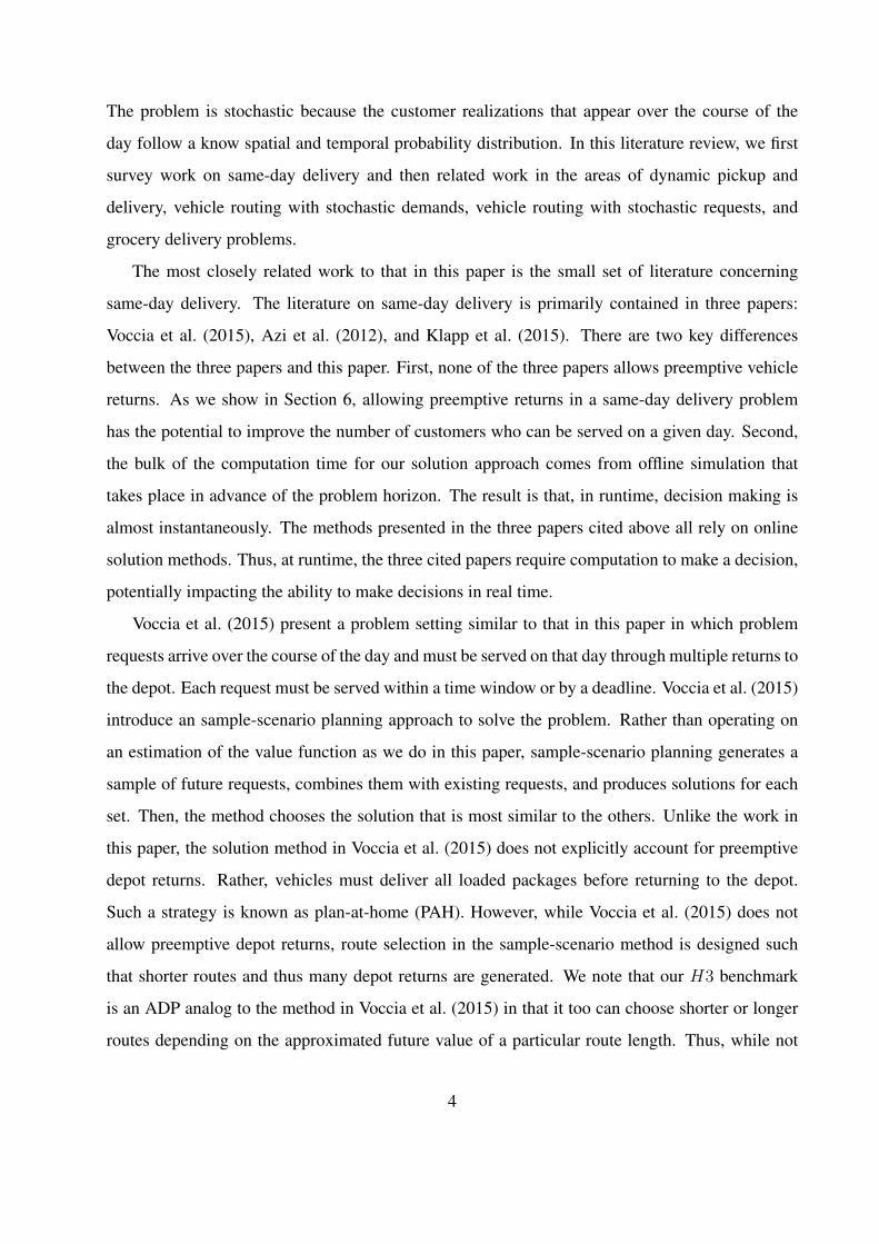
The problem is stochastic because the customer realizations that appear over the course of the

day follow a know spatial and temporal probability distribution. In this literature review, we first

survey work on same-day delivery and then related work in the areas of dynamic pickup and

delivery, vehicle routing with stochastic demands, vehicle routing with stochastic requests, and

grocery delivery problems.

The most closely related work to that in this paper is the small set of literature concerning

same-day delivery. The literature on same-day delivery is primarily contained in three papers:

Voccia et al. (2015), Azi et al. (2012), and Klapp et al. (2015). There are two key differences

between the three papers and this paper. First, none of the three papers allows preemptive vehicle

returns. As we show in Section 6, allowing preemptive returns in a same-day delivery problem

has the potential to improve the number of customers who can be served on a given day. Second,

the bulk of the computation time for our solution approach comes from offline simulation that

takes place in advance of the problem horizon. The result is that, in runtime, decision making is

almost instantaneously. The methods presented in the three papers cited above all rely on online

solution methods. Thus, at runtime, the three cited papers require computation to make a decision,

potentially impacting the ability to make decisions in real time.

Voccia et al. (2015) present a problem setting similar to that in this paper in which problem

requests arrive over the course of the day and must be served on that day through multiple returns to

the depot. Each request must be served within a time window or by a deadline. Voccia et al. (2015)

introduce an sample-scenario planning approach to solve the problem. Rather than operating on

an estimation of the value function as we do in this paper, sample-scenario planning generates a

sample of future requests, combines them with existing requests, and produces solutions for each

set. Then, the method chooses the solution that is most similar to the others. Unlike the work in

this paper, the solution method in Voccia et al. (2015) does not explicitly account for preemptive

depot returns. Rather, vehicles must deliver all loaded packages before returning to the depot.

Such a strategy is known as plan-at-home (PAH). However, while Voccia et al. (2015) does not

allow preemptive depot returns, route selection in the sample-scenario method is designed such

that shorter routes and thus many depot returns are generated. We note that our H3 benchmark

is an ADP analog to the method in Voccia et al. (2015) in that it too can choose shorter or longer

routes depending on the approximated future value of a particular route length. Thus, while not

4

implementing it directly, we do use a benchmark that is similar to the approach presented in Voccia

et al. (2015) with the advantage that the calculation is conducted offline.

Also related to this paper is the work of Azi et al. (2012). Similar to this paper and Voccia et al.

(2015), Azi et al. (2012) study a problem in which requests are received throughout the day and are

served through multiple trips to a depot. Similar to Voccia et al. (2015), Azi et al. (2012) develop

a sample-scenario planning approach, and like Voccia et al. (2015), do not explicitly consider

preemptive returns to the depot. Instead, Azi et al. (2012) constrain the length of the tours on the

vehicles leaving the depot. In this way, Azi et al. (2012) implicitly recognize the value of depot

returns, but in contrast to this paper and Voccia et al. (2015), the length of tour limitations proposed

in Azi et al. (2012) are fixed throughout the horizon and do not adapt to changing state information.

Klapp et al. (2015) also explore the same-day delivery problem, but assume that all customers

are on a line. Thus, the routing and subset selection problem are integrated in a single decision,

importantly eliminating the expensive step of evaluating the cost of a chosen subset of customers,

a step that is necessary when considering a general network as we do in this problem. Further,

the formulation does not allow for preemptive depot returns. Given their problem setting, Klapp

et al. (2015) demonstrate how to efficiently find optimal a priori routes and then introduce an

approximate dynamic programming approach known as rollout (see Goodson et al. (2016b) for an

overview of rollout algorithms) to leverage the a priori routes in a dynamic setting.

The SDPD can also be seen as a special case of a dynamic pickup and delivery problem.

In stochastic and dynamic many-to-many pickup and delivery problems (DPDPs), usually both

origin and destination of a request (order) are stochastic. Thus, the main difference between the

SDPD and DPDPs is that, in the SDPD, the pickup location is known beforehand. An overview

on dynamic pickup and delivery problems is given by Berbeglia et al. (2010). Work considering

stochastic requests is conducted, e.g., by Saez et al. (2008), Pureza and Laporte (2008), Mes et al.

(2010). From a methodological perspective, the singular pickup location in the SDPD allows us

to propose a unique state-space aggregation scheme that allows for improved estimation of future

costs. Further, we proposed a solution method that relies on offline computation.

The concept of preemptive depot returns is mainly found in the literature on vehicle routing

with stochastic demands (VRPSD). For these problems, the customers are known but the amount

of demand at each customer is unknown prior to arrival. Thus, the vehicles may need to return to

5

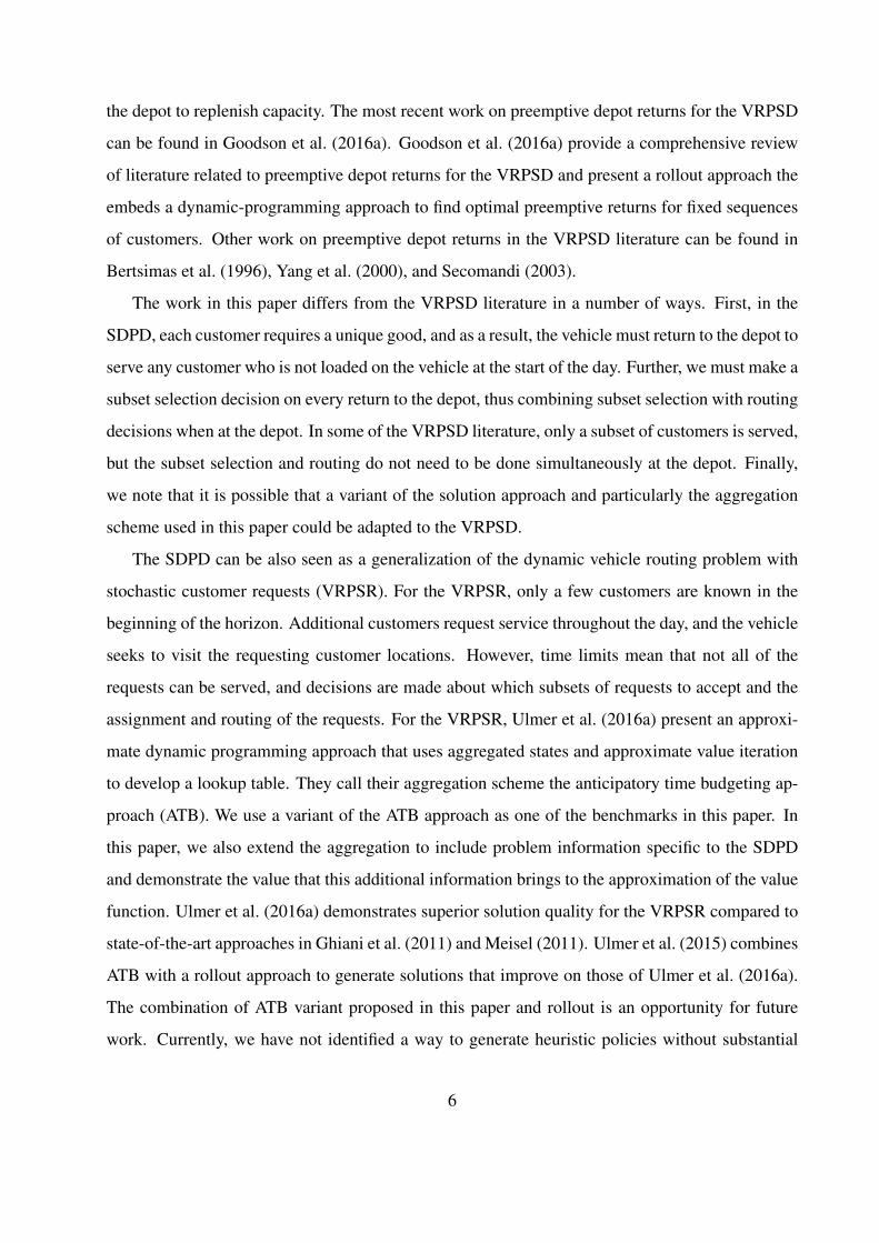
the depot to replenish capacity. The most recent work on preemptive depot returns for the VRPSD

can be found in Goodson et al. (2016a). Goodson et al. (2016a) provide a comprehensive review

of literature related to preemptive depot returns for the VRPSD and present a rollout approach the

embeds a dynamic-programming approach to find optimal preemptive returns for fixed sequences

of customers. Other work on preemptive depot returns in the VRPSD literature can be found in

Bertsimas et al. (1996), Yang et al. (2000), and Secomandi (2003).

The work in this paper differs from the VRPSD literature in a number of ways. First, in the

SDPD, each customer requires a unique good, and as a result, the vehicle must return to the depot to

serve any customer who is not loaded on the vehicle at the start of the day. Further, we must make a

subset selection decision on every return to the depot, thus combining subset selection with routing

decisions when at the depot. In some of the VRPSD literature, only a subset of customers is served,

but the subset selection and routing do not need to be done simultaneously at the depot. Finally,

we note that it is possible that a variant of the solution approach and particularly the aggregation

scheme used in this paper could be adapted to the VRPSD.

The SDPD can be also seen as a generalization of the dynamic vehicle routing problem with

stochastic customer requests (VRPSR). For the VRPSR, only a few customers are known in the

beginning of the horizon. Additional customers request service throughout the day, and the vehicle

seeks to visit the requesting customer locations. However, time limits mean that not all of the

requests can be served, and decisions are made about which subsets of requests to accept and the

assignment and routing of the requests. For the VRPSR, Ulmer et al. (2016a) present an approxi-

mate dynamic programming approach that uses aggregated states and approximate value iteration

to develop a lookup table. They call their aggregation scheme the anticipatory time budgeting ap-

proach (ATB). We use a variant of the ATB approach as one of the benchmarks in this paper. In

this paper, we also extend the aggregation to include problem information specific to the SDPD

and demonstrate the value that this additional information brings to the approximation of the value

function. Ulmer et al. (2016a) demonstrates superior solution quality for the VRPSR compared to

state-of-the-art approaches in Ghiani et al. (2011) and Meisel (2011). Ulmer et al. (2015) combines

ATB with a rollout approach to generate solutions that improve on those of Ulmer et al. (2016a).

The combination of ATB variant proposed in this paper and rollout is an opportunity for future

work. Currently, we have not identified a way to generate heuristic policies without substantial

6

computation, thus limiting the ability to develop a rollout approach that can be executed in real

time.

Older VRPSR literature relied on waiting strategies, strategies that have the vehicle wait in

particular locations in anticipation of future requests. Mitrovic-Minic and Laporte (2004) provide

a nice overview of the strategies. Of the strategies, only the wait-at-start heuristic (WAS) presented

by Mitrovic-Minic and Laporte (2004) can be adapted to the problem in this paper. For WAS, the

vehicles idles at the depot as long as possible. It is possible to adapt WAS because all assignments

take place when the vehicle is located at the depot. For the SDPD, the application of WAS does

not require any depot returns after the vehicle has left the depot. However, preliminary tests reveal

WAS to perform poorly for the SDPD.

Also related to same-day delivery is the grocery-delivery problem. While the deliveries for

grocery delivery usually take place the day after orders are made, at the time an order is placed, the

decision maker must determine whether or not the order can be feasibly served on the next day’s

routes given the existing requests. In that case, the evaluation of each request is related to the need

in this problem to evaluate the routing cost of a subset of customers. Recent work can be found in

(Ehmke et al. 2015) and (Ehmke and Campbell 2014).

3 Problem Description and Model

In this section, we present the SDPD and model it as a Markov Decision Process (MDP).

3.1 Problem Description

We assume that a single vehicle delivers customer orders in a service areaA. The vehicle starts the

tour at a depot D, travels with constant speed ν and returns before the time limit tmax. The travel

time between two customers C1, C2 ∈ A is determined by a specific d(C1, C2) ∈ N+. The service

time at a customer is ζc. In the beginning, a set of initial orders (IOs) C0 ∈ A is known and must

be served. We assume that these IOs are loaded on the vehicle at the beginning of the day. During

the day, stochastic orders (SOs) C+ occur in A. When the vehicle is located at a customer or at

the depot, the dispatcher determines which customer to visit next or whether to return to the depot.

When at the depot, the vehicle can be loaded with packages destined for realized and assigned

7

Table 1: MDP: Customer Set Notation

Notation Description

C0 Set of initial orders

C+ Set of stochastic orders

Cl(k) Set of loaded orders in Sk

Cι(k) Set of not loaded but preliminarily assigned orders in Sk

Cε(k) Set of not loaded and preliminarily excluded orders in Sk

Cr(k) ⊂ Cε(k) Set of new requests in Sk

SOs. The loading time at a the depot ζd is independent of the number of loaded orders. We assume

that the IOs are loaded before the start of the horizon. In determining which SOs should be served,

the dispatcher ensures the existence of a feasible tour serving all assigned IOs, previously loaded

SOs, and newly loaded SOs. We assume that once loaded on the vehicle, the packages destined for

SOs must be delivered. The objective is to maximize the expected number of SOs served over the

horizon of the problem.

3.2 Markov Decision Process Model

In this section, we model the SDPD as a Markov Decision Process (MDP). The MDP for the

SDPD can be formulated such that assignment decisions are made only when the vehicle is located

at the depot. That is, when the orders are loaded. For algorithmic purposes, however, we consider

preliminary assignments of customers at every decision point. These preliminary assignments

are not binding and can be changed at future decisions, provided that the assigned customers

have not yet been loaded on the vehicle. To facilitate these preliminary assignments, we present

an alternative MDP-formulation that integrates a planned tour θk into the state variable Sk, the

decision variable x, and in the reward function R = (Sk, x). Because the planned tour is used only

for the purposes of a heuristic solution method, it does not alter the validity of the model and could

be omitted.

A decision point or decision epoch k occurs when the vehicle visits a customer or the depot.

8

The decision state Sk ∈ S is defined as follows. At a minimum, the state must contain all of the

data necessary for determining feasible decisions, the cost of those decisions as well as defining

the transitions to future states. For the SDPD, we can think of the state in terms resources and

information. The resources associated with the SDPD are the available time t(k) and the location

of the vehicle Pk. The information in the SDPD is the information about service requests and the

statuses of those requests. For this purpose, we have three sets per state, summarized in Table 1.

We let Cl(k) ⊂ C0 ∪ C+ be the set of customers whose packages have been loaded on the vehicle

for delivery. We call these loaded customers. We denote the set of assigned, but not loaded SOs

as Cι(k) ⊂ C+ and the set of excluded SOs, Cε(k). The set Cε(k) denotes the currently excluded

SOs containing Cr(k) ⊂ Cε(k), the SOs realized between t(k − 1) and t(k) for k > 0. As noted

previously, we also include in the state the planned feasible tour θk = (Pk, . . . ,D). This planned

tour θk = (C1, . . . , Cn,D, Cn+1, . . . , Cn+m,D) defines the planned sequence of customer and

depot returns and may contain preliminarily assigned SOs. These preliminary SOs are SOs that

are part of the tour for planning purposes but are not yet loaded to the vehicle. These preliminary

SOs may in fact not be served by the vehicle if later decision change their assignment status. Thus,

the state at decision point k is given by the tuple Sk = (t(k), θk,Pk, Cl(k), Cι(k), Cε(k)).

Decisions x ∈ X(Sk) are made about the subsets C(ι,x)(k) ⊂ Cε(k) ∪ Cι(k) to preliminary

assign, the resulting subset C(ε,x)(k) to preliminary exclude, and the according update of θk to

θxk . The update of the planned tour determines the next location to visit. This location Cnext ∈

D ∪ Cl(k) ∪ Pk can be chosen from the set of loaded customers, the depot, or the current

location, a choice which implies that the vehicle idles at the current location for a length of time t.

If the vehicle is located at the depot, Pk = D, the selection of assigned SOs C(ι,x)(k) at epoch k are

loaded to the vehicle. Decision x is feasible if θxk starts inPk, serves all customers Cl,x(k)∪C(ι,x)(k),

and returns to the depot within the time limit. Formerly, feasibility is given by:

d(θxk) ≤ tmax − t(k).

Each decision results in an immediate reward. This reward is equal to the number of newly

assigned SOs minus the number of excluded formally included SOs. Formally, the rewardR(Sk, x)

is defined as

9

R(Sk, x) = |C(l,x)(k)|+ |C(ι,x)(k)| − |Cl(k)| − |Cι(k)|.

The execution of x results in a post-decision state Sxk ∈ Sx. The post decision-state represents

the deterministic transition from Sk that results from the execution of x. Notably, the post-decision

state captures the updated route plan and the updated sets of loaded, assigned, and excluded cus-

tomers resulting from x: C(l,x)(k), C(ι,x)(k), C(ε,x)(k). If x calls for the loading of orders, the accord-

ing sets of loaded and not loaded customers are modified as follows. The customers corresponding

to the loaded goods are transferred from Cι(k) to C(l,x)(k) and C(ι,x)(k) = ∅. The transition also

updates the vehicle location to the next visit location resulting from x. Formally, given Sk and x,

the post-decision state is

Sxk = (t(k), θxk , Cnext, C(l,x)(k), C(ι,x)(k), C(ε,x)(k)).

At the next decision epoch, the point of time at which the vehicle arrives to the next location

and finished service at that location. The time of this decision point is a function of the location to

which the vehicle is traveling and is deterministic. The next decision points occurs at t(k + 1) =

t(k) + d(Pk, Pk+1) + ζ with ζ ∈ ζc, ζd, 0 dependent on the next location Pk+1. Time ζ = 0 is

the special case, when k+ 1 = K. That is, the vehicle eventually returns to the depot at the end of

the horizon.

With the new decision point, there occurs a stochastic transition from the post-decision state

to the next pre-decision state. This transition is defined by the realization ωk+1 ∈ Ωk+1. This

realization identifies the set of customer orders that were realized between t(k) and t(k + 1).

Specifically, the realization ωk+1 provides a set of customers Cr(k + 1) = C1, . . . , Ch. The next

state Sk+1 contains the time t(k + 1), the remaining loaded and unloaded customers dependent on

C(l,x)(k), C(ι,x)(k), the vehicle’s location Pk+1 = Pxk , and the planned tour θk+1. If no customer is

visited in t(k + 1), Cl(k + 1) = C(l,x)(k) and θk+1 = θxk remain. Otherwise, the visited customer

Ck+1 is removed from the according set as θk+1 = θxk\Ck+1.

The initial state S0 is defined by t(0) = 0, P0 = D, the initial orders C0, and the initial tour

θ0 = (D,D). Termination state SK is defined by t(K) = tmax, PK = D, Cl(K) = ∅, and θK = (D).

The objective for the SDPD is to determine an optimal decision policy π∗ ∈ Π leading to the

highest expected sum of rewards. Formally, the objective is

10

P P PPosition

Customer(loaded)

Customer(notloaded)

Customer(excluded)

Depot

t=120 t=120

x

Figure 1: Exemplary State, Decision, and Post-Decision State

π∗ = arg maxπ∈Π

E

[K∑k=0

R(Sk, Xπk (Sk))|S0

]. (1)

Decision rule Xπk (Sk) determines the decision x selected by policy π in state Sk.

3.3 Example

In this section, we present an example of the components of the MDP for the SDPD. The example

is given in Figure 1. The example depicts the exemplary state at time t(k) = 120, the vehicle

having just served a customer. The planned tour θk is depicted by the dashed lines. Tour θk plans

to visit the loaded customer on the left side of the area, return to the depot, and visit the unloaded

but assigned customer and the loaded customer in the bottom of the area. Currently, two SOs

are excluded, located in the right of the service area. They may be new SOs or orders formerly

excluded.

The selection of x leads to a post-decision state Sxk . In Figure 1, this post-decision state is

represented on the right-hand side of the block arrow. Decision x excludes the customer on the

bottom left that is not currently loaded and includes the SOs located on the right side of the service

area. The next location to visit is the customer on the left side. The dashed lines represent the

feasible tour θxk . This planned tour may change as the vehicle returns to the depot before serving

the currently assigned but not yet loaded customers. Since two orders are assigned and one is

11

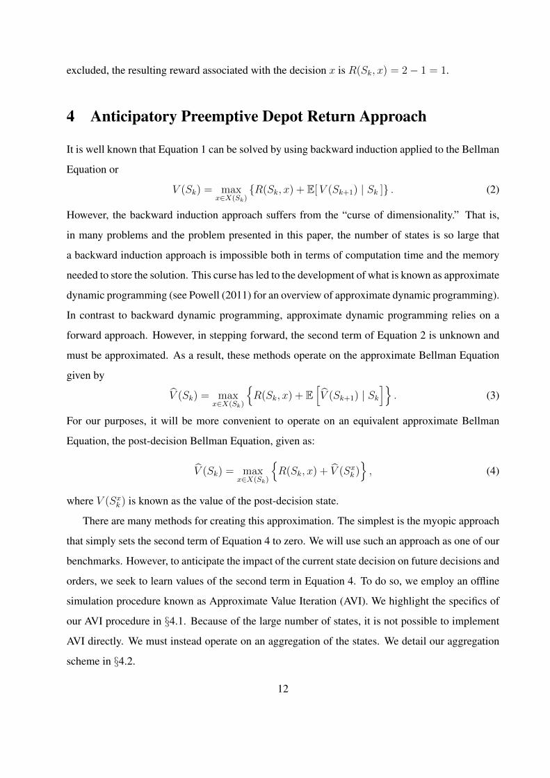
excluded, the resulting reward associated with the decision x is R(Sk, x) = 2− 1 = 1.

4 Anticipatory Preemptive Depot Return Approach

It is well known that Equation 1 can be solved by using backward induction applied to the Bellman

Equation or

V (Sk) = maxx∈X(Sk)

R(Sk, x) + E[V (Sk+1) | Sk ] . (2)

However, the backward induction approach suffers from the “curse of dimensionality.” That is,

in many problems and the problem presented in this paper, the number of states is so large that

a backward induction approach is impossible both in terms of computation time and the memory

needed to store the solution. This curse has led to the development of what is known as approximate

dynamic programming (see Powell (2011) for an overview of approximate dynamic programming).

In contrast to backward dynamic programming, approximate dynamic programming relies on a

forward approach. However, in stepping forward, the second term of Equation 2 is unknown and

must be approximated. As a result, these methods operate on the approximate Bellman Equation

given by

V (Sk) = maxx∈X(Sk)

R(Sk, x) + E

[V (Sk+1) | Sk

]. (3)

For our purposes, it will be more convenient to operate on an equivalent approximate Bellman

Equation, the post-decision Bellman Equation, given as:

V (Sk) = maxx∈X(Sk)

R(Sk, x) + V (Sxk )

, (4)

where V (Sxk ) is known as the value of the post-decision state.

There are many methods for creating this approximation. The simplest is the myopic approach

that simply sets the second term of Equation 4 to zero. We will use such an approach as one of our

benchmarks. However, to anticipate the impact of the current state decision on future decisions and

orders, we seek to learn values of the second term in Equation 4. To do so, we employ an offline

simulation procedure known as Approximate Value Iteration (AVI). We highlight the specifics of

our AVI procedure in §4.1. Because of the large number of states, it is not possible to implement

AVI directly. We must instead operate on an aggregation of the states. We detail our aggregation

scheme in §4.2.

12

Unfortunately, in addition to the proliferation of states, the problem discussed in this paper also

suffers from another curse of dimensionality, the size of the decision space. Notably, not only must

we selection a subset at each decision epoch, but we must also route that selected subset. In this

paper, we heuristically reduce the possible decision space by using a simple routing heuristic that

it incorporates depot returns. The details of our procedure can be found in §4.3. Combining the

three elements of the solution approach, we call our solution approach the anticipatory preemptive

depot return approach (APDR).

4.1 Approximate Value Iteration

In this section, we define our method for determining the approximate value of the second term in

Equation 4. In this section, we present the method generally and as if we are determining an ap-

proximate value for each post-decision state. However, in execution, we operate on an aggregated

set of states. We define this aggregation in the following section.

Our AVI method is derived from (Powell 2011, pp. 391ff) and uses offline simulation to deter-

mine approximated values. The approximated values are stored in a lookup table and can then be

used to solve Equation 4 in real time. Thus, the computational burden of the approach is mainly

done prior to when decision making is required and greatly reduces the computational computa-

tional burden at runtime.

The procedure is described in Algorithm 1. AVI starts with initial values V0(Sxk ) for every post-

decision state Sxk . Then, AVI iterates through a set of sample path realizations Ω = ω1, . . . , ωN.

Then, at each iteration i and each step in a given sample path realization ωi, the algorithm solves

the approximate Bellman equation (line 12) using the current approximation of the post-decisions

states Vi−1. The value of the selected decision, given in line 14, is used in line 20 to update the ap-

proximated post-decision state values. The algorithm returns values VN that we use to approximate

the second term of Equation 4 at runtime.

4.2 State Space Aggregation

Because of the large numbers of post-decision states required, we cannot actually find values for

each post-decision state and instead develop the approximation on aggregated post-decision states.

13

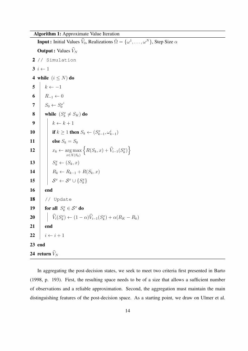
Algorithm 1: Approximate Value Iteration

Input : Initial Values V0, Realizations Ω = ω1, . . . , ωN, Step Size α

Output : Values VN

22 // Simulation

3 i← 1

4 while (i ≤ N) do

5 k ← −1

6 R−1 ← 0

7 S0 ← Sωi

0

8 while (Sxk 6= SK) do

9 k ← k + 1

10 if k ≥ 1 then Sk ← (Sxk−1, ωik−1)

11 else Sk = S0

12 xk ← arg maxx∈X(Sk)

R(Sk, x) + Vi−1(Sxk )

13 Sxk ← (Sk, x)

14 Rk ← Rk−1 +R(Sk, x)

15 Sx ← Sx ∪ Sxk

16 end

1818 // Update

19 for all Sxk ∈ Sx do

20 Vi(Sxk )← (1− α)Vi−1(Sxk ) + α(RK −Rk)

21 end

22 i← i+ 1

23 end

24 return VN

In aggregating the post-decision states, we seek to meet two criteria first presented in Barto

(1998, p. 193). First, the resulting space needs to be of a size that allows a sufficient number

of observations and a reliable approximation. Second, the aggregation must maintain the main

distinguishing features of the post-decision space. As a starting point, we draw on Ulmer et al.

14

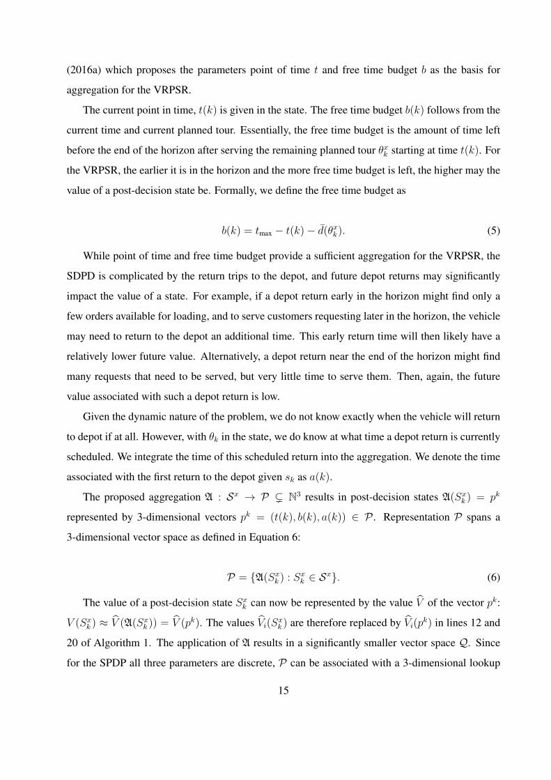
(2016a) which proposes the parameters point of time t and free time budget b as the basis for

aggregation for the VRPSR.

The current point in time, t(k) is given in the state. The free time budget b(k) follows from the

current time and current planned tour. Essentially, the free time budget is the amount of time left

before the end of the horizon after serving the remaining planned tour θxk starting at time t(k). For

the VRPSR, the earlier it is in the horizon and the more free time budget is left, the higher may the

value of a post-decision state be. Formally, we define the free time budget as

b(k) = tmax − t(k)− d(θxk). (5)

While point of time and free time budget provide a sufficient aggregation for the VRPSR, the

SDPD is complicated by the return trips to the depot, and future depot returns may significantly

impact the value of a state. For example, if a depot return early in the horizon might find only a

few orders available for loading, and to serve customers requesting later in the horizon, the vehicle

may need to return to the depot an additional time. This early return time will then likely have a

relatively lower future value. Alternatively, a depot return near the end of the horizon might find

many requests that need to be served, but very little time to serve them. Then, again, the future

value associated with such a depot return is low.

Given the dynamic nature of the problem, we do not know exactly when the vehicle will return

to depot if at all. However, with θk in the state, we do know at what time a depot return is currently

scheduled. We integrate the time of this scheduled return into the aggregation. We denote the time

associated with the first return to the depot given sk as a(k).

The proposed aggregation A : Sx → P ( N3 results in post-decision states A(Sxk ) = pk

represented by 3-dimensional vectors pk = (t(k), b(k), a(k)) ∈ P . Representation P spans a

3-dimensional vector space as defined in Equation 6:

P = A(Sxk ) : Sxk ∈ Sx. (6)

The value of a post-decision state Sxk can now be represented by the value V of the vector pk:

V (Sxk ) ≈ V (A(Sxk )) = V (pk). The values Vi(Sxk ) are therefore replaced by Vi(pk) in lines 12 and

20 of Algorithm 1. The application of A results in a significantly smaller vector space Q. Since

for the SPDP all three parameters are discrete, P can be associated with a 3-dimensional lookup

15

table (LT) with dimensions t, b, a ∈ 0, . . . , tmax. Based on the aggregated post-decision states in

the LT, we are now able to store the values for AVI.

4.3 Subset Selection and Preemptive Depot Return Routing

The final component of our solution approach overcomes the challenge of the large decision space

present in this problem. The decision space’s dimensionality is vast due to two reasons. First, as

long as a request is not loaded onto the vehicle, the MDP model allows for reconsideration of SO-

assignments. In combination with new SOs, this leads to a significant subset selection subproblem.

Second, the set of potential routing plans is vast, especially when considering potential depot

returns.

Given this curse of dimensionality in the decision space, in the APDR, we use a heuristic to

limit the number of subsets and routing schemes that must be considered when solving line 12

of Algorithm 1 and in runtime when solving Equation 4. These heuristics can be thought of as a

means to restricting the decision space at each decision epoch.

To alleviate the subset selection complexity, at every decision point, APDR and the benchmark

policies presented in §4.4 maintain the already assigned SOs and determine only the subset of new

SOs to assign. An SO that unassigned SO at a particular decision point is permanently excluded

if not assigned at that decision point. We do not reconsider assignments and exclusions due to the

combinatorial complexity of considering all possible subsets.

For each state on each sample path of each iteration of Algorithm 1, a decision is selected in

line 12. This decision involves the selection and routing of a subset of customers. As discussed

previously, the size of the decision space is such that it is impossible to solve Equation 4 optimally.

Instead, for each subset of new customer requests, we heuristically generate the new planned tour

θxk , for a state Sk, a current tour θk, and a set of SOs Cr. We call the approach the preemptive depot

return routing approach (PDR).

To heuristically generate tours for a set of SOs, PDR draws on a modification of cheapest in-

sertion (CI), which is first introduced by Rosenkrantz et al. (1974). We derive our implementation

from that proposed in Azi et al. (2012). CI has the advantage of being efficient at every decision

point. Further, the resulting routes are such that they are comprehensible to the driver. Because CI

maintains the sequence of customers, the dispatcher might even be able to communicate approxi-

16

1. 2. 3. 4.

Figure 2: Routing and Insertion for PDR

mate delivery times (Ulmer and Thomas 2016). A downside of PDR is that it does not necessarily

return optimal routes and thus may reduce the set of feasible orders.

The procedure of PDR is described in Algorithm 2 found in the Appendix. Let D denote the

depot, Pk the vehicle’s position, Cl the loaded IOs. Further, we let Cn represent the assigned

unloaded SOs. The current planned tour can then be described as

θk = (Pk, Cl, . . . , Cl,D, Cn, Cl, Cn, . . . , Cl,D).

Let θjk refer to the j th component of θk, e.g., θ1k = Pk. Further, let Cr = C1

r , . . . , Chr be the

subset of new SOs to assign. PDR first removes the depot from θk leading to an infeasible tour θ.

In this infeasible tour, the customers Cr are subsequently inserted via CI at the cheapest position.

Procedure Insert(θ, θ∗, C∗) inserts the new order C∗ after θ∗ in tour θ. When all new customers

are inserted, the depot is inserted between the current position and the first not loaded customer

(Cn or Cr) via CI resulting in a tour θxk . If θxk does not violate the time limit, the tour is feasible.

We assume an initial tour θ0 = (D,D) without customers, starting and ending at the depot. Due

to the stochasticity of the problem, the integration of the IOs at k = 0 may lead to an initial tour

duration higher then the time limit. In these cases, the vehicle serves all IOs and none of the SOs.

For k > 0, there always exists a feasible decision x assigning no new SOs to the tour. In these

cases, θxk is equal to θk.

Figure 2 shows an example for PDR. The first step shows state Sk, θk, and the candidate set of

new SOs Cr. The state contains three loaded, one assigned but not loaded, and one new customer.

The current depot return is planned after serving the customer located at the top left of the service

area. In the second step, PDR removes the depot within the sequence θk. This resulting tour

is infeasible because a depot return is required to pickup customer orders at the depot. In the

17

third step, PDR then inserts the candidate subset of new customers via CI. The resulting tour is

again infeasible. Feasibility is restored by the addition of a depot return before the first not loaded

customer in the tour. The fourth step shows the depot return being inserted between Pk and the

first not loaded customer Cn.

4.4 Benchmark Heuristics

In this section, we present the benchmark heuristics that we use to test the quality of the proposed

approach. As with our proposed approach, each benchmark includes a strategy for estimating

the future value of a decision and a strategy for heuristically routing a subset of requests. For

anticipation, we consider both ATB aggregation proposed by Ulmer et al. (2016b) for the VRPSR

and a myopic assignment strategy. For routing, we consider both the preemptive method proposed

in the previous section and the well-established plan-at-home heuristic (PAH). The combination

of these anticipation and routing strategies results in four benchmarks. We also consider a fifth

benchmark derived from combining the proposed three-parameter aggregation scheme described

in §4.2 with the PAH routing scheme described subsequently.

Anticipation: Myopic and ATB

We compare our proposed anticipation approach to both ATB and myopic anticipation. As de-

scribed previously, ATB is similar to the approach proposed in this paper, but the aggregation does

not include information about depot returns. Thus, ATB aggregates over only the point of time and

the free time budget. For this paper, the lookup table for ATB is created using a AVI-procedure

analogous to that described in Algorithm 1.

For an additional point of comparison, we also consider using a myopic policy for anticipation.

The myopic approach sets the second term of Equation 4 to zero. The myopic assignment strategy

selects decision x leading to the assignment of the largest feasible subset in every decision point k.

If several decisions with the same subset cardinality exist, the strategy selects the decision of these

leading to the highest free time budget.

18

Depot Returns: Plan at Home

This paper introduces a preemptive return strategy. As a benchmark, we consider the PAH. In the

benchmark, we replace the subset selection and routing discussed in §4.3 with PAH. Particularly,

PAH is an approach that does not account for the possibility of preemptive depot returns. Thus, at

time of the return to the depot, the vehicle is empty. Upon return, a set of new requests is selected

for service, and the vehicle begins a new route.

Specifically, the PAH approach is a modification of Algorithm 2. The modification removes

lines 2 through 6 and lines 18 through 25. In addition, line 10 is modified such that j = k, . . . , |θ|−

1, where k is the position in θ of the depot. We note that the modification of line 10 means that

PAH does not serve IOs and SOs on the same tours. Like the approach discussed in §4.3, PAH

is a means of restricting the decision space. At each decision epoch, the PAH approach seeks to

accept some newly occurring requests for inclusion on the tour that will take place once the vehicle

returns to the depot. The routing of these accepted requests follows the just described version of

Algorithm 2. In the case of a myopic assignment strategy, the selection of requests amounts to

choosing the maximal feasible subset of requests. In the case of the three-parameter aggregation

strategy and ATB, the subset selection follows the scheme discussed in §4.3 and the routing is

replaced by the modification of Algorithm 2 described in the previous paragraph.

As noted in §2, Azi et al. (2012), Voccia et al. (2015), and Klapp et al. (2015) implement PAH

strategies. Our three-parameter and ATB anticipation schemes mimic the schemes in Azi et al.

(2012), Voccia et al. (2015), and Klapp et al. (2015) that, while not making preemptive depot

returns, control the length of the route to induce a depot return in the PAH scheme.

Policy Notation

The combination of routing and assignment strategies results in six different policies Pg,Hg, g =

1, 2, 3. Parameter g indicates the assignment strategy, P and H the routing. The value g = 1

indicates myopic assignments, g = 2 the ATB-assignment based on the 2-dimensional aggregation,

and g = 3 the assignments based on 3-dimensional aggregation presented in §4.2. Indicator P

represents preemptive PDR-routing and H PAH-routing.

19

5 Experimental Design

In this section, we describe the test instances and implementation that we use to demonstrate the

value of preemptive depot returns and of our proposed solution approach. We first present the

scheme for generating instances and then the details of the implementation of our APDR approach

as well as the proposed benchmarks.

5.1 Instance Generation

For all instances, we assume a closed, rectangular service area A assumed to be 20km × 20km, a

time horizon of 480 minutes discretized into 1 minute increments, and a vehicle speed ν of 20km/h.

Assuming a minimum travel time of 1 minute, the travel time between any two points (ax1 , ay1) and

(ax2 , ay2) in A is given by

d(C1, C2) = max

(⌈((ax1 − ax2)2 + (ay1 − a

y2)2)1/2

60−1ν

⌉, 1

). (7)

For all instances, we also assume the service time at a customer is ζc = 2 minutes and the loading

time at the depot is ζd = 5 minutes.

Each instance is defined by a set of parameters: expected number of customers c, the degree

of dynamism dod, depot locations D, and customer distribution F . The expected number of cus-

tomers is the sum of the IOs and SOs. We test instances with c = 30, 40, 50, 60, 80, 100 expected

customers. The degree of dynamism, first discussed in Larsen et al. (2002), is the percentage of the

expected number of customers that are dynamic. That is, the degree of dynamism is the percent

of customers who are SOs. We test instances with dod = 0.25, 0.5, 0.75. We denote the expected

number of IOs as c0 = c · (1− dod).

To analyze the interdependency of depot location and customer distribution, we define three

different depot locations and customer distributions, respectively. We set the depot locations at

D1 = (10, 10), D2 = (0, 20), and D3 = (0, 0). The latter two depot locations represent the

situation in which the vehicle is part of a fleet, but operates independently in a predefined service

area. For customer locations, we consider uniform and clustered customer distributions. We refer

to uniformly distributed customer locations asU . We define two clustered distributions of customer

locations. The first is a two cluster distribution, called 2C, with two clusters centered at µ1 = (5, 5)

20

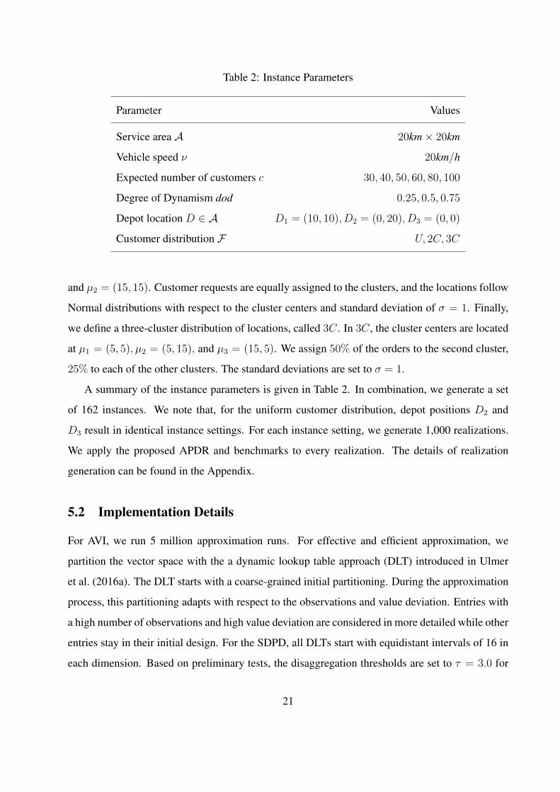
Table 2: Instance Parameters

Parameter Values

Service area A 20km× 20km

Vehicle speed ν 20km/h

Expected number of customers c 30, 40, 50, 60, 80, 100

Degree of Dynamism dod 0.25, 0.5, 0.75

Depot location D ∈ A D1 = (10, 10), D2 = (0, 20), D3 = (0, 0)

Customer distribution F U, 2C, 3C

and µ2 = (15, 15). Customer requests are equally assigned to the clusters, and the locations follow

Normal distributions with respect to the cluster centers and standard deviation of σ = 1. Finally,

we define a three-cluster distribution of locations, called 3C. In 3C, the cluster centers are located

at µ1 = (5, 5), µ2 = (5, 15), and µ3 = (15, 5). We assign 50% of the orders to the second cluster,

25% to each of the other clusters. The standard deviations are set to σ = 1.

A summary of the instance parameters is given in Table 2. In combination, we generate a set

of 162 instances. We note that, for the uniform customer distribution, depot positions D2 and

D3 result in identical instance settings. For each instance setting, we generate 1,000 realizations.

We apply the proposed APDR and benchmarks to every realization. The details of realization

generation can be found in the Appendix.

5.2 Implementation Details

For AVI, we run 5 million approximation runs. For effective and efficient approximation, we

partition the vector space with the a dynamic lookup table approach (DLT) introduced in Ulmer

et al. (2016a). The DLT starts with a coarse-grained initial partitioning. During the approximation

process, this partitioning adapts with respect to the observations and value deviation. Entries with

a high number of observations and high value deviation are considered in more detailed while other

entries stay in their initial design. For the SDPD, all DLTs start with equidistant intervals of 16 in

each dimension. Based on preliminary tests, the disaggregation thresholds are set to τ = 3.0 for

21

both APDR and H3 and τ = 1.5 for both P2 and H2. A disaggregation divides each interval of

the entry in two equidistant halves. The number of observations is distributed equally to the new

entries. The standard deviation of the new entries is set to the standard deviation of the original

entry. The disaggregation of an entry stops when the entry reaches an interval length of 1 minute.

The update parameter α is set to the inverse of the number of observations. Ulmer et al. (2016a)

demonstrates the quality of this step-size rule for AVI coupled with DLT.

6 Computational Evaluation

In this section, we present the results of our computational experiments. We compare the proposed

APDR approach to the five previously described benchmarks. Our results demonstrate the quality

of the proposed approach and also the value of preemptive depot returns. In our presentation, we

characterize the instance parameters that both favor preemptive depot returns and those that do not.

6.1 Overall Solution Quality

In this section, we analyze the solution quality of the six different policies. Detailed results for ev-

ery instance are available in Table A1 in the Appendix. To analyze the improvement, we measure

the five benchmark policies versus the APDR. We first look at the overall quality of each solution

to the others by comparing the average over all instance settings of the percentage differences in

the average number of SOs served per instance setting. To do so, for each benchmark i and for

the APDR, we compute the average number of SOs served over all realizations for each instance

setting. For each benchmark i and instance setting j, we compute this value Qij for each bench-

mark i and QAPDR,j for the APDR approach. Then, for every benchmark i and instance setting j,

we compute the percentage difference between a benchmark i and the APDR as

QAPDR,j −QijQAPDR,j

× 100%. (8)

We then average over these percentage differences to get the average percentage difference between

APDR and each benchmark i.

Figure 3 presents the average percentage difference in solution quality of the approaches. On

the x-axis, each benchmark policy i is depicted. On the y-axis, the percentage improvement relative

22

7.4%

4.6%

9.7%

18.3%

19.3%

0%

5%

10%

15%

20%

P2

P1

H3

H2

H1

Diff

eren

ce R

elat

ive

to P

3

Figure 3: Percentage Difference of the Average Stochastic Orders Served by APDR and the Bench-

mark Policies

to APDR is shown. Positive values show that APDR is outperforming the benchmark.

The values indicate that the proposed APDR approach is best overall. The improvement of

APDR is at least 4.6% and with a difference of 19.3% when compared to H1. The results also

show that the quality of the APDR approach is due both to the preemptive returns and also to

the inclusion of planned depot return information in the aggregation. With P1 being 4.6% worse

than APDR and P2 being 7.4% worse than APDR, both less than the difference between the

APDR and the plan-at-home approaches, the results also show the relative advantage of preemptive

depot returns. In §6.3, we analyze the reason that preemptive depot returns are beneficial and also

characterize the instance settings in which preemptive returns provide the most value.

We also observe a significant gap between APDR and benchmarks P2 and P1 as well as

between H3 and benchmarks H2 and H1. Notably, the improvement from APDR to P2 is 7.4%,

even higher than compared that of APDR compared to P1. Recall that policy P2 is based on the

2-dimensional aggregation of the state space. This aggregation ignores the planned arrival time

of a return to the depot. Likewise, H3 is 8.6% and 9.6% percentage points better than H2 and

H1, respectively. These significant improvements of the 3-dimensional aggregation over the 2-

23

dimension case indicate the benefit of capturing the planned depot return time in the aggregation.

In §6.2, we investigate how including the planned arrival time in the aggregation impacts the value

of a state and the resulting subset selection.

6.2 The Value of Including Planned Depot Arrival Time in the State Space

Aggregation

In this section, we analyze why the benefit of 3-dimensional aggregation, the inclusion of the

planned depot arrival time in the aggregation. To do this, we use an example to show how the

value of the aggregated states changes with the planned depot arrival times for both the APDR

and H3 approaches. Showing these changes demonstrates the sensitivity of the post-decision state

value to the planned depot return time.

Specifically, we focus on the instance setting in which c = 50, dod = 0.5, the customers are

distributed in two clusters (2C), and the depot is in the center (D1). For this instance setting, the

solution quality of APDR and H3 are nearly similar with 10.0 and 10.1 assignments on average,

respectively. For the purposes of the example, we focus on time t = 180. At t = 180, for H3,

the vehicle has usually not returned to the depot yet. We select a free time budget of b = 100

since preliminary tests have revealed frequent observations for the combination of t = 180 and

b = 100. With the time and time budget fixed, only the planned arrival time to the depot varies in

our example. As a result, only arrival times of 180 ≤ a ≤ 380 = 480− b are possible.

For the just described setting, Figure 4 presents the post-decision state values across planned

arrival time values for both the APDR and H3 at time 180 and time budget 100. The x-axis shows

the planned arrival time a and the y-axis the value for the according vector. That is, y-axis shows

how many assignments are expected for the corresponding post-decision states. The solid line

depicts the value of the APDR approach and the dashed line H3. The occasional plateaus in the

values are the result of the varying interval sizes of the DLT.

Figure 4 shows that the value of the post-decision state is sensitive to the planned arrival time.

For example, the post-decision state value of the APDR at a = 200 is 3.86 while for a = 350,

the value is 4.82, a difference of nearly 25%. Likewise, the post-decision state value of the H3 at

a = 200 is 4.12 while for a = 350, the value is 4.74, a difference of nearly 15%. In contrast, P2

24

Figure 4: Value for APDR and H3, Instance Setting c = 50, dod = 0.5, 2C,D1. Point of Time

t = 180, Free Budget b = 100

and H2 neglect parameter a and evaluate every post-decision state with t = 180, b = 100 with the

values 4.62 or 3.83, respectively. As a result, the performance of these benchmarks is inferior to

APDR and H3, respectively.

The question remains as to why the value of the post-decision state is sensitive to the time of the

planned depot return. To answer this question, we first examine H3. We observe an increase in the

value of the post-decision state until about time a = 260. For 260 ≤ a ≤ 300, the value remains

relatively constant and drops for a > 300. This behavior can be explained by two influencing

factors. First, as more time that passes, more new requests will be accumulated. Further, because

it is a plan-at-home policy, the insertion costs for H3 decline as more customers are added to a

tour. That is, insertion costs improve with density. Accumulating enough customers to achieve this

density takes time. This factor explains the initial rise in the value of the post-decisions states for

H3.

The second factor is the length of the initial tour. As a plan-at-home strategy, the H3 approach

must finish its initial tour before returning to the depot. For the instance setting chosen for this

25

example, the average initial tour is 288.2 and thus the H3 strategy often achieves only a single

depot return. As a result, the majority of SOs requesting after the first depot return are not assigned

to the vehicle. Thus, while a later arrival time allows the accumulation of more assignments and

thus more efficient tours of those assignments, a depot return too late in the horizon begins to limit

the number of orders that can be served. Yet, it is important to note that, the closer the arrival

time is to 380, the value of a planned arrival is decreasing dramatically. The information about

the arrival time is valuable in determining the requests that should be loaded at the vehicle’s first

return to the depot. Essentially, the inclusion of the planned depot return time in the aggregation

helps determine whether or not the second tour should longer or shorter.

The APDR post-decision state values exhibit a different behavior than those for H3. The post-

decisions state values increase until a ≈ 300, a much slower rate of increase than is exhibited by

H3. After a = 300, a similar behavior to that of H3 is observed. As with H3, the increasing value

of the post-decision state up to a < 300 is the result of the need for the accumulation of requests

and the value to tours that result from the accumulation. However, because of the preemptive

returns possible with APDR, the increase in value is slower than with H3. If the initial tour is

too long, the APDR strategy can simply choose to return to depot to pickup accumulated requests.

Again though, depot returns too late in the horizon offer little value as there is simply too little

time to service additional requests.

We also note that, in this example, the value of APDR is generally lower than that of H3. This

behavior does not imply that APDR performs worse than H3. Rather, at this point in time, APDR

has already assigned more customers to the planned route. Therefore, the expected value of the

future is lower than that of H3.

To further study the impact that the planned depot returns have on routing decisions, we turn to

a second example. The example draws on a realization of the instance setting with 80 customers, a

degree of dynamism of 0.5, two clusters of customers (2C), and the depot in the third position (D3).

We choose this example because it is a good demonstration of the value of combining preemption

with the planned depot return times. For this instance setting, the average initial free time budget is

only b(0) = 46.1 minutes. That is, less than 10% of the horizon is available to serve new requests.

The average required detour to return to the depot for APDR is δ = 15.0 minutes plus five minutes

of loading at the depot. Details can be found in Tables A1 and A2 in the Appendix.

26

0

20

0 20

Tour 1

Tour 2

(a) APDR

0

20

0 20

Tour 1

Tour 2

(b) P1, P2

0

20

0 20

Tour 1

Tour 2

(c) H1, H2, H3

Figure 5: Routing for a realization of Instance c = 80, dod = 0.5, D2, and 2C

Figure 5 depicts the routes for the APDR and benchmarks. The first tour is depicted by the

circles, the second tour, that occurring after a depot return, by the triangles. The blank markers

indicate IOs, the filled markers assigned SOs. The routing of policy APDR is shown in Figure 5a.

Figure 5b shows the routes for P1 and P2, which are the same for this realization. result in the

same routing shown in Figure 5b. Figure 5c shows the routes for H1, H2, and H3, which are also

the same for this realization.

For all H-policies, the vehicle serves all IOs before returning to the depot and is only able

to serve a single SO in the second tour. Policies P2 and P1, preemptive approaches that do not

consider planned depot return times, exhibit returns to the depot immediately after serving the first

IO. As a result, almost no SO requests have been accumulated, resulting in only two SOs being

assigned the second tour. Due to the consideration of the depot arrival time, the APDR approach

avoids the early return and instead chooses to return as the vehicle is about to travel from one

cluster to the next. As a result, there has been more time for SOs to accumulated, and five SOs can

be integrated.

6.3 The Value of Preemptive Depot Returns

As seen in §6.1, APDR performs on average 9.7% better than H3. Yet, as the first example in the

previous section indicates, there exists some instance settings for which preemption does not add

27

DOD: 25 DOD: 50 DOD: 75

2C

3C

U

2C

3C

U

2C

3C

U

2C

3C

U

2C

3C

U

2C

3C

U

Custom

ers: 30C

ustomers: 40

Custom

ers: 50C

ustomers: 60

Custom

ers: 80C

ustomers: 100

−25

%

0% 25%

50%

75%

100%

−25

%

0% 25%

50%

75%

100%

−25

%

0% 25%

50%

75%

100%

value

Dis

trib

utio

n DepotD1

D2

D3

Figure 6: Improvement of APDR compared to H3

value. In this section, we analyze the instance settings with respect to the improvement enabled by

preemptive depot returns.

Figure 6 shows percentage difference between average solution value returned by APDR and

that by H3 across all instance settings. Each column of the figure represents a degree of dynamism

and each row a different number of customers. The y-axis of each row represents the depot loca-

tions, and the x-axis of each column the percentage difference of the average solution values.

Figure 6 shows a general pattern with respect to the number of customers and the degree of

dynamism. As the number of customers increase and the degree of dynamism decrease, the perfor-

mance of APDR compared to H3 improves. Of note, when either the number of customers is large

or the degree of dynamism decreases, the expected number of initial orders is relatively higher.

For the example, with 80 customers and a degree of dynamism of 0.5, 40 IOs can be expected per

realization. In cases such as this, it is more likely that a realized SO is close to an existing IO and

thus the marginal cost of serving this SO is relatively lower. Preemptive returns allow APDR to

take advantage of these lower marginal insertion costs. As the number of expected IOs decreases,

the marginal costs of serving SOs in the existing tour increases and the value of preemption and

thus APDR declines. For example, in the case of 30 and a degree of dynamism of 0.75, depicted in

28

0.00

0.25

0.50

0.75

1.00

20 40 60Expected Number of IOs

Per

cent

age

Impr

ovem

ent o

f AD

PR

Rel

ativ

e to

H3

Distribution

2C

3C

U

Depot D1

D2

D3

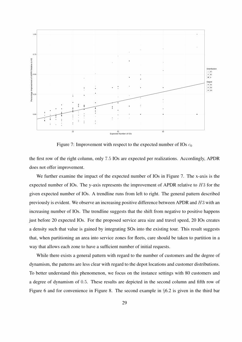
Figure 7: Improvement with respect to the expected number of IOs c0

the first row of the right column, only 7.5 IOs are expected per realizations. Accordingly, APDR

does not offer improvement.

We further examine the impact of the expected number of IOs in Figure 7. The x-axis is the

expected number of IOs. The y-axis represents the improvement of APDR relative to H3 for the

given expected number of IOs. A trendline runs from left to right. The general pattern described

previously is evident. We observe an increasing positive difference between APDR andH3 with an

increasing number of IOs. The trendline suggests that the shift from negative to positive happens

just before 20 expected IOs. For the proposed service area size and travel speed, 20 IOs creates

a density such that value is gained by integrating SOs into the existing tour. This result suggests

that, when partitioning an area into service zones for fleets, care should be taken to partition in a

way that allows each zone to have a sufficient number of initial requests.

While there exists a general pattern with regard to the number of customers and the degree of

dynamism, the patterns are less clear with regard to the depot locations and customer distributions.

To better understand this phenomenon, we focus on the instance settings with 80 customers and

a degree of dynamism of 0.5. These results are depicted in the second column and fifth row of

Figure 6 and for convenience in Figure 8. The second example in §6.2 is given in the third bar

29

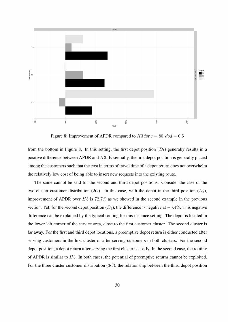
DOD: 50

2C

3C

U

Custom

ers: 80

−25

%

0% 25%

50%

75%

100%

value

Dis

trib

utio

n DepotD1

D2

D3

Figure 8: Improvement of APDR compared to H3 for c = 80, dod = 0.5

from the bottom in Figure 8. In this setting, the first depot position (D1) generally results in a

positive difference between APDR and H3. Essentially, the first depot position is generally placed

among the customers such that the cost in terms of travel time of a depot return does not overwhelm

the relatively low cost of being able to insert new requests into the existing route.

The same cannot be said for the second and third depot positions. Consider the case of the

two cluster customer distribution (2C). In this case, with the depot in the third position (D3),

improvement of APDR over H3 is 72.7% as we showed in the second example in the previous

section. Yet, for the second depot position (D2), the difference is negative at−5.4%. This negative

difference can be explained by the typical routing for this instance setting. The depot is located in

the lower left corner of the service area, close to the first customer cluster. The second cluster is

far away. For the first and third depot locations, a preemptive depot return is either conducted after

serving customers in the first cluster or after serving customers in both clusters. For the second

depot position, a depot return after serving the first cluster is costly. In the second case, the routing

of APDR is similar to H3. In both cases, the potential of preemptive returns cannot be exploited.

For the three cluster customer distribution (3C), the relationship between the third depot position

30

experiences a negative difference and the second a positive difference. The difference results from

the relative cost of a return to the depot and a sufficient passage of time to accumulate SOs. In

essence, the depot location significantly impacts the potential of preemptive depot returns. The

results related to the 2C and 3C depot locations suggest that the decision of whether or not to

implement preemptive depot returns should be made for a vehicle based on the characteristics of

the service area being served by the vehicle.

7 Conclusion and Outlook

In this paper, we explore preemptive depot returns for the SDPD, a dynamic one-to-many pickup

and delivery problem induced by a same-day delivery application. We present an anticipatory

assignment and routing policy APDR. APDR is based on approximate dynamic programming and

enables explicit decisions about preemptive depot returns. In extensive computational studies, we

show that preemptive depot returns and our APDR approach in particularly increase the number of

deliveries per workday. Our analysis of our computational tests that ADPR is most beneficial when

density is high enough to reduce the relative marginal cost of serving a new request. Our results

also show that preemptive returns are most effective when the returns occur late enough in the

horizon that enough time passed so that a sufficient number of stochastic customer requests have

accumulated but not so much that there is no longer time to serve the new requests. If considering

a fleet of vehicles, these results provide guidelines for how the delivery area can be partitioned so

that the delivery vehicles can benefit from preemptive depot returns.

There are a number of directions for future research. First, the presented state-space aggrega-

tion does not explicitly account for spatial information. Notably, the routing behavior presented

in Figure 5 is not achieved for every realization. For some realizations, APDR results in the same

routing as P2 and P1. Such cases might benefit from the inclusion of spatial information in the

aggregation scheme. The authors are not aware of any fully offline approximate dynamic pro-

gramming approach, whether it state-space aggregation or value-function approximation, that has

successfully incorporated spatial information in the routing of vehicles.

A second area of future research might consider a fleet of vehicles that are not constrained by

delivery zones. As noted previously, our second and third depot positions can represent the position

31

of a depot for a fleet divided into delivery zones, but we do not explicitly consider integrated

decision making for a fleet. In the integrated fleet context, the approach presented in this paper,

particularly the state space aggregation would require alteration to consider the impact of multiple,

interacting vehicles.

A third area of future research would be variants of the problem that incorporate third party

and/or crowdsourced vehicles. In addition, APDR may be extended to communicate potential de-

livery times to the customers. These could be also used for pricing decisions for time windows.

Finally, the general area of same-day delivery additionally offers challenges on strategic and tacti-

cal decision levels. For instance, future research might consider suitable depot locations as well as

the flow of inventory between depots.

References

Addady, Michal. 2015. Macy’s is taking on Amazon with same-day delivery in 17 cities. Fortune Avail-

able from http://fortune.com/2015/08/04/macys--amazon--delivery/, accessed

on July 14, 2016.

Azi, Nabila, Michel Gendreau, Jean-Yves Potvin. 2012. A dynamic vehicle routing problem with multiple

delivery routes. Annals of Operations Research 199(1) 103–112.

Barto, Andrew G. 1998. Reinforcement learning: An introduction. MIT press.

Ben-Shabat, Hana, Parvaneh Nilforoushan, Christine Moriarty, Mike nad Yuen. 2015. The 2015 Global

Retail E-Commerce Index: Global retail e-commerce keeps on clicking. Tech. rep., ATKearny,

Available from https://www.atkearney.com/documents/10192/5691153/Global+

Retail+E-Commerce+Keeps+On+Clicking.pdf/abe38776-2669-47ba-9387-

5d1653e40409, accessed on July 14, 2016.

Berbeglia, Gerardo, Jean-Francois Cordeau, Gilbert Laporte. 2010. Dynamic pickup and delivery problems.

European Journal of Operational Research 202(1) 8 – 15.

Bertsimas, Dimitris J, P. Chervi, M. Peterson. 1996. Computational approaches to stochastic vehicle routing

problems. Transportation Science 29(4) 342–352.

Ehmke, Jan Fabian, Ann Melissa Campbell. 2014. Customer acceptance mechanisms for home deliveries in

metropolitan areas. European Journal of Operational Research 233(1) 193–207.

32

Ehmke, Jan Fabian, Ann Melissa Campbell, Timothy L Urban. 2015. Ensuring service levels in routing

problems with time windows and stochastic travel times. European Journal of Operational Research

240(2) 539–550.

Fedde, Corey. 2016. Amazon expands same-day delivery – for some. Christian Science

Monitor Available from http://www.csmonitor.com/Business/2016/0407/Amazon-

-expands--same--day--delivery--for--some, accessed on July 14, 2016.

Ghiani, G., E. Manni, B. W. Thomas. 2011. A Comparison of Anticipatory Algorithms for

the Dynamic and Stochastic Traveling Salesman Problem. Transportation Science 46(3) 374–

387. doi:10.1287/trsc.1110.0374. URL http://transci.journal.informs.org/cgi/doi/

10.1287/trsc.1110.0374.

Goodson, Justin C, Barrett W Thomas, Jeffrey W Ohlmann. 2016a. Restocking-based rollout policies for

the vehicle routing problem with stochastic demand and duration limits. Transportation Science 50(2)

591 – 607.

Goodson, Justin C, Barrett W Thomas, Jeffrey W Ohlmann. 2016b. A rollout algorithm framework

for heuristic solutions to finite-horizon stochastic dynamic programs,. Available from http://

www.slu.edu/˜goodson/papers/GoodsonRolloutFramework.pdf.

Kall, P, SW Wallace. 1994. Stochastic Programming. John Wiley & Sons.

Klapp, Mathias, Alan L Erera, Alejandro Toriello. 2015. The one-dimensional dynamic dispatch waves

problem. Tech. rep., Georgia Institute of Technology.

Kumar, Kavita. 2016. Best buy rolls out same-day delivery in 13 markets. Minneapolis Star Tribune Avail-

able from http://www.startribune.com/best--buy--rolls--out--same--day-

-delivery--in--a--dozen--markets/374807051/, accessed on July 14, 2016.

Larsen, Allan, OBGD Madsen, Marius Solomon. 2002. Partially dynamic vehicle routing-models and algo-

rithms. Journal of the Operational Research Society 637–646.

Meisel, Stephan. 2011. Anticipatory Optimization for Dynamic Decision Making, Operations Re-

search/Computer Science Interfaces Series, vol. 51. Springer Science+Business Media, New York.

Mes, Martijn, Matthieu van der Heijden, Peter Schuur. 2010. Look-ahead strategies for dynamic pickup and

delivery problems. OR spectrum 32(2) 395–421.

Mitrovic-Minic, Snezana, Gilbert Laporte. 2004. Waiting strategies for the dynamic pickup and delivery

problem with time windows. Transportation Research Part B: Methodological 38(7) 635–655.

33

Powell, W. 2011. Approximate Dynamic Programming: Solving the Curses of Dimensionality. 2nd ed. John

Wiley and Sons, Hoboken, NJ, USA.

Pureza, Vitoria, Gilbert Laporte. 2008. Waiting and buffering strategies for the dynamic pickup and delivery

problem with time windows. INFOR: Information Systems and Operational Research 46(3) 165–176.

Rosenkrantz, Daniel J, Richard Edwin Stearns, PM Lewis. 1974. Approximate algorithms for the traveling

salesperson problem. Switching and Automata Theory, 1974., IEEE Conference Record of 15th Annual

Symposium on. IEEE, 33–42.

Saez, Doris, Cristian E Cortes, Alfredo Nunez. 2008. Hybrid adaptive predictive control for the multi-vehicle

dynamic pick-up and delivery problem based on genetic algorithms and fuzzy clustering. Computers

& Operations Research 35(11) 3412–3438.

Secomandi, Nicola. 2003. Analysis of a rollout approach to sequencing problems with stochastic routing

applications. Journal of Heuristics 9(4) 321–352.

Ulmer, Marlin W, Justin C Goodson, Dirk C Mattfeld, Marco Hennig. 2015. Offline-online approximate

dynamic programming for dynamic vehicle routing with stochastic requests. Tech. rep., Technische

Universitat Braunschweig, Germany.

Ulmer, Marlin W., Dirk C. Mattfeld, Felix Koster. 2016a. Budgeting time for dynamic vehicle routing with

stochastic customer requests. To appear in Transportation Science .

Ulmer, Marlin W, Dirk C Mattfeld, Ninja Soeffker. 2016b. Dynamic multi-period vehicle routing: approxi-

mate value iteration based on dynamic lookup tables. Tech. rep., Technische Universitat Braunschweig,

Germany.

Ulmer, Marlin W, Barrett W Thomas. 2016. Estimating arrival times for service vehicle routing with stochas-

tic and dynamic requests. Working Paper .

Voccia, Stacy A, Ann Melissa Campbell, Barrett W Thomas. 2015. The same-day delivery problem for

online purchases. Tech. rep., University of Iowa.

Yahoo! Finance. 2016. Increased value-added services expected to boost the same-day delivery market in

the US, says Technavio. Yahoo! Finance Available from http://finance.yahoo.com/news/

increased--value--added--services--expected--204000803.html, accessed on

July 14, 2016.

Yang, W., K. Mathur, R. Ballou. 2000. Stochastic vehicle routing problem with restocking. Transportation

Science 34(1) 99–112.

34

Appendix

In the Appendix, we present instance generation details, the PDR-algorithm as well as the results

and parameters for every instance setting.

A.1 Instance Generation Details

In the following, we describe how the realizations for the computational evaluation are generated.

The number of customers and the order times for a realization are generated by a Poisson process

P. With c0 the expected number of IOs, the number of IOs is generated by P(c0). The spatial

and temporal probability distribution for order times and locations is divided into two independent

probability distributions. The times of SO occurrences are (discretely) uniformly distributed t ∼

UZ[1, tmax − 1]. Customer locations f(C) ∈ A are realizations f ∼ F of the spatial probability

distribution F : A → [0, 1]. A realization of the order time is again conducted by a Poisson

process P for every minute 0 < t < tmax. Given two points of time 0 < tj < th < tmax, this results

in an expected number of customers of cthtj = Eω∈Ω

∣∣Cωi ∈ Cω+ : tj < ti ≤ th

∣∣ ordering in times

tj < ti ≤ th as described in Equation A1.

cth

tj = dod · c · th − tj

T − 2(A1)

35

A.2 Preemptive Depot Returns: Algorithm

This section presents a detailed algorithm for the PDR routing heuristic that was described in §4.3.

Algorithm 2: Preemptive Depot ReturnsInput : Tour θk = (Pk, Cl, . . . , Cl,D, Cn, Cl, Cn, . . . , Cl,D), New orders Cr = C1

r , . . . , Chr

Output : New tour θ

1 θ ← ∅

2 // Remove Depot

3 for all θik, i = 1, . . . , |θk| − 1 do

4 if θik 6= D then θ ← θ ∪ θik

5 end

6 θ ← θ ∪ D

7 // Integrate Orders

8 while Cr 6= ∅ do

9 δ ←M

10 for all Ci, θj , i = 1, . . . , |Cr|, j = 1, . . . , |θ| − 1 do

11 if d(θj , Ci) + d(Ci, θj+1)− d(θj , θj+1) ≤ δ then

12 C∗ ← Ci, θ∗ ← θj

13 δ ← d(θj , Ci) + d(Ci, θj+1)− d(θj , θj+1)

14 end

15 end

16 θ ← Insert(θ, θ∗, C∗), Cr ← Cr\C∗

17 end

18 // Integrate Depot

19 δ ←M , j ← 0

20 while θj /∈ Cn, Cr,D do

21 if d(θj ,D) + d(D, θj+1)− d(θj , θj+1) ≤ δ then

22 θ∗ ← θj , δ = d(θj ,D) + d(D, θj+1)− d(θj , θj+1)

23 end

24 j ← j + 1

25 end

26 θ ← Insert(θ, θ∗,D)

27 return θ

Detailed Results

In this section, we present the detailed results for the computational experiments discussed in

§6. The first table presents the average number of assignments for APDR and each benchmark

over all realizations for each instance setting. The second table presents the average number of

depot returns, the average time required for a depot return, and the initial free time budget over all

36

realizations for each instance setting for APDR.

37

Table A1: Average Number of Assignments

Distribution U 2C 3C

dod Depot c APDR P2 P1 H3 H2 H1 APDR P2 P1 H3 H2 H1 APDR P2 P1 H3 H2 H1

0.25 D1 30 2.7 2.7 2.7 2.4 2.2 2.3 4.6 4.6 4.6 4.5 4.5 4.5 4.5 4.5 4.5 4.6 4.5 4.5

0.5 D1 30 6.4 6.3 6.1 6 5.5 5.6 8.6 8.6 8.7 8.5 8.5 8.5 8.3 8.2 8.3 8.3 8.3 8.3

0.75 D1 30 10.6 10.5 10.1 10.3 10.2 9.7 12.4 12.3 12.5 12.3 12.1 12.1 12.2 12.2 12.2 12.4 12.2 12.2

0.25 D2 30 1.1 1 1.1 1 0.9 1 3.2 3.1 3.1 3.3 3.3 3.3 2.6 2.5 2.6 2.8 2.6 2.8

0.5 D2 30 3.8 3.5 3.6 3.8 3.3 3.5 6.5 6.3 6.3 6.9 6.8 6.7 5.6 5.3 5.4 6.4 6.3 6.1

0.75 D2 30 7.3 6.9 7 7.8 7.7 7.2 10 9.6 9.8 10.6 10.4 10.5 9 8.8 8.8 9.7 9.6 9.5

0.25 D3 30 1.1 1.1 1.1 1 0.9 1 2.2 2.2 2.2 2.2 2 2.1 3.2 3.1 3.2 3.5 3.4 3.4

0.5 D3 30 3.8 3.5 3.6 3.8 3.3 3.5 4.7 4.5 4.6 5.3 5.2 5.1 6.4 6 6.1 6.9 6.8 6.7

0.75 D3 30 7.3 7 7 7.8 7.7 7.2 8.1 7.9 8 8.8 8.8 8.6 10.1 9.6 9.6 10.6 10.2 10.3

0.25 D1 40 1.5 1.4 1.4 1.1 1 1 4.9 4.8 4.9 4.8 4.6 4.7 4.4 4.4 4.4 4.4 3.8 4.3

0.5 D1 40 5.9 5.6 5.4 5 4.4 4.3 9.6 9.3 9.6 9.8 9.5 9.6 9 8.8 8.9 9.3 8.8 9

0.75 D1 40 11.5 11.2 10.6 10.9 10.6 9.5 14.6 14.4 14.8 14.7 14 14.2 14.1 13.8 13.9 14.3 13.9 13.9

0.25 D2 40 0.4 0.4 0.4 0.4 0.4 0.4 3.2 3.1 3.1 3.3 3.2 3.2 2.2 2.1 2.2 2.2 1.9 2.1

0.5 D2 40 3 2.6 2.8 2.8 2.3 2.5 7.3 6.7 6.9 7.8 7.6 7 5.6 5 5.4 6.3 5.8 5.6

0.75 D2 40 7.7 7.1 7.2 8.1 7.7 6.6 11.8 10.9 11.3 12.6 12.4 12.3 10.2 9.7 9.9 11.5 11.4 10.7

0.25 D3 40 0.4 0.4 0.4 0.3 0.3 0.3 1.7 1.6 1.7 1.1 1 1.1 2.8 2.5 2.7 3.1 2.5 2.9

0.5 D3 40 2.9 2.6 2.8 2.8 2.3 2.5 5.2 4.9 4.9 4.9 4.6 4.5 6.8 6 6.3 7.6 7.3 6.7

0.75 D3 40 7.8 7.3 7.3 8.3 7.9 6.7 9.2 8.8 8.8 10.2 10 9.3 11.7 10.7 10.9 12.5 12.1 11.6

0.25 D1 50 0.4 0.4 0.4 0.3 0.3 0.3 4.6 4.4 4.5 4.2 3.4 4 3.7 3.6 3.6 3.2 2.6 3

0.5 D1 50 4.6 4.2 3.9 3.5 3 2.8 10 9.6 9.9 10.1 9.3 9.3 9.3 8.9 8.9 9.3 7.9 8.3

0.75 D1 50 12.2 11.7 10.8 11.4 10.5 8.9 16.4 15.9 16.3 16.3 15.8 15.8 15.3 14.8 15 15.7 15.4 14.8

0.25 D2 50 0.1 0.1 0.1 0.1 0.1 0.1 2.7 2.4 2.6 2.9 2.2 2.8 1.3 1.1 1.2 1.2 1 1.1

0.5 D2 50 1.8 1.7 1.7 1.7 1.4 1.5 7.4 6.4 6.7 7.8 7.6 6.5 5.4 4.6 5.1 5.5 4.7 4.5

0.75 D2 50 7.8 7.2 7.3 8.1 7.5 6 13.2 11.7 12.4 13.7 13.4 12.7 11.2 10.4 10.7 12.6 12.5 10.7

0.25 D3 50 0.1 0.1 0.1 0.1 0.1 0.1 0.8 0.7 0.8 0.3 0.2 0.3 2 1.6 1.8 2.1 1.5 2

0.5 D3 50 1.8 1.6 1.7 1.7 1.4 1.5 4.9 4.4 4.5 3.4 3.1 3.1 6.7 5.4 5.8 7.4 6.2 5.8

0.75 D3 50 8 7.4 7.3 8.1 7.4 5.9 10 9.6 9.4 10.6 10.3 8.6 12.7 10.9 11.5 13.5 13.3 11.5

0.25 D1 60 0.1 0.1 0.1 0 0 0 3.9 3.8 3.8 3 2.2 2.8 2.5 2.3 2.3 1.6 1.3 1.6

0.5 D1 60 2.6 2.3 2.3 1.8 1.6 1.5 10 9.6 9.6 9.8 8.4 8.3 9.1 8.5 8.5 8.4 6.3 6.9

0.75 D1 60 12.2 11.4 10.1 10.7 9.3 7.6 17.7 17 17.3 17.6 17.1 16.9 16.4 15.7 15.7 16.7 16.2 15

0.25 D2 60 0 0 0 0 0 0 1.7 1.4 1.6 1.8 1.3 1.8 0.6 0.5 0.6 0.5 0.4 0.5

0.5 D2 60 1 0.9 0.9 0.9 0.8 0.8 7.3 5.9 6.4 7.9 6.6 6.4 4.6 3.8 4.2 4.3 3.2 3.5

0.75 D2 60 7.6 6.9 6.8 7.5 6.6 5.1 14.3 12.3 13.1 14.7 14.4 11.8 11.4 10.4 11 12.7 12.2 9.5

0.25 D3 60 0 0 0 0 0 0 0.2 0.1 0.2 0 0 0 0.9 0.7 0.8 0.9 0.6 0.9

0.5 D3 60 0.8 0.7 0.8 0.7 0.6 0.7 3.9 3.3 3.5 1.9 1.6 1.7 6 4.4 4.9 6.7 4.3 5.2

0.75 D3 60 7.6 6.9 6.9 7.5 6.3 5.2 10.7 10.2 10.2 10.3 10 7.5 13.5 11.4 11.9 14.4 14.2 10.9

0.25 D1 80 0 0 0 0 0 0 1.4 1.3 1.3 0.5 0.4 0.5 0.3 0.3 0.3 0.1 0.1 0.1

0.5 D1 80 0.4 0.4 0.4 0.3 0.3 0.2 9.2 8.5 7.9 7.2 4.8 5.2 6.4 5.4 5.4 4.4 3 3.4

0.75 D1 80 11.2 10.1 8.5 8.7 7.2 5.6 19.3 18 17.9 18.7 17.6 15.7 17.7 16.5 16.1 17.2 15.8 12.7

0.25 D2 80 0 0 0 0 0 0 0.2 0.2 0.2 0.2 0.1 0.2 0 0 0 0 0 0

0.5 D2 80 0.1 0.1 0.1 0.1 0.1 0.1 4.8 3.6 4.1 5.1 3.1 4.4 2.1 1.9 2 1.8 1.2 1.6

0.75 D2 80 5.7 5.1 5.1 5.3 4.1 3.8 14.9 12.5 13.5 15.8 15.5 9.6 11.3 10.3 10.8 11.4 10.8 7.1

0.25 D3 80 0 0 0 0 0 0 0 0 0 0 0 0 0 0 0 0 0 0

0.5 D3 80 0.1 0.1 0.1 0.1 0.1 0.1 1 0.9 0.9 0.3 0.2 0.3 2.9 2.3 2.5 2.9 1.7 2.4

0.75 D3 80 5.5 4.9 4.9 5.1 3.9 3.6 11.3 10.5 10.1 8.5 7.8 5.8 13.8 11.2 11.9 15.3 14.5 8.8

0.25 D1 100 0 0 0 0 0 0 0.1 0.1 0.1 0 0 0 0 0 0 0 0 0

0.5 D1 100 0 0 0 0 0 0 6.2 5.5 4.9 3.1 2 2.4 2.8 2.3 2.4 1.4 1.1 1.2

0.75 D1 100 7.9 7 5.7 5.3 4.6 3.5 20.2 18.3 17.2 18.4 17.4 12 17.8 15.6 14.9 15.7 14.1 9.8

0.25 D2 100 0 0 0 0 0 0 0 0 0 0 0 0 0 0 0 0 0 0

0.5 D2 100 0 0 0 0 0 0 1.8 1.5 1.7 1.6 1.1 1.4 0.4 0.4 0.4 0.4 0.3 0.3

0.75 D2 100 3.5 3 3 3.1 2.4 2.3 14.2 11.9 12.9 15.7 14.3 8.3 10.4 9.4 9.9 9.7 8.7 5.6

0.25 D3 100 0 0 0 0 0 0 0 0 0 0 0 0 0 0 0 0 0 0

0.5 D3 100 0 0 0 0 0 0 0.1 0.1 0.1 0 0 0 0.6 0.5 0.6 0.5 0.4 0.5

0.75 D3 100 3.6 3.1 3.2 3.2 2.4 2.4 10.4 9.2 8.5 5.7 5.3 4.2 12.3 9.9 10.7 13.4 11.3 7

38

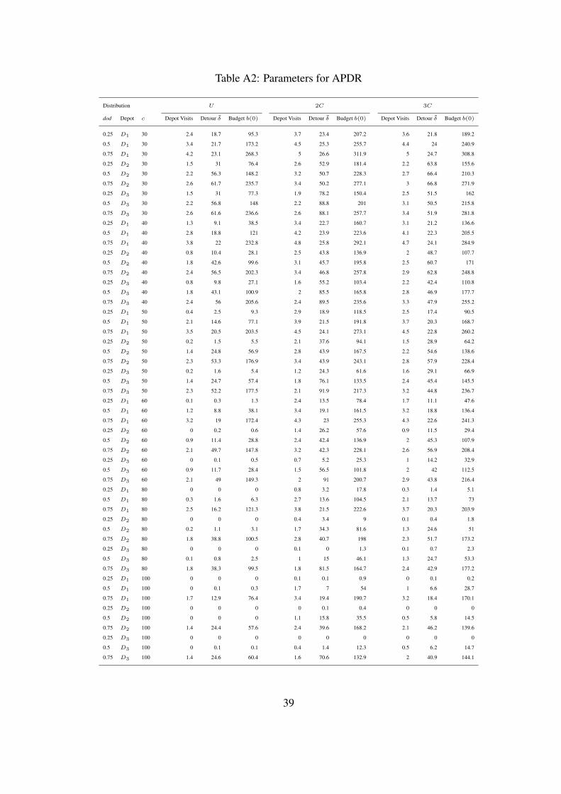
Table A2: Parameters for APDR

Distribution U 2C 3C

dod Depot c Depot Visits Detour δ Budget b(0) Depot Visits Detour δ Budget b(0) Depot Visits Detour δ Budget b(0)

0.25 D1 30 2.4 18.7 95.3 3.7 23.4 207.2 3.6 21.8 189.2

0.5 D1 30 3.4 21.7 173.2 4.5 25.3 255.7 4.4 24 240.9

0.75 D1 30 4.2 23.1 268.3 5 26.6 311.9 5 24.7 308.8

0.25 D2 30 1.5 31 76.4 2.6 52.9 181.4 2.2 63.8 155.6

0.5 D2 30 2.2 56.3 148.2 3.2 50.7 228.3 2.7 66.4 210.3

0.75 D2 30 2.6 61.7 235.7 3.4 50.2 277.1 3 66.8 271.9

0.25 D3 30 1.5 31 77.3 1.9 78.2 150.4 2.5 51.5 162

0.5 D3 30 2.2 56.8 148 2.2 88.8 201 3.1 50.5 215.8

0.75 D3 30 2.6 61.6 236.6 2.6 88.1 257.7 3.4 51.9 281.8

0.25 D1 40 1.3 9.1 38.5 3.4 22.7 160.7 3.1 21.2 136.6

0.5 D1 40 2.8 18.8 121 4.2 23.9 223.6 4.1 22.3 205.5

0.75 D1 40 3.8 22 232.8 4.8 25.8 292.1 4.7 24.1 284.9

0.25 D2 40 0.8 10.4 28.1 2.5 43.8 136.9 2 48.7 107.7

0.5 D2 40 1.8 42.6 99.6 3.1 45.7 195.8 2.5 60.7 171

0.75 D2 40 2.4 56.5 202.3 3.4 46.8 257.8 2.9 62.8 248.8

0.25 D3 40 0.8 9.8 27.1 1.6 55.2 103.4 2.2 42.4 110.8

0.5 D3 40 1.8 43.1 100.9 2 85.5 165.8 2.8 46.9 177.7

0.75 D3 40 2.4 56 205.6 2.4 89.5 235.6 3.3 47.9 255.2

0.25 D1 50 0.4 2.5 9.3 2.9 18.9 118.5 2.5 17.4 90.5

0.5 D1 50 2.1 14.6 77.1 3.9 21.5 191.8 3.7 20.3 168.7

0.75 D1 50 3.5 20.5 203.5 4.5 24.1 273.1 4.5 22.8 260.2

0.25 D2 50 0.2 1.5 5.5 2.1 37.6 94.1 1.5 28.9 64.2

0.5 D2 50 1.4 24.8 56.9 2.8 43.9 167.5 2.2 54.6 138.6

0.75 D2 50 2.3 53.3 176.9 3.4 43.9 243.1 2.8 57.9 228.4

0.25 D3 50 0.2 1.6 5.4 1.2 24.3 61.6 1.6 29.1 66.9

0.5 D3 50 1.4 24.7 57.4 1.8 76.1 133.5 2.4 45.4 145.5

0.75 D3 50 2.3 52.2 177.5 2.1 91.9 217.3 3.2 44.8 236.7

0.25 D1 60 0.1 0.3 1.3 2.4 13.5 78.4 1.7 11.1 47.6

0.5 D1 60 1.2 8.8 38.1 3.4 19.1 161.5 3.2 18.8 136.4

0.75 D1 60 3.2 19 172.4 4.3 23 255.3 4.3 22.6 241.3

0.25 D2 60 0 0.2 0.6 1.4 26.2 57.6 0.9 11.5 29.4

0.5 D2 60 0.9 11.4 28.8 2.4 42.4 136.9 2 45.3 107.9

0.75 D2 60 2.1 49.7 147.8 3.2 42.3 228.1 2.6 56.9 208.4

0.25 D3 60 0 0.1 0.5 0.7 5.2 25.3 1 14.2 32.9

0.5 D3 60 0.9 11.7 28.4 1.5 56.5 101.8 2 42 112.5

0.75 D3 60 2.1 49 149.3 2 91 200.7 2.9 43.8 216.4

0.25 D1 80 0 0 0 0.8 3.2 17.8 0.3 1.4 5.1

0.5 D1 80 0.3 1.6 6.3 2.7 13.6 104.5 2.1 13.7 73

0.75 D1 80 2.5 16.2 121.3 3.8 21.5 222.6 3.7 20.3 203.9

0.25 D2 80 0 0 0 0.4 3.4 9 0.1 0.4 1.8

0.5 D2 80 0.2 1.1 3.1 1.7 34.3 81.6 1.3 24.6 51

0.75 D2 80 1.8 38.8 100.5 2.8 40.7 198 2.3 51.7 173.2

0.25 D3 80 0 0 0 0.1 0 1.3 0.1 0.7 2.3

0.5 D3 80 0.1 0.8 2.5 1 15 46.1 1.3 24.7 53.3

0.75 D3 80 1.8 38.3 99.5 1.8 81.5 164.7 2.4 42.9 177.2

0.25 D1 100 0 0 0 0.1 0.1 0.9 0 0.1 0.2

0.5 D1 100 0 0.1 0.3 1.7 7 54 1 6.6 28.7

0.75 D1 100 1.7 12.9 76.4 3.4 19.4 190.7 3.2 18.4 170.1

0.25 D2 100 0 0 0 0 0.1 0.4 0 0 0

0.5 D2 100 0 0 0 1.1 15.8 35.5 0.5 5.8 14.5

0.75 D2 100 1.4 24.4 57.6 2.4 39.6 168.2 2.1 46.2 139.6

0.25 D3 100 0 0 0 0 0 0 0 0 0

0.5 D3 100 0 0.1 0.1 0.4 1.4 12.3 0.5 6.2 14.7

0.75 D3 100 1.4 24.6 60.4 1.6 70.6 132.9 2 40.9 144.1

39