Applied Mathematics and Computation 218 (2011) 3905–3917

Contents lists available at SciVerse ScienceDirect

Applied Mathematics and Computation

journal homepage: www.elsevier .com/ locate/amc

Predictor–corrector pseudospectral methods for stochastic partialdifferential equations with additive white noise

Rafael GallegoDepartamento de Matemáticas, Universidad de Oviedo, Spain

a r t i c l e i n f o

Keywords:Pseudospectral methodsStochastic partial differential equationsStochastic PDEsGrowth modelsFourier transform

0096-3003/$ - see front matter � 2011 Elsevier Incdoi:10.1016/j.amc.2011.09.038

E-mail address: rgallego@uniovi.es

a b s t r a c t

Commonly used finite-difference numerical schemes show some deficiencies in the inte-gration of certain types of stochastic partial differential equations with additive whitenoise. In this paper efficient predictor–corrector spectral schemes to integrate these equa-tions are discussed. They are all based on the discretization of the system in Fourier space.The nonlinear terms are treated using a pseudospectral approach so as to speed up thecomputations without a significant loss of accuracy. The proposed schemes are appliedto solve, both in one and two spatial dimensions, two paradigmatic continuum models aris-ing in the context of nonequilibrium dynamics of growing interfaces: the Kardar–Parisi–Zhang and Lai–Das Sarma–Villain equations. Numerical results about the Lai–Das Sar-ma–Villain equation in two spatial dimensions have not been previously reported in theliterature.

� 2011 Elsevier Inc. All rights reserved.

1. Introduction

Numerical integration is often a direct and convenient way to study the behavior of partial differential equations (PDEs).Regarding stochastic partial differential equations (SPDEs), finite-difference methods have been traditionally used. Spectralmethods, on the other hand, are frequently used to integrate PDEs arising in Fluid Dynamics, but only recently they havebeen considered for SPDEs [1–3]. For certain types of equations, spectral schemes are more reliable and accurate thanfinite-difference based algorithms since the latter may give rise to numerical artifacts due to discretization effects. Theseartifacts may lead to a wrong interpretation of the results of numerical simulations. In [4,5] it is shown by means of numer-ical simulations that discretized versions of commonly studied nonlinear growth equations exhibit an instability in the sensethat single pillars (grooves) become unstable when their height (depth) exceeds a critical value. In some cases these insta-bilities are not present in the corresponding continuum equations, indicating that the behavior of the discretized versions isindeed different from their continuum counterparts. Moreover, it has been proved that results of numerical simulations candepend on the particular discretization used to evaluate the partial derivatives [6]. This unwanted feature is not present inspectral methods inasmuch as derivatives are computed in Fourier space using the values of the field at all points. On theother hand, spectral methods may be rather time-consuming. In order to speed up the computation, a pseudospectral ap-proach is commonly used to deal with the nonlinear terms.

The problem of kinetic surface roughening has attracted much attention in the last years owing to its many importantapplications as molecular beam epitaxy, fluid flow in porous media, fracture cracks, etc. Theoretical approaches make useof both discrete atomistic simulations and stochastic continuum equations for the evolution of the coarse-grained surfaceheight h(x, t). Growth models are often classified into universality classes according to the values of certain critical exponentsthat characterize the growth process and that do not depend on the microscopic details of the system under study. Although

. All rights reserved.

3906 R. Gallego / Applied Mathematics and Computation 218 (2011) 3905–3917

a perturbative renormalization approach provides the critical exponents of a particular growth model, often these are ob-tained with an approximation valid up to a certain order, and a great algebraic effort is required to improve this approxima-tion. This makes numerical simulations of growth models a useful and convenient tool as the most reliable source of precisevalues for the critical exponents.

Universality classes are generically represented by SPDEs. The Kardar–Parisi–Zhang (KPZ) [7] and the Lai–Das Sarma–Vil-lain equations (LDV) [8–10] are examples of continuum nonlinear growth models. Both equations can be derived on the basisof physical and symmetry principles. The KPZ equation is a Langevin type equation that was first introduced to give a hydro-dynamic description of ballistic deposition growth far from equilibrium. If h(x, t) is the local height on a d-dimensional sub-strate, the KPZ equation reads:

@thðx; tÞ ¼ mr2hþ kðrhÞ2 þ nðx; tÞ: ð1Þ

The stochastic term n(x, t) represents the influx of atoms on the surface. It is a Gaussian noise with mean zero and uncorre-lated in space and time, that is,

hnðx; tÞi ¼ 0; hnðx; tÞnðx0; t0Þi ¼ 2Dddðx� x0Þdðt � t0Þ:

The LDV equation describes the long-wavelength fluctuations of crystal growth from atom beams in the absence of diffusionbias:

@thðx; tÞ ¼ �Kr4hþ kr2ðrhÞ2 þ nðx; tÞ: ð2Þ

Eqs. (1) and (2) can be transformed by adequate rescaling of the parameters into equations with only one independent con-trol parameter so that they can be rewritten in dimensionless form:

@thðx; tÞ ¼ r2hþ gðrhÞ2 þ gðx; tÞ; g ¼ kffiffiffiffiffiffiffiffiffiffiffiffiffiffi2D=m3

qðKPZÞ; ð3Þ

@thðx; tÞ ¼ �r4hþ gr2ðrhÞ2 þ gðx; tÞ; g ¼ kffiffiffiffiffiffiffiffiffiffiffiffiffiffi2D=K3

qðLDVÞ: ð4Þ

Now, g(x, t) is a Gaussian noise with mean zero and correlations given by:

hgðx; tÞgðx0; t0Þi ¼ ddðx� x0Þdðt � t0Þ:

In this work we present two predictor–corrector numerical schemes adapted for the integration of SPDEs with additive whitenoise. In addition, two other numerical schemes described in previous works are considered for comparison. The proposedschemes are based on the discretization of the system in Fourier space and they are applied to the numerical integration,both in one (1D) and two (2D) spatial dimensions, of Eqs. (3) and (4). As far as I know no results of the numerical integrationof the 2D LDV equation have been appeared yet in the literature. The stability of the algorithms is studied by measuring theprobability for a numerical overflow to occur in the simulations. This probability is related to the maximum time up to whichthe equations can be integrated.

The text is organized as follows. Section 2 is devoted to the description of the several numerical schemes. In Section 3 theprevious schemes are applied to the integration of the KPZ and LDV equations in 1D and 2D. Several critical exponents arecomputed, and the numerical stability of the algorithms and the existence of multiscaling are studied. Finally, concludingremarks are provided in Section 4.

2. Numerical schemes

In this section two numerical schemes to integrate SPDEs with additive white noise are presented. They are predictor–corrector spectral methods based on the discretization of the system in momentum space. Two other spectral methods in-cluded in previous works are also considered for comparison.

The numerical schemes to be considered are valid to integrate SPDEs of the form:

@thðx; tÞ ¼ L½h�ðx; tÞ þU½h�ðx; tÞ þ nðx; tÞ; ð5Þ

where L½h� is a linear functional of the field h, U[h] is another functional comprising the nonlinear terms and n(x, t) is a whitenoise in space and time:

hnðx; tÞi ¼ 0; hnðx; tÞnðx0; t0Þi ¼ 2Dddðx� x0Þdðt � t0Þ:

The explicit expressions of the functionals L½h� and U[h] for Eqs. (3) and (4) are:

KPZL½h�ðx; tÞ ¼ r2h

U½h�ðx; tÞ ¼ gðrhÞ2

(LDV

L½h�ðx; tÞ ¼ �r4h

U½h�ðx; tÞ ¼ gr2ðrhÞ2

(

Without loss of generality, a d-dimensional lattice of lateral size L with uniform spacing Dx in each direction is consid-ered. The field h is assumed to satisfy periodic boundary conditions in the multidimensional interval I = [0,L]d. The positions

R. Gallego / Applied Mathematics and Computation 218 (2011) 3905–3917 3907

of the nodes in the lattice are given by xj = Dx(j1, j2, . . . , jd), 0 6 ji 6 N � 1, 1 6 i 6 d, where N = (Dx)�1L is the lattice size in eachdirection.

In order to construct a spectral method, the field h(x, t) is represented as a truncated Fourier series:

hNðx; tÞ ¼Xk2CN

~hkðtÞeiqx; q ¼ 2pL

k;

where CN = {(k1,k2, . . . ,kd)/�N/2 6 ki 6 N/2 � 1,1 6 i 6 d} and the ~hkðtÞ’s are the Fourier coefficients of h, given by

~hkðtÞ ¼1

Ld

ZI

dxhðx; tÞe�iqx:

The noise term is also replaced by its expansion nN in Fourier modes. In the limit N ?1, the usual Fourier series is recovered.Finally, Eq. (5) is written in Fourier space as follows:

d~hkðtÞdt

¼ xk~hkðtÞ þ eUkðtÞ þ ~nkðtÞ; k 2 CN : ð6Þ

The quantity xk is the so-called linear dispersion relation, and comes from the Fourier transform of the linear part of theequation. It is xk = �q2 for the KPZ model and xk = �q4 for the LDV model. On the other hand, the eUkðtÞ’s are the Fouriermodes of the nonlinear terms. Let us find the correlations of the stochastic variables ~nkðtÞ. We have that:

~nkðtÞ ¼1

Ld

ZI

dxnðx; tÞe�iqx; h~nkðtÞi ¼ 0:

Then:

h~nkðtÞ~nk0 ðt0Þi ¼1

L2d

ZI

dxdye�iðqxþq0yÞhnðx; tÞnðy; t0Þi ¼ 2D

L2ddðt � t0Þ

ZI

dxe�i2pL ðkþk0Þx:

Now, using the equality

ZI

dxe�i2pL kx ¼ Lddk;0;

we get

h~nkðtÞ~nk0 ðt0Þi ¼2D

Lddðt � t0Þdk;�k0 :

As discussed in [2], Eq. (6) is difficult to treat numerically. The reason being that the Fourier coefficients are difficult andexpensive to compute, in special the eUkðtÞ’s associated to the nonlinear terms. The process of going from real space to Fourierspace and vice versa becomes a stiffly and a time-consuming task. Due to these reasons, the coefficients of the Fourier series~hk are approached with those of the discrete Fourier series that will be denoted by hk. The discrete Fourier coefficients dependonly on the value of the field at the nodes and they are given by (direct discrete Fourier transform):

hkðtÞ ¼ F½hj� ¼1

Nd

Xj

hjðtÞe�iqxj ; ð7Þ

where hj(t) = h(xj, t). There is also the inversion formula (inverse discrete Fourier transform):

hjðtÞ ¼ F�1½hk� ¼X

k

hkðtÞeiqxj :

Then instead of integrating the set of equations given by (6), the same set of equations with the Fourier coefficients re-placed by their discrete version is considered, so that

dhkðtÞdt

¼ xkhkðtÞ þ bUkðtÞ þ nkðtÞ: ð8Þ

The previous equation can be rewritten in differential form as follows:

dhkðtÞ ¼ aðhkðtÞÞdt þ b dcW kðtÞ; ð9Þ

where aðhkðtÞÞ :¼ xkhkðtÞ þ bUkðtÞ; dcW kðtÞ :¼ b�1nkðtÞdt, and b :¼ (2DL�d)1/2. Note that cW kðtÞ is a Wiener process whose timederivative turns out to be the noise term bnkðtÞ.

As for the noise term, we must act with caution when it is considered in a discretized space. Its discrete Fourier transformcannot be computed with Eq. (7) by just putting hj ? n(xj) since n(xj) is a Gaussian variable with infinite variance. The properresult is recovered by considering the relation between the Dirac delta and the Kronecker delta functions. In a space ofdimension d, this relation is d(xj) ? (Dx)�dd0n. Then, the discrete equivalent of the noise, n(xj,t) ? nj(t) has the followingcorrelations:

hnjðtÞi ¼ 0; hnjðtÞn0jðt0Þi ¼ 2DðDxÞ�ddj;j0dðt � t0Þ:

3908 R. Gallego / Applied Mathematics and Computation 218 (2011) 3905–3917

Now, the correlations of the variables nkðtÞ can be computed by using their definition:

hnkðtÞnk0 ðt0Þi ¼1

N2d

Xm;n

e�2pN iðmkþnk0ÞhnmðtÞnnðt0Þi ¼ 2DðDxÞ�ddðt � t0Þ

Xm

e�2pN imðkþk0 Þ ¼ b2dðt � t0Þdk;�k0 :

In order to integrate (8) it is useful to make the following change of variables based on the solution of the linear equation:

hkðtÞ ¼ exkt zkðtÞ þ bRkðtÞ; bRkðtÞ ¼ bexktZ t

0e�xksdcW kðsÞ: ð10Þ

Then, the variables zk satisfy the following set of ordinary differential equations:

dzkðtÞdt

¼ bUkðtÞe�xkt : ð11Þ

We now define the stochastic variables gkðtÞ that will be used afterwards:

gkðtÞ ¼ bRkðt þ DtÞ � bRkðtÞexkDt ¼ bexkðtþDtÞZ tþDt

te�xksdcW kðsÞ: ð12Þ

To compute the quantities gkðtÞ’s we need first to find out their correlations:

hgkðtÞgk0 ðt0Þi ¼ exkðtþDtÞexk0 ðt0þDtÞ

Z tþDt

tds1e�xks1

Z t0þDt

t0ds2e�xk0 s2 hnkðs1Þnk0 ðs2Þi:

If t – t0, then hgkðtÞgk0 ðt0Þi ¼ 0 since the intervals (t,t + Dt) and (t0, t0 + Dt) do not overlap. Otherwise, assuming thatx�k = xk, we have that:

hgkðtÞgk0 ðtÞi ¼ e2xkðtþDtÞb2dk;�k0

Z tþDt

tds1e�2xks1 ¼ e2xkDt � 1

xk

D

Lddk;�k0 :

In the computer, the numbers gk’s are obtained as follows:

gkðtÞ ¼ffiffiffiffiffiffiffiffiffiffiffiffiffiffiffiffiffiffiffiffiffiffiffiffiffiffiffiffiffiffiffiffiffiffie2xkDt � 1

xk

D

ðDxÞd

svkðtÞ; ð13Þ

where vkðtÞ are the discrete Fourier coefficients of a vector vn(t) of random Gaussian numbers of mean 0 and variance 1.

2.1. Numerical scheme PC2

The algorithm presented in this section is a stochastic variant of the so-called two-step method [11]. The starting point isthe following formal solution of Eq. (9):

hkðtÞ ¼ exkt hkðt0Þe�xkt0 þZ t

t0

dsbUkðsÞe�xks þ bZ t

t0

e�xksdcW kðsÞ� �

: ð14Þ

From (14), and with the substitutions t ? t + Dt, t0 ? t � Dt, the following relationship is obtained:

hkðt þ DtÞexkDt

� hkðt � DtÞe�xkDt

¼ exktZ tþDt

t�DtdsbUkðsÞe�xks þ bexkt

Z tþDt

t�Dte�xksdcW kðsÞ: ð15Þ

Using the Ito lemma (cf. [12]), we can expand the nonlinear part as follows:

bUkðtÞ ¼ bUkðt0Þ þZ t

t0

L0 bUkðsÞdsþZ t

t0

L1 bUkðsÞdcW kðsÞ; ð16Þ

where L0 :¼ aðhkðtÞÞ@=@hk þ ðb2=2Þ@2=@h2

k and L1 :¼ b@=@hk.By retaining just the first term in (16), we obtain an expression for the first term of the right hand side of (15):

exktZ tþDt

t�DtdsbUkðsÞe�xks ¼ bUkðtÞ

exkDt � e�xkDt

xkþ R1; ð17Þ

where R1 is a reminder. Now, taking (17) to (15), we get:

hkðt þ DtÞ ¼ e2xkDt hkðt � DtÞ þ e2xkDt � 1xk

bUkðtÞ þ akðtÞ; akðtÞ ¼ bexkðtþDtÞZ tþDt

t�Dte�xksdcW kðsÞ: ð18Þ

R. Gallego / Applied Mathematics and Computation 218 (2011) 3905–3917 3909

The numerical scheme (18) is often unstable so a corrector algorithm is commonly used. The correction is obtained in a sim-ilar way to that of Eq. (18). Starting from (14), and with the substitution t0 ? t � Dt, we obtain

hkðtÞ �hkðt � DtÞ

e�xkDt¼ exkt

Z t

t�DtdsbUkðsÞe�xks þ bexkt

Z t

t�Dte�xksdcW kðsÞ

from where the following auxiliary Equation is obtained:

hkðtÞ ¼ exkDt hkðt � DtÞ þ exkDt � 1xk

bUkðt � DtÞ þ bkðtÞ þ R2; bkðtÞ ¼ bexktZ t

t�Dte�xksdcW kðsÞ: ð19Þ

The stochastic variables akðtÞ and bkðtÞ can be cast in terms of the variables gkðtÞ defined by (12):

akðtÞ ¼ exkDtbkðtÞ þ gkðtÞ; bkðtÞ ¼ gkðt � DtÞ:

Summing up, the complete second-order predictor–corrector numerical scheme can be written as follows:

Predictor:

hkðtÞ ¼ exkDt hkðt � DtÞ þ exkDt � 1xk

bUkðt � DtÞ þ bkðtÞ:

Corrector:

hkðt þ DtÞ ¼ e2xkDt hkðt � DtÞ þ e2xkDt � 1xk

bUkðtÞ þ akðtÞ;

where

akðtÞ ¼ exkDtbkðtÞ þ gkðtÞ; bkðtÞ ¼ gkðt � DtÞ;

gkðtÞ ¼ffiffiffiffiffiffiffiffiffiffiffiffiffiffiffiffiffiffiffiffiffiffiffiffiffiffiffiffiffiffiffiffiffiffie2xkDt � 1

xk

D

ðDxÞd

svkðtÞ; vkðtÞ ¼ F½vnðtÞ�:

Here vn(t) is an array of Gaussian random numbers of mean 0 and variance 1. Note that time advances 2Dt in each step.

2.2. Numerical scheme PC4

The numerical scheme described in this section is a fourth-order predictor–corrector method based on the following algo-rithm to integrate a first-order ordinary differential equation y0 = f(x,y):

Predictor : yiþ1 ¼ yi þ h24 ð55f i � 59f i�1 þ 37f i�2 � 9f i�3Þ;

Corrector : yiþ1 ¼ yi þ h24 ð9f iþ1 þ 19f i � 5f i�1 þ fi�2Þ:

ð20Þ

The predictor is the four-step Adams–Bashforth method and the corrector is the three-step Adams–Moulton method (see forexample [13,14]).

Using the algorithm (20) applied to the resolution of (11), the following equations for the temporal evolution of the zk’sare obtained:

Predictor:

zkðt þ DtÞ ¼ zkðtÞ þDt24

e�xkt½55bUkðtÞ � 59bUkðt � DtÞexkDt þ 37bUkðt � 2DtÞe2xkDt � 9bUkðt � 3DtÞe3xkDt�:

Corrector:

zkðt þ DtÞ ¼ zkðtÞ þDt24

e�xkt½9bUkðt þ DtÞe�xkDt þ 19bUkðtÞ � 5bUkðt � DtÞexkDt þ bUkðt � 2DtÞe2xkDt�:

Return to the original variable hkðtÞ is achieved by using the following relationship derived from Eq. (10):

zkðtÞ ¼ e�xkt½hkðtÞ � bRkðtÞ�: ð21Þ

Then the final algorithm is obtained:

Predictor:

hkðt þ DtÞ ¼ gkðtÞ þ exkDt hkðtÞ þDt24

55bUkðtÞ � 59bUkðt � DtÞexkDt þ 37e2xkDt bUkðt � 2DtÞ � 9e3xkDt bUkðt � 3DtÞ� �� �

:

3910 R. Gallego / Applied Mathematics and Computation 218 (2011) 3905–3917

Corrector:

hkðt þ DtÞ ¼ gkðtÞ þ hkðtÞexkDt þ Dt24½9bUkðt þ DtÞ þ 19bUkðtÞexkDt � 5bUkðt � DtÞe2xkDt þ bUkðt � 2DtÞe3xkDt�:

The stochastic variables gkðtÞ’s are computed in practice according to (13).It is important to notice that the previous algorithm needs to be initialized in order to find the values of the field at the

first three time steps. Preferably, a stochastic algorithm of the same order should be used, but for simplicity a deterministicfourth-order Runge–Kutta algorithm (RK4) was used. This can be seen as a slight modification of the initial condition. How-ever, taking into account that random initial conditions are involved, the impact on the solutions of starting with a deter-ministic algorithm is negligible.

In order to apply the deterministic RK4 method, we write:

dzk

dt¼ e�xkt bUkðtÞ; zk ¼ e�xkt hk

and

bUkðtÞ ¼ bWkðhkðtÞÞ ¼ bWkðexkt zkðtÞÞ:

Then:

dzkðtÞdt

¼ e�xkt bWðexkt zkðtÞÞ:

The RK4 algorithm applied to the previous equations gives:

k1 ¼ Dte�xkt bWkðexkt zkÞ;

k2 ¼ Dte�xk tþDt2ð Þ bWk exk tþDt

2ð Þ zk þk1

2

� �� �;

k3 ¼ Dte�xk tþDt2ð Þ bWk exk tþDt

2ð Þ zk þk2

2

� �� �;

k4 ¼ Dte�xkðtþDtÞWkðexkðtþDtÞðzk þ k3ÞÞ;

zkðt þ DtÞ ¼ zkðtÞ þ Dt16

k1 þ13

k2 þ13

k3 þ16

k4

� �:

Finally, after undoing the change of variables the following scheme results:

hkðt þ DtÞ ¼ exkDt hkðtÞ þDt6

exkDt bWkðhkðtÞÞ þDt3

exkDt=2 bWðh1ðtÞÞ þDt3

exkDt=2 bWðh2ðtÞÞ þDt6bWkðh3ðtÞÞ;

where:

h1ðtÞ ¼ exkDt=2 hkðtÞ þDt2bWkðhkðtÞÞ

� �;

h2ðtÞ ¼ exkDt=2 hkðtÞ þDt2

e�xkDt=2 bWkðh1ðtÞÞ� �

;

h3ðtÞ ¼ exkDt hkðtÞ þ Dte�xkDt=2 bWkðh2ðtÞÞh i

:

2.3. Other schemes

With the aim of comparing with the predictor–corrector schemes, we present in this section two other numericalschemes used in previous works.

If we apply the Ito lemma to (9) with f(x) = x, we get:

hkðtÞ ¼ hkðt0Þ þZ t

t0

aðhkðsÞÞdsþ bZ t

t0

dcW kðsÞ: ð22Þ

A simple spectral algorithm is obtained by considering a first order Ito-Taylor expansion of the process given by (22) (cf.[12]):

hkðtÞ ¼ hkðt0Þ þ aðhkðt0ÞÞZ t

t0

ds1 þ bZ t

t0

dcW kðsÞ þ R; ð23Þ

R. Gallego / Applied Mathematics and Computation 218 (2011) 3905–3917 3911

where R is a remainder. Taking t0 ? t, t ? t + Dt, from (23) we can construct a numerical integration scheme for hkðtÞ:

hkðt þ DtÞ ¼ hkðtÞ þ aðhkðtÞÞDt þ bDcW kðtÞ:

We now compute the mean and variance of the process DcW kðtÞ ¼ b�1 R tþDtt dsnkðsÞ, where Dt is the time step used in the

integration.

hDcW kðtÞi ¼ b�1Z tþDt

thnkðsÞids ¼ 0;

hðDcW kðtÞÞ2i ¼ b�2Z tþDt

tds0Z tþDt

tdshnkðsÞnkðs0Þi ¼

Z tþDt

tds0Z tþDt

tdsdðs� s0Þ ¼ Dt:

Then, we obtain the next numerical integration scheme that will be referred to as the E1 numerical scheme:

hkðt þ DtÞ ¼ hkðtÞ þ Dt½xkhkðtÞ þ bUkðtÞ� þffiffiffiffiffiffiffiffiffiffiffiffi2DDt

ðDxÞd

svkðtÞ; vkðtÞ ¼ F½vnðtÞ�; ð24Þ

where vkðtÞ are the discrete Fourier coefficients of a vector vn(t) of random Gaussian numbers of mean 0 and variance 1.Algorithm (24) has been used in [1] to integrate the KPZ equation in 1D and 2D. This quite simple (an easy to code)

numerical scheme outperforms finite-difference schemes traditionally used to integrate the KPZ equation.Another more stable scheme can be obtained by applying the one-step Euler’s method to (11):

zkðt þ DtÞ ¼ zkðtÞ þ Dt bUkðtÞe�xkt:

Now, coming back to the original variable hkðtÞ with (21) we get:

hkðt þ DtÞ ¼ gkðtÞ þ exkDt½hkðtÞ þ Dt bUkðtÞ�;

where the stochastic variables gkðtÞ are given by (12).To sum up, we have the following algorithm that will be referred to as the E2 numerical scheme:

hkðt þ DtÞ ¼ gkðtÞ þ exkDt½hkðtÞ þ Dt bUkðtÞ�; ð25Þ

gkðtÞ ¼ffiffiffiffiffiffiffiffiffiffiffiffiffiffiffiffiffiffiffiffiffiffiffiffiffiffiffiffiffiffiffiffiffiffie2xkDt � 1

xk

D

ðDxÞd

svkðtÞ; vkðtÞ ¼ F½vnðtÞ�: ð26Þ

The E2 scheme has been used in [2] to integrate the 1D KPZ and 1D LDV equations with the aim of comparing its performanceto those of finite-difference schemes.

3. Numerical results

In this section we present some results obtained when applying the numerical schemes described in Section 2 to the KPZand LDV models (Eqs. (3) and (4) respectively) in 1D and 2D. A lattice spacing of Dx = 1 was used in all cases as is customaryin this kind of simulations. A fixed lattice spacing in the limit L ?1 is always preferred as it best drives the system towardsthe nontrivial critical point. On the other hand, the effect of decreasing Dx is equivalent to reduce the nonlinear couplingparameter g [6]. Then, it is convenient to keep Dx constant and tune the intensity of the nonlinear effects using g. As forthe time step, the value Dt = 0.01 has been taken in most simulations although a small value needed to be considered insome cases so as to ensure convergence. The results of the simulations were averaged over a number of noise realizations,typically 100. For the Fourier transform, a freeware fast Fourier package has been used [15].

Both Eqs. (3) and (4) involve quadratic nonlinear terms. In general, if a quadratic nonlinear term of the form U(x) = f(x)g(x)is considered, its Fourier transform is the convolution sum:

bUk ¼

Xk1þk2¼k

f k1 gk2 : ð27Þ

Rather than a true spectral computation of these such nonlinear terms, a pseudospectral approach is often preferred sincethe computation is considerably faster without a significantly loss of accuracy. Starting from f k and gk, the inverse Fouriertransform is used to convert them to physical space. Then the product f(x)g(x) is performed. Finally, the direct Fourier trans-form is applied to get bUk. The previous steps are summarized in the following formula:

bUk ¼ F½F�1½f k�F�1½gk��: ð28Þ

In 1D, the convolution sum involves O(N2) operations whereas the pseudospectral computation amounts to O(NlogN) oper-ations. However, there is a price to be paid. The Fourier coefficients obtained with Eq. (28) differ from those computed withEq. (27). The difference being the so-called aliasing error that in principle should be avoided since it might adulterate thenumerical results. The aliasing error has been proved to be asymptotically of the same order of the error made in truncatingthe Fourier series. A standard de-aliasing technique known as the 3/2-rule was used [16].

3912 R. Gallego / Applied Mathematics and Computation 218 (2011) 3905–3917

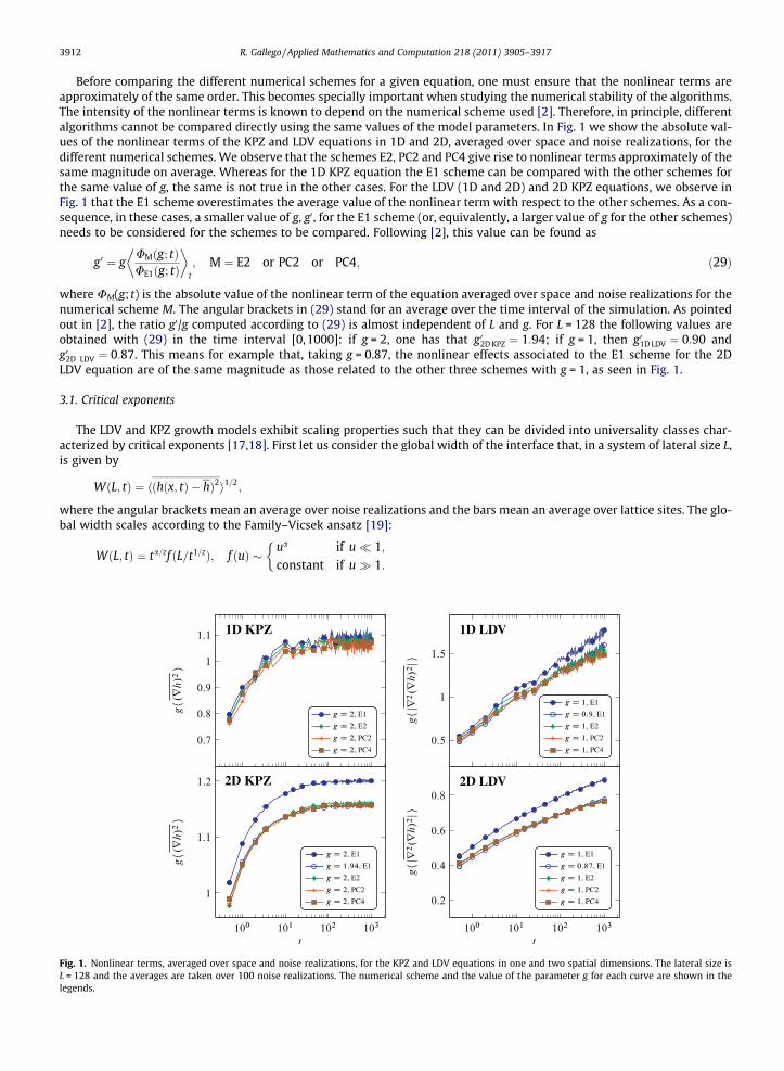
Before comparing the different numerical schemes for a given equation, one must ensure that the nonlinear terms areapproximately of the same order. This becomes specially important when studying the numerical stability of the algorithms.The intensity of the nonlinear terms is known to depend on the numerical scheme used [2]. Therefore, in principle, differentalgorithms cannot be compared directly using the same values of the model parameters. In Fig. 1 we show the absolute val-ues of the nonlinear terms of the KPZ and LDV equations in 1D and 2D, averaged over space and noise realizations, for thedifferent numerical schemes. We observe that the schemes E2, PC2 and PC4 give rise to nonlinear terms approximately of thesame magnitude on average. Whereas for the 1D KPZ equation the E1 scheme can be compared with the other schemes forthe same value of g, the same is not true in the other cases. For the LDV (1D and 2D) and 2D KPZ equations, we observe inFig. 1 that the E1 scheme overestimates the average value of the nonlinear term with respect to the other schemes. As a con-sequence, in these cases, a smaller value of g, g0, for the E1 scheme (or, equivalently, a larger value of g for the other schemes)needs to be considered for the schemes to be compared. Following [2], this value can be found as

Fig. 1.L = 128legends

g0 ¼ gUMðg; tÞUE1ðg; tÞ

t

; M ¼ E2 or PC2 or PC4; ð29Þ

where UM(g; t) is the absolute value of the nonlinear term of the equation averaged over space and noise realizations for thenumerical scheme M. The angular brackets in (29) stand for an average over the time interval of the simulation. As pointedout in [2], the ratio g0/g computed according to (29) is almost independent of L and g. For L = 128 the following values areobtained with (29) in the time interval [0,1000]: if g = 2, one has that g02D KPZ ¼ 1:94; if g = 1, then g01D LDV ¼ 0:90 andg02D LDV ¼ 0:87. This means for example that, taking g = 0.87, the nonlinear effects associated to the E1 scheme for the 2DLDV equation are of the same magnitude as those related to the other three schemes with g = 1, as seen in Fig. 1.

3.1. Critical exponents

The LDV and KPZ growth models exhibit scaling properties such that they can be divided into universality classes char-acterized by critical exponents [17,18]. First let us consider the global width of the interface that, in a system of lateral size L,is given by

WðL; tÞ ¼ hðhðx; tÞ � hÞ2i1=2;

where the angular brackets mean an average over noise realizations and the bars mean an average over lattice sites. The glo-bal width scales according to the Family–Vicsek ansatz [19]:

WðL; tÞ ¼ ta=zf ðL=t1=zÞ; f ðuÞ �ua if u� 1;constant if u� 1:

�

Nonlinear terms, averaged over space and noise realizations, for the KPZ and LDV equations in one and two spatial dimensions. The lateral size isand the averages are taken over 100 noise realizations. The numerical scheme and the value of the parameter g for each curve are shown in the.

R. Gallego / Applied Mathematics and Computation 218 (2011) 3905–3917 3913

Parameter a is the so-called roughness exponent whereas z is the dynamic exponent. Both of them characterize the univer-sality class of the model. The ratio b = a/z is the time exponent. For the LDV model the critical exponents can be calculatedexactly in any dimension d by means of renormalization group techniques [20]: a = (4 � d)/3 and z = (8 � d)/3 (and sob = (4 � d)/(8 + d)). For the 1D KPZ equation the critical exponents a = 1/2 and z = 3/2 (so b = 1/3) can also be calculated ex-actly. Finally, for the 2D KPZ equation, the exponents obtained with field-theoretical methods [21] and a Flory-type approach[22,23] are a = 0.4 and z = 1.6 (so b = 0.25). For small times (t� Lz), a behavior W(L, t) � tb is expected so exponent b can beworked out by measuring the slope of the curve logW(L, t) vs. logt. It is important to emphasize that, in order to compute thetime exponent properly, the value of g must be such that the coupling regime is well displayed. If an unsuitable value of g isused, the computation of the time exponents might not be reliable. At long times (t� Lz) the system reaches a saturationregime where W(L, t) � La. Since the value of z for the LDV equation is larger than that of the KPZ equation, the time it takesthe system to get to saturation for a fixed L is larger for the LDV equation.

The global width for the KPZ and LDV equations in the linear regime are depicted in Fig. 2 for systems of lateral sizesL1D = 2048 and L2D = 512. The values of the nonlinear coupling parameter are gKPZ = 2 and gLDV = 1. The time exponents de-rived from a linear fit of the curves of Fig. 2 are:

Fig. 2.nonlineindicate

b1D KPZ ¼ 0:333� 0:007; b1D LDV ¼ 0:334� 0:006;b2D KPZ ¼ 0:235� 0:006; b2D LDV ¼ 0:217� 0:006:

All the numerical schemes provide approximately the same exponents that are in very good agreement with their theoreticalvalues. For the 2D KPZ equation, a time exponent b � 0.23 is found, a value previously reported in other work using thepseudospectral method E1 [1]. The computed time exponent for the 2D LDV equation is b � 0.22 that is slightly larger thanthe theoretical value of 0.20.

The correlations between fluctuations of the field corresponding to points x and x + r, separated a distance r, are given bythe height-difference correlation functions:

Gmðr; tÞ ¼ hjhðxþ r; tÞ � hðx; tÞjmi1=m; ð30Þ

where m can be in general any real positive number. The average is taken over each site of the system and over the differentrealizations of the noise. Regarding G2(r, t), it has the following behavior:

G2ðr; tÞ ¼ raf ðt=rzÞ; f ðuÞ � ub if u� 1;constant if u� 1:

�

At long times (t� rz), it holds that G2(r, t ?1) � ra and therefore, the roughness exponent a can be computed from the dataof G2 in the saturation regime. The same asymptotic behavior is expected for Gm with m – 2 when multiscaling is not pres-ent. In Section 3.3 the existence of multiscaling is checked numerically by looking at the Gm’s for different values of m.

The exponent a can be obtained alternatively from the structure factor S(q, t) defined by:

Sðq; tÞ ¼ hhðq; tÞhð�q; tÞi:

The structure factor is important in experiments where the power spectrum of the field is measured rather than the fielditself. Numerically S(q, t) is obtained as the square modulus of the Fourier transform of h(x, t). At long times the followingscaling behavior is derived [1]:

Sðq; tÞ � q�d�2a; qzt � 1:

Global width for the KPZ and LDV equations in one and two spatial dimensions. The lateral sizes are L1D = 2048 and L2D = 512. The values of thear coupling parameter are gKPZ = 2 and gLDV = 1. The kind of numerical scheme for each curve is shown in the legends. The straight lines with thed slopes are shown for reference.

3914 R. Gallego / Applied Mathematics and Computation 218 (2011) 3905–3917

In Fig. 3 the correlation function G2(r) at saturation for the KPZ and LDV models integrated with the numerical schemesdescribed in the text is shown. In 2D a spherical average is performed. Again, all the schemes approximately produce thesame results. The values of the roughness exponents obtained from a linear fit of the plots of Fig. 3 are given by:

Fig. 3.describgLDV = 1

a1D KPZ ¼ 0:502� 0:01; a1D LDV ¼ 0:920� 0:08;a2D KPZ ¼ 0:383� 0:02; a2D LDV ¼ 0:690� 0:03:

The values of the exponents are in agreement with their theoretical predictions within error bars.

3.2. Global width at saturation for the 1D KPZ equation

For the 1D KPZ, the behavior of the global width in the steady-state is known exactly [24,25], namely:

WðL; t !1Þ ¼ffiffiffiffiffiffi1

24

rL1=2 � 0:204L1=2:

The previous expression can be used to test the performance of the several numerical schemes. In the computation ofW(L, t ?1) system sizes Li = 2i, with 4 6 i 6 10 were used and the data were averaged over 100 noise realizations. In thecomputation of each value of the width, several tens of points in the bulk of the steady-state region were taken. Then a linearfit of the data (logLi, logW(Li)) was performed, giving parameters A and B such that logW = logA + BlogL. The values of A and Bobtained in this way for the four numerical schemes are:

Parameter

Height-difference correlation functed in the text. The lateral sizes are. Straight lines with slopes corresp

E1

ion G2(r) in the saturation regimeLKPZ = 512, L1D LDV = 256 and L2D

onding to the theoretical predicti

E2

for the KPZ and LDV equations intLDV = 128. The values of the nonlions are shown for reference.

PC2

egrated with the several numericanear coupling parameter g are: gK

PC4

A

0.195 0.195 0.200 0.194 B 0.500 0.501 0.495 0.501

All the schemes give values of A and B are very close to their theoretical values A = 0.204 and B = 0.5. In [1] the authorsshow that a finite-difference based method with a one-step Euler scheme and standard gradient square discretization doesnot give an accurate result as compared with a pseudospectral method (i.e., the E1 method) for the global width in the stea-dy-state. The so-called Lam and Shin discretization [26] for the gradient square (rh)2 gives better results than the standarddiscretization, but they both involve larger fluctuations than a pseudospectral method.

3.3. Multiscaling

In systems exhibiting anomalous scaling the height-difference correlation functions Gm(r, t) are expected to follow thepower-law behavior:

Gmðr; tÞ � rcm ; 1� r � t1=z:

If the cm’s depend on m, the system is said to exhibit multiscaling behavior. Numerically, we can infer the existence multi-scaling by plotting the correlation functions Gm(r, t) for several values of m in the steady state. Multiscaling means that theslopes of the Gm’s depend on m. Both, the KPZ and LDV continuum models are not expected to show multiscaling. In [5] theexistence of multiscaling was suggested for the 1D LDV equation based on the instability of the system against the growth ofisolated pillars of height larger than a certain threshold. However, it was shown in [2] that this conclusion was misleading

l schemesPZ = 2 and

Fig. 4. Height-difference correlation functions Gm(r) (1 6m 6 5) at saturation for the 2D KPZ and 2D LDV equations integrated with the PC4 numericalscheme.

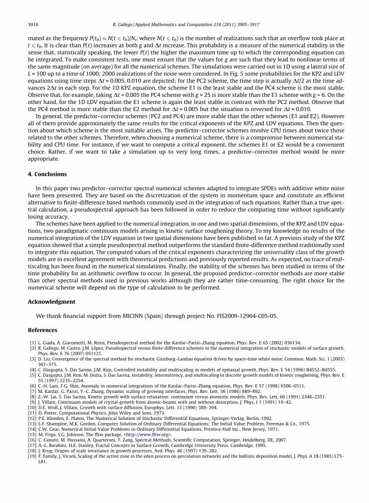
Fig. 5. Temporal evolution of the probabilities for a numerical simulation to undergo an arithmetic overflow for the 1D KPZ and 1D LDV equationsintegrated with the several schemes described in the text. The lateral size is L = 100 and 2000 noise realizations were used. The time step for the PC2 schemeis half the value shown at the top of the figure. The numerical scheme and the value of the parameter g for each curve are shown in the legends.

R. Gallego / Applied Mathematics and Computation 218 (2011) 3905–3917 3915

and an artifact of numerical simulations based on a finite-difference scheme. With a direct computation using a pseudospec-tral method, no multiscaling was observed either in the KPZ equation [1] or in the 1D LDV equation [2].

In Fig. 4 the height-difference correlation functions Gm(r) for 1 6m 6 5 at saturation for the 2D KPZ and 2D LDV equationsintegrated with the PC4 numerical scheme are depicted. As expected, all the correlation functions scale in a similar wayshowing no trace of multiscaling. The same conclusion is reached with the other numerical schemes and also in 1D. Further-more, the temporal evolution of the Gm(r, t)’s for r fixed was considered. In these cases no multiscaling was observed either.

3.4. Numerical stability

The stability of the numerical schemes was tested by measuring the probability for a numerical simulation to undergo anumerical overflow. In a simulation with Nr noise realizations, the probability P(t0) for an overflow to occur at time t0 is esti-

3916 R. Gallego / Applied Mathematics and Computation 218 (2011) 3905–3917

mated as the frequency P(t0) � N(t 6 t0)/Nr, where N(t 6 t0) is the number of realizations such that an overflow took place att 6 t0. It is clear than P(t) increases as both g and Dt increase. This probability is a measure of the numerical stability in thesense that, statistically speaking, the lower P(t) the higher the maximum time up to which the corresponding equation canbe integrated. To make consistent tests, one must ensure that the values for g are such that they lead to nonlinear terms ofthe same magnitude (on average) for all the numerical schemes. The simulations were carried out in 1D using a lateral size ofL = 100 up to a time of 1000; 2000 realizations of the noise were considered. In Fig. 5 some probabilities for the KPZ and LDVequations using time steps Dt = 0.005, 0.010 are depicted; for the PC2 scheme, the time step is actually Dt/2 as the time ad-vances 2Dt in each step. For the 1D KPZ equation, the scheme E1 is the least stable and the PC4 scheme is the most stable.Observe that, for example, taking Dt = 0.005 the PC4 scheme with g = 25 is more stable than the E1 scheme with g = 6. On theother hand, for the 1D LDV equation the E1 scheme is again the least stable in contrast with the PC2 method. Observe thatthe PC4 method is more stable than the E2 method for Dt = 0.005 but the situation is reversed for Dt = 0.010.

In general, the predictor–corrector schemes (PC2 and PC4) are more stable than the other schemes (E1 and E2). Howeverall of them provide approximately the same results for the critical exponents of the KPZ and LDV equations. Then the ques-tion about which scheme is the most suitable arises. The predictor–corrector schemes involve CPU times about twice thoserelated to the other schemes. Therefore, when choosing a numerical scheme, there is a compromise between numerical sta-bility and CPU time. For instance, if we want to compute a critical exponent, the schemes E1 or E2 would be a convenientchoice. Rather, if we want to take a simulation up to very long times, a predictor–corrector method would be moreappropriate.

4. Conclusions

In this paper two predictor–corrector spectral numerical schemes adapted to integrate SPDEs with additive white noisehave been presented. They are based on the discretization of the system in momentum space and constitute an efficientalternative to finite-difference based methods commonly used in the integration of such equations. Rather than a true spec-tral calculation, a pseudospectral approach has been followed in order to reduce the computing time without significantlylosing accuracy.

The schemes have been applied to the numerical integration, in one and two spatial dimensions, of the KPZ and LDV equa-tions, two paradigmatic continuum models arising in kinetic surface roughening theory. To my knowledge no results of thenumerical integration of the LDV equation in two spatial dimensions have been published so far. A previous study of the KPZequation showed that a simple pseudospectral method outperforms the standard finite-difference method traditionally usedto integrate this equation. The computed values of the critical exponents characterizing the universality class of the growthmodels are in excellent agreement with theoretical predictions and previously reported results. As expected, no trace of mul-tiscaling has been found in the numerical simulations. Finally, the stability of the schemes has been studied in terms of thetime probability for an arithmetic overflow to occur. In general, the proposed predictor–corrector methods are more stablethan other spectral methods used in previous works although they are rather time-consuming. The right choice for thenumerical scheme will depend on the type of calculation to be performed.

Acknowledgment

We thank financial support from MICINN (Spain) through project No. FIS2009-12964-C05-05.

References

[1] L. Giada, A. Giacometti, M. Rossi, Pseudospectral method for the Kardar–Parisi–Zhang equation, Phys. Rev. E 65 (2002) 036134.[2] R. Gallego, M. Castro, J.M. López, Pseudospectral versus finite-difference schemes in the numerical integration of stochastic models of surface growth,

Phys. Rev. E 76 (2007) 051121.[3] D. Liu, Convergence of the spectral method for stochastic Ginzburg–Landau equation driven by space-time white noise, Commun. Math. Sci. 1 (2003)

361–375.[4] C. Dasgupta, S. Das Sarma, J.M. Kim, Controlled instability and multiscaling in models of epitaxial growth, Phys. Rev. E 54 (1996) R4552–R4555.[5] C. Dasgupta, J.M. Kim, M. Dutta, S. Das Sarma, Instability, intermittency, and multiscaling in discrete growth models of kinetic roughening, Phys. Rev. E

55 (1997) 2235–2254.[6] C.-H. Lam, F.G. Shin, Anomaly in numerical integrations of the Kardar–Parisi–Zhang equation, Phys. Rev. E 57 (1998) 6506–6511.[7] M. Kardar, G. Parisi, Y.-C. Zhang, Dynamic scaling of growing interfaces, Phys. Rev. Lett. 56 (1986) 889–892.[8] Z.-W. Lai, S. Das Sarma, Kinetic growth with surface relaxation: continuum versus atomistic models, Phys. Rev. Lett. 66 (1991) 2348–2351.[9] J. Villain, Continuum models of crystal-growth from atomic-beams with and without desorption, J. Phys. I 1 (1991) 19–42.

[10] D.E. Wolf, J. Villain, Growth with surface diffusion, Europhys. Lett. 13 (1990) 389–394.[11] D. Potter, Computational Physics, John Wiley and Sons, 1973.[12] P.E. Kloeden, E. Platen, The Numerical Solution of Stochastic Differential Equations, Springer-Verlag, Berlin, 1992.[13] L.F. Shampine, M.K. Gordon, Computer Solution of Ordinary Differential Equations: The Initial Value Problem, Freeman & Co., 1975.[14] C.W. Gear, Numerical Initial Value Problems in Ordinary Differential Equations, Prentice-Hall Inc., New Jersey, 1971.[15] M. Frigo, S.G. Johnson, The fftw package. <http://www.fftw.org>.[16] C. Canuto, M. Hussaini, A. Quarteroni, T. Zang, Spectral Methods, Scientific Computation, Springer, Heidelberg, DE, 2007.[17] A.-L. Barabási, H.E. Stanley, Fractal Concepts in Surface Growth, Cambridge University Press, Cambridge, 1995.[18] J. Krug, Origins of scale invariance in growth processes, Avd. Phys. 46 (1997) 139–282.[19] F. Family, J. Vicsek, Scaling of the active zone in the eden process on percolation networks and the ballistic deposition model, J. Phys. A 18 (1985) L75–

L81.

R. Gallego / Applied Mathematics and Computation 218 (2011) 3905–3917 3917

[20] S. Das Sarma, R. Kotlyar, Dynamical renormalization group analysis of fourth-order conserved growth nonlinearities, Phys. Rev. E 50 (1994) R4275–R4278.

[21] M. Lässig, Quantized scaling of growing surfaces, Phys. Rev. Lett. 80 (1998) 2366–2369.[22] J.M. Kim, J.M. Kosterlitz, Growth in a restricted solid-on-solid model, Phys. Rev. Lett. 62 (1989) 2289–2292.[23] H.G.E. Hentschel, F. Family, Scaling in open dissipative systems, Phys. Rev. Lett. 66 (1991) 1982–1985.[24] J. Krug, P. Meakin, T. Halpin-Healy, Amplitude universality for driven interfaces and directed polymers in random media, Phys. Rev. A 45 (1992) 638–

653.[25] K. Sneppen, J. Krug, M.H. Jensen, C. Jayaprakash, T. Bohr, Dynamic scaling and crossover analysis for the Kuramoto–Sivashinsky equation, Phys. Rev. A

46 (1992) R7351–R7354.[26] C.-H. Lam, F.G. Shin, Improved discretization of the Kardar–Parisi–Zhang equation, Phys. Rev. E 58 (1998) 5592–5595.