Predictive Quantile Regression with Persistent Covariates · PDF filePredictive Quantile...
52
Predictive Quantile Regression with Persistent Covariates Ji Hyung Lee y Department of Economics Yale University (Job Market Paper) November 17, 2012 Abstract This paper develops econometric methods for inference and prediction in quantile regression (QR) allowing for persistent predictors and possible heavy-tailed innovations. Conventional QR econometric techniques lose their validity when predictors are highly persistent as is the case in much of the empirical nance literature where typical predictors include variables such as dividend-price and earnings-price ratios. I adopt and extend a recent methodology called IVX ltering (Magdalinos and Phillips, 2009) that is designed to handle predictor variables with various degrees of persistence. The proposed IVX-QR methods correct the distortion arising from persistent predictors while preserving discriminatory power. The new estimator has a mixed normal limit theory regardless of the degree of persistence in the multivariate predictors. A new computationally attractive testing method for quantile predictability is suggested to simplify implementation for applied work. IVX-QR inherits the robust properties of QR and simulations conrm its substantial superiority over existing methods under thick-tailed errors. The new methods are employed to examine predictability of US stock returns at various quantile levels. The empirical ndings conrm greater forecasting capability at quantiles away from the median and suggest potentially improved forecast models for stock returns. Keywords: Heavy-tailed errors, Instrumentation, IVX ltering, Local to unity, Multivariate predictors, Nonstationary, Predictive regression, Quantile regression, Robustness, Unit root. JEL classication: C22 I am deeply indebted to my advisor Peter Phillips for his endless support and guidance. I am also grateful to Donald Andrews, Timothy Armstrong, Xiaohong Chen, Hiroaki Kaido, Yuichi Kitamura, Taisuke Otsu and Woong Yong Park for valuable suggestions. Comments made by Yoosoon Chang, David Childers, Timothy Christensen, Byoung Gun Park, Zhentao Shi, Minkee Song and Yale econometrics seminar participants are greatly appreciated. All remaining errors are mine. y Email: [email protected]. Tel: 1 203 859 0689. Comments are welcome. 1
Transcript of Predictive Quantile Regression with Persistent Covariates · PDF filePredictive Quantile...

Predictive Quantile Regression with Persistent Covariates�
Ji Hyung Leey
Department of EconomicsYale University
(Job Market Paper)
November 17, 2012
Abstract
This paper develops econometric methods for inference and prediction in quantile regression
(QR) allowing for persistent predictors and possible heavy-tailed innovations. Conventional QR
econometric techniques lose their validity when predictors are highly persistent as is the case
in much of the empirical �nance literature where typical predictors include variables such as
dividend-price and earnings-price ratios. I adopt and extend a recent methodology called IVX
�ltering (Magdalinos and Phillips, 2009) that is designed to handle predictor variables with
various degrees of persistence. The proposed IVX-QR methods correct the distortion arising
from persistent predictors while preserving discriminatory power. The new estimator has a
mixed normal limit theory regardless of the degree of persistence in the multivariate predictors.
A new computationally attractive testing method for quantile predictability is suggested to
simplify implementation for applied work. IVX-QR inherits the robust properties of QR and
simulations con�rm its substantial superiority over existing methods under thick-tailed errors.
The new methods are employed to examine predictability of US stock returns at various quantile
levels. The empirical �ndings con�rm greater forecasting capability at quantiles away from the
median and suggest potentially improved forecast models for stock returns.
Keywords: Heavy-tailed errors, Instrumentation, IVX �ltering, Local to unity, Multivariate
predictors, Nonstationary, Predictive regression, Quantile regression, Robustness, Unit root.
JEL classi�cation: C22
�I am deeply indebted to my advisor Peter Phillips for his endless support and guidance. I am also grateful toDonald Andrews, Timothy Armstrong, Xiaohong Chen, Hiroaki Kaido, Yuichi Kitamura, Taisuke Otsu and WoongYong Park for valuable suggestions. Comments made by Yoosoon Chang, David Childers, Timothy Christensen,Byoung Gun Park, Zhentao Shi, Minkee Song and Yale econometrics seminar participants are greatly appreciated.All remaining errors are mine.
yEmail: [email protected]. Tel: 1 203 859 0689. Comments are welcome.
1

1 Introduction
Predictive regression models are extensively used in empirical macroeconomics and �nance. A
leading example is stock return regression where predictability has been a long standing puzzle.
Forward premium regressions and consumption growth regressions are other commonly occurring
forecast models that similarly present many empirical puzzles. A central econometric issue in all
these models is severe size distortion under the null arising from the presence of persistent pre-
dictors coupled with weak discriminatory power in detecting marginal levels of predictability. The
predictive mean regression literature explored and developed econometric methods for correcting
this distortion and validating inference. A recent review of this research is given in Phillips and
Lee (2012a, Section 2).
Quantile regression (QR) has emerged as a powerful tool for estimating conditional quantiles
since Koenker and Basset (1978). The method has attracted much attention in economics in view of
the importance of the entire response distribution in empirical models. Koenker (2005)�s monograph
provides an excellent overview of the �eld. QR methods are also attractive in predictive regression
because they enable practitioners to focus attention on the quantile structure of �nancial asset
return distribution and provide forecasts at each quantile. This focus permits signi�cance testing
of predictors of individual quantiles of asset returns. Stylized facts of �nancial time series data such
as heavy tails and time varying volatility imply potentially greater predictability at quantiles other
than the median for �nancial data such as asset returns. Standard QR econometric techniques,
however, are not valid when predictors are highly persistent since predictive QR models share the
same econometric issues as their mean regression counterparts.
This paper addresses these issues by developing new methods of inference for predictive QR.
The limit theory I develop for ordinary QR with persistent regressors reveals the source of the
distortion to be greater under (i) stronger endogeneity, (ii) higher levels of persistence and (iii) more
extreme quantiles coupled with stronger tail dependence. To develop QR methods for correcting
the size distortion and conducting valid inference, I adopt a recent methodology called IVX �ltering
developed in Magdalinos and Phillips (2009b). The idea of IVX �ltering is to generate an instrument
of intermediate persistence by �ltering a persistent and possibly endogenous regressor. The new
�ltered IV succeeds in correcting size distortion arising from many di¤erent forms of predictor
persistence while maintaining good discriminatory power in conventional regression settings. I
extend the IVX �lter idea to the QR framework and propose a new approach to inference which
we call IVX-QR.
The proposed IVX-QR estimator has an asymptotically mixed normal distribution in the pres-
ence of multiple persistent predictors. A computationally attractive testing method for quantile
predictability is developed to simplify implementation for applied work. Employing the new meth-
ods, I examine the empirical predictability of monthly stock returns in the S&P 500 index at various
quantile levels. In regressions with commonly used persistent predictors I �nd several quantile spe-
ci�c signi�cant predictors. In particular, over the period of 1927-2005, signi�cant evidence that
dividend-price and dividend-payout ratios have predictive ability for lower quantiles of stock returns
2
is provided by our quantile IVX regressions, while T-bill rate and default yields show predictive
ability over upper quantiles of subsequent returns. The book-to-market value ratio is shown to pre-
dict both lower and upper quantiles of stock returns during the same period. Notably, predictability
appears to be enhanced by using combinations of persistent predictors. IVX-QR corrections ensure
that the quantile predictability results are not spurious even in the presence of multiple persistent
predictors, suggesting the possibility of improved forecast models for stock returns. For example,
the combination of dividend-price ratio and T-bill rate, or the latter with book-to-market ratio are
shown to predict almost all stock return quantiles considered over the 1927-2005 period. The fore-
casting capability of the combination of book-to-market ratio and T-bill rate even remains strong
in the post-1952 data.
Closely related to this paper are recent studies that have investigated inference in QR with
�nancial time series. Xiao (2009) developed limit theory of QR in the presence of unit root regressors
and developed fully-modi�ed methods based on Phillips and Hansen (1990). Cenesizoglu and
Timmermann (2008) introduced the predictive QR framework and found that commonly used
predictor variables a¤ect lower, central and upper quantiles of stock returns di¤erently. Maynard
et al. (2011) examined the issue of persistent regressor in predictive QR by extending the limit
theory of Xiao (2009) to a near-integrated regressor case. The last two papers can be classi�ed into
predictive QR literature since they focused on the prediction of stock return quantiles from lagged
�nancial variables.
The new IVX-QR methods developed in this paper contribute to the predictive QR literature in
several aspects. First, the methods are uniformly valid over the most extensive range of predictor
persistence ever studied, from stationary predictors through to mildly explosive predictors. This
coverage conveniently encompasses existing results for unit root (Xiao, 2009) and near unit root
(Maynard et al., 2011) predictor cases. The uniform validity of the new methods allows for possible
misspeci�cation in predictor persistence. Since the degree of persistence is always imprecisely
determined in practical work, uniformity is a signi�cant empirical advantage. Second, the IVX-QR
methods validate inference under multiple persistent predictors while existing methods control test
size with a single persistent predictor. This feature improves realism in applied work and provides
potentially better forecast models since there are a variety of persistent predictors. Third, the
new method corrects size distortion while preserving substantial local power. This advantage is
critical in �nding marginal levels of predictability in predictive QR with the desired size correction.
IVX-QR also maintains the inherent bene�ts of QR such as markedly superior performance under
thick-tailed errors and the capability of testing predictability at various quantile levels. All these
features make the technique well suited to empirical applications in �nance and macroeconomics.
The paper is organized as follows. Section 2 introduces the model and extends the limit theory
of ordinary QR. Section 3 develops the new IVX-QR methods. Section 4 contains simulation results
and Section 5 illustrates the empirical examples. Section 6 concludes, while lemmas, proofs and
further technical arguments are given in the Appendix.
3

2 Model Framework and Existing Problems
2.1 Model and Assumptions
I �rst discuss the predictive mean regression model and then explain the predictive QR model. The
standard predictive mean regression model is
yt = �0 + �01xt�1 + u0t with E (u0tjFt�1) = 0; (2.1)
where �1 is a K � 1 vector, Ft is a natural �ltration. A vector of predictors xt�1 has the followingautoregressive form
xt = Rnxt�1 + uxt; (2.2)
Rn = IK +C
n�; for some � > 0;
where n is the sample size and C = diag (c1; c2; :::; cK) represents persistence in the multiple
predictors of unknown degree. I allow for more general degrees of persistence in the predictors than
the existing literature. In particular, xt can belong to any of the following persistence categories:
(I0) stationary: � = 0 and j1 + cij < 1, 8i,
(MI) mildly integrated: � 2 (0; 1) and ci 2 (�1; 0), 8i,
(I1) local to unity and unit root: � = 1 and ci 2 (�1;1), 8i,
(ME) mildly explosive: � 2 (0; 1) and ci 2 (0;1), 8i.
For parsimonious characterization of the parameter space the (I1) speci�cation above includes
both conventional integrated (C = 0) and local to unity (C 2 (�1;1) ; C 6= 0) speci�cations. Theinnovation structure allows for linear process dependence for uxt and imposes a martingale di¤erence
sequence (mds) condition for u0t following convention in the predictive regression literature:
u0t � mds (0;�00) ; (2.3)
uxt =
1Xj=0
Fxj"t�j ; "t � mds (0;�) ; � > 0; E k"1k2+� <1; � > 0;
Fx0 = IK ;
1Xj=0
j kFxjk <1; Fx(z) =1Xj=0
Fxjzj and Fx(1) =
1Xj=0
Fxj > 0;
xx =
1Xh=�1
E�uxtu
0xt�h
�= Fx(1)�Fx(1)
0:
Under these conditions, the usual functional limit law holds (Phillips and Solo, 1992):
1pn
bnscXj=1
uj :=1pn
bnscXj=1
"u0j
uxj
#=:
"B0n(s)
Bxn(s)
#=)
"B0(s)
Bx(s)
#= BM
"�00 �0x
�x0 xx
#; (2.4)
4

where B = (B00; B0x)0 is vector Brownian motion (BM). In this instance, the local to unity limit
law for case (I1) also holds (Phillips, 1987):
xbnrcpn=) Jcx(r); where J
cx(r) =
Z r
0e(r�s)CdBx(s) (2.5)
is Ornstein-Uhlenbeck (OU) process.
I now introduce a linear predictive QR model. Given the natural �ltration Ft = �fuj =�u0j ; u
0xj
�0; j � tg, the predictive QR model is
Qyt (� jFt�1) = �0;� + �01;�xt�1. (2.6)
where Qyt (� jFt�1) is a conditional quantile of yt given the information Ft�1
Pr (yt � Qyt (� jFt�1) jFt�1) = � 2 (0; 1) : (2.7)
The model (2.6) may be considered a generalization of the predictive regression model (2.1), as it
analyzes other quantile predictability as well as the central quantile of yt. Under the assumption
of symmetrically distributed errors, (2.6) with � = 0:5 reduces to (2.1) since Qyt (0:5jFt�1) =E (ytjFt�1). Letting the QR innovation u0t� := yt�Qyt (� jFt�1) = yt��0;� ��01;�xt�1, one obtains
yt = �0;� + �01;�xt�1 + u0t� (2.8)
= �0�Xt�1 + u0t� ;
where Xt�1 = (1; x0t�1)0, and
Qu0t� (� jFt�1) = 0 (2.9)
from (2.7). In fact, (2.9) is the only moment condition so innovation with in�nite mean or variance
is allowed1. The robustness of QR to thick-tailed errors enables better econometric inference than
mean regression for �nancial applications using heavy-tailed data. To see the relation of (2.1) and
(2.8), recenter the innovation of (2.1) as u0t� = u0t � F�1u0 (�), then (2.9) follows, and
yt = �0;� + �01xt�1 + u0t� and �0;� = �0 + F
�1u0 (�) ;
which is the construction of Xiao (2009).
By de�ning a piecewise derivative of the loss function in the QR � (u) = � � 1 (u < 0) (seebelow), it is easy to show the QR �induced� innovation � (u0t� ) � mds (0; � (1� �)), and the
1The functional CLT in (2.4) holds under the �nite second moment condition as in (2.3), and we will need �-stable limit laws for in�nite mean/variance innovation cases. To stay focused, I only consider limit theory with �nitevariance innovations here but IVX-QR limit theory can be extended to the case of in�nite mean/variance innovations,as we will show in later work. The self-normalized IVX-QR estimator shows extremely good normal approximationsunder in�nite mean/variance errors in the simulation section.
5

following functional law holds
1pn
bnrcXt=1
" � (u0t� )
uxt
#=)
"B � (r)
Bx(r)
#= BM
"� (1� �) � �x
�x � xx
#: (2.10)
This functional law drives the main asymptotics below.
Some regularity assumptions on the conditional density of u0t� are imposed.
Assumption 2.1 (i) The sequence of stationary conditional pdf ffu0t� ;t�1 (�)g evaluated at zerosatis�es a FCLT with a non-degenerate mean fu0� (0) = E [fu0t� ;t�1 (0)] > 0;
1pn
bnrcXt=1
(fu0t� ;t�1 (0)� fu0� (0)) =) Bfu0� (r) :
(ii) For each t and � 2 (0; 1), fu0t� ;t�1 is bounded above with probability one around zero, i.e.,
jfu0t� ;t�1 (�)j <1 w.p.1
where � can be arbitrarily close to zero.
Remark 2.1 Assumption 2.1-(i) is not restrictive considering that an mds structure is commonlyimposed on u0t (hence u0t� ) in the predictive regression literature. Assumption 2.1-(ii) is a standard
technical condition used in the QR literature, enabling expansion of not everywhere di¤erentiable
objective functions after smoothing with the conditional pdf fu0t� ;t�1.
2.2 Limit Theory Extension of Nonstationary Quantile Regression
This subsection extends the existing limit theory of ordinary QR. This extension is of some inde-
pendent interest and is useful in revealing the source of the problems that arise from persistent
regressors in QR. The ordinary QR estimator has the form:
�QR
� = argmin�
nXt=1
���yt � �0Xt�1
�(2.11)
where �� (u) = u (� � 1 (u < 0)), � 2 (0; 1) is the asymmetric QR loss function. The notation
Xt�1 = (1; x0t�1)0 includes the intercept and the regressor xt�1 whose speci�cation is given in (2.2).
I employ di¤erent normalizing matrices according to the regressor persistence:
Dn :=
8>>>><>>>>:
pnIK+1 for (I0),
diag(pn; n
1+�2 IK) for (MI),
diag(pn; nIK) for (I1),
diag(pn; n�Rnn) for (ME).
(2.12)
6

Using the Convexity Lemma (Pollard, 1990), as in Xiao (2009), I prove the next theorem that
encompasses the limit theory for the unit root case (Theorem 1 in Xiao; 2009), stationary local to
unity case (Proposition 2 in Maynard et al; 2011) and stationary case (Koenker, 2005). This paper
adds to the QR literature by extending that limit theory to the (MI) and (ME) cases.
Theorem 2.1
Dn
��QR
� � ���=)
8>>>>>>>>>>>>>>><>>>>>>>>>>>>>>>:
N
0; �(1��)
fu0� (0)2
"1 0
0 �1xx
#!for (I0),
N
0; �(1��)
fu0� (0)2
"1 0
0 V �1xx
#!for (MI),
fu0� (0)�1"
1RJcx(r)
0RJcx(r)
RJcx(r)J
cx(r)
0
#�1 "B � (1)RJcx(r)dB �
#for (I1),
MN
240; �(1��)fu0� (0)
2
24 1 0
0�~Vxx
��13535 for (ME),
where Vxx =R10 erCxxe
rCdr; ~Vxx =R10 e�rCYCY
0Ce
�rCdr and YC � N�0;R10 e�rCxxe�rCdr
�:
2.3 Sources of Nonstandard Distortion and Correction Methods
Theorem 2.1 shows that the limit distribution in the (I1) case is nonstandard and nonpivotal.
To see the source of nonstandard distortion clearly, I further analyze the limit distribution of
the slope coe¢ cient estimator. For simplicity, assume K = 1 and uxt � mds (0;�xx), then it is
straightforward to show that
n�b�QR1;� � �1;�� � fu0� (0)
�1R�JcxdB �R ��Jcx�2 ;
where �Jcx = Jcx(r) �R 10 J
cx(r)dr is the demeaned OU process. Using the orthogonal decomposition
of Brownian motion (Phillips, 1989) dB � = dB � :x +�� �x�xx
�dBx we have
n�b�QR1;� � �1;�� � fu0� (0)
�1"R
�JcxdB � :xR ��Jcx�2 +
�� �x
�xx
� R �JcxdBxR ��Jcx�2#:
Note that: R�JcxdB � :xR ��Jcx�2 �MN
0;� � :x
�Z ��Jcx�2��1!
;
7

with � � :x = �(1� �)���1xx�2 �x and � �x = E [1 (u0t� < 0)uxt] = E�1�u0t < F�1u0 (�)
�uxt�. Now
assume a researcher uses the ordinary QR standard error:
s:e(b�QR1;� ) =24�(1� �)fu0� (0)
2
1
n2
nXt=1
�x�t�1
�2!�1351=2 ;then with the standardized notation
��Icx;Wx
�= �
�1=2xx
��Jcx; Bx
�, the t-ratio becomes:
tb�1;� =
�b�QR1;� ��1;��s:e(b�QR1;� )
��1�
�2 �x�xx�(1��)
�1=2N(0; 1) +
��2 �x
�xx�(1��)
�1=2 R�IcxdWxhR(�Icx)
2i1=2
�h1� � (�)2
i1=2Z| {z } +� (�) �LUR(c)| {z }
standard inference nonstandard distortion
(2.13)
where Z and �LUR(c) stand for a standard normal distribution and the local unit root t-statistics,
respectively, and
� (�) = corr (1 (u0t� < 0) ; uxt) 6= corr(u0t; uxt) = �:
Remark 2.2 As the analytical expression (2.13) shows, the nonstandard distortion becomes greaterwith (i) smaller jcj and (ii) larger j� (�)j. Condition (i) is well known from mean predictive re-
gression literature where the distortion from the highly left-skewed feature of �LUR(c) with small jcjhas been studied. Condition (ii) is a special feature of nonstationary quantile regression, see Xiao
(2009) for strict unit root regressors. Note that:
� (�) =
�E [1 (u0t� < 0)uxt]
�xx�(1� �)
�1=2=
E�1�u0t < F�1u0 (�)
�uxt�
�xx�(1� �)
!1=2;
so the explicit source of distortion from persistence and nonlinear dependence is provided by this
analysis. The commonly used lower tail dependence measure is
�L = lim�!0+
P�u0t < F�1u0 (�)juxt < F�1ux (�)
�= lim
�!0+
E�1�u0t < F�1u0 (�)
�1�uxt < F�1ux (�)
���(1� �) :
Thus, � (�) is a measure of the dependence between the linear dependence (E [u0tuxt]) and tail
dependence (E�1�u0t < F�1u0 (�)
�1�uxt < F�1ux (�)
��). If we consider a lower quantile prediction,
such as � = 0:05 or 0:1, the distortion is more a¤ected by tail dependence than by correlation. This
is consistent with the recent �ndings that a precise VaR estimation depends on the tail dependence
structure (e.g., Embrechts et al.,1997). The distortion stemming from the interaction between
persistence and tail dependence has not been properly addressed in the literature.
8

To correct the nonstandard distortion in (2.13), we may consider two solutions. The �rst is
to construct a con�dence interval (CI) for c, such as Stock�s CI (1991), and correct the distortion
through an induced CI for �1;� . This is the main idea of the Bonferroni methods, which are fre-
quently used in predictive mean regression (e.g., Cavanagh et al.,1995; Campbell and Yogo, 2006).
In predictive QR, Maynard et al. (2011) employed the same idea. For a single local to unity (I1)
predictor, these methods successfully correct the distortion, but lose their validity when predictor
persistence belongs to (MI) or (I0) spaces (Phillips, 2012)2. In addition, Bonferroni methods are
not applicable in the presence of multivariate nonstationary predictors (multiple ci�s). The second
solution to correct for nonstandard distortion, which this paper follows, is to use IVX �ltering tech-
nique (Magdalinos and Phillips, 2009). Methods based on the IVX �ltering technique are discussed
in the next section. The main advantages of these methods over (currently available) Bonferroni
methods are its uniform validity over a much wider range of predictor persistence including (I0)
through (ME) and applicability to multiple persistent predictors, as well as a single persistent
predictor.
3 IVX-QR Methods
It is convenient to transform the model (2.8) to remove the explicit intercept term:
yt� = �01;�xt�1 + u0t� (3.1)
where yt� := yt��QR
0;� (�) = yt��0;�+Op�n�1=2
�is the zero-intercept QR dependent variable. This
is analogous to the demeaning process in the predictive mean regression in preparation for tests of
the slope coe¢ cient. Using the pre-estimatedpn-consistent estimation �
QR
0;� (�) is asymptotically
innocuous (see Appendix 7.2). After estimating �IV XQR
1;� , we may compute �IV XQR
0;� for inference
on �0;� as well (see Appendix 7.3).
3.1 IVX Filtering
This subsection reviews a new �ltering method, IVX �ltering (Magdalinos and Phillips, 2009). The
idea can be explained by comparing it to commonly used �ltering methods. For simplicity, �rst
assume xt belongs to (I1). Filtering persistent data xt to generate ~zt can be described as
~zt = F ~zt�1 +4xt
with a �ltering coe¢ cient F and �rst di¤erence operator 4.When F = 0K then ~zt = 4xt and we simply take the �rst di¤erence to remove the persistence
in xt. First di¤erencing is the most common technique employed by applied researchers, and it
leads to the (I0) limit theory in Theorem 2.1. Thus, the standard normal (or chi square) inference is
2The Bonferroni methods based on a uniformly valid CI for c, rather than Stock�s CI, may provide validity over(MI) or (I0) spaces. These extensions, however, have not been developed in the predictive regression literature yet.
9

achieved. The drawback to �rst di¤erencing is the substantial loss of statistical power in detecting
predictability of xt�1 on yt. Taking the �rst di¤erence of a regression equation makes both xt�1and yt much noisier and �nding the relationship between two noisy processes is a statistically
challenging task. In terms of convergence rate, the �rst di¤erence reduces the n-rate (for the (I1)
case) to thepn-rate (for the (I0) case), thereby seriously diminishing local power. At the cost of
this substantial loss, the �rst di¤erence technique corrects the nonstandard distortion in (2.13).
When F = IK then ~zt = xt so we may use level data without any �ltering. The statistical
power is preserved in this way, since it is easy to detect if a persistent xt�1 has a nonnegligible
explanatory power on noisy yt. This is clear from the n-rate of convergence of (I1) limit theory
(maximum rate e¢ ciency) in Theorem 2.1. However, inference still su¤ers from the serious size
distortion in (2.13).
The main idea of IVX �ltering is to �lter xt to generate ~zt with (MI) persistence - intermediate
between �rst di¤erencing and the use of levels data. In particular, we choose F = Rnz as follows:
~zt = Rnz~zt�1 +4xt, Rnz = IK +Czn�, (3.2)
where � 2 (0; 1) , Cz = czIK , cz < 0 and ~z0 = 0
The parameters � 2 (0; 1) and cz < 0 are speci�ed by the researcher. As is clear from the con-
struction, Rnz is between 0K and IK but closer to IK especially for large n: This construction
is designed to preserve local power as far as possible while achieving the desirable size correction.
The ~zt essentially belongs to an (MI) process so the limit theory of the (MI) case in Theorem 2.1
is obtained by using ~zt as instruments. The IVX �ltering exploits advantages both from using level
(power) and the �rst di¤erence (size correction) of persistent data. It leads to the intermediate
signal strength n1+�2 . At the cost of the slight reduction in convergence rate compared to the level
data, the �ltering achieves the desired size correction. Simulation in Section 4 shows that this cost
is not substantial so we have comparable, and sometimes better local power to n-consistent testing
such as Q-test of Campbell and Yogo (2006). To summarize
Table 1: Comparisons of level, �rst di¤erenced and IVX-�ltered data
level �rst di¤erence IVX �ltering
Discriminatory power Yes No Yes
Size correction No Yes Yes
Rate of convergence npn n
1+�2
Assume now that xt falls into one of three speci�cations: (I0), (MI) and (I1). When xt belongs
to (I1), the IVX �ltering reduces the persistence to (MI) as described above. If xt belongs to (MI)
or (I0), the �ltering maintains the original persistence. This is how we achieve the uniform validity
over the range of (I0)-(I1). This automatic adjustment applies to several persistent predictors
10

simultaneously, thereby accommodating multivariate persistent regressors. When xt belongs to
(ME), the IVX estimation becomes equivalent to OLS for the mean regression case (Phillips and
Lee, 2012b). The same principle works for QR, delivering uniformly valid inference in QR over
(I0)-(ME) predictors (Proposition 3.1 and 3.2 below).
3.2 IVX-QR Estimation and Limit Theory
I propose new IVX-QR methods that are based on the use of IVX �ltered instruments. Since the
rate of convergence of IVX-QR will di¤er according to predictor persistence, I unify notation for
the data with the following embedded normalizations:
~Zt�1;n := ~D�1n ~zt�1 and Xt�1;n := ~D�1
n xt�1: (3.3)
where
~Dn =
8><>:pnIK for (I0),
n1+(�^�)
2 IK for (MI) and (I1),
n(�^�)Rnn for (ME),
and � ^ � = min (�; �). I also de�ne the di¤erent asymptotic moment matrices for the (MI) and
(I1) cases in a uni�ed way:
Vcxz :=
(V xzz =
R10 erCzxxe
rCzdr; when � 2 (0; � ^ 1) ;Vxx =
R10 erCxxe
rCdr; when � 2 (0; �) :(3.4)
and
cxz :=
8><>:�C�1z
�xx +
RdJcxJ
c0x
; if � = 1;
�C�1z fxx + CVxxg ; if � 2 (�; 1) ;Vcxz = Vxx if � 2 (0; �) :
(3.5)
Considering the conditional moment restriction Qu0t� (� jFt�1) = 0, or
E�� � 1
�yt� � �1;�
0xt�1�jFt�1
�= 0;
a natural procedure of estimating �1;� using IVX �ltering is to minimize the L2-distance of the sum
of the empirical moment conditions that use IVX ~zt�1 from information set Ft�1.
De�nition 3.1 (IVX-QR estimation) The IVX-QR estimator �1;� for �1;� is de�ned as
�IV XQR
1;� = arg inf�1
1
2
nXt=1
mt (�1)
!0Wn
nXt=1
mt (�1)
!; (3.6)
where Wn is an arbitrary weighting matrix and
mt (�1) = ~zt�1�� � 1
�yt� � �1
0xt�1��= ~zt�1 � (u0t� (�1)) :
11

The minimization (3.6) leads to the following approximate FOC:
nXt=1
~Zt�1;n
�� � 1
�yt� �
��IV XQR
1;�
�0xt�1
��= op(1): (3.7)
The asymptotic theory of �IV XQR
1;� follows from this condition. The next theorem gives the limit
theory of the IVX-QR estimator under various degrees of predictor persistence.
Theorem 3.1 (IVX-QR limit theory)
~Dn
��IV XQR
1;� � �1;��=)
8>>>><>>>>:N�0; �(1��)
fu0� (0)2
�1xx
�for (I0),
MN�0; �(1��)
fu0� (0)2
�1cxzVcxz
��1cxz
�0� for (MI) and (I1),
MN
�0; �(1��)
fu0� (0)2
�~Vxx
��1�for (ME).
Unlike Theorem 2.1, the limit theory is (mixed) normal for all cases, and the limit variances
are easily estimated. The self-normalized estimator given in the following theorem provides a
convenient tool for uni�ed inference across the (I0), (MI), (I1) and (ME) cases.
Proposition 3.1 (Self-normalized IVX-QR) For (I0), (MI), (I1) and (ME) predictors,
\fu0� (0)2
�(1� �)
��IV XQR
1;� � �1;��0 �
X 0P ~ZX� ��IV XQR
1;� � �1;��=) �2 (K) ,
where X 0P eZX = X 0 ~Z�~Z 0 ~Z��1
~Z 0X =�Pn
t=2 xt�1~z0t�1� �Pn
t=2 ~zt�1~z0t�1��1 �Pn
t=2 xt�1~z0t�1�0 and
\fu0� (0) is any consistent estimator for fu0� (0) 3.
Using Proposition 3.1, we can test the linear hypothesis H0 : �1;� = �01;� for any given �01;� .
More generally, consider a set of r linear hypotheses
H0 : H�1;� = h�
with a known r�K matrix H and a known vector h� . In this case the null test statistics are formed
as follows with the corresponding chi-square limit theory
\fu0� (0)2
�(1� �)
�H�
IV XQR
1;� � h��0 n
H�X 0P ~ZX
��1H 0o�1 �
H�IV XQR
1;� � h��=) �2 (r) :
3.3 IVX-QR Inference: Testing Quantile Predictability
Theorem 3.1 and Proposition 3.1 allow for testing of a general linear hypothesis with multiple
persistent predictors. When the number of parameter K is large, the procedure (3.6) may be3The kernel density estimation with standard normal kernel functions and a bandwidth choice of Silvermann�s
rule is used in the simulation and empirical results below.
12

computationally demanding since the optimization of a nonconvex objective requires grid search
with several local optima. Considering that the usual hypothesis of interest in predictive regression
is the null of H0 : �1;� = 0 (signi�cant testing), I propose an alternative testing procedure that is
computationally attractive. Recall the DGP we impose is
yt� = �01;�xt�1 + u0t� .
Based on the fact that xt�1 and ~zt�1 are "close" to each other, we use ordinary QR on ~zt�1 to test
H0 : �1;� = 0. Speci�cally, consider the simple QR regression procedure
IV XQR1;� = argmin
nXt=1
���yt� � 01~zt�1
�:
We then have the following asymptotics of null test statistics:
Theorem 3.2 Under H0 : �1;� = 0;
~Dn
� IV XQR1;� � �1;�
�=)
8>>>><>>>>:N�0; �(1��)
fu0� (0)2
�1xx
�for (I0),
N�0; �(1��)
fu0� (0)2V
�1cxz
�for (MI) and (I1),
MN
�0; �(1��)
fu0� (0)2
�~Vxx
��1�for (ME).
:
The above limit theory also holds under local alternatives of the form H0 : �1;� =b1;�n� with some
� > 0. We achieve asymptotic normality of the null test statistics simply by replacing the regressor
xt�1 with ~zt�1. The �nal pivotal test statistics can be obtained by a similar self-normalization as
given in the next theorem.
Proposition 3.2 Under H0 : �1;� = 0;
\fu0� (0)2
�(1� �)
� IV XQR1;� � �1;�
�0 �~Z 0 ~Z��
IV XQR1;� � �1;��=) �2 (K) :
for (I0), (MI), (I1) and (ME) predictors.
Since QR algorithms are available in standard statistical software, Proposition 3.2 provides a
uniform inference tool that involves easy computation. If we want to test the predictability of a
speci�c subgroup among our predictors, say H0 : �11;� = �12;� = 0, then we could use the following
test statistics
\fu0� (0)2
�(1� �)
�H IV XQR1;�
�0�H�~Z 0 ~Z��1
H 0��1 �
H IV XQR1;�
�=) �2 (2)
where H =
"1 0 01�(K�2)
0 1 01�(K�2)
#:
13

4 Simulation
In this section, I conduct simulations to observe the size and power performance of IVX-QR in-
ference methods. Theorems 3.1 and 3.2 show that a larger IVX persistence (�) leads to a more
e¢ cient test, while a smaller � generally achieves better size corrections. Using simulations with
settings similar to those used in the existing predictive regression literature, I provide guidance for
the choice of � in applied work.
The following DGP is imposed:
yt = �0;� + �01;�xt�1 + u0t;� ; (4.1)
xt = �x +Rxt�1 + uxt.
where �x = 0; R = IK +Cn and
ut =
"u0t
uxt
#� iid Fu
�0(K+1)�1;�(K+1)�(K+1)
�: (4.2)
The IVX is constructed as (3.2) and the inference uses Proposition 3.2. I normalize Cz = �5IKand vary � to show performance according to varying IVX persistence.
4.1 Size and Power Performance with a Single Persistent Predictor
This subsection shows simulations with a single local to unity (K = 1; � = 1) regressor. Although
IVX-QR methods allow testing for predictability at various quantile levels, I focus on the central
(median) quantile to compare its performance to that of existing mean predictability tests. In
particular, the IVX median test is compared to the methods of Campbell and Yogo (2006; CY-Q)
and Kostakis et al (2012; IVX-mean).
For the distribution Fu in (4.2), I �rst use a normal distribution with the variance
� =
1 �
� 1
!;
with � = �0:95. This value re�ects the realistic error correlation in predictive regressions, such asdividend-price ratio. It also has been frequently used in the literature, such as in Campbell and
Yogo (2006) and Jansson and Moreira (2006).
Tables 2 and 3 summarize the size performances of the IVX-QR and CY-Q tests. The empirical
size is calculated from the rejection frequency of a one-sided test of H0 : �1;� = 0 versus H1 :
�1;� > 0 with � = 0:5. For simplicity, I set �0;� = 0. Note that the CY-Q test uses the null of
H 00 : Et�1 [yt] = �1 = 0 instead of H0 de�ned above. The assumptions of conditional mean/median
zero yt under H0 and H 00 are then exploited to compare these two di¤erent types of tests. The
introduction of estimated intercepts to relax this assumption is discussed in Appendix 7.5. The
14
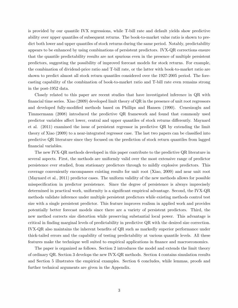
nominal size is 0:05 with 2,500 repetitions (S).
Table 2: Finite sample sizes of IVX-QR and CY-Q tests (n = 100)
R = 1 R = 0:98 R = 0:9 R = 0:8 R = 0:5 R = 0
S = 2500 c = 0 c = �2 c = �10 c = �20 c = �50 c = �100� = IVXQR IVXQR IVXQR IVX-QR IVXQR IVXQR
0.95 0.0724 0.0624 0.0564 0.0456 0.0492 0.0376
0.85 0.0552 0.0584 0.0468 0.0472 0.0412 0.0392
0.75 0.062 0.0572 0.0396 0.0456 0.048 0.0304
0.65 0.0608 0.0556 0.0428 0.0504 0.0324 0.0412
0.55 0.0444 0.0424 0.0456 0.0484 0.0544 0.0344
CY-Q 0.05 0.046 0.0608 0.0792 N/A N/A
It is evident from Table 2 that the size of IVX-QR is uniformly well controlled in the case of a
pure stationary predictor (R = 0) to a unit root predictor (R = 1), supporting one of the main
contributions of this paper. The CY-Q test also shows good size properties for (near) unit root
predictors (R 2 [0:9; 1]), but the performance decays for less persistent predictors. This is becauseStock�s (1991) CI for R is invalid for (near) stationary regressors, thereby a¤ecting the Bonferroni
CI for �14. I also con�rm the robustness of IVX-QR for various values of � 2 [0:55; 0:95]. A similar
result holds with n = 200.
Table 3: Finite sample sizes of IVX-QR and CY-Q tests (n = 200)
R = 1 R = 0:99 R = 0:95 R = 0:9 R = 0:5 R = 0
S = 2500 c = 0 c = �2 c = �10 c = �20 c = �100 c = �200� = IVXQR IVXQR IVXQR IVXQR IVXQR IVXQR
0.95 0.0664 0.0616 0.052 0.0492 0.0556 0.042
0.85 0.0716 0.0604 0.0548 0.0564 0.0444 0.0376
0.75 0.0552 0.0652 0.044 0.0504 0.0416 0.0388
0.65 0.0492 0.0492 0.0492 0.0432 0.0544 0.0416
0.55 0.0472 0.0472 0.0448 0.0484 0.0412 0.0388
CY-Q 0.0492 0.0508 0.05 0.05 N/A N/A
To investigate power performances, I generate a sequence of local alternatives with H�1n : �1n =bn
in (4.1) for integer values b � 0 (� = 0:5 is suppressed) and observe the performances of the IVX-QR, IVX-mean, and CY-Q tests. For the distribution Fu, I employ normal and t-distributions with
four to one (Cauchy) degrees of freedom. As expected, two mean predictability tests dominate
IVX-QR under normally distributed errors. For the �nite sample performance of the IVX-mean
and CY-Q tests under normally distributed innovations, see Kostakis et al. (2012). I report the
power performances with t(4)-t(1) innovations to highlight possible improvements when using IVX-
4For a detailed explanation of this problem, the reader is referred to recent work by Phillips (2012).
15

QR in cases of thick-tailed errors. It is widely known that �nancial asset returns have heavy-tailed
distributions (e.g., Cont, 2001). The cz = �5; � = 0:95 speci�cation is employed because it
e¤ectively controls the size. With sample size n = 200, I observe the cases of c 2 f0;�2;�20;�40gre�ecting persistent predictors in practice.
Figures 1-4 illustrate the results. For unit root (� = 1) and near unit root (� = 0:99) predictors,
the test performance rankings with t(3)-t(4) errors are mixed. IVX-QR performs best with mildly
persistent predictors, as shown by � = 0:9 and 0:8 in the simulation. For in�nite variance (t(2))
and mean (t(1)) errors, IVX-QR shows the best performance across all scenarios.
Considering that much applied work also uses the intercept term in the regression, IVX-QR
with dequantiling, as in (3.1), is compared with the IVX-mean and CY-Q tests. Appendix 7.5
shows the results with the same ranking patterns as above.
In summary, IVX-QR testing with a single persistent predictor is competitive when we have
heavy-tailed errors and when the persistence of predictors is close to near stationary (mildly inte-
grated). Because we can obtain information on the tail properties of any given data and partial
information, albeit imperfect, on the persistence of predictors, one may decide which test is better
to use. All three tests perform well in terms of size and power except for the CY-Q test in cases
of mildly integrated predictors. Therefore, several valid methods can test the predictive ability of
a single persistent predictor on given �nancial asset returns. Note that, unlike the CY-Q test, the
IVX-mean and IVX-QR tests can employ multiple persistent predictors. In addition, the IVX-QR
test can analyze the predictability of other quantiles in addition to the median, providing greater
applicability for prediction tests. Size properties of IVX-QR prediction tests on various quantiles
are analyzed in the next subsection.
16

Figure 1: Power curves of IVX-QR, IVX-mean and CY-Q tests
c = 0 (n = 200; R = 1) with t(4), t(3), t(2) and t(1) innovations.
0 0.01 0.02 0.03 0.04 0.050
0.2
0.4
0.6
0.8
1t(4)
IVXQRIVXmeanCYQNominal Size
0 0.01 0.02 0.03 0.04 0.050
0.2
0.4
0.6
0.8
1t(3)
IVXQRIVXmeanCYQNominal Size
0 0.01 0.02 0.03 0.04 0.050
0.2
0.4
0.6
0.8
1t(2)
IVXQRIVXmeanCYQNominal Size
0 0.01 0.02 0.03 0.04 0.050
0.2
0.4
0.6
0.8
1t(1)
IVXQRIVXmeanCYQNominal Size
Figure 2: Power curves of IVX-QR, IVX-mean and CY-Q tests
c = �2 (n = 200; R = 0:99) with t(4), t(3), t(2) and t(1) innovations.
0 0.01 0.02 0.03 0.04 0.050
0.2
0.4
0.6
0.8
1t(4)
IVXQRIVXmeanCYQNominal Size
0 0.01 0.02 0.03 0.04 0.050
0.2
0.4
0.6
0.8
1t(3)
IVXQRIVXmeanCYQNominal Size
0 0.01 0.02 0.03 0.04 0.050
0.2
0.4
0.6
0.8
1t(2)
IVXQRIVXmeanCYQNominal Size
0 0.01 0.02 0.03 0.04 0.050
0.2
0.4
0.6
0.8
1t(1)
IVXQRIVXmeanCYQNominal Size
17

Figure 3: Power curves of IVX-QR, IVX-mean and CY-Q tests
c = �20 (n = 200, R = 0:9) with t(4), t(3), t(2) and t(1) innovations.
0 0.02 0.04 0.06 0.08 0.10
0.2
0.4
0.6
0.8
1t(4)
IVXQRIVXmeanCYQNominal Size
0 0.02 0.04 0.06 0.08 0.10
0.2
0.4
0.6
0.8
1t(3)
IVXQRIVXmeanCYQNominal Size
0 0.02 0.04 0.06 0.08 0.10
0.2
0.4
0.6
0.8
1t(2)
IVXQRIVXmeanCYQNominal Size
0 0.02 0.04 0.06 0.08 0.10
0.2
0.4
0.6
0.8
1t(1)
IVXQRIVXmeanCYQNominal Size
Figure 4: Power curves of IVX-QR, IVX-mean and CY-Q tests
c = �40 (n = 200; R = 0:8) with t(4), t(3), t(2) and t(1) innovations.
0 0.05 0.1 0.15 0.20
0.2
0.4
0.6
0.8
1t(4)
IVXQRIVXmeanCYQNominal Size
0 0.05 0.1 0.15 0.20
0.2
0.4
0.6
0.8
1t(3)
IVXQRIVXmeanCYQNominal Size
0 0.05 0.1 0.15 0.20
0.2
0.4
0.6
0.8
1t(2)
IVXQRIVXmeanCYQNominal Size
0 0.05 0.1 0.15 0.20
0.2
0.4
0.6
0.8
1t(1)
IVXQRIVXmeanCYQNominal Size
18

4.2 Size Properties of Prediction Tests on Various Quantiles
Despite the vast literature on predictive mean regression, few studies have considered predicting
other quantile levels of �nancial returns, such as the tail or shoulder (for exceptions, see Maynard
et al., 2011; Cenesizoglu and Timmermann, 2008). This paper develops the �rst valid method to
test various quantile predictability of asset returns in the presence of multiple persistent predictors.
In this subsection, I focus on large sample performance (n = 700) to guarantee accurate density
estimation at the tails, e.g., the 5% quantile. Imprecise density estimation at extreme quantiles
with �nite sample is a common problem in QR. Large sample sizes are not uncommon in �nancial
applications, and the empirical work in the next section corresponds to one of those applications.
The simulation environment used to test the size properties of various quantile predictions is
similar to the earlier subsection, but I now include the estimated intercept to mimic the common
practical work. Dequantiling in (3.1) is therefore used for all IVX-QR simulations in this subsection.
The persistence parameter ci is selected from f0;�2;�5;�7;�70g. This set represents a set ofpersistent predictors including R = 0:9 (MI) through R = 1 (unit root). Normal and t-distributions
are used for Fu and the number of replications is 1000. All null test statistics use the same
hypothesis: H0 : �1;� = 0 with a nominal size of 0.05. I use a cut-o¤ rule of 8% for the reasonable
size results because 7-8% is the permissible empirical size level corresponding to a nominal 5% size
(see Campbell and Yogo, 2006). The results of these simulations are presented in Tables 4-8 below;
the size performances exceeding 8% are shown in bold.
I �rst investigate the size properties of ordinary QR methods. Table 4 below summarizes the size
properties of ordinary QR t-statistics in (2.13) with a single persistent predictor when � = �0:95.The nonstandard distortion increases with more persistent predictors (smaller c). As Remark
2.2 suggests, the tail dependence structure of Fu signi�cantly a¤ects the magnitude of the size
distortion. For a t-distribution with stronger tail dependence (smaller degrees of freedom), more
severe size distortion arises at the tail than at the median, while the tendency does not impact
normally distributed errors (tail independent). The overall results indicate the invalidity of the
ordinary QR technique in the presence of persistent predictors.
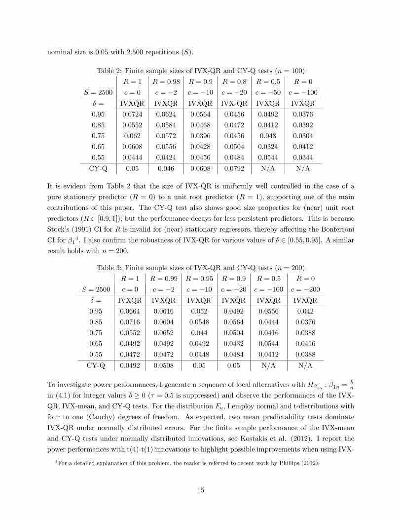
The size performances of the IVX-QR methods with Cz = �5 and � = 0:5 are reported in
Table 5. Under normally distributed errors, the size corrections are remarkable, con�rming the
uniform validity of IVX-QR methods at various quantiles. For heavy-tailed errors with stronger
tail dependence, the results still hold in all but a few tail cases. Table 6 shows the results with
� = 0:6. In this case, we lose a few more unit root (c = 0) cases under stronger tail dependence.
Extensive simulation results indicate that the IVX-QR correction methods control sizes remarkably
well across all quantiles when � is less than 0.7. When � exceeds 0.7, the test tends to over-reject
at tails while maintaining good performances at inner quantiles5.
5Simulation results with various choices of � are readily available upon request.
19

Table 4: Size Performances(%) of Ordinary QR (n = 700, S = 1000)
Normally distributed errors
� = 0.05 0.1 0.2 0.3 0.4 0.5 0.6 0.7 0.8 0.9 0.95
c = 0 14.5 13.5 15.0 15.5 16.3 17.8 17.0 16.3 16.0 13.1 14.5c = �2 10.6 9.9 11.0 12.5 12.9 11.9 11.9 11.4 9.8 9.6 11.5c = �5 8.7 8.1 8.3 8.4 7.7 9.4 8.9 9.8 7.5 11.0 10.6c = �7 9.7 9.2 7.4 6.3 7.4 6.2 6.2 7.1 7.4 7.8 9.5c = �70 6.7 6.1 6.0 4.2 5.2 3.8 4.2 4.6 4.6 5.6 8.2
t(4) errors
� = 0.05 0.1 0.2 0.3 0.4 0.5 0.6 0.7 0.8 0.9 0.95
c = 0 17.2 16.6 16.7 13.9 13.1 13.2 14.6 14.1 16.7 18.0 18.3c = �2 13.0 13.4 11.0 9.9 9.8 9.7 8.1 10.5 13.8 12.8 16.3c = �5 12.0 10.0 10.3 6.0 7.5 6.4 6.5 8.5 9.8 11.6 11.2c = �7 10.5 10.4 8.3 6.8 5.7 6.7 5.6 8.1 8.1 10.8 10.1c = �70 10.0 6.7 6.9 4.8 4.1 4.6 4.7 4.3 6.1 6.0 10.1
t(3) errors
� = 0.05 0.1 0.2 0.3 0.4 0.5 0.6 0.7 0.8 0.9 0.95
c = 0 18.1 17.0 13.5 12.5 12.3 11.5 11.9 12.9 14.4 17.1 17.6c = �2 14.4 13.3 11.1 8.5 8.5 9.1 9.2 11.2 11.3 13.3 15.0c = �5 11.8 11.5 8.1 9.1 6.6 8.1 7.4 6.5 8.4 11.4 12.9c = �7 12.5 8.1 10.1 7.5 5.5 7.1 5.8 6.9 6.4 9.4 13.5c = �70 10.0 8.9 5.4 4.8 5.5 3.6 4.2 4.7 6.5 7.8 9.3
t(2) errors
� = 0.05 0.1 0.2 0.3 0.4 0.5 0.6 0.7 0.8 0.9 0.95
c = 0 20.3 16.1 11.3 11.1 9.1 8.5 8.5 10.4 12.3 14.2 16.2c = �2 15.8 12.4 10.7 8.3 8.6 5.8 6.7 8.1 11.8 12.0 15.7c = �5 13.0 9.0 6.7 6.2 5.4 5.4 4.7 6.5 8.4 12.9 13.7c = �7 12.2 10.7 7.8 5.6 4.1 3.9 5.8 5.3 7.9 10.7 13.9c = �70 7.2 7.1 6.8 4.5 4.6 3.4 3.7 5.3 7.0 8.3 8.6
20

Table 5: Size Performances(%) of IVX-QR with � = 0:5 (n = 700, S = 1000)
Normally distributed errors
� = 0.05 0.1 0.2 0.3 0.4 0.5 0.6 0.7 0.8 0.9 0.95
c = 0 7.0 6.0 6.9 4.6 5.1 4.5 6.7 6.0 6.5 5.9 8.0
c = �2 7.4 5.6 4.6 4.3 4.8 3.7 5.3 4.0 4.8 5.8 7.5
c = �5 6.6 5.5 5.1 4.2 4.8 3.2 3.7 4.5 4.7 5.2 6.8
c = �7 5.5 5.6 4.5 4.9 3.6 3.4 3.7 4.1 5.1 4.4 7.3
c = �70 4.9 4.8 4.6 4.0 3.1 3.4 3.7 4.1 3.9 4.8 7.1
c = �700 6.5 6.8 4.3 6.2 4.3 4.6 5.4 4.8 4.0 4.2 6.5
t(4) errors
� = 0.05 0.1 0.2 0.3 0.4 0.5 0.6 0.7 0.8 0.9 0.95
c = 0 9.1 7.5 6.0 5.9 6.4 4.5 6.0 6.1 6.5 8.8 9.5c = �2 7.4 5.6 4.0 3.7 3.4 3.8 5.5 5.0 4.9 6.0 9.8c = �5 7.5 7.2 5.2 5.0 3.5 3.3 3.4 3.4 5.2 6.0 7.5
c = �7 6.5 7.6 5.6 4.9 3.3 3.8 4.8 4.6 5.8 4.8 6.8
c = �70 6.5 5.6 5.2 4.1 3.5 3.9 3.2 3.8 5.4 5.6 7.1
c = �700 8.0 7.6 4.8 5.4 4.9 3.9 3.9 3.8 6.6 5.7 7.8
t(3) errors
� = 0.05 0.1 0.2 0.3 0.4 0.5 0.6 0.7 0.8 0.9 0.95
c = 0 9.8 10.2 7.8 6.4 5.2 5.1 4.8 4.8 6.7 7.6 11.1c = �2 7.7 8.3 6.2 4.5 4.4 3.1 4.4 5.5 4.8 7.2 8.6c = �5 6.5 7.0 6.0 4.6 3.7 4.1 3.5 3.0 5.2 6.0 6.5
c = �7 6.0 5.7 4.9 3.4 3.3 3.7 3.6 4.9 5.2 5.5 7.3
c = �70 7.2 7.3 6.1 4.1 4.0 2.8 4.4 5.5 5.0 6.1 5.2
c = �700 6.7 6.9 5.8 4.8 4.0 4.4 4.9 4.5 6.0 5.0 6.5
t(2) errors
� = 0.05 0.1 0.2 0.3 0.4 0.5 0.6 0.7 0.8 0.9 0.95
c = 0 10.5 8.9 6.3 5.8 4.7 4.6 5.3 6.4 8.0 5.9 7.7
c = �2 7.9 5.9 6.1 3.3 4.5 3.9 3.2 4.1 7.2 6.5 5.6
c = �5 5.3 5.9 6.0 6.0 3.7 3.3 5.3 4.2 7.1 6.5 6.2
c = �7 6.8 6.4 6.4 3.8 3.3 4.1 4.3 3.7 6.0 8.4 7.3
c = �70 4.9 7.9 6.6 4.6 3.9 4.3 4.1 4.8 6.3 5.9 5.2
c = �700 4.4 5.5 6.2 6.4 4.7 3.8 5.6 5.3 5.2 6.8 3.8
21
Table 6: Size Performances(%) of IVX-QR with � = 0:6 (n = 700, S = 1000)
Normally distributed errors
� = 0.05 0.1 0.2 0.3 0.4 0.5 0.6 0.7 0.8 0.9 0.95
c = 0 7.0 7.8 8.9 6.7 6.7 6.8 8.5 7.9 8.2 7.2 8.9c = �2 7.6 6.0 5.1 5.0 4.6 4.1 5.1 4.1 5.3 5.7 7.2
c = �5 6.6 6.1 4.7 4.3 4.6 3.0 4.7 4.5 5.0 5.4 6.4
c = �7 7.1 5.9 4.9 5.3 4.1 4.0 4.1 4.4 4.7 4.9 6.5
c = �70 5.1 5.5 4.3 3.3 3.3 3.1 3.5 4.8 4.4 5.0 7.7
c = �700 7.4 6.8 4.7 5.7 4.4 4.6 5.5 4.7 3.7 4.1 7.0
t(4) errors
� = 0.05 0.1 0.2 0.3 0.4 0.5 0.6 0.7 0.8 0.9 0.95
c = 0 10.8 8.4 8.2 7.7 7.6 5.6 6.8 8.0 9.7 9.1 9.7c = �2 8.0 6.7 5.8 4.4 4.4 4.8 5.4 6.2 6.3 6.5 10.3c = �5 8.4 7.9 5.4 4.5 3.9 3.3 4.4 3.7 4.7 6.2 7.7
c = �7 7.5 8.1 5.5 5.0 2.5 4.0 4.8 4.8 6.2 5.5 7.4
c = �70 6.9 6.4 5.0 4.2 3.7 4.5 3.2 4.1 5.6 6.0 6.9
c = �700 8.0 7.2 4.9 5.6 4.7 4.1 3.7 4.1 6.7 6.0 7.7
t(3) errors
� = 0.05 0.1 0.2 0.3 0.4 0.5 0.6 0.7 0.8 0.9 0.95
c = 0 10.6 11.4 9.4 7.1 7.1 7.2 5.6 7.7 7.7 9.1 10.7c = �2 9.1 7.6 6.0 5.8 4.8 3.9 4.9 5.4 5.7 7.8 8.2c = �5 5.8 7.4 5.6 5.1 4.1 3.8 3.5 3.7 5.6 6.9 7.2
c = �7 8.2 6.5 5.1 4.2 4.3 4.2 3.5 4.3 5.7 5.0 7.8
c = �70 7.6 7.4 5.8 3.2 4.0 3.1 4.6 4.6 5.2 5.8 6.7
c = �700 7.0 6.8 5.5 3.9 3.9 4.3 5.3 4.4 6.5 5.3 6.5
t(2) errors
� = 0.05 0.1 0.2 0.3 0.4 0.5 0.6 0.7 0.8 0.9 0.95
c = 0 13.5 9.7 7.3 6.6 5.6 5.2 6.5 7.6 9.7 7.4 8.8c = �2 8.1 6.6 6.6 4.4 4.3 3.9 3.1 4.7 8.6 7.9 5.5
c = �5 6.5 7.3 6.4 5.3 4.9 3.8 5.4 4.7 7.1 7.6 7.1
c = �7 8.0 7.7 6.2 4.6 3.3 3.8 4.4 4.3 6.7 8.2 7.5
c = �70 5.1 7.2 6.1 4.5 4.1 3.5 3.9 4.8 6.8 6.0 6.5
c = �700 3.8 5.1 5.6 6.2 4.8 3.9 6.5 5.4 5.7 6.8 4.1
22

I now consider the predictive QR scenario with multiple persistent predictors (K = 2). This
scenario has rarely been explored but is highly relevant in empirical practice (e.g., dividend-price
ratio and Treasury bill rate). The bivariate predictor persistence (c1; c2) is again selected from
f0;�2;�5;�7;�70g and all other simulation settings are the same as before. For the innovationstructure, I borrow a calibration technique to avoid lengthy documentation. In the next section,
speci�cation with two predictors of book-to-market ratio and Treasury bill rate is shown to predict
stock returns at various quantile levels from January 1952 to December 2005. To support the
empirical �nding, the estimated correlation of the predictive QR application is used:
� =
0B@ 1 �0:78 �0:17�0:78 1 0:21
�0:17 0:21 1
1CA :
Table 7 shows the size properties of ordinary QR test statistics. The size distortion is larger
when there is more than one persistent predictor, which corroborates the bene�ts of the IVX-QR
method�s validating inference under multiple manifestations of predictor persistence. Table 8 shows
acceptable size results of the IVX-QR tests at various quantile levels. The size correction under
normally distributed errors works very well for most quantiles. Performances at tails are good
except for a few cases, and results at inner quantiles from 0.1 to 0.9 are satisfactory. Under strong
tail dependent innovations (t(4) or t(3) errors), the IVX-QR corrections for multiple persistent
predictors at � = 0:05 or 0:1 are partly acceptable. The IVX-QR correction result for these
extreme cases suggests a need for new methods to handle extremal quantiles. One promising
potential solution could be the use of a recent development in extremal QR limit theory (e.g.,
Chernozhukov, 2005; Chernozhukov and Fernandez-Val, 2012), but I leave this for future research.
In summary, IVX-QR methods demonstrate reliable size performances for all relevant speci�ca-
tions with single and multiple persistent predictors, except for a few extreme cases. The practical
bene�ts of IVX-QR inference will be illustrated through empirical examples in the next section.
23
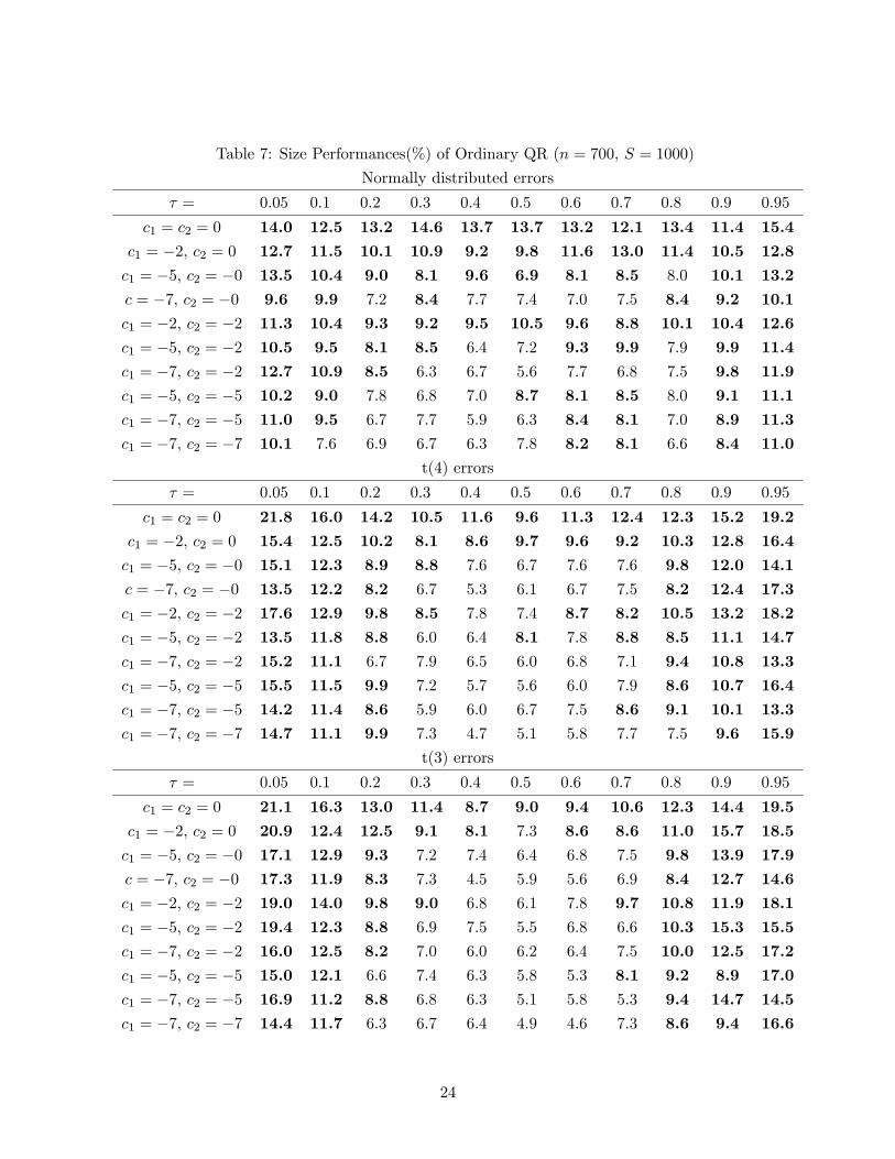
Table 7: Size Performances(%) of Ordinary QR (n = 700, S = 1000)
Normally distributed errors
� = 0.05 0.1 0.2 0.3 0.4 0.5 0.6 0.7 0.8 0.9 0.95
c1 = c2 = 0 14.0 12.5 13.2 14.6 13.7 13.7 13.2 12.1 13.4 11.4 15.4c1 = �2, c2 = 0 12.7 11.5 10.1 10.9 9.2 9.8 11.6 13.0 11.4 10.5 12.8c1 = �5, c2 = �0 13.5 10.4 9.0 8.1 9.6 6.9 8.1 8.5 8.0 10.1 13.2c = �7, c2 = �0 9.6 9.9 7.2 8.4 7.7 7.4 7.0 7.5 8.4 9.2 10.1c1 = �2, c2 = �2 11.3 10.4 9.3 9.2 9.5 10.5 9.6 8.8 10.1 10.4 12.6c1 = �5, c2 = �2 10.5 9.5 8.1 8.5 6.4 7.2 9.3 9.9 7.9 9.9 11.4c1 = �7, c2 = �2 12.7 10.9 8.5 6.3 6.7 5.6 7.7 6.8 7.5 9.8 11.9c1 = �5, c2 = �5 10.2 9.0 7.8 6.8 7.0 8.7 8.1 8.5 8.0 9.1 11.1c1 = �7, c2 = �5 11.0 9.5 6.7 7.7 5.9 6.3 8.4 8.1 7.0 8.9 11.3c1 = �7, c2 = �7 10.1 7.6 6.9 6.7 6.3 7.8 8.2 8.1 6.6 8.4 11.0
t(4) errors
� = 0.05 0.1 0.2 0.3 0.4 0.5 0.6 0.7 0.8 0.9 0.95
c1 = c2 = 0 21.8 16.0 14.2 10.5 11.6 9.6 11.3 12.4 12.3 15.2 19.2c1 = �2, c2 = 0 15.4 12.5 10.2 8.1 8.6 9.7 9.6 9.2 10.3 12.8 16.4c1 = �5, c2 = �0 15.1 12.3 8.9 8.8 7.6 6.7 7.6 7.6 9.8 12.0 14.1c = �7, c2 = �0 13.5 12.2 8.2 6.7 5.3 6.1 6.7 7.5 8.2 12.4 17.3c1 = �2, c2 = �2 17.6 12.9 9.8 8.5 7.8 7.4 8.7 8.2 10.5 13.2 18.2c1 = �5, c2 = �2 13.5 11.8 8.8 6.0 6.4 8.1 7.8 8.8 8.5 11.1 14.7c1 = �7, c2 = �2 15.2 11.1 6.7 7.9 6.5 6.0 6.8 7.1 9.4 10.8 13.3c1 = �5, c2 = �5 15.5 11.5 9.9 7.2 5.7 5.6 6.0 7.9 8.6 10.7 16.4c1 = �7, c2 = �5 14.2 11.4 8.6 5.9 6.0 6.7 7.5 8.6 9.1 10.1 13.3c1 = �7, c2 = �7 14.7 11.1 9.9 7.3 4.7 5.1 5.8 7.7 7.5 9.6 15.9
t(3) errors
� = 0.05 0.1 0.2 0.3 0.4 0.5 0.6 0.7 0.8 0.9 0.95
c1 = c2 = 0 21.1 16.3 13.0 11.4 8.7 9.0 9.4 10.6 12.3 14.4 19.5c1 = �2, c2 = 0 20.9 12.4 12.5 9.1 8.1 7.3 8.6 8.6 11.0 15.7 18.5c1 = �5, c2 = �0 17.1 12.9 9.3 7.2 7.4 6.4 6.8 7.5 9.8 13.9 17.9c = �7, c2 = �0 17.3 11.9 8.3 7.3 4.5 5.9 5.6 6.9 8.4 12.7 14.6c1 = �2, c2 = �2 19.0 14.0 9.8 9.0 6.8 6.1 7.8 9.7 10.8 11.9 18.1c1 = �5, c2 = �2 19.4 12.3 8.8 6.9 7.5 5.5 6.8 6.6 10.3 15.3 15.5c1 = �7, c2 = �2 16.0 12.5 8.2 7.0 6.0 6.2 6.4 7.5 10.0 12.5 17.2c1 = �5, c2 = �5 15.0 12.1 6.6 7.4 6.3 5.8 5.3 8.1 9.2 8.9 17.0c1 = �7, c2 = �5 16.9 11.2 8.8 6.8 6.3 5.1 5.8 5.3 9.4 14.7 14.5c1 = �7, c2 = �7 14.4 11.7 6.3 6.7 6.4 4.9 4.6 7.3 8.6 9.4 16.6
24

Table 8: Size Performances(%) of IVX-QR with � = 0:5 (n = 700, S = 1000)
Normally distributed errors
� = 0.05 0.1 0.2 0.3 0.4 0.5 0.6 0.7 0.8 0.9 0.95
c1 = c2 = 0 10.8 8.4 8.0 7.8 6.4 6.5 7.0 6.3 8.0 6.1 10.4c1 = �2, c2 = 0 10.3 7.9 6.6 3.9 5.2 5.0 5.6 5.4 5.6 6.8 7.6
c1 = �5, c2 = �0 9.9 8.3 6.5 4.8 4.5 5.2 5.4 4.2 5.3 6.6 10.4c = �7, c2 = �0 9.8 4.7 5.0 4.9 5.3 5.0 5.2 5.3 4.7 6.6 7.6
c1 = �2, c2 = �2 8.0 5.8 5.5 4.7 5.3 5.4 4.9 4.1 7.8 4.3 8.5c1 = �5, c2 = �2 8.6 6.3 5.0 3.3 4.4 3.9 3.9 3.5 3.9 6.6 6.8
c1 = �7, c2 = �2 8.7 6.9 6.0 3.9 3.5 3.9 4.4 5.0 4.1 4.7 7.5
c1 = �5, c2 = �5 7.3 5.3 4.6 4.8 4.4 5.3 4.6 3.8 7.1 5.6 8.4c1 = �7, c2 = �5 7.7 6.1 4.5 3.2 4.6 4.0 3.7 3.3 4.5 6.8 5.9
c1 = �7, c2 = �7 6.7 5.7 4.7 4.9 4.0 4.6 4.2 3.9 6.3 4.9 8.0
t(4) errors
� = 0.05 0.1 0.2 0.3 0.4 0.5 0.6 0.7 0.8 0.9 0.95
c1 = c2 = 0 16.5 13.0 8.0 6.9 6.0 5.2 6.7 8.0 6.4 11.6 13.9c1 = �2, c2 = 0 11.9 9.0 7.5 5.9 4.8 5.1 4.6 5.6 6.7 8.8 13.1c1 = �5, c2 = �0 12.3 8.0 6.9 4.9 5.3 3.5 5.3 5.1 6.3 9.0 11.2c = �7, c2 = �0 10.9 11.4 7.5 5.7 4.6 4.6 5.0 5.1 5.6 8.3 11.8c1 = �2, c2 = �2 13.7 10.1 6.6 4.1 3.8 3.8 4.3 5.2 5.4 7.9 11.5c1 = �5, c2 = �2 10.3 8.0 6.4 4.1 4.0 4.0 4.6 4.7 5.1 8.0 9.6c1 = �7, c2 = �2 10.7 7.9 5.9 3.5 3.0 3.0 3.8 5.4 5.7 7.7 10.7c1 = �5, c2 = �5 11.7 8.9 5.5 3.9 4.0 4.0 4.3 4.8 5.0 7.4 9.5c1 = �7, c2 = �5 9.5 7.5 5.9 4.1 3.8 3.0 3.9 4.7 4.8 8.0 9.5c1 = �7, c2 = �7 10.8 8.5 5.6 3.1 3.7 3.7 4.3 4.5 5.0 6.3 9.2
t(3) errors
� = 0.05 0.1 0.2 0.3 0.4 0.5 0.6 0.7 0.8 0.9 0.95
c1 = c2 = 0 15.0 12.4 7.9 7.4 6.2 7.4 6.3 7.6 7.1 10.5 14.1c1 = �2, c2 = 0 15.4 9.6 8.8 4.3 6.3 4.4 4.3 7.0 7.3 12.3 13c1 = �5, c2 = �0 11.0 11.7 6.6 6.5 4.1 4.5 4.1 6.7 7.2 9.1 14.1c = �7, c2 = �0 10.9 10.7 6.6 5.1 3.6 3.7 4.9 4.7 6.7 9.7 9.7c1 = �2, c2 = �2 11.5 9.3 5.7 4.5 4.1 4.8 4.2 5.2 5.4 9.0 9.2c1 = �5, c2 = �2 12.7 8.8 6.4 3.4 5.1 3.3 3.7 5.9 5.9 9.8 10.5c1 = �7, c2 = �2 11.7 10.6 5.4 6.2 3.6 3.9 4.0 6.5 7.0 7.4 11.8c1 = �5, c2 = �5 11.4 7.7 4.9 4.2 3.6 4.3 3.7 4.3 5.2 7.9 8.5c1 = �7, c2 = �5 10.6 8.0 6.8 4.0 5.2 3.6 3.3 5.7 6.0 10.5 9.5c1 = �7, c2 = �7 11.4 6.5 4.8 4.1 3.2 3.5 3.4 4.0 5.5 7.4 7.5
25

5 Quantile Predictability of Stock Returns
It is often standard practice in �nance literature to test stock return predictability using various
economic and �nancial state variables as predictors. There is considerable disagreement in the
empirical literature as to the predictability of stock returns when using a predictive mean regression
framework (e.g., Campbell and Thompson, 2007; Goyal and Welch, 2007). In this section, I brie�y
discuss the empirical rationale for predictive QR, which makes this approach attractive for stock
return regressions. I then use the IVX-QR procedure to examine stock return predictability at
various quantile levels with commonly used persistent predictors.
5.1 Empirical Motivation: Why Predictive QR?
To understand the empirical motivation for predictive QR, I begin with some selected stylized facts
on �nancial assets. Cont (2001) notes that �nancial asset returns often have (i) conditional heavy
tails, (ii) time-varying volatility, and (iii) asymmetric distributions. In stock return prediction tests,
these stylized facts may motivate the use of QR, as now discussed.
To illustrate I consider a simple model for an asset return yt:
yt = �t�1 + �t�1"t with "t � iid F"; (5.1)
so that �t�1 and �t�1 signify the location (mean) and scale (volatility) conditional on Ft�1. Ifwe assume E ("tjFt�1) = 0, then E (ytjFt�1) = �t�1 and the predictive mean regression model
uses �t�1 = �0 + �1xt�1 with predictor xt�1. Inconclusive empirical results from mean regressions
suggest that the magnitude of �1 is small with most predictors xt�1. Now also assume a stochastic
volatility model: �t�1 = �0 + �1xt�1. If a predictor xt�1 signi�cantly in�uences the volatility of
stock returns yt, as many economic factors do, then �1 6= 0. In fact, the conditional variance
often shows a greater systematic (or cyclical) variation than the conditional mean of stock returns,
suggesting that j�1j > j�1j. The predictive QR now reduces to
Qyt (� jFt�1) = �0 + �1xt�1 + (�0 + �1xt�1)Q"t (�) = �0;� + �1;�xt�1
where
�0;� = �0 + �0Q"t (�) and �1;� = �1 + �1Q"t (�) :
When "t is close to symmetric, �1;� ' �1 with � = 0:5. When �1 is small, such as for a near-
martingale stock return, �1;� ' �1Q"t (�) and the absolute value of �1;� increases as � ! 0 (or
� ! 1). This tendency may explain why the location (mean/median) of stock returns is more
di¢ cult to predict than other statistical measures, such as the scale (dispersion). Even when �1 is
not negligible, the magnitude of �1Q"t (�) would help in �nding the predictability. Note also that
when "t � iid t (�) in (5.1), the absolute value of �1;� with � 6= 0:5 increases as � decreases. Thelocation of stock return predictability varies depending on the magnitude and sign of (�1, �1), but
QR can e¤ectively locate it. Therefore, QR provides forecasts on stock return quantiles where the
26

actual predictability is more likely to exist. This illustrates the rationale for using QR to predict
stock returns with thick tails (smaller �) and cyclical movements in conditional volatility (non-zero
�1).
Lastly, consider an asymmetrically distributed "t in (5.1) with jQ"t (�)j > jQ"t (1� �)j for a� < 0:5. In this case, predictor variables with nonneglible (�1, �1) may predict lower quantiles of
stock returns better than upper quantiles. These asymmetric predictable patterns and quantile-
speci�c predictors can be detected through predictive QR.
Although the above example is stylized, we clearly see the advantages of QR in a stock return
regression framework. Many of the results hypothesized above are con�rmed in the empirical results
below.
5.2 Empirical Results: IVX-QR Testing
I now show empirical results of stock return prediction tests using IVX-QR. Excess stock returns
are measured by the di¤erence between the S&P 500 index including dividends and the one month
treasury bill rate. I focus on eight persistent predictors: dividend price (d/p), earnings price (e/p),
book to market (b/m) ratios, net equity expansion (ntis), dividend payout ratio (d/e), T-bill rate
(tbl), default yield spread (dfy), term spread (tms) and various combinations of the above variables.
The full sample period is January 1927 to December 2005. These data sets are standard and
have been extensively used in the predictive regression literature. Cenesizoglu and Timmermann
(2008) and Maynard et al., (2011) recently used the same data set in a QR framework6. Following
Cenesizoglu and Timmermann (2008), I classify the predictors into three categories.
� Valuation ratios
� dividend-price ratio (d/p)
� earnings-price ratio (e/p)
� book-to-market ratio (b/m)
� Bond yield measures
� three-month T-bill rate (tbl)
� term spread (tms)
� default yield (dfy)
� Corporate �nance variables
� dividend-payout ratio (d/e)
6 I would like to thank Yini Wang for providing the data set. For detailed constructions and economic foundationsof the data set, see Goyal and Welch (2007). Note that Maynard et al. (2011) and Cenesizoglu and Timmermann(2008) also considered stationary predictors other than the eight persistent predictors I use.
27

� net equity expansion (ntis)
I employ the IVX-QR methods to illustrate the bene�ts of these new methods. In particular,
I �rst investigate the quantile predictability of stock returns using individual predictors and then
analyze the improved predictive ability of various combinations of predictors. This application both
complements and supplements the mean predictive regressions. There will be more applications of
quantile-speci�c predictors that are useful for asset pricing and portfolio decisions-making.
The null test statistics in Proposition 3.2 is used with IVX �ltering parameters � = 0:5 and
Cz = �5IK because the speci�cation showed uniformly good size properties for both single and
multiple persistent predictors in the earlier section. Table 5 below reports the univariate regression
results, where p-values (%) are rounded to one decimal place for exposition. The results shown in
bold imply the rejection of the null hypothesis of no predictability at 5% level.
Table 5: p-values(%) of quantile prediction tests (1927:01-2005:12)
Univariate regressions with each of the eight predictors: d/p, d/e, b/m, tbl, dfy, ntis, e/p, tms
� = 0.05 0.1 0.2 0.3 0.4 0.5 0.6 0.7 0.8 0.9 0.95
d/p 1.0* 0.1* 0.3* 14.1 76.0 50.3 17.6 0.5* 6.4 9.6 1.8*
d/e 0.0* 0.0* 0.0* 0.4* 1.8* 16.4 59.5 49.8 89.7 5.8 0.3*
b/m 0.2* 0.0* 0.1* 0.4* 22.5 83.3 56.0 2.8* 6.2 0.8* 1.7*
tbl 46.0 50.3 10.6 11.7 3.6* 12.3 6.0 19.9 3.9* 0.6* 0.3*
dfy 33.6 66.3 98.5 89.8 53.5 5.6 3.0* 0.1* 0.0* 0.0* 0.1*
e/p 75.3 89.8 42.1 51.4 96.5 71.2 89.7 47.2 55.7 33.0 32.6
ntis 23.0 96.7 24.1 13.2 10.1 73.8 71.6 74.1 65.9 94.8 32.5
tms 41.8 15.6 82.5 68.2 26.6 36.7 14.6 58.1 23.2 13.0 16.3
The result is roughly consistent with the results of Maynard et al. (2011) and Cenesizoglu and
Timmermann (2008). I �nd signi�cant upper quantile predictive ability for the tbl and dfy, and
lower quantile predictive power for the d/e. Evidence of both lower and upper quantile predictability
from b/m is also similar. One notable di¤erence is the evidence of predictability at lower quantiles
with d/p. Overall, I �nd little evidence of predictability at the median. The results con�rm many
hypothesized empirical results in the earlier section - the weak predictability at the mean/median
of stock returns, the stronger forecasting capability at quantiles away from the median and several
quantile speci�c (lower, upper or both quantiles) predictors .
For multivariate regression applications, I use selective predictor combinations for illustrative
purposes. The selection scheme is as follows: First, I choose signi�cant predictors from univariate
regression results (d/p, d/e, b/m, tbl, and dfy in this instance). Second, I classify the chosen
predictors into three groups - group L, group B and group U. Group L corresponds to the group
with signi�cant lower-quantile predictors, and so on for the other groups. I select one predictor
from each group to produce a bivariate predictor.
28

� Group of lower quantile predictors (Group L): d/p and d/e
� Both upper and lower quantile predictor (Group B): b/m
� Group of upper quantile predictors (Group U): tbl and dfy
Finally, I choose predictor combinations exhibiting little evidence of comovement between the
predictors. Although evidence of comovement between predictors does not completely reduce the
appeal of the combinations; we may prefer less-comoving systems for better forecast models7.
I employ two diagnostic tests to observe evidence of comovement between persistent predictors:
(i) the correlation of xt�1, and (ii) the cointegration tests between xt�1. The two measures will
provide evidence of comovement between all (I0)-(ME) predictors (see Appendix 7.6). I �nd little
evidence of comovement between (d/p, tbl), (d/e, dfy), (d/e, b/m), (tbl, bm) and (dfy, b/m).
The above selection scheme is used primarily for illustrative purposes, and I do not rule out the
possibility of signi�cant results from other combinations8. However, it is partly justi�able from a
theoretical perspective. For example, both d/p and b/m are ratios measuring undervaluation in the
stock market and are thus positively correlated to subsequent returns, while tbl is a macro variable
that may have di¤erent predictive patterns. If we choose between (d/p, b/m) and (tbl, b/m), the
above economic rational recommends (tbl, b/m) because it shares fewer common characteristics.
Diagnostic tests indicate strong comoving evidence between d/p and b/m but not between tbl
and b/m, corresponding with the economic foundation. Similar arguments hold for the group of
corporate �nance variables measuring managerial �nancing activity. Managers�timing of issuing
equity precedes falling stock prices, indicating negative correlation with stock returns.
From Table 6 below, I con�rm that many predictors are jointly signi�cant at various quantiles
with much stronger evidences than univariate regressions. Many existing studies only considered
a single persistent predictor when they considered the spurious predictability from the size distor-
tion. The results below illustrate the possibility of better forecast models with multiple persistent
predictors that are not subject to spurious forecasts. We can proceed with more than two predictor
models in a similar way.
7Phillips (1995) provided robust inference methods in cointegrating mean regression models with possibly comovingpersistent regressors (FM-VAR regressions). Introducing the robust feature into the current framework (allowingnonsingular xx in (2.10)) will be left for future research.
8Results for other combinations are readily available upon request.
29

Table 6: p-values(%) of quantile prediction tests (1927:01-2005:12)
Multivariate regressions with two predictors among d/p, d/e, tbl, dfy and b/m
� = 0.05 0.1 0.2 0.3 0.4 0.5 0.6 0.7 0.8 0.9 0.95
d/p, tbl 0.4* 0.1* 0.8* 2.4* 1.0* 7.6 8.6 0.0* 1.2* 1.0* 0.0*
d/e, tbl 0.0* 0.0* 0.0* 0.2* 0.1* 0.7* 6.8 36.6 6.0 0.0* 0.0*
d/e, dfy 13.4 3.6* 13.0 20.2 33.0 11.0 2.6* 0.2* 0.0* 0.5* 0.2*
d/e, b/m 0.0* 0.0* 0.0* 0.1* 1.2* 57.2 40.6 16.3 2.1* 0.0* 0.0*
tbl, b/m 0.6* 0.0* 0.2* 2.7* 6.0 4.6* 0.6* 0.6* 0.1* 0.2* 2.9*
dfy, b/m 0.9* 0.2* 0.9* 9.4 12.5 14.6 19.1 0.1* 0.1* 0.0* 0.3*
I run the same analysis for post-1952 data. Many papers have reported that the stock return
predictability becomes much weaker from January 1952 to December 2005 (see Campbell and Yogo,
2006; Kostakis et al. 2012). Papers have often argued that the disappearance of predictability was
likely due to structural change or improved market e¢ ciency. Table 7 below shows much weaker
predictability evidences, but meaningful di¤erences to mean predictive regressions still exist. For
example, Campbell and Yogo (2006) reported the predictive ability of the tbl during this sub-period,
while Kostakis et al., (2012) concluded that the predictability from the variable disappears. I �nd
signi�cant results from tbl at various quantiles, which might explain the con�icts between the mean
regression results and provide empirical evidence for a resolution to the debate.
Table 7: p-values(%) of quantile prediction tests (1952:01-2005:12)
Univariate regressions with each of the eight predictors: d/p, d/e, b/m, tbl, dfy, ntis, e/p, tms
� = 0.05 0.1 0.2 0.3 0.4 0.5 0.6 0.7 0.8 0.9 0.95
d/p 75.6 73.0 57.8 30.4 8.1 84.6 1.4* 0.1* 15.7 76.1 19.8
d/e 75.5 93.1 75.9 69.8 64.6 49.3 80.3 22.8 92.6 50.2 57.8
b/m 0.1* 0.0* 7.0 2.4* 7.1 48.7 68.5 18.6 33.2 20.6 19.0
tbl 37.8 7.3 0.1* 0.3* 0.1* 3.1* 1.1* 6.9 5.4 0.5* 1.1*
dfy 14.6 32.5 76.7 62.1 16.8 8.6 13.9 1.8* 0.2* 3.1* 15.1
e/p 59.2 82.0 70.7 51.8 40.9 2.5* 23.6 1.4* 98.8 80.8 6.6
ntis 57.6 8.2 28.6 43.5 52.2 12.1 9.3 22.1 18.5 21.3 8.0
tms 67.5 88.8 26.3 67.0 25.5 10.1 28.0 22.6 30.1 15.9 5.7
I proceed to models with two predictors using the earlier selection scheme. From the same
diagnostic tests, I �nd little evidence of comovement between (b/m, tbl) and (tbl, dfy). From
Table 8 below, we see new empirical support for stock return forecast models for post-1952 periods,
using (b/m, tbl) or (tbl, dfy). It turns out that the combination of one valuation ratio (b/m) and
30

a macro variable (tbl), or the latter with a measure of default risk (dfy), provide a potentially
improved forecast model for stock returns. IVX-QR corrections ensure that the predictability
results are not spurious despite the multiple persistent predictors. We may continue to the model
with these three factors.
Table 8: p-values(%) of quantile prediction tests (1952:01-2005:12), � = 0:5
Multivariate regressions with two predictors among b/m, d/p, dfy, e/p and tbl
� = 0.05 0.1 0.2 0.3 0.4 0.5 0.6 0.7 0.8 0.9 0.95
b/m, tbl 0.0* 0.0* 5.2 1.1* 0.6* 2.2* 1.1* 1.5* 1.3* 0.0* 2.6*
dfy, tbl 17.1 36.3 3.8* 0.5* 1.2* 0.4* 0.2* 0.8* 1.6* 2.6* 7.5
To summarize the empirical �ndings, I show that commonly used persistent predictors have
greater predictive capability at some speci�c quantiles of stock returns, where the predictability
from a given predictor tends to locate at lower or upper quantiles of stock returns but disappears at
the median. A partial answer to the empirical puzzle of stock return mean/median predictability
may be provided by the results. The signi�cant predictors for speci�c quantiles of stock returns
can play important roles in risk management and portfolio decision applications. I also �nd that,
by employing some combination of persistent variables as predictors, the forecasting capability
at most quantiles can be substantially enhanced relative to a model with a single predictor. The
predictive ability of a speci�c combination, such as T-bill rate (tbl) and book-to-market ratio (b/m),
remains high even during the post-1952 period. The improved in-sample quantile forecast results
are not spurious because the IVX-QR methods control the size distortion (type I error) arising from
multiple manifestations of predictor persistence. This �nding is new in the literature, suggesting
the potential for improved stock return forecast models.
6 Conclusion
This paper develops a new theory of inference for quantile regression (QR). I propose methods of
robust inference which involve the use of QR with �ltered instruments that lead to a new procedure
called IVX-QR. These new methods accommodate multiple persistent predictors and they have
uniform validity under various degrees of persistence. Both properties o¤er great advantages for
empirical research in predictive regression where the evidence for multiple signi�cant predictors
with uncertain degrees of persistence is overwhelming.
In our empirical application of these methods, the tests con�rm that commonly used persistent
predictors have signi�cant in-sample forecasting capability at speci�c quantiles, mostly away from
the median. Stock return forecast models based on quantile-speci�c predictors may be used for
portfolio optimization problem of a risk-averse investor, who considers the conditional distribution
of future excess returns based on some information set in the current period. This application
31

corresponds to a common practice in �nancial economics, see, e.g., Cenesizoglu and Timmermann
(2008, Section 5.1). In risk management applications, some signi�cant lower quantile predictors
of stock returns play a role in estimating the expected loss at a given probability (quantile) level.
Finding signi�cant stock return quantile predictors among potential candidates precedes all these
practical applications. The IVX-QR methods allow the investigator to cope with quantile speci�c
predictability of stock returns without exposing the outcomes to spurious e¤ects from multiple
persistent predictor. The enhanced predictive ability from combinations of persistent predictors
at most quantiles suggests there is scope for further improvement in a wider class of time series
forecasting applications.
Several directions of future research are of interest. One is out-of-sample forecasting based on the
IVX-QR methods. Explicit use of IVX-QR forecasts in portfolio decision making and risk analysis
can be also studied. Further guidance on the determination of the IVX persistence choice parameter
(�) is important. It is possible, for instance, to use (partial) information on predictor persistence
and quantile speci�c characteristics such as the degree of tail dependence in this selection. Finally,
with regard to the asymptotics, improved IVX-QR inference at extreme quantiles, especially under
strong persistence and tail dependence, may be possible using extremal QR limit theory.
32

7 Appendix
Some proofs directly come from the existing papers, such as Magdalinos and Phillips (2012a,b;
MPa and MPb, respectively), and Phillips and Lee (2012b: PLb).
7.1 Proofs for Section 2.2
The following lemma provides the asymptotics of the processes driving the limit theory of �QR
� in
(2.11).
Lemma 7.1 1.
Gx�;n := D�1n
nXt=1
Xt�1 � (u0t� ) =) Gx� ;
where
Gx� =
8>>>>>>>>>>>>>><>>>>>>>>>>>>>>:
N
0; �(1� �)
"1 0
0 xx
#!for (I0),
N
0; �(1� �)
"1 0
0 Vxx
#!for (MI),"
B (1)RJcx(r)dB
#for (I1),
MN
"0; �(1� �)
"1 0
0 ~Vxx
##; for (ME).
with Vxx =R10 erCxxe
rCdr; ~Vxx =R10 e�rCYCY
0Ce
�rCdr and YC � N�0;R10 e�rCxxe�rCdr
�:
2.
Mx�� ;n
:= D�1n
nXt=1
fu0t� ;t�1 (0)Xt�1X0t�1D
�1n =)Mx
��:
where
Mx��=
8>>>>>>>>>>>>>><>>>>>>>>>>>>>>:
fu0� (0)
"1 0
0 xx
#for (I0),
fu0� (0)
"1 0
0 Vxx
#for (MI),
fu0� (0)
"1
RJcx(r)
0RJcx(r)
RJcx(r)J
cx(r)
0
#for (I1),
fu0� (0)
"1 0
0 ~Vxx
#for (ME).
and convergence in probability holds for (I0) and (MI) cases.
Proof. All proofs for (I0) cases are standard so omitted, see e.g., Koenker (2005, Theorem 4.1).
33

1. For (I1) case, from (2.10),
Gx�;n = D�1n
nXt=1
Xt�1 � (u0t� ) =
"1pn
Pnt=1 � (u0t� )
1n
Pnt=1 xt�1 � (u0t� )
#=)
"B (1)RJcx(r)dB
#:
For (MI) case,
D�1n
nXt=1
Xt�1 � (u0t� ) =
24 1pn
Pnt=1 � (u0t� )
1
n1+�2
Pnt=1 xt�1 � (u0t� )
35 =) N
0; �(1� �)
"1 0
0 Vxx
#!;
where Vxx :=R10 erCxxe
rCdr since
D�1n
nXt=1
Eh � (u0t� )
2Xt�1X0t�1jFt�1
iD�1n =
"�(1� �) �(1��)
n1+�2
Pnt=1 x
0t�1
�(1��)n1+
�2
Pnt=1 xt�1
�(1��)n1+�
Pnt=1 xt�1x
0t�1
#
! p�(1� �)"1 0
0 Vxx
#;
using the result of MPa :
1
n12+�
nXt=1
x0t�1 = Op(1) and1
n1+�
nXt=1
xt�1x0t�1 !p Vxx:
Therefore, the stability condition for MGCLT is established. The conditional Lindeberg condition
is easy to show since � (u0t� ) is mds, so is omitted.
Now for (ME) case,
D�1n
nXt=1
Xt�1 � (u0t� ) =
"1pn
Pnt=1 � (u0t� )
1n�R
�nn
Pnt=1 xt�1 � (u0t� )
#=)MN
"0; �(1� �)
"1 0
0 ~Vxx
##:
where ~Vxx :=R10 e�rCYCY
0Ce
�rCdr and YC � N�0;R10 e�rCxxe�rCdr
�as in MPa: The proof is
similar to (MI) case so is omitted.
2. For (I1) case,
Mx�� ;n
= D�1n
nXt=1
fu0t� ;t�1 (0)Xt�1X0t�1D
�1n
=
24 1n
Pnt=1 fu0t� ;t�1 (0)
1
n32
Pnt=1 fu0t� ;t�1 (0)x
0t�1
1
n32
Pnt=1 fu0t� ;t�1 (0)xt�1
1n2Pn
t=1 fu0t� ;t�1 (0) ~zt�1~z0t�1
35=)
"fu0� (0) fu0� (0)
RJcx(r)
0
fu0� (0)RJcx(r) fu0� (0)
RJcx(r)J
cx(r)
0
#;
34

where, from the standard FCLT and CMT (Phillips, 1987),
1
n32
nXt=1
fu0t� ;t�1 (0)x0t�1 =
1
n32
nXt=1
(fu0t� ;t�1 (0)� fu0� (0))x0t�1 + fu0� (0)1
n32
nXt=1
x0t�1
= fu0� (0)nXt=1
�x0t�1pn
�1
n+
1pn
nXt=1
(fu0t� ;t�1 (0)� fu0� (0))pn
�xt�1pn
�
= fu0� (0)
nXt=1
�x0t�1pn
�1
n+Op
�1pn
�=) fu0� (0)
ZJcx(r)
0:
Other elements can be shown similarly, hence omitted.
For (MI) case, using the same method and the fact n�1=2��Pn
t=1 x0t�1 = Op(1) again,
Mx�� ;n
= D�1n
nXt=1
fu0t� ;t�1 (0)Xt�1X0t�1D
�1n
=
"1n
Pnt=1 fu0t� ;t�1 (0)
1
n1+�2
Pnt=1 fu0t� ;t�1 (0)x
0t�1
1
n1+�2
Pnt=1 fu0t� ;t�1 (0)xt�1
1n1+�
Pnt=1 fu0t� ;t�1 (0)xt�1x
0t�1
#!p
"fu0� (0) 0
0 fu0� (0)Vxx
#:
(ME) case will be shown in the exact same way,
Mx�� ;n
= D�1n
nXt=1
fu0t� ;t�1 (0)Xt�1X0t�1D
�1n
=
24 1n
Pnt=1 fu0t� ;t�1 (0)
1
n12+�
Pnt=1 fu0t� ;t�1 (0)x
0t�1R
�nn
1
n12+�
R�nnPn
t=1 fu0t� ;t�1 (0)xt�11n2�
R�nnPn
t=1 fu0t� ;t�1 (0)xt�1x0t�1R
�nn
35=)
"fu0� (0) 0
0 fu0� (0)~Vxx
#:
Proof of Theorem 2.1. As in Xiao (2009, Proof of Theorem 1), we can linearize (2.11) in terms
of an arbitrary centred quantity D�1n
��� � ��
�using Knight�s identity (Knight, 1989). Note that
(2.11) is a convex minimization problem. Using the convexity lemma (Pollard, 1991) we can take
the distributional limit (or probability limit in the expanded probability space) of the linearized
(2.11) �rst, and then minimize to get D�1n
��QR
� � ���. It directly leads to:
D�1n
��QR
� � ���=�Mx�� ;n
��1Gx�;n + op(1);
and the results of Theorem 2.1 follow from Lemma 7.1.
35

7.2 Dequantiling Problem
I show the dequantiled dependent variable in (3.1) asymptotically does not cause any problem in
the IVX-QR implementation. This is a special feature of IVX instrumentation. To see this, �rst
consider the ordinary nonstationary quantile regression, if we use the pre-estimatedpn-consistent
estimator b�0;� ,1
n
nXt=1
xt�1 ��yt � �0;� � �1;�xt�1
�� 1
n
nXt=1
xt�1 �
�yt � b�0;� � �1;�xt�1�
=1
n
nXt=1
xt�1n1�u0t� � b�0;� � �0;��� 1 (u0t� � 0)o ;
and by taking conditional expectation Et�1 (�):
=1
n
nXt=1
xt�1Et�1n1�u0t� � b�0;� � �0;��� 1 (u0t� � 0)o
� fu� (0)1
n
nXt=1
xt�1�b�0;� � �0;�� = O
1
n3=2
nXt=1
xt�1
!= Op(1);
hence the e¤ect of replacing �0;� by b�0;� is still present in the limit.On the other hand, in the IVX-QR procedure, from (3.7):
nXt=1
eZt�1 � �yt � �0;� � �1;�xt�1�� nXt=1
eZt�1 � �yt � b�0;� � �1;�xt�1�=
nXt=1
eZt�1 n1�u0t� � b�0;� � �0;��� 1 (u0t� � 0)o : (7.1)
Assume � = 1 for simplicity, since other cases will be similar. By taking conditional expectation
Et�1 (�):
=1
n1+�2
nXt=1
~zt�1Et�1n1�u0t� � b�0;� � �0;��� 1 (u0t� � 0)o
� fu� (0)1
n1+�2
nXt=1
~zt�1�b�0;� � �0;�� = O
1
n1+�2
nXt=1
~zt�1
!= op(1);
sincePn
t=1 ~zt�1 = Op
�n12+��from the signal strength of mildly integrated process (MPa), so
n�(1+�=2)Pn
t=1 ~zt�1 = Op�n�(1��)=2
�= op(1). Now it is easy to show the predictable quadratic
variation is degenerate, i.e.,
1
n1+�
nXt=1
Et�1�~zt�1~z
0t�1�
2t
��
1
n1+�
nXt=1
~zt�1~z0t�1
!supEt�1
��2t�= op(1);
36

where
�t = 1�u0t� � b�0;� � �0;��� 1 (u0t� � 0)
using the consistency of b�0;� . Therefore (7.1) is op(1) and using the pre-estimated pn-consistentestimator b�0;� does not have any problem in the IVX-QR implementation.
7.3 Intercept Inference
Assume � = 1 for simplicity. De�ne
�0;� = argmin�0
X��
�yt � �
IV X�QR1;�
0xt�1 � �0�;
then it is easy to show
��IV X�QR0;� � �0;�
�=
"nXt=1
fu0t� ;t�1 (0)
#�1( nXt=1
t(u0t� ) +��IV X�QR1;� � �1;�
� nXt=1
fu0t� ;t�1 (0)xt�1
)
hence
n�2
��IV X�QR0;� � �0;�
�= n
1+�2
��IV X�QR1;� � �1;�
�fu� (0)
1
n3=2
nXt=1
xt�1
!"1
n
nXt=1
fu0t� ;t�1 (0)
#�1+ op(1)
� n1+�2
��IV X�QR1;� � �1;�
�ZJcx.
Therefore, joint mixed normal limit theory fornn�2
��IV X�QR0;� � �0;�
�; n
1+�2
��IV X�QR1;� � �1;�
�ois available and inference is possible through the self-normalization.
7.4 Proofs of IVX-QR Asymptotics: Section 3.2 and 3.3
When xt�1 belongs to (I0) or (ME), the limit theory for IVX-QR estimator �IV XQR
1;� is identical to
that of the ordinary QR estimator �1;� in Theorem 2.1. For (I0), (MI) and (I1) cases in general,
~zt�1 reduces the persistence of xt�1 when xt�1 is more persistent than ~zt�1 (� < �). If xt�1 is
less persistent than ~zt�1 (� > �) or xt�1 is (I0), then original persistence of xt�1 is maintained,
hence the ordinary QR limit theory is achieved. When xt�1 is (ME), the limit theory is somewhat
di¤erent. The remainder term of IVX dominates the asymptotics, a point on which Phillips and
Lee (2012b) provided details in the mean regression framework. I con�rm the same results in QR
here.
The following lemma provides probability and distributional limit of processes driving the as-
ymptotic behavior of IVX-QR estimators for (I0), (MI) and (I1) cases.
37

Lemma 7.2 1.
G�;n :=
nXt=1
~Zt�1;n � (u0t� ) =) G� �(
N (0; �(1� �)xx) for (I0),
N (0; �(1� �)Vcxz) for (MI) and (I1),:
2.
M � ;n :=
nXt=1
fu0t� ;t�1 (0) ~Zt�1;n ~Z0t�1;n !p M � �
(fu0� (0)xx; for (I0),
fu0� (0)Vcxz: for (MI) and (I1),
3.
M�� ;n :=
nXt=1
fu0t� ;t�1 (0) ~Zt�1;nX0t�1;n =)M�� �
(fu0� (0)xx; for (I0),
fu0� (0)cxz; for (MI) and (I1),
Proof. 1. (i) For (MI) and (I1) cases with 0 < � < min(�; 1), from MPb (Proposition A2 and
lemma 3.1)
1
n1+�2
nXt=1
~zt�1 � (u0t� ) =1
n1+�2
nXt=1
zt�1 � (u0t� ) +C
n1+�2+�
nXt=1
�nt�1 � (u0t� )
=1
n1+�2
nXt=1
zt�1 � (u0t� ) + op(1)
then G�;n =Pn
t=1 �nt + op(1) where
nXt=1
�nt :=nXt=1
1
n1+�2
zt�1 � (u0t� ) :
The Stability condition for MGCLT is easy to show:
nXt=1
E��nt�
0ntjFt�1
�= � (1� �) 1
n1+�
nXt=1
zt�1z0t�1 !p �(1� �)V x
zz:
38

For any � > 0
nXt=1
Ehk�ntk2 1 (k�ntk > �) jFt�1
i=
nXt=1
Ehk�ntk2 1
�kzt�1 � (u0t� )k > �n
1+�2
�jFt�1
i�
nXt=1
Ehk�ntk2 1
�j � (u0t� )j > �n
�4
�jFt�1
i+
nXt=1
Ehk�ntk2 1
�kzt�1k > �n
12+ �4
�jFt�1
i=
1
n1+�
nXt=1
kzt�1k2!Ehj � (u0t� )j2 1
�j � (u0t� )j2 > �2n
�2
�jFt�1
i+
1
n1+�
nXt=1
kzt�1k2 1�kzt�1k2 > �2n1+
�2
�!Ehj � (u0t� )j2 jFt�1
i= op(1) +
1
n
nXt=1
zt�1n�2
2 1 zt�1
n�2
2 > �n1��2
!!�(1� �)
= op(1);
con�rming the conditional Lindeberg condition. Thus, from MGCLT (Hall and Heyde, 1980):
G�;n =) N (0; �(1� �)V xzz) :
(ii) For (MI) and (I1) cases with � 2 (0; �), again from MPb (Proposition A2 and lemma 3.5)
1
n1+�2
nXt=1
~zt�1 � (u0t� ) =1
n1+�2
nXt=1
xt�1 � (u0t� ) + op(1);
and by the similar procedure above,
G�;n =
nXt=1
1
n1+�2
xt�1 � (u0t� ) =) N (0; �(1� �)Vxx) :
(iii) If xt�1 belongs to (I0), using Lemma A.2 in Kostakis et al. (2012), it is easy to show that
G�;n =1pn
nXt=1
~zt�1 � (u0t� ) =1pn
nXt=1
xt�1 � (u0t� ) + op(1) =) N (0; �(1� �)xx) :
39
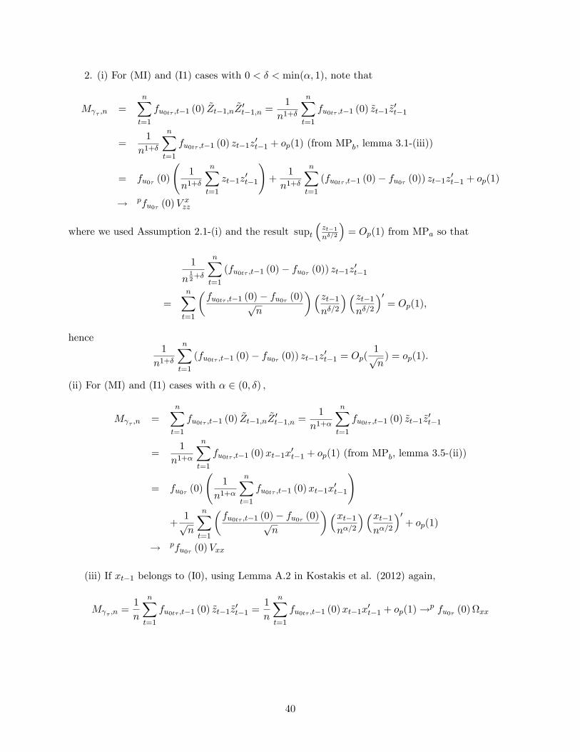
2. (i) For (MI) and (I1) cases with 0 < � < min(�; 1), note that
M � ;n =nXt=1
fu0t� ;t�1 (0) ~Zt�1;n ~Z0t�1;n =
1
n1+�
nXt=1
fu0t� ;t�1 (0) ~zt�1~z0t�1
=1
n1+�
nXt=1
fu0t� ;t�1 (0) zt�1z0t�1 + op(1) (from MPb, lemma 3.1-(iii))
= fu0� (0)
1
n1+�
nXt=1
zt�1z0t�1
!+
1
n1+�
nXt=1
(fu0t� ;t�1 (0)� fu0� (0)) zt�1z0t�1 + op(1)
! pfu0� (0)Vxzz
where we used Assumption 2.1-(i) and the result supt�zt�1n�=2
�= Op(1) from MPa so that
1
n12+�
nXt=1
(fu0t� ;t�1 (0)� fu0� (0)) zt�1z0t�1
=
nXt=1
�fu0t� ;t�1 (0)� fu0� (0)p
n
��zt�1n�=2
��zt�1n�=2
�0= Op(1);
hence1
n1+�
nXt=1
(fu0t� ;t�1 (0)� fu0� (0)) zt�1z0t�1 = Op(1pn) = op(1):
(ii) For (MI) and (I1) cases with � 2 (0; �) ;
M � ;n =
nXt=1
fu0t� ;t�1 (0) ~Zt�1;n ~Z0t�1;n =
1
n1+�
nXt=1
fu0t� ;t�1 (0) ~zt�1~z0t�1
=1
n1+�
nXt=1
fu0t� ;t�1 (0)xt�1x0t�1 + op(1) (from MPb, lemma 3.5-(ii))
= fu0� (0)
1
n1+�
nXt=1
fu0t� ;t�1 (0)xt�1x0t�1
!
+1pn
nXt=1
�fu0t� ;t�1 (0)� fu0� (0)p
n
��xt�1n�=2
��xt�1n�=2
�0+ op(1)
! pfu0� (0)Vxx
(iii) If xt�1 belongs to (I0), using Lemma A.2 in Kostakis et al. (2012) again,
M � ;n =1
n
nXt=1
fu0t� ;t�1 (0) ~zt�1~z0t�1 =
1
n
nXt=1
fu0t� ;t�1 (0)xt�1x0t�1 + op(1)!p fu0� (0)xx
40

3. (i) For (MI) and (I1) cases with 0 < � < min(�; 1),
M�� ;n =nXt=1
fu0t� ;t�1 (0) ~Zt�1;nX0t�1;n
=1
n1+�
nXt=1
fu0t� ;t�1 (0) ~zt�1x0t�1 = fu0� (0)
(1
n1+�
nXt=1
~zt�1x0t�1
)+ op(1) as earlier,
= fu0� (0)
(1
n1+�
nXt=1
zt�1x0t�1 �
C�1z C
n1+�
nXt=1
xt�1x0t�1
)+ op(1) (from MPb, lemma 3.1-(ii))
=)(fu0� (0)
��C�1z
�RdBxJ
c0x +xx
�� C�1z C
�RJcxJ
c0x
�; if � = 1
fu0� (0)��C�1z xx � C�1z CVxx
; if � < � < 1
=
(fu0� (0)
��C�1z
�xx +
RdBxJ
c0x + C
RJcxJ
c0x
�; if � = 1
fu0� (0)��C�1z fxx + CVxxg
�; if � < � < 1
:= fu0� (0)cxz.
and using the fact dJcx = dBx + CJcx from Ito calculus:ZdBxJ
c0x + C
ZJcxJ
c0x =
ZdJcxJ
c0x :
(ii) For (MI) and (I1) cases with � 2 (0; �),
M�� ;n =
nXt=1
fu0t� ;t�1 (0) ~Zt�1;nX0t�1;n
=1
n1+�
nXt=1
fu0t� ;t�1 (0) ~zt�1x0t�1 = fu0� (0)
(1
n1+�
nXt=1
~zt�1x0t�1
)+ op(1) as earlier,
= fu0� (0)
(1
n1+�
nXt=1
xt�1x0t�1 + op(1)
)+ op(1) (from MPb, lemma 3.5-(ii))
=) fu0� (0)Vxx.
(iii) If xt�1 belongs to (I0), using Lemma A.2 in Kostakis et al. (2012) again,
M � ;n =1
n
nXt=1
fu0t� ;t�1 (0) ~zt�1x0t�1 =
1
n
nXt=1
fu0t� ;t�1 (0)xt�1x0t�1 + op(1)!p fu0� (0)xx
To prove Theorem 3.1, I introduce a version of empirical process. Let � 2 RK and
Gn (�) =1
n1+�2
nXt=1
~zt�1� ��u0t� � �0xt�1
�� Et�1
� ��u0t� � �0xt�1
��:
I focus (MI) and (I1) cases here and assume 0 < � < min(�; 1) for documentation purpose; the case
of � 2 (0; �) will be analogous with n� 1+�2 hence omitted. (I0) case is again standard, so omitted.
41

Proof for (ME) predictors will be discussed below (Lemma 7.4).
The stronger normalizer n�1+�2 (than n�
12 ) stabilizes the stronger signal strength of ~zt�1 and
xt�1, and the conditional expectation Et�1 [�] (rather than unconditional expectation) avoids thenonstationarity problem. Thus, the stochastic equicontinuity proof of Bickel (1975) with iid re-
gressors can be modi�ed accordingly. In fact, ~zt�1 and � satisfy condition G and C1 of Bickel
(1975) respectively, hence the analogy of Lemma 4.1 of the paper will hold here. For completeness,
I provide the modi�ed proof.
Lemma 7.3 For a generic constant C > 0;
sup
�kGn (�)�Gn (0)k : k�k �
C
n1+�2
�= op(1)
Proof. WLOG, we assume K = 1: I use the following standard argument:
supfj�j�n�(1+�)=2Cg
jGn (�)�Gn (0)j
= supSj=1;:::;J
fj�j�n�(1+�)=2C(�j)gjGn (�)�Gn (0)j
= maxj=1;:::;J
0@ supfj�j�n�(1+�)=2C(�j)g
jGn (�)�Gn (0)j
1A� max
j=1;:::;J
0@ supfj�j�n�(1+�)=2C(�j)g
jGn (�)�Gn (lj)j+ jGn (lj)�Gn (0)j
1A= max
j=1;:::;J
0@ supfj�j�n�(1+�)=2C(�j)g
jGn (�)�Gn (lj)j
1A+ maxj=1;:::;J
jGn (lj)�Gn (0)j
where�j�j � n�(1+�)=2C (�j) : j = 1; :::; J
is a collection of closed intervals with a length �j whose
union is the original shrinking neighborhood�j�j � n�(1+�)=2C
(see below). lj is the lowest
vertex of each interval. Therefore, we show (i) maxj=1;:::;J jGn (lj)�Gn (0)j = op(1); and (ii)
maxj=1;:::;J
�supfj�j�n�(1+�)=2C(�j)g jGn (�)�Gn (lj)j
�= op(1).
(i) maxj=1;:::;J jGn (lj)�Gn (0)j = op(1):
It su¢ ces to show that
Gn (cn)�Gn (0) = op(1) (7.2)
for cn = c
n1+�2
with any �xed jcj � C; hence a pointwise convergence. I will use the following
argument: if (�nt;Ft) is martingale di¤erence array (mda), and the (predictable) quadratic variationPnt=1E
��nt�
0ntjFt�1
�= op(1); then
nXt=1
�nt = op(1):
42

Let �nt :=1
n1+�2
~zt�1�t where
�t := � (u0t� � cnxt�1)� Et�1 [ � (u0t� � cnxt�1)]� � (u0t� ) + Et�1 [ � (u0t� )]
then
Gn (cn)�Gn (0) =nXt=1
�nt
and by construction �t are mds and �nt are mda.
Note that
�t = 1 (u0t� < 0)� 1 (u0t� < cnxt�1) + Pr (u0t� < cnxt�1jFt�1)� Pr (u0t� < 0jFt�1) :
Given Ft�1; (a) assume cnxt�1 > 0; then
�t = �1 (0 � u0t� < cnxt�1) + Pr (0 � u0t� < cnxt�1jFt�1) ;
and
�2t = 1 (0 � u0t� < cnxt�1) + fPr (0 � u0t� < cnxt�1jFt�1)g2
�2Pr (0 � u0t� < cnxt�1jFt�1) 1 (0 � u0t� < cnxt�1) ;
hence
E��2t jFt�1
�= fPr (0 � u0t� < cnxt�1jFt�1)g f1� Pr (0 � u0t� < cnxt�1jFt�1)g
� fPr (0 � u0t� < cnxt�1jFt�1)g � fu0t� ;t�1(0)cnxt�1 + op(1)
= Op�cnpn�= Op(
1
n�2
) for all t;
thus suptE��2t jFt�1
�= op(1):
It is easy to show for the case (b) cnxt�1 � 0 given Ft�1 in a similar way. Therefore
nXt=1
E��2ntjFt�1
�=
1
n1+�
nXt=1
~z2t�1E��2t jFt�1
�� a:s
�suptE��2t jFt�1
�� 1
n1+�
nXt=1
~z2t�1
!= op(1);
con�rming (7.2).
(ii) maxj=1;:::;J�supfj�j�n�(1+�)=2C(�j)g jGn (�)�Gn (lj)j
�= op(1).
43

For each j;
supfj�j�n�(1+�)=2C(�j)g
jGn (�)�Gn (lj)j
= supfj�j�n�(1+�)=2C(�j)g
����� 1
n1+�2
nXt=1
~zt�1 f1 (ljxt�1 � u0t� < �xt�1)� Pr (ljxt�1 � u0t� < �xt�1jFt�1)g�����
� supfj�j�n�(1+�)=2C(�j)g
1
n1+�2
nXt=1
j~zt�1j 1 (ljxt�1 � u0t� < �xt�1)
+ supfj�j�n�(1+�)=2C(�j)g
1
n1+�2
nXt=1
j~zt�1jPr (ljxt�1 � u0t� < �xt�1jFt�1) :
Now since 1 (ljxt�1 � u0t� < �xt�1) � 1��n�(1+�)=2�jxt�1 � u0t� < n�(1+�)=2�jxt�1
�from the monotonic-
ity,
supfj�j�n�(1+�)=2C(�j)g
1
n1+�2
nXt=1
j~zt�1j 1 (ljxt�1 � u0t� < �xt�1)
!
� 1
n1+�2
nXt=1
j~zt�1j 1��n�(1+�)=2�jxt�1 � u0t� < n�(1+�)=2�jxt�1
�:
Let �nt =1
n1+�2
j~zt�1j 1��n�(1+�)=2�jxt�1 � u0t� < n�(1+�)=2�jxt�1
�; then
nXt=1
Et�1 [�nt] =1
n1+�2
nXt=1
j~zt�1jPr��n�(1+�)=2�jxt�1 � u0t� < �jn
�(1+�)=2xt�1jFt�1�
� 2Mf
n1+�2
nXt=1
j~zt�1j����jn�(1+�)=2xt�1��� = Op (�j) ;
uniformly in �j , where we use that fu0t� ;t�1(�) is bounded above a.s (in the local neighborhood ofzero) by Mf from Assumption 2.1-(ii).
We can also shownXt=1
Et�1��2nt�= op(1);
as before. Thus,
supfj�j�n�(1+�)=2C(�j)g
1
n1+�2
nXt=1
j~zt�1j 1 (ljxt�1 � u0t� < �xt�1)
!= op(1);
Similarly we can show
supfj�j�n�(1+�)=2C(�j)g
1
n1+�2
nXt=1
j~zt�1jPr (ljxt�1 � u0t� < �xt�1jFt�1)!= op(1);
44

con�rming (ii).
Proof of Theorem 3.1. 1. Since I have con�rmed the uniform approximation Lemma 7.3, the
standard result for the extremum estimation with non-smooth criterion function (e.g., Pakes and
Pollard, 1989) holds with a stronger normalization n�1+�2 . Hence, we can show
��IV XQR
1;� � �1;��=
Op
�n�
1+�2
�. Let �1;� = �
IV XQR
1;� within this proof.
Let �� =��1;� � �1;�
�; then from (3.7)
op(1) =1
n1+�2
nXt=1
~zt�1n �
�u0t� �
��1;� � �1;�
�0xt�1
�o=
1
n1+�2
nXt=1
~zt�1� ��u0t� � �� 0xt�1
�� Et�1
� ��u0t� � �� 0xt�1
��� � (u0t� ) + Et�1 ( � (u0t� ))
+
1
n1+�2
nXt=1
~zt�1Et�1� ��u0t� � �� 0xt�1
��+
1
n1+�2
nXt=1
~zt�1 f � (u0t� )g
=1
n1+�2
nXt=1
~zt�1Et�1� ��u0t� � �� 0xt�1
��+
1
n1+�2
nXt=1
~zt�1 f � (u0t� )g+ op(1);
With notation of embedded normalizers,
op(1) =
nXt=1
n~Zt�1;n � (u0t� ) + ~Zt�1;nEt�1
� ��u0t� � �� 0xt�1
��o; (7.3)
and Et�1 ( � (u0t� � �� 0xt�1)) can be expanded around �� = 0 (�1 = �1 (�)), hence
Et�1� ��u0t� � �� 0xt�1
��= Et�1
� ��u0t� � �� 0xt�1
������=0
+@Et�1 [ � (u0t� � �� 0xt�1)]
@�0�
������=0
��+op(�� )
where
Et�1� ��u0t� � �� 0xt�1
��= � � Et�1
�1�u0t� < ��
0xt�1��= � �
Z �� 0xt�1
�1fu0t� ;t�1(s)ds
hence@Et�1 [ � (u0t� � �� 0xt�1)]
@�0�
������=0
= �x0t�1fu0t� ;t�1(0);
thus
Et�1� ��u0t� � �� 0xt�1
��= �x0t�1fu0t� ;t�1(0)�� + op(1):
Putting it back to (7.3),
op(1) = G�;n +
nXt=1
fu0t� ;t�1(0) ~Zt�1;nX0t�1;nn
1+�2
��1;� � �1;�
�;
45

therefore,
n1+�2
��1;� � �1;�
�=�M�� ;n
��1G�;n + op(1);
and the results of Theorem 3.1 for (MI)-(I1) cases follow from Lemma 7.2.
Lemma 7.4 If xt�1 belongs to (ME),
1
n(�^�)R�nn
nXt=1
~zt�1 � (u0t� ) =) CCz�� �N�0; �(1� �) ~Vxx
�;
and (1
n�+(�^�)
Pnt=1 fu0t� ;t�1 (0)R
�nn ~zt�1x0t�1R
�nn
1n�+(�^�)
Pnt=1 fu0t� ;t�1 (0)R
�nn ~zt�1~z0t�1R
�nn
)=) fu0� (0)
~Vxx � CCz��;
where
Cz�� :=
8><>:�C�1z ; if � < �
C�1; if � < �
(C � Cz)�1 ; if � = �
9>=>;Proof. The result directly follows from the proof of Lemma 5.4 and 5.5 in PLb, by replacing u0twith � (u0t� ). Thus, the IVX-QR limit theory in Theorem 3.1 for (ME) case follows by the same
procedure to the earlier proofs - (MI) and (I1) cases.
Proof of Theorem 3.2. Note that
yt� � 01~zt�1 = yt� �� 1 � �1;�
�0~zt�1 � �01;� ~zt�1
= u0t� �� 1 � �1;�
�0~zt�1 + �
01;� (xt�1 � ~zt�1)
= u�0t� �� 1 � �1;�
�0~zt�1
where u�0t� = u0t� + �01;� (xt�1 � ~zt�1). Following the proof of Theorem 2.1, it is straightforward to
show that
n1+(�^�)
2
� IV XQR1;� � �1;�
�=�M � ;n
��1G��;n + op(1);
where
G��;n =nXt=1
~Zt�1;n � (u�0t� ) ;
and it is clear that G��;n = G�;n under H0 : �1;� = 0, leading to
n1+(�^�)
2
� IV XQR1;� � �1;�
�=
�M � ;n
��1G�;n + op(1)
=) N
�0;�(1� �)fu0� (0)
2V�1cxz
�:
46

7.5 Local Power with Estimated Intercepts
Figure 5: c = �5 (n = 250, R = 0:98) with t(4), t(3), t(2) and t(1) innovations.
0 0.01 0.02 0.03 0.04 0.05 0.060
0.2
0.4
0.6
0.8
1Local Power, n=250, C= 5, t(4)
IVXQRIVXmeanCYQNominal Size
0 0.01 0.02 0.03 0.04 0.05 0.060
0.2
0.4
0.6
0.8
1Local Power, n=250, C= 5, t(3)
IVXQRIVXmeanCYQNominal Size
0 0.01 0.02 0.03 0.04 0.05 0.060
0.2
0.4
0.6
0.8
1Local Power, n=250, C= 5, t(2)
IVXQRIVXmeanCYQNominal Size
0 0.01 0.02 0.03 0.04 0.05 0.060
0.2
0.4
0.6
0.8
1Local Power, n=250, C= 5, t(1)
IVXQRIVXmeanCYQNominal Size
Figure 6: c = �25 (n = 250; R = 0:9) with t(4), t(3), t(2) and t(1) innovations.
0 0.02 0.04 0.06 0.08 0.1 0.120
0.2
0.4
0.6
0.8
1Local Power, n=250, C= 25, t(4)
IVXQRIVXmeanCYQNominal Size
0 0.02 0.04 0.06 0.08 0.1 0.120
0.2
0.4
0.6
0.8
1Local Power, n=250, C= 25, t(3)
IVXQRIVXmeanCYQNominal Size
0 0.02 0.04 0.06 0.08 0.1 0.120
0.2
0.4
0.6
0.8
1Local Power, n=250, C= 25, t(2)
IVXQRIVXmeanCYQNominal Size
0 0.05 0.1 0.15 0.20
0.2
0.4
0.6
0.8
1t(1)
IVXQRIVXmeanCYQNominal Size
47

7.6 Diagnostic Tests for Comovement between Persistent Predictors
Table 9: Diagnostic Tests for Comovement (full sample period: Jan 1927 to Dec 2005)
(d/p, tbl) correlation Johansen tests for cointegration
-0.16 maximum rank trace statistics 5% critical value
0 11.76* 15.41
1 3.46 3.76
(d/p, dfy) correlation Johansen tests for cointegration
0.44 maximum rank trace statistics 5% critical value
0 20.74 15.41
1 2.99* 3.76
(d/e, tbl) correlation Johansen tests for cointegration
-0.52 maximum rank trace statistics 5% critical value
0 21.54 15.41
1 7.46 3.76
(d/e, dfy) correlation Johansen tests for cointegration
0.56 maximum rank trace statistics 5% critical value
0 33.98 15.41
1 7.57 3.76
(d/p, b/m) correlation Johansen tests for cointegration
0.82 maximum rank trace statistics 5% critical value
0 23.74 15.41
1 3.82 3.76
(d/e, b/m) correlation Johansen tests for cointegration
0.29 maximum rank trace statistics 5% critical value
0 21.82 15.41
1 6.78 3.76
(tbl, b/m) correlation Johansen tests for cointegration
0.07 maximum rank trace statistics 5% critical value
0 18.37 15.41
1 7.20 3.76
(dfy, b/m) correlation Johansen tests for cointegration
0.52 maximum rank trace statistics 5% critical value
0 25.79 15.41
1 8.64 3.76
48

Table 10: Diagnostic Tests for Comovement (subperiod: Jan 1952 to Dec 2005)
(b/m, d/p) correlation Johansen tests for cointegration
0.88 maximum rank trace statistics 5% critical value
0 10.34* 15.41
1 2.85 3.76
(b/m, dfy) correlation Johansen tests for cointegration
0.47 maximum rank trace statistics 5% critical value
0 32.86 15.41
1 3.13* 3.76
(b/m, e/p) correlation Johansen tests for cointegration
0.89 maximum rank trace statistics 5% critical value
0 9.70* 15.41
1 1.95 3.76
(b/m, tbl) correlation Johansen tests for cointegration
0.50 maximum rank trace statistics 5% critical value
0 14.89* 15.41
1 2.00 3.76
(d/p, tbl) correlation Johansen tests for cointegration
0.35 maximum rank trace statistics 5% critical value
0 15.68 15.41
1 2.05* 3.76
(dfy, tbl) correlation Johansen tests for cointegration
0.58 maximum rank trace statistics 5% critical value
0 40.87 15.41
1 5.77 3.76
(e/p, tbl) correlation Johansen tests for cointegration
0.53 maximum rank trace statistics 5% critical value
0 16.74 15.41
1 3.75* 3.76
8 References
Bickel, P.J (1975). "One-Step Huber Estimates in the Linear Model," Journal of the American
Statistical Association, 70(350), pp.428-434.
Campbell, J. and S. Thompson (2008). "Predicting excess stock returns out of sample: can
anything beat the historical average?", Review of Financial Studies, 21(4), pp. 1509-1531.
Campbell, J. and M. Yogo (2006). "E¢ cient tests of stock return predictability," Journal of
Financial Economics, 81(1), 27-60.
49

Cavanagh, C., G. Elliott. and J.Stock (1995). "Inference in models with nearly integrated regres-
sors," Econometric Theory, 11(05), 1131-1147.
Cenesizoglu, T and A. Timmermann (2008). "Is the distribution of stock returns predictable?
Unpublished Manuscript, HEC Montreal and UCSD.
Chernozhukov, V (2005). "Extremal quantile regression," Annals of Statistics, 33, 806-839.
Chernozhukov, V. and I. Fernandez-Val (2011). "Inference for extremal conditional quantile mod-
els, with an application to market and birthweight risks," Review of Economic Studies, 78(2),
559-589.
Cont, R (2001), "Empirical properties of asset returns: stylized facts and statistical issues",
Quantitative Finance, 1:2, 223-336
Elliott, G. and J.H. Stock (1994). "Inference in time series regression when the order of integration
of a regressor is unknown," Econometric Theory, 10(3-4), 672-700.
Embrechts, P., Kluppelberg, C. and Mikosch, T (1997). Modelling Extremal Events, Springer
Verlag, Berlin.
Fama, E. and K. French (1993). "Common risk factors in the returns on stocks and bonds, "
Journal of Financial Economics, 33(1), 3-56.
Goyal, A and I. Welch (2008). " A comprehensive look at the empirical performance of equity
premium prediction," Review of Financial Studies, 21(4), 1455-1508.
Hall, P. and C.C. Heyde (1980). Martingale Limit Theory and its Application. Academic Press.
Jansson, M. and M. Moreira (2006). "Optimal inference in regression models with nearly inte-
grated regressors," Econometrica, 74(3), 681-714.
Johansen, S (1988), "Statistical analysis of cointegration vectors," Journal of Economic Dynamics
and Control, 12(2-3), pp. 231-254.
Knight, K (1989). "Limit theory for autoregressive-parameter estimates in an in�nite-variance
random walk," Canadian Journal of Statistics, 17, 261-278.
Koenker, R (2005). Econometric Society Monographs: Quantile Regression. Cambridge Press.
Koenker, R and G. Basset (1978). "Regression quantiles," Econometrica 46, 33-49.
Kostakis, A., A. Magdalinos and M. Stamatogiannis (2010). "Robust econometric inference for
stock return predictability," Unpublished Manuscript, University of Nottingham.
Magdalinos, T. and P. C. B Phillips (2009a). �Limit theory for cointegrated systems with moder-
ately integrated and moderately explosive regressors�. Econometric Theory, 25, 482-526.
50

Magdalinos, T. and P. C. B Phillips (2009b). �Econometric inference in the vicinity of unity�.
CoFie Working Paper (7), Singapore Management University.
Maynard A., K. Shimotsu and Y. Wang (2011). "Inference in predictive quantile regressions,"
Unpublished Manuscript.
Pakes, A. and D. Pollard (1989). "Simulation and the asymptotics of optimization estimators,"
Econometrica 57(5), pp.1027-1057.
Phillips, P. C. B. (1995). �Fully modi�ed least squares and vector autoregression,�Econometrica
63(5), 1023�1078.
Phillips, P. C. B (2012), "On con�dence Intervals for autoregressive roots and predictive regres-
sion," Unpublished Manuscript.
Phillips, P. C. B. (1989), "Partially identi�ed econometric models," Econometric Theory, 5(2),
pp. 181-240
Phillips, P. C. B. (1987). �Towards a uni�ed asymptotic theory for autoregression,�Biometrika
74, 535�547
Phillips, P. C. B. and B. Hansen (1990). �Statistical inference in instrumental variables regression
with I(1) processes,�Review of Economic Studies, 57(1), 99.
Phillips, P. C. B and J.H. Lee (2012a), "Predictive regression under various degrees of persistence
and robust long-horizon regression," Unpublished Manuscript.
Phillips, P. C. B and J.H. Lee (2012b), "Robust econometric inference with mixed integrated and
mildly explosive regressors," Unpublished Manuscript.
Phillips, P. C. B. and T. Magdalinos (2007a), "Limit theory for moderate deviations from a unit
root," Journal of Econometrics 136, 115-130.
Phillips, P. C. B. and T. Magdalinos (2007b), "Limit theory for moderate deviations from a unit
root under weak dependence," in G. D. A. Phillips and E. Tzavalis (Eds.) The Re�nement
of Econometric Estimation and Test Procedures: Finite Sample and Asymptotic Analysis.
Cambridge: Cambridge University Press, pp.123-162.
Phillips, P. C. B. and V. Solo (1992). �Asymptotics for linear processes�, The Annals of Statistics,
pp. 971-1001.
Pollard, D. (1991)."Asymptotics for least absolute deviation regression estimators," Econometric
Theory, 7(2), pp. 186-199.
Stock, J. (1991). "Con�dence intervals for the largest autoregressive root in US macroeconomic
time series," Journal of Monetary Economics, 28(3), 435-459.
51

Xiao, Z (2009). "Quantile cointegrating regression," Journal of Econometrics, 150, 248-260.
52