i

Predictive Modelling Applied to Propensity to

Buy Personal Accidents Insurance Products

Esdras Christo Moura dos Santos

Internship report presented as partial requirement for

obtaining the Master’s degree in Advanced Analytics

i

Title: Predictive Models Applied to Propensity to Buy Personal Accidents Insurance Products

Student: Esdras Christo Moura dos Santos MAA

20

17

i

ii

NOVA Information Management School

Instituto Superior de Estatística e Gestão de Informação

Universidade Nova de Lisboa

PREDICTIVE MODELLING APPLIED TO PROPENSITY TO BUY

PERSONAL ACCIDENTS INSURANCE PRODUCTS

by

Esdras Christo Moura dos Santos

Internship report presented as partial requirement for obtaining the Master’s degree in

Advanced Analytics

Advisor: Mauro Castelli

iii

February 2018

DEDICATION

Dedicated to my beloved family.

iv

ACKNOWLEDGEMENTS

I would like to express my gratitude to my supervisor, Professor Mauro Castelli of Information

Management School of Universidade Nova de Lisboa for all the mentoring and assistance. I also

want to show my gratitude for the data mining team at Ocidental, Magdalena Neate and Franklin

Minang. I deeply appreciate all the guidance, patience and support during this project.

v

ABSTRACT

Predictive models have been largely used in organizational scenarios with the increasing

popularity of machine learning. They play a fundamental role in the support of customer acquisition

in marketing campaigns. This report describes the development of a propensity to buy model for

personal accident insurance products. The entire process from business understanding to the

deployment of the final model is analyzed with the objective of linking the theory to practice.

KEYWORDS

Predictive models; data mining; supervised learning; propensity to buy; logistic regression; decision

trees; artificial neural networks; ensemble models.

vi

INDEX

1. Introduction AND Motivation ........................................................................................ 1

2. Part I.............................................................................................................................. 2

2.1. Data Mining Processes .......................................................................................... 2

2.1.1. CRISP-DM ........................................................................................................ 2

2.1.2. SEMMA ........................................................................................................... 4

2.2. Predictive Models .................................................................................................. 6

2.2.1. Logistic Regression ......................................................................................... 7

2.2.2. Decision Trees ................................................................................................ 9

2.2.3. Artificial Neural Networks ............................................................................ 13

2.2.4. Ensemble Models ......................................................................................... 16

2.3. Predictive Models Evaluation .............................................................................. 17

2.3.1. Performance Measure of Binary Classification ............................................ 17

3. Part II........................................................................................................................... 24

3.1. Methodology ....................................................................................................... 24

3.1.1. Business Understanding ............................................................................... 24

3.1.2. Data Understanding ..................................................................................... 25

3.1.3. Data Preparation .......................................................................................... 26

3.1.4. Modelling ...................................................................................................... 31

3.1.5. Final Evaluation and Results ......................................................................... 45

4. Conclusions and Deployment ..................................................................................... 50

4.1. Limitations and Recommendations for Future Works ........................................ 50

Appendix.......................................................................................................................... 52

Bibliography..................................................................................................................... 77

vii

LIST OF FIGURES

Figure 1 - CRISP-DM ................................................................................................................... 3

Figure 2 - SEMMA ....................................................................................................................... 4

Figure 3 – Sigmoid Function. ...................................................................................................... 8

Figure 4 – Decision Tree Representation. .................................................................................. 9

Figure 5 – Logworth function. .................................................................................................. 11

Figure 6 – Entropy of a Binary Variable .................................................................................... 12

Figure 7 - Artificial Neural Network Representation ............................................................... 13

Figure 8 – Sigmoid Activation Function. ................................................................................... 15

Figure 9 – ROC Curve ................................................................................................................ 22

Figure 10 - Lift Chart ................................................................................................................. 23

Figure 11 – Distribution of Idade_Adj ...................................................................................... 27

Figure 12 – Distribution of No_Claims_Ever_NH ..................................................................... 28

Figure 13 – Sample Distribution of Idade-Adj .......................................................................... 29

Figure 14 – Correlation Matrix ................................................................................................. 30

Figure 15 – Modelling Process. ................................................................................................ 32

Figure 16 - Regression Models ................................................................................................. 33

Figure 17 – Regression model Average Squared Error ............................................................ 34

Figure 18 – Regression ROC Curve ........................................................................................... 35

Figure 19 – Regression Misclassification Rate ......................................................................... 36

Figure 20 – Decision Tree Models ............................................................................................ 36

Figure 21 – Decision Tree Average Squared Error ................................................................... 38

Figure 22 – Decision Tree Misclassification Rate ..................................................................... 39

Figure 23 – Decision Tree ROC curves. ..................................................................................... 39

viii

Figure 24 – Decision Tree Structure ......................................................................................... 40

Figure 25 – Artificial Neural Networks Models ........................................................................ 41

Figure 26 – Artificial Neural Network ASE with all inputs. ....................................................... 41

Figure 27 – Artificial Neural Network Average Squared Error. ................................................ 42

Figure 28 – Artificial Neural Network Misclassification Rate. .................................................. 42

Figure 29 – Artificial Neural Network ROC curves. .................................................................. 43

Figure 30 – Posterior Probabilities ........................................................................................... 44

Figure 31 – Ensemble Model ROC Curves ................................................................................ 45

Figure 32 – Cummulative Lift Comparison ............................................................................... 46

Figure 33 – Histogram of Unadjusted Probabilities. ................................................................ 48

Figure 34 – Histogram of Adjusted Probabilities. .................................................................... 48

Figure 35 – Decision Tree Structure. ........................................................................................ 76

ix

LIST OF TABLES

Table 1 – CRISP-DM & SEMMA .................................................................................................. 5

Table 2 – Confusion Matrix ...................................................................................................... 17

Table 3 – Data Partition. ........................................................................................................... 29

Table 4 – Regression Model Coefficients. ................................................................................ 34

Table 5 – Regression Model Evaluation ................................................................................... 35

Table 6 – Decision Tree Configuration ..................................................................................... 38

Table 7 – Decision Tree Evaluation .......................................................................................... 38

Table 8 – Artificial Neural Network Evaluation ........................................................................ 42

Table 9 – Ensembel Model evaluation ..................................................................................... 44

Table 10 – Training Performance Comparison. ........................................................................ 46

Table 11 – Validation Performance Comparison. .................................................................... 46

Table 12 – Probabilities statistics. ............................................................................................ 47

Table 13 – Test Data Cumulative Lift. ...................................................................................... 49

Table 14 –List of Input Variables .............................................................................................. 59

Table 15 – Variables excluded .................................................................................................. 61

Table 16 – Data set quantitative var. descriptive statistics. .................................................... 67

Table 17 –Sample quantitative variables descriptive statistics ............................................... 73

Table 18 – Statistics Comparison ............................................................................................. 75

1

1. INTRODUCTION AND MOTIVATION

The Master’s degree in Advanced Analytics at NOVA IMS offers the option of writing a thesis or developing a practical project through an internship with the purpose of applying the theory studied during the first year of the master to earn the degree in Advanced Analytics. The aim of this report is to describe the development of a predictive model for understanding the propensity to buy a Personal Accident Insurance product at Ocidental Seguros.

One of the main reasons for studying predictive models is due to the enormous amount of data that business produce today. As a result, the need to process this information to gain insights and make improvements has become fundamental to stay competitive. The insurance industry is an example of an industry that has taken advantage of analytics. One of the main objectives of an insurance company, besides increasing its client base, is to increase the number of policies held by its clients. Data mining techniques are applied to achieve this goal, especially predictive modelling.

Predictive modelling is used in the marketing of many products and services. Insurers can use predictive models to analyze the purchasing patterns of insurance customers in addition to their demographic attributes. This information can then be used to increase the marketing success rate, which is a measure of how often the marketing function generates a sale for each contact made with a potential customer. Predictive analytics used to analyze the purchasing patterns may allow the agents to focus on the customers who are more likely to buy, thereby increasing the success of marketing campaigns.

This report is structured in two main parts. Part I is focused on the literature review and explanation of the predictive modelling process, while Part II comprises the application of the theory outlined in the first section relating it to a practical business scenario. Additional business specifications are described to achieve this goal throughout the development of a predictive model applied to a propensity to buy personal accident insurance products.

2

2. PART I

Developing a predictive model it is one of the steps that are encompassed in the data mining

process. As such, Part I of this report starts with a brief explanation of the data mining process and

proceeds with the explanation of the predictive modelling task.

2.1. DATA MINING PROCESSES

Before analyzing the techniques applied to predictive modelling, it is crucial to have an overview

of the whole data mining process. Two main methodologies with similar approaches are presented

below. Their applications are detailed in the practical section.

2.1.1. CRISP-DM

CRISP-DM1 (Olson & Delen, 2008) is a process widely used by the industry members. This

process consists of six phases that can be partially cyclical (Figure 1):

1 Cross-Industry Standard Process for data mining

3

Figure 1 - CRISP-DM

Business Understanding: Most of the data mining processes aim to provide a solution to a

problem. Having a clear understanding of the business objectives, assessment of the current

situation, data mining goals and the plan of development are fundamental to the achievement

of the objectives.

Data Understanding: Once the business context and objectives are covered, data

understanding considers data requirements. This step encompasses data collection and data

quality verification. At the end of this phase, a preliminary data exploration can occur.

Data Preparation: In this step, the data cleaning techniques are applied to prepare the data to

be used as input for the modelling phase. A more thorough data exploration is carried during

this phase providing an opportunity to see patterns based on business understanding.

Modelling: The modelling stage uses data mining tools to apply algorithms suitable to the task

at hand. The next section of this report is dedicated to detail a few techniques applied during

this step.

4

Evaluation: The evaluation of the models is done by taking into account several evaluation

metrics and comparing the performance of the models built during the modelling phase. This

step should also consider the business objectives when choosing the final model.

Deployment: The knowledge discovered during the previous phases need to be reported to

the management and be applied to the business environment. Additionally, the insights gained

during the process might change over time. Therefore, it is critical that the domain of interest

be monitored during its period of deployment.

2.1.2. SEMMA

In addition to CRISP-DM, another well-known methodology developed by the SAS Institute is the

SEMMA2 process (Olson & Delen, 2008) shown in Figure 2. Each phase of the process is described

below:

Figure 2 - SEMMA

Sample: Representative samples of the data are extracted to improve computational

performance and reduce processing time. It is also appropriately partition the data into

training validation and test data for better modelling and accuracy assessment;

Explore: Through the exploration of the data, data quality is assured and insights are gained

based on visualization and summary statistics. Trends and relationship can also be identified in

this step;

Modify: Based on the discoveries during the exploration phase it might be necessary to

exclude, create and transform the variables in the data set before the modelling phase. It is

2 Sample, Explore, Modify, Model and Assess

5

also important to verify the presence of outliers, which can damage the performance of the

models;

Model: During this phase, the search task of finding the model that best accomplish the goals

of the process is performed. The models might serve different purposes, but are generally

classified into two groups. The first concerns the descriptive models, also known as

unsupervised learning models, this set of techniques aim to describe the structure and/or

summarize the data. Clustering and association rules are examples of descriptive/unsupervised

algorithms. The second group comprehends the predictive models, also known as supervised

learning models, the objective of these models is to create structures that can predict with

some degree of confidence the outcome of an event based on a set of labeled examples. A

more precise definition is given in the next section;

Assess: In this final step of the data mining process the user assesses the model to estimate

how well it performs. A common approach to assess the performance of the model is to apply

the model to a portion of the data that was not used to build the model. Then, an unbiased

estimative of the performance of the model can be analyzed.

The two data mining processes mentioned give an overview of the development of a predictive

model. These two approaches were shown because the CRISP-DM relates the data mining process

with the business context, while SEMMA details the technical steps needed to build a model once the

business objectives have been defined. The table below (Table 1) shows the similarity between each

phase of both processes.

CRISP-DM SEMMA

Business Understanding

-

Data Understanding Sample Explore

Data Preparation Modify

Modelling Model

Evaluation Assessment

Deployment -

Table 1 – CRISP-DM & SEMMA

After giving an overview of the data mining process, we can now concentrate on the modelling

part of the process. The next section is dedicated to describing the predictive models used during the

practical section.

6

2.2. PREDICTIVE MODELS

As mentioned in the previous section, the modelling step of a project can have two approaches

according to the objective, a predictive or descriptive modelling analysis. In this section, the

predictive models discussed are focused on a binary classification problem since it is the scenario of

the practical section of this report. A few concise definitions of predictive modelling are presented

below.

“Predictive modeling is a name given to a collection of mathematical techniques having in

common the goal of finding a mathematical relationship between a target, response, or “dependent”

variable and various predictor or “independent” variables with the goal in mind of measuring future

values of those predictors and inserting them into the mathematical relationship to predict future

values of the target variable”

(Dickey, D. A., 2012, Introduction to Predictive Modeling with Examples)

“Predictive Analytics is a broad term describing a variety of statistical and analytical techniques

used to develop models that predict future events or behaviors. The form of these predictive models

varies, depending on the behavior or event they are predicting. Most predictive models generate a

score (a credit score, for example), with a higher score indicating a higher likelihood of the given

behavior or event occurring”

(Nyce C., 2007, Predictive Analytics White Paper)

“Predictive modelling (also known as supervised prediction or supervised learning) starts with a

training data set. The observations in a training data set are known as training cases (also called

training examples, instances, or records). The variables are called inputs (also known as predictors,

features, explanatory variables, or independent variables) and targets (also known as response,

outcome, or dependent variable). For a given case, the inputs reflect your state of knowledge before

measuring the target”

(Christie et al., 2011, Applied Analytics Using SAS Enterprise Miner)

The definitions above state that predictive model is a relationship between a target variable and

a set of inputs. This relationship is detected by analyzing the training data set. Additionally, other

data sets are used to improve the performance of a predictive model and its ability to generalize for

cases that are not in the training data, validation data and test data address this problem. The

former is used to evaluate the error of the model and gives an indication when to stop training to

improve its generalization, while the latter is used exclusively to give an unbiased estimation of the

performance of the model.

Regardless of the predictive model, it must fulfill the following requirements:

Provide a rule to transform a measurement into a prediction;

Be able to attribute importance among useful input from a vast number of candidates;

Have a mean to adjust its complexity to compensate for noisy training data.

7

In the following subsections, the three most commonly used predictive modelling methods and

a combination of them are detailed, considering the implementations provided by the SAS EM3 data

mining tool.

2.2.1. Logistic Regression

Logistic Regression is a type of regression applied when the target variable is a dichotomous

(binary) variable and it belongs to a class of models named GLM (generalized linear models). The goal

of logistic regression is to estimate the probability of an event conditional to a set of input variables

(Hosmer, Lemeshow, 1989). After estimating the probability of an instance, the classification of it as

event or non-event can be made.

As mentioned previously, the target variable can take value 1 with probability of success p or

value 0 with probability (1-p). Variables with this nature follow a Bernoulli distribution, which is a

special case of the Binomial distribution when the number of trials is equal to 1. The relationship

between the target variable and the inputs is not a linear function in a logistic regression, a link

function denominated logit is used to establish the association between the inputs and the target

variable.

𝑙𝑜𝑔𝑖𝑡(𝑝) = ln (𝑝

1 − 𝑝)

However, the probability p is unknown, it has to be estimated conditional to the inputs. As a

result, the following equation describes the relation between the probability and the inputs:

ln (𝑝

1 − 𝑝) = �̅�𝑇�̅�

With some algebra, the relationship can be simplified as the equation below.

�̂� = 1

1 + 𝑒−�̅�𝑇�̅�

The term on the right side of the equality is known as logistic function. If we define u = �̅�𝑇�̅�, the

relationship between the sigmoid function f and u can be visualized in Figure 3. Large values of u give

high values of the dependent variable (�̂�=f(u)), while high negative values of u give values of the

dependent variable close to 0.The values of f(u) are interpreted as the estimated posterior

probabilities

3 SAS Enterprise Miner

8

Figure 3 – Sigmoid Function.

The goal of logistic regression is to correctly predict the category of the outcome for individual

cases using the most parsimonious model. The coefficients �̅� are estimated through maximum

likelihood, but the choice of the most parsimonious model is subject to a variable selection method.

Essentially, the choice of an adequate model is based on the significance of the coefficients

associated with the input variable. The first possibility of variable selection method is the Backwards

Selection, with this option the training begins with all candidate inputs and removes the inputs until

only inputs with p-values determined by an F-test or t-test are lower than a predefined significance

level, typically 0.05. The Forward Selection method starts with no input variable, the inputs are

included in the model sequentially based on the significance of each variable. At each iteration, the

variable with the lowest p-value lower than the significance level is included in the model. This

process is repeated until there are no more variables that fulfill this entry criterion. Lastly, the

Stepwise Selection starts as Forward Selection, but the removal of inputs is possible if an inputs

becomes non-significant through the iterations. This process continues until no variable meets the

entry criterion or other stop condition is reached.

The final model, depending on the selection method, can also be evaluated on the validation

data. An alternative for not relying exclusively on the statistical significance of the model consists of

evaluating the model at each step of the model selection. Then, the model with the highest

performance on the validation set is chosen regardless if any of the inputs is significant or not.

9

2.2.2. Decision Trees

Decision Trees are among the most popular predictive algorithms due to their structure and

interpretability. Additionally, they are applied in various fields, ranging from medical diagnosis to

credit risk.

2.2.2.1. Decision Trees Representation

Decision trees classify instances by sorting them down from the root node to a leaf node. Each

node in the tree test an if-else rule of some variable of an observation, and each branch descending

from that node corresponds to one of the possible values of this attribute. This process is repeated

until a leaf node is reached. Figure 4 represents this procedure.

Figure 4 – Decision Tree Representation.

The first rule, at the base (top) of the tree, is named the root node. Subsequent rules are named

interior nodes. Nodes with only one connection are leaf nodes. A tree leaf provides a classification

and an estimate (for example, the proportion of success events). A node, which is divided into sub-

nodes is called parent node of sub-nodes, whereas sub-nodes are the child of parent node (Rokach &

Maimon, 2015).

2.2.2.2. Growing a Decision Tree

The growth of a decision tree is determined by a split-search algorithm. To measure the

goodness of a split different functions can be used, the most known are Entropy and Chi-Square, both

approaches are available in SAS EM.

10

2.2.2.3. CHAID (Chi-Square Automatic Interaction Detection)

The splitting criterion in CHAID is based on the p-value of the Pearson Chi-Square of

Independence, which defines the null hypothesis as the absence of a relation between the

independent variable and the target variable. By selecting the input variable with the lowest

significant p-value, the algorithm is intrinsically selecting the variable that has the highest association

with the target variable at each step (Ritschard, 2010).

This algorithm has two steps:

1) Merge step: The aim of this step is to group the categories that are not significantly different

for each input variable. For example, if a nominal variables X1 has levels c1, c2 and c3. Then, a

chi-square test for each pair of levels is computed. The test with the highest p-value indicates

what levels should be aggregated. This process repeats until only significantly aggregated

levels are eligible for splitting;

2) Split search: In this step, each input resulting from the previous step is considered for split.

Then, for each input, the algorithm searches for the best split. That is, the point (or the classes

for nominal variables) that maximizes the logworth function. The logworth of a split is a

function of the p-value associated with the Chi-Square test of the input obtained in the

previous step and the target variable, it is given by the following equation:

𝑙𝑜𝑔𝑤𝑜𝑟𝑡ℎ = − log10 (𝐶ℎ𝑖 − 𝑆𝑞𝑢𝑎𝑟𝑒𝑑 𝑝 − 𝑣𝑎𝑙𝑢𝑒)

The input that provides the highest logworth is selected for split. Then, another split is

calculated if no termination criterion is met.

The termination criteria in CHAID trees are the following:

1) No split produce a logworth higher than the threshold defined;

2) Maximum tree depth is reached;

3) Minimum number of cases in a node for being a parent node is reached, so it cannot split any

further;

4) Minimum number of cases in a node for being a child node is reached.

11

In SAS EM the default value for comparison of the logworth is 0.7, which is associated with a p-

value of 0.2. Then, if an input has a logworth higher than 0.7, it is eligible to be used in a split. The

logworth function can be analyzed in Figure 5, the dashed line represents the threshold.

Figure 5 – Logworth function.

2.2.2.4. Impurity Based Trees

Differently from the Chi-Square splitting criterion, which is based on statistical hypothesis

testing, the entropy reduction criterion is related to information theory. Entropy measures the

impurity of a sample. The entropy function E of a collection S in a c class classification is defined as:

E(S) = − ∑ 𝑝𝑖𝑐𝑖=1 × 𝑙𝑜𝑔2(𝑝𝑖)

Where 𝑝𝑖 is the proportion of S belonging to class 𝑖. For a binary target variable S, the entropy

function is displayed in Figure 6 and it is computed as:

E(S) = −[𝑝 ∗ 𝑙𝑜𝑔2(𝑝) + (1 − 𝑝) ∗ 𝑙𝑜𝑔2(1 − 𝑝)]

12

Figure 6 – Entropy of a Binary Variable

Figure 6 shows the variation of the entropy for a binary target variable. The maximum is reached

when there is no distinction for the target variable, which corresponds to a 50%-50% proportion of

event and non-event. As a result, the aim of the algorithm is to find the split that minimizes the

entropy, which provides the largest difference in proportion between the target levels.

Entropy measures the impurity of a split in the training examples. To define the effectiveness of

a variable in classifying the training data the algorithm uses a measure called information gain (Gain),

which is the reduction in entropy caused by the partitioning of the examples according to an input

variable (Mitchel, 1997). The Gain relative to a collection S and an input A is defined as:

Gain(S, A) ≡ Entropy(S) - ∑|𝑆𝑣|

|𝑆|𝑣 ∈𝑉𝑎𝑙𝑢𝑒𝑠(𝐴) Entropy(𝑆𝑣)

Values(A) is the set of all possible values for input A, and 𝑆𝑣 is the subset of S for which input A

has value 𝑣. This measure is computed for each variable. Then, the variable that gives the largest

Gain is chosen to split. It is important to notice that the initialization of the algorithm computes the

initial entropy of the system by computing the entropy of the target variable. The previous formulae

presented in this section assume nominal features, but decision trees use information gain for

splitting on numeric features as well. To do so, a common practice is to test various splits that divide

the values into groups greater than or less than a numeric threshold. This process binds the numeric

features, allowing the information gain to be calculated as usual.

13

The stopping criterion is reached when there is no possible increase in information gain for a

split in a branch or all training examples belong to the same target class. Because information gain

criteria lack the significance threshold feature of the chi-square criterion, they tend to grow

enormous trees. Pruning and selection of a tree complexity are based on validation data.

2.2.3. Artificial Neural Networks

Neural Networks are a class of models that belong to a set called black box methods because the

mechanism that transforms the inputs into the outputs is obfuscated by an imaginary box (Lantz,

2013). However, the mechanism behind neural networks is derived from the knowledge of how a

biological brain responds to stimuli from sensory inputs (Mitchel, 1997).

Figure 7 - Artificial Neural Network Representation

Figure 7 illustrates an artificial neural network, the type of neural networks shown has three

layers. The first layer is called input layer (the inputs are 𝑥1, 𝑥2, and 𝑥3), the second layer is the

hidden layer and the third layer is the output layer. The connections between the layers a𝑘𝑖 are called

weights, the superscripts identify the layer, while the subscripts show the number of the weight. In

each neuron in the hidden layer and output layer an activation function f is applied to the linear

combination of weights and inputs as follow:

𝑦(𝑥) = 𝑓 (∑ a𝑖𝑥𝑖 + a𝑛+1𝑏𝑖𝑎𝑠

𝑛

𝑖=1

)

14

The elements of a neural network are described below:

Network topology: The topology of network describes the number of neurons in the model as

well as the number of layers and the manner they are connected;

Activation function: This is a function that transforms a neuron’s combined input signals into

a single output to be transmitted further in the network;

Training algorithm: The training algorithm specifies how connection weights are set in order to

inhibit or excite neurons in proportion to the input signal.

2.2.3.1. Network Topology

As it might expected, the number of layers and neurons increase the complexity of the neural

network and the ability of the network to adapt to the training data more accurately. As a result,

adding too many hidden layers or neurons might lead to overfitting. There is no general rule to

determine the number of hidden neurons or layers. However, the evaluation on the validation data

can be used to indicate an appropriate number of hidden neurons and layers.

In this section, also in the practical section, the only network topology considered is the feed

forward topology, which implies that the neural network has three layers, the input layer, the hidden

layer and the output layer. Moreover, all the neurons in a layer are connected to all the other

neurons in the subsequent layer, except the bias term. Figure 7 shows an example of a feed forward

network.

2.2.3.2. Activation Function

The activation function is the tool that enables the information pass through the network. A

common activation function is the sigmoid activation function because of its properties such as non-

linear, monotonically increasing, easily differentiable and bounded between 0 and 1 (Anthony, 2001),

as shown in Figure 8.

15

Figure 8 – Sigmoid Activation Function.

2.2.3.3. Training Algorithm

The topology of a network itself has not learned anything. To gain knowledge, it must be trained

on the input data. As the neural network processes the input data, connections between the neurons

are strengthened or weakened. This process is computationally expensive, only after the

development of efficient algorithms to update the weights neural networks started being applied. An

algorithm commonly used is the backpropagation algorithm. This algorithm has two main phases:

Forward phase: The neurons are activated in sequence from the input layer to the output

layer, applying each neuron’s weights and activation function along the way. When iteration

reaches the output layer, an output signal is produced;

Backward phase: The network’s output signal resulting from the forward phase is compared to

the true value in the training data. The difference between the network’s output signal and the

true value results in an error that is propagated backward in the network to modify the

connection weights between neurons and reduce future errors.

Over the iterations of forward and backward phases, the weights are updated in order to reduce

the error. The amount by which each weight changed is determined by a technique named gradient

descent. This technique uses the derivative of each neuron’s activation function to determine the

16

direction that each weight should be updated by an amount known as the learning rate to reduce the

error.

A noticeable disadvantage of neural networks, besides being computationally expensive, is the

absence of a variable selection mechanism, which can cause premature overfitting. Other

weaknesses of neural networks can be identified, such as the tendency to overfitting and the

impossibility of interpretation.

2.2.4. Ensemble Models

Ensemble models have many advantages (Lantz, 2015), some of them are:

Generalization: Since the output of several models are incorporated into a single final

prediction, the bias of each model are attenuated;

Improved performance on massive or small datasets: Many models run into memory or

complexity limitations. Then, a possible strategy to overcome this issue is to train several small

models than a single full model. Oppositely, in small data sets ensemble models provide a

good performance because resampling methods such as bootstrapping are inherently a part of

many ensemble designs.

Synthesize data from distinct domains: Since there is no one-size-fits-all learning algorithms,

the ensemble’s ability to incorporate evidence from multiple types of models with data drawn

from different domains.

Ensemble methods are based on the idea that by combining multiple learners, a strong learner

is created. Two main considerations have to be taken into account when building an ensemble

model:

1) The differences in the models selection and creation;

2) The method of combining the prediction of the different models into a single prediction.

To address the first consideration, it must be decided if the models are going to be trained with

different partitions of the data or the whole data set, and if all the inputs are going to be used for all

the models. These decisions are made by an allocation function. The aim of the allocation function is

to increase diversity by artificially varying the input data to bias the resulting learners, even if they

are of the same type. If the ensemble already includes a diverse set of algorithms such as neural

networks, decision trees and regression models, the allocation function might pass the data on to

each algorithm relatively unchanged.

The second issue is resolved by defining a combination function that manages how the output of

each one of the models are combined. For example, the average of the posterior probabilities of the

models for an observation in a binary classification problem might be taken as the posterior

probability. Another popular approach is the voting strategy, which classifies an instance based on

the majority of the votes given by the models.

17

It is fundamental to notice that the ensemble model can be more accurate than the individual

models only if the individual models disagree with one another. If all input models have no variability

in the prediction amongst themselves, the ensemble of them does not give better results. The

performance comparison between the ensemble model and the input models should always be

made.

2.3. PREDICTIVE MODELS EVALUATION

The process of evaluating machine learning algorithms is crucial to the selection of the final

model. The evaluation metrics have to be chosen taking into account the objective of the model, the

nature of the target variable and the characteristics of the data (Solokova & Lapalme, 2009).

2.3.1. Performance Measure of Binary Classification

To illustrate the many possibilities used to measure the performance of a binary classifier, the

confusion matrix below is used as a base for the analysis of the metrics discussed in this section.

True Value Predicted Value

0 1 Totals

0 TN FN TN + FN

1 FP TP FP + TP

Totals TN + FP FN + TP TN+FN+FP+TP

Table 2 – Confusion Matrix

TN: True negative

FN: False negative

FP: False positive

TP: True positive

2.3.1.1. Accuracy and Misclassification Rate

The first metric that is used to measure the performance is accuracy. Accuracy is the ratio

between the correctly classified instances and the total number of instances.

Accuracy = 𝑇𝑁+𝑇𝑃

𝑇𝑁+𝐹𝑁+𝐹𝑃+𝑇𝑃

Although this metric can be applied to many classification problems, when modelling a class

imbalanced problem accuracy is not an appropriate measure because it may give an outstanding

performance level by classifying all the instances as the majority class.

In SAS EM, instead of calculating accuracy, misclassification rate is computed. The

misclassification rate is easily computed with the following equation:

Misclassification rate = 1 – Accuracy

21

Consequently, a high value for accuracy results in a low misclassification rate.

2.3.1.2. Sensitivity (True Positive Rate)

The sensitivity of a model measures the capability of the model to correctly classify the event

instances.

Sensitivity = 𝑇𝑃

𝐹𝑁+𝑇𝑃

2.3.1.3. Specificity (True Negative Rate)

The specificity of a model measures the capability of the model to correctly classify the non-

event instances.

Specificity = 𝑇𝑁

𝑇𝑁+𝐹𝑃

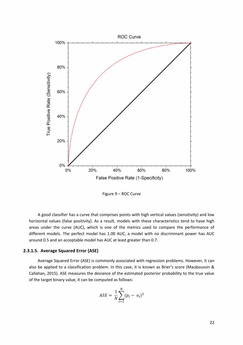
2.3.1.4. ROC Curve and AUC

The ROC curve is often used to examine the trade-off between the detection of true positives,

while avoiding the false positives. The characteristics of a typical ROC diagram are represented in

Figure 9. The proportion of true positives is shown on the vertical axis, while the proportion of false

positive can be seen on the horizontal axis.

22

Figure 9 – ROC Curve

A good classifier has a curve that comprises points with high vertical values (sensitivity) and low

horizontal values (false positivity). As a result, models with these characteristics tend to have high

areas under the curve (AUC), which is one of the metrics used to compare the performance of

different models. The perfect model has 1.00 AUC, a model with no discriminant power has AUC

around 0.5 and an acceptable model has AUC at least greater than 0.7.

2.3.1.5. Average Squared Error (ASE)

Average Squared Error (ASE) is commonly associated with regression problems. However, it can

also be applied to a classification problem. In this case, it is known as Brier’s score (Mauboussin &

Callahan, 2015). ASE measures the deviance of the estimated posterior probability to the true value

of the target binary value, it can be computed as follows:

𝐴𝑆𝐸 = 1

𝑁∑(𝑝𝑖 − 𝑜𝑖)2

𝑁

𝑖=1

23

N is the number of observations classified, 𝑝𝑖 is the estimated posterior probability of the 𝑖𝑡ℎ

observation and 𝑜𝑖 is its actual value. Small values for ASE indicate a high performance.

2.3.1.6. Cumulative Lift

The idea behind the cumulative lift is the assumption that a group of instances with high

estimated posterior probability should also be correlated with the actual success proportion (the

proportion of 1’s in a binary target data set). Therefore, if the observations are ranked according to

the posterior probabilities provided by a model, the group with the highest probability should also

have the highest success rate. Then, the success rate in this group has to be compared with the

success rate in the whole data set.

To compute the cumulative lift, a percentage that corresponds to the proportion of the data

that are going to be analyzed must first be defined. For example, if the proportion of the data to be

analyzed is 10% of a 100 instances data set, then the success proportion in the top 10 instances with

the highest probability is going to be compared to the success in the whole 100 instances in the data

set. The cumulative lift is computed as follows:

Cumulative Lift = 𝑆𝑢𝑐𝑐𝑒𝑠𝑠 𝑝𝑟𝑜𝑝𝑜𝑟𝑡𝑖𝑜𝑛 𝑖𝑛 𝑡ℎ𝑒 𝑡𝑜𝑝 𝑥% 𝑔𝑟𝑜𝑢𝑝 𝑤𝑖𝑡ℎ ℎ𝑖𝑔ℎ𝑒𝑠𝑡 𝑝𝑜𝑠𝑡𝑒𝑟𝑖𝑜𝑟 𝑝𝑟𝑜𝑏𝑎𝑏𝑖𝑙𝑖𝑡𝑦

𝑆𝑢𝑐𝑒𝑠𝑠 𝑝𝑟𝑜𝑝𝑜𝑟𝑡𝑖𝑜𝑛 𝑖𝑛 𝑡ℎ𝑒 𝑤ℎ𝑜𝑙𝑒 𝑑𝑎𝑡𝑎 𝑠𝑒𝑡

This metric is extremely useful when we wish to have a classifier that is able to rank instances

based on their posterior probability, not only if the posterior probability exceeds a specific threshold.

Figure 10 represents of a lift chart. Notice that when the whole data set is used, the cumulative lift is

1.

Figure 10 - Lift Chart

24

3. PART II

This part of the report is dedicated to detail the approach taken to build a propensity to buy

personal accident insurance model at Ocidental Seguros. The objective of the model is to identify the

clients that are likely to buy. These clients are called leads, which are going to be contacted through a

campaign by sales agents.

3.1. METHODOLOGY

As mentioned in the first section, the methodology followed was a combination of CRISP-DM

and SEMMA. This section is focused on the description of each step of the methodology and relating

it to the theory presented in Part I.

3.1.1. Business Understanding

The marketing department at Ocidental Seguros has several campaigns to advertise their

products and consequently increase its sales. By identifying clients that are likely to buy their

products (leads), we can gain understanding of the clients and save resources that would be spent on

valueless customers. That is the main reason why the company needs a predictive model designed to

predict propensity to buy.

Campaigns are evaluated according to several metrics. The three main metrics are:

1. Success Rate (Hit Rate): Success rate shows the general success of a campaign. It is simply

computed by the ratio between the number of sales divided by the number of contacts made

in a campaign.

𝑆𝑢𝑐𝑒𝑠𝑠 𝑟𝑎𝑡𝑒 =# 𝑆𝑎𝑙𝑒𝑠

# 𝐶𝑜𝑛𝑡𝑎𝑐𝑡𝑠

2. Simulation Rate: The simulation rate is the ratio between the number of simulations and

contacts made. This metric can also be interpreted as the effort that the sales agents put on

advertising the insurance products.

𝑆𝑖𝑚𝑢𝑙𝑎𝑡𝑖𝑜𝑛 𝑟𝑎𝑡𝑒 =# 𝑆𝑖𝑚𝑢𝑙𝑎𝑡𝑖𝑜𝑛𝑠

# 𝐶𝑜𝑛𝑡𝑎𝑐𝑡𝑠

3. Conversion Rate: Conversion rate is the ratio between the number of sales and the number of

simulation. As mentioned before, the simulations rate shows the effort of the commercial

team, if the commercial team is putting effort to increase simulations but the sales leads are

not appropriate, the conversion rate tends to be low. In comparison, if the leads are suitable to

the campaign and the sales agents work effectively, then the conversion rate tends to be high.

𝐶𝑜𝑛𝑣𝑒𝑟𝑠𝑖𝑜𝑛 𝑟𝑎𝑡𝑒 =# 𝑆𝑎𝑙𝑒𝑠

# 𝑆𝑖𝑚𝑢𝑙𝑎𝑡𝑖𝑜𝑛𝑠

25

Ultimately, the goal of a campaign is to increase the success rate. Having in consideration that

not all leads are going to be contacted, it is essential that the final model is able to identify a group of

leads who are likely to buy a personal accident insurance product.

3.1.2. Data Understanding

3.1.2.1. Data Sources

The data used for modelling came from different sources and had different nature. First type of

data collected was demographical data such as age, gender and marital status. Secondly, variables

concerning insurance variables such as indications of owned products, counts of policies in each line

of business and client’s segment classification were added to the data set. Finally, Millennium BCP

provided financial variables, although they were codified because of privacy matters, having access

to this data was a valuable resource.

All variables were aggregated into one single ABT (Analytical Base Table) at client level. The

whole list of variables can be found in Table 14 in the Appendix.

3.1.2.2. Target Definition

The target definition was a critical step because of its implications on type of observations

selected. More importantly, the target definition had to take into account the business objectives.

For the personal accident propensity to buy model, three options for the target variable were

designed:

1. Cross Sell: Cross Sell is a campaign that contact the leads and offers a discount on the product

proportional to the number of distinct lines of business owned. Clients with a diverse portfolio

are offered higher discounts.

Universe: All clients contacted through this campaign between 1st June 2016 and 1st June

2017.

Target: The success events are the clients that were contacted and bought only a personal

accidents product.

Rejection Reason: This target definition was rejected because the company needed a

model that targeted clients without offering any associated discount.

2. Simulations: The simulations target definition was based on the simulations of the clients not

associated with any campaign.

Universe: All clients that made a simulation between 1st June 2016 and 1st June 2017.

Target: Clients that made a simulation and converted (purchased a personal accident

policy).

Rejection Reason: Clients that make simulation already show interest in the product,

which was not the appropriate type of clients to be targeted.

26

3. Possessions: This target definition was based on the assumption that all active clients (client

that have at least one active policy) that never had personal accident before could have

purchased a product within the period of analysis.

Universe: All clients that were active between 1st June 2016 and 1st June 2017 and

had never had a personal accident product before.

Target: With this definition, the success events are the clients that purchased a personal

accident policy without any discount.

Rejection Reason: Not rejected.

Among the three possible options of the target variable, the option selected was the

Possessions target because it avoided the selection of clients already prone to buy, as it was the case

of the Simulations target. Furthermore, it also handled the effect of discounts by excluding the

clients that bought products discount. Then, the target variable was specified as follows:

1. Target variable: Binary variable that indicates if a client bought a Personal Accident product

without a discount between 1st June 2016 and 1st June 2017.

2. Data Universe:

1’s: All clients that have never had a Personal Accident product and purchased one without

a discount between 1st June 2016 and 1st June 2017.

0’s: All active clients between 1st June 2016 and 1st June 2017 who had never owned a

Personal Accidents product and did not purchased any Personal Accidents during the

period of analysis.

Once the target variable has been selected, the data concerning the instances in the target

variable was collected and the data preparation phase was reached. Additionally, the data set had

405886 observations of which 758 were success events. Therefore, the proportion of success was

0.18%.

3.1.3. Data Preparation

In this step the input data started to be analyzed. The first step is importing the data to SAS EM,

during this process the variable roles were defined (target, input, ID, etc.) and variables levels

(binary, interval, nominal, etc.). A preliminary exploration is done during this operation. For instance,

when creating the data source, only variables that had less than 20% of missing values and nominal

variables with less than 20 classes were selected, and were not unary. The variables rejected during

this phase are shown in Table 15 in the Appendix.

Initially, the number of variables in the data set was 392. After creating the data source in SAS

EM and applying the filtering criteria previously described, the total number of variables is 298, of

which 284 are inputs. In addition, some variables were excluded for conceptual reasons. For

example, the number of simulations in the last seven days was excluded because a sale is always

associated to a simulation. Then, one of the most important variables would be the number of

27

simulations in the past seven days. Hence, leads that are likely to buy in a longer term should also be

considered, but the variables associated with long term purchases would be disregarded by the

model.

The next step is to compute descriptive statistics to understand and gain acquaintance of the

data. More importantly, the analysis of the distribution of the variables is important at this stage. It is

visible that the age variable of the individuals in the data set has a bell shaped distribution (Figure

11). However, the majority of the variables in the dataset are highly positively skewed, particularly

the variables that are counts of events such as the number of claims, as shown in Figure 12.

Figure 11 – Distribution of Idade_Adj

28

Figure 12 – Distribution of No_Claims_Ever_NH

Based on the plots of the variables it is clear the presence of outliers in the data set. To diminish

the impact of outliers in the modelling phase, a truncation strategy was employed. That is, for

variables with values that exceeded a manual threshold defined by visual inspection, we replaced

them by a specified threshold value. This approach was taken because it avoided the exclusion of

more success event in the data set or introduce more bias by filtering only the non-event.

Another fundamental obstacle that had to be overcome was the presence of missing values in

some variables. For numeric variables, the median was assigned, since the vast majority of the

variables are highly skewed. In case of nominal/categorical variables, the approach adopted was to

assign the most frequent level.

One of the most important decisions to be made during this phase is the sampling strategy. The

proportion of success in the data set is almost negligible. To counter the imbalance in the data set, all

the success events were selected and a random sample of the non-event observations was drawn to

equally balance the data to a 50:50 proportion of events and non-events. Hence, the sample

obtained has 758 events and 758 non-events.

The consequences of equally balancing the data are reflected in the posterior probabilities

because the models assume that the proportion of events in the population is equal to the training

data, which is not true. The possible solutions for this problem are discussed in section 3.1.5.

After drawing a sample, it is good practice to compare the distributions and descriptive statistics

between the whole data set and the sample to verify that the sample is truly representative of the

population. As an example, comparing Figure 13 to Figure 11 the similarity in the distribution of

Idade_Adj can be observed, demonstrating that the sample is representative of the population. The

29

statistics comparison of the variable in the whole data set and the sample can be analyzed in Table

16 and Table 17 in the Appendix.

Figure 13 – Sample Distribution of Idade-Adj

The last process of this stage consisted of partitioning the sample into training and validation

sets. The sample could have been partitioned into training, validation and test data. However,

because of the small size of the sample, it was decided to partition the sample into training and

validation data to have more observations used to train the models. Yet, a test data set posteriorly

collected to assess the performance of the final model, section 3.1.5 describes this process. The

distribution of the sample was defined to be 70% training and 30% data. Table 3 displays the result of

the data partition.

Data Role Level 0 1 Totals

Train 530 531 1061

Validation 228 227 455

Totals 758 758 1516

Table 3 – Data Partition.

As previously stated, the data set has a large number of inputs, before modelling a variable

selection method must be determined to reduce dimensionality, especially if the modelling algorithm

has no built-in method of selecting important variables, such as artificial neural networks.

30

3.1.3.1. Variable Selection

Removing redundant and irrelevant variables from the training data set often improves

prediction performance. A quick verification of redundancy in the data set can be made by looking at

the correlation matrix. In Figure 14, a representation of the correlation matrix can be seen, the

values highlighted in green indicate correlation higher than 0.65, while values highlighted in red

indicate correlations lower than -0.65. The correlations between binary variables were also

considered with φ correlation coefficient being considered in this case. The correlation between

binary variables and numeric variables was computed as the point-biserial correlation. Lastly, the

correlations between numeric variables were calculated using Pearson’s correlation coefficient,

although this metric only measures the linear relationship between quantitative variables, it is still a

popular approach to identify associations between variables.

Figure 14 – Correlation Matrix

Two variable selection procedures were used:

R-square: The R-Square method can be used with a binary as well as with an interval-scaled

target. With this method, variable selection is performed in three steps:

31

1. In the first step, a correlation analysis between each input and the target variable is

performed. All input variables with a squared correlation above a specified threshold (the

default threshold is 0.005) are considered for the next step, all the other variables are

rejected.

2. All the variables selected in the previous step are evaluated sequentially thorough a

forward stepwise regression. At each successive step, an additional input variable is

chosen that provides the largest incremental increase in the model’s R-square. The

stepwise process terminates when no remaining input variables can meet the Stop R-

Square criterion (the default minimum R-Square improvement is 0.0005).

3. A final logistic regression analysis is performed using the predictive values that are output

from the forward stepwise selection as the independent input. Because there is only one

input, only two parameters are estimated (the intercept and the slope). All variables

associated with significant models through an F-test are selected.

Chi-Square: When this criterion is selected, the selection process does not have two distinct

steps, as in the case of the R-square criterion. Instead, a binary chi-square based tree is grown.

Interval variables are binned to compute the chi-statistic, the number of bins can be specified

(the default is 5). Only training data is used to grow the tree. As a result, the tree overfits the

training data, which is not a problem, since predictive performance is not the goal at this stage.

The inputs considered in the growth of the tree are passed on to the next node with the

assigned role of Input.

Each variable selection method gives a different input data set. Therefore, the approach

adopted applies the modelling phase to each of the two resulting data sets. Then, a verification of

redundant inputs was carried based on the correlation matrix. High correlations between numeric

variables were not found. Since both methods are based on improvement of fit sequentially, it was

expected not have much redundancy among the selected inputs. However, high values of correlation

between pairs of binary variables and numeric variables were found, especially when the binary

variable is a binned version of the numeric variable, these few occurrences were kept.

3.1.4. Modelling

The modelling phase is carried in a similar manner for all data sets. Four algorithms were

employed during this stage, logistic regression, decision trees, neural networks and ensemble

models. Various configurations of these algorithms were tested. The diagram below exemplifies this

process.

32

Figure 15 – Modelling Process.

3.1.4.1. Regression Models

Logistic regression is an appropriate regression model for a binary response variable because it

attempts to predict the probability of a success event of a binary target variable. The event of

interest in this case is the purchase of a personal accident policy.

Several model configurations were applied, the first set of models were created with the input

variables unaltered but with different variable model selection methods. The three possible

methods, backwards, forward and stepwise were tested. In addition to choosing a model selection

method, a selection criterion must be determined. The selection criterion designated was the

Average Squared Error.

The second set of models was created similarly to the first set, the only difference is the addition

of polynomial terms up to the second degree for numeric variables. By adding polynomial terms, the

complexity of the model increases resulting in less prediction bias, but also increases the possibility

of overfitting. Another consequence of adding polynomial terms is some loss in interpretability.

Another option to add flexibility to models is to consider interaction among the terms. SAS EM

allows the inclusion of two factor interactions. When including interaction terms, it is also important

to decide if keeping hierarchies is necessary, it implies that during the model selection phase two

factor interaction terms are included in the model only if both main effects have been already

included. A set of regression models were created considering interaction terms without hierarchies,

allowing interaction between terms even if the main effects are not included in the model.

Finally, the fourth and last set of models created for regression considers polynomial terms and

interaction terms. The model selections tested were forward and stepwise. Backward selection was

ModellingVariable Selection

Data Source

R-SquarePredictive

Models

Chi-SquarePredictive

Models

33

not considered in this set because since we are considering interaction and polynomial terms, the

number of inputs is large, resulting in an immense number of coefficients that are computationally

expensive to train and overly complex.

Figure 16 - Regression Models

Figure 16 illustrates the process described above. The regression model with the best

performance was achieved with forward model selection and polynomial terms. Figure 17 represents

the model selection method. The horizontal values indicate the iteration, while the vertical values

show the average squared error. As it is observed, the lowest average squared error for the

validation data is reached in the 18th iteration, which indicates that this model considers 18 inputs.

The coefficients estimates are presented in Table 4.

34

Figure 17 – Regression model Average Squared Error

Parameter Class Estimate Pr >

ChiSq

Intercept 127.768 0.5103

G_REP_Cod_Segmento_New 0 307.605 0.6916

G_REP_Cod_Segmento_New 1 -67.107 0.7292

G_REP_Cod_Segmento_New 2 -70.026 0.7180

G_REP_Cod_Segmento_New 3 -79.082 0.6834

G_REP_Profession_class 0 45.362 <.0001

G_REP_Profession_class 1 33.665 .

G_REP_Profession_class 2 33.711 <.0001

Ind_Sim_6Mth 0 -0.4561 0.0016

Ind_hasActive_NaoVida 0 0.9129 <.0001

Ind_hasActive_VR_VendaAtiva 0 -11.289 <.0001

Ind_hasActive_VendaAssoc 0 0.5422 <.0001

VAR_10 0 72.664 .

VAR_17 0 0.6481 <.0001

VAR_54 -0.1685 0.0005

No_VR_VendaAtiva_Ever*No_VendaAssoc_Active -0.8701 0.0214

No_VR_VendaAtiva_Ever*SUM_of_Ind_CAP -19.865 0.0111

SUM_of_Ind_CAP*VAR_42 0.1140 0.0013

SUM_of_Ind_CAP*VAR_54 -0.1165 0.0242

VAR_29*VAR_42 0.0402 <.0001

VAR_42*VAR_44 -0.0429 <.0001

VAR_44*VAR_45 0.0248 0.0056

VAR_44*Years_Client -0.00646 0.0222

VAR_44*Yrs_Since_Latest_Purchase -0.0149 0.0008

Table 4 – Regression Model Coefficients.

The sign of the parameter estimates indicates the direction of contribution to the target

variable. Parameters with positive values contribute to the success of the target variable considering

35

all the other variables static, while variables with negative estimated coefficients contribute to the

non-success of the target variable. It is important to notice that class variables with c levels originate

c-1 indicator variables, with c > 2. For example, the variable G_REP_Cod_Segmento_New has five

levels from 0 to 4. Then, four binary variables are created to indicate if an observation belongs to the

level indicated in column Class of Table 4. Level 4 is not shown because it is the reference level.

Accuracy Sensitivity Specificity AUC Lift 10% ASE

Train 0,829 0,823 0,836 0,918 1,998 0,115

Validation 0,796 0,784 0,807 0,892 2,004 0,133

Table 5 – Regression Model Evaluation

The performance of this model according to various metrics is shown in Table 5, the complete

list of metrics calculated in SAS EM is available in Table 18 in the Appendix. Moreover, the

performance of the selected regression model can also be visually evaluated in Figure 18 and Figure

19, which show the ROC curves and misclassification rates for training and validation data. Although

the selected regression model has the lowest validation ASE, it does not have the lowest

misclassification rate for the validation data, the reason for choosing the ASE over misclassification

rate is discussed in section 3.1.5.

Figure 18 – Regression ROC Curve

36

Figure 19 – Regression Misclassification Rate

3.1.4.2. Decision Trees

Similarly to the regression models, many configurations of decision trees were tested (Figure

20). The first difference in configuration concerns the splitting rule criterion. As mentioned in section

5.1, the two splitting rule analyzed were the Chi-square statistic (p-value) and entropy reduction.

Then, the parameters varied in the two approaches are discussed separately below.

1. Criterion Based on Statistical Hypothesis Test (CHAID)

Significance Level: The CHAID method of tree construction specifies a significance level of a

Chi-square test to stop the tree growth. The split must have an associated p-value that

provides a logworth (–log10(𝑝 − 𝑣𝑎𝑙𝑢𝑒)) greater than −log10(𝑠𝑖𝑔𝑛𝑖𝑓𝑖𝑐𝑎𝑛𝑐𝑒 𝑙𝑒𝑣𝑒𝑙).

Figure 20 – Decision Tree Models

37

Hence, increasing the value if the significance levels, less discriminating the branches are.

The default significance level is 0.2, which generates a threshold value of approximately 0.7.

Significance levels of 0.1, 0.2, 0.5 and 0.7 were tested, with the best results obtained with

significance level equal to 0.5;

Maximum Branch: The number of branches determines how many splits a node can

produce. Besides being the default value, the minimum number of branches is 2, resulting

in a binary tree. Increasing the number maximum branches to 3 and 5 has not caused any

improvement on performance.

Maximum Depth: This value specifies the maximum number generations of nodes that we

want to allow in a decision tree. The maximum depth can be set to integers between 1 and

50, the default number of generations for the Maximum Depth is 6.

Bonferroni Adjustment: Bonferroni adjustments accounts for multiple tests that might

occur in a node. Applying this penalization causes the splitting to be more conservative.

Better results were achieved with Bonferroni adjustment;

Minimum Categorical Size: The minimum categorical size specifies the minimum number of

training observations that a categorical value must have before the category can be used in

a split search. Increasing this value has not caused any improvement in performance.

Assessment: Average Square Error.

2. Criteria Based on Impurity (Entropy)

Significance Level: Significance level is not applicable in the case of entropy based trees,

since no statistical test is computed;

Maximum Branch: Allowing more branches did not improved performance. The default

configuration of 2 branches (binary tree) resulted in lower Average Squared Error. One of

the reasons for this outcome is the greedy nature of CART.

Maximum Depth: Trees grow until they meet the stopping criterion or the maximum depth

is reached. Then, allowing a tree to grow further it can increase performance, but it also

increases the chances of overfitting.

Bonferroni Adjustment: This option is not applicable for entropy based trees.

Minimum Categorical Size: Increasing the default value of 5 in the minimum categorical

size resulted in better performance.

Assessment: Average Square Error.

All the models were evaluated with ASE as a selection criterion, tress evaluated with this metric

are known as probability trees. The tree model with the lowest ASE on validation data was obtained

with entropy reduction set as splitting rule and configuration options shown in Table 6.

38

Decision Tree Configuration

Nominal Target Criterion: Entropy

Significance Level: -

Maximum Branch: 2

Maximum Depth: 10

Minimum Categorical Size:

10

Assessment: Average Square Error

Table 6 – Decision Tree Configuration

The performance of the model according to the metrics discussed in section 2.3 are analysed in Table 7.

Accuracy Sensitivity Specificity AUC Lift10% ASE

Train 0,823 0,772 0,874 0,901 1,998 0,124

Validation 0,800 0,727 0,873 0,868 1,917 0,145

Table 7 – Decision Tree Evaluation

Figure 21 illustrates the pruning phase and how the final tree was obtained by decreasing the

ASE on validation set while avoiding overfitting. Decreasing the ASE error also causes a reduction in

misclassification rate, as presented in Figure 22. Furthermore, the performance of the model can be

visualized through the ROC curve in both training and validation data in Figure 23, both plots show

large areas under the curve.

Figure 21 – Decision Tree Average Squared Error

39

Figure 22 – Decision Tree Misclassification Rate

Figure 23 – Decision Tree ROC curves.

40

In summary, the performance of the selected tree model is satisfactory. The interpretation of

the tree mode is easily made by looking at the tree structure in Figure 24. For visualization purposes,

only the top two levels are shown, the whole tree structure can be found in the appendix (Figure 35).

The root node uses the variable G_REP_Cod_Segmento_New to split the data into two branches, the

right branch indicates that the value of the class G_REP_Cod_Segmento_New variable is 0.

Additionally, belonging to this class has a positive contribution to be a success event because the

proportion of events, which is an estimation of the posterior probability, are higher than the

preceding node on both training and validation data. Moreover, since the proportion of event in this

node is 100% on training data, no further splitting is required and a leaf node is created, the

observations that fall into this node are classified as success events. The blue scale of the colour of

the nodes indicates the percentage of observations correctly classified in the training data.

Figure 24 – Decision Tree Structure

3.1.4.3. Artificial Neural Networks

Following the same strategy of building regression models and decision trees, different

configurations of neural networks were tested.

Two parameters were analyzed, the number of hidden units and the activation function. The

number of hidden units indicates the complexity of the models because only artificial neural

networks with one hidden layer were built. The activation function of a unit defines the output of

that unit given an input or set of inputs. Only two activation functions were considered, the sigmoid

function and 𝑡𝑎𝑛ℎ (hyperbolic tangent) function.

A key difference between neural networks and the models applied previously is the absence of a

variable selection mechanism. As a result, the model has to estimate a large number of parameters,

which can lead to overfitting. To counter this problem, the inputs selected in the regression and

41

decision tree models were used. This method reduced the number of inputs and led to better results.

Figure 25 shows the process adopted for building the artificial neural network model.

Figure 25 – Artificial Neural Networks Models

The first step of reducing the number of inputs based on the other models was crucial. Figure 26

illustrates the performance of the model using all the input variables available after the R-Square

variable selection with the standard SAS EM configurations (3 hidden units and 𝑡𝑎𝑛ℎ activation

function), it was clear that the model quickly overfits and its performance was poor compared to

other models built previously.

Figure 26 – Artificial Neural Network ASE with all inputs.

The lowest validation ASE was reached by configuring an artificial neural network with nine

hidden units and 𝑡𝑎𝑛ℎ set as the activation function. The inputs of the model variables were the

same variables used by the final regression model in section 3.1.4.1. Analyzing the performance

42

metrics in Table 8, it is evident that the model has a high performance and similarly to the other

models built, the specificity is higher than the sensitivity. Additionally, this model has the lowest ASE

among the artificial neural networks, decision trees and regression models.

Accuracy Sensitivity Specificity AUC Lift10% ASE

Train 0,824 0,804 0,843 0,921 1,998 0,114

Validation 0,809 0,793 0,825 0,897 2,004 0,129

Table 8 – Artificial Neural Network Evaluation

Figure 27 – Artificial Neural Network Average Squared Error.

Figure 28 – Artificial Neural Network Misclassification Rate.

43

Figure 29 – Artificial Neural Network ROC curves.

Based on Figure 27 and Figure 28 we can see how artificial neural networks can quickly overfit.

Moreover, Figure 29 shows how the performance is similar on training and validation data.

Despite having a decent performance, the lack of interpretability of artificial neural networks

may be a disadvantage in a business context, due to the impossibility of explaining to the

stakeholders the driving factors for purchasing a personal accident product.

3.1.4.4. Ensemble Models

The combination of several models usually produces better estimates. In SAS EM there are three

possible ways of combining the output of different input models:

Voting: This method is available for categorical targets only. When we use the voting method

to compute the posterior probabilities, the posterior probability is averaged among the models

that agree with the majority of the votes;

Maximum: The maximum posterior probability is taken among the set of input models;

Average: The average of the posteriori probabilities is taken regardless of the target event

level.

If all the input models provide the same posterior probability, there is no variability and the

ensemble model does not provide any enhancement in performance regardless of the function used

to combine them. In Figure 30, the top 250 posterior probabilities of the regression, decision tree

and artificial neural networks models combined in an ensemble model provide less extreme

posterior probabilities.

44

Figure 30 – Posterior Probabilities

The ensemble model with average combination function had the highest performance among

the available options. The performance metrics in Table 9 demonstrate the high performance of the

model, the same conclusion can be drawn looking at the ROC Curves in Figure 31. The lowest

validation ASE among all the models is achieved with this model. The complete list of metrics

computed in SAS EM is available in Table 18 in the Appendix.

Accuracy Sensitivity Specificity AUC Lift10% ASE

Train 0,853 0,812 0,894 0,935 1,998 0,105

Validation 0,822 0,775 0,868 0,907 2,004 0,124

Table 9 – Ensembel Model evaluation

45

Figure 31 – Ensemble Model ROC Curves

3.1.5. Final Evaluation and Results

The evaluation of the models must take into account the business aspects of how the campaigns

are implemented. For this reason, the evaluation of the models had two phases. The first phase is

related to the development of the models and how their parameters are configured to achieve a

good performance. During this phase, the choice of the models was mainly based on the average

squared error because the objective was to provide posterior probabilities close to the target value,

either 0 or 1. Then, the second phase determines the best model based on the lift of the model,

which means that the model that not only correctly classifies the instances, but also is able to rank

them based on the posterior probabilities. As a result, the lift is used as the final evaluation criterion

for model selection because only a portion of the clients are contacted for marketing campaigns,

which corresponds to the group with the highest posterior probability.

Figure 32 shows the performance comparison of the best models according to the cumulative

lift on the validation data. Except for the decision tree model, the other three models have the same

performance for lifts up to around 15% of depth. Nonetheless, as the depth increases the model with

the highest lift is the ensemble model. Also, comparing the metrics in Table 10 and Table 11, the

highest performance in the majority of the metrics is obtained with the ensemble model.

46

Figure 32 – Cummulative Lift Comparison

Ensemble

Artificial Neural

Network Regression

Decision Tree

Train: ASE 0,105 0,114 0,115 0,124

Train: Roc Index 0,935 0,921 0,918 0,901

Train: Accuracy 0,853 0,824 0,829 0,823

Train: Sensitivity 0,812 0,804 0,823 0,772

Train: Specificity 0,894 0,843 0,836 0,874

Train: AUC 0,935 0,921 0,918 0,901

Train: Lift 10% 1,998 1,998 1,998 1,998

Table 10 – Training Performance Comparison.

Ensemble Artificial Neural

Network Regression

Decision Tree

Validation: ASE 0,124 0,129 0,133 0,145

Validation: Roc Index 0,907 0,897 0,892 0,868

Validation: Accuracy 0,822 0,809 0,796 0,800

Validation: Sensitivity 0,775 0,793 0,784 0,727

Validation: Specificity 0,868 0,825 0,807 0,873

Validation: AUC 0,907 0,897 0,892 0,868

Validation: Lift 10% 2,004 2,004 2,004 1,917

Table 11 – Validation Performance Comparison.

3.1.5.1. Posterior Probability Adjustment

During the data preparation phase the sampling strategy defined included all the events of the

whole data set and a random sample of the non-events in the whole data set was taken to balance

the sample, this procedure is known as under-sampling the majority class. Then, the models were

trained and evaluated on this sample. However, the true proportion of events in the population is

not the proportion in the sample. As a result, the models do not reflect the actual circumstances.

To counter the problem of balancing the data, the posterior probabilities must be adjusted. A

possible way of performing the adjustment is presented below (Wielenga, 2017).

47

Assume:

𝑃 is the unadjusted predicted probability of the target event based on the model;

𝑃𝑎𝑑𝑗 is the adjusted predicted probability of the target event based on the model;

𝑝1 is the proportion of the target events in the sample;

𝑝0 = 1 − 𝑝1 is the proportion of non-events in the sample;

𝜏1 is the proportion of the target events in the population;

𝜏0 = 1 − 𝜏1 is the proportion of non-events in the population.

𝑃𝑎𝑑𝑗 =(𝑃 ∗ 𝜏1 ∗ 𝑝0)

[(𝑃 ∗ 𝜏1 ∗ 𝑝0) + ((1 − 𝑃) ∗ 𝜏0 ∗ 𝑝1)]

The adjusted probabilities keep the same order, but are rescaled. That is, if we rank the

observations in decreasing order of unadjusted posterior probability, observations with high rank of

unadjusted probability also have a high rank for adjusted posterior probability.

3.1.5.2. Test Data Evaluation

A test data set was collected to assess the performance of the model in a real contacted. As

referred to earlier in section 3.1.2, the period of analysis for the training data is from 1st June 2016

and 1st June 2017. The test data involves all the active clients between 1st June 2017 and 31st

September 2017 and were not used in the modelling phase. The success event in the test data is

defined in the same way as in the training data (section 3.1.2.2), except for the period in which the

observations bought the policies.

The test data was scored with the final model and the unadjusted posterior probabilities

obtained are shown in Figure 33, which can be compared with the adjusted probabilities in Figure 34.

The adjusted probabilities reflect the true propensity to buy, which in reality is low for the majority

of the population. Moreover, the difference in the median between the shown in Table 12 indicates

the shift in probabilities after the adjustment.

Mean Std Dev Minimum Maximum Median N

Unadjusted Probabilities 0,552 0,303 0,001 1 0,509 499393

Adjusted Probabilities 0,215 0,358 0 1 0,029 499393

Table 12 – Probabilities statistics.

48

Figure 33 – Histogram of Unadjusted Probabilities.

Figure 34 – Histogram of Adjusted Probabilities.

After adjusting the posterior probabilities, we can compute the cumulative lift on the test data.

Although the rank of the observation is unaltered, which results in no difference in the lift, having a

49

more realistic estimate of the probability was important for the application of the model in other

projects. The size of the data is large, so the depth of the cumulative lift can be small. The lift at 5% is

1.95, resulting in a propensity to buy almost double in the top 5% highest probability group

compared to a random client selection. Table 13 contains the lift at the specified depths.

Depth Cum. Lift

5% 1,954

10% 1,437

Table 13 – Test Data Cumulative Lift.

50

4. CONCLUSIONS AND DEPLOYMENT

This project demonstrated an approach to developing a predictive model. The first part detailed

the theoretical aspects along with some business specifications. Two main data mining processes

(CRISP-DM and SEMMA) were presented and related to a predictive model development to establish

guidelines for the practical part. Then, the algorithms applied during the practical phase and their

evaluation were reviewed based on the literature.

The practical section started with the business understanding: how campaigns are evaluated

and how the predictive model applied to the propensity to buy can add value to the marketing

campaigns. After gained the knowledge of the business and identified its requirements, the data

related topics were discussed.

The data understanding phase presented the data sources and the nature of the data used as

inputs for the model. An important decision was also made during this phase: the definition of the

target variable. Three target variable were considered and a detailed analysis was conducted to

identify the most suitable target variable. The last task of this phase was the aggregation of all input

variables into one ABT (Analytical Base Table).

Before proceeding to the modelling phase, data preparation techniques were applied to ensure

that data was in the proper format to serve as input for modelling. During this stage, a descriptive

analysis of the data was conducted with the aim of analyzing the distribution of the variables and

investigate the existence of irregularities such as missing values, outliers, and redundancy. The

approaches taken to handle these irregularities were described. On top of that, the sampling strategy

was decided and the variable selection methods were explained and applied.

Although data understanding and data preparation took a large portion of the process, the focus

of the project was on the predictive modelling techniques. Several configurations of logistic

regression models, decision trees, artificial neural networks, and ensemble models were created and

evaluated. The final model was selected based on various metrics and its performance on test data

was also analyzed, confirming that the model contributes to the improvement of campaigns’ success.

Another important aspect to consider is the validation of the model, not only from a statistical

perspective, but also from a business point of view. The driving factors leading to a higher propensity

to buy were discussed with the product manager at Ocidental Seguros. These factors also provided

possible business opportunities through the interpretation of the models.

In conclusion, this project was an excellent opportunity to apply the theory in a commercial

scenario. Although the deployment of the model was not made for a specific personal accident

product campaign it has been integrated into other projects such as customer Next Best Offer (NBO)

and Customer Lifetime Value (CLV): both projects require a probability estimate for personal accident

acquisition.

4.1. LIMITATIONS AND RECOMMENDATIONS FOR FUTURE WORKS

Some limitation were identified and listed below along with recommendations for future work:

51

1. One of the main limitations of the model was its broad purpose. As discussed in section

3.1.2.2, the target definition was the most general among the three options, which resulted

into a large portion of the customers to be taken into consideration. Alternatively, a model

could have been designed for a specific segment of clients or a specific campaign.

2. A more technical limitation concerns the sampling strategy. The sampling strategy adopted

was under-sampling the majority target level (the non-events) to have a balanced dataset.

Consequently, a great deal of information was lost by reducing the number of non-events in

the sample. Many approaches could have attenuated the loss of information, SMOTE

(Synthetic Minority Over-sampling Technique) is a possible approach that could have been

adopted if it was available in SAS EM.

3. SAS EM has many modelling techniques available. Because of time constraints and the number

of topics that could be explored in this project, the modelling phase was limited to focus on

decision trees, regression model, artificial neural networks and ensemble models. Other

modelling techniques could have been applied to generate better results.

52

APPENDIX

Name Type Label

Cod_Nif Character Número fiscal de contribuinte

Target_AP Numeric Target Variable

Date Date Reference Date

ID_NIF_Date Character

Ind_Tomador Character Indicador de tomador

Ind_Pagador Character Indicador de pagador

Ind_PessoaSegura Character Indicador de Pessoa Segura

Profession_class Character Profession class

SEGMENT_ID Character Segment

Dt_Nascimento Date Data de nascimento

Idade Numeric Idade

Idade_Adj Numeric Idade_Adj

Cod_Genero Character Sexo

Escalao_Etario Character Escalão Etário

Cod_EstadoCivil Character Estado civil

Ind_PrimTit_Num Numeric Ind_PrimTit_Num

Ind_SegTit_Num Numeric Ind_SegTit_Num

Ind_ClienteBCP_Num Numeric Ind_ClienteBCP_Num

Cod_Segmento_New Character Cod_Segmento_New

Cod_Macrosegmento_New Character Cod_Macrosegmento_New

Ind_Country_PRT Numeric Ind_Country_PRT

Ind_Nacionalidade_PRT Numeric Ind_Nacionalidade_PRT

Cod_Postal Character Código Postal

Cod_Postal_4Digit Character Cod_Postal_4Digit

Camp_Contact Numeric Camp_Contact

Camp_Contact_SalesCamp Numeric Camp_Contact_SalesCamp

Camp_Contact_SimFollow Numeric Camp_Contact_SimFollow

Camp_Succ Numeric Camp_Succ

Camp_Succ_SalesCamp Numeric Camp_Succ_SalesCamp

Camp_Succ_SimFollow Numeric Camp_Succ_SimFollow

Camp_Unsucc Numeric Camp_Unsucc

Camp_Unsucc_SalesCamp Numeric Camp_Unsucc_SalesCamp

Camp_Unsucc_SimFollow Numeric Camp_Unsucc_SimFollow

Camp_Unsucc_Price Numeric Camp_Unsucc_Price

Camp_Unsucc_Price_SalesCamp Numeric Camp_Unsucc_Price_SalesCamp

Camp_Unsucc_Price_SimFollow Numeric Camp_Unsucc_Price_SimFollow

Num_Claims_Ever Numeric

No_Claims_Ever_NH Numeric

No_Claims_Vida Numeric

No_Claims_Financials Numeric

No_Claims_NaoVida_NH Numeric

No_Claims_AP Numeric

No_Claims_AT Numeric

No_Claims_AU Numeric

No_Claims_DI Numeric

No_Claims_MR Numeric

No_Claims_RC Numeric

53

No_Claims_Other Numeric

No_Claims_PPP Numeric

No_Claims_VR Numeric

No_Claims_Ann Numeric

No_Claims_CAP Numeric

No_Claims_PPR Numeric

No_Claims_UL Numeric

No_Claim_1Yr_NH Numeric

No_Claim_1Yr_H Numeric

No_Claim_1Yr_NaoVida_NH Numeric

No_Claim_1Yr_Fins Numeric

No_Claim_6Mth_H Numeric

No_Claim_6Mth_NH Numeric

No_Claim_6Mth_NaoVida_NH Numeric

No_Claim_6Mth_VR Numeric

No_Claim_6Mth_Fins Numeric

No_Claim_1Yr_VR Numeric

No_Claims_MR_bad Numeric

No_Claims_MR_good Numeric

Val_Claims Numeric

Val_Claims_Vida Numeric

Val_Claims_Fins Numeric

Val_Claims_NaoVida Numeric

Val_Claims_VR Numeric

Val_Claims_1Yr Numeric

Val_Claims_6Mth Numeric

Val_Claims_1Yr_Fins Numeric

Val_Claims_1Yr_NaoVida Numeric

Val_Claims_1Yr_VR Numeric

Val_Claims_6Mth_Fins Numeric

Val_Claims_6Mth_NaoVida Numeric

Val_Claims_6Mth_VR Numeric

No_Claims_7days Numeric

Val_Claims_7days Numeric

SUM_of_Ind_Complaint_Under4Days Numeric

SUM_of_Ind_Complaint_Over17Days Numeric

SUM_of_Ind_Request_Under3Days Numeric

SUM_of_Ind_Request_Over7Days Numeric

SUM_of_Ind_Any_Contact_6Mths Numeric

SUM_of_Ind_Complaint_6Mths Numeric

SUM_of_Ind_Request_6Mths Numeric

SUM_of_Ind_CompFulfilled_6Mths Numeric

SUM_of_Ind_Comp_rejected_6Mths Numeric

SUM_of_Ind_Any_Contact Numeric

SUM_of_Ind_Complaint Numeric

SUM_of_Ind_Request Numeric

SUM_of_Ind_CompFulfilled Numeric

SUM_of_Ind_CompRejected Numeric

SUM_of_Ind_Complaint_1Yr Numeric

SUM_of_Ind_Request_1Yr Numeric

SUM_of_Ind_Request_7days Numeric

SUM_of_Ind_Complaint_7days Numeric

Years_Client Numeric Years_Client

54

Active_Tenure Numeric Active_Tenure

Years_First_Prod_Till_Date Numeric Years_First_Prod_Till_Date

Yrs_Since_Latest_Purchase Numeric Yrs_Since_Latest_Purchase

Ind_Inactive_Client Numeric Ind_Inactive_Client

Ind_Inactive_Client_1Yr Numeric

Ind_Inactive_Client_6Mth Numeric

No_Active_Policies Numeric

No_Ended_Policies Numeric

No_Ever_Policies Numeric

No_Annuled_Policies Numeric

No_Annulled_FaltaPagamento Numeric

No_Annulled_PedidoCliente Numeric

No_Annulled_IniciativaBanc Numeric

No_Annulled_Resgatada Numeric

No_Annulled_TransCongenere Numeric

SUM_of_Ind_Vida Numeric

SUM_of_Ind_Financials Numeric

SUM_of_Ind_NaoVida Numeric

SUM_of_Ind_AP Numeric

SUM_of_Ind_AT Numeric

SUM_of_Ind_AU Numeric

SUM_of_Ind_DI Numeric

SUM_of_Ind_MR Numeric

SUM_of_Ind_RC Numeric

SUM_of_Ind_Other Numeric

SUM_of_Ind_PPP Numeric

SUM_of_Ind_VR Numeric

SUM_of_Ind_Ann Numeric

SUM_of_Ind_CAP Numeric

SUM_of_Ind_PPR Numeric

SUM_of_Ind_UL Numeric

No_LOBs_Ever Numeric No_LOBs_Ever

No_ProductLines_Ever Numeric No_ProductLines_Ever

No_LOBs_Active Numeric No_LOBs_Active

No_ProductLines_Active Numeric No_ProductLines_Active

Ind_Monoproduto Numeric Ind_Monoproduto

Ind_MonoProductLine Numeric Ind_MonoProductLine

No_AP_Active Numeric No_AP_Active

No_AT_Active Numeric No_AT_Active

No_AU_Active Numeric No_AU_Active

No_DI_Active Numeric No_DI_Active

No_MR_Active Numeric No_MR_Active

No_RC_Active Numeric No_RC_Active

No_Other_Active Numeric No_Other_Active

No_PPP_Active Numeric No_PPP_Active

No_VR_Active Numeric No_VR_Active

No_Ann_Active Numeric No_Ann_Active

No_CAP_Active Numeric No_CAP_Active

No_PPR_Active Numeric No_PPR_Active

No_UL_Active Numeric No_UL_Active

No_PL_Vida_Active Numeric No_PL_Vida_Active

No_PL_Fins_Active Numeric No_PL_Fins_Active

No_PL_NaoVida_Active Numeric No_PL_NaoVida_Active

55

No_VendaAtiva_Ever Numeric No_VendaAtiva_Ever

No_VendaAssoc_Ever Numeric No_VendaAssoc_Ever

No_VendaAtiva_Active Numeric No_VendaAtiva_Active

No_VendaAssoc_Active Numeric No_VendaAssoc_Active

Sum_PremPaid Numeric Sum_PremPaid

Sum_PremPaid_Active Numeric Sum_PremPaid_Active

Sum_PremPaid_Inactive Numeric Sum_PremPaid_Inactive

Sum_PremPaid_VendaAtiva Numeric Sum_PremPaid_VendaAtiva

Sum_PremPaid_VendaAssoc Numeric Sum_PremPaid_VendaAssoc

Sum_PremPaid_PL_Vida Numeric Sum_PremPaid_PL_Vida

Sum_PremPaid_PL_Fins Numeric Sum_PremPaid_PL_Fins

Sum_PremPaid_PL_NaoVida Numeric Sum_PremPaid_PL_NaoVida

Sum_PremPaid_1Yr Numeric Sum_PremPaid_1Yr

Sum_PremPaid_1Yr_Active Numeric Sum_PremPaid_1Yr_Active

Sum_PremPaid_1Yr_Inactive Numeric Sum_PremPaid_1Yr_Inactive

Sum_PremPaid_1Yr_PL_Fins Numeric Sum_PremPaid_1Yr_PL_Fins

Sum_PremPaid_1Yr_PL_NaoVida Numeric Sum_PremPaid_1Yr_PL_NaoVida

Sum_PremPaid_1Yr_PL_Vida Numeric Sum_PremPaid_1Yr_PL_Vida

Sum_PremPaid_1Yr_VendaAssoc Numeric Sum_PremPaid_1Yr_VendaAssoc

Sum_PremPaid_1Yr_VendaAtiva Numeric Sum_PremPaid_1Yr_VendaAtiva

Sum_PremPaid_6Mth Numeric Sum_PremPaid_6Mth

Sum_PremPaid_6Mth_Active Numeric Sum_PremPaid_6Mth_Active

Sum_PremPaid_6Mth_Inactive Numeric Sum_PremPaid_6Mth_Inactive

Sum_PremPaid_6Mth_PL_Fins Numeric Sum_PremPaid_6Mth_PL_Fins

Sum_PremPaid_6Mth_PL_NaoVida Numeric Sum_PremPaid_6Mth_PL_NaoVida

Sum_PremPaid_6Mth_PL_Vida Numeric Sum_PremPaid_6Mth_PL_Vida

Sum_PremPaid_6Mth_VendaAssoc Numeric Sum_PremPaid_6Mth_VendaAssoc

Sum_PremPaid_6Mth_VendaAtiva Numeric Sum_PremPaid_6Mth_VendaAtiva

Sum_PremPaid_NonFins Numeric Sum_PremPaid_NonFins

Sum_PremPaid_NonFins_VendaAssoc Numeric Sum_PremPaid_NonFins_VendaAssoc

Sum_PremPaid_NonFins_VendaAtiva Numeric Sum_PremPaid_NonFins_VendaAtiva

Channel_Classification Character Channel_Classification

Bank_ClientType_Class Character Bank_ClientType_Class

Channel_Classification_Active Character Channel_Classification_Active

Bank_ClientType_Active Character Bank_ClientType_Active

No_1Yr_Issued Numeric No_1Yr_Issued

No_1Yr_Issued_StillActive Numeric No_1Yr_Issued_StillActive

No_1Yr_Issued_VendaAtiva Numeric No_1Yr_Issued_VendaAtiva

No_1Yr_Issued_VendaAssoc Numeric No_1Yr_Issued_VendaAssoc

No_1Yr_Issued_NaoVida Numeric No_1Yr_Issued_NaoVida

No_1Yr_Issued_Fins Numeric No_1Yr_Issued_Fins

No_1Yr_Issued_VR Numeric No_1Yr_Issued_VR

No_6Mth_Issued Numeric No_6Mth_Issued

No_6Mth_Issued_Fins Numeric No_6Mth_Issued_Fins

No_6Mth_Issued_NaoVida Numeric No_6Mth_Issued_NaoVida

No_6Mth_Issued_StillActive Numeric No_6Mth_Issued_StillActive

No_6Mth_Issued_VendaAssoc Numeric No_6Mth_Issued_VendaAssoc

No_6Mth_Issued_VendaAtiva Numeric No_6Mth_Issued_VendaAtiva

No_6Mth_Issued_VR Numeric No_6Mth_Issued_VR

No_1Yr_Annulled Numeric No_1Yr_Annulled

No_6Mth_Annulled Numeric No_6Mth_Annulled

Ind_had_Vida Numeric

Ind_had_Fins Numeric

56

Ind_had_NaoVida Numeric

Ind_had_AP Numeric

Ind_had_AT Numeric

Ind_had_AU Numeric

Ind_had_DI Numeric

Ind_had_MR Numeric

Ind_had_RC Numeric

Ind_had_Other Numeric

Ind_had_PPP Numeric

Ind_had_VR Numeric

Ind_had_Ann Numeric

Ind_had_CAP Numeric

Ind_had_PPR Numeric

Ind_had_UL Numeric

Ind_hasActive_AP Numeric

Ind_hasActive_AT Numeric

Ind_hasActive_AU Numeric

Ind_hasActive_DI Numeric

Ind_hasActive_MR Numeric

Ind_hasActive_RC Numeric

Ind_hasActive_Other Numeric

Ind_hasActive_PPP Numeric

Ind_hasActive_VR Numeric

Ind_hasActive_Ann Numeric

Ind_hasActive_CAP Numeric

Ind_hasActive_PPR Numeric

Ind_hasActive_UL Numeric

Ind_hasActive_Vida Numeric

Ind_hasActive_Fins Numeric

Ind_hasActive_NaoVida Numeric

No_1Yr_Annulled_AP Numeric No_1Yr_Annulled_AP

No_1Yr_Annulled_AT Numeric No_1Yr_Annulled_AT

No_1Yr_Annulled_AU Numeric No_1Yr_Annulled_AU

No_1Yr_Annulled_DI Numeric No_1Yr_Annulled_DI

No_1Yr_Annulled_MR Numeric No_1Yr_Annulled_MR

No_1Yr_Annulled_Other Numeric No_1Yr_Annulled_Other

No_1Yr_Annulled_VR Numeric No_1Yr_Annulled_VR

No_1Yr_Annulled_Fins Numeric No_1Yr_Annulled_Fins

No_1Yr_Annulled_RC Numeric No_1Yr_Annulled_RC

No_1Yr_Annulled_PPP Numeric No_1Yr_Annulled_PPP

No_6Mth_Annulled_AP Numeric No_6Mth_Annulled_AP

No_6Mth_Annulled_AT Numeric No_6Mth_Annulled_AT

No_6Mth_Annulled_AU Numeric No_6Mth_Annulled_AU

No_6Mth_Annulled_DI Numeric No_6Mth_Annulled_DI

No_6Mth_Annulled_Fins Numeric No_6Mth_Annulled_Fins

No_6Mth_Annulled_MR Numeric No_6Mth_Annulled_MR

No_6Mth_Annulled_Other Numeric No_6Mth_Annulled_Other

No_6Mth_Annulled_PPP Numeric No_6Mth_Annulled_PPP

No_6Mth_Annulled_RC Numeric No_6Mth_Annulled_RC

No_6Mth_Annulled_VR Numeric No_6Mth_Annulled_VR

No_LOBs_Ended Numeric No_LOBs_Ended

Sum_PremPaid_VendaAtiva_Active Numeric Sum_PremPaid_VendaAtiva_Active

Sum_PremPaid_VendaAssoc_Active Numeric Sum_PremPaid_VendaAssoc_Active

57

Sum_PremAnual Numeric Sum_PremAnual

Avg_PremAnual Numeric

Avg_PremAnual_Active Numeric Avg_PremAnual_Active

Ind_1Yr_Issued Numeric

Ind_1Yr_Issued_StillActive Numeric

Ind_1Yr_Issued_VendaAtiva Numeric

Ind_1Yr_Issued_VendaAssoc Numeric

Ind_1Yr_Issued_NaoVida Numeric

Ind_1Yr_Issued_Fins Numeric

Ind_1Yr_Issued_VR Numeric

Ind_6Mth_Issued Numeric

Ind_6Mth_Issued_Fins Numeric

Ind_6Mth_Issued_NaoVida Numeric

Ind_6Mth_Issued_StillActive Numeric

Ind_6Mth_Issued_VendaAssoc Numeric

Ind_6Mth_Issued_VendaAtiva Numeric

Ind_6Mth_Issued_VR Numeric

Ind_1Yr_Annulled Numeric

Ind_6Mth_Annulled Numeric

Ind_hasActive_VendaAtiva Numeric

Ind_hasActive_VendaAssoc Numeric

No_MR_VendaAtiva_Ever Numeric

No_MR_VendaAssoc_Ever Numeric

No_MR_VendaAssoc_Active Numeric

No_MR_VendaAtiva_Active Numeric

Ind_hasActive_MR_VendaAssoc Numeric

Ind_hasActive_MR_VendaAtiva Numeric

No_VR_VendaAtiva_Ever Numeric

No_VR_VendaAtiva_Active Numeric

No_VR_VendaAssoc_Ever Numeric

No_VR_VendaAssoc_Active Numeric

Ind_hasActive_VR_VendaAtiva Numeric

Ind_hasActive_VR_VendaAssoc Numeric

Ind_had_VendaAtiva Numeric

Ind_had_VendaAssoc Numeric

Ind_had_MR_VendaAtiva Numeric

Ind_had_MR_VendaAssoc Numeric

Ind_had_VR_VendaAtiva Numeric

Ind_had_VR_VendaAssoc Numeric

Ind_Ended_Pol_7days Numeric

Ind_Annulled_Pol_7days Numeric

Ind_Inactive_Cli_7days Numeric

Ind_First_Purchase_7days Numeric

Ind_Sim_Ever Numeric Ind_Sim_Ever

Ind_Sim_1Yr Numeric Ind_Sim_1Yr

Ind_Sim_6Mth Numeric Ind_Sim_6Mth

Ind_Conv_Ever Numeric Ind_Conv_Ever

Ind_Conv_1Yr Numeric Ind_Conv_1Yr

Ind_Conv_6Mth Numeric Ind_Conv_6Mth

Ind_Sim_NoConv_Ever Numeric Ind_Sim_NoConv_Ever

Ind_Sim_NoConv_1Yr Numeric Ind_Sim_NoConv_1Yr

Ind_Sim_NoConv_6Mth Numeric Ind_Sim_NoConv~_6Mth

No_Sim_1Yr Numeric No_Sim_1Yr

58

No_Conv_1Yr Numeric No_Conv_1Yr

Ind_Sim_AT_7days Numeric Ind_Sim_AT_7days

Ind_Sim_AU_7days Numeric Ind_Sim_AU_7days

Ind_Sim_DI_7days Numeric Ind_Sim_DI_7days

Ind_Sim_MR_7days Numeric Ind_Sim_MR_7days

Ind_Sim_PPP_7days Numeric Ind_Sim_PPP_7days

AVG_of_Ind_Prem_GreaterThanAvg Numeric

AVG_of_Ind_Prem_GreaterThanMedia Numeric

Ind_has_BankVars Numeric

DT_REF Numeric

VAR_2 Numeric

VAR_3 Numeric

VAR_4 Numeric

VAR_5 Numeric

VAR_6 Numeric

VAR_22 Numeric

VAR_23 Numeric

VAR_28 Numeric

VAR_29 Numeric

VAR_30 Numeric

VAR_31 Numeric

VAR_32 Numeric

VAR_33 Numeric

VAR_35 Numeric

VAR_36 Numeric

VAR_37 Numeric

VAR_38 Numeric

VAR_39 Numeric

VAR_40 Numeric

VAR_41 Numeric

VAR_42 Numeric

VAR_43 Numeric

VAR_44 Numeric

VAR_45 Numeric

VAR_46 Numeric

VAR_47 Numeric

VAR_48 Numeric

VAR_49 Numeric

VAR_50 Numeric

VAR_51 Numeric

VAR_52 Numeric

VAR_53 Numeric

VAR_54 Numeric

VAR_55 Numeric

VAR_56 Numeric

VAR_57 Numeric

VAR_25 Character

VAR_24 Character

VAR_26 Character

VAR_64 Character

VAR_65 Character

VAR_66 Character

VAR_67 Character

59

VAR_69 Character

VAR_34 Numeric

VAR_60 Numeric

VAR_61 Numeric

VAR_17 Numeric

VAR_7 Numeric

VAR_9 Numeric

VAR_13 Numeric

VAR_16 Numeric

VAR_10 Numeric

VAR_18 Numeric

VAR_21 Numeric

VAR_19 Numeric

VAR_12 Numeric

VAR_20 Numeric

VAR_14 Numeric

VAR_11 Numeric

VAR_15 Numeric

VAR_58 Numeric

VAR_62 Numeric

VAR_63 Numeric

VAR_68 Numeric

VAR_59 Numeric

VAR_70 Numeric

VAR_8 Numeric

Val_CapitalObjecto_N Numeric Capital do Objecto_N

Val_CapitalObjecto_Median Numeric Capital do Objecto_Median

Table 14 –List of Input Variables

NAME LEVEL

Bank_ClientType_Active NOMINAL

Bank_ClientType_Class NOMINAL

Channel_Classification NOMINAL

Channel_Classification_Active BINARY

Cod_Postal NOMINAL

Cod_Postal_4Digit NOMINAL

DT_REF INTERVAL

Date INTERVAL

Dt_Nascimento INTERVAL

Escalao_Etario NOMINAL

Idade INTERVAL

Ind_Annulled_Pol_7days BINARY

Ind_ClienteBCP_Num BINARY

Ind_Ended_Pol_7days BINARY

Ind_First_Purchase_7days UNARY

Ind_Inactive_Cli_7days UNARY

Ind_Inactive_Client UNARY

Ind_Inactive_Client_1Yr UNARY

Ind_Inactive_Client_6Mth UNARY

Ind_Pagador UNARY

60

Ind_PessoaSegura UNARY

Ind_PrimTit_Num BINARY

Ind_SegTit_Num UNARY

Ind_Sim_AT_7days UNARY

Ind_Sim_AU_7days UNARY

Ind_Sim_DI_7days UNARY

Ind_Sim_MR_7days UNARY

Ind_Sim_PPP_7days UNARY

Ind_Tomador UNARY

Ind_had_AP UNARY

Ind_had_AT BINARY

Ind_had_AU BINARY

Ind_had_Ann BINARY

Ind_had_CAP BINARY

Ind_had_DI BINARY

Ind_had_Fins BINARY

Ind_had_MR BINARY

Ind_had_MR_VendaAssoc BINARY

Ind_had_MR_VendaAtiva BINARY

Ind_had_NaoVida BINARY

Ind_had_Other BINARY

Ind_had_PPP BINARY

Ind_had_PPR BINARY

Ind_had_RC BINARY

Ind_had_UL BINARY

Ind_had_VR BINARY

Ind_had_VR_VendaAssoc BINARY

Ind_had_VR_VendaAtiva BINARY

Ind_had_VendaAssoc BINARY

Ind_had_VendaAtiva BINARY

Ind_had_Vida BINARY

Ind_hasActive_AP UNARY

Ind_has_BankVars UNARY

No_1Yr_Annulled_AP UNARY

No_6Mth_Annulled_AP UNARY

No_AP_Active UNARY

No_Claim_1Yr_Fins UNARY

No_Claim_1Yr_VR UNARY

No_Claim_6Mth_Fins UNARY

No_Claim_6Mth_VR UNARY

No_Claims_7days INTERVAL

No_Claims_AP UNARY

No_Claims_Ann UNARY

No_Claims_CAP UNARY

No_Claims_Financials UNARY

No_Claims_MR_bad INTERVAL

No_Claims_PPR UNARY

No_Claims_UL UNARY

No_Claims_VR UNARY

No_Claims_Vida UNARY

SUM_of_Ind_AP UNARY

SUM_of_Ind_Complaint_7days BINARY

SUM_of_Ind_Complaint_Under4Days INTERVAL

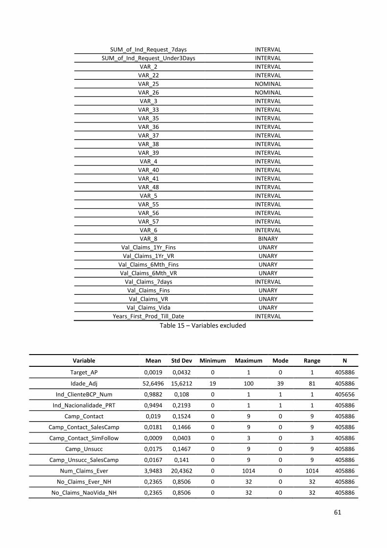
61

SUM_of_Ind_Request_7days INTERVAL

SUM_of_Ind_Request_Under3Days INTERVAL

VAR_2 INTERVAL

VAR_22 INTERVAL

VAR_25 NOMINAL

VAR_26 NOMINAL

VAR_3 INTERVAL

VAR_33 INTERVAL

VAR_35 INTERVAL

VAR_36 INTERVAL

VAR_37 INTERVAL

VAR_38 INTERVAL

VAR_39 INTERVAL

VAR_4 INTERVAL

VAR_40 INTERVAL

VAR_41 INTERVAL

VAR_48 INTERVAL

VAR_5 INTERVAL

VAR_55 INTERVAL

VAR_56 INTERVAL

VAR_57 INTERVAL

VAR_6 INTERVAL

VAR_8 BINARY

Val_Claims_1Yr_Fins UNARY

Val_Claims_1Yr_VR UNARY

Val_Claims_6Mth_Fins UNARY

Val_Claims_6Mth_VR UNARY

Val_Claims_7days INTERVAL

Val_Claims_Fins UNARY

Val_Claims_VR UNARY

Val_Claims_Vida UNARY

Years_First_Prod_Till_Date INTERVAL

Table 15 – Variables excluded

Variable Mean Std Dev Minimum Maximum Mode Range N

Target_AP 0,0019 0,0432 0 1 0 1 405886

Idade_Adj 52,6496 15,6212 19 100 39 81 405886

Ind_ClienteBCP_Num 0,9882 0,108 0 1 1 1 405656

Ind_Nacionalidade_PRT 0,9494 0,2193 0 1 1 1 405886

Camp_Contact 0,019 0,1524 0 9 0 9 405886

Camp_Contact_SalesCamp 0,0181 0,1466 0 9 0 9 405886

Camp_Contact_SimFollow 0,0009 0,0403 0 3 0 3 405886

Camp_Unsucc 0,0175 0,1467 0 9 0 9 405886

Camp_Unsucc_SalesCamp 0,0167 0,141 0 9 0 9 405886

Num_Claims_Ever 3,9483 20,4362 0 1014 0 1014 405886

No_Claims_Ever_NH 0,2365 0,8506 0 32 0 32 405886

No_Claims_NaoVida_NH 0,2365 0,8506 0 32 0 32 405886

62

No_Claims_AU 0,0897 0,5998 0 32 0 32 405886

No_Claims_DI 3,7118 20,3994 0 1012 0 1012 405886

No_Claims_MR 0,1281 0,542 0 25 0 25 405886

No_Claims_PPP 0,017 0,191 0 14 0 14 405886

No_Claim_1Yr_NH 0,0427 0,2897 0 12 0 12 405886

No_Claim_1Yr_H 0,4975 3,237 0 201 0 201 405886

No_Claim_1Yr_NaoVida_NH 0,0427 0,2897 0 12 0 12 405886

No_Claim_6Mth_H 0,2435 1,8028 0 112 0 112 405886

No_Claim_6Mth_NH 0,0247 0,2221 0 12 0 12 405886

No_Claim_6Mth_NaoVida_NH 0,0247 0,2221 0 12 0 12 405886

No_Claims_MR_bad 0,0596 0,3222 0 9 0 9 405886

No_Claims_MR_good 0,0686 0,3639 0 23 0 23 405886

Val_Claims 439,468 2453,98 0 311649,04 0 311649,04 405886

Val_Claims_NaoVida 439,468 2453,98 0 311649,04 0 311649,04 405886

Val_Claims_1Yr 56,464 849,792 0 223083,31 0 223083,31 405886

Val_Claims_6Mth 27,1801 692,283 0 223083,31 0 223083,31 405886

Val_Claims_1Yr_NaoVida 56,464 849,792 0 223083,31 0 223083,31 405886

Val_Claims_6Mth_NaoVida 27,1801 692,283 0 223083,31 0 223083,31 405886

Val_Claims_7days 0,0149 0,1506 0 9 0 9 405886

SUM_of_Ind_Request_Over7Days 0,2067 0,7038 0 47 0 47 405886

SUM_of_Ind_Any_Contact_6Mths 0,1436 0,6106 0 76 0 76 405886

SUM_of_Ind_Request_6Mths 0,1426 0,6075 0 76 0 76 405886

SUM_of_Ind_Any_Contact 1,2796 2,5454 0 177 0 177 405886

SUM_of_Ind_Complaint 0,0112 0,1333 0 12 0 12 405886

SUM_of_Ind_Request 1,2684 2,5243 0 177 0 177 405886

SUM_of_Ind_CompRejected 0,0071 0,1068 0 12 0 12 405886

SUM_of_Ind_Request_1Yr 0,2831 0,9125 0 83 0 83 405886

Years_Client 9,0897 5,6553 0,02 28,92 12,89 28,9 405886

Active_Tenure 7,6213 5,4548 0,0218 28,9194 12,887 28,8975 405886

Years_First_Prod_Till_Date 9,0897 5,6553 0,02 28,92 12,89 28,9 405886

Yrs_Since_Latest_Purchase 4,1214 3,9841 0,02 26,42 12,89 26,4 405886

No_Active_Policies 2,3321 2,2527 1 144 1 143 405886

No_Ended_Policies 1,3239 2,6438 0 173 0 173 405886

No_Ever_Policies 3,656 4,094 1 283 1 282 405886

No_Annuled_Policies 0,4878 1,0342 0 41 0 41 405886

No_Annulled_FaltaPagamento 0,1278 0,5093 0 16 0 16 405886

No_Annulled_PedidoCliente 0,1802 0,5269 0 18 0 18 405886

No_Annulled_Resgatada 0,1668 0,6082 0 41 0 41 405886

No_Annulled_TransCongenere 0,0095 0,1415 0 30 0 30 405886

SUM_of_Ind_Vida 2,323 3,8432 0 283 1 283 405886

SUM_of_Ind_Financials 1,7251 3,9172 0 283 0 283 405886

63

SUM_of_Ind_NaoVida 1,333 1,4621 0 42 1 42 405886

SUM_of_Ind_AT 0,0195 0,1633 0 8 0 8 405886

SUM_of_Ind_AU 0,2174 0,633 0 20 0 20 405886

SUM_of_Ind_DI 0,2089 0,5002 0 11 0 11 405886

SUM_of_Ind_MR 0,5823 0,8862 0 36 0 36 405886

SUM_of_Ind_RC 0,0126 0,1245 0 7 0 7 405886

SUM_of_Ind_PPP 0,2896 0,6808 0 12 0 12 405886

SUM_of_Ind_VR 0,5978 0,9483 0 17 0 17 405886

SUM_of_Ind_CAP 0,3307 0,791 0 22 0 22 405886

SUM_of_Ind_PPR 0,5851 1,0352 0 28 0 28 405886

SUM_of_Ind_UL 0,8092 3,3583 0 280 0 280 405886

No_LOBs_Ever 2,0867 1,0882 1 9 1 8 405886

No_ProductLines_Ever 1,5996 0,6432 1 3 1 2 405886

No_LOBs_Active 1,6372 0,8301 1 9 1 8 405886

No_ProductLines_Active 1,4283 0,5736 1 3 1 2 405886

Ind_Monoproduto 0,5413 0,4983 0 1 1 1 405886

Ind_MonoProductLine 0,6138 0,4869 0 1 1 1 405886

No_AT_Active 0,0131 0,1226 0 4 0 4 405886

No_AU_Active 0,1314 0,4023 0 11 0 11 405886

No_DI_Active 0,1312 0,3664 0 7 0 7 405886

No_MR_Active 0,4534 0,6773 0 20 0 20 405886

No_RC_Active 0,0098 0,1042 0 5 0 5 405886

No_PPP_Active 0,1325 0,3938 0 8 0 8 405886

No_VR_Active 0,4711 0,7608 0 13 0 13 405886

No_CAP_Active 0,165 0,4708 0 12 0 12 405886

No_PPR_Active 0,4225 0,8086 0 18 0 18 405886

No_UL_Active 0,4006 1,8709 0 143 0 143 405886

No_PL_Vida_Active 0,4711 0,7608 0 13 0 13 405886

No_PL_Fins_Active 0,9882 2,136 0 143 0 143 405886

No_PL_NaoVida_Active 0,8728 0,9325 0 23 1 23 405886

No_VendaAtiva_Ever 2,5882 4,0665 0 283 1 283 405886

No_VendaAssoc_Ever 1,0528 1,5588 0 24 0 24 405886

No_VendaAtiva_Active 1,5912 2,2234 0 144 1 144 405886

No_VendaAssoc_Active 0,7409 1,1492 0 14 0 14 405886

Sum_PremPaid 18770,9 74129,8 0 10630000 0 10630000 405886

Sum_PremPaid_Active 11966,8 44040,5 0 7930000 0 7930000 405886

Sum_PremPaid_Inactive 6811,36 43232,8 0 9100000 0 9100000 405886

Sum_PremPaid_VendaAtiva 17544 74263 0 10630000 0 10630000 405886

Sum_PremPaid_VendaAssoc 1226,86 3120,94 0 149177,32 0 149177,32 405886

Sum_PremPaid_PL_Vida 950,714 2769,38 0 147478,04 0 147478,04 405886

Sum_PremPaid_PL_Fins 16651,1 74099,4 0 10630000 0 10630000 405886

64

Sum_PremPaid_PL_NaoVida 1169,1 2997,41 0 116027,05 0 116027,05 405886

Sum_PremPaid_1Yr 1886,31 12888,9 0 2000010 0 2000010 405886

Sum_PremPaid_1Yr_Active 1874,81 12853,9 0 2000010 0 2000010 405886

Sum_PremPaid_1Yr_Inactive 12,4508 536 0 200000 0 200000 405886

Sum_PremPaid_1Yr_PL_Fins 1574,92 12888,6 0 2000010 0 2000010 405886

Sum_PremPaid_1Yr_PL_NaoVida 182,823 403,66 0 46326,18 0 46326,18 405886

Sum_PremPaid_1Yr_PL_Vida 128,57 375,663 0 22201,12 0 22201,12 405886

Sum_PremPaid_1Yr_VendaAssoc 159,465 424,833 0 23964,99 0 23964,99 405886

Sum_PremPaid_1Yr_VendaAtiva 1726,85 12898,3 0 2000010 0 2000010 405886

Sum_PremPaid_6Mth 751,428 8052,56 0 971158,76 0 971158,76 405886

Sum_PremPaid_6Mth_Active 749,106 8020,66 0 971158,76 0 971158,76 405886

Sum_PremPaid_6Mth_Inactive 2,6863 332,954 0 200000 0 200000 405886

Sum_PremPaid_6Mth_PL_Fins 592,02 8047,66 0 970000 0 970000 405886

Sum_PremPaid_6Mth_PL_NaoVida 93,3308 225,329 0 23620,94 0 23620,94 405886

Sum_PremPaid_6Mth_PL_Vida 66,0774 209,605 0 11879,73 0 11879,73 405886

Sum_PremPaid_6Mth_VendaAssoc 80,84 237,49 0 12428,76 0 12428,76 405886

Sum_PremPaid_6Mth_VendaAtiva 670,588 8053,82 0 971158,76 0 971158,76 405886

Sum_PremPaid_NonFins 2119,81 4353,03 0 160634,45 0 160634,45 405886

Sum_PremPaid_NonFins_VendaAssoc 1226,86 3120,94 0 149177,32 0 149177,32 405886

Sum_PremPaid_NonFins_VendaAtiva 892,944 2976,17 0 160634,45 0 160634,45 405886

No_1Yr_Issued 0,3572 0,8209 0 60 0 60 405886

No_1Yr_Issued_StillActive 0,3436 0,7917 0 60 0 60 405886

No_1Yr_Issued_VendaAtiva 0,2343 0,6525 0 60 0 60 405886

No_1Yr_Issued_VendaAssoc 0,1229 0,473 0 12 0 12 405886

No_1Yr_Issued_NaoVida 0,1754 0,4798 0 14 0 14 405886

No_1Yr_Issued_Fins 0,0959 0,501 0 60 0 60 405886

No_1Yr_Issued_VR 0,0859 0,3171 0 6 0 6 405886

No_6Mth_Issued 0,1787 0,6002 0 60 0 60 405886

No_6Mth_Issued_Fins 0,0486 0,3875 0 60 0 60 405886

No_6Mth_Issued_NaoVida 0,0897 0,3393 0 12 0 12 405886

No_6Mth_Issued_StillActive 0,1748 0,5897 0 60 0 60 405886

No_6Mth_Issued_VendaAssoc 0,0588 0,3231 0 12 0 12 405886

No_6Mth_Issued_VendaAtiva 0,1199 0,4873 0 60 0 60 405886

No_6Mth_Issued_VR 0,0405 0,2121 0 6 0 6 405886

No_1Yr_Annulled 0,0578 0,2901 0 13 0 13 405886

Ind_hasActive_AT 0,0122 0,1097 0 1 0 1 405886

Ind_hasActive_AU 0,1115 0,3147 0 1 0 1 405886

Ind_hasActive_DI 0,1225 0,3279 0 1 0 1 405886

Ind_hasActive_MR 0,3681 0,4823 0 1 0 1 405886

Ind_hasActive_RC 0,0093 0,0958 0 1 0 1 405886

Ind_hasActive_PPP 0,1152 0,3193 0 1 0 1 405886

65

Ind_hasActive_VR 0,3381 0,4731 0 1 0 1 405886

Ind_hasActive_CAP 0,1349 0,3416 0 1 0 1 405886

Ind_hasActive_PPR 0,3029 0,4595 0 1 0 1 405886

Ind_hasActive_UL 0,1212 0,3263 0 1 0 1 405886

Ind_hasActive_Vida 0,3381 0,4731 0 1 0 1 405886

Ind_hasActive_Fins 0,4782 0,4995 0 1 0 1 405886

Ind_hasActive_NaoVida 0,6119 0,4873 0 1 1 1 405886

No_1Yr_Annulled_AU 0,0115 0,1165 0 7 0 7 405886

No_1Yr_Annulled_DI 0,0088 0,0988 0 5 0 5 405886

No_1Yr_Annulled_MR 0,0102 0,1148 0 8 0 8 405886

No_1Yr_Annulled_VR 0,0108 0,1265 0 6 0 6 405886

No_1Yr_Annulled_Fins 0,0116 0,1361 0 10 0 10 405886

No_1Yr_Annulled_PPP 0,0033 0,0597 0 3 0 3 405886

No_6Mth_Annulled_AU 0,0057 0,0795 0 3 0 3 405886

No_6Mth_Annulled_DI 0,0045 0,0693 0 5 0 5 405886

No_6Mth_Annulled_Fins 0,0064 0,1009 0 10 0 10 405886

No_6Mth_Annulled_MR 0,0056 0,0832 0 6 0 6 405886

No_6Mth_Annulled_PPP 0,0017 0,0421 0 2 0 2 405886

No_LOBs_Ended 0,7913 0,9804 0 8 0 8 405886

Sum_PremPaid_VendaAtiva_Active 10944,5 44140,5 0 7930000 0 7930000 405886

Sum_PremPaid_VendaAssoc_Active 1022,32 2785,07 0 149177,32 0 149177,32 405886

Sum_PremAnual 21631,2 99728,3 -2709,34 19734693,9 0 19737403,2 405886

Avg_PremAnual 4313,48 12167,4 -2709,34 2280000 0 2282709,34 405886

Avg_PremAnual_Active 4232,8 13220,1 -2709,34 2280000 0 2282709,34 405886

Ind_1Yr_Issued 0,2331 0,4228 0 1 0 1 405886

Ind_1Yr_Issued_StillActive 0,2297 0,4206 0 1 0 1 405886

Ind_1Yr_Issued_VendaAtiva 0,1777 0,3823 0 1 0 1 405886

Ind_1Yr_Issued_VendaAssoc 0,0764 0,2657 0 1 0 1 405886

Ind_1Yr_Issued_NaoVida 0,1426 0,3497 0 1 0 1 405886

Ind_1Yr_Issued_Fins 0,0672 0,2503 0 1 0 1 405886

Ind_1Yr_Issued_VR 0,0762 0,2652 0 1 0 1 405886

Ind_6Mth_Issued 0,1227 0,3281 0 1 0 1 405886

Ind_6Mth_Issued_Fins 0,033 0,1785 0 1 0 1 405886

Ind_6Mth_Issued_NaoVida 0,0763 0,2655 0 1 0 1 405886

Ind_6Mth_Issued_StillActive 0,1213 0,3265 0 1 0 1 405886

Ind_6Mth_Issued_VendaAssoc 0,0378 0,1907 0 1 0 1 405886

Ind_6Mth_Issued_VendaAtiva 0,0941 0,2919 0 1 0 1 405886

Ind_6Mth_Issued_VR 0,0376 0,1903 0 1 0 1 405886

Ind_1Yr_Annulled 0,0473 0,2124 0 1 0 1 405886

Ind_hasActive_VendaAtiva 0,8084 0,3935 0 1 1 1 405886

Ind_hasActive_VendaAssoc 0,3658 0,4817 0 1 0 1 405886

66

No_MR_VendaAtiva_Ever 0,2993 0,6634 0 31 0 31 405886

No_MR_VendaAssoc_Ever 0,2829 0,5234 0 14 0 14 405886

No_MR_VendaAssoc_Active 0,2077 0,4273 0 12 0 12 405886

No_MR_VendaAtiva_Active 0,2457 0,5422 0 19 0 19 405886

Ind_hasActive_MR_VendaAssoc 0,1995 0,3996 0 1 0 1 405886

Ind_hasActive_MR_VendaAtiva 0,206 0,4044 0 1 0 1 405886

No_VR_VendaAtiva_Ever 0,0438 0,2168 0 6 0 6 405886

No_VR_VendaAtiva_Active 0,0355 0,1925 0 6 0 6 405886

No_VR_VendaAssoc_Ever 0,5541 0,9052 0 17 0 17 405886

No_VR_VendaAssoc_Active 0,4355 0,7248 0 13 0 13 405886

Ind_hasActive_VR_VendaAtiva 0,0342 0,1819 0 1 0 1 405886

Ind_hasActive_VR_VendaAssoc 0,3208 0,4668 0 1 0 1 405886

Ind_Sim_Ever 0,5378 0,4986 0 1 1 1 405886

Ind_Sim_1Yr 0,2396 0,4268 0 1 0 1 405886

Ind_Sim_6Mth 0,1332 0,3398 0 1 0 1 405886

Ind_Conv_Ever 0,3654 0,4815 0 1 0 1 405886

Ind_Conv_1Yr 0,1314 0,3378 0 1 0 1 405886

Ind_Conv_6Mth 0,0682 0,252 0 1 0 1 405886

Ind_Sim_NoConv_Ever 0,1724 0,3777 0 1 0 1 405886

Ind_Sim_NoConv_1Yr 0,1082 0,3106 0 1 0 1 405886

No_Sim_1Yr 0,4138 0,9221 0 18 0 18 405886

No_Conv_1Yr 0,1619 0,4625 0 12 0 12 405886

AVG_of_Ind_Prem_GreaterThanAvg 0,337 0,3537 0 1 0 1 336693

AVG_of_Ind_Prem_GreaterThanMedia 0,4795 0,3672 0 1 0 1 336693

VAR_23 5,3593 2,5829 0 9 5 9 329389

VAR_28 2,6982 2,7053 0 9 0 9 405886

VAR_29 1,8213 2,241 0 9 0 9 405886

VAR_30 2,6863 2,7613 0 9 0 9 405886

VAR_31 2,7975 3,0215 0 9 0 9 405886

VAR_32 2,4388 2,5558 0 9 0 9 405886

VAR_42 4,4449 2,9376 0 9 5 9 396217

VAR_43 3,0114 2,7748 0 9 0 9 396217

VAR_44 6,3703 2,6259 0 9 9 9 405886

VAR_45 2,7469 2,7398 0 9 0 9 405886

VAR_46 2,9259 2,3268 0 9 2 9 405886

VAR_47 2,6683 2,7796 0 9 0 9 405886

VAR_49 2,8605 3,0552 0 9 0 9 405886

VAR_50 2,6032 2,784 0 9 0 9 405886

VAR_51 2,6316 2,6734 0 9 0 9 405886

VAR_52 2,7843 2,7672 0 9 0 9 405886

VAR_53 2,8632 2,9633 0 9 0 9 405886

67

VAR_54 2,6332 2,7138 0 9 0 9 405886

VAR_34 4,8198 4,5268 2 91 4 89 392126

VAR_60 0,087 0,2818 0 1 0 1 405886

VAR_61 0,3342 0,4717 0 1 0 1 405886

VAR_17 0,7095 0,454 0 1 1 1 405886

VAR_7 0,6158 0,4864 0 1 1 1 405886

VAR_9 0,6459 0,4782 0 1 1 1 405886

VAR_13 0,6109 0,4875 0 1 1 1 405886

VAR_16 0,8897 0,3132 0 1 1 1 405886

VAR_10 0,9997 0,0163 0 1 1 1 405886

VAR_18 0,8117 0,3909 0 1 1 1 405886

VAR_21 0,4393 0,4963 0 1 0 1 405886

VAR_19 0,8078 0,3941 0 1 1 1 405886

VAR_12 0,6341 0,4817 0 1 1 1 405886

VAR_20 0,7043 0,4564 0 1 1 1 405886

VAR_14 0,5075 0,4999 0 1 1 1 405886

VAR_11 0,6777 0,4674 0 1 1 1 405886

VAR_15 0,7043 0,4564 0 1 1 1 405886

VAR_58 0,7939 0,4045 0 1 1 1 405886

VAR_62 0,9472 0,2236 0 1 1 1 405886

VAR_63 0,639 0,4803 0 1 1 1 405886

VAR_70 0,2952 0,4561 0 1 0 1 405886

VAR_8 0,5252 0,4994 0 1 1 1 405886

Val_CapitalObjecto_N 18,6797 30,4055 1 516 2 515 369873

Val_CapitalObjecto_Median 65048,1 39231,8 498,8 3018500 30000 3018001,2 369873

Ind_Sim_NoConv_6Mth 0,0651 0,2467 0 1 0 1 405886

Table 16 – Data set quantitative var. descriptive statistics.

Variable Mean Std Dev Minimum Maximum Range N

Target_AP 0,500 0,500 0 1 1 1516

Idade_Adj 53,088 16,321 19 96 77 1516

Ind_ClienteBCP_Num 0,979 0,144 0 1 1 1506

Ind_Nacionalidade_PRT 0,941 0,235 0 1 1 1516

Camp_Contact 0,036 0,213 0 3 3 1516

Camp_Contact_SalesCamp 0,028 0,185 0 2 2 1516

Camp_Contact_SimFollow 0,008 0,096 0 2 2 1516

Camp_Unsucc 0,034 0,208 0 3 3 1516

Camp_Unsucc_SalesCamp 0,026 0,180 0 2 2 1516

Num_Claims_Ever 2,946 17,514 0 337 337 1516

No_Claims_Ever_NH 0,168 0,734 0 16 16 1516

68

No_Claims_NaoVida_NH 0,168 0,734 0 16 16 1516

No_Claims_AU 0,060 0,574 0 16 16 1516

No_Claims_DI 2,778 17,443 0 337 337 1516

No_Claims_MR 0,084 0,402 0 4 4 1516

No_Claims_PPP 0,021 0,226 0 4 4 1516

No_Claim_1Yr_NH 0,030 0,225 0 5 5 1516

No_Claim_1Yr_H 0,390 3,354 0 86 86 1516

No_Claim_1Yr_NaoVida_NH 0,030 0,225 0 5 5 1516

No_Claim_6Mth_H 0,172 2,012 0 69 69 1516

No_Claim_6Mth_NH 0,019 0,196 0 5 5 1516

No_Claim_6Mth_NaoVida_NH 0,019 0,196 0 5 5 1516

No_Claims_MR_bad 0,047 0,281 0 4 4 1516

No_Claims_MR_good 0,038 0,239 0 4 4 1516

Val_Claims 328,105 1931,460 0 47160,69 47160,69 1516

Val_Claims_NaoVida 328,105 1931,460 0 47160,69 47160,69 1516

Val_Claims_1Yr 39,960 685,787 0 25500 25500 1516

Val_Claims_6Mth 27,480 667,011 0 25500 25500 1516

Val_Claims_1Yr_NaoVida 39,960 685,787 0 25500 25500 1516

Val_Claims_6Mth_NaoVida 27,480 667,011 0 25500 25500 1516

Val_Claims_7days 0,007 0,092 0 2 2 1516

SUM_of_Ind_Request_Over7Days 0,178 0,652 0 10 10 1516

SUM_of_Ind_Any_Contact_6Mths 0,116 0,451 0 5 5 1516

SUM_of_Ind_Request_6Mths 0,115 0,442 0 5 5 1516

SUM_of_Ind_Any_Contact 1,216 2,546 0 34 34 1516

SUM_of_Ind_Complaint 0,007 0,106 0 2 2 1516

SUM_of_Ind_Request 1,209 2,531 0 34 34 1516

SUM_of_Ind_CompRejected 0,007 0,096 0 2 2 1516

SUM_of_Ind_Request_1Yr 0,238 0,785 0 12 12 1516

Years_Client 8,249 5,738 0,02 27,32 27,3 1516

Active_Tenure 6,838 5,419 0,021858 24,552287 24,530429 1516

Years_First_Prod_Till_Date 8,249 5,738 0,02 27,32 27,3 1516

Yrs_Since_Latest_Purchase 3,846 3,930 0,02 20,42 20,4 1516

No_Active_Policies 2,210 2,428 1 37 36 1516

No_Ended_Policies 1,370 3,266 0 70 70 1516

No_Ever_Policies 3,580 4,811 1 81 80 1516

No_Annuled_Policies 0,475 1,017 0 10 10 1516

No_Annulled_FaltaPagamento 0,110 0,457 0 6 6 1516

No_Annulled_PedidoCliente 0,165 0,533 0 5 5 1516

No_Annulled_Resgatada 0,187 0,621 0 8 8 1516

No_Annulled_TransCongenere 0,011 0,128 0 3 3 1516

SUM_of_Ind_Vida 2,527 4,583 0 80 80 1516

69

SUM_of_Ind_Financials 1,922 4,640 0 80 80 1516

SUM_of_Ind_NaoVida 1,053 1,439 0 13 13 1516

SUM_of_Ind_AT 0,023 0,218 0 6 6 1516

SUM_of_Ind_AU 0,151 0,554 0 6 6 1516

SUM_of_Ind_DI 0,193 0,490 0 5 5 1516

SUM_of_Ind_MR 0,376 0,770 0 8 8 1516

SUM_of_Ind_RC 0,011 0,111 0 2 2 1516

SUM_of_Ind_PPP 0,298 0,719 0 7 7 1516

SUM_of_Ind_VR 0,605 0,922 0 8 8 1516

SUM_of_Ind_CAP 0,340 0,763 0 8 8 1516

SUM_of_Ind_PPR 0,639 1,276 0 28 28 1516

SUM_of_Ind_UL 0,943 3,808 0 75 75 1516

No_LOBs_Ever 1,962 1,061 1 8 7 1516

No_ProductLines_Ever 1,517 0,636 1 3 2 1516

No_LOBs_Active 1,509 0,775 1 5 4 1516

No_ProductLines_Active 1,319 0,521 1 3 2 1516

Ind_Monoproduto 0,629 0,483 0 1 1 1516

Ind_MonoProductLine 0,708 0,455 0 1 1 1516

No_AT_Active 0,014 0,151 0 4 4 1516

No_AU_Active 0,083 0,344 0 4 4 1516

No_DI_Active 0,110 0,328 0 2 2 1516

No_MR_Active 0,270 0,582 0 6 6 1516

No_RC_Active 0,009 0,102 0 2 2 1516

No_PPP_Active 0,137 0,399 0 4 4 1516

No_VR_Active 0,473 0,714 0 4 4 1516

No_CAP_Active 0,183 0,471 0 4 4 1516

No_PPR_Active 0,435 0,801 0 7 7 1516

No_UL_Active 0,495 2,083 0 36 36 1516

No_PL_Vida_Active 0,473 0,714 0 4 4 1516

No_PL_Fins_Active 1,114 2,363 0 36 36 1516

No_PL_NaoVida_Active 0,623 0,894 0 10 10 1516

No_VendaAtiva_Ever 2,702 4,779 0 81 81 1516

No_VendaAssoc_Ever 0,869 1,455 0 13 13 1516

No_VendaAtiva_Active 1,645 2,434 0 36 36 1516

No_VendaAssoc_Active 0,565 0,977 0 6 6 1516

Sum_PremPaid 22136,750 92325,190 0 1899035,8 1899035,8 1516

Sum_PremPaid_Active 13617,800 44435,050 0 737193,68 737193,68 1516

Sum_PremPaid_Inactive 8540,150 66299,890 0 1662500 1662500 1516

Sum_PremPaid_VendaAtiva 21173,270 92403,150 0 1899035,8 1899035,8 1516

Sum_PremPaid_VendaAssoc 963,484 3097,300 0 41699 41699 1516

Sum_PremPaid_PL_Vida 862,112 2866,890 0 40232,16 40232,16 1516

70

Sum_PremPaid_PL_Fins 20405,810 91886,920 0 1862500 1862500 1516

Sum_PremPaid_PL_NaoVida 868,832 2896,380 0 44063,06 44063,06 1516

Sum_PremPaid_1Yr 2740,240 14841,960 0 305010 305010 1516

Sum_PremPaid_1Yr_Active 2733,260 14839,040 0 305010 305010 1516

Sum_PremPaid_1Yr_Inactive 8,181 60,930 0 1072,85 1072,85 1516

Sum_PremPaid_1Yr_PL_Fins 2476,550 14853,350 0 305010 305010 1516

Sum_PremPaid_1Yr_PL_NaoVida 132,157 355,011 0 3983,12 3983,12 1516

Sum_PremPaid_1Yr_PL_Vida 131,534 415,000 0 5298,82 5298,82 1516

Sum_PremPaid_1Yr_VendaAssoc 133,837 432,117 0 5477,92 5477,92 1516

Sum_PremPaid_1Yr_VendaAtiva 2606,400 14855,670 0 305010 305010 1516

Sum_PremPaid_6Mth 1465,010 11506,770 0 305010 305010 1516

Sum_PremPaid_6Mth_Active 1463,540 11506,850 0 305010 305010 1516

Sum_PremPaid_6Mth_Inactive 1,860 22,485 0 537,17 537,17 1516

Sum_PremPaid_6Mth_PL_Fins 1329,010 11513,800 0 305010 305010 1516

Sum_PremPaid_6Mth_PL_NaoVida 65,181 182,306 0 2225,38 2225,38 1516

Sum_PremPaid_6Mth_PL_Vida 70,813 250,220 0 3810,79 3810,79 1516

Sum_PremPaid_6Mth_VendaAssoc 70,727 264,319 0 3810,79 3810,79 1516

Sum_PremPaid_6Mth_VendaAtiva 1394,280 11511,450 0 305010 305010 1516

Sum_PremPaid_NonFins 1730,940 4454,410 0 55421,27 55421,27 1516

Sum_PremPaid_NonFins_VendaAssoc 963,484 3097,300 0 41699 41699 1516

Sum_PremPaid_NonFins_VendaAtiva 767,460 2872,110 0 44063,06 44063,06 1516

No_1Yr_Issued 0,422 0,880 0 8 8 1516

No_1Yr_Issued_StillActive 0,408 0,845 0 8 8 1516

No_1Yr_Issued_VendaAtiva 0,286 0,709 0 8 8 1516

No_1Yr_Issued_VendaAssoc 0,136 0,483 0 6 6 1516

No_1Yr_Issued_NaoVida 0,160 0,474 0 5 5 1516

No_1Yr_Issued_Fins 0,146 0,595 0 8 8 1516

No_1Yr_Issued_VR 0,115 0,360 0 4 4 1516

No_6Mth_Issued 0,228 0,654 0 8 8 1516

No_6Mth_Issued_Fins 0,084 0,489 0 8 8 1516

No_6Mth_Issued_NaoVida 0,089 0,328 0 3 3 1516

No_6Mth_Issued_StillActive 0,225 0,645 0 8 8 1516

No_6Mth_Issued_VendaAssoc 0,065 0,304 0 3 3 1516

No_6Mth_Issued_VendaAtiva 0,164 0,570 0 8 8 1516

No_6Mth_Issued_VR 0,055 0,237 0 2 2 1516

No_1Yr_Annulled 0,067 0,319 0 5 5 1516

Ind_hasActive_AT 0,011 0,105 0 1 1 1516

Ind_hasActive_AU 0,067 0,249 0 1 1 1516

Ind_hasActive_DI 0,106 0,307 0 1 1 1516

Ind_hasActive_MR 0,216 0,412 0 1 1 1516

Ind_hasActive_RC 0,009 0,092 0 1 1 1516

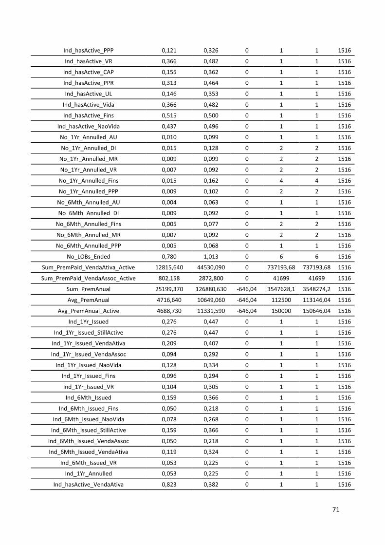
71

Ind_hasActive_PPP 0,121 0,326 0 1 1 1516

Ind_hasActive_VR 0,366 0,482 0 1 1 1516

Ind_hasActive_CAP 0,155 0,362 0 1 1 1516

Ind_hasActive_PPR 0,313 0,464 0 1 1 1516

Ind_hasActive_UL 0,146 0,353 0 1 1 1516

Ind_hasActive_Vida 0,366 0,482 0 1 1 1516

Ind_hasActive_Fins 0,515 0,500 0 1 1 1516

Ind_hasActive_NaoVida 0,437 0,496 0 1 1 1516

No_1Yr_Annulled_AU 0,010 0,099 0 1 1 1516

No_1Yr_Annulled_DI 0,015 0,128 0 2 2 1516

No_1Yr_Annulled_MR 0,009 0,099 0 2 2 1516

No_1Yr_Annulled_VR 0,007 0,092 0 2 2 1516

No_1Yr_Annulled_Fins 0,015 0,162 0 4 4 1516

No_1Yr_Annulled_PPP 0,009 0,102 0 2 2 1516

No_6Mth_Annulled_AU 0,004 0,063 0 1 1 1516

No_6Mth_Annulled_DI 0,009 0,092 0 1 1 1516

No_6Mth_Annulled_Fins 0,005 0,077 0 2 2 1516

No_6Mth_Annulled_MR 0,007 0,092 0 2 2 1516

No_6Mth_Annulled_PPP 0,005 0,068 0 1 1 1516

No_LOBs_Ended 0,780 1,013 0 6 6 1516

Sum_PremPaid_VendaAtiva_Active 12815,640 44530,090 0 737193,68 737193,68 1516

Sum_PremPaid_VendaAssoc_Active 802,158 2872,800 0 41699 41699 1516

Sum_PremAnual 25199,370 126880,630 -646,04 3547628,1 3548274,2 1516

Avg_PremAnual 4716,640 10649,060 -646,04 112500 113146,04 1516

Avg_PremAnual_Active 4688,730 11331,590 -646,04 150000 150646,04 1516

Ind_1Yr_Issued 0,276 0,447 0 1 1 1516

Ind_1Yr_Issued_StillActive 0,276 0,447 0 1 1 1516

Ind_1Yr_Issued_VendaAtiva 0,209 0,407 0 1 1 1516

Ind_1Yr_Issued_VendaAssoc 0,094 0,292 0 1 1 1516

Ind_1Yr_Issued_NaoVida 0,128 0,334 0 1 1 1516

Ind_1Yr_Issued_Fins 0,096 0,294 0 1 1 1516

Ind_1Yr_Issued_VR 0,104 0,305 0 1 1 1516

Ind_6Mth_Issued 0,159 0,366 0 1 1 1516

Ind_6Mth_Issued_Fins 0,050 0,218 0 1 1 1516

Ind_6Mth_Issued_NaoVida 0,078 0,268 0 1 1 1516

Ind_6Mth_Issued_StillActive 0,159 0,366 0 1 1 1516

Ind_6Mth_Issued_VendaAssoc 0,050 0,218 0 1 1 1516

Ind_6Mth_Issued_VendaAtiva 0,119 0,324 0 1 1 1516

Ind_6Mth_Issued_VR 0,053 0,225 0 1 1 1516

Ind_1Yr_Annulled 0,053 0,225 0 1 1 1516

Ind_hasActive_VendaAtiva 0,823 0,382 0 1 1 1516

72

Ind_hasActive_VendaAssoc 0,324 0,468 0 1 1 1516

No_MR_VendaAtiva_Ever 0,199 0,551 0 6 6 1516

No_MR_VendaAssoc_Ever 0,177 0,464 0 8 8 1516

No_MR_VendaAssoc_Active 0,114 0,328 0 2 2 1516

No_MR_VendaAtiva_Active 0,156 0,470 0 6 6 1516

Ind_hasActive_MR_VendaAssoc 0,111 0,314 0 1 1 1516

Ind_hasActive_MR_VendaAtiva 0,126 0,332 0 1 1 1516

No_VR_VendaAtiva_Ever 0,117 0,343 0 3 3 1516

No_VR_VendaAtiva_Active 0,103 0,306 0 2 2 1516

No_VR_VendaAssoc_Ever 0,488 0,847 0 7 7 1516

No_VR_VendaAssoc_Active 0,370 0,648 0 4 4 1516

Ind_hasActive_VR_VendaAtiva 0,102 0,303 0 1 1 1516

Ind_hasActive_VR_VendaAssoc 0,292 0,455 0 1 1 1516

Ind_Sim_Ever 0,514 0,500 0 1 1 1516

Ind_Sim_1Yr 0,239 0,427 0 1 1 1516

Ind_Sim_6Mth 0,135 0,342 0 1 1 1516

Ind_Conv_Ever 0,297 0,457 0 1 1 1516

Ind_Conv_1Yr 0,121 0,327 0 1 1 1516

Ind_Conv_6Mth 0,074 0,262 0 1 1 1516

Ind_Sim_NoConv_Ever 0,217 0,412 0 1 1 1516

Ind_Sim_NoConv_1Yr 0,117 0,322 0 1 1 1516

No_Sim_1Yr 0,399 0,882 0 8 8 1516

No_Conv_1Yr 0,154 0,464 0 4 4 1516

AVG_of_Ind_Prem_GreaterThanAvg 0,311 0,355 0 1 1 1199

AVG_of_Ind_Prem_GreaterThanMedia 0,451 0,374 0 1 1 1199

VAR_23 5,034 2,602 0 9 9 1192

VAR_28 2,745 2,701 0 9 9 1516

VAR_29 1,998 2,327 0 9 9 1516

VAR_30 2,622 2,672 0 9 9 1516

VAR_31 2,906 3,065 0 9 9 1516

VAR_32 2,092 2,392 0 9 9 1516

VAR_42 4,099 3,066 0 9 9 1495

VAR_43 3,035 2,703 0 9 9 1495

VAR_44 5,638 3,062 0 9 9 1516

VAR_45 3,055 3,009 0 9 9 1516

VAR_46 3,418 2,433 0 9 9 1516

VAR_47 2,717 2,802 0 9 9 1516

VAR_49 2,949 2,965 0 9 9 1516

VAR_50 2,615 2,695 0 9 9 1516

VAR_51 2,668 2,742 0 9 9 1516

VAR_52 2,844 2,803 0 9 9 1516

73

VAR_53 3,039 3,096 0 9 9 1516

VAR_54 2,385 2,658 0 9 9 1516

VAR_34 5,307 4,354 2 91 89 1480

VAR_60 0,087 0,282 0 1 1 1516

VAR_61 0,201 0,401 0 1 1 1516

VAR_17 0,599 0,490 0 1 1 1516

VAR_7 0,658 0,475 0 1 1 1516

VAR_9 0,625 0,484 0 1 1 1516

VAR_13 0,577 0,494 0 1 1 1516

VAR_16 0,857 0,350 0 1 1 1516

VAR_10 0,929 0,257 0 1 1 1516

VAR_18 0,779 0,415 0 1 1 1516

VAR_21 0,414 0,493 0 1 1 1516

VAR_19 0,789 0,408 0 1 1 1516

VAR_12 0,637 0,481 0 1 1 1516

VAR_20 0,722 0,448 0 1 1 1516

VAR_14 0,484 0,500 0 1 1 1516

VAR_11 0,695 0,461 0 1 1 1516

VAR_15 0,679 0,467 0 1 1 1516

VAR_58 0,768 0,422 0 1 1 1516

VAR_62 0,924 0,266 0 1 1 1516

VAR_63 0,679 0,467 0 1 1 1516

VAR_70 0,308 0,462 0 1 1 1516

VAR_8 0,561 0,497 0 1 1 1516

Val_CapitalObjecto_N 18,772 29,617 1 339 338 1418

Val_CapitalObjecto_Median 63491,310 45361,790 4976,42 967584,6 962608,18 1418

Ind_Sim_NoConv_6Mth 0,061 0,240 0 1 1 1516

Table 17 –Sample quantitative variables descriptive statistics

Statistic Ensemble Neural

Network Log. Reg.

Dec. Tree

Train: Akaike's Information Criterion 1199,286 806,469

Train: Average Error Function 0,352 0,357

Train: Average Squared Error 0,105 0,114 0,115 0,124

Train: Bin-Based Two-Way Kolmogorov-Smirnov Probability Cutoff

0,557 0,589 0,591 0,55

Train: Bin-Based Two-Way Kolmogorov-Smirnov Statistic 0,704 0,663 0,666 0,646

Train: Cumulative Lift 1,998 1,998 1,998 1,998

Train: Cumulative Percent Captured Response 20,151 20,151 20,151 20,151

Train: Cumulative Percent Response 100 100 100 100

74

Train: Degrees of Freedom for Error 835 1037

Train: Divisor for ASE 2122 2122 2122 2122

Train: Error Function 747,286 758,469

Train: Final Prediction Error 0,176 0,121

Train: Frequency of Classified Cases 1061 1061 1061 1061

Train: Gain 99,812 99,812 99,812 99,812

Train: Gini Coefficient 0,87 0,841 0,836 0,801

Train: Kolmogorov-Smirnov Probability Cutoff 0,48 0,59 0,53 0,51

Train: Kolmogorov-Smirnov Statistic 0,714 0,668 0,681 0,646

Train: Lift 1,998 1,998 1,998 1,998

Train: Maximum Absolute Error 0,924 0,974 0,985 0,9

Train: Mean Square Error 0,145 0,118

Train: Misclassification Rate 0,147 0,176 0,171 0,177

Train: Model Degrees of Freedom 226 24

Train: Number of Estimate Weights 226 24

Train: Number of Wrong Classifications 156 187 181 188

Train: Percent Captured Response 9,981 9,981 9,981 9,981

Train: Percent Response 100 100 100 100

Train: Roc Index 0,935 0,921 0,918 0,901

Train: Root Average Squared Error 0,324 0,337 0,34 0,353

Train: Root Final Prediction Error 0,419 0,348

Train: Root Mean Squared Error 0,38 0,344

Train: Schwarz's Bayesian Criterion 2321,821 925,677

Train: Sum of Case Weights Times Freq 2122 2122

Train: Sum of Frequencies 1061 1061 1061 1061

Train: Sum of Squared Errors 223,243 241,651 245,058 263,718

Train: Total Degrees of Freedom 1061 1061 1061

Valid: Average Error Function 0,4 0,411

Valid: Average Squared Error 0,124 0,129 0,133 0,145

Valid: Bin-Based Two-Way Kolmogorov-Smirnov Probability Cutoff

0,55 0,587 0,576 0,471

Valid: Bin-Based Two-Way Kolmogorov-Smirnov Statistic 0,639 0,639 0,613 0,604

Valid: Cumulative Lift 2,004 2,004 2,004 1,889

Valid: Cumulative Percent Captured Response 20,264 20,264 20,264 19,1

Valid: Cumulative Percent Response 100 100 100 94,253

Valid: Divisor for ASE 910 910 910 910

Valid: Error Function 363,999 373,576

Valid: Frequency of Classified Cases 455 455 455 455

Valid: Gain 100,441 100,441 100,441 88,921

Valid: Gini Coefficient 0,814 0,794 0,784 0,736

Valid: Kolmogorov-Smirnov Probability Cutoff 0,47 0,54 0,55 0,36

Valid: Kolmogorov-Smirnov Statistic 0,653 0,644 0,626 0,609

75

Valid: Lift 2,004 2,004 2,004 1,889

Valid: Maximum Absolute Error 0,976 0,965 0,99 1

Valid: Mean Square Error 0,129 0,133

Valid: Misclassification Rate 0,178 0,191 0,204 0,2

Valid: Number of Wrong Classifications 81 87 93 91

Valid: Percent Captured Response 10,132 10,132 10,132 9,55

Valid: Percent Response 100 100 100 94,253

Valid: Roc Index 0,907 0,897 0,892 0,868

Valid: Root Average Squared Error 0,352 0,359 0,365 0,381

Valid: Root Mean Square Error 0,359 0,365

Valid: Sum of Case Weights Times Freq 910 910

Valid: Sum of Frequencies 455 455 455 455

Valid: Sum of Squared Errors 112,461 117,476 121,4 132,063

Table 18 – Statistics Comparison

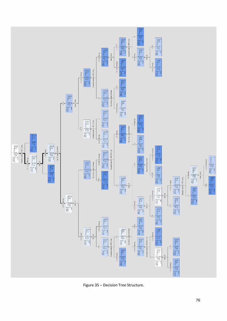
76

Figure 35 – Decision Tree Structure.

77

BIBLIOGRAPHY

A simple explanation of how entropy fuels a decision tree model (2012, Jan 11). Retrieved

from http://www.simafore.com

Agaba, R. (2017, Apr 24). Why Insurance Businesses Need to Use Predictive Analytics.

Retrieved from https://www.ibm.com

Anonymous. (2003). Data Mining Using SAS Enterprise Miner: A Case Study Approach. pp. 1-

84.

Anthony, Martin (2001). Discrete Mathematics of Neural Networks. Threshold Functions. pp.

21-33.

Azevedo, A. & Santos, M. F. (n.d). KDD, SEMMA and CRISP-DM: A Parallel Overview. pp. 1-6.

Berry, M. J. A. and Linoff, G. (1997), Data Mining Techniques for Marketing, Sales, and

Customer Relationship Management. pp. 87-120, 165-254.

Berry, M. J. A. and Linoff, G. (2009), Data Mining Techniques: Theory and Practice. pp. 19-141.

Chattopadhyay, S. (2011). Analytics: A Powerful Tool for the Life Insurance Industry. Using

analytics to acquire and retain customers. pp. 1-8

Christie, P. et al. (2011). Applied Analytics Using SAS Enterprise Miner. Course Notes. pp. 113-

412

Faraway, J. (2006). Extending the Linear Model with R. Chapman & Hall, Parkway, NW. pp. 126-

149.

Georges, J. & Potts, W. (1998). Enterprise Miner: Applying Data Mining Techniques. pp. 1-139.

Georges, J. (2002). Predictive Modeling Using Enterprise Miner. pp. 1-230.

Getting Started with SAS Enterprise Miner 14.1. (2015). Cary, NC. SAS Institute Inc. pp. 9-44.

Guzman, L. (2015). Data sampling improvement by developing SMOTE technique in SAS. pp. 1-

9.

Han, J., Kamber, M., & Pei Jian. (2012). Data Mining Concepts and Techniques: Elsevier. pp.

327-439.

Hand, D., Mannila, H. & Smyth, P. (2001). Principles of Data Mining. Predictive Modeling for A

simple explanation of how entropy fuels a decision tree model (2012, Jan 11). Retrieved from

http://www.simafore.com

Agaba, R. (2017, Apr 24). Why Insurance Businesses Need to Use Predictive Analytics.

Retrieved from https://www.ibm.com

Anonymous. (2003). Data Mining Using SAS Enterprise Miner: A Case Study Approach. pp. 1-

84.

78

Anthony, Martin (2001). Discrete Mathematics of Neural Networks. Threshold Functions. pp.

21-33.

Azevedo, A. & Santos, M. F. (n.d). KDD, SEMMA and CRISP-DM: A Parallel Overview. pp. 1-6.

Berry, M. J. A. and Linoff, G. (1997), Data Mining Techniques for Marketing, Sales, and

Customer Relationship Management. pp. 87-120, 165-254.

Berry, M. J. A. and Linoff, G. (2009), Data Mining Techniques: Theory and Practice. pp. 19-141.

Chattopadhyay, S. (2011). Analytics: A Powerful Tool for the Life Insurance Industry. Using

analytics to acquire and retain customers. pp. 1-8

Christie, P. et al. (2011). Applied Analytics Using SAS Enterprise Miner. Course Notes. pp. 113-

412

Faraway, J. (2006). Extending the Linear Model with R. Chapman & Hall, Parkway, NW. pp. 126-

149.

Georges, J. & Potts, W. (1998). Enterprise Miner: Applying Data Mining Techniques. pp. 1-139.

Georges, J. (2002). Predictive Modeling Using Enterprise Miner. pp. 1-230.

Getting Started with SAS Enterprise Miner 14.1. (2015). Cary, NC. SAS Institute Inc. pp. 9-44.

Guzman, L. (2015). Data sampling improvement by developing SMOTE technique in SAS. pp. 1-

9.

Han, J., Kamber, M., & Pei Jian. (2012). Data Mining Concepts and Techniques: Elsevier. pp.

327-439.

Hand, D., Mannila, H. & Smyth, P. (2001). Principles of Data Mining. Predictive Modeling for

Classification. The MIT Press, Cambridge, MA.

Hastie, T., Tibshirani, R. & Friedman J. (2008). The Elements of Statistical Learning. Data

Mining, Inference, and Prediction. 101-135, 308-310, 605-622.

Hobbs, G. (n.d.). Decision Trees as a Predictive Modeling Method. pp. 1-8.

Hosmer, David W., & Lemeshow, Stanley, (1989). Applied Logistic Regression. The Multiple

Logistic Regression Model. pp. 25-37.

Hossin, M. & Sulaiman, M. (2015). A Review on Evaluation Metrics for Data Classification

Evaluations. International Journal of Data Mining & Knowledge Management Process (IJDKP)

Vol.5, No.2. pp. 1-11

Immadi, M. & Chakraborty G. (2012). Kass Adjustments in Decision Trees on Binary/Interval

Target. pp. 1-9.

Jensen, D. & Schimill, M. (1997). Adjusting for Multiple Comparisons in Decision Tree Pruning.

pp. 1-4.

79

Kotu, V. & Deshpande, B. (2015). Predictive Analytics and Data Mining. pp. 65-164.

Lantz, B. (2015). Machine Learning with R. Waltham, MA, Packt Publishing. pp. 125-169, 311-

363.

Lavery, R. & Mawr, B. (2016). An Animated Guide: Deep Neural Networks in SAS Enterprise

Miner. pp. 1-47

Law, D. & Butler, S. (2014). Insurance 2020: The digital prize – Taking customer connection to a

new level. pp. 1-24.

Lee, P. & Guven, S. (2012, March). The Future of Predictive Modeling: Man Versus Machine.

Retrieved from https://www.towerswatson.com

Maimon, O. & Rokach, L. Data Mining and Knowledge Discovery Handbook. Springer, Berlin,

Germany. pp. 152-288.

Mauboussin, M., Calahan, D. (2015). Sharpening Your Forecasting Skills. Foresight Is a

Measurable Skill That You Can Cultivate. pp. 6-10.

Milanović, M. & Stamenković, M. (2017), Chaid Decision Tree: Methodological Frame and

Application. pp. 1-24

Miley, H. A., Seabolt, J. D. & Williams, J. S. (1998). Data Mining and the Case for Sampling.

Solving Business Problems Using SAS Enterprise Miner Software. pp. 2-6, 16-21.

Nyce, C. (2007). Predictive Analytics White Paper. pp. 1-24

Olsen, D. L. & Delen, D. (2008). Avanced Data Mining Techniques. Data Mining Processes. pp.

9-34.

Opitz, D., Maclin, R. (1999). Popular Ensemble Methods: An Empirical Study. pp. 1-30.

Rokach, L. & Maimon, O. (2015). Data Mining With Decision Trees. Popular Decision Trees

Induction Algorithms. pp. 77-81.

Sayad, S. Decision Tree - Classification (n.d.). Retrieved from

http://www.saedsayad.com/decision_tree.htm

Solokolova, M. & Lapalme, G. (2009). A systematic analysis of performance measures for

classification tasks. pp. 429-431

Stanley, R. (2017, Jul 26). The Most Important Algorithms for Marketing Data Analysts to

Understand. Retrieved from https://callminer.com

Truxillo, C. & Hogan, C. (2017). Leading with Analytics. pp. 24-80.

Truxillo, C. (2012). Advanced Business Analytics. Predictive Modeling. pp. 297-431

Wang, R., Lee, N. & Wei, Y. (2015). A Case Study: Improve Classification of Rare Events with

SAS Enterprise Miner. pp. 1-12.

80

Wielenga, D.(2007).Identifying and Overcoming Common Data Mining Mistakes. SAS Institute,

Cary, NC. pp. 6-11.

Yan, J., Masud, M. & Cheng-Sheng. W. (2008). Staying Ahead of the Analytical Competitive

Curve: Integrating the Broad Range Applications of Predictive Modeling in a Competitive

Market Environment. pp. 1-15.