IM PROPRIETARY

This document is privileged and proprietary. Redistribution is not authorized without permission of

IntegrityM.

Predictive Modeling Using Logistic Regression

Step-by-Step Instructions

This document is accompanied by the following Excel Template

IntegrityM Predictive Modeling Using Logistic Regression in Excel Template.xlsx

Two datasets are used to run predictive modeling based on prior information:

Training dataset - This dataset includes both historical and current data with distinction of the

outcomes – coded 1 for “Yes” and 0 for “No”. Steps 1 to 7 use the dataset to assess the relative

importance of indicators/variables to the outcome (Weights) and to determine the strength of

their association with the outcome (P-values).

Scoring dataset - new data on individuals/entities/IDs used to compute the probability of

outcome.

Step 1:

Input your analytical file; in our example, we downloaded data from the Office of Inspector General List

of Excluded Individuals and Entities (LEIE) and from the Centers for Medicare and Medicaid Services

(CMS) Public Use File (PUF). Columns A to G of the spreadsheet “Predictive Model” display the data.

The analytical file includes columns A to G. Column A displays the provider identifier and columns B to G

show summary information on the variables per provider inputted to the analysis, including the

response variable informing if the provider was excluded or not (coded “1’ or “0” respectively). The

working dataset consists of information stored in cells B2 to G92.

Steps 2 and 3:

Copy values from column H (RANDBETWEEN Values) to column I (P (E)) – this is necessary because of the

volatile nature of the formula in column H, which will values changed every time the spreadsheet is

refreshed. The rest of the columns in Step 3 will be computed automatically by the formulas embedded

in them (Column J (Odds Ratio), Colum K (If Odds Ratio < 0.1 set it to 0.1) and Column L (Log (Odds Ratio))

The Excel function RANDBETWEEN assigns random probability numbers to the providers

according to their original classification (“1” or “0”) - drawing from the range 0.50 to 0.99 for

providers coded 1 (excluded) and from the range 0.01 to 0.49 for providers coded 0 (active in the

health care program)

Note that the RANDBETWEEN function requires as input values integers (numbers) that define

the bottom and the top values from which a random number will be drawn. The values will be

stored in column H, “RANDBETWEEN Values”. The assigned values need to be transformed to

probability numbers by dividing the function output number by 100 according to the provider

exclusion status and the following Excel operation:

for excluded providers, =RANDBERWEEN(50, 99)/100;

for non-excluded (active) providers, =RANDBERWEEN(1, 49)/100;

IM PROPRIETARY

This document is privileged and proprietary. Redistribution is not authorized without permission of

IntegrityM.

Step 4:

Step 4.1:

o Run the Linear Regression Model by using the Data Analysis tool of Excel as shown in the

screenshot below to obtain the Initial weights (coefficients) of the variables/indicators (in

our example, 5 variables). The regression input Y Range (response variable) is the

“Log(Odds)”, column L; and the five indicators in Input X Range are all values in “PMT per

Bene”, “Services per Bene”, “Average Age of Beneficiaries”, “Beneficiary cc diab percent”

and “Average HCC Risk Score of Beneficiary” – columns C to G. The Regression Model

results will generate a new tab – labeled in our example “Step 4 - Reg Initial Values”.

Step 4.2:

o Copy the coefficients (weights) in column B from the regression model output to the

Coefficients Table (in our example, the table includes cells T3 to T8 in column T of the

spreadsheet “Predictive Model”).

IM PROPRIETARY

This document is privileged and proprietary. Redistribution is not authorized without permission of

IntegrityM.

Step 5:

Update the formula in Column N (variable labeled L) if you have more or less than the 5 variables that we

have in our example. This formula includes the initial values of the weights from the Coefficients Table

(Column T in our example) multiplied by the corresponding indicators (columns C to G in our example).

Changes in the set of summation terms in the cases of 4 or 6 variables would be

4 variables, formula =T$3 + T$4*C4 + T$5*D4 + T$6*E4 + T$7*F4 + T$8*G4

6 variables, formula = T$3 + T$4*C4 + T$5*D4 + T$6*E4 + T$7*F4 + T$8*G4+T$9*H4

IM PROPRIETARY

This document is privileged and proprietary. Redistribution is not authorized without permission of

IntegrityM.

Note: the mathematical constant “e” (=2.7183 in cell T10 in our example) is required to compute the results in column O (labeled eL = "e to power L").

The values of column P (P(X) = eL/(1 + eL)) and column Q (Y*ln[P(X)] + (1 – Y)*ln[1 – P(X)]) will be updated automatically (where Y = 1 for excluded providers and Y = 0 for active providers) by the embedded formulas. Step 6:

Step 6.1: o Update the summation of the Log (Maximum Likelihood) if you have more rows than our

example: If you have 100 rows in your data rather than the 90 rows of our example, change

the formula from =SUM(Q3:Q92) to =SUM(Q3:Q102)

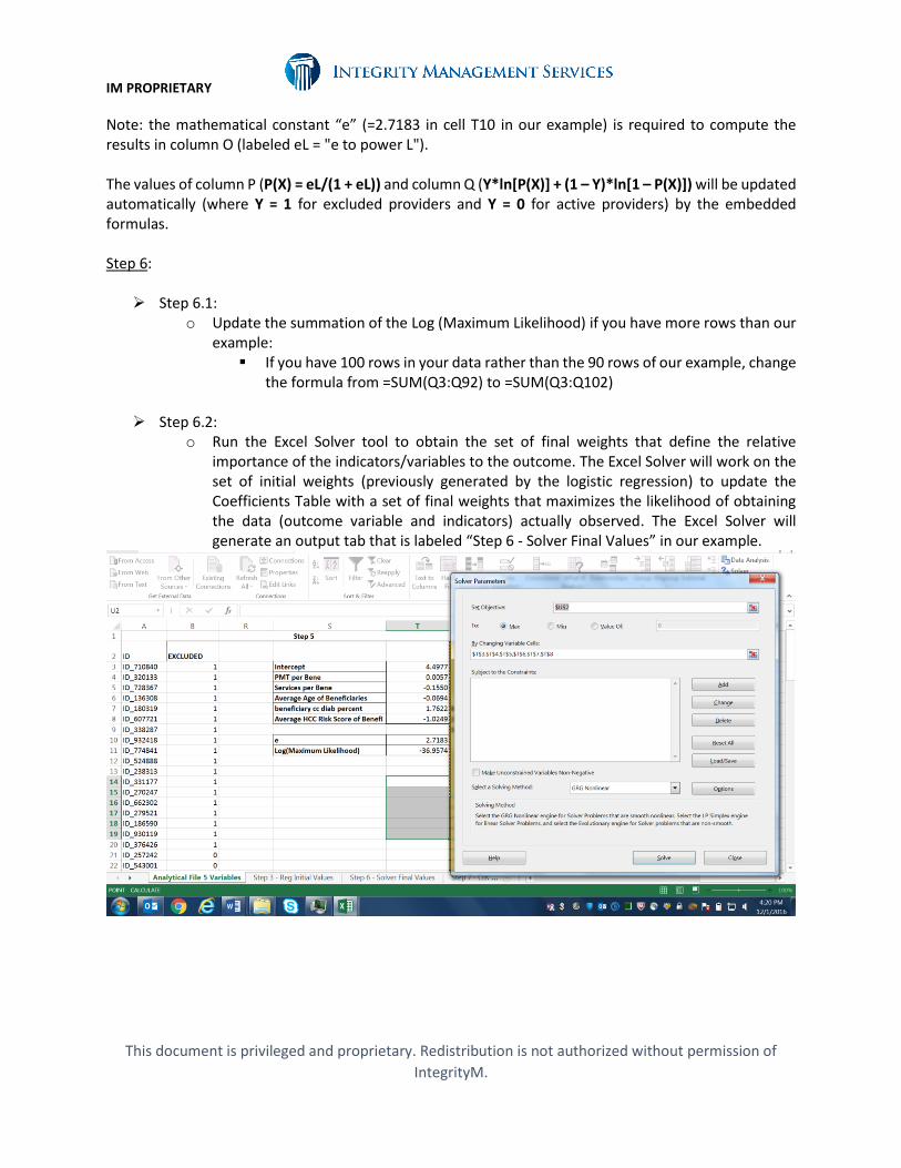
Step 6.2: o Run the Excel Solver tool to obtain the set of final weights that define the relative

importance of the indicators/variables to the outcome. The Excel Solver will work on the set of initial weights (previously generated by the logistic regression) to update the Coefficients Table with a set of final weights that maximizes the likelihood of obtaining the data (outcome variable and indicators) actually observed. The Excel Solver will generate an output tab that is labeled “Step 6 - Solver Final Values” in our example.

IM PROPRIETARY

This document is privileged and proprietary. Redistribution is not authorized without permission of

IntegrityM.

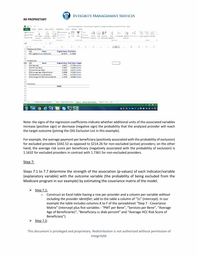
Note: the signs of the regression coefficients indicate whether additional units of the associated variables increase (positive sign) or decrease (negative sign) the probability that the analyzed provider will reach the target outcome (joining the OIG Exclusion List in this example).

For example, the average payment per beneficiary (positively associated with the probability of exclusion) for excluded providers $342.52 as opposed to $214.26 for non-excluded (active) providers; on the other hand, the average risk score per beneficiary (negatively associated with the probability of exclusion) is 1.1632 for excluded providers in contrast with 1.7361 for non-excluded providers.

Step 7: Steps 7.1 to 7.7 determine the strength of the association (p-values) of each Indicator/variable (explanatory variable) with the outcome variable (the probability of being excluded from the Medicare program in our example) by estimating the covariance matrix of the model.

Step 7.1: o Construct an Excel table having a row per provider and a column per variable without

including the provider identifier; add to the table a column of “1s” (intercept). In our example the table includes columns A to F of the spreadsheet “Step 7 - Covariance Matrix” (intercept plus five variables - “PMT per Bene”, “Services per Bene”, “Average Age of Beneficiaries”, “Beneficiary cc diab percent” and “Average HCC Risk Score of Beneficiary”).

Step 7.2:

IM PROPRIETARY

This document is privileged and proprietary. Redistribution is not authorized without permission of

IntegrityM.

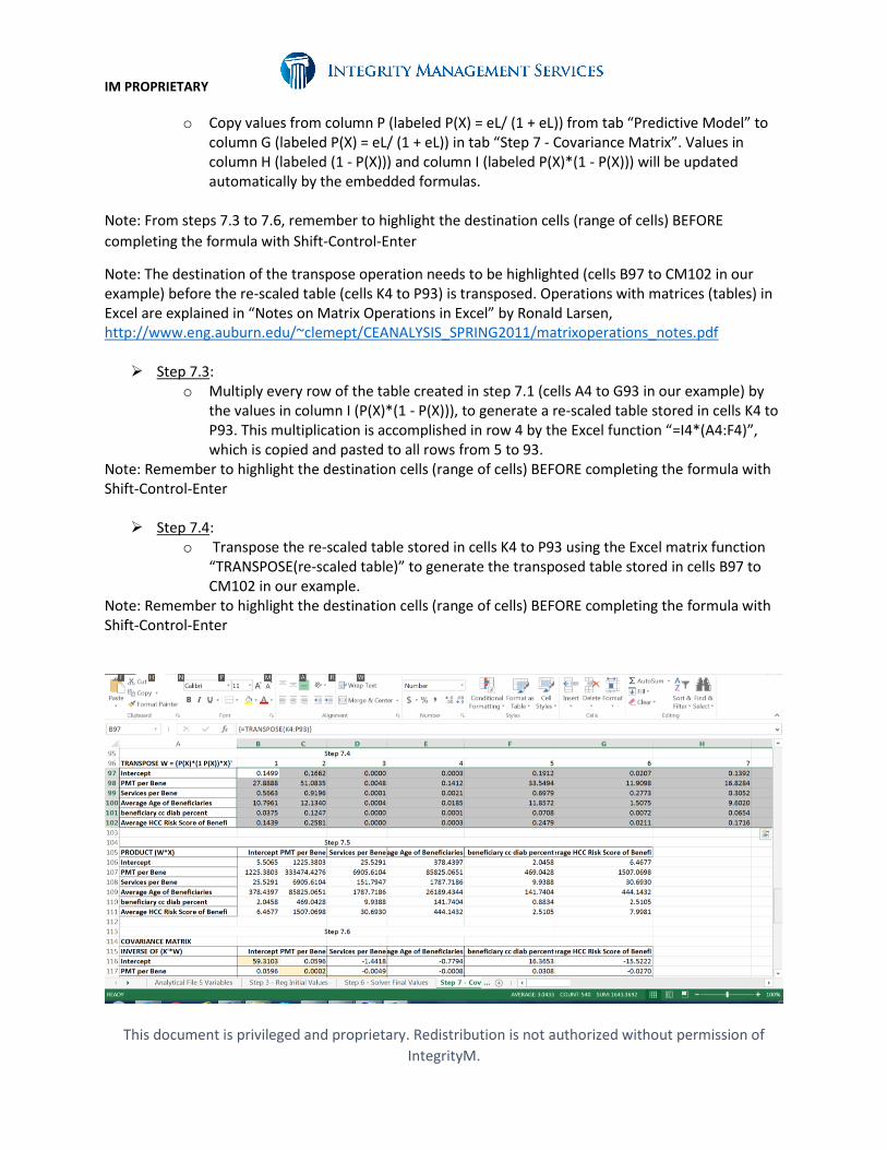
o Copy values from column P (labeled P(X) = eL/ (1 + eL)) from tab “Predictive Model” to column G (labeled P(X) = eL/ (1 + eL)) in tab “Step 7 - Covariance Matrix”. Values in column H (labeled (1 - P(X))) and column I (labeled P(X)*(1 - P(X))) will be updated automatically by the embedded formulas.

Note: From steps 7.3 to 7.6, remember to highlight the destination cells (range of cells) BEFORE

completing the formula with Shift-Control-Enter

Note: The destination of the transpose operation needs to be highlighted (cells B97 to CM102 in our example) before the re-scaled table (cells K4 to P93) is transposed. Operations with matrices (tables) in Excel are explained in “Notes on Matrix Operations in Excel” by Ronald Larsen, http://www.eng.auburn.edu/~clemept/CEANALYSIS_SPRING2011/matrixoperations_notes.pdf

Step 7.3: o Multiply every row of the table created in step 7.1 (cells A4 to G93 in our example) by

the values in column I (P(X)*(1 - P(X))), to generate a re-scaled table stored in cells K4 to P93. This multiplication is accomplished in row 4 by the Excel function “=I4*(A4:F4)”, which is copied and pasted to all rows from 5 to 93.

Note: Remember to highlight the destination cells (range of cells) BEFORE completing the formula with Shift-Control-Enter

Step 7.4: o Transpose the re-scaled table stored in cells K4 to P93 using the Excel matrix function

“TRANSPOSE(re-scaled table)” to generate the transposed table stored in cells B97 to CM102 in our example.

Note: Remember to highlight the destination cells (range of cells) BEFORE completing the formula with Shift-Control-Enter

IM PROPRIETARY

This document is privileged and proprietary. Redistribution is not authorized without permission of

IntegrityM.

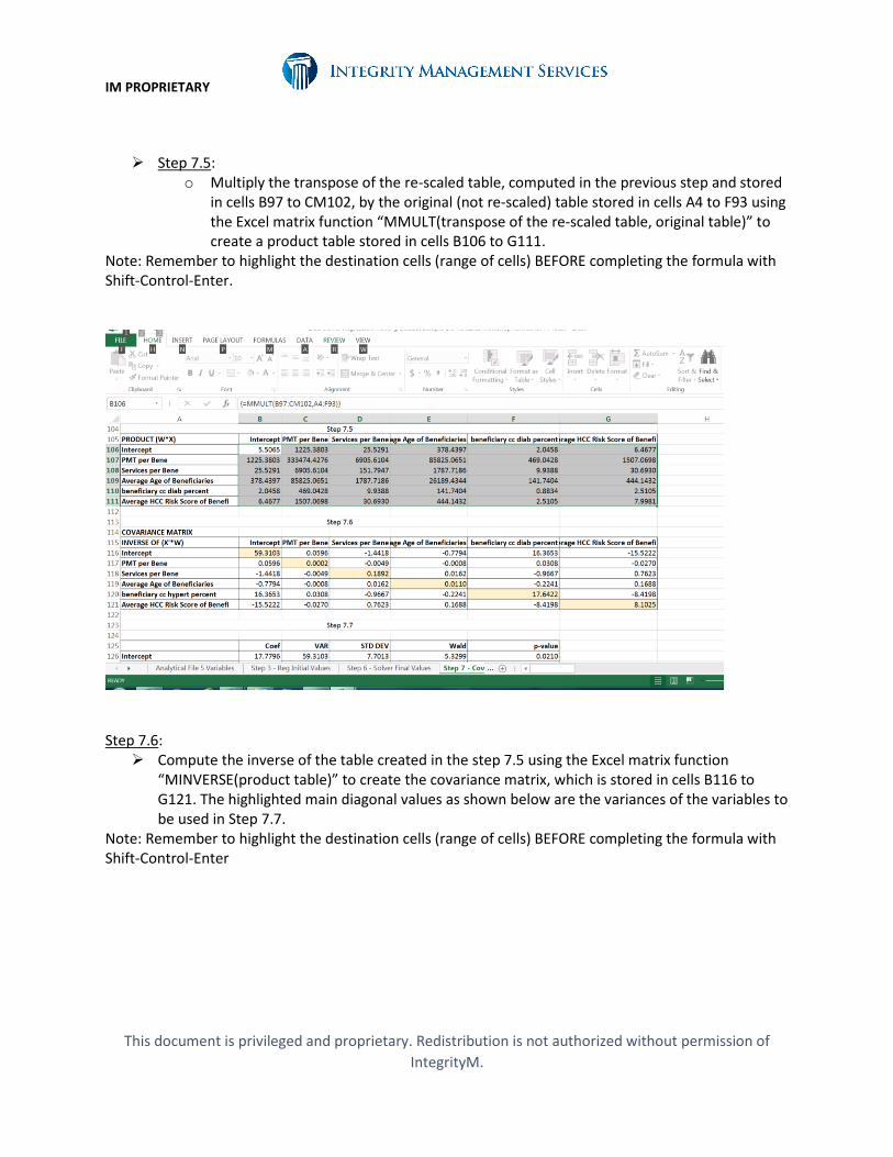
Step 7.5: o Multiply the transpose of the re-scaled table, computed in the previous step and stored

in cells B97 to CM102, by the original (not re-scaled) table stored in cells A4 to F93 using the Excel matrix function “MMULT(transpose of the re-scaled table, original table)” to create a product table stored in cells B106 to G111.

Note: Remember to highlight the destination cells (range of cells) BEFORE completing the formula with Shift-Control-Enter.

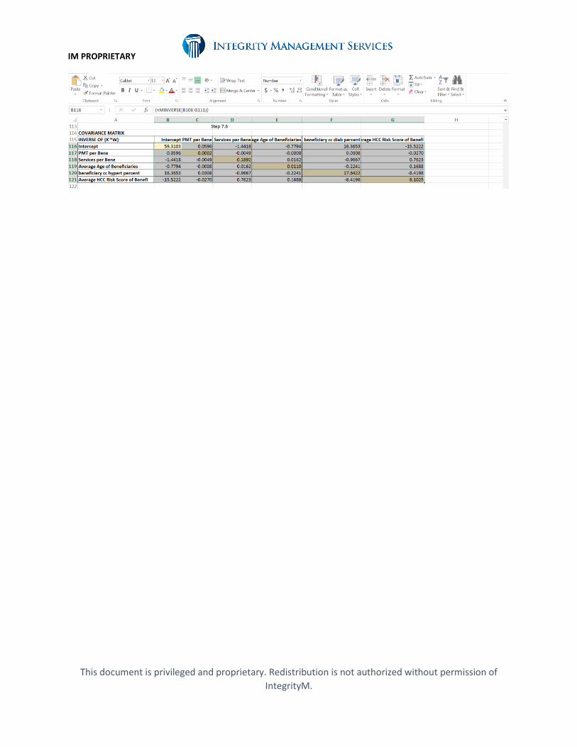
Step 7.6:

Compute the inverse of the table created in the step 7.5 using the Excel matrix function “MINVERSE(product table)” to create the covariance matrix, which is stored in cells B116 to G121. The highlighted main diagonal values as shown below are the variances of the variables to be used in Step 7.7.

Note: Remember to highlight the destination cells (range of cells) BEFORE completing the formula with Shift-Control-Enter

IM PROPRIETARY

This document is privileged and proprietary. Redistribution is not authorized without permission of

IntegrityM.

IM PROPRIETARY

This document is privileged and proprietary. Redistribution is not authorized without permission of

IntegrityM.

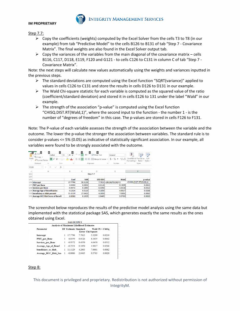
Step 7.7: Copy the coefficients (weights) computed by the Excel Solver from the cells T3 to T8 (in our

example) from tab “Predictive Model” to the cells B126 to B131 of tab “Step 7 - Covariance Matrix”. The final weights are also found in the Excel Solver output tab.

Copy the variances of the variables from the main diagonal of the covariance matrix – cells B116, C117, D118, E119, F120 and G121 - to cells C126 to C131 in column C of tab “Step 7 - Covariance Matrix”.

Note: the next steps will calculate new values automatically using the weights and variances inputted in the previous steps.

The standard deviations are computed using the Excel function “SQRT(variance)” applied to values in cells C126 to C131 and store the results in cells D126 to D131 in our example.

The Wald Chi-square statistic for each variable is computed as the squared value of the ratio (coefficient/standard deviation) and stored it in cells E126 to 131 under the label “Wald” in our example.

The strength of the association “p-value” is computed using the Excel function “CHISQ.DIST.RT(Wald,1)”, where the second input to the function - the number 1 - is the number of “degrees of freedom” in this case. The p-values are stored in cells F126 to F131.

Note: The P-value of each variable assesses the strength of the association between the variable and the

outcome. The lower the p-value the stronger the association between variables. The standard rule is to

consider p-values <= 5% (0.05) as indicative of statistically significant association. In our example, all

variables were found to be strongly associated with the outcome.

The screenshot below reproduces the results of the predictive model analysis using the same data but implemented with the statistical package SAS, which generates exactly the same results as the ones obtained using Excel.

Step 8:

IM PROPRIETARY

This document is privileged and proprietary. Redistribution is not authorized without permission of

IntegrityM.

Steps 8 to 10 use a new dataset of active (unclassified as excluded) providers to score their probability of joining the OIG Exclusion List

Step 8.1: o Input your Scoring dataset - our example used a sample of 100 non-excluded providers.

The dataset included the 5 indicators and used the final weights to score their probability of being excluded. The final weights are inputted in columns K to P in our example.

Step 8.2: o The formulas embedded in columns G to I will generate values based on the data

inputted. Note: the value of the mathematical constant “e” (= 2.7183, copied to the cell N3) is used to compute values in column G (labeled L). The probabilities of exclusion P(X) of provider in row 2 are generated by using the formula “=H2/(1 + H2)”, where the values of H2 are computed in the previous operation.