C S I R O L A N D a nd WAT E R

Prediction of Sheet and Rill Erosion Over the

Australian Continent, Incorporating Monthly

Soil Loss Distribution

Hua Lu, John Gallant, Ian P. Prosser, Chris Moran, Graeme Priestley

CSIRO Land and Water

Technical Report 13/01, May 2001

National Land & Water Resource Audit

A p r o g r a m o f t h e N a t u r a l H e r i t a g e T r u s t

Prediction of Sheet and Rill Erosion Over

the Australian Continent, Incorporating

Monthly Soil Loss Distribution

Hua Lu, John Gallant, Ian P. Prosser, Chris Moran, Graeme Priestley

CSIRO Land and Water Technical Report 13/01

May 2001

ii

© 2001 CSIRO Australia, All Rights Reserved

This work is copyright. It may be reproduced in whole or in part for study,research or training purposes subject to the inclusion of an acknowledgement ofthe source. Reproduction for commercial usage or sale purpose requires writtenpermission of CSIRO Australia

Authors

Hua Lu, John Gallant, Ian P. Prosser, Chris Moran, Graeme Priestley

CSIRO Land and Water, PO Box 1666, Canberra, 2601, Australia

E-mail: hua.lu@cbr.clw.csiro.au

Phone: 61-2-6246-5923

For bibliographic purposes, this document may be cited as:Lu, H., Gallant, J., Prosser, I.P., Moran, C., and Priestley, G. (2001), Predictionof Sheet and Rill Erosion Over the Australian Continent, Incorporating MonthlySoil Loss Distribution. Technical Report 13/01, CSIRO Land and Water,Canberra, Australia.

A PDF version is available athttp://www.clw.csiro.au/publications/technical2001/tr13-01

iii

Contents

ABSTRACT..................................................................................................................................... IV

1 INTRODUCTION .......................................................................................................................1

2 METHODOLOGY ......................................................................................................................2

2.1 Rainfall erosivity ( R ) ..........................................................................................................4

2.2 Soil erodibility ( K ) ..............................................................................................................7

2.3 Cover and crop management factor ( C ) ...........................................................................9

2.4 Slope length factor ( L ) and slope steepness factor ( S ) .................................................16

2.5 Support practise factor ( P ) ..............................................................................................19

3 RESULTS ................................................................................................................................19

3.1 Current Erosion ..................................................................................................................19

3.2 Prediction Evaluation of Current Hillslope Erosion........................................................21

3.3 Erosion Rate between Current and Pre-European Settlement....................................... 23

4 DISCUSSIONS AND CONCLUSIONS ...................................................................................25

5 ACKNOWLEDGEMENTS ......................................................................................................27

6 REFERENCES...........................................................................................................................28

iv

ABSTRACT

A major issue in Australian land management is soil erosion and the consequent

reduction of productivity. The off-site effect of soil erosion is the degradation of

water quality in streams and water storages. Measurement of soil erosion is time

consuming and data on soil erosion rate is limited to a few sites. Those sparse

measurements provide little information about the spatial distribution of soil

loss rate across the nation. This report describes a spatial modelling framework

which is used to predict an Australia-wide sheet and rill erosion. It is based on

the Revised Universal Soil Loss Equation (RUSLE) using time series of remote

sensing imagery and daily rainfall combining with updated spatial data for soil,

land use and topography. The results are presented as a geo-referenced annual

averaged soil loss map and its monthly distributions. It is found that the north

part of the country has higher erosion potential than the south of the country.

The prediction confirms that agricultural land use has higher erosion rate

compared with most natural vegetated lands and that erosion potential differs

significantly between summer and winter periods.

1 INTRODUCTION

Soil erosion caused by rainfall and runoff is recognised as a major

environmental problem in Australia. Suspended sediment concentrations in

streams and lakes affect water use and ecosystem health. High concentrations of

sediment reduce stream clarity, inhibit respiration and feeding of stream biota,

diminish light needed for plant photosynthesis, and require treatment for human

water use. To minimise the decline of soil productivity and water quality and to

optimise the use of resources for soil conservation, spatially distributed patterns

of the hazard sources and associated soil loss rate is essential to identify crucial

areas appropriate for more detailed investigation. Furthermore, the basic

prerequisite for understanding the consequences of changes in land use and

climate on soil erosion is to know the sources and rates of erosion rate under the

present land use and climate conditions.

For the scale under consideration, a simplified version of the Revised Universal

Soil Loss Equation (RUSLE) calibrated using New South Wales field data, was

selected. Application of the RUSLE for the Australian continent affords the

following advantages:

1. It requires a modest amount of parameters that can be derived for a continent

and has been adapted to Australian conditions;

2. Used in conjunction with raster-based GIS, the RUSLE predicts erosion

potential on a cell by cell basis for mapping spatial patterns; and

3. The factor-based nature of the RUSLE allows easy analysis of the role of

individual factors in contributing to the estimated erosion rate.

A similar approach has been applied to the Australian continent before

(Rosewell, 1996), as part of the 1996 National State of the Environment Report.

This assessment provides a significant update on that assessment by inclusion of

improved or new national datasets on rainfall, soils, vegetation cover, land use,

and topography which were not available in 1996. Furthermore, we have been

2

able to incorporate seasonal patterns of rainfall and cover factors, which

Rosewell (1997) suggested was needed for more accurate distinction of the

continental pattern of soil erosion.

In this study, we present a spatial modelling framework designed for the

Australian continent hillslope sheet and rill erosion prediction. Data used to

generate the RUSLE variables include:

1. 13 years NOAA/NASA Pathfinder GAC 8km Advanced Very High

Resolution Radiometer (AVHRR) derived 10-day maximum composite

Normalised Difference Vegetation Index (NDVI) data (Data source: CSIRO

Earth Observation Centre (EOC));

2. 20 years of daily rainfall interpolated from station measurements (Data

source: Queensland Department of Natural Resources (QDNR));

3. Updated national soil attributes maps (Data source: Australian Soil Resource

Information System (ASRIS) project, National Land and Water Resources

Audit (NLWRA));

4. 1 km resolution National landuse map based on 1997 landuse distribution

(Data source: Bureau of Rural Sciences (BRS) and NLWRA),

5. 9” National digital elevation model (DEM) (Data source: AUSLIG); and

6. Locally available higher resolution DEMs (Data source: CSIRO and State

Agencies).

The updated soil attribute maps and the land use map together with this

assessment of soil erosion are products of NLWRA.

2 METHODOLOGY

The RUSLE calculates mean annual soil loss (Y, t ha-1 yr-1) as a product of six

factors: rainfall erosivity factor (R), soil erodibility factor (K), hillslope length

factor (L), hillslope gradient factor (S), ground cover factor (C) and supporting

practice factor (P):

Y = R K L S C P (1)

3

The factors included in the RUSLE vary strongly across the Australia. Using

available spatial information for each factor provides a means for estimating the

spatial patterns of continental scale sheet and rill erosion. Due to lack of spatial

data of contour cultivation and bank systems, an assessment of the supporting

practice factor (P) is excluded.

The precise form of each factor is based on soil loss measurements on hillslope

plots, mainly in the USA. Limited plot scale measurements of erosion have

been undertaken in Australia (e.g. Edwards, 1987; McIvor et al., 1995; Scanlan

et al., 1996) allowing limited local calibration of the USLE factors, particularly

the C factor.

Mean annual values for rainfall erosivity and the cover factor are often used in

direct application of Equation (1) to calculate mean annual hillslope erosion.

This often neglects important seasonal patterns of rainfall erosivity and cover.

Problematic to the standard annual application of the RUSLE is the pronounced

wet-dry precipitation regime in Australian tropics and Mediterranean climate

dominant areas such as south Western Australia. To adequately represent the

erosive potential of rainfall for each temporally distinctive period, this study

applies the RUSLE model on a monthly averaged basis by calculating

appropriate erosivity and cover factors for each month. It can be shown that

incorporation of seasonal effects reduces predicted mean annual soil loss in the

tropics by a factor of 1.5. The modifications of Equation (1) discussed above

yield monthly soil loss rate which can be calculated as:

jjj CSLKRY = (2)

where ,12

1∑

=

=

j

jjj R

RSLRC Rj and SLRj are cover management factor, rainfall

erosivity and the soil loss ratio, respectively, for month j.

Sections 2.1 – 2.5 describe the calculation procedure for each factor in Equation

(2). The calculation was applied for each grid cell at an appropriate resolution

determined by the source data resolution. More specifically, 0.05° for R factor

4

determined by QDNR daily rainfall data, 0.01° for C factor determined by the

NLWRA/BRS landuse data, 0.0025° for LS factor determined by the 9”

AUSLIG DEM, and 0.0025° for K factor determined by the ASRIS soil

attributes. The resulted images with resolution coarser than 9” were re-sampled

to 0.0025°, which is NLWRA Theme 5.4b, sediment delivery and transport

project required resolution. The bilinear option was used to re-sample R factor

and its monthly distributions and the nearest neighbour option was used for C

factor re-sampling. All the images were then extended to the coast line using

nibble command in ARC/INFO. The re-sampled images were finally multiplied

using Equation (2) to produce monthly hillslope erosion rate (in the unit of t ha-1

yr-1) maps. The annual hillslope erosion map is the sum of the twelve monthly

erosion maps.

2.1 Rainfall erosivity (R)

Rainfall erosivity (R) is defined as the mean annual sum of individual storm

erosion index values, EI30 , where E is the total storm kinetic energy and I30 is

the maximum rainfall intensity in 30 minutes. To compute storm EI30,

continuous rainfall intensity data are needed. Wischmeier and Smith (1978)

recommended that at least 20 years of pluviograph data be used to accommodate

natural climatic variations. However, the spatial and temporal coverage of

pluviograph data is often very limited.

Yu and Rosewell (1996a, 1996b) and Yu (1998) proposed a rainfall erosivity

model in which storm EI30 for the month j is related to daily rainfall amount, Rd,

in the form:

[ ] 01

30 )2cos(1)( RRRjfjEI d

N

dd >−+= ∑

=

βωπηα (3)

where Rd is the daily rainfall amount, R0 is the threshold rainfall amount to

generate runoff (set to 12.7 mm; Wischmeier and Smith, 1978), and N is the

number of days with rainfall amount in excess of R0 in the month. The first part

of the equation is a sinusoidal function with a wavelength of twelve months (f =

1/12). It is used to describe the seasonal variation of rainfall erosivity for a

5

given amount of daily rainfall. The parameter ω is set at π/6, implying that for

a given amount of daily rainfall the corresponding rainfall erosivity is the

highest in January, when the temperature is the highest for most part of the

continent. Regional relationships were derived using 79 stations located in

NSW, SA, and the tropics for parameters α, β, η :

α = 0.395 [1 + 0.098 exp(3.26 Ψ/Μ)]

β = 1.49

η = 0.29

where Μ is the mean annual rainfall and Ψ is the mean summer rainfall

(November to April; Bureau of Meteorology 1989).

The model was applied to the Australian continent using 0.05° resolution daily

rainfall data interpolated by Queensland Department of Natural Resources. The

description of daily rainfall interpolation can be found in Jeffrey et al. (2001).

Ordinary kriging is firstly used to spatially interpolate monthly rainfall values.

Then, for each grid cell, the daily distribution of rainfall throughout the month is

calculated by accessing the rainfall record for the station nearest the points of

interest, and partitioning the interpolated monthly rainfall onto individual days

according to the long-term distribution of daily rainfall at the nearest rain gauge

station. In this study, 20 years of grided daily rainfall from 1st of January, 1980

to 31st of December, 1999 are used. The ratio Ψ/Μ was calculated using the

same daily rainfall data. The resulting rainfall erosivities calculated are the mean

annual R factor (averaged annual EI30 ), and mean monthly R factors for the 20

year period.

The R factor, estimated using the daily model, and that of several previous

researchers (McFarlane et al., 1986; Rosenthal and White, 1980; Yu and

Rosewell, 1996a,b; Yu, 1998) have been compared for 120 stations across

Australia. Figure 1 shows the comparison between the modelled and actual R

factor. The linear correlation coefficient (Pearson’s r) is 0.903 (SSE = 5.1e8, σ

= 1909.5). The standard deviation of measured R is 4311 and 4428 for predicted

6

R. No noticeable bias of the model is observed. In general, the model compares

well with various R factors calculated using pluviograph data.

The estimated spatial pattern of the R factor and the monthly distributions for

selected locations across the continent are shown in Figure 2. For the northern

Figure 1. Comparison between modelled and actual R factor for 142 points at120 locations (shown in the bottom map, with references to the ILZ and theNLWRA defined regions). Multiple values for the same rainfall gauge stationgiven by different authors using different period of pluviograph data areincluded. 1:1 line (solid blue) is shown. The unit of R factor is MJ mm ha-1 hr-

1 yr-1.

Thursday Island

Coen

Gove

Cairns

Rockhampton

Townsville

Brisban eCoffs Harbo ur

Sydney

NowraAdelaid e Deniliquin

Darwin

NormantonBroo me

Rabbit Flat

Katherine

Daly Waters

Carnarvo n

Albany

Lake G race

Giles

Alice SpringsBoulia

Mitchell

Month of year

Perc

enta

geR

fact

or(%

) Mossman QLD

0

5

10

15

20

25

30

1 2 3 4 5 6 7 8 9 10 11 12

Figure 2. Map of rainfall erosivity (R factor) and its monthly distributions for selected locations.

7

part of the continent, the monthly distributions of R factor estimated using

Equation (3) generally show peaks in summer period, from December to

February. Approximately 80% of the annual rainfall erosivity occur between

December and March. A negligible fraction occurs in the months from April to

October in northern Australia. This is consistent with the common rainfall

pattern in the Australia’s tropics of intense storms during summer and little

rainfall during winter (McIvor et al., 1995; Rosenthal and White, 1980). For the

south-eastern part of the continent, predicted monthly R factor distributions

change gradually from summer dominance to uniform when moving from north

to south, which is comparable with continent rainfall intensity distribution

(Bureau of Meteorology, 1989; Yu and Rosewell, 1996a,b; Yu 1998). Winter

dominant monthly R factor distributions are obtained for the coast area of

southwestern part of Western Australia. The pattern then changes to a summer

dominance inland within one hundred kilometres from the coast (Figure 2). This

is also comparable with the distributions of the R factor estimated using

pluviograph data for the region (McFarlane et al., 1986). Quantitative

assessment of the monthly distribution of R factor is technically challenging as

many previously existing R factors were calculated using short periods of

pluviograph data. This causes serious bias for monthly distribution of the R

factor toward single large storms in the period.

2.2 Soil erodibility (K)

Soil erodibility (K) is a measure of the susceptibility of the soil to erosion. In the

RUSLE, it is a quantitative value determined experimentally. For a particular

soil, it is the rate of soil loss per erosion index unit as measured on a unit plot

maintained under continuous bare fallow. For satisfactory direct measurement of

soil erodibility, erosion from field plots needs to be studied for periods generally

well in excess of 5 years (Loch et al., 1998). This is costly and time-consuming,

and data from field studies of adequate duration are available for only a few

Australian soils (Loch et al., 1998). Therefore, considerable attention has been

paid to estimate soil erodibility from soil attributes such as particle size

distribution, organic matter content and density of eroded soil (e.g. Wischmeier

8

et al., 1971; Loch and Rosewell, 1992). Even these data, however, are not

readily available at regional or continental scales.

In this study, a modified nomograph equation (Wishmeier et al. 1971) was used

to estimate K factor for Australian soils. The soil erodibility surface has been

generated using the equation (Loch and Rosewell, 1992):

K = 2.77 (100 P125)1.14 (10 -7) (12 - 2 Oc) + 3.29 (10 -3) (Pr - 3)

where P125 is the percentage of particles with diameter less than 0.125 mm, Oc is

organic carbon in percentage, and Pr is the soil permeability rating. These soil

attributes were obtained using data including polygon-based soil information

from various state agencies, the digital Atlas of Australian Soils (Northcote et

al. 1960-1968), and a digital polygon coverage of the Soil-Landforms of the

Murray-Darling Basin. An organic carbon surface is obtained by statistical

modelling using point observations, climatic data, elevation data and

LANDSAT MSS satellite data. Using a look-up table linking unique soil type

described as Principle Profile Form (PPF) with interpreted soil attributes

(McKenzie et al. 2000), a weighted mean approach was taken to average soil

attribute values in each polygon. Based on the area occupied by each PPF, the

final soil attribute value for a polygon was calculated by the addition of the area

weighted soil attribute value for each PPF. Rosewell’s (1993) classes for soil

permeability were used to categorise the saturated hydraulic conductivity of the

A-horizon derived by the Australia Soil Resource Information System (ASRIS)

project of NLWRA. The K factor surface is a product of ASRIS project.

It is found, nationally, that heavy clay soils (Vertosols) are highly erodible as

they are structurally unstable. Relatively large K values are estimated for

chemically dispersible sodic soils (Sodosols). Kandosols and Calcarosols with

sandy topsoil are slightly less erodible. Rocky soils (Rudosols) and weakly

developed soils (Tenosols) are least erodible. Soils with high organic matter

content are less erodible than those with low organic matter content. There is an

obvious state boundary between SA and Victoria, partly due to land

management differences and to original map sources of soil data.

9

2.3 Cover and crop management factor (C)

The cover and crop management factor (C) measures the combined effect of all

the interrelated cover and crop management variables. It is defined as the ratio

of soil loss from land maintained under specified conditions to the

corresponding loss from continuous tilled bare fallow. It is an estimate of the

combined effects of prior land use, crop canopy cover, surface cover, surface

roughness, and organic material below the soil surface. It is usually expressed as

an annual value for a particular cover and crop management system but is

calculated from the soil loss ratios for shorter periods of time within which

cover and management effects are relatively uniform. The soil loss ratios are

combined in proportion to the applicable percentages of erosivity (R) to derive

annual C values. At continental scale, deriving the appropriate C values

essentially requires accurate estimation of canopy cover and ground cover as

they offer very different erosion control protection. Although tree canopy cover

can be estimated at annual averaged basis due to it relatively slow growth, there

are strong seasonal patterns to ground cover in the Australian continent,

reflecting seasonal patterns in rainfall. We, therefore, calculated mean monthly

values of C to reflect seasonal variations in cover. The best way to assess cover

patterns across a large area is by interpretation of remote sensing data because

satellite remote sensing offers the only practical means of continuously and

consistently monitoring vegetation cover on a continent scale.

For each grid cell, the calculation of C factor involves the following distinct

steps:

1. Separating the NDVI signals into three components, perennial NDVI,

seasonal NDVI and random NDVI using time series decomposition;

2. Estimating vegetation covers by regression equations between long-term

annual averaged perennial NDVI and woody cover, and between monthly

averaged seasonal NDVI and ground cover using site measurements;

3. Calculating monthly soil loss ratio (SLR) using a simplified version of

SOILOSS (Rosewell, 1993); and

4. Calculating annual C factor values by weighting SLR with the fraction of

rainfall erosivity (R) associated with the corresponding month.

10

2.3.1 Pathfinder AVHRR NDVI

This NDVI time series was derived from the AVHRR sensor on the National

Oceanographic and Atmospheric Administration (NOAA) series of

meteorological satellites (NOAA–7, -9, and –11) and made available by the

NASA Goddard Space Flight Distributed Active Archive Centre (GDAAC)

(James and Kalluri, 1994). The spatial resolution is 0.08° (approx. 8 km) and the

temporal coverage is 10-day maximum NDVI composite from July 1981

through to the middle of 1994. The Pathfinder NDVI is corrected for change in

sensor calibration, ozone absorption, Rayleigh scattering and normalised for

changes in solar zenith angle. The CSIRO Earth Observation Centre (EOC)

obtained a subset covering the Australian continent from NASA. The NDVI

time series was further noise reduced by using a modified Best Index Slope

Extraction (BISE) algorithm using a search window of 6 decads and a NDVI

change threshold of 0.1 per decad (Lovell and Graetz, 2000). The data set was

Table 1: The NDVI time series used in this study (Note: ULHC is upper lefthand corner, BRHC is bottom right hand corner).

Spatial Coverage ULHC:

BRHC:

Pixel size:

Number of columns:

Number of rows:

112°E, 10°S

155°E, 10°S

0.05°

860

700

Temporal Coverage 10-day composite, middle July 1981 to midle

April 1994, 460 images

Original Data Source NASA Goddard Space Flight Centre

Calibration and Filtering Modified BISE (Lovell and Graetz, 2000).

Geo-re-registered and re-sampled by D. Barret

11

geo-re-registered and re-sampled to 0.05° by D. Barret at CSIRO Land and

Water using the nearest neighbour option in ARC/INFO. Although the time

series NDVI has been greatly improved, noticeable errors remain including

effects of volcanic aerosols, water vapour, background soil colour and

occasional missing values due to satellite drifting. In this study, 460 Pathfinder

10-day composite NDVI images from July 1981 to April 1994 were obtained

from EOC and used for vegetation cover estimation. Later images were

excluded as large area of southern part of Australia has missing data as a result

of the orbital drift. The information of the NDVI data set is summarised in the

Table 1.

2.3.2 Time Series Decomposition and NDVI Baseline Estimation

Estimating annual averaged woody canopy cover and monthly averaged ground

vegetation cover involves separating the NDVI signals into two components,

perennially green vegetation and seasonally green vegetation. Roderick et al.

(1999) proposed a robust method for estimating the evergreen and raingreen

cover for Australian condition. The evergreen cover is assumed to track along

the base of the NDVI time series, which is assumed to be equivalent to the

woody vegetation cover. However, the time series decomposition method they

used required error free time series without missing values. As Pathfinder NDVI

does have missing values, it made us using more advanced time series analysis

tools. Our analysis was carried out by applying a time series decomposition

scheme in the form:

iiii RSTNDVI ++= (4)

where i = 1 to N, with N is the total number of images in the time series, Ti is the

trend component, Si is the seasonal component, and Ri is the irregular

component. Frequency components of variation are obtained through a sequence

of locally weighted regression smoothing LOESS (LOcal rEgreSSion). A back-

fitting algorithm produces a seasonal component with a period equal to 12

months. This decomposition scheme has a simple design and allows fast

computation for the 860 pixel by 700 pixel time series over Australia. It also has

12

the ability to decompose time series with up to 5% randomly distributed missing

values and outliers and ensure robust estimates of the trend and seasonal

components that are not distorted by aberrant behaviour in the time series. Areas

that often have more than 5% missing values in some continuous periods due to

orbital decay, such as Tasmania, were statistically data filled before the

decomposition was carried out. A detailed description of the decomposition

procedure can be found in Cleveland et al. (1990).

It is assumed that the perennial component tracks along the base of the time

series. This is augmented with seasonal vegetation during the growing season.

So we define:

|)(min|

|)(min|

1

1

i

N

iii

i

N

iii

SSG

STB

=

=

+=

−=

λ

λ(5)

where Bi is the perennial component (mainly due to tree cover) and Gi is the

component due to variations of seasonal cover and λ is a parameter greater or

equal to 1. The value of λ is determined by:

RGT

RG

++=1λ (6)

with constraints subjective to:

|)(min|)(min1

|)(min|)(min|)(min|

)(min1

11

11

1

1

i

N

ii

N

i

i

N

ii

N

i

i

N

i

i

N

i

STif

STifS

T

==

==

=

=

≤=

>≤≤

λ

λ(7)

to make both Bi and Gi positive, where T is the mean value of trend and

)(min)(max11

i

N

ii

N

iSSRG

==−= is the amplitude of the seasonal component. Equation

(6) suggests that the adjustment of trend to the base of time series of NDVI be

linearly related to the ratio between amplitude of the seasonal component and

the mean amplitude of the time series. The larger this ratio, the lower the base

NDVI will be and the smaller the perennial component.

13

The mean annual perennial component of NDVI was calculated by averaging the

base track line. The monthly mean NDVI component due to seasonal cover was

averaged for each month. The irregular component resulting from short-term

rainfall variation and sensor errors was ignored in this analysis.

2.3.3 Conversion from NDVI Vegetation Cover

McVicar et al. (1996a, b) have established regression equations between the

simple ratio,NDVI

NDVISR

−+=

11

, of the reflective channels recorded by the

AVHRR sensor and field measured Leaf Area Index (LAI) for different types of

covers. It was found that the estimated tree cover is too high using the regression

equation given in McVicar et al. (1996a), where the uncorrected NDVI images

were used. The NDVI values extracted from Pathfinder images for the same

period is about three times larger than the uncorrected NDVI used by McVicar

et al. (1996a). We refitted the ground measurements of McVicar et al. (1996a)

against Pathfinder NDVI time series for the same period time (10th – 20th of

March, 1990) when the ground measurements were undertaken. Empirical

relationship of the form:

NDVIFc *14014 +−= (8)

where Fc is the perennial woody cover in percentage, is found to the best among

other possible forms between remote sensed data and ground measurements.

Note that LAI can be converted into percentage vegetation cover using the

relationship:

)0.1(*100 )2/( LAIc eF −−= (9)

assuming random distribution of foliage above the soil and uniform leaf-angle

distribution (Choudhury, 1989). It was used to relate NDVI to perennial woody

cover.

For ground cover, regression equations proposed by McVicar et al. (1996b) of

the form:

14

−++=

NDVI

NDVIbaLAI

11

(10)

were used. Parameters a and b were empirically determined by relating AVHRR

vegetation indexes to LANDSAT TM LAI estimates, derived from field

observations (McVicar et al., 1996a). The values of a and b for four different

vegetation cover types are listed in Table 2. Detailed calibration and validation

of the estimated vegetation cover surfaces will be given elsewhere.

2.3.4 Calculation of Monthly Soil loss Ratio (SLR) and C Factor

To calculate the soil loss ratio factor, land use data is required in addition to

percentage cover. The recently produced National Land and Water Resources

Audit (NLWRA) land use mapping of Australia (with spatial resolution of 1

km2) was used to assign land use to one of 19 groups aggregated from the

original data (Table 3).

The land use and mean percentage cover for each month were used to calculate

monthly SLR and C factor following the procedure described in SOILOSS

(Rosewell, 1993). Small SLR values (0.00001 and 0.0001, respectively) were

assumed for land use groups 11 and 12 irrespective of cover. The calculations of

SLR for groups 21 to 25 and 51 (forests, woodland and native pasture land)

follow the tables D4 and D5 in SOILOSS for estimated canopy cover and

ground cover from the NDVI data. The monthly SLR for groups 31 to 42

Table 2. Parameters of Equation (10) for cropping, pasture, grassesand woody cover. (From McVicar et al., 1996b).

Landcover Type a b

Cropping -1.47 1.22

Pasture -0.90 0.72

Grasses -1.15 0.96

Woody Cover -4.65 4.22

15

(cropping lands and improved pasture) were calculated using the land use sub-

factor approach of splitting the crop cycle into growth phases. It was assumed

that the sowing date for crops is four months prior to the month with maximum

greenness and the harvest date occurs two months after the month with

maximum greenness. Although our program can be run with different tillage

system options, without sensible spatial data, it was assumed that conventional

tillage system is used everywhere, which is the worst scenario and gives the

highest erosion rate due to tillage. Other parameters, such as maximum canopy

height, canopy height after harvest, residue coefficient, rate of decay of surface

and incorporated residue, temperature factors for residue decay rates, etc are

assigned to the same values as the closest cropping type given in SOILOSS

(Rosewell, 1993). Finally, annual cover and management factor values were

calculated by weighting SLRs with the fraction of rainfall erosivity (R)

associated with the corresponding month.

Table 3: Landuse groups used to calculate soil loss ratio.

Groups Land use Descriptions11 Perennial watercourse and lake, Licensed airport, Mangrove, Reservoir,

Saline, Coastal flat, Swamp, Built-up area12 Non-perennial watercourse and lake

21 Closed forest

22 Open forest

23 Woodland

24 Commercial native forest production, Plantation fruit, Agroforestry,Apples, Citrus, Grapes, Stone fruit, Pears, Plantation

25 National Park

31 Cereals excluding rice

32 Legumes

33 Other non-cereal crops

34 Oilseeds

35 Non-cereal forage crops

36 Rice

37 Cotton

38 Potatoes

39 Sugar cane

40 Other vegetables

41 Nuts

42 Improved Pastures

51 Residual/Native Pasture

16

2.4 Slope length factor (L) and slope steepness factor (S)

Slope length factor (L) is defined as the ratio of soil loss from the field slope

length to that from a 22.13 metre length under otherwise identical conditions. It

represents the increase in storm runoff volume with increasing hillslope length.

For cropping land, L is evaluated by the equations used in RUSLE (McCool, et

al., 1989; Renard et al., 1997) with:

mhXL )13.22/(= (11)

where Xh is the horizontal slope length in metres and m is a variable slope

length exponent. m is related to the ratio ε of rill erosion to interrill erosion by

the following equation:

)1/( εε +=m (12)

ε is calculated for conditions when the soil is moderately susceptible to both rill

and interrill erosion using the following equation:

]56.0)(sin0.3[0896.0

sin8.0 +××

=θ

θε (13)

where θ is the slope angle.

The slope steepness factor ( S ) is defined as the ratio of soil loss from the field

slope gradient to that from a 9% slope under identical conditions. As it has been

shown that the original slope steepness factor of USLE overestimates the soil

loss from slopes steeper than 9%, as recommended in SOILOSS, the RUSLE

slope steepness equation is used in this study. The equations are:

%950.0sin*8.16

%903.0sin*8.10

>−=≤+=

σθσθ

S

S(14)

where θ is the angle of slope and σ is the slope gradient in percentage. McIsaac

et al. (1987) reviewed the soil loss data from several experiments on disturbed

and undisturbed lands at slopes of up to 84%. An equation similar to (14) was

recommended.

17

The topographic complexity manifested in steep slopes and ravine networks

presents significant challenges to estimating the slope length and slope steepness

factors. The RUSLE is directly applicable for hillslopes up to 300 m in length.

Quantitative spatial models of sediment transport normally use fine-scale

representations of topography, with a resolution of no coarser than 50 m. Using

the AUSLIG 9” (approx 250 m × 250 m) digital elevation model (DEM) of

Australia, we found it impossible to directly estimate slope length and resolve

convergent or divergent terrain due to missing representation of local terrain

curvature. A statistical modelling approach was used to estimate slope length

and steepness and described in short here.

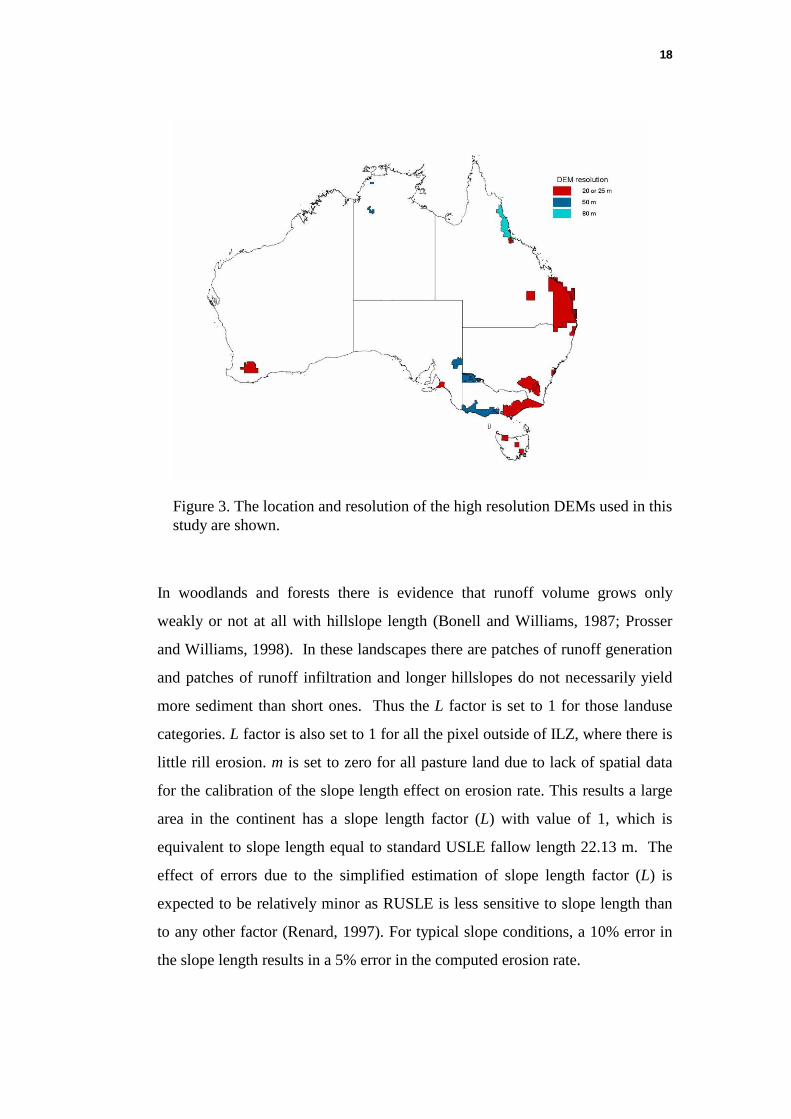
Hillslope length and mean slope were measured directly from available high

resolution DEMs. The hillslope length measurement technique examines the

landscape over a range of scales and identifies the average distance from ridges

to valleys. This analysis is repeated at regular intervals across the DEM,

producing a regular grid of hillslope length values. Mean slope was computed as

the mean slope value over a 250 m radius circular window. The DEMs used in

this analysis cover a range of topographies, geologies and climatic zones in WA,

NT, northern and southern Queensland, the western slopes of NSW, coastal

NSW, southern Victoria and north-western, central and south-eastern Tasmania.

Some of the DEMs were derived from contour and streamline data while others

were derived from data obtained during airborne geophysical surveys.

Resolutions ranged from 20 to 80 m. Figure 3 shows the location and resolution

of these high resolution DEMs used in this study.

Statistical predictive models for hillslope length and mean slope were

constructed using the Cubist data mining tool (decision rules based upon

piecewise linear regression, Quinlan, 1993) based on variables available for the

Australian intensive landuse zone (ILZ). The predictive model was then used to

derive estimates of the slope length and steepness across the entire study area,

using geology, soil class and several climatic and topographic attributes as

predictive variables. Details of estimating hillslope length and slope can be

found in a forthcoming technical report.

18

In woodlands and forests there is evidence that runoff volume grows only

weakly or not at all with hillslope length (Bonell and Williams, 1987; Prosser

and Williams, 1998). In these landscapes there are patches of runoff generation

and patches of runoff infiltration and longer hillslopes do not necessarily yield

more sediment than short ones. Thus the L factor is set to 1 for those landuse

categories. L factor is also set to 1 for all the pixel outside of ILZ, where there is

little rill erosion. m is set to zero for all pasture land due to lack of spatial data

for the calibration of the slope length effect on erosion rate. This results a large

area in the continent has a slope length factor (L) with value of 1, which is

equivalent to slope length equal to standard USLE fallow length 22.13 m. The

effect of errors due to the simplified estimation of slope length factor (L) is

expected to be relatively minor as RUSLE is less sensitive to slope length than

to any other factor (Renard, 1997). For typical slope conditions, a 10% error in

the slope length results in a 5% error in the computed erosion rate.

Figure 3. The location and resolution of the high resolution DEMs used in thisstudy are shown.

19

2.5 Supporting practice factor (P)

Supporting practice factor (P) accounts for the effects of contours, stripcropping

or terracing. It is defined as the ratio of soil loss with a specific supporting

practice to the corresponding soil loss with certain cultivation. Due to a lack of

spatial data on existing contour locations and tillage practices, it is assumed that

the values of P factor are 1 everywhere. Given this scenario, the estimated soil

loss rate reflects erosion potential under current conditions with no soil

conservation support practices.

3 RESULTS

3.1 Current Erosion

Figure 4 shows the predicted sheet and rill erosion, and Figure 5 shows the

monthly distributions. It is predicted that north part of the country has

considerably more erosion than the southern part of the country. This predicted

trend is consistent with measurements (Freebairn, 1982; Edwards, 1993).

It was found that about 4.8 × 109 tonnes of soil is moved annually on hillslopes

over the continent. It is 3-4 times smaller than previous estimation (Wasson et

al., 1996). Comparing with globe estimation (75 × 109 t yr-1, Pimentel et al.,

1995), it is predicted that Australia contributes 6.4% of globe soil erosion from

5% of the world land area. The average soil erosion is 6.3 t ha-1 yr-1. If we

denote that a pixel with soil loss rate below 0.5 t ha-1 yr-1 as low erosion, larger

than 10 t ha-1 yr-1 as high erosion, and in between as medium, it is estimated that

about 23% of the continent experiences low erosion, 16% faces high erosion and

61% of the continent experiences medium hillslope erosion. Overall, 25% of the

area is eroded at a rate greater than the continental average rate, showing the

potential to target erosion control to problem areas. Under any given rainfall

regime, the map shows that the reduction of protective ground cover increases

the risk of high soil losses.

Table 4 divides hillslope erosion into land use classes. In general, agricultural

lands have higher erosion rate compared with forest, but not necessarily more

Figure 4: Prediction of annual hillslope erosion hazard for the Australia continent.

Jan

May

Sep

Feb

Jun

Oct

Mar

Jul

Nov

Apr

Aug

Dec

Figure 5. Predicted monthly soil erosion rate patterns for the Australian continent.

20

erodible than native pasture lands. The predicted average erosion rates for

cereals are relatively low because they are often located in floodplains where the

slope is low. However, the rates are higher compared with surrounding non-

cropping area with similar climatic, soil and topographic conditions. This

confirms that land use and management practices have a major impact on soil

erosion. However, as our prediction is more or less based on the worst scenario

assumption for cropping land, the predicted rate for those lands could be higher

than the actual rate. The maps also identify areas of high soil erosion potential

within some of the National Parks in the tropics, but these are the natural

conditions in steep lands experiencing high intensity rainfall, and do not

represent elevated soil erosion rates.

Total soil loss is dominated by the pastoral industries, including grazed

woodlands, because of the vast areas that these land uses occupy. Thus the

sediment loads of large regional catchments such as the Burdekin and Fitzroy

catchments of Queensland will be dominated by sediment derived from pastoral

land. Cropping land of high erosion hazard is more restricted in extent but can

cause local problems as indicated by the high soil loss rates, and will be

Table 4: Soil Loss from land use categories.

Landuse Description Approx. Total area Total Erosion Average Erosion Rate Rate of acceleration

(km2) (t yr-1) (t ha-1 yr-1) Since EuropeanSettlement

Closed Forest 25,116 2,772,706 1.10 1.1

Open Forest 285,796 9,896,968 0.35 1.0

Woodland (unmanaged lands) 2,179,326 1,102,649,750 5.06 1.2

Commercial native forest production 157,460 5,864,068 0.37 1.1

National Parks 183,303 188,824,306 10.30 1.1

Cereals excluding rice 182,936 39,517,812 2.16 10.3

Legumes 22,568 795,556 0.35 3.2

Oilseeds 6,242 2,390,087 3.83 9.5

Rice 1,573 115,250 0.73 5.9

Cotton 4,053 2,784,581 6.87 11.3

Sugar Cane 4,736 18,694,681 39.47 56.8

Other agricultural landuse 2,138 2,402,811 11.24 33.6

Improved Pastures 200,295 46,307,300 2.31 5.1

Residual/Native Pastures 4,257,824 3,388,486,244 7.96 1.9

21

significant in relatively small catchments dominated by intensive land use. The

relatively high average erosion rates predicted for national parks is primarily due

to most national parks being located on north part of the country, where the

rainfall intensity is high, or in the arid inland, where the cover is low.

Figure 6 shows the monthly distribution of total soil loss. It is found that over

90% of the erosion occurs in the summer period (from November to April). This

summer dominant erosion pattern is clearly shown in Figure 5 especially for

tropical Australia, which is mainly caused by intensive summer monsoon

rainfall. However, the high erosion zone detected within the east part of Murray-

Darling Basin, is one of weaker summer dominance.

3.2 Prediction Evaluation of Current Hillslope Erosion

Researchers have undertaken a wide range of hillslope erosion plot

measurements in the past. The measurements methods include USLE plots

(Edwards, 1987), farm dam sediment survey (Neil and Fogarty, 1991; Throne,

1997), Caesium-137 (Loughran and Elliot, 1996) and sediment yield from small

catchment (Prove, 1991; Freebairn and Wockner, 1984). Figure 7 shows the

comparison between the predicted and measured hillslope erosion for the

-

2

4

6

8

10

12

14

Jan Feb Mar Apr May Jun Jul Aug Sep Oct Nov Dec

Monthly Total Erosion( 108 t yr-1 )

Figure 6. Monthly distribution of total soil loss estimated for Australia.

22

location where the measurements were undertaken. The comparison was made

by taking the 5%, mean and 95% (approximately) for both measurements and

predicted values for given landuse and locations. There are 103 points shown in

the Figure 7. Because it is often the case that latitudes and longitudes of the

nearest towns were given rather than the precise location of the measurements,

the predicted values shown in Figure 7 were calculated by taking 5%, average

and 95% for the given landuse near the town. The radius used for the average is

within the range from 1 km to 50 km according to individual literature. In some

cases, additional information, such as slope percentage is used for better

targeting the measurement location. Figure 7 shows, in most cases, that the

differences between prediction and measurements are within a factor of 10,

which is comparable to the range of measurements for the same location. The

linear correlation coefficient (Peason’s r) between measured and modelled mean

erosion rate is 0.815. No significant bias was obtained in the data. Given the

wide range of measurements we used for comparison, the quality of our input

data, and the scale of the analysis, we conclude that the results are encouraging.

We also found that it is often the case that our predicted values are smaller than

0.001

0.01

0.1

1

10

100

1000

0.001 0.01 0.1 1 10 100 1000

Measured Erosion Rate (t/ha/yr)

Pre

dic

ted

Ero

sio

nR

ate

(t/h

a/yr

)

Figure 7. The comparison between predicted and measured erosion ratesshowing the 5% (lower & left bars), mean (squares) and 95% (upper & rightbars) for both measurements and prediction with 103 observations. The 1:1line is shown.

23

Caesium-137, but larger than farm dam sedimentation or sediment yield

measurement. This is because the Caesium-137 accounts for all types of erosion,

including mass movement and wind erosion. On the other hand, farm dam

sedimentation and sediment yield should be smaller than hillslope erosion

because of deposition. The prediction matches USLE plots measurements

(Edwards, 1987) better, especially for cropping land, simply because the model

is initially calibrated from those data.

3.3 Erosion Rate between Current and Pre-European Settlement

To understand the impact of landuse and management practises on hillsope

erosion more, the predicted hillslope erosion needs to be put in the context of

erosion under natural vegetation cover. We predicted natural erosion using the

same procedure, with a cover factor for native vegetation and keeping the other

factors as for the present day.

We conducted a simple modelling framework to predict pre-European

settlement (undisturbed) USLE cover factor (C). Under this framework, we

assume that under certain similar climatic, geological and soil conditions, the

natural vegetation remains similar in terms of vegetation cover effect on erosion.

As only 3% of the continent areas are used as permanent cropping, we also

assume that the climate and geology do not change since European settlement.

Namely, landuse changes have relatively larger impact on cover management

factor but limited impact on climate. In each zone there are areas of reserve

where native vegetation cover is retained and for which the USLE C factor was

determined from remote sensing data for the assessment of current erosion rate.

By only sampling the pixel with limited human disturbance, such as National

Parks, Natural Forest and Crowned Aboriginal Conservation Land from the

NLWRA/BRS landuse map, statistical models were built relating cover and

management factor C to other climatic, geological and soil attributes using the

decision tree model Cubist. Figure 8 shows the comparison between samples of

C values extracted from the current C map and modelled C values for those

natural landuse pixels. The model was applied to the ILZ only because of the

minor disturbance and low input data quality in the areas outside of the ILZ. The

24

minimum value of predicted C and current C factor is used to get pre-European

settlement cover management factor with an underlying assumption that the

current C factor is always larger than native vegetation cover factor. The

maximum C value for natural vegetation cover is set to 0.45 as it is often

observed for the natural non-disturbed bare soil condition (RUSLE, Renard, et

al., 1997). Assuming L factor and P factor equal to 1 everywhere and other

factors unchanged, a map of pre-European hillslope erosion was calculated by

the same USLE equation Y = R K L S C P.

The acceleration of current mean annual soil loss above natural rates was

predicted as the ratio of current to pre-European hillslope erosion rates. The

ratio map (Figure 9) highlights those cropping lands and grazing lands where the

acceleration of erosion is high. It shows that erosion rate increased considerably

in the cropping areas, such as the Darling Downs, Colac in Victoria, wheat belt

of Western Australia, and Hunter Valley. It also shows erosion rate increases in

the areas experiencing intensive grazing land clearance after settlement. Those

areas include central and upper Burdekin (along the Burdekin River), Fitzroy

catchment and most eastern part of Murray-Darling Basin. Also shown in the

Figure 8. Comparison between actual cover and management factor C valuesand modelled C using Cubist. The line of best fit is shown.

36

Figure 9. Map shows the acceleration of hillslope erosion since European settlement. It is modelled by the ratio betweencurrent and pre-European settlement hillslope erosion rate. Negligible (ratio 0 – 1.5), Low (ratio 1.5 – 3), Moderately low(ratio 3 –5), Moderate (ratio 5–10), High (ratio 10 –25), Very High ( ratio > 25).

25

last column of Table 4, the predicted rates of acceleration of erosion since

European settlement are considerably higher for agricultural landuse groups

compared with other less disturbed landuse groups.

4 DISCUSSIONS AND CONCLUSIONS

Based on recently available topographic, rainfall, soil, landuse and time series

analysis of remotely sensed data, a nationwide prediction of hillslope erosion

has been developed. This study applied the USLE model on a monthly averaged

basis, calculating appropriate erosivity and cover factors for each month, to

represent the erosive potential of rainfall and runoff for each temporally distinct

period. The slope steepness factor is better handled by topographic scaling using

high resolution DEMs.

The broad predicted hillslope erosion patterns are consistent with a qualitative

analysis of plot data gathered from literature (Edwards, 1993). It is predicted

that hillslope erosion increases from south to north, which is mainly determined

by continental scale rainfall intensity pattern. Temporally, the erosion rate is

higher in summer for most of the continent, especially for the tropics, which also

follows the large scale climatic trend. Erosion rate is high for the area with steep

gradients. Regions such as Tasmania and SW Western Australia are predicted to

have low soil erosion rates, largely a result of low rainfall intensity at times of

low cover. Most of the predicted patterns are supported by the available field

data (Edwards, 1993; Throne, 1997).

The acceleration of erosion is studied by modelling the ratio between current

and pre-settlement hillslope erosion rate. The results show that although the

current erosion rates of cropping lands are not high compared with some landuse

groups, acceleration of erosion is high when it was put in context of erosion

under natural vegetation cover for the same location. It provides essential

information for the assessment of landuse impact in terms of possible

environmental degradation and pollution of both land and water resources.

26

The amount of gross erosion needs to be adjusted to account for rock cover. The

full erosion potential may not realised for some of the areas predicted as highly

erodible (such as upper Queensland and Northern Australia) because of the high

percentage of rock cover and shallow soil depth.

This study is aimed to provide broad scale (first order) nationwide erosion

estimation at a reconnaissance level. It could be useful for the purposes:

1. Identifying crucial catchments or sub-area appropriate for more detailed soil

erosion investigation;

2. Indicating the environmental health and agricultural Productivity and

sustainability at regional scale;

3. Providing sediment sources for modelling sediment transport in the river

system; and

4. Assessing the relative impact of landuse management on soil erosion.

It is not encouraged to use the results from this study for the estimation of soil

erosion rate at a fine scale, such as a specific paddock. Readers are reminded

that the vegetation covers were estimated using 8km resolution remotely sensed

data. The heterogeneous of cover can cause a great amount of variation in soil

erosion rate at a resolution smaller than 8km. Similar reason can be applied for

other factors.

Better prediction could be achieved by bringing in more information. For

example, prediction for cropping land can be improved by specifying tillage

types, crop rotation, contour cultivation and bank management. For pasture

lands, the erosion rate can be better predicted by giving grazing pressure for the

location. For forests, providing density of roads and logging frequency can

improve the prediction. However, more input data do not always guarantee

better prediction. Low quality inputs may introduce more errors and make the

overall prediction worse off. Therefore, it is important to check the input data

quality and its suitability before using them.

27

5 ACKNOWLEDGEMENTS

The research was supported by the National Land and Water Resource Audit

(NLWRA), Australia. The Queensland Department of Natural Resources is

acknowledged for permitting use of the interpolated daily rainfall data. We are

grateful for CSIRO Earth Observation Centre for offering the PAL GAC

AVHRR NDVI time series. Thanks to Dr. Tim McVicar for commenting on the

a draft of the manuscript and suggestions for using remote sensing data, Dr.

Damian Barret for processing the NDVI times series, and Dr. Mike Raupach for

helpful discussions. Dr. Janelle Stevenson is thanked for collecting plot

measurements data shown in Figure 7. Thanks to Dr. Elisabeth Bui for offering

advice of ASRIS soil attribute data sets. Thanks also to all the individuals who

are involved and worked hard in the NLWRA Theme 5.4 project. Heinz

Buettikofer helped with the layout and publishing on the Internet.

28

6 REFERENCES

Bonell, M. and Williams, J., (1987). Infiltration and redistribution of overlandflow and sediment on a low relief landscape of semi-arid, tropicalQueensland. IAHS Publication, 167: 199-211.

Bureau of Meteorology (1989). Climate of Australia. AGPS Press, Canberra.

Choudhury, B. (1989). Estimating evaporation and carbon assimilation usinginfrared temperature data: Vistas in modeling. In (Ed. Asrar, G.):Theory and Applications of Optical Remote Sensing, 628-690, JohnWiley and Sons, New York.

Cleveland, R.B., Cleveland, W.S., McRae, J.E., and Terpenning, I. (1990).STL: A Seasonal-Trend Decomposition Procedure Based on Loess(with Discussion). Journal of Official Statistics, 6:3-73.

DeFries, R.S., and Townshend, J.R.G. (1994). NDVI derived land coverclassification at global scales. International Journal of Remote Sensing,15: 3567-3586.

Edwards. K. (1987). Runoff and soil loss studies in New South Wales.Technical Handbook No. 10, Soil Conservation Service of NSW,Sydney, NSW.

Edwards, K. (1993). Soil erosion and conservation in Australia. In: World soilerosion and conservation, Ed: Pimentel, D., Cambridge, 147-169.

Freebairn, D.M. (1982). Soil erosion in perspective, In: Div. Land Util. Tech.News, Qld Dept Primary Ind., Brisbane, Australia, 6: 12-15.

Freebairn, D.M. and Wockner, G.H. (1986). A study of soil erosion onvertisols of the eastern Darling Downs, Queensland. 1. Effect of surfaceconditions on soil movement within contour bays. Australian Journalof Soil Research, 24: 135-58.

James, M.E. and Kalluri, S.N.V. (1994). The Pathfinder AVHRR land data set:an improved coarse resolution data set for terrestrial monitoring,International Journal of Remote Sensing, 15: 3347-3364.

Jeffrey, S.J., Carter, J.O., Moodie, K.B. and Beswick, A.R. (2001). Usingspatial interpolation to construct a comprehensive archive of Australianclimate data. Submitted to Journal of Hydrology.

29

Loch, R.J. and Rosewell, C.J. (1992). Laboratory methods for measurement ofsoil erodibility (K factors) for the Universial Soil Loss Equation.Australian Journal of Soil Research, 30: 233-48.

Loch, R. J., B. K. Slater, B. K. and Devoil, C. (1998). Soil erodibility (Km)values for some Australian soils. Australian Journal of Soil Research,36: 1045-55.

Loughran, R.J. and Elliott, G.L. (1996). Rates of soil erosion in Australiadetermined by the caesium-137 technique: a national reconnaissancesurvey. In: Erosion and Sediment Yield: Global and RegionalPerspectives. IAHS Publication. 236: 275-282.

Lovell, J.L. and Graetz, R.D. (2000). Filtering Pathfinder AVHRR Land NDVIdata for Australia. CSIRO Earth Observation Centre Internal Report.

McCool, D.K., Foster, G.R., Mutchler, C.K., and Meyer, L.D. (1989). Revisedslope length factor in the Universal Soil Loss Equation. Transactions ofthe American Society of Agricultural Engineers, 32: 1571-1576.

McFarlane, D.J., Davies, R.J., and Westcott, T., (1986). Fainfall erosivity inWestern Australia. Hydrology and Water Resources Symposium.Institution of Engineers, Australia National Conference Publication No.86/13, 350-4.

McIsaac, G.F., Mitchell, J.K. and Hirschi, M.C. (1987). Slope steepness effectson soil loss from disturbed lands, Transactions American. Society ofAgricultural Engineers, 30: 1005-1013.

McIvor, J.G., Williams, J. and Gardener, C.J. (1995). Pasture managementinfluences runoff and soil movement in the semi-arid tropics.Australian Journal of Experimental Agriculture, 35: 55-65.

McKenzie, N.J., Jacquier, D.W. Ashton, L.J. and Cresswell, H.P. (2000),Estimation of soil properties using the Atlas of Australian Soils.CSIRO Land and Water, Technical Report 11/00.

McVicar, T.R., Walker, J., Jupp, D.L.B., Pierce, L.L., Byrne, G.T. andDallwitz, R. (1996a). Relating AVHRR vegetation indices to in situleaf area index. CSIRO Division of Water Resources, Canberra, ACT.

McVicar, T.R., Jupp, D.L.B., and Williams, N.A. (1996b). Relating AVHRRvegetation indices to LANDSAT TM leaf area index estimates. CSIRODivision of Water Resources, Canberra, ACT.

Neil, D.T., and Fogarty P (1991). Land use and sediment yield on the southerntablelands of New South Wales. Australian Journal of Soil and WaterConsevation, 4: 33-39.

30

Northcote, K.H. with Beckmann G.G, Bettenay E., Churchward H.M., vanDijk D.C., Dimmock G.M., Hubble G.D., Isbell R.F., McArthur W.M.,Murtha G.G., Nicolls K.D., Paton T.R., Thompson C.H., Webb A. A.and Wright M. J. (1960-68). Atlas of Australian Soils, Sheets 1 to 10,with explanatory data. CSIRO and Melbourne University Press:Melbourne.

Pimentel, D., Harvey, C., Resosudarmo, P., Sinclair, K., Kurz, D., McNair, M.,Crist, S., Shpritz, L., Fitton, L., Saffouri, R. and Blair, R. (1995).Environmental and economic costs of soil erosion and conservationbenefits. Science, 267: 1117-1123.

Prosser, I.P. and Williams, L. (1998). The impact of wildfire on runoff anderosion in native Eucalyptus forest. Hydrological Processes, 12: 251-265.

Prove, B. C. (1984). Soil erosion and conservation in the sugar-canelands ofthe wet tropical coast. Erosion Research Newsletter, 10: 6-7.

Quinlan, J.R. (1993) C4.5: Programs for Machine Learning, MorganKaufmann Publishers, San Mateo, California. . For further informationsee: http://www.rulequest.com.

Renard, K.G., Foster, G.A., Weesies, D.K., McCool, D.K., and Yoder, D.C.(1997). Predicting soil erosion by water: A guide to conservationplanning with the Revised Universal Soil Loss Equation. AgricultureHandbook 703, United States Department of Agriculture, WashingtonDC.

Roderick M.L., Noble I.R., Cridland S.W. (1999). Estimating woody andherbaceous vegetation cover from time series satellite observations.Global Ecology and Biogeography, 8: 501-508.

Rosenthal K.M. and White B.J. (1980). Distribution of a rainfall erosion indexin Queensland. Report 80/8, Department of Primary Industries,Queensland.

Rosewell, C.J. (1993). SOILOSS - A program to assist in the selection ofmanagement practices to reduce erosion. Technical Handbook No. 11(2nd edition) Soil Conservation Service of NSW, Sydney.

Rosewell, C.J. (1997). Potential source of sediments and nutrients: Sheet andrill erosion and phosphorus sources. Australia: State of theEnvironment Technical Paper Series (Inland Waters), Department ofthe Environment, Sport and Territories, Canberra.

Scanlan, J.C., Pressland, A.J. and Myles, D.J. (1996). Run-off and soilmovement on mid-slopes in north-east Queensland grazed areas.Rangeland Journal, 18: 33-46.

31

Throne J. (1997). Estimation of sediment yields from small agriculturalcatchments within Oyster Harbour, Albany. BSc Hons. Thesis,University of Western Australia (Unpublished).

Wasson, R.J., Olive, L.J. and Rosewell, C.J. (1996). Rates of erosion andsediment transport in Australia. IAHS Publication, 236: 139 – 148.

Wischmeier W.H., Johnson, C. B. and Cross, B. V. (1971). A soil erodibilitynomograph for farmland and construction sites. Journal of Soil andWater Conservation, 26: 189-183.

Wischmeier, W. H. and Smith, D. D. (1978). Predicting rainfall erosion losses:A guide to conservation planning. US Department of Agriculture.Agriculture Handbook No. 537. (US Government Printing Office:Washington, DC).

Yu, B. and Rosewell, C. J. (1996a). An assessment of a daily rainfall erosivitymodel for New South Wales. Australian Journal of Soil Research, 34:139-52.

Yu, B. and Rosewell, C. J. (1996b). A robust estimator of the R-factor for theUniversal Soil Loss Equation. Transactions American Society ofAgricultural Engineers, 39, 559-61.

Yu, B. (1998). Rainfall erosivity and its estimation for Australia’s tropics.Australian Journal of Soil Research, 36, 143-165.