Prediction of Icing Effects on the Dynamic Response of ... · Prediction of Icing Effects on the...
11
Prediction of Icing Effects on the Dynamic Response of Light Airplanes Amanda Lampton ∗ and John Valasek † Texas A&M University, College Station, Texas 77843-3141 DOI: 10.2514/1.25687 The accumulation of ice on an airplane in flight is one of the leading contributing factors to general aviation accidents. To date, only relatively sophisticated methods based on detailed empirical data and flight data exist for its analysis. This paper develops a methodology and simulation tool for preliminary safety and performance evaluations of airplane dynamic response and climb performance in icing conditions. The important aspect of dynamic response sensitivity to pilot control input with the autopilot disengaged is also highlighted. Using only basic mass properties, configuration, propulsion data, and known icing data from a similar configuration, icing effects are applied to the dynamics of a non-real-time, six degree-of-freedom simulation model of a different, but similar, light airplane. Besides evaluating various levels of icing severity, the paper addresses distributed icing which consists of wing alone, horizontal tail alone, and unequal distributions of combined wing and horizontal tail icing. Results presented in the paper for a series of simulated climb maneuvers with various levels and distributions of ice accretion show that the methodology captures the basic effects of ice accretion on pitch response and climb performance, and the sensitivity of the dynamic response to pilot control inputs. Nomenclature A = plant matrix B = control distribution matrix C = output matrix C A = arbitrary stability and control derivative C A iced = arbitrary stability and control derivative with icing effects C D = airplane drag coefficient C L = airplane lift coefficient C m = airplane pitching moment coefficient C Z = stability z-axis coefficient Presented as Paper 6219 at the Atmospheric Flight Mechanics, San Francisco, CA, 15–18 August 2005; received 16 June 2006; accepted for publication 27 November 2006. Copyright © 2007 by Amanda Lampton and John Valasek. Published by the American Institute of Aeronautics and Astronautics, Inc., with permission. Copies of this paper may be made for personal or internal use, on condition that the copier pay the $10.00 per-copy fee to the Copyright Clearance Center, Inc., 222 Rosewood Drive, Danvers, MA 01923; include the code 0731-5090/07 $10.00 in correspondence with the CCC. ∗ Graduate Research Assistant, Flight Simulation Laboratory, Aerospace Engineering Department, 3141 TAMU; [email protected]. Student Member AIAA. † Associate Professor and Director, Flight Simulation Laboratory, Aerospace Engineering Department, 3141 TAMU; [email protected]. Associate Fellow AIAA. Amanda Lampton earned the B.S. Cum Laude with Distinction (2004) and M.S. in aerospace engineering (2006) from Texas A&M University as a participant in the Engineering Scholars Program. She is a recipient of the National Science Foundation Graduate Fellowship, the Zonta International Foundation Amelia Earhart Fellowship, the Armed Forces Communications and Electronics Assoc. (AFCEA) General John A. Wickham Scholarship, and the United States Academic Decathlon Scholarship. She is a member of Sigma Gamma Tau, the aerospace engineering honor society, Phi Kappa Phi, Tau Beta Pi, the National Society of Collegiate Scholars, Phi Eta Sigma, the Society of Women Engineers, and the Texas A&M University Sky Diving Club, and Cycling Team. In 2005, she interned at Eclipse Aviation, performing parameter identification and aerodynamic data reduction with the Eclipse 500 flight test group. She is currently a graduate research assistant and Ph.D. candidate in the Flight Simulation Laboratory at Texas A&M University, researching ice accretion effects on aircraft dynamics and stability, and artificial intelligence techniques for control of morphing air vehicles. She is a member of AIAA. John Valasek earned the B.S. degree in aerospace engineering from California State Polytechnic University, Pomona in 1986, and the M.S. degree with honors, and the Ph.D. in aerospace engineering from the University of Kansas, in 1991 and 1995, respectively. He was a flight control engineer for the Northrop Corporation, Aircraft Division from 1985 to 1988, where he worked in the Flight Controls Research Group, and on the AGM-137 Tri- Services Standoff Attack Missile (TSSAM) program. He previously held an academic appointment at Western Michigan University (1995-1997), was a summer faculty researcher at NASA Langley Research Center (1996), and an Air Force Office of Scientific Research (AFOSR) summer faculty research fellow at the Air Force Research Laboratory (1997). Since then, he has been with Texas A&M University, where he is Associate Professor of aerospace engineering, and Director of the Flight Simulation Laboratory. He teaches courses on digital control, nonlinear systems, flight mechanics, aircraft design, and coteaches a short course on digital flight control for the University of Kansas Division of Continuing Education. Current research interests include control of morphing air and space vehicles, multi-agent systems, intelligent autonomous control, vision-based navigation systems, and fault-tolerant adaptive control. He is an Associate Fellow of AIAA, past Chairman and current member of the Atmospheric Flight Mechanics Technical Committee, and current member of the Intelligent Systems, Guidance Navigation, and Control Technical Committees. JOURNAL OF GUIDANCE,CONTROL, AND DYNAMICS Vol. 30, No. 3, May–June 2007 722
Transcript of Prediction of Icing Effects on the Dynamic Response of ... · Prediction of Icing Effects on the...
Prediction of Icing Effects on the Dynamic Responseof Light Airplanes
Amanda Lampton∗ and John Valasek†
Texas A&M University, College Station, Texas 77843-3141
DOI: 10.2514/1.25687
The accumulation of ice on an airplane in flight is one of the leading contributing factors to general aviation
accidents. To date, only relatively sophisticated methods based on detailed empirical data and flight data exist for its
analysis. This paper develops amethodology and simulation tool for preliminary safety andperformance evaluations
of airplane dynamic response and climb performance in icing conditions. The important aspect of dynamic response
sensitivity to pilot control input with the autopilot disengaged is also highlighted. Using only basic mass properties,
configuration, propulsion data, and known icing data from a similar configuration, icing effects are applied to the
dynamics of a non-real-time, six degree-of-freedom simulation model of a different, but similar, light airplane.
Besides evaluating various levels of icing severity, the paper addresses distributed icing which consists of wing alone,
horizontal tail alone, and unequal distributions of combined wing and horizontal tail icing. Results presented in the
paper for a series of simulated climb maneuvers with various levels and distributions of ice accretion show that the
methodology captures the basic effects of ice accretion on pitch response and climb performance, and the sensitivity
of the dynamic response to pilot control inputs.
Nomenclature
A = plant matrixB = control distribution matrixC = output matrixC�A� = arbitrary stability and control derivative
C�A�iced = arbitrary stability and control derivative with icingeffects
CD = airplane drag coefficientCL = airplane lift coefficientCm = airplane pitching moment coefficientCZ = stability z-axis coefficient
Presented as Paper 6219 at the Atmospheric Flight Mechanics, San Francisco, CA, 15–18 August 2005; received 16 June 2006; accepted for publication 27November 2006. Copyright © 2007 by Amanda Lampton and John Valasek. Published by the American Institute of Aeronautics and Astronautics, Inc., withpermission. Copies of this paper may be made for personal or internal use, on condition that the copier pay the $10.00 per-copy fee to the Copyright ClearanceCenter, Inc., 222 Rosewood Drive, Danvers, MA 01923; include the code 0731-5090/07 $10.00 in correspondence with the CCC.
∗Graduate ResearchAssistant, Flight Simulation Laboratory, Aerospace EngineeringDepartment, 3141 TAMU; [email protected]. StudentMemberAIAA.†Associate Professor and Director, Flight Simulation Laboratory, Aerospace Engineering Department, 3141 TAMU; [email protected]. Associate Fellow
AIAA.
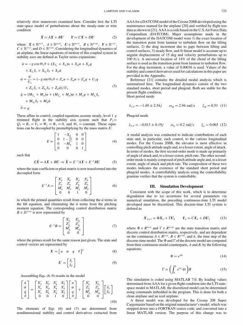
Amanda Lampton earned the B.S. Cum Laude with Distinction (2004) and M.S. in aerospace engineering (2006)
fromTexas A&MUniversity as a participant in the Engineering Scholars Program. She is a recipient of the National
Science Foundation Graduate Fellowship, the Zonta International Foundation Amelia Earhart Fellowship, the
Armed Forces Communications and Electronics Assoc. (AFCEA) General John A. Wickham Scholarship, and the
United States Academic Decathlon Scholarship. She is a member of Sigma Gamma Tau, the aerospace engineering
honor society, Phi Kappa Phi, Tau Beta Pi, the National Society of Collegiate Scholars, Phi Eta Sigma, the Society of
Women Engineers, and the Texas A&M University Sky Diving Club, and Cycling Team. In 2005, she interned at
Eclipse Aviation, performing parameter identification and aerodynamic data reduction with the Eclipse 500 flight
test group. She is currently a graduate research assistant and Ph.D. candidate in the Flight Simulation Laboratory at
TexasA&MUniversity, researching ice accretion effects on aircraft dynamics and stability, and artificial intelligence
techniques for control of morphing air vehicles. She is a member of AIAA.
John Valasek earned the B.S. degree in aerospace engineering from California State Polytechnic University,
Pomona in 1986, and the M.S. degree with honors, and the Ph.D. in aerospace engineering from the University of
Kansas, in 1991 and 1995, respectively. He was a flight control engineer for the Northrop Corporation, Aircraft
Division from 1985 to 1988, where he worked in the Flight Controls Research Group, and on the AGM-137 Tri-
Services Standoff Attack Missile (TSSAM) program. He previously held an academic appointment at Western
Michigan University (1995-1997), was a summer faculty researcher at NASA Langley Research Center (1996), and
an Air Force Office of Scientific Research (AFOSR) summer faculty research fellow at the Air Force Research
Laboratory (1997). Since then, he has beenwithTexasA&MUniversity, where he isAssociate Professor of aerospace
engineering, and Director of the Flight Simulation Laboratory. He teaches courses on digital control, nonlinear
systems, flight mechanics, aircraft design, and coteaches a short course on digital flight control for the University of
Kansas Division of Continuing Education. Current research interests include control of morphing air and space
vehicles, multi-agent systems, intelligent autonomous control, vision-based navigation systems, and fault-tolerant
adaptive control. He is an Associate Fellow of AIAA, past Chairman and current member of the Atmospheric Flight
Mechanics Technical Committee, and currentmember of the Intelligent Systems, GuidanceNavigation, andControl
Technical Committees.
JOURNAL OF GUIDANCE, CONTROL, AND DYNAMICS
Vol. 30, No. 3, May–June 2007
722

�c = mean geometric chordD = carry through matrixfice = icing factorg = gravitational accelerationh = integration step sizeIyy = airplane moment of inertia about y axisi = index, imaginary componentj = imaginary componentk0CA = coefficient icing factor constantL = roll angular accelerationM = pitch angular acceleration; modal matrixN = yaw angular accelerationnframes = number of time stepsP = airplane body-axis roll ratep = perturbed airplane body-axis roll rateQ = airplane body-axis pitch rateq = perturbed airplane body-axis pitch rate_q = airplane body-axis pitch acceleration�q = dynamic pressureR = airplane body-axis yaw rater = perturbed airplane body-axis yaw rateS = wing areat = timeU = airplane velocity in the body-axis x directionU = control input vectoru = stability axis airplane velocity in the x direction_u = incremental change in the stability axis airplane
velocity in the x directionV = airplane velocity in the body-axis y directionW = airplane velocity in the body-axis z direction_w = incremental change in the stability axis airplane
velocity in the z directionX = linear acceleration in the body x-axis directionX = state vector_X = derivative of state vectorY = linear acceleration in the body y-axis directionY = output vectorZ = linear acceleration in the body z-axis direction� = angle of attack_� = incremental change in angle of attack� = discrete control distribution matrix� = control deflection angle� = damping ratio�ice = icing severity parameter�1 = airplane steady-state pitch attitude angle� = pitch attitude angle_� = incremental change in pitch attitude angle� = eigenvector� = modal vector� = time constant; dummy time variable� = airplane roll attitude angle; discrete plant matrix! = frequency
Subscripts
a = ailerond = Dutch roll modee = elevatorice = ice accretion effecticed = ice accretion effectk = index for discretized modelm = modalp = phugoid modeq = derivative with respect to airplane pitch rater = rudder; roll modes = spiral modesp = short period modeTu = derivative with respect to change in speed due to
thrustT� = derivative with respect to change in angle of attack
due to thrust
u = derivative with respect to stability x-axis airplanevelocity
� = derivative with respect to angle of attack_� = derivative with respect to incremental change in
angle of attack�e = derivative with respect to elevator deflection angle0 = derivative with respect to zero angle of attack; initial
condition1 = steady state; first mode2 = second mode
I. Introduction
I NCLEMENT weather accounted for an average of 19.6% ofenvironment-related, reported general aviation accidents
annually from 1998 to 2000 according to theNational TransportationSafety Board [1–3]. Of this annual percentage, icing conditionsaccounted for 2.9% of general aviation accidents in 1997, 2.4% in1998, 3.6% in 1999, and 2.7% in 2000, inwhich 36.4, 55.6, 46.2, and40.0% of those resulted in fatalities in 1997, 1998, 1999, and 2000,respectively [1–4]. Rime, glaze, and mixed ice along the leadingedge of lifting surfaces all have detrimental effects on airplaneperformance. Although anti-icing devices such as de-icing boots andheating strips help, ice accretions can still build up and affect theairplane adversely by increasing drag, decreasing airplane lift curveslope, and decreasing static longitudinal stability. Additionally,malfunctions of these anti-icing systems can result in ice buildup aftof the devices themselves, or ice buildup between the cycles of thede-icing systems. The type and severity of ice accretions is highlydependent on a number of factors. These include, but are not limitedto, the following: velocity of the airplane, exposure time,atmospheric air temperature, liquid water content, and medianvolumetric diameter.
The danger of a climbwith ice accretions on the airplane lays in thesusceptibility of the ice to cause a separation bubble (Fig. 1) [5]. Thisphenomenon is usually caused by a horn of ice disrupting the flow ofair over the airfoil and creating an adverse pressure gradient. Thisdisruption forms a separation bubble that reattaches furtherdownstream. However, increasing the elevator deflection angle alsoincreases the angle of attack, thus pushing the reattachment pointfarther downstream and increasing the size of the separation bubble.As the bubble increases in size, elevator effectiveness decreases andfull departure of the airplane becomes more likely. Bragg et al. havedeveloped an icing-effects model applicable to any individualperformance, stability, or control derivative affected by icing [6].The model is characterized by dependence on atmosphericconditions, susceptibility of an airplane to icing, and a givenderivative as seen in Eq. (1).
C�A�iced � �1� �icek0CA�C�A� (1)
This model is still being refined, withmany of the influencing factorsstill unknown [6]. The model was then integrated into a flightdynamics and control toolbox for MATLAB and Simulink [7],which produces results showing the possible changes of an airplane’sstability derivatives over time with icing effects.
The practicality of using an autopilot during icing conditions hasalso been studied. Sharma et al. has designed a pitch angle holdautopilot that considers ice accretion severity when processing the
Fig. 1 Schematic of upper surface separation bubble aft of leading-
edge ice accretion [5].
LAMPTON AND VALASEK 723

commanded pitch attitude angle; the goal being to maintain thestability of the airplane [8]. The commanded value for the pitchattitude angle is then modified based on an envelope protectionalgorithm that references flight test data of ice severity and wing stallangle of attack [8]. The purpose is to prevent the airplane fromreaching the icing-modified wing stall angle of attack, and pitchattitude response is investigated. Distributed levels and severities oficing between the wing and horizontal tail are not specificallyaddressed, and the iced airplane model and the autopilot areapplicable only to the DeHavilland Twin Otter [8]. Additionally, theimportant aspect of sensitivity of airplane response to pilot commandinputs in icing conditions with the autopilot disabled, which is theautopilot status recommended by the Federal Aviation Admin-istration (FAA) in these conditions, is not addressed.
The area of forensic engineering is also concerned with the effectice has on climb performance and aerodynamic degradation [9]. Theresearch described in [9] concerns the dangerous reduction in stallangle of attack and how climbing at high angles of attack couldapproach this reduced stall angle causing an unexpected wing stall.The nonlinear simulation incorporating the effects of ice accretionwas set up specifically for a jet trainer in an attempt to project thetrajectory of a crash caused by ice accretion [9].
Much other research in the area of the influence of ice regardsairfoil aerodynamics. Lee and Bragg explore the changes in airfoilsection lift, drag, and pitching moment with simulated ice shapes[10]. Intercycle ice accretions have a distinct effect on airfoilproperties as described in [11]. In this case, the buildup of icebetween pneumatic boot inflation and the possible ice ridge left justbehind where the boot meets the skin of the airfoil is analyzed [11].The resulting increase in drag, decrease in lift, and change in pitchingmoment is tabulated [11]. In general, the consensus appears to be thatthe aerodynamics of an airfoil is degraded by ice accretion such thatlift decreases, drag increases, stall angle of attack is reduced, andpitching moment is degraded [9–16].
Efforts have been made to develop icing protection systems,especially by Bragg et al. [17]. They propose a smart icing systembased on the ability to sense the effect of ice on aircraft performance,stability, and control. The system would enhance the level of safetyoffered by current icing avoidance and protection concepts [17]. TheSmart Icing System senses ice accretion through traditional icingsensors and uses modern system identification methods to estimateaircraft performance and control changes [18].
Airplane response due to pilot command inputs with the autopilotdisengaged is a critical safety issue, because the FAA recommendsthat the autopilot must be disengaged during flight in known icingconditions. The danger lies in a pilot attempting to command an icedairplane in the same way as a noniced airplane because overlyaggressive pilot command inputs (for the iced situation) can produceexcessive climb rates which can lead to stall, and/or overshoots andundershoots in commanded altitude. This is particularly critical forsituations in which the pilot is not even aware that the airplaneresponse and performance has been compromised by icing, and it hasnot been reported on in the open literature.
This paper details the development of a simplified method for theprediction of icing effects and pilot command effects on the dynamicresponse and climb performance of light airplanes, for which icingdata may not exist or might not be obtainable. The method permits arapid, first cut prediction and analysis of performance of icing effectsusing only basic, relatively easy to obtain or generate data as aprecursor to a highly detailed analysis using sophisticated and costlymodeling and analysis methods. It is equally applicable to eitherperformance prediction or accident reconstruction and has been usedfor both. The unique contributions of this paper to the literature arethreefold. It details a method to model and investigate airplanes forwhich icing data does not exist, or is not available in the openliterature. This is done using known icing data obtained from eitherflight data or wind-tunnel data or both, for airplanes of similar butdifferent configurations, using appropriate scaling and modification.It also considers the modeling and evaluation of unequallydistributed icing levels and icing severity between the wing, thehorizontal tail, and the full aircraft, in terms of dynamic response.
The metrics used are rate-of-climb and commanded altitude capturesconsisting of overshoots and undershoots. Finally, this paperinvestigates sensitivity to pilot command inputs during icingconditions in terms of dynamic response and climb performance,with the autopilot disengaged as per FAA recommendation. Theapproach developed here is used to construct a linear time invariant(LTI), six degree of freedom, non-real-time flight simulation codewhich has the capability to evaluate a variety of time-varying pilotinputs, such as singlets, doublets, and ramps, during icing conditions.The scope of this work is limited to the pitch axis, where the mostdetrimental icing effects are typically experienced.
The paper is organized as follows. First, a nonparametric linearmodel of a Cessna 208B Super Cargomaster (Fig. 2) is developed, inwhich stability and control derivatives are calculated using datacompendium (DATCOM) methods and the Advanced AircraftAnalysis (AAA) computer program [19]. Verification of themodel isaccomplished by comparing simulation data to published flight testdata. To ensure the fidelity of the model, a modal analysis wasconducted to examine the characteristics of the flight modes. Inaddition, a controllability analysis was conducted to check that thesystem was indeed linearly independent and controllable. Next, thestability derivatives calculated for eachflight condition of interest areused to construct multiple LTI state-space models. Various levels ofice accretion severity are then added to the clean airplane simulationbased on icing data gathered by NASA John H. Glenn ResearchCenter on the DeHavilland Twin Otter [6]. A series of simulationexamples are presented for climb maneuvers with varying amountsof ice accretion, together with an investigation of the dynamic effectof overcontrolling the airplane during a climb. Finally, a summaryand conclusions are presented.
II. State-Space Model Representation
To determine the response of an LTI system to an arbitrary inputsignal, it is transformed into a state-space representation of thesystem. The system analyzed in this paper is a continuous dynamiclinear system in the stability axis. Figure 3 shows the body-axissystems for reference. Time invariance of the model is assumedbecause the parameters in the model do not change quickly for the
Fig. 2 Cessna 208B Super Cargomaster external characteristics [21].
Fig. 3 Body-axis systems and aerodynamic angles.
724 LAMPTON AND VALASEK
relatively slow maneuvers examined here. Consider first the LTIstate-space model of perturbations about the steady-state or trimcondition
_X� AX� BU Y � CX�DU (2)
where X 2 Rn�1, A 2 Rn�n, U 2 Rm�1, B 2 Rn�m, Y 2 Rr�1,C 2 Rr�n, andD 2 Rr�m. Considering the longitudinal dynamics ofan airplane, the linear equations of motion of this coupled system instability axes are defined as Taylor series expansions:
_u��g cos�1�� �XTu � Xu�u� X��� Xqq� X�e�e � X�T �T � X _� _�
_�� _w
U1
� ��g sin�1�� Zuu� Z��� Zqq�U1q
� Z�e�e � Z�T �T � Z _� _��=U1
_q� �MTu�Mu�u� �MT�
�M����Mqq�M�e�e
�M�T�T �M _� _�
_�� q
(3)
These affine in control, coupled equations assume steady, level 1 gtrimmed flight in the stability axis system such that P1�Q1 � R1 � V1 �W1 ��1 � 0, and �1 � constant. These equa-tions can be decoupled by premultiplying by the mass matrix E:
E�
1 �X _� 0 0
0 1 � Z _�
U10 0
0 �M _� 1 0
0 0 0 1
2664
3775 (4)
such that
E _X� AX� BU) _X� E�1AX� E�1BU (5)
where the state coefficient or plantmatrix is now transformed into thedecoupled form
E�1A�
X0u X0� X0q X0�Z0u Z0� Z0q Z0�M0u M0� M0q M0�0 0 1 0
2664
3775 (6)
in which the primed quantities result from collecting the _� terms inthe lift equation, and eliminating the _� terms from the pitchingmoment equation. The corresponding control distribution matrixB 2 Rn�m is now represented by
E�1B�
X0�e X0�TZ0�e Z0�TM0�e M0�T0 0
2664
3775 (7)
where the primes result for the same reason just given. The state andcontrol vectors are represented by
X � u � q �� �
T (8)
U � �e�T
� �(9)
Assembling Eqs. (6–9) results in the model
_u_�_q_�
2664
3775�
X0u X0� X0q X0�X0u X0� X0q X0�X0u X0� X0q X0�0 0 1 0
2664
3775
u�q�
2664
3775�
X0�e X0�TZ0�e Z0�TM0�e M0�T0 0
2664
3775 �e
�T
� �
(10)
The elements of Eqs. (6) and (7) are determined fromnondimensional stability and control derivatives extracted from
AAA for aDATCOMmodel of theCessna 208Bdeveloped using themaintenance manual for the airplane [20] and verified by flight testdata as shown in [21].AAA is a code based on theU.S.Air ForceDataCompendium (DATCOM). Major assumptions made in thedevelopment of the DATCOM model were 1) the exact location ofthe transition point from laminar to turbulent flow on the liftingsurfaces, 2) the drag increment due to gaps between lifting andcontrol surfaces, 3) steady flow, and 4) linear model is accurate up toangular displacements of 15 deg and velocity perturbations up to100 ft=s. A universal location of 14% of the chord of the liftingsurface is used as the transition point from laminar to turbulent flow.For the drag increment, a value of 0.00036 is used. Values of thestability and control derivatives used for calculations in this paper areprovided in the Appendix.
Reference [21] contains the detailed modal analysis which issummarized here. The longitudinal dynamics consist of the twostandard modes, short period and phugoid. Both are stable for thepresent flight condition.Short period mode
1;2 ��1:49� 2:54j !sp � 2:94 rad=s �sp � 0:51 (11)
Phugoid mode
3;4 ��0:013� 0:19j !p � 0:2 rad=s �p � 0:065 (12)
A modal analysis was conducted to indicate contributions of eachstate and, in particular, each control, to the various longitudinalmodes. For the Cessna 208B, the elevator is most effective incontrolling pitch attitude angle and, to a lesser extent, angle of attack.In terms of modes, the first second-order mode is made up primarilyof angle of attack and, to a lesser extent, pitch rate. The other second-ordermode ismainly composed of pitch attitude angle and, to a lesserextent, angle of attack and pitch rate. The composition of these twomodes indicates the existence of the standard short period andphugoid modes. A controllability analysis using the controllabilitygramian verifies that the system is controllable.
III. Simulation Development
Consistent with the scope of this work, which is to determinedegradation due to ice accretions for several parameters vianumerical simulation, the preceding continuous-time LTI modeldeveloped must be discretized. This discrete-time LTI system isdefined as
X k�1 ��Xk � �Uk Yk � CXk �DUk (13)
where � 2 Rn�n and � 2 Rn�m are the state transition matrix anddiscrete control distribution matrix, respectively, and are dependenton the continuous A 2 Rn�n, B 2 Rn�m, and h, the time step of thediscrete-timemodel. The� and� of the discretemodel are computedfrom their continuous model counterparts, A andB, by the followingequations:
�� eAh (14)
���Z
h
0
eA� d�
�B (15)
The simulation is coded using MATLAB 7.0. By loading valuesdetermined fromAAA for a given flight condition into the LTI state-space model in MATLAB, the discretized model can be determinedusing commands imbedded in the program. This is done for both aclean airplane and an iced airplane.
A thrust model was developed for the Cessna 208 SuperCargomaster based on the original manufacturer’s model, which wasstripped down into a FORTRAN source code, and converted into alinear MATLAB version. The purpose of this change was to
LAMPTON AND VALASEK 725

streamline the simulation as a whole, allowing thrust data to beupdated every time step. This MATLAB-based thrust model wasimplemented and current data for the simulationwas obtained using aseries of table lookups in which the inputs are values such as currentairspeed, rate of climb, ambient temperature, pressure, density,current altitude, and dynamic pressure. In addition, the thrust modelis dependent on the prop control lever and power level position,which allows the throttle and therefore the thrust to be modifiedduring the simulation. An example of this feature is shown later inthis paper. The thrust model also accounts for corrections due tocabin heat, cabin temperature, and the status of the inertial separatorsystem (ISS) in an effort to make the model as accurate as possible.
The thrust model calculations begin with determining inlettemperature and pressure. Then it proceeds to calculate fuel flow andgas generator speeds based on the settings for the ISS, power leverangle, and power control lever. Additional corrections wereintroduced to take into account decreases in fuel flow and gasgenerator revolutions per minute losses due to the ISS, cabin heat,and high-powered climbs. Propeller revolutions per minute are thendetermined using the values already calculated. Finally, shafthorsepower, net propeller thrust, gross jet thrust, ram drag, propefficiency, airflow, and airplane thrust coefficient are calculatedwithcorrections for the ISS and cabin heat. These data are used todetermine the control derivatives due to thrust, as well as thrust anddrag due to thrust for each time step of the simulations.
IV. Modeling and Incorporation of Icing Effects
The extent towhich each stability and control derivative is affectedby ice accretions is based on previous studies, in particular thoseconcerning the flight dynamics of a DeHavilland Twin Otter [6,22].Twin Otter data were used because there is more icing data availableof the type needed for this research than for any other airplanereported in the open literature. In general, the effectiveness of CL,Cm,CD,CL� ,Cm� ,CD� ,CLq ,Cmq ,CL�e , andCm�e have been observed
to degrade between 5 and 35%. As ice builds up on the leading edgeof the wing and horizontal tail, the carefully engineered liftingsurfaces are compromised, thus they produce less lift. Also, the iceaccretion may develop horns that protrude into the airflow as well asincreasing surface roughness leading to an increase in drag. Theexact amount of degradation, whether it is an increase in lift, decreasein drag, or change in pitching moment, depends on both the airplaneconfiguration and the particular derivative in question. Thepercentage of degradation for each derivative is imbedded within theMATLAB program that dimensionalizes the values calculated byAAA. Each of these dimensionalized counterparts of the derivativesis multiplied by an icing factor causing the derivative in question tobecome less stable. For example, the modification for Cm� is
M�iced ��qS �c��1� fice��Cm�
Iyy(16)
such that static stability is reduced as Cm� decreases. In this case, anfice value of �0:099 is the degradation factor, meaning that Cm�becomes less stable by almost 10%, based on data from theDeHavilland Twin Otter [6]. For the numerical examples, thesedegradation factors are assumed to be the worst case scenario foricing on the Cessna 208B.
Equation (16) generalizes the terms first presented in Eq. (1). Forthe purposes of this research, fice represents the term �icek
0CA. The
actual parameterization of the terms �ice and k0CA
is beyond the scope
of this paper, but is being addressed by other researchers. Instead, ficefor each pertinent longitudinal derivative is calculated fromflight testdata of the DeHavilland Twin Otter in both clear and icingconditions, as detailed in [6]. Because comprehensive icing data arenot readily available for the Cessna 208B, applying icing dataobtained from the DeHavilland Twin Otter does not fully representwhat actually occurs in icing conditions. However, the simulateddynamic responses and performance are consistent with the limited
scope and objectives of this research. Values of fice are presented inTable 1.
To analyze how the flight dynamics and performance change withice accretion severity, additional factors are included in thecalculation of the iced derivatives to represent various levels ofseverity. For example, the nominal fice degradation factor for Cm� is�0:099, as stated before. For a totally iced condition, the worst casefor theCessna 208B isfice multiplied by 1.0. It is assumed that the 1.0is implicit in Eq. (16). Similarly, if only mild icing is of interest, thenfice may only be multiplied by 0.2, as shown in the followingequation
M�iced�
�qS �c�1� 0:2fice�Cm�Iyy
(17)
For the example shown, 0:2fice � 0:2��:099� � �0:0198, whichmeans that for “mild” iceCm� becomes less stable by about 2%. Thisadditional severity factor allows for increased versatility inexamining possible effects icing has on the flight dynamics andperformance of the airplane in question.
Predicting the extent and severity of ice accretion beforeencountering icing conditions can be difficult due to its dependenceon the configuration of the airplane and numerous atmosphericconditions: an airplane may be easily affected by even the smallestamount of ice, or it may be able to stay in flight without any adverseeffects with very severe icing. In addition, an airplane does notnecessarily have to accumulate ice evenly between lifting surfaces.Some airplanes tend to have a wing-icing problem only, others ahorizontal-tail-icing problem, and still others do in fact accumulateice fairly evenly between lifting surfaces. It is assumed here that theeffects of distributed icing (different levels of ice on the wing andhorizontal tail) appear as changes in the lift force and drag force of agiven lifting surface, such as a wing or a horizontal tail. Beforeadding the icing effect, an analysis is performed to determine therelative distribution of lift and drag between the wing-fuselage andthe horizontal tail. This analysis is performed using the 15,000 ft“day of” trim values. Starting with the relation for total airplane liftcoefficient and solving for lift coefficient of the horizontal tail
CL �qS� CLWF�qS� CLH �qHSH
CLH �CL �qS � CLWF
�qS
�qHSH� �q
�qH
S
SH�CL � CLWF
�
� 1
�
S
SH�CL � CLWF
�
� 1
0:945
�279:4
70:04
��0:377 � 0:359� � 0:073
(18)
To determine the lift coefficient of the wing-fuselage combination,
CLWF� CLoWF
� CL�WF�W � CLoWF
� CL�WF��� iW� � 0:034
� 4:779�1:285� 2:62� 1
57:3� 0:034� 0:3257� 0:359
(19)
Table 1 Change in stability and control derivatives (fice) due to icing [6]
Derivative Definition fice
�CZ0 ��CL00
�CZA ��CL���CD1�0:10
�CZq ��CLq �0:014�CZ�e ��CL�e �0:095�Cm0
�Cm00
�Cm� �Cm� �0:099�Cmq �Cmq �0:035�Cm�e �Cm�e �0:10
726 LAMPTON AND VALASEK

Finally, the lift distribution between the horizontal tail and wing isdetermined using the ratio of Eqs. (18) and (19) to be
CLHCLWF
� 0:073
0:359� 0:203 CLH � 0:203CLWF
(20)
Thus, the horizontal tail generates approximately 20% of the lift thatthe wing-fuselage generates.
Although drag data were not available, drag data for a similarairplane configuration were used to provide a sanity check on thepreceding lift ratio. Using CD0W
� 0:37CD0and CD0H
� 0:07CD0,
CD0H� 0:07
0:34� 0:21CD0W
(21)
which confirms that the horizontal tail drag is also in the approximateproportion of 20% of the drag of the wing. Based on the valuesobtained in Eqs. (20) and (21), a 20% proportion is selected for thedistributed icing condition. This proportion means that rather thancalculating the dimensionalized derivative for thewhole airplane andapplying fice as in Eq. (16), each derivative is split into twocomponents that are then added together using component buildup.This split allows for a separate icing factor to be applied to the lift anddrag contribution of the wing and the lift and drag contribution of thehorizontal tail.
V. Simulation Verification
To validate themathematics and physics of the airplanemodel andsimulation, a series of standard maneuvers were performed todetermine if the airplane model responds correctly and consistentlyto control inputs for a conventional airplane configuration withconventional controls. The results are reported in [21], and show thatthe airplane model responds correctly to elevator and throttle inputs.Six verificationmaneuvers were performed and comparedwith flighttest data to ensure that the simulation accurately represents a Cessna208B Super Cargomaster. Flight test data were available for only alimited set of maneuvers, from which the verification maneuverswere selected. For brevity, only one of the verification maneuvers,response to an elevator singlet, is reproduced here.
Flight and trim conditions for the verificationmaneuver are shownin Table 2. The simulation and flight test airplane are both subjectedto an elevator singlet to excite short period and phugoid responses.To ensure the greatest accuracy in comparing the simulation to flighttest data, the elevator deflection history recorded from flight testingwas used directly as the control input for the simulation. The timehistories of the states, altitude, CL, CD, and elevator deflection forboth the flight test data and the simulation are shown in Fig. 4. Theairspeed responses of both the flight test airplane and the simulationare similar, with a maximum absolute airspeed difference at anygiven instant of time of 2.0%, where the absolute difference isdefined as themaximumdifference between the responses divided bythe flight test data value at the instant of maximum difference. The
Table 2 Verification maneuver flight conditions and trim conditions
Altitude, ft Airspeed, kn Dynamic pressure, lb=ft2 Weight, lb Center of gravity, �c �1, deg �1, deg
4631 101.9 30.1 7591 0.291 5.14 -0.572
0 10 20 30 40 50 6090
100
110
Airs
peed
(kn
)
19 19.5 20 20.5 21 21.5
0
0.5
1
1.5
Pitc
h R
ate
(deg
/s)
Time (s)
10
Pitc
h A
ttitu
de (d
eg)
0 10 20 30 40 50 60-2
0
2
Airp
lane
Lift
Coe
ffic
ient
Time (s)
-2
0
2
4
Ele
vato
r Pos
ition
(deg
)
Time (s)
Pres
sure
Alti
tude
(ft)
Time (s) Flight Test Data
Simu lation
0 10 20 30 40 50 60Time (s)
Ang
le o
f A
ttac
k (d
eg)
Time (s)0 10 20 30 40 50 60 0 10 20 30 40 50 600
5
10
Time (s)
Airp
lane
Lift
Coe
ffic
ient
Exc
ess
Thr
ust
(C-C
Time (s)
0 10 20 30 40 50 60-10
0
0 20 40 60-0.02
0
0.02
TD
)
0 10 20 30 40 50 600 20 40 60
4500
4600
4700
Fig. 4 Elevator singlet verification maneuver responses.
LAMPTON AND VALASEK 727

angle-of-attack responses also show similarities, with a maximumabsolute difference of 3.0%. The error for the pitch rate appears highbecause the recorded flight test data do not provide a smooth timehistory and thus oscillates around the simulation time history. Thenondimensionalized thrust minus airplane drag coefficient (row 3,column 2) has a constant offset of about 0.0175, because the valueused for CD0
was based on drag polars, not direct calculation. Thesimulation airplane lift coefficient, however, shows that thesimulation is much more responsive to the elevator input than theflight test data suggests, but the response later in the time history issimilar. Finally, the altitude time history again shows the similaritybetween the flight test data and the simulation. The difference isgreatest at about 50 s into the simulation with an error of 1.0%between them.
Mismatches or errors noted in Fig. 4 between the flight test dataand the simulation model arise from several sources. The first is thatthe simulation is an LTI model of a highly nonlinear time-variantsystem, and so small changes in the engine performance or controlsurface deflections are not accounted for in the model. Also, themodel does not take into account external perturbations such as guststhat probably affected the flight test airplane to some extent duringthe test flights. In addition, it is only the short period response thattruly matches well. There are differences in the phugoid frequency,damping ratio, and amplitude, though given the time frame inquestion to observe icing effects, phugoid mode discrepanciesshould not be an issue. Despite these inaccuracies, the response isgenerally as expected, and the longitudinal model is judged to be ac-ceptable as an accurate representation of the airplane, within the limi-tations and accuracies of the methods used to construct the model.
VI. Simulation Examples
The simulation was used to evaluate several climb maneuvers forthe purpose of determining the change in both dynamic response andperformance due to various levels of ice accretion. Two test casesconsisting of maximum power 2000 ft climbs under distributed icing(different levels of ice on the wing and horizontal tail) and a climbwith an overly aggressive elevator input are presented to demonstratethe prediction of icing effects on airplane states and parameters suchas altitude, airplane lift coefficient, and airplane drag coefficient. Thedata presented in Table 1 represent mixed icing conditions [6]. Theseare the degradation factors that are applied to the stability and controlderivatives shown in Eq. (16), and they indicate howmuch the lift de-creases, drag increases, and longitudinal stability decreases for eachderivative. Subtracting each percentage from unity and applying it tothe derivative indicated will effectively modify the airplane modelfor icing. In addition, an increase of 15% was applied to the totaldrag, based on data obtained for the Twin Otter that show an in-crease in drag of anywhere from 5 to 30% [6,22]. For the pur-pose of direct comparison, weight and initial airspeed are the samefor each case, shown in Table 3. For both the clean and iced air-plane, airspeed is maintained at the recommended value of 113 knto achieve the maximum rate of climb for the Cessna 208B [21].
A. Case 1: Climb from 15,000 to 17000 ft, Fully Iced Configuration
This case investigates a 2000 ft maximum power cruise climbfrom 15,000 to 17,000 ft over a period of 700 s, for a configurationwith evenly distributed amounts of ice accretions on both the wingand horizontal tail. For this case, the full factors listed in Table 1 areapplied to the model, representing an airplane fully accreted by ice.The ice accretions are known to alter the shape of the carefullyengineered airfoil, thus decreasing its effectiveness at generating lift.Studies conducted at the University of Illinois on various airfoilswith different types of ice accretions support this observation [5].Also supported by these studies is an increase in drag caused by the
ice accretions forming a horn or projection on the leading edge of thewing, thereby disrupting the airflow. This is shown in the airplanedrag coefficient time history of Fig. 5, in which the drag is almost320 counts greater for the iced case than the clean case. In terms ofairplane drag, this count increase is very large. It is also important tonote that the increase in angle of attack for the iced case was found toonly contribute a small amount of induced drag to the total drag. Thefully iced airplane has a trim angle of attack that is 5.34 or 0.7 deggreater than the clean airplane. The clean and iced airplanes bothhave initial climb rates of 210 and 160 ft=min, respectively, and thenconverge to the same decreased climb rate of less than 10 ft=minafter 690 s. These initial differences in climb rate have an effect onachieved altitude, because the iced airplane can only climb to15,940 ft, which is 310 ft less than the clean airplane even thoughairspeed is maintained close to the recommended 113 kn for a cruiseclimb [21]. The elevator time history indicates that the climb airspeedprofile can only be maintained by flying very precisely, using onlysmall elevator deflections. The sensitivity of the marginal rate ofclimb to very small elevator inputs is suggested by the maximumchange in elevator deflection (0.2 deg as shown in Fig. 5) during thissteady climb traversing less than the commanded 2000 ft altitudechange. Figure 5 also demonstrates one of the major hazards of aniced airplane: it does not respond to pilot commands in the samemanner as a clean airplane because the elevator deflection neededto maintain airspeed is dissimilar. This elevator sensitivity issue isinvestigated in detail in case 4. In total, the increased drag,increased climb attitude, and the necessity of a greater angle ofattack for the fully iced configuration result in greatly reducedclimb performance.
B. Case 2: Climb from 15,000 to 17000 ft, Distributed
Icing Configuration
This case represents an airplane with distributed amounts of iceaccreted on the wing and horizontal tail. The distribution of reducedlift and increased drag between the wing and horizontal tailaccording to Eqs. (18–21) is used for the simulation. Rather than justapplying a universal percent of ice accretion accumulated on thelifting surfaces, different percentages are applied to the two liftingsurfaces. In this case the wing is 70% iced and the horizontal tail is40% iced. Relative to case 1, this distribution is considered moderateicing. The maneuver consists of a 2000 ft climb from 15,000 to17,000 ft over a period of 700 s (Fig. 6). Airplane drag coefficient isincreased by roughly 220 counts, which is not as great an increase asthe fully iced case (case 1). The clean and iced airplanes each haveinitial climb rates of 210 and 180 ft=min, respectively, and thenconverge to the same decreased climb rate of less than 10 ft=minafter 690 s. These initial differences in climb rate have an effect onachieved altitude because the iced airplane can only climb to16,090 ft, which is 160 ft less than the clean airplane, even thoughairspeed is maintained close to the recommended 113 kn for a cruiseclimb [21]. As seen for case 1, the angle of attack needed to achievethe commanded altitude for an iced airplane is greater than for theclean airplane. Sensitivity of the marginal rate of climb to very smallelevator inputs is exhibited, although elevator effectiveness is notcompromised as much as in the fully iced case (case 1). Thedistributed icing configuration still requires a larger elevatordeflection or a longer duration of elevator deflection to maintainairspeed in the attempt to achieve a 2000 ft commanded increase inaltitude. These modified deflections introduce a greater likelihoodfor the flow over one or both of the lifting surfaces to separate.
C. Case 3: Climb from 15,000 to 17,000 ft, Fully Iced Configuration
with Control Overshoot
This case represents an airplane fully accreted by ice subjected toaggressive pilot inputs, in this case an overshoot in elevator
Table 3 Flight and trim conditions for cases 1–4
Altitude, ft Airspeed, kn Dynamic Pressure, lb=ft2 Weight, lb Center of gravity, �c �1, deg �1, deg
15,000 113 30.55 8704 0.340 4.66 5.48
728 LAMPTON AND VALASEK

deflection of�1:5 deg for a period of 4 s introduced at the beginningof the climb. This important case simulates an overcorrection by thepilot as the airplane begins to climb, which can happen in situationswhen pilots are not aware of the severity of icing effects on theairplane. Only the first 100 s of the climb are of interest. Figure 7shows the effects of overcontrolling a fully iced airplane and a cleanairplane. The iced airplane begins the climb by responding with anexcessive pitch attitude angle of 14.1 deg, and angle of attack isalmost 50% greater than the trim angle of attack of 7.62 deg. As aresult, airplane drag increases by an additional 200 counts above thatfor an already fully iced airplane that is subjected to nominal inputs.Furthermore, this peak in iced airplane drag is almost 500 countsabove that for the nominal clean airplane before any control inputs.This example of overcorrection by the pilot during a climb with fullydeveloped ice accretions demonstrates the increased potential for theflow over one or both lifting surfaces to separate, which can lead todeparture from controlled flight. The clean airplane shows a similarresponse, although the angle of attack and peak drag are not nearly aslarge. These results highlight the sensitivity of an iced airplaneresponse to pilot control inputs, and show the hazard of controllingan iced airplane as if it were clean. Although a pilot might safelyovercontrol a clean airplane at the initiation of a climb, the resultspresented here show that doing so with the degraded aerodynamicsand responses of an iced airplane is much more likely to lead tohazardous conditions, such as stall or departure from controlledflight.
VII. Conclusions
An analysis method using flight data, wind-tunnel data, and the U.S. Air Force Data Compendium was developed to create a basic butreasonably detailed and accurate simulation model that accounts forthe dynamic effects of ice accretion on light airplanes. The
component buildup method was used to implement icing effects onthe wing alone, horizontal tail alone, and combined wing andhorizontal tail using icing data on a similar light airplane. The icingdata used were obtained empirically, and modified for the airplaneconfiguration considered. The scope of the present work was limitedto the pitch axis, where the most detrimental icing effects aretypically experienced. A linear time invariant, state-space model ofthe longitudinal model of a representative light airplane wasdeveloped and used for non-real-time simulation to evaluate icingeffects on stability and control characteristics, in addition to effectson performance such as climb maneuvers and descent maneuvers.Validation of the simulation model was conducted using severalbasic maneuvers, and verification was conducted using flight testdata for the same airplane as the simulation. Numerical examplesconsisting of three attempted 2000 ft climbs in various levels of icingwere evaluated, as well as an example consisting of an elevatorsinglet at the beginning of the climb.Based on the results presented inthe paper, the following conclusions are drawn:
1) The linear state-spacemodel representation, discrete simulationmodel, and inclusion of simplified icing effects appear to be anadequate tool for basic icing dynamics and performance analysis forthe climb maneuver investigated. Comparing results to flight datashowed good agreement for the long duration, gradual maneuversinvestigated here, and only relatively simple data were needed toconstruct the models.
2) Qualitatively, from the simulation results, rate of climb and theability to achieve commanded altitudes were seen to be sensitive toicing effects on elevator effectiveness, as compared with simulationsmaintaining the same recommended airspeeds for the same airplanein nonicing conditions. For all of the 2000 ft commanded climbsinvestigated, the iced airplane did not respond as quickly to elevatorinputs as the clean airplane, due to decreased elevator effectiveness.Although larger elevator deflections or a longer duration of elevator
0 100 200 300 400 500 600 700100
110
120
Air
spee
d (k
n)
Time (s)0 100 200 300 400 500 600 700
4
4.5
5
5.5
Ang
le o
f A
ttack
(de
g)
Time (s)
0 100 200 300 400 500 600 700-4
-2
0x 10
-3
Pitc
h Ra
te (d
eg/s
)
Time (s)0 100 200 300 400 500 600 700
4
5
6
Pitc
h A
ttitu
de (
deg)
Time (s)
0 100 200 300 400 500 600 7000.65
0.7
0.75
Airp
lane
Lift
Coe
ffic
ient
Time (s)0 100 200 300 400 500 600 700
0.08
0.1
0.12
Airp
lane
Dra
g Co
effic
ient
Time (s)
0 100 200 300 400 500 600 7000
0.1
0.2
Ele
vato
r Pos
ition
(de
g)
Time (s)0 100 200 300 400 500 600 700
1.5
1.55
1.6
1.65x 10
4
Pres
sure
Alti
tude
(ft)
Time (s)CleanIced
0 100 200 300 400 500 600 700100
110
120
Air
spee
d (k
n
Time (s)0 100 200 300 400 500 600 700
4
4.5
5
5.5
Ang
le o
f A
ttack
(de
g)
Time (s)
0 100 200 300 400 500 600 700-4
-2
0x 10
-30 100 200 300 400 500 600 700
100
110
120
Air
spee
d (k
n
Time (s)0 100 200 300 400 500 600 700
4
4.5
5
5.5
Ang
le o
f A
ttack
(de
g)
Time (s)
0 100 200 300 400 500 600 700-4
-2
0x 10
-3
Pitc
h Ra
te (d
eg/s
)
Time (s)0 100 200 300 400 500 600 700
4
5
6
Pitc
h A
ttitu
de (
deg)
Time (s)
0 100 200 300 400 500 600 7000.65
0.7
0.75
Airp
lane
Lift
Coe
ffic
ient
Time (s)0 100 200 300 400 500 600 700
0.08
0.1
0.12
Pitc
h Ra
te (d
eg/s
)
Time (s)0 100 200 300 400 500 600 700
4
5
6
Pitc
h A
ttitu
de (
deg)
Time (s)
0 100 200 300 400 500 600 7000.65
0.7
0.75
Airp
lane
Lift
Coe
ffic
ient
Time (s)0 100 200 300 400 500 600 700
0.08
0.1
0.12
Airp
lane
Dra
g Co
effic
ient
Time (s)
0 100 200 300 400 500 600 7000
0.1
0.2
Ele
vato
r Pos
ition
(de
g)
Time (s)0 100 200 300 400 500 600 700
1.5
1.55
1.6
1.65x 10
4
Pres
sure
Alti
tude
(ft)
Time (s)CleanIced
Fig. 5 Case 1: 2000 climb maneuver for clean and fully iced aircraft.
LAMPTON AND VALASEK 729

input could be applied, doing so introduces a greater likelihood forthe flow over one or both of the lifting surfaces to separate. The testcase for a fully iced airplane with an aggressive elevator input furtherdemonstrated the sensitivity to elevator deflection, in terms ofexcessive angle-of-attack and pitch attitude responses that couldclearly induce a departure from controlled flight.
3) For the 2000 ft climb maneuver comparisons of the icedairplane to the clean airplane using the same elevator time histories,simulation results showed an adverse impact on climb performance:
a) The 100% iced configuration experienced a drag coefficientincrease of 320 counts, which is a 300% increase comparedwiththe 20% iced case. This configuration exhibited an angle-of-attack increase of 0.7 deg compared with the cleanconfiguration.1) Rate of climb of the iced airplane was 50 ft=min less than
that of the clean airplane.2) The iced airplane final altitude was 310 ft short of the clean
airplane final altitude.b) The distributed icing configuration (wing 70% iced, horizontal
tail 40% iced) also suffered in climb performance. It exhibited adrag count increase of 220 counts aswell as a 0.6 deg increase inangle of attack to maintain the climb, although overall climbperformance was not as compromised as in the fully icedconfiguration.1) Rate of climb of the iced airplane was 30 ft=min less than
that of the clean airplane.2) The iced airplane final altitude was 160 ft short of the clean
airplane final altitude.
Appendix: Linear State-Space Models of Cessna 208Super Cargomaster
Longitudinal dynamics (all angular quantities in radians):Flight Condition: 101.92 kn, 4631 ft
_u_�_q_�
2664
3775�
�0:05 17:44 0 �32:05�0:0021 �1:14 0:96 �0:016�0:0031 �6:81 �1:83 0:0018
0 0 1 0
2664
3775
u�q�
2664
3775
�
�0:42 2:79�0:11 0
�6:86 0
0 0
2664
3775 �e
�T
� �
Flight Condition: 135 kn, 15,000 ft
_u_�_q_�
2664
3775�
�0:03 17:74 0 �32:17�0:0013 �1:17 0:97 �0:0031�0:0005 �8:71 �1:79 0:0003
0 0 1 0
2664
3775
u�q�
2664
3775
�
�0:55 2:79�0:11 0
�8:78 0
0 0
2664
3775 �e
�T
� �
0 100 200 300 400 500 600 700100
110
120A
irsp
eed
(kn)
Time (s)0 100 200 300 400 500 600 700
4
4.5
5
5.5
Ang
le o
f A
ttac
k (d
eg)
Time (s)
0 100 200 300 400 500 600 700-4
-2
0x 10
-3
Pit
ch R
ate
(deg
/s)
Time (s)0 100 200 300 400 500 600 700
4
5
6
7
Pit
ch A
ttitu
de (
deg)
Time (s)
0 100 200 300 400 500 600 700
0.65
0.7
0.75
0.8
Air
pla
ne L
ift
Coe
ffic
ient
Time (s)0 100 200 300 400 500 600 700
0.08
0.09
0.1
0.11
Air
pla
ne D
rag
Coe
ffic
ient
Time (s)
0 100 200 300 400 500 600 7000
0.1
0.2
Ele
vato
r P
osit
ion
(deg
)
Time (s)0 100 200 300 400 500 600 700
1.5
1.55
1.6
1.65x 10
4
Pre
ssur
e A
ltit
ude
(ft)
Time (s) Clean
Iced
0 100 200 300 400 500 600 700Time (s)
0 100 200 300 400 500 600 700Time (s)
Clean
Iced
Fig. 6 Case 2: 2000 climb maneuver for clean and distributed iced aircraft.
730 LAMPTON AND VALASEK

Acknowledgments
This research is funded by the Aeronautical and EducationalServices Company, under grant number C05-00356. The technicalmonitor is Donald T. Ward. Propulsion data and flight data for thesimulation model were provided by Kohlman Systems Research,Inc. The authors gratefully acknowledge all of this support. Theauthors also wish to thank the reviewers for their many commentsand suggestions which have improved the paper.
References
[1] Anon., “Annual Review of Aircraft Accident Data: U.S. GeneralAviation, Calendar Year 1998,”National Transportation Safety Board,Washington, DC, 2003, pp. 35, 39.
[2] Anon., “Annual Review of Aircraft Accident Data: U.S. GeneralAviation, Calendar Year 1999,”National Transportation Safety Board,Washington, DC, 2003, pp. 32, 39.
[3] Anon., “Annual Review of Aircraft Accident Data: U.S. GeneralAviation, Calendar Year 2000,”National Transportation Safety Board,Washington, DC, 2004, pp. 38, 41.
[4] Anon., “Annual Review of Aircraft Accident Data: U.S. GeneralAviation, Calendar Year 1997,”National Transportation Safety Board,Washington, DC, 2004, pp. 38, 41.
[5] Gurbacki, H. M., and Bragg, M. B., “Unsteady AerodynamicMeasurements on an Iced Airfoil,” AIAA Paper 2002-0241,Jan. 2002.
[6] Bragg,M. B., Hutchison, T.,Merret, J., Oltman, R., and Pokhariyal, D.,“Effect of Ice Accretion on Aircraft Flight Dynamics,” AIAAPaper 2000-0360, Jan. 2000.
[7] Rauw, M., “FDC 1.3,” SIMULINK Toolbox for Flight Dynamics andControl Analysis, 1998, available at http://www.mathworks.com/matlabcentral/fileexchange.
[8] Sharma, V., Voulgaris, P. G., and Frazzoli, E., “Aircraft AutopilotAnalysis and Envelope Protection for Operation Under IcingConditions,” Journal of Guidance, Control, and Dynamics, Vol. 27,No. 3, 2004, pp. 454–465.
[9] Sibilski, K., Lasek, M., Ladyzynska-Kozdras, E., and Maryniak, J.,“Aircraft Climbing Flight Dynamics With Simulated Ice Accretion,”AIAA Paper 2004-4948, Aug. 2004.
[10] Lee, S., and Bragg, M. B., “Experimental Investigation of SimulatedLarge-Droplet Ice Shapes on Airfoil Aerodynamics,” Journal of
Aircraft, Vol. 36, No. 5, 1999, pp. 844–850.[11] Broeren, A. P., Addy, H. E., Jr., and Bragg, M. B., “Effect of
Intercycle Ice Accretions on Airfoil Performance,” Journal of
Aircraft, Vol. 41, No. 1, 2004, pp. 165–174; also AIAAPaper 2002-0240, Jan. 2002.
[12] Whalen, E., and Bragg, M., “Aircraft Characterization in Icing UsingFlight-Test Data,” Journal of Aircraft, Vol. 42, No. 3, 2005, pp. 792–794.
[13] Broeren, A. P., and Bragg, M. B., “Effect of Airfoil Geometry onPerformance with Simulated Intercycle Ice Accretions,” Journal of
Aircraft, Vol. 42, No. 1, 2005, pp. 121–130; also AIAA Paper 2003-0728, Jan. 2003.
[14] Bragg, M. B., “Aircraft Aerodynamic Effects Due to Large Droplet IceAccretions,” AIAA Paper 96-0932, Jan. 1996.
[15] Lu, B., and Bragg, M. B., “Airfoil Drag Measurement with SimulatedLeading-Edge IceUsing theWakeSurveyMethod,”AIAAPaper 2003-1094, Jan. 2003.
[16] Broeren, A. P., Addy, H. E., Jr., and Bragg, M. B., “FlowfieldMeasurements About anAirfoil with Leading-Edge Ice Shapes,”AIAA
0 25 50 75 100100
110
120A
irspe
ed (k
n)
Time (s)0 25 50 75 100
4
6
8
Ang
le o
f
Att
ack
(deg
)
Time (s)
0 25 50 75 100-5
0
5
Pitc
h R
ate
(deg
/s)
Time (s)
0 25 50 75 1000
10
20
Pitc
h A
ttitu
de (d
eg)
Time (s)
0 25 50 75 1000
1
2
Airp
lane
Lift
Coe
ffic
ient
Time (s)0 25 50 75 100
0
0.1
0.2
Airp
lane
Dra
gC
oeff
icie
nt
Time (s)
Time (s)0 25 50 75 100
-2
0
2
Ele
vato
r Pos
ition
(deg
)
Time (s) CleanIced
0 251.5
1.55x 10 4
Pres
sure
Alti
tude
(ft)
1
2
-2
0
2
CleanIced
1
2
-2
0
2
Clean
Iced
50 75 100
Fig. 7 Case 3: climb from 15,000 to 17,000 ft, fully iced configuration with control overshoot.
LAMPTON AND VALASEK 731

Paper 2004-0559, 2004.[17] Bragg, M. B., Perkins, W. R., Sarter, N. B., Basar, T., Voulgaris, P. G.,
Gurbacki, H. M., Melody, J. W., and McCray, S. A., “InterdisciplinaryApproach to Inflight Aircraft Icing Safety,” AIAA Paper 98-0095,Jan. 1998.
[18] Bragg, M. B., Basar, T., Perkins, W. R., Selig, M. S., Voulgaris, P. G.,Melody, J. W., and Sarter, N. B., “Smart Icing Systems for AircraftIcing Safety,” AIAA Paper 2002-0813, Jan. 2002.
[19] Anon., “Advanced Aircraft Analysis,”Design, Analysis, and ResearchCorp., Lawrence, KS, 2003.
[20] Anon., “Cessna Aircraft Company Model 208 Maintenance Manual,”Cessna Aircraft Co., Wichita, KS, April 1996.
[21] Lampton, A., and Valasek, J., “Prediction of Icing Effects on theStability and Control of Light Airplanes,” Proceedings of the AIAA
Atmospheric Flight Mechanics Conference, San Francisco, CA, AIAAPaper 2005-6219, 2005.
[22] Bragg, M. B., and Lee, S., “Aircraft Icing Flight Dynamics Model forTwin Otter Aircraft,” Final Technical Rept. 10817/1329/TTM toSystems Technology, Hawthorne, CA, 4 Oct. 2000.
732 LAMPTON AND VALASEK