Prediction and Measurement of Residual Elastic Strain...

Prediction and Measurement of Residual Elastic Strain Distributions in Gas Tungsten Arc Welds

Numerical modeling holds promise for stress prediction, but further studies of the arc/weld pool physics are needed

BY K. W . M A H I N , W . WINTERS, T. M . H O L D E N , R. R. HOSBONS A N D S. R. M A C E W E N

ABSTRACT. The residual elastic strain distributions developed in a stationary gas tungsten arc (GTA) weld on 304L stainless steel were determined using experimental measurements and finite element simulation techniques. The problem selected for analysis was a partial penetration stationary CTA weld positioned at the center of a circular specimen. The objective of this work was to determine the accuracy wi th which weld-induced residual stresses around a GTA weld could be calculated using a numerical model of the welding process. In the experiment, the specimens were instrumented with thermocouples placed on the top and bottom surfaces of the specimen to provide data for verification of the thermal analysis. After welding, the residual elastic strain distributions in the as-welded specimen were measured using neutron diffraction techniques. The numerical analysis of the weld was performed using a fully-coupled thermal-mechanical finite element code, called PASTA2D, in which the equations of motion and heat conduction are solved simultaneously using a Lagrangian formulation. The code allows for heat transfer due to conduction, radiation and surface convection, but models the heat transfer due to convective flows in the molten weld pool region as enhanced conduction. The thermal-mechanical response of the material was calculated using a visco-elasto-plastic constitutive model. This model accounted for both kinematic and isotropic hardening as a function of temperature and strain rate. Although the thermal conduction solution was "tuned" to bring the calculated temperature histories into agreement with the experimental data, no adjustments were made to the mechanical analysis. Accuracy of the strain calculations was assessed by comparing the neutron diffraction data with the computer predictions. Agreement was

K. W. MAHIN and W. WINTERS are with Sandia National Laboratories, Livermore, Calif. T. M. HOLDEN, R. R. HOSBONS and S. R. MACEWEN are with Chalk River Nuclear Laboratories, Ontario, Canada.

excellent in both the heat-affected zone and within the as-solidified weld pool. Although the constitutive model assumed isotropic mechanical properties, even in the weld pool region, this assumption proved to have less influence on the residual strain predictions than anticipated.

Introduction

The physics of the fusion welding process are very complex. In gas tungsten arc welding (GTAW), the arc produces temperatures on the top surface of the molten weld pool, which range from near the boiling point right under the arc to the liquid/solid transformation temperature at the edge of the fusion boundary. The size of the plate, fixturing and preheat conditions determine how quickly the plate cools and the resultant thermal gradients. All of these factors, including microstructural changes, wi l l influence the deformation patterns in the as-welded parts. Since the plate undergoes plastic deformation during welding, a residual stress distribution remains in the plate after cool down. This resultant stress distribution can significantly affect part performance and reliability. Detailed experimental measurements of the residual elastic strain distributions in welded parts are typically not feasible from a manufacturing standpoint. However, if an experimentally verified computer model is available, allowable design loads, as well as in-service behavior, can be calculated. In the absence of

KEY W O R D S

Elastic Strain Experimental Measurement Finite Element Method 304L Stainless Steel Residual Stresses Neutron Diffraction Thermal Modeling Mechanical Modeling Energy Deposition

theoretical or analytical procedures, designers are forced to use "back-of-the-en-velope" estimates to account for the magnitude and distribution of weld-induced residual stresses in production components. The objective of this work has been to experimentally measure the residual elastic strain distributions in an actual weld and to use this data to evaluate the predictive capabilities of our current numerical and constitutive behavior models.

Over the past 15 years, a number of investigators have attempted to predict temperatures and stresses during welding using both analytical and numerical models (Refs. 1-40). The type of model used and the sophistication of the analysis has often hinged on the accuracy required and the type of computer available to solve the problem.

For simplicity, early simulations used closed-form analytical representations of the heat source, e.g., line or point models. These models neglected the spatial distribution of the arc energy and typically ignored the temperature dependence of material properties. As a result, the computed temperature histories were usually valid only at locations far from the weld fusion boundary (Refs. 1-5) and quantitative data for the stresses in or near the as-solidified weld pool could not be obtained reliably from these types of analyses.

With the development of more efficient numerical methods and more powerful computers, the potential for quantitatively predicting thermal stresses in the vicinity of the as-solidified weld pool increased significantly (Refs. 6-39). In 1973, Hibbitt and Marcal presented one of the first numerical thermal-mechanical models for welding (Ref. 7). Their analysis of a traveling gas metal arc (GMA) weld was done using uncoupled 2-D thermal and mechanical plane strain calculations. Comparison of the finite element predictions by Hibbitt and Marcal with the experimental residual stress measurements made by Corrigan (Ref. 40) using a Sachs boring technique showed only marginal agreement between the two results. However, this was

WELDING RESEARCH SUPPLEMENT 1245-s

Power Curve for the Partial Penetration Weld

8000.0

Restraining Boss

\ Web

304L Stainless Steel -Partial Penetration GTA Weld Sample

Thermocouples Fusion Boundary

^ ^ ^ / •

The rmocou pies

, Roller Boundary

Ground Contaci

MJL

^ K •••

Figure 1.

Fig. I — Schematic cross-section of the circular 304L specimen. The shaded contour in the center of the cross-section represents the approximate size of the molten weld pool just prior to arc termination. The thicker section along the outer rim of the specimen is the boss region. Eighteen thermocouples were placed on the back surface; eight on the top surface.

o o

Fig. 2 — Plot of machine power vs. time for the partial penetration weld. The initial large spike is due to the high-frequency DC voltage transient used to initiate the arc.

not unexpected considering the 2-D assumption and the relatively simple heat source model used in the analysis. From 1975 to 1980, Glickstein and Friedman (Refs. 11-13) extended this type of uncoupled thermal and mechanical analysis to gas tungsten arc welds. The heat source in this case was modeled as a radially symmetric normal distribution function. Although the temperatures and thermal distortions predicted in these plane strain analyses compared wel l wi th actual measurements, no experimental data on the residual elastic strain distributions were available to check the accuracy of the residual stress predictions. From 1978 to the present, a number of detailed numerical calculations have been done by Andersson (Refs. 26, 27), Lindgren (Ref. 28), and Karlsson (Refs. 10, 29-32) in an attempt to improve upon the predictions of residual stress distributions around GMA welds. In the work of Karlsson, ef al., a more complex material transformation model was incorporated into the analysis, and the effect of tack welds on the final residual stress distribution in as-welded butt joints was taken into account. The stresses predicted by these 2-D plane strain analyses were compared with experimental data obtained by destructive slotting techniques (Refs. 31 , 32). As in previous comparisons, the calculations did not reproduce the experimental measurements.

In 1986, Goldak, ef al. (Ref. 34), performed a 3-D transient thermal-mechanical analysis for a traveling gas tungsten arc weld, using arbitrary functions to define the distribution of flux on the surface of the weld and the power density throughout the volume of the weld (Ref. 35). The analysis ignored convection and radiation effects but included rate-

dependent elasticity terms and 3-D mesh grading elements. In the analysis, they compared 2-D and 3-D calculations of residual stress for a traveling GTA weld. Their results showed a significant difference between 2-D and 3-D results, particularly for welds with travel speeds of less than 30 cm/min (12 in./min). However, no comparisons were made between this data and experimental measurements. In 1989, Oddy, et al. (Ref. 37), modified the previous 3-D thermal-mechanical analysis by Goldak to include transformation plasticity. A number of calculations were performed to show the effect of incorporating phase change effects on the residual stress distribution. However, well-controlled experimental data was not available for comparison with the computer predictions.

The ability to experimentally determine residual stresses in and around the as-solidified weld pool was significantly enhanced in the early 1980's, when it became possible to nondestructively determine the residual elastic strains at depth in large scale steel specimens using neutron diffraction techniques (Refs. 41-46) . This technique offered two advantages over previous test methods: 1) improved measurement accuracy of strains in and near the as-solidified weld pool , and 2) through-thickness strain determination.

Although neutron diffraction is similar to x-ray diffraction, the more penetrating nature of neutrons permits measurements as deep as 4 cm (<1.5 in.) in steel. In neutron diffraction, the residual elastic strains are obtained by averaging the diffraction measurement over a small gauge volume (typically 2 mm3). In order to compare these crystallographic measurements with the finite element pre

dictions, it is necessary to select diffraction lines whose crystallographic moduli bound the bulk modulus used in the f inite element analysis. If the numerical predictions are reasonably accurate, they wi l l fall within the range of data for selected crystallographic directions.

Neutron diffraction measurements were recently used by Mahin, ef al. (Ref. 38), to provide experimental data for a detailed verification of a plane stress analysis of a traveling gas tungsten arc weld. In that study (Ref. 38), a parallel-sided full penetration weld was generated in 304L stainless steel in an effort to establish a quasi-three-dimensional plane stress condit ion. Comparison of the predicted residual elastic strain distributions with the neutron diffraction measurements indicated that the quasi-3D conditions assumed in the analysis were achieved only in the regions of the heat-affected zone greater than two weld widths from the weld fusion boundary. Discrepancies in the weld region were caused by excessive drop-through of the weld and by neglecting to reinitialize the strain history in the molten weld pool region at the time of resolidification.

The present paper is a continuation of a program to determine and improve the accuracy of finite element codes in predicting residual stresses around welds. In this study, we evaluated the residual elastic strain distributions in and around a stationary GTA weld in a 304L stainless steel specimen. As in our previous research (Ref. 38), we closely coupled the simulation to experiment. The residual elastic strain distributions in the as-welded specimen were measured by neutron diffraction techniques and compared with the numerical predictions. In contrast to the traveling arc weld, the stationary GTA weld was an axisymmetric

246-s | SEPTEMBER 1991

p r o b l e m , w h i c h a l l o w e d it to be treated w i t h a 2 - D analysis.

E x p e r i m e n t a l D e s i g n

Experimental Setup

A cross-sect ion of the spec imen geomet ry used for the stat ionary GTA w e l d is s h o w n s c h e m a t i c a l l y in F i g . l . T h e shaded por t i on in the center o f the specimen represents the w e l d poo l size at the t ime of arc t e rm ina t i on . The spec imen was fabr icated f rom 304L stainless steel bars tock w i t h a su l fur c o n t e n t of less than 30 p p m . The as-received bar was annealed at 9 5 4 ° C (1 749°F) for 30 m i n utes to p romo te a more u n i f o r m gra in size across the d iameter of the spec imen. The average grain size was de te rm ined m e t a l l o g r a p h i c a l l y to range f r o m 150 |am at the edge of the spec imen to 100 p m at the center of the spec imen. The w e b th ickness o f the spec imen was 8 m m (0.31 in . ) . A 5 0 - m m (2- in . ) h igh boss, 2 - m m (0.08- in.) th i ck , was located 70 m m (2.8 in.) f rom the w e l d center. The boss p r o v i d e d a m e c h a n i c a l restraint for the w e b . The spec imen was thermal ly isolated f rom the support f ixture using Z i rcar insulat ion to avo id having to mode l the heat s ink effect of the support system—Fig. 1 . G r o u n d i n g was p r o v i d e d by f o u r spr ing l o a d e d p o i n t con tac t s e q u a l l y spaced a r o u n d t h e outer per imeter of the spec imen .

Table 1 shows the w e l d i n g cond i t ions used in t he e x p e r i m e n t . W e l d s w e r e made using a Hobar t CyberT IG power supply equ ipped w i t h a Centaur D imet rics au tomat ic vo l tage con t ro l l e r (AVC). The amperage and vol tage histories for the stat ionary GTA w e l d were recorded o n a N ico le t 4 0 9 4 A h igh-speed osc i l lo scope. The vol tage was mon i to red at the t o r c h us ing a H a l l e f fec t s o l e n o i d t o avo id l ine losses. Figure 2 shows the re

sultant p o w e r curve for the GTA w e l d , ob ta ined by m u l t i p l y i n g the amperage and vo l tage traces together . The large sp ike in the b e g i n n i n g o f t he p o w e r cu rve is assoc ia ted w i t h t he h igh - f re quency , h igh-vo l tage signal used to in i t iate the arc. As can be seen f r o m the powe r curve (Fig. 2), it took 0.5 s for the p o w e r to s t ab i l i ze . The p o w e r c u r v e w i t h o u t the transient vo l tage spike was d i rec t ly incorpora ted into the PASTA2D s imu la t ion as the arc heat f lux history, s ince the vo l tage spike had l i t t le effect o n the heat conduc t i on ca lcu la t ions .

In the exper iment , oxygen was added to the argon sh ie ld ing gas to change the surface tension temperature coef f ic ient on the surface o f the w e l d poo l (Refs. 47 , 48 ) . The a d d i t i o n o f oxygen i m p r o v e d w e l d penet ra t ion by coun te rac t ing the strong o u t w a r d surface tens ion d r i ven f l o w t y p i c a l o f l o w - s u l f u r 3 0 4 L w e l d pools (Ref. 48) . The oxygen levels we re adjusted to a round 1 000 p p m ± 2 5 0 p p m oxygen to p romo te a hemispher ica l w e l d poo l w i t h an ideal dep th - to -w id th (D /W) rat io of 1 to 2. Sha l low penetrat ion w e l d pools w i t h smal ler DAA/ ratios were generated at both the l o w end (<500 p p m 0 2 ) and the h igh end (>1500 p p m 0 2 ) of the oxygen addi t ions. These results are

Fig. 3 — Metallographic cross-section of the partial penetration weld. The diameter of the weld at the top surface is 9.2 ±0.1 mm; the depth of penetration is 4.5 ±0.05 mm.

consistent w i t h the exper imenta l observat ions of Wa l sh (Ref. 48) for stainless steels and the theoret ical ca lcu la t ions of Sahoo (Ref. 49) for the Fe-O system.

After w e l d i n g , three of the specimens were sect ioned to de te rmine the geometry o f the as-sol id i f ied w e l d poo l and the repeatabi l i ty of the w e l d poo l geometry . Figure 3 shows a typ ica l cross-sect ion of the stat ionary GTA w e l d m a d e under the above cond i t i ons . The d iameter of the w e l d poo l measured 9.2 m m (0.36 in.) ± 0 . 2 m m w i t h a penetrat ion depth o f 4.5 m m (0 .18 in.) ± 0 . 0 5 m m . The s l igh t asymmetry in the w e l d poo l geomet ry

Table 1—Welding Conditions

Weld current: 208 A Voltage (Avg): 14 V Dwell time: 5.32 s (as determined from power

curve) Shielding gas: Ar + 1000 ppm ( ± 250 ppm)

Oxygen'3 ' Flow rate (based on argon meter): 40 cfh Back surface purge gas: 100% Ar Flow rate: 40 cfh Electrode: 3.175 diameter 2% Thoriated - W

with a 20 deg taper

(a) Based on mass spectroscopy on two samples of the shielding gas used in the experiment.

(a)

TJ *J C 3 o o

03 c CD

Z H U

2 0 0 -

160 H

120-

8 0 -

4 0 -

(002) R

H

I I

•

" • - • / • • • / • -

•

I 1 1 1 I 1 I I I

(b)

O J CD

T3

- 4 —

C

o o

C/3 c CD

-80 -70 -60 -60 -40 -30 -20 -10 0 10 20 30 40

Distance from Weld Centerline (mm)

r -80 -60 -40 -20 0 20 40


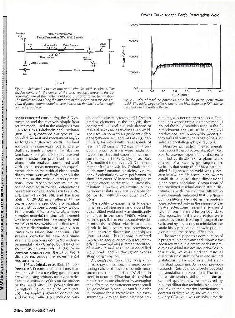
Fig. 4 — Plots of the (A) <002> and (B) <l 11> neutron diffraction intensities for the radial component of strain. The continuous line in (A) represents the best-fit approximation to the <002> intensity data.


was found in all of the samples sect ioned, despite the symmetry of the workpiece leads.

Real-Time Diagnostics

The efficiency of heat transfer from the arc to the part, i.e., process efficiency, was measured experimentally using a Seebeck calorimeter (Ref. 50). This efficiency represents the total energy absorbed by the part at the time of arc termination divided by the total arc energy. The average process efficiency, based on a total of three measurements, was 73% ±0.2% with the oxygen flow rates used. The efficiency in the absence of oxygen (<50 ppm) was 74%, based on two measurements.

Temperatures during welding were monitored using a combinat ion of chromel-alumel (K-type) and platinum-platinum/rhodium (R-type) thermocouples to span the temperature ranges of interest. Eighteen K-type thermocouples were spot welded to the back side of the specimen in a radial pattern along three of four perpendicular radii. Thermocouples were attached at increments varying from 0.3 mm (0.01 in.) near the center of the specimen, where the gradients were steepest, to 1.0 mm (0.04 in.) in the outer regions. The outermost thermocouples were 8.8 mm (0.35 in.) from the center of the specimen. On the top surface of the specimen, six R-type thermocouples were spot welded at distances ranging from 0.7 mm (0.03 in.) to 2.3 mm (0.09 in.) from the fusion boundary of the weld. In addition, two K-type thermocouples were welded at distances of 3.2 and 3.6 mm (0.13 and 0.14 in.) from the weld fusion boundary. The real-time temperature histories were recorded using two IBM-AT computers interfaced to a Keithley data acquisition unit. Data was taken at a rate of 50 measurements per s for the R-type thermocouples and at 20 measurements per s for the K-type

Table 2—Room Temperature Material Properties for the 304L

Static Young's modulus, E

Crystallographic elastic modulus <111>

<002> Poisson's ratio, j'buik

u <111> v <002>

0.2% offset yield

Proportional limit

198 GPa (longitudinal direction)

197 GPa (transverse direction)

307.7 GPa 100.8 GPa 0.28 (longitudinal) 0.28 (transverse) 0.111 0.373 188 MPa

(longitudinal) 183 MPa (transverse) 160 MPa

(longitudinal) 157 MPa (transverse)

thermocouples over a minimum time period of 60 s.

Neutron Diffraction Measurements

Description of the Technique

Neutron diffraction makes use of Bragg's law:

X= 2 dh k | sin©. Jhkl (D to relate the interplanar spacing, d ^ , of the plane (hkl) to the scattering angle, 2 0 ^ 1 , for the reflection and the wavelength, X. The normal to the diffraction plane lies along the scattering vector, which for elastic scattering bisects the incident and scattered beams. The presence of residual stresses, by changing d^ki, produces shifts in the diffraction peak positions, which can be interpreted as residual strains. An assessment of the residual stress in general requires measurements of all components of the strain tensor and a knowledge of the elastic constants. In the present case, it was assumed that the axial, hoop and normal components were the principal strains. The numerical analysis of strain was based on bulk, i.e., averaged polycrystalline elastic constants. In order to compare with the numerical calculations, we measured the residual elastic strains for both the (111) and (002) planes of the face-centered cubic stainless steel. The single crystal elastic constant for 304L stainless steel is stiffest, 307.7 GPa, for the <111> direction and softest, 100.8 GPa, for the <002> direction (Ref. 51). The Young's modulus (polycrystalline) elastic constant for the stainless steel bar-stock used in the experiment was 198 ±7 GPa in the axial direction and 197 ±8 GPa in the transverse direction (Ref. 52). By measuring the residual elastic strains in the <111 > and <002> directions, we were able to provide a bound on the polycrystall ine residual elastic strains calculated using Young's modulus.

The residual elastic strains in the GTA welded 304L stainless steel specimen were determined by measuring the d-spacing shifts in the lattice (Ref. 41) with respect to an unwelded specimen. Because neutrons readily penetrate 8 mm (0.31 in.) of steel nondestructively, neutron diffraction provided a through-thickness measure of the strain variation in the sample. This feature was critical to the analysis of the partial penetration weld, since there was a substantial variation in through-thickness strain in this geometry (Ref. 46).

Experimental Setup

The neutron diffraction strain measurements were made with a triple-axis crystal spectrometer at the NRU reactor in Chalk River. The spectrometer oper

ated as a high resolution diffractometer wi th incident and scattered neutron beams collimated to 0.1 and 0.2 deg, respectively, to obtain sharp diffraction peaks. The wavelength of the neutron beam, provided by the (113) planes of a Ge monochromator, was 2.6149 A. The incident beam was defined by a slit 1.5 mm (0.06 in.) wide and 2.0 mm (0.08 in.) high in an absorbing cadmium (Cd) mask. A similar slit 1.5 mm wide but 1 5 mm (0.6 in.) high defined the scattered beam. The diamond-shaped region of overlap of the incident and scattered beams that defined the gage volume, i.e., the volume in which the measurements are made, was 2.4 X 1.9 mm for the (111) reflections and 2.1 X 2.2 mm for the (002) reflection. The first dimension in each case is perpendicular to the scattering vector and the second dimension is parallel to it.

In order to derive strains from interplanar spacings, a "zero strain" reference sample was examined, which was 4 mm (0.16 in.) thick and had been cut from the same barstock as the welded sample. The strain is related to the d-spacing by the equation:

ehkl=(clhkl - dhkl,refVdhkl.ref (2)

The standard deviation of a single strain measurement was 1.0 X 10~4, whi le the experimental scatter from point to point was larger, on the order of 2.0 X 1 0 - 4 . The large experimental scatter, which was much worse than expected from counting statistics, was attributed to grain size effects and material inhomogeneities, such as the presence of 5 vol-% ferrite in the base metal (Ref. 46). In neutron diffraction measurements, the grains sampled in the diffraction measurement are those which fulfill the diffraction conditions wi th their plane normals oriented parallel to the bisector of the incident and scattered beams. In the presence of the large grains (1 00 to 1 50 microns) in the 304L barstock, the scatter in the intensity became significant, as shown by the scatter in the <002> and <111> intensities for the radial component of strain plotted in Fig. 4A and B. In this case, for a fixed gage volume of 2 mm 3 , the average number of grains with the correct orientation for diffraction in the gage volume was probably only 20 to 30 grains. As a result, only a small number of grains in the ensemble, each constrained by its neighboring grains, were sampled. Since the constraint provided by each set of different neighbors is different, scatter in the measured strains followed. The variation in intensity along a radial locus also indicates a variation in the grain orientation from the center to the edge of the specimen.

The room temperature properties


Residual Elastic Radial Strains (002) 10

'tn 8

8 -

5.6 mm

6.8 mm

-10 -8 - 6 - 4 - 2 0 2 4

Distance f r o m We ld Centerline (mm)

-80 -60 -40 -20 0 20

Distance f r o m We ld Centerline (mm) 40

0 20 40


Fig. 5 — Plots of the radial component of residual elastic strain. A — Near the as-solidified weld pool region as a function of depth through the sample, where the solid lines represent the best-fit curves generated from the raw neutron diffraction data; B and C — at the midplane of the specimen for the <002> and <l 11> diffraction conditions, respectively. The scans extend from the center of the specimen to the outer edge, or boss, of the specimen at a radial distance of 75.0 mm . The closed circles and open squares represent two different scans. The solid line represents the best-fit curve.

1 O

c co

c/5 o

••p 03

LU

"ro

• o 'c/3 <D

CC

o c I

10-

5 -

0 -

Residual Elastic Hoop Strains (002) Hoop

6.8 mm

5.6 mm A

4.0 mm / **., / V N

2.4 mm / / xT" " ^ S . 1.2 mm / , / / 'V . \ \ ..•

<£/ \ / %

—T T I i -15 -10 -5 0 5


10-

8 -

6 -

4 -

2 -

o-- 2 -

- 4 -

- 6 -

- 8 -B

(002) H

y*

•i i

• > JZf •

/* \*

/ D *D

1 !

• \

l 1

-80 -70 -60 -50 -40 -30 -20 -10 0 10 20 30 40

Distance f r om W e l d Centerline (mm)

~\ 1 1 r -80 -70 -60 -50 -40 -30 -20 -10 0 10 20 30 40 50

Distance f r o m W e l d Centerline (mm)

Fig. 6 — Plots of the hoop component of residual elastic strain. A — Near the as-solidified weld pool region as a function of depth through the sample, where the solid lines represent the best-fit curves generated from the raw neutron diffraction data; B and C — at the midplane of the specimen for the <002> and <lll> diffraction conditions, respectively. The scans extend from the center of the specimen to the outer edge, or boss, of the specimen at a radial distance of 75.0 mm. The closed circles and open squares represent two different scans. The solid line represents the best-fit curve.

WELDING RESEARCH SUPPLEMENT | 249-s

Normal Residual Elastic Strains (002)

Fig. 7— Plots of the normal component of residual elastic strain. A — Near the as-so

lidified weld pool region as a function of depth through the sample, where the solid

lines represent the best-fit curves generated from the raw neutron diffraction data; B and C — at the midplane of the specimen for the <002> and <111> diffraction conditions, respectively. The scans extend from the center

of the specimen to the outer edge, or boss, of the specimen at a radial distance of 75.0

mm. The closed circles and open squares represent two different scans. The solid line

represents the best-fit curve.

c 'co

O n S LJ "co 3

• g 'oj

OJ cc

-8

-10

-12

-14

-16

-58

-20

Normal

1.2 mm

2.4

4.0

5.6

6.8

V.

mm_

mm

mm

mm

• ' / /

— I 1 1 1 1 1 1 1 — 15 -12.5 -10 -7.5 -5 -2.6 0 2.5 5 7.5


o c

'co i

CO

T r -80 -70 -60 -50 -40 -30 -20 0 10 20 30 40 50


c 2 co

- | 1 1 r -80 -70 -60 -50 -40 -30 -20 -10 10 20 30 40 50


Table 3—Thermal Input Data

Heat flux distribution'3'

Arc efficiency factor,

Surface emissivity factor, i

Heat transfer coeff, h Latent heat of fusion,

Lf Latent heat of evap.,

Lv Kinetic evap.

efficiency, 7je'a> Thermal conductivity, (W/m-K), k

Solid ( T < 1673 K)

Liquid'3' (T > 1673 K)

(where f(T) increases linearly with temperature from 1 to 6 up to T = 3100 K)

Specific heat (J/kg-K), c Solid (T<1673 K) Liquid (T> 1723 K)

Gaussian, r2„ = 2.5 mm

90%

0.7 1.0 W / m 2 K

2.65 X 105 l /kg

7.35 X ICrVkg 20%

k = 8 .116+ 1.618 X 10~2T

k = f(T) X 35.2 (k @ 1673 K)

c = 465.4+ 0.1336T c = 788.

(a) Free parameters

used to interpret the neutron d i f f ract ion data for this mater ia l are shown in Table 2.

Residual elastic strain measurements in the par t ia l pene t ra t i on G T A w e l d were made at six depths relat ive to the top surface of the p late: 1.2, 2 .4 , 4 .0 , 4 .8 , 5.6 and 6.8 m m (0.05, 0 .09, 0 .16, 0 .19, 0.22 and 0.27 in.). A t each dep th , measurements w e r e taken in a l inear array start ing in the heat-affected zone ( H A Z ) region on one side of the w e l d , ex tend ing th rough the w e l d and con t i n u ing ou t to the restraining boss on the other side of the w e l d . Since each scan took a cons ide rab le a m o u n t o f b e a m t ime to o b t a i n the strains for a s ing le d i f f r a c t i o n c o n d i t i o n , o n l y a l i m i t e d number of points were sampled out to the boss region of the spec imen at the var ious depth levels. The most deta i led scan was done on the m idp lane of the spec imen, 4 .0 m m f rom the top surface. The rad ia l , h o o p and no rma l c o m p o nents of strain were de te rmined at each loca t ion .


Neutron Diffraction Results

The residual elastic strain distributions obtained for the radial, hoop and normal components of strain are presented in Figs. 5 through 7. In each figure, the top plot focuses on the strain variations occurring near the as-solidified weld pool region (up to 15.0 mm from the weld centerline) as a function of depth through the sample. The solid lines represent the best-fit curves generated from the raw neutron diffraction data. The subsequent plots in each figure, (B) and (C), show the residual strain distribution for the <002> and <111> diffraction conditions at the midplane of the specimen (4.0 mm from the top surface). The scans in each case extend from the center of the specimen to the outer edge, or boss, of the specimen at a radial distance of 75.0 mm (3.0 in.). Two different sets of measurements were made in each case, as indicated by the open squares and the closed circles. The closed circles give a survey at the mid-wal l position of the overall behavior, whereas the open squares concentrated on the behavior close to the weld. As in the top plot, the solid line represents the best-fit curve based on the raw data.

Figure 5A shows the distribution of radial strains near the weld pool zone for the <002> diffraction condi t ion. The residual elastic strains are tensile everywhere near the weld pool. At 5.6 and 6.8 mm below the top surface of the weld, the radial strains decrease sharply in the as-solidified weld pool region, which has a maximum radius of 4.5 mm along the top surface. At 6.8 mm from the top surface, the radial component of strain reaches a minimum of 4.0 X 1 0^* at the weld center ("0" location) increasing to greater than 10.0 X 10~4 around 8.0 mm from the weld centerline. At the very bottom of the the as-solidified weld pool region (4.0-mm depth) and within the weld (at 1.2 and 2.4 mm), there is very little variation in the radial strains wi th in ±10.0 mm of the weld centerline.

At distances greater than 10 mm from the weld centerline, the residual elastic radial strains at all depths decrease in magnitude. Figure 5B and C shows the distribution obtained from the weld centerline to the edge of the boss at a radius of 75 mm for the radial component of strain at a depth of 4.0 mm. The raw neutron diffraction measurements are shown in addition to the best-fit interpolation curve. The residual elastic radial strain distribution gradually decreases after 10.0 mm from the weld centerline, reaching a constant level at around 55.0 mm (2.2 in.) from the weld centerline — Fig. 5B and C. The final strains are tensile with a magnitude of 2.0 X 10~4 for both the <111> and <002> diffraction

SS304L TENSION TEST MODEL VS EXPERIMENT

(/> UJ

5

Symbols: Experimental Data

Lines: Model Predictions

0.2 0.3 0.4 0.5

TRUE STRAIN

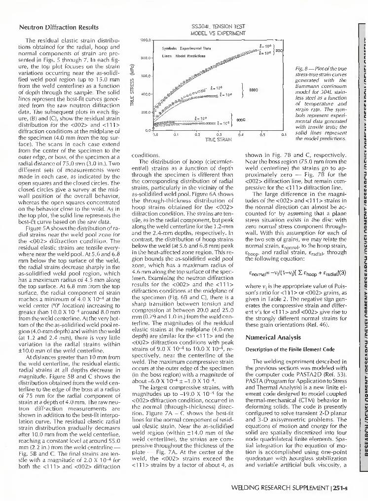
Fig. 8 — Plot of the true stress-true strain curves generated with the Bammann continuum model for 304L stainless steel as a function of temperature and strain rate. The symbols represent experimental data generated with tensile tests; the solid lines represent the model predictions-

conditions. The distribution of hoop (circumfer

ential) strains as a function of depth through the specimen is different than the corresponding distribution of radial strains, particularly in the vicinity of the as-solidified weld pool. Figure 6A shows the through-thickness distribution of hoop strains obtained for the <002> diffraction condition. The strains are tensile, as in the radial component, but peak along the weld centerline for the 1.2-mm and the 2.4-mm depths, respectively. In contrast, the distribution of hoop strains below the weld (at 5.6 and 6.8 mm) peak in the heat-affected zone region. This region bounds the as-solidified weld pool zone, which has a maximum radius of 4.6 mm along the top surface of the specimen. Examining the neutron diffraction results for the <002> and the <111 > diffraction conditions at the midplane of the specimen (Fig. 6B and C), there is a sharp transition between tension and compression at between 20.0 and 25.0 mm (0.79 and 1.0 in.) from the weld centerline. The magnitudes of the residual elastic strains at the midplane (4.0-mm depth) are similar for the <111 > and the <002> diffraction conditions with peak strains of 9.0 X 10"4 to 10.0 X 10"4, respectively, near the centerline of the weld. The maximum compressive strain occurs at the outer edge of the specimen (in the boss region) with a magnitude of about -6.0 X 1 ( H ± -1 .0 X 10"4.

The largest compressive strains, with magnitudes up to -19.0 X 10"4 for the <002> diffraction condition, occurred in the normal (through-thickness) direction. Figure 7A - C shows the best-fit lines for the normal component of residual elastic strain. Near the as-solidified weld region (within ±14.0 mm of the weld centerline), the strains are compressive throughout the thickness of the plate — Fig. 7A. At the center of the weld, the <002> strains exceed the <111 > strains by a factor of about 4, as

shown in Fig. 7B and C, respectively. Near the boss region (75.0 mm from the weld centerline) the strains go to approximately zero — Fig. 7B for the <002> diffraction line, but remain compressive for the <111 > diffraction line.

The large difference in the magnitudes of the <002> and <111 > strains in the normal direction can almost be accounted for by assuming that a plane stress situation exists in the disc with zero normal stress component through-wall. With this assumption for each of the two sets of grains, we may relate the normal strain, £norma | , to the hoop strain, ehoop' a n d radial strain, eracjia|, through the following equation:

enormal= —v/(" l—v i)[ £ £h o o p + £radia|](3)

where V; is the appropriate value of Pois-son's ratio for <111 > or <002> grains, as given in Table 2. The negative sign generates the compressive strain and different v's for <111 > and <002> give rise to the strongly different normal strains for these grain orientations (Ref. 46).

Numerical Analysis

Description of the Finite Element Code

The welding experiment described in the previous sections was modeled with the computer code PASTA2D (Ref. 53). PASTA (Program for Application to Stress and Thermal Analysis) is a new finite element code designed to model coupled thermal-mechanical (CTM) behavior in deforming solids. The code is presently configured to solve transient 2-D planar and 3-D axisymmetric problems. The equations of motion and energy for the solid are spatially discretized into four node quadrilateral finite elements. Spatial integration for the equation of motion is accomplished using one-point quadrature with hourglass stabilization and variable artificial bulk viscosity, a


RADIAL STRESS

TEMPERATURE TIME = 5 .32

TEMP 18E3 1 . 7 0 1 . 5 2 1 . 3 4 1 . 16 0 . 9 8 0 . 7 9 0 . 6 1 0 . 4 3 0 . 2 5

WM

wmm ,«H!lil

eSiSUl

wmm

RADIAL STRESS

B TEMPERATURE

TIME = 199 . 4 0

Fig. 9 — Graphical representation of the radial stress distribution and the temperature distribution in the partial penetration GTA weld. A — lust prior to arc termination; B — after cool down to ambient temperature. The bars at the right indicate the magnitude of stress in Pascals (Pa) and temperature in deg K.

Fig. 10 — Metallographic cross-section of the partial penetration GTA weld overlayed by a plot of the PASTA2D predictions of temperature. The "K" contour corresponds to the onset of melting at 1673 K. The "H" contour corresponds to the edge of the visible heat-affected zone at 1260 K. The temperature isotherms were computed using the optimized input parameters shown in Table 3. L= 181 OK, /= 1480K, F=986K, K=1670K, H=1260K, E=849K, l=1540K, G=1120K, D=712K.

technique similar to that utilized in other exclusively mechanical codes such as DYNA2D (Ref. 54) and PRONT02D (Ref. 55), Spatial integration for the energy equation is accomplished using a full four-point quadrature integration over the element. Energy transport within the solid is currently restricted to heat conduction only. The method for modeling the thermal part of the problem is similar to that used in heat conduction codes such as TACO (Ref. 56). Time integration of the equations of motion and energy are performed using the explicit time-centered-difference method (Ref. 57).

PASTA2D solves the coupled equations of motion and heat conduction. These equations are expressed as follows:

PV = V • cr + F (1)

pcpt = V • (kVT) + q (2)

in which p, o, F, c, k and q refer to the material density, stress state, body force per unit volume, heat capacity, isotropic thermal conductivity and heat of plastic work per unit volume, respectively. The superscript "dot" denotes the time derivative and the V the spatial derivative. The dependent variables v and T are the nodal velocities and temperatures calculated by PASTA2D. In the coupled thermal-mechanical mode, Equations 1 and 2 are solved simultaneously on a Lagrangian or moving mesh, which is mapped onto the deforming solid.

Heat generation due to plastic work is typically small compared to the boundary heat flux in the weld region for arc welding problems. Hence, the coupling between Equations 1 and 2 is not as strong as it would be in coupled thermal-mechanical metal forming problems. In large strain metal forming problems, the heat of plastic work causes a "two-way" coupling between the momentum and energy equations. Plastic deformation increases the heat of plastic work, q, causing localized temperature buildup which in turn affects mechanical properties. In welding problems, the thermal-mechanical coupling tends to be more "one-way," as described by Ar-gyris (Refs. 58, 59) since the temperature buildup is due primarily to an independent welding heat source or heat flux and not from the heat of plastic work.

In the present version of PASTA2D, Equations 1 and 2 are solved explicitly, making it possible to take full advantage of available vector processors. Explicit heat conduction codes permit solutions


(a) Thermal History on Top Surface near Fusion Boundary (b) Thermal History at Weld Centerline at Back Surface

1«00.0 1200.0

0.0 10.0 20.0 30.0 40.0 60.0 80.0 Time (seconds)

400.0

200.0

LEGEND PHSTR20

0.0 10.0 20.0 30.0 40.0 60.0 60.0 70.0 80.0 90.0 Time (seconds)

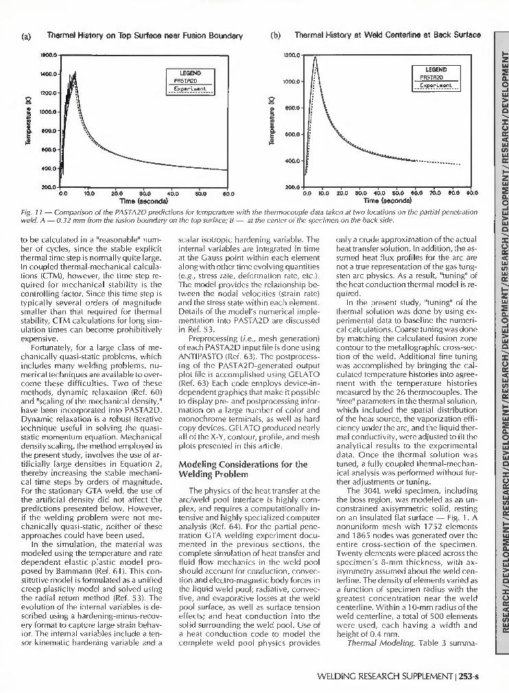
Fig. 11 — Comparison of the PASTA2D predictions for temperature with the thermocouple data taken at two locations on the partial penetration weld. A — 0.32 mm from the fusion boundary on the top surface; B — at the center of the specimen on the back side.

to be calculated in a "reasonable" number of cycles, since the stable explicit thermal time step is normally quite large. In coupled thermal-mechanical calculations (CTM), however, the time step required for mechanical stability is the controlling factor. Since this time step is typically several orders of magnitude smaller than that required for thermal stability, CTM calculations for long simulation times can become prohibitively expensive.

Fortunately, for a large class of mechanically quasi-static problems, which includes many welding problems, numerical techniques are available to overcome these difficulties. Two of these methods, dynamic relaxation (Ref. 60) and "scaling of the mechanical density," have been incorporated into PASTA2D. Dynamic relaxation is a robust iterative technique useful in solving the quasi-static momentum equation. Mechanical density scaling, the method employed in the present study, involves the use of artificially large densities in Equation 2, thereby increasing the stable mechanical time steps by orders of magnitude. For the stationary CTA weld, the use of the artificial density did not affect the predictions presented below. However, if the welding problem were not mechanically quasi-static, neither of these approaches could have been used.

In the simulation, the material was modeled using the temperature and rate dependent elastic-plastic model proposed by Bammann (Ref. 61). This constitutive model is formulated as a unified creep plasticity model and solved using the radial return method (Ref. 53). The evolution of the internal variables is described using a hardening-minus-recov-ery format to capture large strain behavior. The internal variables include a tensor kinematic hardening variable and a

scalar isotropic hardening variable. The internal variables are integrated in time at the Gauss point within each element along with other time evolving quantities (e.g., stress rate, deformation rate, etc.). The model provides the relationship between the nodal velocities (strain rate) and the stress state within each element. Details of the model's numerical implementation into PASTA2D are discussed in Ref. 53.

Preprocessing [i.e., mesh generation) of each PASTA2D input file is done using ANTIPASTO (Ref. 63). The postprocessing of the PASTA2D-generated output plot file is accomplished using GELATO (Ref. 63) Each code employs device-independent graphics that make it possible to display pre- and postprocessing information on a large number of color and monochrome terminals, as well as hard copy devices. GELATO produced nearly all of the X-Y, contour, profile, and mesh plots presented in this article.

Modeling Considerations for the Welding Problem

The physics of the heat transfer at the arc/weld pool interface is highly complex, and requires a computationally intensive and highly specialized computer analysis (Ref. 64). For the partial penetration GTA welding experiment documented in the previous sections, the complete simulation of heat transfer and fluid flow mechanics in the weld pool should account for conduction, convection and electro-magnetic body forces in the liquid weld pool; radiative, convective, and evaporative losses at the weld pool surface, as well as surface tension effects; and heat conduction into the solid surrounding the weld pool. Use of a heat conduction code to model the complete weld pool physics provides

only a crude approximation of the actual heat transfer solution. In addition, the assumed heat flux profiles for the arc are not a true representation of the gas tungsten arc physics. As a result, "tuning" of the heat conduction thermal model is required.

In the present study, "tuning" of the thermal solution was done by using experimental data to baseline the numerical calculations. Coarse tuning was done by matching the calculated fusion zone contour to the metallographic cross-section of the weld. Additional fine tuning was accomplished by bringing the calculated temperature histories into agreement with the temperature histories measured by the 26 thermocouples. The "free" parameters in the thermal solution, which included the spatial distribution of the heat source, the vaporization efficiency under the arc, and the liquid thermal conductivity, were adjusted to fit the analytical results to the experimental data. Once the thermal solution was tuned, a fully coupled thermal-mechanical analysis was performed without further adjustments or tuning.

The 304L weld specimen, including the boss region, was modeled as an unconstrained axisymmetric solid, resting on an insulated flat surface — Fig. 1. A nonuniform mesh with 1752 elements and 1 865 nodes was generated over the entire cross-section of the specimen. Twenty elements were placed across the specimen's 8-mm thickness, with ax-isymmetry assumed about the weld centerline. The density of elements varied as a function of specimen radius with the greatest concentration near the weld centerline. Within a 10-mm radius of the weld centerline, a total of 500 elements were used, each having a width and height of 0.4 mm.

Thermal Modeling. Table 3 summa-

WELDINC RESEARCH SUPPLEMENT 1253-s

Residual Elastic Radial Strains at 4.0 mm from Top Surface

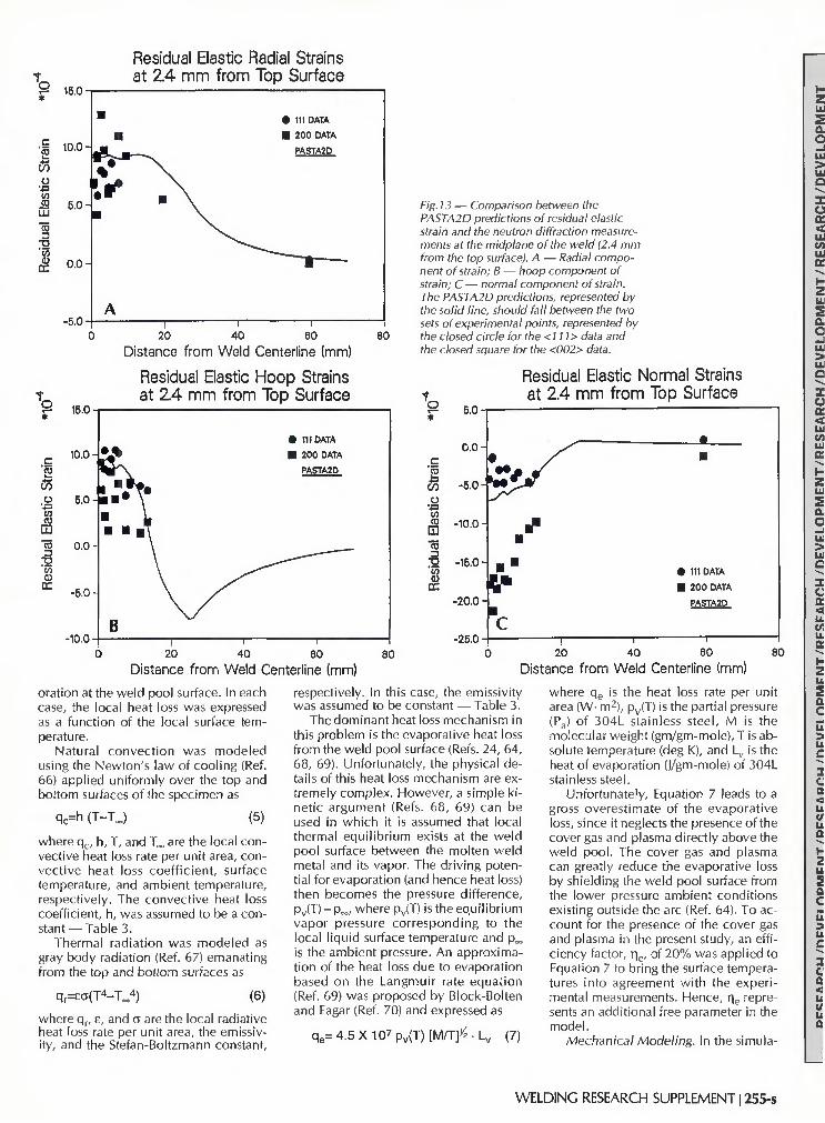
Fig. 12 — Comparison between the PASTA2D predictions of residual elastic

strain and the neutron diffraction measurements at the midplane of the specimen (4.0 mm from the top surface). A—Radial com

ponent of strain; B—hoop component of strain; C—normal component of strain. The

PASTA2D predictions, represented by the solid line, should fall between the two sets of experimental points, represented by the

closed circle for the <111> data and the closed square for the <002> data.

Residual Elastic Hoop Strains at 4.0 mm from Top Surface

c ra co ,o To c

to — ;-. C

ZZ

IO.U -

10.0-1

5 .0 -

0.0-

-5 .0 -

•

•

A i

•

• • v •

•

• •

• 111 DATA

• 002 DATA

PASTA

• •

1

• • •

*

C g

CO o

'*3 co CO

LU

"co 3

~0 co CD

cz

IU.U -

6.0-

0 .0 -

-5 .0 -

»ibu

-a

B

' • ¥* m

" : %

\y • i

• •

•

i

•

• 111 DATA

• 002 DATA

PASTA

•

• •

1 CO

LU

"9 •g

C8> o cz

5.0

0.0

-5.0

-10.0-

-15.0

20 40 60 Distance from Weld Centerline (mm)

Residual Elastic Normal Strains at 40 mm from Top Surface

80

-20.0 20 40 60

Distance from Weld Centerline (mm) 80

-

-

1

tf • ^ a

• •

• C

r

* a

• • 1

•

•

i

1

• •

• 111 DATA

• 002 DATA

PASTA

l

0 20 40 60 80 Distance from Weld Centerline (mm)

rizes the 304L thermal properties used in the model and the weld heat flux distribution parameters for the stationary GTA weld. The thermal properties in the melt were based on Argonne data (Ref. 65) for liquid 304L. The surface emissivity factor, e, and the heat transfer coefficient, h, were estimated from thermal data (Ref. 66) and held constant in the analysis, since they had little impact on the accuracy of the overall thermal solution. However, the liquid thermal conductivity was enhanced linearly with temperature for the reasons discussed below.

The gas tungsten arc heat source was modeled as a transient heat flux boundary condition applied to the top surface of the axisymmetric specimen at its center. The distribution of the heat flux was assumed to be Gaussian as described below:

Q(r,t)=na[3CUt)/jc r2c2]e-3[r/r 2<J 2 (4)

where r2a represents the radius within which 95% of the energy is transferred. This radius represented a free parameter in the heat source model.

The total power, Q„(t), in the Gaussian distribution was varied as a function of time according to the experimentally measured power curve — Fig. 2. A constant efficiency factor (r|a) of 90% was applied to the Gaussian distribution in order to account for radiative and other losses from the arc to the ambient environment, i.e., it was assumed that some portion of the energy (1 —r|a) leaving the electrode never reached the specimen surface. This efficiency factor represented another free parameter in the thermal model.

Heat transfer effects due to fluid flow in the weld pool were approximated by enhancing the temperature-dependent thermal conductivity, k(T), in the melt region, as done in previous work (Refs. 1 5, 24). In the current model, enhanced

thermal conduction was prescribed by linearly increasing k by a factor of 6 over the temperature range of 1673 to 3100 K. This linear enhancement provided the best fit of the melt isotherm to the fusion boundary determined in the metallographic cross-section. Hence, the effective thermal conductivity in the melt represented an additional free parameter in the present GTA weld model.

Phase change was approximated by defining a heat capacity curve with a discontinuity (Ref. 56). The latent heat of fusion due to melting and resolidification was taken into account through an appropriate step increase in the specific heat over the melting range of the 304L alloy (i.e., 1 673 to 1723 K).

Heat losses from the specimen surface were modeled as three distinct heat flux boundary conditions. The three boundary conditions accounted for: 1) natural convection, 2) thermal surface radiation, and 3) heat losses due to evap-


o 1 —

* ^ 15.0


-5.0 1 1 1 20 40 60



80

Fig. 13 — Comparison between the PASTA2D predictions of residual elastic strain and the neutron diffraction measurements at the midplane of the weld (2.4 mm from the top surface). A — Radial component of strain; B — hoop component of strain; C — normal component of strain. The PASTA2D predictions, represented by the solid line, should fall between the two sets of experimental points, represented by the closed circle for the <111> data and the closed square for the <002> data.

C co

CO CO

m "co D

g 'co

CD

cz

IO.U -

10.0-

6.0-

0.0-

-5.0-

10.0-

•%

• • • \ • L

" " " \

B i

• 111 DATA

• 200 DATA

PASTA2D

I "• "I

o

co y CO

m "to -g 'co

CD

cr

Residual Elastic Normal Strains at 2.4 mm from Top Surface

5.0-

0.0-

-6.0-

-10.0 -

-15.0 -

-20.0 -

-25.0

*****

a9

a • •

• C

t •

• 111 DATA

• 200 DATA

PASTA2D

20 40 60 Distance from Weld Centerline (mm)

80 20 40 60 Distance from Weld Centerline (mm)

80

oration at the weld pool surface. In each case, the local heat loss was expressed as a function of the local surface temperature.

Natural convection was modeled using the Newton's law of cooling (Ref. 66) applied uniformly over the top and bottom surfaces of the specimen as

qc=h (T-T. (5)

where qc , h, T, and T „ are the local convective heat loss rate per unit area, convective heat loss coefficient, surface temperature, and ambient temperature, respectively. The convective heat loss coefficient, h, was assumed to be a constant — Table 3.

Thermal radiation was modeled as gray body radiation (Ref. 67) emanating from the top and bottom surfaces as

q,=e0(T4-T„ (6)

where q r , e, and a are the local radiative heat loss rate per unit area, the emissivity, and the Stefan-Boltzmann constant,

respectively. In this case, the emissivity was assumed to be constant — Table 3.

The dominant heat loss mechanism in this problem is the evaporative heat loss from the weld pool surface (Refs. 24, 64, 68, 69). Unfortunately, the physical details of this heat loss mechanism are extremely complex. However, a simple kinetic argument (Refs. 68, 69) can be used in which it is assumed that local thermal equilibrium exists at the weld pool surface between the molten weld metal and its vapor. The driving potential for evaporation (and hence heat loss) then becomes the pressure difference, pv(T) - p^, where pv(T) is the equilibrium vapor pressure corresponding to the local liquid surface temperature and p^ is the ambient pressure. An approximation of the heat loss due to evaporation based on the Langmuir rate equation (Ref. 69) was proposed by Block-Bolten and Eagar (Ref. 70) and expressed as

qe= 4 .5X107 pv(T) [M/T]^ • Lv (7)

where qe is the heat loss rate per unit area (W- m2), pv(T) is the partial pressure (Pa) of 304L stainless steel, M is the molecular weight (gm/gm-mole), T is absolute temperature (deg K), and Lv is the heat of evaporation (J/gm-mole) of 304L stainless steel.

Unfortunately, Equation 7 leads to a gross overestimate of the evaporative loss, since it neglects the presence of the cover gas and plasma directly above the weld pool. The cover gas and plasma can greatly reduce the evaporative loss by shielding the weld pool surface from the lower pressure ambient conditions existing outside the arc (Ref. 64). To account for the presence of the cover gas and plasma in the present study, an efficiency factor, r|e, of 20% was applied to Equation 7 to bring the surface temperatures into agreement with the experimental measurements. Hence, r|e represents an additional free parameter in the model.

Mechanical Modeling. In the simula-


o

g 'co I—

CO y '& CO

JO LU

"a -g 'co CD LT

Fig. 14 — Comparison between the PASTA2D predictions of residual elastic

strain and the neutron diffraction measurements at 1.2 mm from the top surface. A —

Radial component of strain; B — hoop component of strain; C — normal component of

strain. The PASTA2D predictions, represented by the solid line, should fall between

the two sets of experimental points, represented by the closed circle for the <111> data and the closed square for the <002>

data.


10.0-

• I

6.0-

0 .0 -

-5 .0 -

B ^ i

• 111 DATA

• 200 DATA

PASTA2D

g CO

CO

oo co

Qj

"co a • g

CO o cz


*

c CO

co n Vt CO

UJ

"to -1

X3 CO o rr

10.0-

5.0-

0 . 0 -

•

F/-N

* * \

' * • \

• • A

i

• 111 DATA

• 002 DATA

PASTA

l i

20 40 60

Distance from Weld Centerline (mm) 80

Residual Elastic Normal Strains at 1.2 mm from Top Surface

D.U "

0 .0 -

- 5 . 0 -

10.0-

•1B0-

s'

m /

m

a

* i

• 111 DATA

• 200 DATA

PASTA2D

I l 20 40 60

Distance from Weld Centerline (mm) ec 0 20 40 60 80


Table 4—Calculated and Measured Peak Temperatures As a Function of Distance from the Weld Centerline

Surface

Top Top Back Back

Distance from

Centerline

5.4 mm 7.66 mm 0.36 mm 5.76 mm

Calculated Temp

eratures

1328 K 909.7 K

1181 K 863.4 K

Measured Temp

eratures

1313 K 874 K

1107 K 824 K

Note-Weld pool radius was 4.6 mm

tion, the 304L specimen was modeled as an unrestrained body and allowed to slide freely along the bottom surface of the restraining boss — Fig. 1. The thermal-mechanical behavior of the 304L specimen was simulated using the rate and temperature dependent elastic-plastic continuum model discussed above. The material constants required for the

constitutive model were obtained from torsion and uniaxial tension test data generated at a series of different strain rates and temperatures up to melt for 304L stainless steel (Refs. 61 , 72). Near melt, the Young's modulus was reduced to less than 1 MPa, to approximate the zero strength of the melt. The quality of the fit is demonstrated in Fig. 8, which shows temperature and strain-rate dependent true stress-true strain curves over a range of temperatures.

In order to compare the residual elastic strains measured with neutron diffraction to the residual elastic strains computed in PASTA2D, the calculated strains accumulated during heating of the molten weld pool region had to be zeroed at the time of resolidification. In addition, the cool-down period in the model had to be sufficient for the weld energy to diffuse throughout the specimen via heat conduction, thus eliminating the thermal elastic strain component.

The time required for the welded 304L specimen to come to a nearly isothermal ambient temperature everywhere in the mesh was approximately 200 s (5 s of arc-on t ime and 195 s of cool-down time). Shorter simulation times could have been achieved by a simulated rapid quench from some higher temperature, as was done in previous studies (Ref. 35). However, this approach was avoided to ensure that the history dependent internal variables in the constitutive relationship would evolve properly.

Comparison of Numerical Predictions with Experimental Measurements

Figure 9A and B show graphical representations of the predicted radial stress and temperature distributions in the part at the time of arc termination and after cool down to room temperature, respectively. The axial displacements were

256-s I SEPTEMBER 1991

magnified by 100% (i.e., doubled) in these figures in order to emphasize the weld region. The rounded appearance of the top surface of the molten weld pool zone resulted from the assumption that the molten material could support an extremely small deviatoric stress. This assumption was required to ensure computational stability. Although only the radial component of stress is represented in Fig. 9Aand B, all components of stress were calculated.

Temperature Comparisons

In the thermal model, adjustments of the thermal parameters, i.e., the isotropic l iquid thermal conductivi ty -k(T), the 2<j radius - r2 a , and the heat loss parameters (r|e, r|a, h, and e), resulted in an as-solidified weld pool region (fusion zone boundary) approximately equal to that which was observed experimentally through metallographic cross-sectioning of the weld. Variations in h and e had little effect on the weld pool shape and size, while variations in k(T), r2o, and r\e (Table 3), had a considerable influence on weld pool geometry. Wherever possible, physically "reasonable" values for the parameters were selected (Refs. 65, 66, 73). In the molten region, it was difficult to select reasonable values for r\e and k(T), since the evaporative loss model and the weld pool heat transfer model were not representative of the true physics.

The parametric studies required to "tune" the thermal solution were done by running the thermal portion of the calculation without activating the mechanical portion of PASTA2D. This resulted in a substantial savings in computer time. Figure 10 shows a cross-section of the actual GTA weld overlayed with the best fit temperature isotherms predicted at the time of arc termination. The spatial position of the calculated 1673 K isotherm, which is the lower bound of melt in 304L stainless steel, was fit to the fusion zone boundary on the metallographic cross-section. The edge of the dark etching heat-affected zone region is associated with the calculated 1260 K contour line. Although matching the fusion zone boundary ensures that the energy in the analysis has been deposited in such a way as to produce at least one isotherm in the right place at the right time, it does not ensure correct partitioning of the energy within the weld pool, nor does it ensure correct growth and decay rates for the fusion boundary, particularly for convex weld pools.

In order to further evaluate the effectiveness of the tuning in the thermal solution, the calculations were compared with a number of measured thermocouple histories outside of the weld zone.

Table 4 shows the peak temperatures calculated at various nodes and the corresponding peak temperatures as a function of location recorded experimentally.

The agreement between the calculated and measured temperature histories at all locations was typical of the agreement shown in Fig. 11A and B. The experimental noise associated with the thermocouple nearest the fusion boundary is caused by the electrical noise from the arc. As indicated by these figures, the correlation is excellent, even near the fusion boundary. In most cases, the small differences in peak temperature were on the order of the error (+ 0.3 mm) associated with precisely matching node locations (where temperatures were calculated) with thermocouple locations (where temperatures were measured). Differences in the calculated temperature histories between the coupled thermal-mechanical calculation and the thermal-only calculation were small (less than 30 K), indicating that the thermal-mechanical analysis could have been performed uncoupled — i.e., results from the fixed grid heat conduction solution could have been used as input for the mechanical analysis.

After "tuning" the thermal parameters, the calculated process efficiency for this problem was 6 1 % . This efficiency did not agree with the experimentally determined efficiency of 73%, obtained using the Seebeck calorimeter (Ref. 50). Considering this disagreement, the good correlation in temperature histories is surprising. Underprediction of the process efficiency may be related to how the model partitioned the energy i n the weld pool. As mentioned previously, the analytical model accounts for heat transfer effects in the molten region using an enhanced thermal conductivity. This is not a true representation of the fluid flow in the weld pool. Other factors, such as the evaporation model, may have also contributed to underprediction of the process efficiency.

The sole purpose of adjusting the free parameters in the thermal solution was to provide a means of depositing the CTA weld energy in the workpiece in approximately the right place at the right time. Once this was accomplished, the ability of the numerical model to predict the residual elastic strain distribution in the as-welded specimen could be assessed. Calculations of the thermal strains generated during and after welding were made without further parametric adjustments.

Residual Elastic Strain Comparison

Verification of the code predictions was based on comparison of the residual

elastic strains, rather than on comparison of the residual stresses, although the code calculates both. Conversion of the experimentally measured elastic strains into their corresponding stresses was attempted using both the Reuss method and the Voigt method (Refs. 74, 75). However, the resultant stresses obtained from these two methods were not equal. To avoid ambiguity in the comparison, calculated and measured residual elastic strains rather than stresses were compared to assess the accuracy of the finite element predictions.

The polycrystalline residual elastic strains calculated in PASTA2D were compared with the residual elastic strain data determined by neutron diffraction from both the <111> and the <002> diffraction conditions. As discussed previously, the two different diffraction conditions were selected to provide an upper and lower bound on the range of residual elastic strains measured crystal-I ©graphically.

The agreement between the computer predictions and the experimental measurements can be readily evaluated by comparing the residual elastic strains in the partial penetration weld at various depths in the specimen. Although a number of comparisons were made through the thickness of the specimen, only three depths (1.2 , 2.4 and 4.0 mm from the top surface) are discussed here. Planes corresponding to each of these depths intersect a portion of the as-solidified weld pool.

Figure 1 2A through C shows the residual elastic strain data predicted and measured at the midplane of the specimen (4.0 mm from the top surface). This plane intersects the very bottom of the partial penetration weld. The prediction for the radial component of strain (Fig. 12A) falls wel l w i th in the strain levels bounded by the crystallographic measurements everywhere in the specimen. For the hoop and normal components of strain (Fig. 12B and C), the agreement is equally good except at a distance of 0.025 m (1 in.) from the weld centerline. In this location, the predicted elastic normal strain overshoots the experimental data slightly — Fig. 12C. Due to equilibrium of stress inherent in the calculations, the predicted elastic hoop strains correspondingly fall slightly below the experimental measurements, as indicated by Fig. 12B.

The comparisons between the measured and predicted residual elastic strains near the midplane of the weld (2.4 mm from the top surface) are similar to the comparisons made at the midplane of the specimen (4.0 mm from the top surface). As indicated in Fig. 1 3A through C, the computer predictions again fall within the region bounded by


the experimental data. No diffraction measurements were made at 25 mm from the weld centerline, which would allow us to determine how well the calculations tracked the data in this region. However, there is good agreement between the calculations and the measurements at 0.06 m (2.4 in.) from the weld centerline — Fig. 1 3A and C.

At the 1.2-mm depth, the neutron diffraction data was collected only out to a radius of 1 5 mm (0.6 in.) from the weld centerline. Figure 14A - C shows comparisons of the predicted strain distributions with experimental measurements at the 1.2-mm depth. Little can be said about the far-field strain comparisons at this depth. However, in the range where data was collected, the agreements are comparable to that obtained at the previously discussed depths.

Since the PASTA2D calculations are based on isotropic polycrystalline properties, the strains measured for <111> and <002> orientations should bound the finite element calculations. Within the as-solidified weld pool, however, a large degree of anisotropy exists due to the preferred growth of <002> grains (Refs. 45, 46). As a result of this anisotropy, the correlation between the computer predictions and the experimental measurements in the as-solidified weld pool is less quantitative than in the heat-affected zone and beyond. This is readily evident in the plots of residual elastic normal strains (Fig. 14A and C), where the measured <002> strain values fall consistently below the predicted strain values. In the near field region of the as-solidified weld pool (<10.0 mm/0.4 in. from the weld centerline), a "waviness" is apparent in all three predicted components of elastic strain. At this time, we do not have a good feel for how real this behavior may be. Due to the scatter in the neutron diffraction measurements, it is difficult to determine whether the same behavior occurs experimentally.

Conclusions

In the present simulation, a heat conduction model was used to predict the energy deposition in a stationary partial penetration GTA weld. Since the conduction model ignores much of the physics of the weld pool heat transfer, "tuning" of the thermal heat conduction solution during the arc-on time was required to bring the predicted fusion zone and temperature distributions into agreement with experiment. The free or primary parameters used in tuning the thermal calculation included the heat loss from the arc to the environment, the heat loss due to evaporation, the 2o radius of the assumed Gaussian heat source, and

the thermal conductivity in the molten weld pool. Of these parameters, the last three had the most effect on weld pool shape and size, as well as on predicted process efficiency.

The purpose of adjusting the thermal solution was to ensure that the energy deposited in the finite element mesh was approximately the same as that deposited in the experimental workpiece. Having done this, calculations were performed using a temperature and rate dependent visco-elasto-plastic constitutive model to determine the residual elastic strains in the as-welded specimen of 304L stainless steel. In order to verify the computer predictions, neutron diffraction measurements were taken at a variety of locations within the specimen. These measurements provided through-thickness as well as radial variations in strain, at a number of locations. Comparisons of the neutron diffraction data with the computer predictions indicated that the agreement was excellent both in the weld pool region and near the edge of the specimen, at least to the scale of resolution obtainable experimentally. The assumption of isotropic mechanical properties for the as-solidified weld pool had less influence on the residual strain prediction than anticipated.

Based on the above results, it is evident that future work should be directed towards coupling a fluid flow model into the thermal-mechanical analysis and improving our ability to account for the arc/weld pool physics. Improvement of the f luid f low model would provide more realistic temperatures for evaluation of the solidification microstructure and for penetration predict ion. This work should first be performed on simple configurations such as the axisymmetric stationary weld. Extension of this work to a traveling GTA weld wil l require a three-dimensional, thermal-fluid-mechanical analysis. Experimentally, effort needs to be directed toward refining the material property data available for input into the computer models and toward improving our abil i ty to measure temperature and electric field distributions in the arc itself. Additional theoretical work is also required to improve the kinetic vaporization and surface tension models for the molten weld pool.

Acknowledgments

The authors would like to thank J. Krafcik for his design of the data acquisition system, R. Blum of SNLL for his help in the experimentation, D. J. Bam-mann for his contributions to the material modeling, P. Fuerschbach of SNLA for his measurements of process efficiency, and the Chalk River Nuclear

Group for their help in determining material properties and texture information needed for reduction of the neutron diffraction data. We would also like to thank J. Brooks, R. Rohde, and C. W. Robinson for their continued support of this work. This work is supported by the U. S. Department of Energy, DOE, under Contract No. DEAC04-76DP00789.

References

1. Tall, L. 1964. Residual stresses in welded plates — a theoretical study. Welding lournal43CD-A0-S to 23-s.

2. Fujita, Y., Nomoto, T., and Hasegawa, H. 1980. Method of thermal elasto-plastic analysis (4th report). Naval Arch, and Ocean Eng. 18:164-174.

3. Muraki, T., Bryan, J.)., and Masubuchi, K. 1975. Analysis of thermal stresses and metal movement during welding—Parts I and II. Journal of Eng. Materials and Tech. ASME, pp. 81-91.

4. Rybicki, E. F., Schmueser, D. W., Stone-sifer, R. B. , Groom, J. J., and Mishler, H. W. 1978. A finite element model for residual stresses and deflections in girth-butt welded pipes, lournal of Press. Vessel Tech. ASME 100:256-262.

5. Pavelic, V., Tanbakuchi, R., Uyehara, O. A., and Meyers, P. S. 1969. Experimental and computer temperature histories in GTA welding in thin plates. Welding lournal 48(7):295-s to 305-s.

6. Ueda, Y., and Yamkawa, T. 1972. Thermal nonlinear behavior of structures. Advances in Computer Methods in Structural Mechanics and Design, ed. J. T. Oden, R. Clough, and Y. Yamamoto, UAH Press, pp. 375-392.

7. Hibbitt, H. D., and Marcal, P. V. 1973. A numerical thermo-mechanical model for the welding and subsequent loading of a fabricated structure. Computers and Structures 3:1145-1174.

8. Nickell, R. E., and Hibbitt, H. D. 1975. Thermal and mechanical analysis of welded structures. Nuclear Eng. and Design 32:110-120.

9. Hibbitt, H. D. 1976. Thermomechanical analysis of welded joints and structures. Advances in Joining Technology, ed. I. I. Burke, A. E. Gorum, and A. Tarpinian, Brook Hill Publishing Co., Chestnut Hill, Mass., pp. 357-377.

10. Karlsson, L. 1976. Stress fields induced by moving heat sources in butt welding of plates. Ph.D. Thesis, Chalmers Univ. of Technology, Sweden.

11. Friedman, E. 1975. Thermomechanical analysis of the welding process using the finite element method, lournal Press. Vessel Tech. ASME, Series J, 97(3):206-21 3.

12. Glickstein, S. S., and Friedman, E. 1979. Temperature and distortion transients in gas tungsten arc weldments. DOE Res. and Develop. Report WAPD-TM-1428.

13. Glickstein, S. S. 1982. Basic studies of the arc welding process. Trends in Welding Research in the U.S., ed. S. A. David, ASM International, Materials Park, Ohio, pp. 3-51.

14. Ueda, Y., Takahasi, I., Fukuda, K., Sakamoto, K„ and Nakacho, K. 1976. Multipass welding stresses in very thick plates and


their reduction from stress relief annealing. Trans, of Japan Weld. Res. Inst. 5(2):79-89.

15. Duncan, D. B. 1980. Thermo-me-chanical modeling of the gas tungsten arc welding process. M. S. Thesis, University of California, Davis, Calif.

16. Masubuchi , K. 1980. Analysis of welded structures. Int'l Series on Mat. Sci. and Tech. Vol. 33, Pergamon Press.

17. Papazoglou, V. ). 1981. Analytical techniques for determining temperatures, thermal strains, and residual stresses during welding. Ph.D. Thesis, MIT., Cambridge, Mass.

1 8. Masubuchi, K., and Agapakis, j . 1 982. Analysis and control of residual stresses, distortion and their consequences in welded structures. Trends in Welding Research in the U.S., ed. S. A. David, ASM International, Materials Park, Ohio, pp. 153-172.

19. Ueda, Y„ and Nakacho, K. 1982. Simplifying methods for analysis of transient and residual stresses and deformations due to multipass welding. Trans. Japan Weld. Res. Inst. 11:95-103.

20. Eagar, T. E., and Tsai, N. -S. 1983. Temperature fields produced by traveling distr ibuted heat sources. Welding Journal 62(12):346-sto355-s.

2 1 . Goldak, J. A., Patel, B., Bibby, M. J., and Moore, J. E. 1985. Computational weld mechanics. AGARD (NATO) Advanced Joining of Aerospace Metallic Materials,CP-398, (N87-1 7052/8), pp. 1.1-1.32.

22. Patel, B. 1985. Thermo-elasto-plastic finite element analysis of deformation and residual stresses due to welds. Ph.D. Thesis, Carleton University, Ottawa, Canada.

23. Chakravarti, A. P., Malik, L. M., and Goldak, J. A. 1986. Prediction of distortion and residual stress in panel welds. Symposium on Computer Modelling of Fabrication Processes and Constitutive Behavior of Metals, ed. j . Too, Ottawa, Canada.

24. Mahin, K. W., Shapiro, A. B., and Hall-quist, J. 1986. Assessment of boundary, condit ion limitations on the development of a general computer model for fusion welding. Advances in Welding Science and Technology, ed. S.A. David, ASM International, Materials Park, Ohio, pp. 215-224.

25. Newman, S. Z. 1986. FEM model of 3D transient temperature and stress fields in welded plates. Ph.D. Thesis, Carnegie-Mellon University, Pittsburgh, Pa.

26. Andersson, B. A. B. 1978. Thermal stresses in a submerged arc welded joint considering phase transformations. Journal Eng. and Tech., ASME, 100:356-362.

27. Andersson, B., and Karlsson, L. 1981. Thermal stresses in large butt-welded plates. J. Thermal Stresses (41:491-500.

28. Lindgren, L. 1985. Deformation and stresses in butt-welding of plates. Ph.D. Thesis, Lulea University of Technology, Sweden.

29. Jonsson, M., Karlsson, L., and Lindgren, L-E. 1 984. Thermal stresses, plate motions and hot cracking in butt-welding. Proc. Int'l. Conf. on Mech. Behav. of Matls. (Stockholm), ed. J. Carlsson and H-G. Ohlson, Pergamon Press, Oxford, England, pp. 273-279.

30. Jonsson, M., Karlsson, L. and Lindgren, L. -E. 1985. Deformations and stresses in butt-welding of large plate. Num. Methods in Heat Transfer, ed. by R. W. Lewis, J. Wiley & Sons, Ltd., Ch. 2., pp. 35-58.

3 1 . Karlsson, L. 1986. Thermal Stresses I, 2nd series, Vol. 1. Ch. 5. ed. R. R. B. Hetnarsk, Elsevier Science Publishers.

32. Troive, L.. Karlsson. L., and Nasstrom, M. 1989. Finite element simulations of the bending of a flat plate to u-shaped beam cross-section and the welding to rectangular hollow cross-section. Proc. of the 2nd Int'l Conf. on Trends in Welding Research, ed. S. A. David and ). Vitek. ASM International, Materials Park, Metals Park, Ohio.

33. lonsson. M.. losefson, B. F. 1988. Experimentally determined transient and residual stresses in a butt-welded pipe. Journal Strain Analysis for Eng. Design 23(1 ) :25-31.

34. Goldak, |. A.. Oddy, A., McDi l l , M., Chakravarti, A., Bibby, iM. J., and House, R. 1986. Progress in computing residual stress and strain in welds. Advances in Welding Science and Technology, ed. S. A. David, ASM International, Materials Park, Oh io , pp. 523-527.

35. Goldak, J. A., Chakravarti, A., Bibby, M. ). 1984. A new finite element model for welding heat sources. Trans AIME, 15B(6):299-305.

36. Goldak, ). 1989. Model ing thermal stresses and distortions in welds. Proc. of the 2nd Int'l Conf. on Trends in Welding Research, ed. S. A. David, ASM International, Materials Park, Ohio.

37. Oddy, A., McD i l l , M., Goldak, ). 1989. A general transformation plasticity relation for 3-D finite element analysis of welds, submitted to Euro. I Mechanics.

38. Mahin, K. W., MacEwen, S., Winters, W. S., Mason, W.E., Kanouff, M., and Fuchs, E. A. 1988. Evaluation of residual stress distributions in a traveling GTA weld using finite element and experimental technique. Modeling and Control of Casting and Welding Processes IV, ed. A. Giamei, TMS-AIME, pp. 339-350.

39. Mahin, K. W., MacEwen, S., Winters, W. S., Mason, W. E., Fuchs, E.A. I 989. Finite element modeling and experimental verification of residual strain distributions in GTA welds. Proc. of 2nd Int'l Conf. on Trends in Welding Research, ed. S. A. David and J. Vitek, ASM International, Materials Park, Ohio, pp. 8 3 - 9 1 .

40. Corrigan, D. A. 1966. Thermomechanical Effects in Fusion Welding of High Strength Steels" Ph.D. Thesis, MIT, Cambridge, Mass.

4 1 . Pintschovius, L., and lung, V. 1983. Residual stress measurement by means of neutron di f fract ion. Mat. Sci. and Eng. 61:455-464.

42. MacEwen, S. R., Holden, T. M., Powell, B. M., Lazor, R. B. 1987. Residual strains in girth-welded line pipes. Welding Metallurgy of Structural Steels, ed. J. Kou, TMS-AIME, pp. 455-464.

43. Holden, T. M., Powell, B. M., and MacEwen, S. R. 1987. Axial strains at a girth weld in a 914 mm linepipe. Nondestructive Characterization of Materials II, ed. ]. F. Bussiere, J. -P. Monchalin, C. O. Ruud and R. E. Green, Jr., Plenum Publishing Co., pp. 625-631.

44. Holden, T. M., Root, J. H., Fidleris, V., Holt, R. A., and Roy, G. 1 988. Application of neutron diffraction to engineering problems. Mat. Sci. Forum, 27, 28:359-370.

45. Holden, T. M., Hosbons, R. R., Root,

I. H., MacEwen, S. R. 1989. Residual stresses in a single pass weld in a 304L stainless steel plate. ANDI-31, Chalk River Nuclear Labs, Canada.

46. Holden, T. M „ Hosbons, R. R., MacEwen, S. R., and Parsons, D. V. 1989. Neutron diffraction measurements of the distribution of residual strains in and near stationary gas tungsten arc welds in 304 stainless steel. ANDI-32, Chalk River Nuclear Labs, Canada.

47. Heiple, C. R., and Roper, J. R. 1982. Mechanism for minor element effect on GTA fusion zone geometry. Welding Journal 61(4):97-sto 102-s.

48. Walsh, D. W. 1986. Minor Element Effects on Gas Tungsten Arc Welds. Ph.D. Thesis, Rensselaer Polytechnic Inst., New York, pp.298.

49. Sahoo, P., Debroy, T., and McNallan, M.). 1 988. Surface tension of binary metal — surface active solute systems under conditions relevant to welding metallurgy. Met. Trans. B 19B(6):483-491.

50. Knorovsky, G. A., and Fuerschbach, P. W. 1986. Calorimetry of pulsed versus continuous gas tungsten arc welds. Advances in Welding and Technology, ed. S. A. David, ASM International, Materials Park, Ohio, pp. 393-399.

51 . Kikuchi, M. 1971. Elastic anisotropy and its temperature dependence of single crystals and polycrystal of 18-12 type stainless steel. Trans, of Jpn. Inst. of Metals, 12:417-421.

52. Mecke, J. 1989. Private communication, Chalk River Nuclear Laboratories, Chalk River, Ontario, Canada.

53. Winters, W. S., and Mason, W. E. 1989. PASTA2D-applications. SAND89-8217, Sandia National Laboratories, Livermore, Calif.

54. Hallquist, J. O. 1980. User's manual for DYNA2D — an explicit two-dimensional hydrodynamic finite element code with interactive rezoning. UCID-18756, University of Cali fornia, Lawrence Livermore National Laboratory, Livermore, Calif.

55. Taylor, L. M., and Flanagan, D. 1 987. PRONT02D, a two-dimensional transient solid dynamics program. SAND86-0594, Sandia National Laboratories, Albuquerque, N. Mex.

56. Mason, W. E. 1983. T A C 0 3 D — a three-dimensional finite element heat transfer code. SAND 83-8212, Sandia National Laboratories, Livermore, Calif.

57. Belytachko, T. 1983. An overview of semidiscretization and time integration procedures. Computational Methods for Transient Analysis, Vol . 1, North-Holland, New York, N.Y.

58. Argyris, J. H., Vaz, L. E„ and Wil l iam, K. J. 1981. Integrated finite-element analysis of coupled thermoviscoplastic problems. Journal Thermal Stresses 4:121-1 53.

59. Argyris, J. H., Szimmat, L. E., and Wil l iam, K. J. 1982. Computations aspects of welding stress analysis. Comp. Methods Appl. Mech. Eng. 33:635—666.

60. Underwood, P. 1983. Dynamic relaxation. Computational Methods for Transient Analysis, Vol. 1, North-Holland, New York, N.Y.

61 . Bammann, D. |. 1989. Parameter determination for a strain rate and temperature

WELDING RESEARCH SUPPLEMENT | 259-s

dependent plasticity model. SAND89-8812, Sandia National Laboratories, Livermore, Calif.

62. Nielan, P. E., Perano, K. J., and Mason, W. E. 1990. ANTIPASTO: an interactive mesh generator and preprocessor for two-dimensional analysis programs. SAND90-8203, Sandia National Laboratories, Livermore, Calif.

63. Mason, W. E. 1988. GELATO—an interactive finite element postprocessor. Internal report, Sandia National Laboratories, Livermore, Calif.

64. Lancaster, J. F. 1984. Physics of Welding, IIW, Pergamon Press, Oxford, England.

65. Leibowitz, L. 1976. Properties for LMFBR safety analysis. ANL-CEN-RSD-76-1, p. 116.

66. Touloukian, Y. S., and Ho, C. Y. 1970. Thermophysical Properties of Selected Aerospace Materials—Thermal Radiative Properties, Purdue University, Lafayette, Ind.

67. Kreith, F. 1973. Principles of Heat Transfer, Harper & Row, Publishers, Inc., New York, N.Y.

68. Shapiro, A. B. and Mahin, K. W. 1987. Thermomechanical Modeling of Gas Tungsten Arc Weld ing, lournal of Eng. Comp. and Applications, 1 (4):28-34.

69. Dushman, S. 1962. Scientific Foundations of Vacuum Technique, John Wiley and Sons, 2nd ed., New York, N.Y.

70. Block-Bolten, A., and Eagar, T. W. 1984. Metal vaporization from weld pools. Met. Trans B, 15B:461-469.

7 1 . Bertram, L. A., and Mahin, K. W. 1 989. Fluid dynamics in material processing:

a weld ing simulat ion. Fluids Engineering Seminar Korea-US Progress, ed. J. H. Kim, J. M. Hyun and C-O. Lee, Hemisphere Publishing, pp. 545-558.

72. Mahin, K. W. Unpublished data. 73. Mcl lwain, M. E., Smartt, H. B., Stew

art, J. A., and Einerson, C. J. 1985. Characterization of the heat source distribution of a typical GTAW welding arc. Proc. of SPIE— The International Society for Optical Engineering, 520:102-105.

74. Reuss, A. 1929. Berechnung der Fliesgrenze von Mischkristallen auf Grund der Plastizitatsbedingung fur Einkristalle. Z. Agnew Math. Mech. 9:49-58.

75.Voigt, W . 1928. LehrbuchderCristal-physik. B. G. Tubnerverlag, Leipzig.

WRC Bulletin 361 February 1991

This Bulletin contains two reports that compare the French RCC-M Pressure Vessel Code and the U.S ASME Section III Code on Design of Nuclear Components and Piping Design Rules.

(1) Improvements on Fatigue Analysis Methods for the Design of Nuclear Components Subjected to the French RCC-M Code

By J. M. Grandemange, J. Heliot, J.Vagner, A. Morel and C. Faidy

(2) Framatome View on the Comparison between Class 1 and Class 2 RCC-M Piping Design Rules

By C. Heng and J. M. Grandemange

Publication of this bulletin was sponsored by the Pressure Vessel Research Council of the Welding Research Council. The price of WRC Bulletin 361 is $30.00 per copy, plus $5.00 for U.S. and $10.00 for overseas, postage and handling. Orders should be sent with payment to the Welding Research Council, Room 1301, 345 E. 47th St., New York, NY 10017.

WRC Bulletin 364 June 1991

This bulletin contains two reports:

(1) New Design Curves for Torispherical Heads

By A. Kalnins and D. P. Updike

(2) Elastic-Plastic Analysis of Shells of Revolution under Axisymmetric Loading

By D. P. Updike and A. Kalnins

Publication of these reports was sponsored by the Committee on Shells and Ligaments of the Pressure Vessel Research Council. The price of WRC Bulletin 364 is $40.00 per copy, plus $5.00 for U.S. and $10.00 for overseas, postage and handling. Orders should be sent with payment to the Welding Research Council, Room 1301, 345 E. 47th St., New York, NY 10017.


Prediction and Measurement of Residual Elastic Strain...

Documents

Transcript of Prediction and Measurement of Residual Elastic Strain...