Prediction and Inference in theHubbert-Deffeyes Peak Oil Model ∗

John R. Boyce†

Department of EconomicsUniversity of Calgary

July 2012

Abstract

World oil production has grown at an annual rate of 4.86% since 1900. Yet, theHubbert-Deffeyes ‘peak oil’ (HDPO) model predicts that world oil production is aboutto enter a sustained period of decline. This paper investigates the empirical robustnessof these claims. I document that the data for the HDPO model shows that the ratioof production-to-cumulative-production is decreasing in cumulative production, andthat the rate of decrease is itself decreasing. The HDPO model attempts to fit alinear curve through this data. To do so, Hubbert and Deffeyes are forced to eitherexclude early data or to discount the validity of discoveries and reserves data. I showthat an HDPO model which includes early data systematically under-predicts actualcumulative production and that the data also rejects the hypothesis that the fit islinear. These findings undermine claims that the HDPO model is capable of yieldingmeaningful measures of ultimately recoverable reserves.

Key Words: Peak Oil, Exhaustible Resources, Exploration and DevelopmentJEL Codes: L71, Q31, Q41, O33

∗I thank Chris Auld, Diane Bischak, Chris Bruce, Bob Cairns, Robin Carter, Ujjayant Chakravorty,Eugene Choo, Herb Emery, Gerard Gaudet, Dan Gordon, James Hamilton, Mike Horn, Lutz Kilian, DeanLueck, John Rowse, and Scott Taylor. I also thank the associate editor, James L. Smith, and two anonymousreferees for helpful comments. All remaining errors are my own.†Professor of Economics, Department of Economics, University of Calgary, 2500 University Drive, N.W.,

Calgary, Alberta, T2N 1N4, Canada. email: boyce@ucalgary.ca; telephone: 403-220-5860.

“Day by day it becomes more evident that the Coal we happily possess in excellentquality and abundance is the mainspring of modern material civilization” (p. 1).

“[T]he growing difficulties of management and extraction of coal in a very deep minemust greatly enhance its price.” (p. 7).

“[T]here is no reasonable prospect of any relief from a future want of the main agent ofindustry. It cannot be supposed we shall do without coal more than a fraction of whatwe do with it” (p. 9).

W. S. Jevons (1866), “The Coal Question”

1 Introduction

The experience of the two oil price shocks in the 1970s and the more recent one2008 leave little doubt that oil is a resource for which a decline in productioncould prove very costly.1 That such a decline is both inevitable and imminent isthe claim behind a number of recent publications on “peak oil,” whose name isderived from the time path of U.S. oil production, which reached its maximum(‘peaked’) in 1970. The original peak oil analysis is due to Hubbert (1956, 1982),who in 1956 predicted that U.S. oil production would peak in 1970, but it has hada number of proponents over the years with the most prominent recent advocatebeing Deffeyes (2003, 2005).2 These authors warn of the dire consequences of arapidly approaching decline in world oil production. Like Jevons, these authorscannot imagine how “we shall do without [oil] more than a fraction of what we dowith it.” The fact that U.S. oil production did indeed peak, as did British coalproduction in 1913 (Mitchel, 1988, at pp. 248-49), suggests that the phenomenonof a “peak” in world oil production may be real.3 Even the most optimisticobserver believes that oil production may eventually peak—either because oil isa finite resource (the peak oil rationale) or because a superior substitute willeventually be found, as has occurred at every other historical energy transition

1See Blanchard and Gali (2007), Hamilton (2009a,b), Smith (2009) and Kilian (2009), inter alia fordiscussions of the causes and effects of disruptions to oil production on the macroeconomy. Dvir and Rogoff(2009) attribute higher growth and volatility of oil prices since 1970 to rapid demand growth coupled withmarket power by Middle Eastern suppliers.

2See also Warman (1972); Hall and Cleveland (1981); Fisher (1987); Campbell and Laherrere (1998); Kerr(1981, 1998, 2010); Witze (2007); Heinberg and Fridley (2010); Campbell (1997); Roberts (2004); Goodstein(2005); Simmons (2006); Heinberg (2007); Tertzakian (2007).

3These estimates are increasingly being taken seriously by policy makers and by serious economists. Forexample, the U.S. Energy Information Agency (EIA) has produced estimates of when oil will peak (Woodand Long, 2000). The International Energy Agency’s (IEA) 2009 Oil Market Market Report states thatconventional oil production is “projected to reach a plateau sometime before 2030” (quoted in “The IEAputs a date on peak oil production,” (Economist, Dec. 10, 2009). See also Hamilton (2012).

1

(Fouquet and Pearson, 1998, 2006). But the question is whether the Hubbert-Deffeyes peak oil (HDPO) model has anything to say about the timing andconsequences of such a peak.

The peak oil model claims to explain the time paths of production, discoveriesand proved reserves of oil. To economists, these are the result of an equilibriumbetween present and future suppliers and demanders of oil (Hotelling, 1931).4

But the peak oil analysis is not an economic model. Like models extendingback to Malthus (1798), Jevons (1866), and Meadows et al. (1972), the peak oilmodel has no prices guiding investment and consumption decisions.5 Rather,the HDPO model maps the time paths of production and discoveries based uponan observed negative correlation between cumulative production and the ratioof current production-to-cumulative-production. Then, by linear extrapolation,the HDPO model solves for the level of cumulative production—the ultimatelyrecoverable reserves—where production is driven to zero.

This paper asks whether the HDPO model is capable of generating meaningfulpredictions about ultimately recoverable reserves. Since the ultimately recover-able reserves of crude oil is unknowable, I test the hypothesis of whether theHDPO model, using only historical data, predicts a level of ultimately recover-able reserves that are as large observed cumulative production or discoveries atthe end of 2010. To implement this, I use the historical data that would have beenavailable in 1900, 1950 or 1975 to estimate ultimately recoverable reserves usingboth the linear HDPO methodology (where the ratio of production-to-cumulativeproduction is linear in cumulative production) and the quadratic HDPO method-ology (where production is quadratic in cumulative production). Then I comparethose estimates with observed cumulative production and discoveries through2010. I find that the HDPO out-of-sample estimates of ultimately recoverablereserves made 30 years or more into the future yield estimates of ultimately recov-erable reserves that are less than observed cumulative production or discoveriesin 2010. These results are found for both U.S. and world production, as well asat less aggregated levels for 24 U.S. states, for 44 countries, and even for a sampleof U.S. fields. Similar results are also found using data on discoveries, first atthe U.S. and world levels of aggregation, then at country and state levels, andfinally at the level of discoveries of super-giant fields. In addition, I find that theHDPO model suffers the same out-of-sample prediction problem when appliedto other resources such as coal and to a sample of 78 other minerals. Estimatesof ultimately recoverable reserves from the HDPO model are nearly always toolow, even when compared only with observed future production.

The reason these results occur with such high frequency is that the data upon

4Economists are not all that successful in predicting the time paths of prices and production. Hotelling’smodel predicts that prices should be rising across time, but real prices fell between 1870 and 1970. SeeHamilton (2012) for a discussion of the limitations of these models.

5See Nordhaus (1973), Gordon (1973), Bradley (1973), Rosenberg (1973), Nordhaus (1974), and Simon(1996), inter alia, for economic criticisms of this earlier literature.

2

which the linear HDPO model predictions are made is inherently non-linear.Data show a negative correlation between the ratio of production-to-cumulative-production and cumulative production or between the ratio of discoveries-to-cumulative-discoveries and cumulative discoveries. But these plots also showthat that the slope of the curve is diminishing as cumulative production or dis-coveries increases. Since early data, when filtered through the HDPO model,predict an estimate of ultimately recoverable reserves that is less than observedcumulative production, Hubbert and Deffeyes are forced to exclude that data intheir curve-fitting. They appear do so on the basis of simple ‘eye-ball’ methods.Deffeyes (2006, p. 36), for example, states “The graph of U.S. production historysettles down to a pretty good straight line after 1958.” But it is not too surpris-ing that this occurs. When cumulative production is large the denominator ofthe ratio of production-to-cumulative-production swamps variations in produc-tion, so the data appear linear. Thus, the second contribution of the paper is todocument that the data rejects the HDPO empirical specifications. I test this byadding higher order polynomials of cumulative production to the right-hand-sideof regressions, and test whether the data rejects their inclusion. The data alsoreject the null hypothesis that these terms have zero coefficients in the HDPOspecifications in a battery of tests using different geographic and historical sam-ples as well as for a broad sample of other mineral commodities. This suggeststhat the HDPO model is fundamentally misspecified.

An important implication of this research is that the HDPO model may beincapable of distinguishing between the implied HDPO data-generating processand other plausible alternative data generating processes. I show that other data-generating processes, such as constant production or production which grows ex-ponentially or geometrically, each which have starkly different predictions aboutultimately recoverable reserves than the HDPO model, produce data plots similarto those observed in the data. I then ask whether the HDPO model is capable ofidentifying a process in which production never vanishes, by applying the HDPOmodel to data on agricultural production in the United States. Agriculturalproduction, like production of oil and most exhaustible resources, has been in-creasing for nearly all commodities. But agricultural production is sustainable,so cumulative production is unbounded. I find that the HDPO model, however,predicts that agricultural production too has an imminent peak. Since such aconclusion is both logically and empirically refutable, this questions whether theHDPO model can differentiate between production from a finite and soon to peakproduction process and one in which cumulative production may grow withoutbound.

While there have been attempts to explain the peak oil phenomenon, notablyby Holland (2008). Smith (2011), and Hamilton (2012), there has been littleempirical work testing the peak oil model. Exceptions include Brandt (2006),Considine and Dalton (2008) who test hypotheses regarding the time paths of

3

production. Brandt focused exclusively on the time paths of production but con-sidered models in which the time path could be symmetric or asymmetric. LikeBrandt, I test hypotheses using oil production from various regions (U.S. states,countries, and the world as a whole). However, Brandt did not explicitly testHubbert’s logistic specification, nor did he examine discoveries data, nor did heexamine the predictive powers of the HDPO model. The approach I take followsNehring (2006a,b,c) and Maugeri (2009), each of whom argues that predictionsof ultimately recoverable reserves even at the field and basin level typically riseover time. Unlike those authors, I use the HDPO model to compare the estimatesof ultimately recoverable reserves with observed cumulative production.

The remainder of the paper is organized as follows. Section 2 presents theassumptions and methods of the HDPO model, as well as the hypotheses I intendto test. Section 3 presents the empirical evidence of how well the HDPO modeldoes using data on crude oil production from various historical samples and levelsof disaggregation. Section 4 repeats this exercise for discoveries data. Section5 presents empirical evidence on the HDPO model when applied to coal, othermineral resources, and to agricultural production. Section 6 concludes.

2 The Hubbert-Deffeyes Peak Oil (HDPO) Model

The peak oil model was developed by Hubbert (1956, 1982) and has been re-cently extended by Deffeyes (2003, 2005). Hubbert (1982, equation (27), at p.46) assumed the following relationship between production, Qt, and cumulativeproduction to period t, Xt =

∑t−1s=0Qs:

Qt

Xt

= rq

(1− Xt

K

). (1)

In the HDPO model, K corresponds to the ultimately recoverable reserves—themaximum possible cumulative production and discoveries—since when XTQ = K,

the right-hand-side of (1) equals zero; thus exhaustion occurs at time TQ. Thevalue of rq corresponds to the predicted level of the initial ratio of production-to-cumulative-production. Equation (1) is a logistic growth function.6 The logisticfunction produces time paths in which Xt follows an ‘S’-shaped time path, in-creasing first at an increasing rate and then increasing at a decreasing rate, and

6The logistic growth function is used to model dynamics of biological populations, and underlies the mostfamous bioeconomic model, the Gordon-Schaefer model (Gordon, 1954). In those models, Zt is the stockof the species, and Zt ≡ dZt/dt is the rate at which the stock increases. The logistic curve is written asZt/Zt = r(1− Zt/K), where r is the maximum intrinsic growth rate of the species (higher for fast growingspecies such as insects than for slow growing species such as whales), and where K is the “carrying capacity”of the species, which corresponds to one of two stable biological steady-states (the other being the extinctionstate, Z = 0).

4

Qt follows a bell-shaped path.

Qt = rqXt

(1− Xt

K

). (2)

This specification is the basis of the bell-shaped curve over cumulative productionwhich peak oil advocates generally show filled from the left to the point of currentcumulative production, with the implication that the remaining production is thearea yet to be filled in under the curve.

Hubbert also assumed that a logistic relationship exists for discoveries:

Dt

Ct= rd

(1− Ct

K

). (3)

Here, Dt denotes new discoveries in period t, and Ct =∑t−1

s=0Ds denotes cumu-lative discoveries to period t. Again, when CTD = K, discoveries cease. Thisoccurs at time TD ≤ TQ. Thus (3) has only one new parameter, rd, since K iscommon to both (1) and (3) because cumulative discoveries must equal cumu-lative extraction at the moment that oil is exhausted. As with production, aquadratic version of the discoveries equation can be written:

Dt = rdCt

(1− Ct

K

). (4)

Finally, proved reserves, Rt, at the beginning of year t are given by

Rt = Ct −Xt. (5)

One set of discoveries data used below are derived from proved reserves data,using the following identity:

Dt = Ct − Ct−1 = Rt +Xt −Rt−1 −Xt−1. (6)

Since proved reserves are revised when economic and geologic information changes,this source of discoveries data is subject to great variation and some dispute.Thus, I also use a second set of data on discoveries which uses all of the infor-mation available in 2009 about the size of discoveries for a subset of fields. Thedata on discoveries calculated from proved reserves is important, however, sinceboth production and exploration decisions are made based on the informationavailable at the time.

The parameter K is related to another important feature of the peak oilmodel. Because of the logistic specification, the ‘peak’ in production occurs attime TQ when XTQ

= K/2 and the peak in discoveries occurs at time TD where

5

CTD = K/2.7 Deffeyes (2003, 2005) predicts the imminence of the date of thepeak in world crude oil production on the basis that cumulative production isapproaching his estimate of K/2. Thus, the estimation of K is central to thepeak oil model both for its interpretation as ultimately recoverable reserves andfor the interpretation of K/2 as the size of cumulative production and discoverieswhereby production and discoveries begin to decline.

Hubbert (1982) considered the logistic specification as the “simplest case”(pp. 44-55), but it forms the empirical basis of the Hubbert and Deffeyes peakoil predictions. According to Hubbert,

“We may accordingly regard the parabolic form as a sort of idealization for

all such actual data curves, just as the Gaussian error curve is an idealization

of actual probability distributions” (Hubbert, 1982, at p. 46).

2.1 The ‘Peaks’ in the HDPO Model

Fig. 1 plots the time paths of U.S. crude oil production, crude oil proved reserves,and crude oil discoveries (with the latter smoothed by a 5 year moving average)for the period 1900-2010.8 U.S. production data begins in 1859, but U.S. reservesdata are available only since 1900.9 The central feature of these data are thatproduction, discoveries, and proved reserves all peaked in approximately 1970.10

Even though discoveries are smoothed by a 5 year moving average, it is clear thatthere is much greater volatility in discoveries, with between six or eight cycles indiscoveries since 1900.

Fig. 2 shows the time paths of world production, proved reserves, and discov-eries for the period 1948-2010.11 Unlike the U.S. graph, neither world reservesnor world production have yet peaked.12 However, like the U.S. data, there areat least four peaks in the smoothed discoveries data since 1950, approximately

7In the biological interpretation of the logistic function, K/2 is the stock that produces the maximumgrowth in the population, so is the stock level that corresponds to the maximum sustainable harvest.

8The annual values for discoveries are plotted below in Fig. 5, and are discussed there.9Data for the period 1948 forward are published biannually in the American Petroleum Institute’s Basic

Petroleum Databook. Pre-1948 production data come from the American Petroleum Institute, “PetroleumFacts and Figures (1959 Centennial Edition).”

10The major spike in discoveries and proved reserves around 1970 is due to the addition of the PrudhoeBay field to U.S. reserves.

11Like the U.S., world production data are available from 1859 forward. However, world reserves dataare not available prior to 1948. World production data are from World Oil (the August “Annual ReviewIssue”); data prior to 1956 are from the August 15, 1956 (pp. 145-147) “World Crude Oil Production, byCountry, by Years”, and World reserves data, 1952-2008, is from the Oil and Gas Journal ’s annual “WorldProduction Report.” World reserves data for 1948-1951 are from the American Petroleum Institute’s “BasicPetroleum Databook” (August 2009).

12World oil production has fallen relative to the previous year in 31 of the past 150 years. The mostsustained declines occurred in 1980-1983 and in 1930-32. Since 2000, there have been 3 years (2001, 2002,and 2007) in which world oil production declined. However, there were six years of decline in the 1980s andfour years of decline in the 1930s.

6

every twenty years. Note also that world proved reserves have nearly doubledsince 1985. This number is often disputed by peak oil advocates such as Camp-bell (1997), Deffeyes (2005) and Simmons (2006), who have argued that OPECmembers have increased their reserves estimates to increase their share of thequota within OPEC.

0

10

20

30

40

Pro

ved

Res

erve

s

0

1

2

3

4

5

Pro

duct

ion

& D

isco

verie

s

1900 1920 1940 1960 1980 2000 2010Year

U.S. Production (Billion Barrels)U.S. Discoveries (Five Year Average) (Billion Barrels)U.S. Proved Reserves (Billion Barrels)

Figure 1: Time Paths of U.S. Crude Oil Production, Discoveries and Proved Reserves,1900-2010

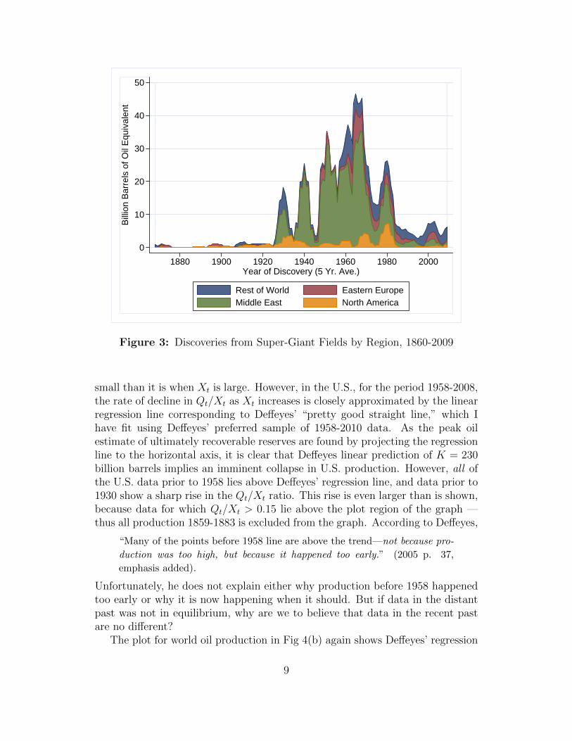
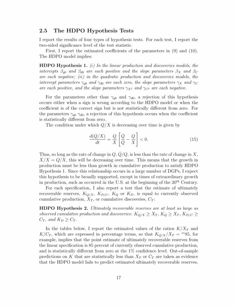
Deffeyes (2005) also produces a graph of what he calls ‘hits’ for discoveries ofgiant oil fields (those greater than 100 million barrels of oil equivalent). Figure 3shows the pattern of discoveries for a comparable data set, that of so-called ‘super-giant’ fields (those greater than 500 million barrels of oil equivalent) by regionbased on data from Horn (2003) updated through 2009. These fields togetheraccount for over 60% of world discoveries. World discoveries of supergiant fieldspeaked in the 1960s. But if one looks at North America, there are several peaks.The one in the 1930s corresponds to when the lower-forty-eight U.S. states peaked(cf. Deffeyes, 2005, at p. 138).

7

0

500

1000

1500

Pro

ved

Res

erve

s

0

20

40

60

80

Pro

duct

ion

& D

isco

verie

s

1950 1960 1970 1980 1990 2000 2010Year

World Production (Billion Barrels)World Discoveries (Five Year Average) (Billion Barrels)World Proved Reserves (Billion Barrels)

Figure 2: Time Paths World Crude Oil Production, Discoveries and Proved Reserves, 1948-2010

2.2 The HDPO Linear Empirical Specification

Since Xt and Ct are each increasing over time, the quadratic versions of theHDPO model, (2) and (4), are estimated on graphs similar to those Figs. 1-3.But Deffeyes uses the the linear relationship given in (1) and (3) to produceestimates of ultimately recoverable reserves.

Fig. 4 shows the relationship between Qt/Xt and Xt using annual data fromU.S. and world crude oil production, respectively, and Fig. 5 shows the corre-sponding plots of Dt/Ct and Ct for U.S. and world oil discoveries. The horizontalaxis is the cumulative production, Xt, in Fig. 4 and cumulative discoveries, Ct,in Fig. 5, each measured in billions of barrels of oil produced. The vertical axisis the ratio Qt/Xt in Fig. 4 and Dt/Ct in Fig. 5. The units of this ratio are 1/tsince both Qt and Dt are barrels per year while Xt and Ct are measured in ofbarrels. Observations at each decade are marked with the year. Both time andcumulative production (discoveries) are rising moving from left to right.

Several important features appear in the U.S. production data shown in Fig.4. First, on average, the ratio Qt/Xt has been declining as Xt rises. Second,the data show that the relationship between Qt/Xt and Xt is is highly nonlinear.That is, the rate of decline in Qt/Xt relative to Xt is much greater when Xt is

8

0

10

20

30

40

50

Bill

ion

Bar

rels

of O

il E

quiv

alen

t

1880 1900 1920 1940 1960 1980 2000Year of Discovery (5 Yr. Ave.)

Rest of World Eastern EuropeMiddle East North America

Figure 3: Discoveries from Super-Giant Fields by Region, 1860-2009

small than it is when Xt is large. However, in the U.S., for the period 1958-2008,the rate of decline in Qt/Xt as Xt increases is closely approximated by the linearregression line corresponding to Deffeyes’ “pretty good straight line,” which Ihave fit using Deffeyes’ preferred sample of 1958-2010 data. As the peak oilestimate of ultimately recoverable reserves are found by projecting the regressionline to the horizontal axis, it is clear that Deffeyes linear prediction of K = 230billion barrels implies an imminent collapse in U.S. production. However, all ofthe U.S. data prior to 1958 lies above Deffeyes’ regression line, and data prior to1930 show a sharp rise in the Qt/Xt ratio. This rise is even larger than is shown,because data for which Qt/Xt > 0.15 lie above the plot region of the graph —thus all production 1859-1883 is excluded from the graph. According to Deffeyes,

“Many of the points before 1958 line are above the trend—not because pro-

duction was too high, but because it happened too early.” (2005 p. 37,

emphasis added).

Unfortunately, he does not explain either why production before 1958 happenedtoo early or why it is now happening when it should. But if data in the distantpast was not in equilibrium, why are we to believe that data in the recent pastare no different?

The plot for world oil production in Fig 4(b) again shows Deffeyes’ regression

9

line—this time estimated using his preferred sample of 1983 forward. The plotof world production is decidedly less linear than the graph of U.S. productionin Fig. 4(a), but it too shows a tendency for all of the data before Deffeyes’preferred sample to lie above the linear regression line, and for values of Qt/Xt

prior to 1930 to increase asymptotically.The exclusion of data which does not fit their theory is central to the Hubbert-

Deffeyes peak oil model. Hubbert (1956), when making his prediction that U.S.production would peak around 1970, omitted all production data prior to 1930.(He never states this explicitly, but any regression using data prior to 1930 resultsin an estimated value of ultimately recoverable reserves, K, that is substantiallylower than 170 billion barrels, which implies an earlier predicted date of the peak.)Thus, to predict the peak in U.S. production in 1970 Hubbert used data between1930 and 1960, excluding the 70% of production data before 1930. To predictU.S. ultimately recoverable reserves, Deffeyes uses data from 1958 forward, ex-cluding the hundred years of data before 1958 (66%). Ironically, Deffeyes, whenestimating K, omits the 1930-1960 data upon which the central claim to scientificprediction – the peak in U.S. production in 1970 – that the HDPO model rests.

To see the problems this causes, I simultaneously estimate the HDPO modelfor the two U.S. samples, using a dummy variable, Z1960, whose value is zerobefore 1960 and one after 1960, to allow for different intercept and slope estimatesacross the samples. The regression results (with Newey-West lag 5 standarderrors in parentheses) and reserves in trillions (1012) of barrels is

Qt/Xt = .0692(.0017)

− .4171(.0415)

Xt − .0112(.0023)

Z1960 + .1615(.043)

Z1960Xt

The F -statistic on the test that Hubbert’s estimate of ultimately recoverablereserves, K = .0692/.4171 = 165.9 billion (109) barrels, is equal to Deffeyes’estimate of K = (.0692 − .0112)/(.4171 − .1615) = 226.9 billion (109) barrels,is F (1, 74) = 22.19, which has a p-value less than 0.01. Thus the data rejectthat Deffeyes’ and Hubbert’s predictions of ultimately recoverable reserves forthe U.S. are the same.13 Furthermore, when estimating the HDPO model forthe world, Deffeyes not only excludes Hubbert’s data, but he also excludes thetwenty-three years before 1983 as well. While the normal scientific method is torefine a theory to explain the data, Hubbert and Deffeyes refine the data to fittheir theory.

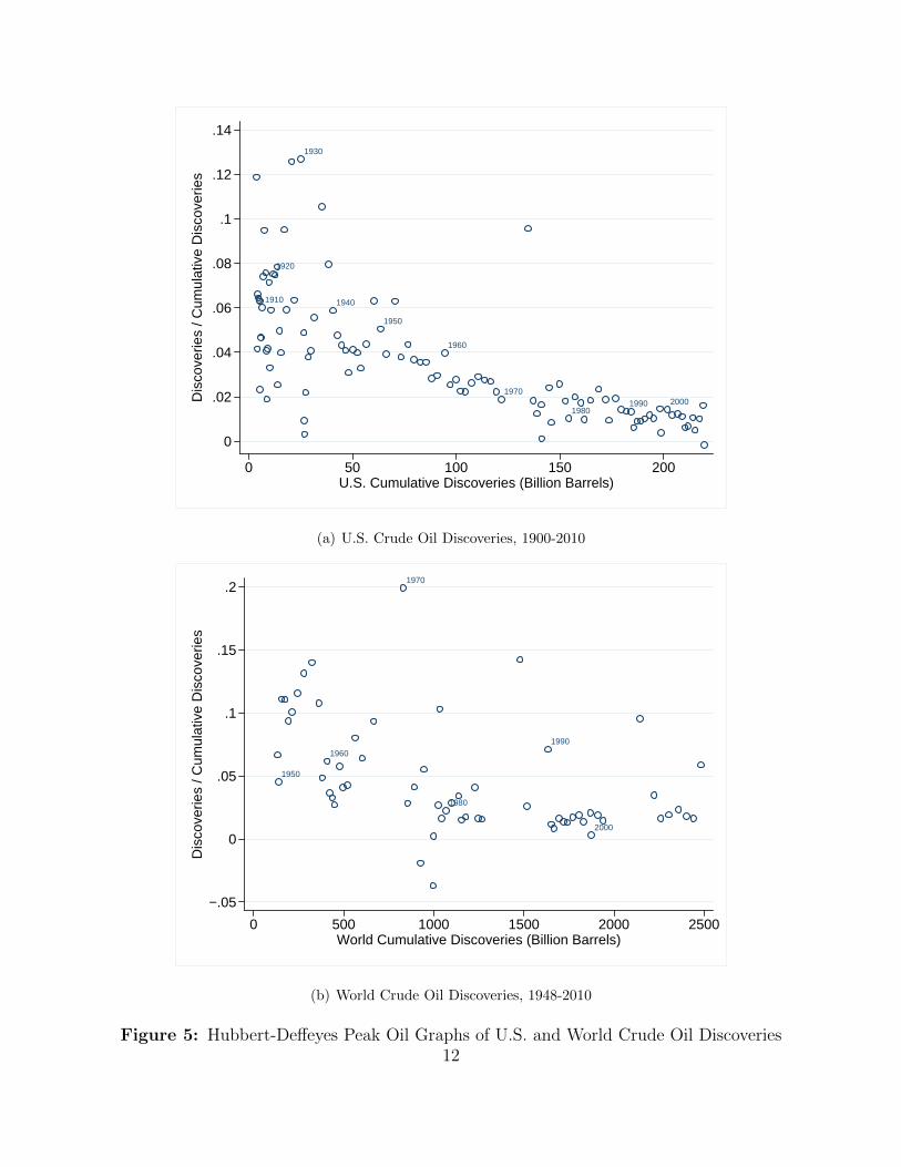
Fig. 5 shows the peak oil analysis of crude oil discoveries for the U.S., 1900-2008, and for the world, 1948-2008, the full periods for which the data are avail-able. Unlike the production data, I do not include a regression line for this dataas Deffeyes does not report an estimate from this data. The discoveries data

13These results are robust to splitting the sample anywhere between 1956 and 1960.

10

1890

1900

1910

1920

1930

1940

1950

19601970

1980

19902000

0

.02

.04

.06

.08

.1

.12

Pro

duct

ion

/ Cum

ulat

ive

Pro

duct

ion

0 50 100 150 200U.S. Cumulative Production (Billion Barrels)

Production / Cumulative ProductionOLS Fitted Values, 1958−2010 Sample

(a) U.S. Crude Oil Production, 1883-2010

1890

1900

19101920

1930

194019501960

1970

1980

1990

2000

0

.02

.04

.06

.08

.1

.12

.14

Pro

duct

ion

/ Cum

ulat

ive

Pro

duct

ion

0 200 400 600 800 1000World Cumulative Production (Billion Barrels)

Production / Cumulative ProductionOLS Fitted Values, 1983−2010 Sample

(b) World Crude Oil Production, 1883-2010

Figure 4: Hubbert-Deffeyes Peak Oil Graphs of U.S. and World Crude Oil Production11

1910

1920

1930

1940

1950

1960

1970

19801990 2000

0

.02

.04

.06

.08

.1

.12

.14

Dis

cove

ries

/ Cum

ulat

ive

Dis

cove

ries

0 50 100 150 200U.S. Cumulative Discoveries (Billion Barrels)

(a) U.S. Crude Oil Discoveries, 1900-2010

1950

1960

1970

1980

1990

2000

−.05

0

.05

.1

.15

.2

Dis

cove

ries

/ Cum

ulat

ive

Dis

cove

ries

0 500 1000 1500 2000 2500World Cumulative Discoveries (Billion Barrels)

(b) World Crude Oil Discoveries, 1948-2010

Figure 5: Hubbert-Deffeyes Peak Oil Graphs of U.S. and World Crude Oil Discoveries12

1900

1920

1940

1960

1980 2000

0

.1

.2

.3

.4

Dis

cove

ries

/ Cum

ulat

ive

Dis

cove

ries

0 500 1000 1500 2000 2500Giant Field Cumulative Discoveries (Billion Barrels of Oil Equivalent)

Figure 6: Hubbert-Deffeyes Peak Oil Graph of World Giant Field Discoveries

exhibit much greater variance than the production data in Fig. 4. Fig. 5(a)shows that the addition of the 9 billion barrel Prudhoe Bay field in 1971 equalledalmost 10% of U.S. discoveries to that point, and that the 1930 discovery of theEast Texas field accounted for an even larger share of cumulative discoveries tothat date. In Fig. 5(b), there are 13 years since 1948 in which current worlddiscoveries were greater than 9% of cumulative discoveries to that date. In addi-tion, there are also two years (1973 and 1975) in which world net discoveries arenegative due to downward revisions of prior estimates of proved reserves.14

As with the production data, there is a negative correlation between the ratioof discoveries-to-cumulative-discoveries, Dt/Ct, and cumulative discoveries, Ct,as is implied by the peak oil model. But, like the production data, the Dt/Ctratio also appears to have a ‘kink’ around 1930 in the U.S. data, although the kinkis less distinct than with the production data. Data on world discoveries doesnot extend back into the 1930s, so whether such a kink exists is indeterminate.

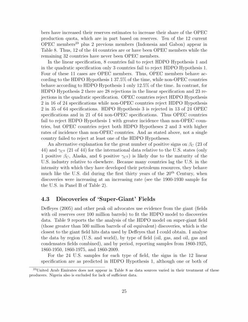
A kink is observed, however, in the super giant field discoveries data in Fig.

14In 1973 and 1975, net world discoveries, calculated from proved reserve changes, are negative becausedownward revisions of previous discoveries were larger than claimed new discoveries in those years. Thereis no instance where this happened with U.S. aggregate discoveries, however, every state and every othercountry experienced negative net discoveries in at least one year when discoveries are calculated from provedreserves.

13

6. The super giant field data differs from the U.S. and world discoveries datain Fig. 5 in three ways. First, the super giant fields data uses 2009 estimatesof reserves for each field from Horn (2003, as updated), attributing all of thereserves subsequently determined to be on the field to the year in which thefield was discovered. As field reserve data are most often revised upwards (e.g.,Maugeri (2009), Nehring (2006b,a,c)), a discovery in the super giant fields datainclude all subsequent revisions as occurring in the year of discovery, while forthe data in Fig. 5, the revisions are added in the year the revisions are made.Second, the super giant fields data include only discoveries in which the fieldhas greater than 500 million barrels of oil equivalent. Third, the super giantfields data include natural gas and condensate fields, converting these into oilequivalent units, while the discoveries data in Fig. 5 contains only data on oiland condensate fields.

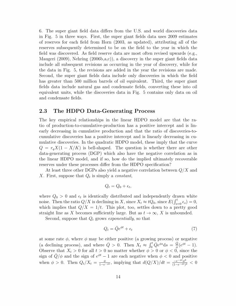
2.3 The HDPO Data-Generating Process

The key empirical relationships in the linear HDPO model are that the ra-tio of production-to-cumulative-production has a positive intercept and is lin-early decreasing in cumulative production and that the ratio of discoveries-to-cumulative discoveries has a positive intercept and is linearly decreasing in cu-mulative discoveries. In the quadratic HDPO model, these imply that the curveQ = rqX(1 − X/K) is bell-shaped. The question is whether there are otherdata-generating process (DGP) which also have the negative correlation as inthe linear HDPO model, and if so, how do the implied ultimately recoverablereserves under these processes differ from the HDPO specification?

At least three other DGPs also yield a negative correlation between Q/X andX. First, suppose that Qt is simply a constant,

Qt = Q0 + εt,

where Q0 > 0 and εt is identically distributed and independently drawn whitenoise. Then the ratio Q/X is declining in X, since Xt ≈ tQ0, since E(

∫ ts=0

εs) = 0,which implies that Q/X = 1/t. This plot, too, settles down to a pretty goodstraight line as X becomes sufficiently large. But as t→∞, X is unbounded.

Second, suppose that Qt grows exponentially, so that

Qt = Qeφt + εt (7)

at some rate φ, where φ may be either positive (a growing process) or negative

(a declining process), and where Q > 0. Then Xt ≈∫ t

0Qeφsds = Q

φ(eφt − 1).

Observe that Xt > 0 for all t > 0 no matter whether φ > 0 or φ < 0, since thesign of Q/φ and the sign of eφt − 1 are each negative when φ < 0 and positive

when φ > 0. Then Qt/Xt = φ1−e−φt , implying that d(Q/X)/dt = −e−φtφ2

(1−e−φt)2 < 0

14

and that dX/dt = Q > 0. Thus, plotting Q/X against X again results in anegative correlation. However, Q/X grows without bound as X → 0.15

Third, suppose that Qt grows according to a geometric function, so that

Qt = tθ + εt, (8)

for θ > −1, where Qt is increasing when θ > 0 and is decreasing when θ < 0. Inthis case, for X(1) = 1/(1+θ), Xt ≈ t(1+θ)/(1+θ), and Qt/Xt = (1+θ)/t. Thus,Xt is increasing over time and Qt/Xt is decreasing over time at a decreasingrate. Therefore, plotting Q/X against X again results in a negative correlation.Again, Q/X grows without bound as X → 0.

Each of these alternative DGP’s have the property that the ratio Q/X is de-creasing in X, so each are capable of generating plots similar to those in Figs.4 and 6. Indeed, each of these, in contrast to the HDPO process, also is con-sistent with the rise in Q/X as X → 0. But each of these DGP has a verydifferent relationship between Q and X as well. With the constant function, Qis independent of X, and with the exponential or geometric DGP, Q is eitherincreasing or deceasing in X. The linear HDPO DGP, therefore, could be forcedto fit data produced by other DGPs with sufficient refinement of the data sam-ple, but these other DGPs have very different implications regarding ultimatelyrecoverable reserves. Furthermore, it is clear that determining which of these fitsthe data requires looking at both the relationship between Q/X and X and therelationship between Q and X.

2.4 Estimation of the HDPO Model

If the linear specifications in (1) and (3) correctly model the discovery and produc-tion process, then by adding white noise errors, εqt and εdt, to the specificationswith Qt/Xt and Dt/Ct as the dependent variables and with Xt and Ct as thesingle regressor, each equation can be estimated as follows:

Qt/Xt = βq0 + βXXt + εqt (9)

Dt/Ct = βq0 + βCCt + εdt, (10)

where βi0 = ri, βX = rq/K, βC = rd/K and εit are statistical residuals, i = q, d.The estimate of K from each equation is

KQ/X = −βq0/βX , and KD/C = −βd0/βC , (11)

15Important economic examples of exponential output equations are the Hotelling (1931) model with lineardemand and constant marginal cost and growth models such as Stiglitz (1974). In both cases, oil productionexponentially declines over time.

15

where βi0, i = q, d, and βX and βC are the estimated coefficients from (9) and(10), and the subscripts on K refer to the dependent variable of the equationfrom this estimate of K is derived. This is the method used in Deffeyes (2003,2005). Throughout, I refer to these as the linear “production” and “discoveries”models, although the dependent variable in each is the ratio of production-to-cumulative-production or discoveries-to-cumulative-discoveries.

An alternative specification of the HDPO model are the quadratic equationsin (2) and (4). These equations can be estimated as follows:

Qt = γq0 + γXXt + γX2(Xt)2 + νqt (12)

Dt = γd0 + γCCt + γC2(Ct)2 + νdt, (13)

where νqt and νdt are the unexplained residuals. In this specification, the depen-dent variable is production and discoveries. The parameters estimates in thisspecification have the interpretations that γX = βq0 = rq, γX2 = βX = rq/K,γC = βd0 = rd and γC2 = βC = rd/K. In addition, the parameters γq0 and γd0

are each zero in the quadratic HDPO model. Thus, one advantage of this spec-ification is that the additional test of the hypotheses that γq0 = 0 and γd0 = 0occurs.

One other feature of the quadratic specification is of note. The estimate of Kis the solution to a quadratic equation:

KQ =−γX2γX2

± 1

2γX2

√γ2X − 4γq0γX2 ,

KD =−γC2γC2

± 1

2γC2

√γ2C − 4γd0γC2 .

(14)

Thus, one problem with this specification is that KQ or KD may be an imaginarynumber.

The models in (9), (10), (12) and (13) are estimated using annual data. Cu-mulative production and cumulative discoveries are based on January 1 esti-mates in year t, while production and discoveries are those that occur January1-December 31 in year t. Because the data is highly autocorrelated across timeand perhaps subject to unknown heteroskedasticity, the models are estimated us-ing the Newey-West (Bartlett kernel) estimator, with a bandwidth of five. Thisestimator provides point estimates of the slope and intercept parameters whichare identical to those from ordinary least squares, but the standard errors forthese estimates are robust for arbitrary heteroskedasticity and up to fifth orderautocorrelation. One asterisk indicates statistical significance at the five percentconfidence level (‘*’) and two asterisks indicates statistical significance at the onepercent confidence level (‘**’).

16

2.5 The HDPO Hypothesis Tests

I report the results of four types of hypothesis tests. For each test, I report thetwo-sided significance level of the test statistic.

First, I report the estimated coefficients of the parameters in (9) and (10).The HDPO model implies:

HDPO Hypothesis 1. (i) In the linear production and discoveries models, theintercepts βq0 and βd0 are each positive and the slope parameters βX and βCare each negative; (ii) in the quadratic production and discoveries models, theintercept parameters γq0 and γd0 are each zero, the slope parameters γX and γCare each positive, and the slope parameters γX2 and γC2 are each negative.

For the parameters other than γq0 and γd0, a rejection of this hypothesisoccurs either when a sign is wrong according to the HDPO model or when thecoefficient is of the correct sign but is not statistically different from zero. Forthe parameters γq0 γd0, a rejection of this hypothesis occurs when the coefficientis statistically different from zero.

The condition under which Q/X is decreasing over time is given by

d(Q/X)

dt=Q

X

[Q

Q− Q

X

]< 0. (15)

Thus, so long as the rate of change in Q, Q/Q, is less than the rate of change in X,X/X = Q/X, this will be decreasing over time. This means that the growth inproduction must be less than growth in cumulative production to satisfy HDPOHypothesis 1. Since this relationship occurs in a large number of DGPs, I expectthis hypothesis to be broadly supported, except in times of extraordinary growthin production, such as occurred in the U.S. at the beginning of the 20th Century.

For each specification, I also report a test that the estimate of ultimatelyrecoverable reserves, KQ/X , KD/C , KQ or KD, is equal to currently observedcumulative production, XT , or cumulative discoveries, CT :

HDPO Hypothesis 2. Ultimately recoverable reserves are at least as large asobserved cumulative production and discoveries: KQ/X ≥ XT , KQ ≥ XT , KD/C ≥CT , and KD ≥ CT .

In the tables below, I report the estimated values of the ratios K/XT andK/CT , which are expressed in percentage terms, so that KQ/X/XT = ∗∗85, forexample, implies that the point estimate of ultimately recoverable reserves fromthe linear specification is 85 percent of currently observed cumulative production,and is statistically different from zero at the 1% confidence level. Out-of-samplepredictions on K that are statistically less than XT or CT are taken as evidencethat the HDPO model fails to predict estimated ultimately recoverable reserves,

17

since ultimately recoverable reserves are at least as great as cumulative produc-tion or discoveries. While the linear models always produce a value of K exceptwhen the slope coefficient is exactly zero, the quadratic models may not predict avalue of K at all if the estimate of K is an imaginary number. Failure to producea value of K is also interpreted as a rejection of HDPO Hypothesis 2.

Third, the HDPO model predicts that the linear relationships in (1) and (3)or the quadratic relationships in (2) and (4) capture the essential features of thedata. The simplest test of this hypothesis is the following:

HDPO Hypothesis 3. The inclusion of higher powers of Xt or Ct, into thelinear or quadratic production and discoveries models has no statistical effect.

For each linear regression, I report the test statistic and its statistical signif-icance for the test of the null hypothesis that βX2 = 0 in the augmented linearproduction model, Qt/Xt = βq0 + βXXt + βX2X2

t + εqt, or that βC2 = 0 in theaugmented linear discoveries model, Dt/Ct = βd0 + βCCt + βC2C2

t + εdt. Thistests whether the linear specification is rejected for each sample. Similarly, foreach quadratic specification, I report a test of the hypothesis that γX3 = 0 inin the quadratic production model, Qt = γq0 + γXXt + γX2(Xt)

2 + γX3X3 + νqt,and a test of the hypothesis that γC3 = 0 in the quadratic discoveries model,Dt = γd0 + γCCt + γC2(Ct)

2 + γC3C3 + νdt. These tests do not exhaust the uni-verse of possible alternative models to the HDPO model, but a rejection of thenull hypothesis is taken as evidence that the HDPO model is misspecified.

Fourth, I also report several cross-equation tests between the quadratic andlinear specifications and between the production and discoveries models:

HDPO Hypothesis 4. (i) The linear and quadratic regression parameters areequal: β0 = γX and βX = γX2 in the production models and β0 = γC and βC = γC2

in the discovery models; (ii) the linear and quadratic regression estimates ofultimately recoverable reserves are equal: KQ/X = KQ and KD/C = KD; and (iii)the estimates of ultimately recoverable reserves are equal across discoveries andproduction specifications of the linear and quadratic regressions: KQ/X = KD/C

in the linear specification and KQ = KD in the quadratic specification.

The cross-equation hypotheses are tested using seemingly-unrelated regressionmethodology, which estimates the the different specifications simultaneously.16

These hypothesis form the empirical basis for evaluating the HDPO model.

16Due to a limitation in Stata’s sureg program, however, these estimates are not corrected for autocorre-lation or heteroskedasticity, as are the Newey-West estimates reported elsewhere. Thus, the tests of HDPOHypotheses 1-3, these test statistics are based on inefficient estimators.

18

3 Analysis of the HDPO Model Using Produc-

tion Data

I now turn to the empirical analysis. Because most of the peak oil estimates areabout U.S. and world crude oil production, I begin with that data.

3.1 Crude Oil Production from the U.S. and World

Table 1 presents the results for the HDPO production model using U.S. andworld crude oil production data on samples ending in 2010: 1859-2010, 1900-2010, 1931-2010, 1958-2010, and 1983-2010. The 1931 break is approximatelywhere the ‘kink’ in the U.S. Q/X graph occurs; 1958 is the first year in Deffeyes’HDPO model fit for U.S. data, while 1983 is the first year Deffeyes chooses tofit the HDPO model using world data. This analysis examines how the sampleselections chosen by Hubbert and Deffeyes affect their estimates of ultimatelyrecoverable reserves. Reported are both the linear and quadratic HDPO models.

In the linear specifications, the predictions of HDPO Hypothesis 1 are foundto occur and to be statistically different from zero in all ten samples. In thequadratic specifications, however, nine out of ten samples have a positive inter-cept, and in the 1983-2010 samples for both the U.S. and the world, the estimatedslope coefficients have the wrong signs according to the HDPO model and 3 outof 4 are statistically significant. Regarding HDPO Hypothesis 2, only the U.S.linear sample beginning in 1859 produces an estimate of KQ/X that is statisticallyless than X2010. In the quadratic specification, however, the samples starting in1983 for both the U.S. and the world cannot produce an estimate of KQ, since thepoint estimates result in an imaginary number. HDPO Hypothesis 3 is rejectedin 8 of 10 samples. HDPO Hypothesis 4 is rejected for all 10 samples.

A supporter of the HDPO model might be satisfied with the U.S. K predic-tions 7 to 17% above current cumulative production and with the world pre-dictions of additional output of between 20 to 111% above current cumulativeproduction. But there should be concern in the 80% rejection rate of HDPOHypothesis 3, that 90% of the quadratic samples rejected a zero intercept, andthat both components of HDPO Hypothesis 4 are rejected in every sample.

Next, let us consider how the HDPO model does when forced to predict out-of-sample. Table 2 presents results for the HDPO production model using U.S.and world crude oil production data on samples which begin in 1859 in Panel A,and in 1900 in Panel B. In panel A the sample periods are 1859-1899, 1859-1930,1859-1960, and 1859-1990, while in Panel B the four sample periods anchoredinstead at 1900.17

17The 1859-2008 and 1900-2008 samples in Table 1 are repeated in Panels A and B, respectively, of Table2 to see the effect of changing samples.

19

In the linear specification, only the 1900-1930 U.S. and world samples rejectHDPO Hypothesis 1. In the quadratic specification, the slope parameters rejectHDPO Hypothesis 1 in 6 of 18 samples, including all samples ending in 1930 andfor the world also the samples ending in 1960. Rejection of HDPO Hypothesis1 is expected only during times of extraordinary expansion of production. Thisclearly is the case during 1900-1930, where U.S. production rose from 63 millionbarrels in 1900 to just over a billion barrels in 1929, a thirteen-fold increase inthree decades (9% average annual growth). Similarly, world production increasedten-fold over this period. In the quadratic specifications, the parameter γ0, whichis expected to be zero by HDPO Hypothesis 1 are found to be different from zeroin 80% of the samples. Regarding HDPO Hypothesis 2, in the linear specification,8 of 10 samples ending 1960 or earlier and 3 of 4 samples ending in 1990 predictthat K is less than or equal to cumulative production in 2010 for both the U.S.and the world. Similarly, in the quadratic specification, 4 of 5 samples endingin 1960 or earlier for the U.S. and 5 of 7 samples ending in 1990 or earlier forthe world predict that K is less than cumulative production in 2010. HDPOHypothesis 3 is rejected in all of the linear specification samples and in 8 of 10of the quadratic samples starting in 1859, and in 9 of 15 linear and quadraticsamples beginning in 1900. HDPO Hypothesis 4 is rejected in every sample aswell.

The rejection of HDPO Hypothesis 2 that K ≥ XT in 21 of 28 samples ending1990 or earlier, and the rejection of HDPO Hypothesis 4 that KQ/X = KQ in11 of 18 samples overall suggests that the HDPO model does poorly predictingout-of-sample. Furthermore, considering the four HDPO Hypotheses together,in Tables 1 and 2 together, not one of the 56 samples satisfies all four HDPOhypotheses.

3.2 Crude Oil Production from 24 U.S. States and 44Countries

Tables 3 and 4 report the estimates of the HDPO model on crude oil productionfor 24 U.S. states and 44 countries, respectively. For each state or country,regressions using the linear and quadratic specifications are run using all availabledata from 1859 to 1972 to estimate ultimately recoverable reserves.18 For eachspecification, the results of the three HDPO Hypothesis tests are reported, whereXT in HDPO Hypothesis 2 is cumulative production through the year 2008. Alsoreported are cumulative production through 2008, and whether the country hasever been a member of OPEC. For those countries (no states had this issue) forwhich production began in the 1970s or later, out-of-sample predictions are basedon data through a later year such as 1990. I exclude all Eastern bloc countries

18The year 1972 is generally believed to be the last year in which the U.S. government-run prorationingcartel remained the major influence over world oil prices.

20

for whom no separate production data existed prior to the break-up of the SovietUnion in 1991, to ensure that the out-of-sample prediction is at least 20 yearsinto the future.

In the linear specifications, no state or country yields parameter point esti-mates that are incorrect in sign relative to the prediction in HDPO Hypothesis1. However, 18 of 24 states and 23 of 44 countries have one or more coefficientswhich are not statistically different from zero. In the quadratic specifications,the intercept, γq0, is statistically different from zero in 10 of 24 states and in 21of 44 countries, and while one or both of the γX and γX2 coefficients are eitherincorrect in sign or statistically insignificant in 4 out of 24 U.S. states and in 21of the 44 countries the γX and γX2 coefficients that are either incorrect in sign orstatistically insignificant. Overall, many more states and countries than expectedreject HDPO Hypothesis 1.

In the linear specification, all 24 U.S. states and all but 4 of the 44 countrieshave an out-of-sample prediction that rejects the null of HDPO Hypothesis 2that K ≥ XT in favor of the alternative hypothesis that K < XT , and not onestate or country produces an out-of-sample prediction of K which is in excessof XT . In 7 countries, furthermore, the estimate of K is positive only becauseboth coefficients are incorrect in sign. In the quadratic specifications, 11 of 24states produce an estimate of K that is statistically less than XT , although one(Ohio) is based on both coefficients being incorrect in sign. For the U.S., onlyArkansas produces an imaginary number estimate of K, but this occurs for sixcountries (Burma, Ecuador, India, Mexico, Oman and Syria). In the quadraticspecification 36 of 44 countries produce an estimate of K which is less thanobserved cumulative production, XT , in 2008, or is an imaginary number. Thus,the HDPO model fails to produce reasonable out-of-sample estimates of K in 37of 48 U.S. states and in 76 of 88 countries.

In the linear specification, 9 of 24 U.S. states and 23 of 44 countries rejectthe null of HDPO Hypothesis 3, and in the quadratic specification, 18 of 24 U.S.states and 18 of 44 countries reject the null. HDPO Hypothesis 4 is also soundlyrejected: 19 of 24 states and 33 of 44 countries reject the null that of KQ/X = KQ,and only two states (Arkansas and Pennsylvania) and one country (Congo) failto reject the null hypothesis that the estimated coefficients are equal in the linearand quadratic specifications, but both states reject that γ0 = 0.

In the linear specification, none of the 24 states or 44 countries fails to rejectone or more of the HDPO Hypotheses, and in the quadratic specification, onlyIllinois and New Zealand fail to reject at least one of the HDPO Hypotheses.Thus, the disaggregated data offer even less support for the HDPO model thandoes the aggregated data reported in Table 1.

21

3.3 Crude Oil Production from 15 U.S. Oil Fields

The concept of a peak in production arose from observations on the time pathsof field production, where fields like Spindletop in Texas were so over drilled thatproduction began to decline after the second year. Thus, I now turn in Table 5to an analysis of 15 U.S. fields which combine production data from 1913-1952published in Zimmermann (1957) with data from 1979-1998 on U.S. fields over100 million barrels in size from the Oil and Gas Journal.19 Production databetween 1913 and 1952 is used to estimate the HDPO model and to estimateK, and the latter is compared with observed cumulative output through 1998.This test is in the spirit of Nehring (2006a,b,c) and Maugeri (2009), who eachexamined production from specific fields and basins in Texas and California.

The estimates of the HDPO parameters in the linear specification reveal thatin only 6 of the 15 fields do both regression parameter estimates satisfy HDPOHypothesis 1, although all point estimates are of the HDPO expected sign. In thequadratic specification, only 3 of 15 fields satisfy all three requirements of HDPOHypothesis 1 (i.e., that γ0 = 0, γX > 0 and γX2 < 0), and for the Haynesville fieldthe signs on the slope coefficients are statistically significant and incorrect. Thus,HDPO Hypothesis 1 is rejected in 21 of 30 specifications. HDPO Hypothesis 2 isrejected by 14 fields in the linear specification and by 13 fields in the quadraticspecification, with only the Homer field in Louisiana producing an estimate of Kthat is greater than observed cumulative production through 1998. In addition,HDPO Hypothesis 3 is rejected in 11 of the linear specifications and in 12 of thequadratic specifications, including the Homer field. Thus, not one of the fieldsfails to reject one or more of HDPO Hypotheses 1-4. Therefore, the field levelanalysis of the HDPO model reveals the same problems as observed at higheraggregations: a forcing of a linear model onto inherently non-linear data.20

4 Analysis of the HDPO Model Using Discov-

eries Data

This section reports tests of the HDPO model hypotheses using discoveries data. Ibegin with discoveries data based on contemporary estimates of proved reservesat first for the U.S. and the world and then for a number of U.S. states andinternational countries, and then examine discoveries data on super-giant fieldswhich uses 2009 estimates of reserves on each field rather than the estimates atthe time of discovery.

Discoveries data from proved reserves are calculated as the change in cumu-lative discoveries, Dt = Ct − Ct−1, where cumuative discoveries are the sum of

19See the Oil and Gas Journal, “Forecast and Review” issue. This data was discontinued after 1998.20These results also suggest that increases in production came from improvements to technology, since the

median HDPO K from data 1913-1952 was about 30% of actual production through 1998.

22

cumulative production and proved reserves, Ct = Xt + Rt. Peak oil advocatestypically ignore this data, preferring to discuss only the data on giant fields. Theyargue that OPEC countries have an incentive to overstate reserves since produc-tion quotas are based on reserves, and that the discoveries data from provedreserves is too noisy.21 There are, however, at least two reasons to consider thisdata. First, as the same level of ultimately recoverable reserves underlies boththe discovery and the production processes in the HDPO model, it interesting tosee if the discoveries data produces a similar estimate of ultimately recoverablereserves as does the production data and whether the same problems as thoseidentified for production data arises when using discoveries data. Second, as bothproduction and exploration decisions in every year are based upon current knowl-edge, this data allows one to estimate the production and discoveries equationssimultaneously.

4.1 Crude Oil Discoveries from the U.S. and World

Table 6 reports the analysis of the HDPO model on U.S. and world discoveries.Panel A reports samples ending in 2010 while panel B reports samples beginningin 1900 for the U.S. and in 1948 for the world. In each case, a linear and quadraticspecification is estimated.

As with the production data, only 4 of 14 linear specification samples rejectHDPO Hypothesis 1. In the quadratic specifications, however, 9 of 14 samples,all 6 of the world samples and 3 of 8 U.S. samples, reject HDPO Hypothesis 1.Thus one or more components of HDPO Hypothesis 1 is rejected in nearly halfthe samples, including Deffeyes’ preferred sample for world production, the 1983-2010 linear sample. For HDPO Hypothesis 2, in only two cases, the 1900-1930U.S. linear specification (for which the estimate of K is negative) and the 1948-1960 world quadratic specification, is the estimated K value less than cumulativediscoveries in 2010. HDPO Hypothesis 3 is rejected in only 6 of 28 samples, 2 byan estimate of K less than CT and 4 by an estimate of K which is an imaginarynumber. For HDPO Hypothesis 4, Table 6 reports both the tests (i) and (ii)between the linear and quadratic discoveries specifications (as in Tables 1 and2) and the tests (iii) between the production and discoveries specifications. Thetests of equality between the linear and quadratic samples show that one or bothof HDPO Hypotheses 4(i) and 4(ii) are rejected in all samples. But for the testsof HDPO Hypotheses 4(iii) between the estimates of K between the productionand discoveries equations, the hypothesis is only rejected for all 12 world samplesand for 3 U.S. quadratic samples for the U.S.. Overall, the discoveries data satisfyHDPO Hypotheses 1-4 in not a single U.S. or world sample.

Interestingly, the point estimate for the linear 1983-2010 world discoveries

21Hubbert (1982), for example, plots U.S. discoveries data with most of the variation removed by presentingonly 11 year averages (Fig. 32, p. 92).

23

sample is over 630% of current estimated world cumulative discoveries (althoughit is not statistically significant). This estimate would imply ultimately recover-able reserves of over fifteen trillion barrels, a number that is more than five timeslarger than any published estimates (Salvador, 2005). One can see why Deffeyesdoes not wish report results of the HDPO model using these data.

4.2 Crude Oil Discoveries from 24 U.S. States and 44Countries

Tables 7 and 8 report the analysis of the HDPO model using discoveries datacalculated from proved reserves data on 24 U.S. states and 44 countries. As withthe production data, the out-of-sample tests are conducted using predictionsof ultimately recoverable reserves based on samples from 1948 to 1972.22 Thisestimate of K is compared to cumulative discoveries at the end of 2010.

For the 24 U.S. states in the linear specification, the signs on the estimatedcoefficients are in agreement with HDPO Hypothesis 1 in all but Alaska and Ohio(where in both cases the point estimate is statistically insignificant), althoughone or more coefficients are statistically insignificant in 9 states. In the quadraticspecification, however, only 4 states (Alabama, Louisiana, Nebraska and NewMexico) have the correct signs and significance levels in accordance with HDPOHypothesis 1. One or both of HDPO Hypothesis 3 are rejected in 16 of 24linear samples and in 21 of 24 quadratic samples. Only in Florida (in the linearspecification) and Louisiana (in both the linear and quadratic specifications)do all of the HDPO Hypotheses 1-3 fail to be rejected. Yet, even Florida andLouisiana reject HDPO Hypothesis 4 that the quadratic and linear specificationsare equal, and only for Alaska and Montana do none of HDPO Hypothesis 4 getrejected.

Of the 44 countries in Table 8, in the linear specification only 8 countries failto reject HDPO Hypothesis 1. Indeed, in 24 of 44 countries, the slope coefficientβC on cumulative discoveries is positive in sign, and in 6 countries (Bahrain,Brunei, Congo, Ecuador, Trinidad & Tobago and the United Kingdom), thepositive coefficient is statistically different from zero. Furthermore, not a singlecountry in either the linear or quadratic specifications fails to reject one or moreof the HDPO hypotheses, and only Canada, Chile and Columbia fail to rejectone or more of HDPO Hypothesis 4.

OPEC Incentives and Analysis of the HDPO Model on DiscoveriesData

Campbell (1997), Deffeyes (2005) and Simmons (2006) argue that OPEC mem-

22While reserves data are available for the U.S. as a whole back to 1900, estimated proved reserve data bystate are only available from 1948.

24

bers have increased their reserves estimates to increase their share of the OPECproduction quota, which are in part based on reserves. Ten of the 12 currentOPEC members23 plus 2 previous members (Indonesia and Gabon) appear inTable 8. Thus, 12 of the 44 countries are or have been OPEC members while theremaining 32 countries have never been OPEC members.

In the linear specification, 8 countries fail to reject HDPO Hypothesis 1 andin the quadratic specification only 3 countries fail to reject HDPO Hypothesis 1.Four of these 11 cases are OPEC members. Thus, OPEC members behave ac-cording to the HDPO Hypothesis 1 37.5% of the time, while non-OPEC countriesbehave according to HDPO Hypothesis 1 only 12.5% of the time. In contrast, forHDPO Hypothesis 2 there are 28 rejections in the linear specification and 23 re-jections in the quadratic specification. OPEC countries reject HDPO Hypothesis2 in 16 of 24 specifications while non-OPEC countries reject HDPO Hypothesis2 in 35 of 64 specifications. HDPO Hypothesis 3 is rejected in 13 of 24 OPECspecifications and in 21 of 64 non-OPEC specifications. Thus OPEC countriesfail to reject HDPO Hypothesis 1 with greater incidence than non-OPEC coun-tries, but OPEC countries reject both HDPO Hypotheses 2 and 3 with higherrates of incidence than non-OPEC countries. And as stated above, not a singlecountry failed to reject at least one of the HDPO Hypotheses.

An alternative explanation for the great number of positive signs on βC (23 of44) and γC2 (21 of 44) for the international data relative to the U.S. states (only1 positive βC , Alaska, and 6 positive γC2) is likely due to the maturity of theU.S. industry relative to elsewhere. Because many countries lag the U.S. in theintensity with which they have developed their petroleum resources, they behavemuch like the U.S. did during the first thirty years of the 20th Century, whendiscoveries were increasing at an increasing rate (see the 1900-1930 sample forthe U.S. in Panel B of Table 2).

4.3 Discoveries of ‘Super-Giant’ Fields

Deffeyes (2005) and other peak oil advocates use evidence from the giant (fieldswith oil reserves over 100 million barrels) to fit the HDPO model to discoveriesdata. Table 9 reports the the analysis of the HDPO model on super-giant field(those greater than 500 million barrels of oil equivalent) discoveries, which is theclosest to the giant field hits data used by Deffeyes that I could obtain. I analysethe data by region (U.S. and world), by type of field (oil, gas, and oil, gas andcondensates fields combined), and by period, reporting samples from 1860-1925,1860-1950, 1860-1975, and 1860-2009.

For the 24 U.S. samples for each type of field, the signs in the 12 linearspecification are as predicted in HDPO Hypothesis 1, although one or both of

23United Arab Emirates does not appear in Table 8 as data sources varied in their treatment of theseproducers. Nigeria also is excluded for lack of sufficient data.

25

the regression coefficient estimates is statistically zero in 3 of 12 U.S. cases. Inthe U.S. quadratic samples, γ0 is statistically different from zero in only one case(1860-1950 sample for all fields) and γC is statistically positive in all samples andγC2 is negative in all samples and statistically different from zero in all but theearliest oil and all fields samples.

For the world samples, the estimated parameter βC in the linear specificationis positive in sign in 5 of 12 cases (and statistically significant in the two earlygas cases) and is statistically insignificant in 6 of 12 cases. In the quadraticspecifications, there are two instances (both for gas fields) where the parameterγ0 is statistically different from zero, and in the 1860-1925 samples, both γC andγC2 are insignificant for oil and all fields and are significant but of the oppositesign predicted by the HDPO model for natural gas fields.

HDPO Hypothesis 2 is rejected for the U.S. for all samples ending on orbefore 1950, for both the linear or quadratic specifications, and for all samplesin the linear specification for natural gas. For the world, 9 of 12 samples endingon or before 1950 for both the linear and quadratic specifications reject HDPOHypothesis 2, but none of the samples in either specification ending after 1950result in a rejection of HDPO Hypothesis 2. HDPO Hypothesis 3 is rejected in thelinear model only for the world in the natural gas samples, but in the quadraticmodel, it is rejected in 9 of 16 cases and occurs in each field type and for boththe U.S. and the world. HDPO Hypotheses 4 can only be tested using the linearversus quadratic specifications, but either the equality of coefficients or equalityof estimated K is rejected in half of the samples, with rejections occurring moreoften in samples using more recent data.

When taken together all 24 U.S. samples reject one or more of the HDPOHypotheses 1-4, and 23 of 24 of the world samples reject one or more of the HDPOHypotheses 1-4. Thus, the results on the HDPO preferred data on discoveriesrejects the HDPO Hypotheses with greater frequency than does the discoveriesdata using contemporary estimates of discoveries reported in Tables 6-8.

5 Peak Everything?

‘Peak Everything?’ is the title of a book by Heinberg (2007), which argues thatfor many resource commodities, consumption is about to peak. In this section, Iconsider the application of the HDPO model to resources other than oil. I beginwith coal, which has been the subject of recent analysis in Heinberg and Fridley(2010), and then turn to a panel of 78 minerals, and finally to a panel of 21agricultural goods. I also use the 78 minerals data, supplemented with data fromcoal and petroleum data, to briefly examine the case by optimists.

26

1770

1780

1790180018101820

18301840

1850

186018701880189019001910

1920

19301940

19501960

1970 1980 19902000

2010

186018701880

18901900

19101920 19301940 1950

19601970

1980

1990 2000

2010

0

2

4

6

8

Wor

ld C

oal P

rodu

ctio

n (B

illio

n M

etric

Ton

s)

0

.02

.04

.06

.08

Pro

duct

ion

/ Cum

ulat

ive

Pro

duct

ion

50 100 150 200 250 300 350World Cumulative Coal Production (Billion Metric Tons)

Production / Cum. Production OLS 1850−1950OLS 1951−2010 World Production

Figure 7: Hubbert-Deffeyes Peak Oil Applied to World Coal Production, 1751-2008

5.1 Coal Production Data

Given the obvious link between Jevon’s (1866) concern about coal in Britain andthe modern concerns of the peak oil literature, coal is a natural place to study thepeak oil model. Coal has also been the subject of peak oil analysis by Hubbert(1956, Fig. 1) and, more recently, by Heinberg and Fridley (2010).

Fig. 7 plots the ratio of production-to-cumulative-production against cumu-lative production for world coal production from 1751.24As with the graphs forcrude oil production in Fig. 4, the ratio Qt/Xt is on average decreasing in cumu-lative production, Xt. As with oil, there also appears to be a ‘kink’ in the plotof Qt/Xt against Xt occurring in approximately 1950.

To an observer like Hubbert (1956) looking at historical coal production datain 1950, at which point about 100 billion (109) metric tons of coal had beenconsumed, and using the HDPO methodology, it might appear that coal wasnearing exhaustion. The downward sloping solid line is the predicted path of

24Coal data for 1981-2010 are from the 2010 BP Statistical Review of World Energy. Coal data from1751-1980 are from Andres et al. (1999), from which I calculated coal production from “Emissions from solidfuel consumption” production using the average conversion of one metric ton of CO2 equaling 0.5 metrictons of coal for the world, 0.55 metric tons of coal for the U.S. and 1 metric ton of coal for the U.K. Thesefactors are the average for the overlap of data from 1981-2006.

27

Qt/Xt as a linear function of Xt based on a regression using data from 1850-1950, which, in keeping with the HDPO methodology, drops about half of theavailable data. This analysis indicates that exhaustion should occur at about155 billion metric tons. Yet cumulative production in 2008 was more than twicethis, at 300 billion metric tons. As can be seen in Fig. 7, cumulative world coalproduction has continued to rise well beyond the estimate based on 1850-1950data. The ratio Qt/Xt flattened out to around 2% of cumulative production,where it has remained. The second flatter dashed line is the regression using1951-2010 data. It is has a much lower slope coefficient, which implies a muchhigher estimate of ultimately recoverable reserves (K = 3, 900 billion metric tons,which is more than twenty-five times larger than the estimate based on 1850-1950data, and is about four and a half times larger than the World Energy Council(2010) estimate of 861 billion tons of recoverable coal reserves).

Comparing the USGS’s estimate of 362 billion barrels of ultimately recoverableU.S. oil to his own estimate of 228 billion barrels, Deffeyes sarcastically remarked,

“Either that straight line is going to make a sudden turn, or the USGS was

counting on bringing in Iraq as the fifty-first state” (2005, p. 36).

What Fig. 7 shows is that the ‘sudden turn’ did occur for coal. The peak oilmodel applied to coal using data 1850-1950 produced an estimate of ultimate coalproduction that was passed only decade or two later. Hubbert did not mentionthis in his 1982 update.

Table 10 analyzes the HDPO model in greater detail for coal data, using threegeographical regions (U.S., U.K., and the world), four sample periods 1751-1850,1751-1900, 1751-1950, and 1751-2010, and a linear and quadratic specificationof the HDPO. For the linear specification, HDPO Hypothesis 1 is rejected dueto an insignificant slope coefficient, βX , 2 of 4 times for the world, 0 of 4 timesfor the U.K., and 1 of 4 times for the U.S. In the quadratic specification, 3 of4 samples for each region reject that γ0 is zero, and in each of the 1741-1850samples, the coefficient γX2 is positive and significant, in contrast to the HDPOmodel. Furthermore, HDPO Hypothesis 2 is rejected in all but the world 1751-2010 sample in the linear specification. In the quadratic specification, HDPOHypothesis 2 is rejected in half of the samples in total, although not for any ofthe samples using the full data from 1751-2010. HDPO Hypothesis 3 is rejectedin only one sample (world, 1751-2010) in the linear specification, and in 7 of 12samples in the quadratic specification. Only the 1751-1900 world sample fails toreject one or more of HDPO Hypothesis 4. Finally, all 24 of the samples rejectat least one of the HDPO Hypotheses.

I conclude by revisiting the British experience with coal. According to Maddi-son (2003), in the nine decades before coal peaked in Britain, from 1820 to 1913,British real per capita GDP rose at an annual rate of 1.14%, while in the ninedecades after coal production peaked in Britain, British real per capita GDProse by an annual rate of 1.63% from 1913 to 2003. Thus, in contrast to the

28

predictions of Jevon, the British did much, much more after coal peaked thanwhat they did before it peaked.

5.2 78 Minerals

Next, I apply the peak oil model to the production paths of 78 other mineralresources. Some of these resources differ from oil in that they are recyclable, andall, like coal, have substantially smaller direct world GDP shares than does crudeoil. Nevertheless, the peak oil model has been applied to other resources in (e.g.,Heinberg, 2007), so it is useful to see whether the problems identified for coaland petroleum also hold in this broader set of minerals.

Tables 11 and 12 report the analysis of the HDPO model on a set of seventy-eight minerals for the period 1900-2008.25 The analysis uses data for the period1900-1950 to estimate the HDPO model and to generate a predicted value of K,which is then compared to the observed cumulative production through 2008. Inaddition, I also test HDPO Hypothesis 3.

For the linear specifications, HDPO Hypothesis 1 is rejected for only 17 of 78minerals, and no instances occur where a sign is incorrect according to the HDPOmodel and is statistically significant. In the quadratic specifications, however, 58of the 78 minerals reject HDPO Hypothesis 1 that γ0 is zero, and there areseveral instances (asbestos, gallium, iron-oxides, mica flake, peat, rhenium, andtalc) where the slope coefficient signs are incorrect according to the HDPO modeland are statistically significant. Indeed, only bromine, cadmium, molybdenum,pumice, and strontium (5 of 78) have the HDPO expected signs and significancefor all three parameters. HDPO Hypothesis 2 is rejected for all 78 minerals inthe linear specification, and in the quadratic specification, K is statistically lessthan XT in 38 of 78 cases and in and additional 25 cases K cannot be calculatedbecause the point estimates yield an imaginary number. HDPO Hypothesis 3is rejected in 62 of 78 cases in the linear specification and in 25 cases (plus onecase, thallium, where the test could not be conducted due to multicollinearity) inthe quadratic specification. Only 6 minerals fail to reject HDPO Hypothesis 4(i)regarding KQ/X = KQ, and only chromium and gravel industrial fail to rejectHDPO Hypothesis 4(ii) that the estimated coefficients are not equal across thequadratic and linear specifications, and for gravel the intercept in the quadraticspecification is statistically different from zero. Not a single mineral satisfies allof HDPO Hypotheses 1-4. This is evidence that the problem of non-linearity inthe peak oil model is not confined to energy resources.

25Data for 76 non-fuel minerals is from Kelly and Matos (2007). Data for natural gas and uranium isfrom the 2009 BP Statistical Review of Energy. Natural gas production is in millions of cubic feet. Uraniumproduction is in millions of pounds. Nuclear electricity production is converted into uranium productionusing the 1994-2006 average rate of 14.36 terra-Watt hours (1012 Watt hours) per million pounds of uraniumcalculated from Energy Information Agency data.

29

5.3 21 Agricultural Commodities

In this section, I show what happens when the HDPO model is applied to datafor which the data generating process is undoubtedly different from the HDPOassumption. With agricultural production, there is no reason to suppose thatcumulative production is bounded at all. In the linear HDPO model, an un-bounded process is identified by a coefficient on cumulative production whichis statistically equal to zero. The precedent for applying the HDPO model tosuch a commodity is Pauly et al. (2003), who have applied the HDPO model tofisheries, which, like agriculture production, are potentially sustainable, so thereis no reason to expect that cumulative agricultural production to be bounded.

Table 13, applies the HDPO model to twenty-one agricultural commodities,using production data for the U.S. based on data in the U.S. Historical Statistics,supplemented by more recent data in the Statistical Abstract of the United Statesto bring the series complete through 2008. I use data between 1800 and 1950 toestimate the HDPO model and then I compare the predicted ultimate cumula-tive production with observed cumulative production through 2008, and to testwhether a higher order terms on cumulative production should be included inthe regressions.

The results are very similar to those in the previous tables. For HDPO Hy-pothesis 1, in the linear specification the coefficient on cumulative production isnegative and statistically different from zero in all twenty-one commodities. Thisimplies that the HDPO model identifies each of these commodities as having anupper bound on production. Since output of every one of these commoditiesexcept wool has been increasing, this casts doubt on the ability of the HDPOmodel to identify a sustainable process. The quadratic specification rejects thatthe intercept is zero for 19 of 21 commodities, and rejects the slope coefficients ashaving the HDPO predicted signs in 11 of 21 cases, including cattle for which thecoefficient on C2

t is positive and significant. For HDPO Hypothesis 2, in the linearspecification the data reject the hypothesis that K = XT in favour of the alterna-tive hypothesis that K < XT in all 21 commodities; in the quadratic specification,however, this only occurs in 8 commodities. In addition, HDPO Hypothesis 3is also rejected in 19 of 21 commodities in the linear specification and in 13 of21 commodities in the quadratic specification. Finally, HDPO Hypotheses 4 arerejected for all 21 commodities. These results imply that the HDPO model isincapable of distinguishing between processes for which cumulative production isfundamentally unbounded and those for which it is bounded.

In short, the non-linearity identified in the petroleum data appear to be amuch more universal truth than is the HDPO assumption that the ratio ofproduction-to-cumulative-production is linearly decreasing in cumulative produc-tion.

30

Aluminum

Antimony

Arsenic

Asbestos

Barite

Bauxite

Beryllium

BismuthBoron

Bromine

Cadmium

Cement

Chromium

Coal

CobaltColumbiumCopper

Diamond

Diatomite

Feldspar

Fluorspar

Gallium

Garnet

Gemstones

Germanium

Gold

GraphiteGravel Construction

Gravel Industrial

Gypsum

Helium

Indium

Iodine

Iron−Ore

Iron−Oxides

Kyanite

Lead Lime

Lithium

Magnesium Compounds

Magnesium Metals

Manganese

Mercury

Mica Flake

Mica Sheet

MolybdenumNatural Gas

Nickel Nitrogen

Peat

Perlite

Petroleum

Phosphate Rock

Platinum

Potash

Pumice

Quartz Crystal

Rare Earth

Rhenium

SaltSelenium

Silicon

Silver

Sodium Carbonate

Sodium Sulfate

Strontium

Sulfur

TalcTantalum

Tellurium

Thallium

Thorium

Tin

Titanium

Tungsten

Uranium

Vanadium

Vermiculite

WollastoniteZinc

Zirconium

−.0

6−

.04

−.0

20

.02

.04

.06

Rea

l Pric

e G

row

th R

ate

0 .02 .04 .06 .08 .1Production Growth Rate

Figure 8: Growth in Real Prices and Quantities, 1900-2007

5.4 The Optimists’ Case

I conclude this section by briefly considering why the HDPO model consistentlyunderestimates potential production. Figure 8 shows the average annual percent-age growth rate in real prices and in output over the period 1900-2008 for the78 mineral commodities from Table 11 plus crude oil and coal production. Twoimportant features stand out in the data presented in Fig. 8. First, real pricesdeclined in 51 of 80 minerals (62%).26 Second, per capita production grew in 62of 80 (78%) minerals, as is indicated in Fig. 8 by observations to the right ofthe vertical line, which corresponds to Maddison’s estimate of world populationannual growth 1950-2003, n = 1.35%. Indeed, in 48 of the 80 minerals (60%),real prices fell while per capita consumption increased.

The only way to get rising output with falling prices is for the supply curve tobe shifting faster than the demand curve. This effect is generally associated withtechnological change. Technological change explains why all of the estimates ofultimately recoverable reserves, including those of peak oil analysts, have been in-creasing over time (Salvador, 2005). Maugeri (2009) provides a specific example:for the Kern River field in California, after producing 278 million barrels since

26This result has been shown for earlier periods by Barnett and Morse (1963) and Slade (1982), amongothers.

31

discovery in 1899, estimates in 1942 were that 54 million barrels of oil remained;yet by 1988, an additional 736 million barrels were produced and estimates ofremaining reserves were raised to 970 million barrels; and today, after producingover 2 billion barrels, estimates are that 627 million barrels remain recoverable.Nehring (2006c) found similar results for the Permian Basin.

6 Conclusions

The Hubbert-Deffeyes peak oil model predicts that world petroleum produc-tion is about to peak and that once this occurs, the pressures of rising pricesand declining production will have profound and serious consequences on theworld economy. While most observers believe that production must eventuallypeak—either because reserves are physically exhausted or because a substitutemakes them economically unviable—the peak oil model claims that this peak isboth imminent and inevitable. Emotionally, the argument is powerful: we havesquandered an endowment millions of years in the making in a brief century anda half. But unlike geological methods of estimating potential oil reserves, theHDPO model relies entirely upon using the historical paths of production anddiscoveries to predict ultimately recoverable reserves.

In this paper I have investigate the empirical robustness of these methods. Iargue that the HDPO model attempts to force a linear relationship onto datawhich are inherently non-linear. The problems this causes manifest themselvesin two ways. First, Hubbert (1956) and Deffeyes (2005) are forced to arguethat historical data of sufficient time in the past is irrelevant for predicting ul-timately recoverable reserves (‘it happened too early’). They are forced to dothis because estimates of future production based on data sufficiently far intothe past produces estimates of ultimately recoverable reserves that are less thanobserved cumulative production, offering an obvious refutation of their hypoth-esis. Second, Campbell (1997), Deffeyes (2005) and Simmons (2006) are forcedto argue that estimates of proved reserves among OPEC countries are overstatedand unreliable. They must argue this in order to defend estimates of ultimatelyrecoverable reserves which are smaller than some estimates of current provedreserves.

I find, however, that the non-linearities in the data undo peak oil model at-tempts to measure ultimately recoverable reserves. This non-linearity causesa plot of the ratio of production-to-cumulative-production against cumulativeproduction to continually become flatter as cumulative production rises. Thus,HDPO estimates of ultimately recoverable reserves made using data more than30 years into the past are incapable of predicting ultimately recoverable reserveseven as large as currently observed cumulative production or discoveries. Fur-thermore, the HDPO specification is shown to produce statistically different re-sults using mathematically equivalent linear and quadratic specifications of the

32

model, and estimates using production and discoveries data yield statisticallydifferent predictions about ultimately recoverable reserves. These problems withthe HDPO model are shown to occur for U.S. and world petroleum productionand discoveries, and for discoveries of super-giant fields, as well as for less aggre-gated production and discoveries data at U.S. states, international countries, andat individual fields levels. Furthermore, these problems are shown to also occurfor data on production from other resources, such as coal and a set of 78 minerals.Finally, I show that the HDPO model is incapable of identifying a data for whichno logical bound exists on cumulative production, by applying the model to 21agricultural commodities, where I find that the HDPO model predicts imminentcollapse of production of these commodities.

While it is clear that oil production might eventually peak, the evidence Ipresent in this paper suggests that the Hubbert-Deffeyes peak oil model haslittle, if anything, to say about either the timing of that eventuality or of themagnitude of ultimately recoverable reserves.

References

American Petroleum Institute, “API Basic Petroleum Data Book,” 2009,(August).

Andres, R. J., D. J. Fielding, G. Marland, T. A. Boden, N. Kumar, andA. T. Kearney, “Carbon dioxide emissions from fossil-fuel use, 1751-1950,”Tellus, 1999, 51, 759–765.

Barnett, Harold J. and Chandler Morse, Scarcity and Growth: The Eco-nomics of Natural Resource Availability, Johns Hopkins University UniversityPress, 1963.

Blanchard, Oliver J. and Jordi Gali, “Macroeconomic Effects of Oil Shocks:Why are the 2000s so Different from the 1970s?,” NBER Working Paper, 2007,(13368).

Bradley, Paul G., “Increasing Scarcity: The Case of Energy Resources,” Amer-ican Economic Review Papers and Proceedings, 1973, 63 (May), 119–125.

Brandt, Adam R., “Testing Hubbert,” Energy Policy, 2006, 35, 3074–3088.

Campbell, Colin, The Coming Oil Crisis, Multi-Science Publishing Company,1997.

Campbell, Colin J. and Jean H. Laherrere, “The End of Cheap Oil,”Scientific American, 1998, (March), 78–83.

33

Considine, Timothy J. and Maurice Dalton, “Peak Oil in a Carbon Con-strained World,” International Review of Environmental and Resource Eco-nomics, 2008, 1 (4), 327–365.

Deffeyes, Kenneth S., Hubbert’s Peak: The Impending World Oil Shortage,Princeton, New Jersey: Princeton University Press, 2003.

, Beyond Oil: The View from Hubbert’s Peak, New York: Hill and Wang, 2005.

Dvir, Eyal and Kenneth S. Rogoff, “Three Epochs of Oil,” NBER WorkingPaper, 2009, (14297).

Fisher, William L., “Can the U.S. Oil and Gas Resource Base Support Sus-tained Production?,” Science, 1987, 236 (26 June), 1631–1636.

Fouquet, Roger and Peter J. G. Pearson, “A Thousand Years of EnergyUse in the United Kingdom,” Energy Journal, 1998, 19 (4), 1–41.

and , “Seven Centuries of Energy Services: The Price and Use of Light inthe United Kingdom,” Energy Journal, 2006, 27 (1), 139–177.

Goodstein, David, Out of Gas: The End of the Age of Oil, New York: W. W.Norton and Company, 2005.

Gordon, H. Scott, “The Economic Theory of a Common-Property Resource:The Fishery,” Journal of Political Economy, 1954, 62, 124–42.

, “Today’s Apocalypses and Yesterday’s,” American Economic Review Papersand Proceedings, 1973, 63 (May), 106–110.

Hall, Charles A. S. and Cutler J. Cleveland, “Petroleum Drilling andProduction in the United States: Yield per Effort and Net Energy Analysis,”Science, 1981, 211 (6 February), 576–579.

Hamilton, James D., “Causes and Consequences of the Oil Shock of 2007-08,”Brookings Papers on Economic Activity, 2009, (Spring), 215–267.

, “Understanding Crude Oil Prices,” Energy Journal, 2009, 30 (2), 179–206.

, “Oil Prices, Exhaustible Resources, and Economic Growth,” NBER WorkingPaper 17759, 2012.

Heinberg, Richard, Peak Everything: Waking Up to the Century of Declines,Garbriola Island, British Columbia: New Society Publishers, 2007.

and David Fridley, “The End of Cheap Coal,” Nature, 2010, 468 (18 Novem-ber), 367–369.

34

Holland, Stephen P., “Modeling Peak Oil,” Energy Journal, 2008, 29 (2), 61–79.

Horn, Myron K., “Giant Fields 1868-2003, Data on a CD-ROM,” in Michel T.Halbouty, ed., Giant Oil and Gas Fields of the Decade 1990-1999, AAPGMemoir 78, Tulsa, Oklahoma: American Association of Petroleum Geologists,2003.

Hotelling, Harold, “The Economics of Exhaustible Resources,” Journal of Po-litical Economy, 1931, (April), 137–175.

Hubbert, M. King, “Nuclear Energy and the Fossil Fuels,” Drilling and Pro-duction Practice, 1956.

, “Techniques of Prediction as Applied to the Production of Oil and Gas,” inSaul I. Gass, ed., Saul I. Gass, ed., 1982.

Jevons, William S., The Coal Question; An Inquiry Concerning the Progress ofthe Nation and the Probable Exhaustion of Our Coal-Mines, London: MacMil-lan And Co., 1866.

Kelly, T.D. and G. R. Matos, “Historical statistics for mineral and materialcommodities in the United States,” U.S. Geological Survey Data Series 140(http://pubs.usgs.gov/ds/2005/140/), 2007.

Kerr, Richard A., “How Much Oil? It Depends on Whom You Ask,” Science,1981, 212 (24 April), 427–429.

, “The Next Oil Crisis Looms Large—And Perhaps Close,” Science, 1998, 281(21 August), 1128–1131.

, “Peak Oil Production May Already Be Here,” Science, 2010, 331 (25 March),1510–1511.

Kilian, Lutz, “Not All Oil Price Shocks Are Alike: Disentangling Demand andSupply Shocks in the Crude Oil Market,” American Economic Review, 2009,99 (June), 1053–1069.

Maddison, Angus, World Economy: Historical Statistics, Paris: DevelopmentCentre of the Organization for Economic Co-operation and Development, 2003.

Malthus, Thomas Robert, An Essay on the Principle of Population, NewYork: Penguin Classics (1970), 1798.

Maugeri, Leonardo, “Squeezing More Oil from the Ground,” Scientific Amer-ican, 2009, (October), 56–63.

35

Meadows, Donella H., Dennis L. Meadows, Jørgen Randers, and W.W.Behrens, III., Limits to Growth 1972.

Mitchel, Brian R., British Historical Statistics, Cambridge, U.K.: CambridgeUniversity Press, 1988.

Nehring, Richard, “How Hubbert Method Fails to Predict Oil Production inthe Permian Basin,” Oil and Gas Journal, 2006, 104 (14), 30–35.

, “Post-Hubbert Challenge is to Find New Methods to Predict Production,EUR,” Oil and Gas Journal, 2006, 104 (16), 43–51.

, “Two Basins Show Hubbert’s Method Underestimates Future Oil Produc-tion,” Oil and Gas Journal, 2006, 104 (13), 37–44.

Nordhaus, William D., “World Dynamics: Measurement without Data,” Eco-nomic Journal, 1973.

, “Resources as a Constraint on Growth,” American Economic Review Papersand Proceedings, 1974, 64 (May), 22–26.

Pauly, Daniel, Jackie Alder, Elena Benett, Villy Christensen, PeterTyedmers, and Reg Watson, “The Future for Fisheries,” Science, 2003,302 (21 November), 1359–1361.

Roberts, Paul, The End of Oil: On the Edge of a Perilous New World, NewYork: Houghton-Mifflin, 2004.

Rosenberg, Nathan, “Innovative Responses to Materials Shortages,” AmericanEconomic Review Papers and Proceedings, 1973, 63 (May), 111–118.

Salvador, Amos, “Energy: A Historical persepective and 21st century forecast,”AAPG Studies in Geology, 2005, 54, 33–121.

Simmons, Matthew R., Twighlight in the Desert: The Coming Saudi Oil Shockand the World Economy, New York: John Wiley & Sons, 2006.

Simon, Julian L., The Ultimate Resource 2, Princeton University Press, 1996.

Slade, Margaret M., “Trends in Natural-Resource Commodity Prices: AnAnalysis of the Time Domain,” Journal of Environmental Economics and Man-agement, 1982, 9, 122–137.

Smith, James L., “World Oil: Market or Mayhem,” Journal of EconomicPerspectives, 2009, 23 (3), 14564.

, “On The Portents of Peak Oil (And Other Indicators of Resource Scarcity),”Working Paper, Department of Finance, Southern Methodist University, 2011.

36

Stiglitz, Joseph E., “Growth with Exhaustible Natural Resources: Efficientand Optimal Growth Paths,” Review of Economic Studies, 1974, 41, 123–137.

Tertzakian, Peter, A Thousand Barrels a Second: The Coming Oil Break Pointand the Challenges Facing an Energy Dependent World, New York: McGraw-Hill, 2007.

Warman, H. R., “The Future of Oil,” Geographical Journal, 1972, 138 (Septem-ber).

Witze, Alexandra, “That’s Oil, Folks. . . ,” Nature, 2007, 445 (4 January), 14–17.

Wood, John and Gary Long, “Long Term World Oil Supply (A Re-source Base/Production Path Analysis),” U.S. Energy Information Agency(http://www.eia.gov/FTPROOT/presentations/long term supply/index.htm),2000.

World Energy Council, “Survey of Energy Resources 2010,” World EnergyCouncil (http://www.worldenergy.org/publications/3040.asp), 2010.

Zimmermann, Erich W., Conservation in the Production of Petroleum: AStudy in Industrial Control, New Haven: Yale University Press, 1957.

37

Table 1: HDPO Model for United States and World Crude Oil Production, 1859-2010

United States, XT = 202 Billion Barrels World, XT = 1, 161 Billion BarrelsLinear HDPO Model 1859-2010 1900-2010 1931-2010 1958-2010 1983-2010 1859-2010 1900-2010 1931-2010 1958-2010 1983-2010β0 0.105 0.079 0.064 0.057 0.054 0.104 0.076 0.068 0.075 0.046

(0.011)** (0.004)** (0.001)** (0.001)** (0.003)** (0.011)** (0.003)** (0.003)** (0.004)** (0.003)**βX -0.597 -0.403 -0.296 -0.251 -0.231 -0.096 -0.054 -0.043 -0.052 -0.019

(0.086)** (0.030)** (0.010)** (0.008)** (0.019)** (0.018)** (0.006)** (0.004)** (0.006)** (0.004)**N 147 111 80 53 27 147 111 80 53 27KQ/X/XT = 100%, χ2(1) *87.1 97 **107.4 **113.4 **115.8 93.5 *120.2 **136.4 *123.3 **211βX2 = 0, χ2(1) **13.5 **39.1 **27.6 1.2 **162 **11.2 *4.4 0 *6.9 **86.5

Quadratic HDPO Model 1859-2010 1900-2010 1931-2010 1958-2010 1983-2010 1859-2010 1900-2010 1931-2010 1958-2010 1983-2010γ0 0.097 0.188 0.324 0.561 12.238 0.495 0.824 1.674 7.315 23.192

(0.029)** (0.046)** (0.081)** (0.351) (1.175)** (0.188)** (0.326)* (0.759)* (2.558)** (3.349)**γX 56.894 54.807 51.811 47.392 -92.915 58.61 57.132 53.488 33.143 -15.803

(1.579)** (1.809)** (2.497)** (5.887)** (14.319)** (6.374)** (6.581)** (7.206)** (9.412)** (8.653)γX2 -250.485 -241.432 -228.635 -211.136 204.854 -32.299 -31.089 -28.159 -12.994 20.508

(9.674)** (10.208)** (12.605)** (23.063)** (43.295)** (7.250)** (7.350)** (7.616)** (7.690) (5.244)**N 147 111 80 53 27 147 111 80 53 27KQ/XT = 100%, χ2(1) **113.4 **113.9 **115.3 **116.8 a **157 **159.5 **166.2 237.3 a

γX3 = 0, χ2(1) **26.2 **15.9 *6.9 **9.3 2.4 **64.5 **64.3 **64.2 **29.2 0

Cross-Equation Tests 1859-2010 1900-2010 1931-2010 1958-2010 1983-2010 1859-2010 1900-2010 1931-2010 1958-2010 1983-2010KQ/X = KQ, χ2(1) **261.5 **1482 **6873.4 **14422 **1.5E+11 **103.5 **548.4 **624.3 **840.8 **3.3E+7β0 = γX & βX = γX2 , χ2(2) **10650 **6019 **2550 **2530 **1496 **3713 **2342 **1331 **360 **316

Notes: The dependent variable is Qt/Xt, where cumulative production, Xt, is measured at January 1 of each year (109 barrels) and production, Qt, is production from January1 to December 31 of each year (109 barrels). N is the number of observations. The estimator is Newey-West; standard errors (in parentheses) are corrected for fifth-orderautocorrelation and for hetoeroskedasticity. ‘KQ/X/XT = 100%’ and ‘KQ/XT = 100%’ report the ratio between the HDPO linear prediction of ultimately recoverable reserves,KQ/X or KQ, to 2010 cumulative production, XT = X2010, multiplied by 100 so that KQ/X and KQ are expressed as a percentage of XT ; the asterisks report the results of thenull hypothesis that KQ/X = XT and KQ = XT ; these tests are a Wald test, distributed as a χ2(1). ‘βX2 = 0’ reports the test of the hypothesis that when included the variableX2

t is statistically insignificant in the linear HDPO model and γX3 = 0 reports the test of the hypothesis that when included the variable X3t is statistically insignificant in the

quadratic HDPO model; these tests are a Wald test, distributed as a χ2(1). KQ/X = KQ tests whether the estimated value of K from the linear and quadratic models are equal;these tests are a Wald test, distributed as a χ2(1). β0 = γX & βX = γX2 tests whether the estimated coefficients in the linear and quadratic model are equal; these tests are aWald test, distributed as a χ2(2). a Estimate of KQ is an imaginary number. b Test of γX3 = 0 could not be conducted as X3 was dropped due to multicollinearity. Statisticalsignificance: ** p < 0.01, * p < 0.05.

38

Table 2: Out-of-Sample HDPO Predictions of Ultimately Recoverable Reserves for U.S. and World, 1859-2010

A. Samples Beginning in 1859United States, XT = 202 Billion Barrels World, XT = 1, 161 Billion Barrels

Linear HDPO Model 1859-1899 1859-1930 1859-1960 1859-1990 1859-2010 1859-1899 1859-1930 1859-1960 1859-1990 1859-2010β0 0.189 0.132 0.118 0.109 0.105 0.191 0.145 0.123 0.108 0.104

(0.014)** (0.017)** (0.013)** (0.011)** (0.011)** (0.014)** (0.015)** (0.013)** (0.011)** (0.011)**βX -175.758 -6.708 -1.7 -0.759 -0.597 -88.495 -5.964 -0.923 -0.15 -0.096

(30.615)** (2.948)* (0.414)** (0.132)** (0.086)** (18.062)** (1.967)** (0.287)** (0.032)** (0.018)**N 36 67 97 127 147 36 67 97 127 147KQ/X/XT = 100%, χ2(1) **0.5 **9.9 **34.2 **70.8 *87.1 **0.2 **2.1 **11.5 **62 93.5βX2 = 0, χ2(1) **9.7 *6.4 **8 **11.5 **13.5 *6.1 **11.9 **14.9 *5.2 **11.2

Quadratic HDPO Model 1859-1899 1859-1930 1859-1960 1859-1990 1859-2010 1859-1899 1859-1930 1859-1960 1859-1990 1859-2010γ0 0.003 -0.004 0.03 0.073 0.091 0.002 0.01 0.076 -0.255 0.402

(0.001)* (0.005) (0.012)* (0.024)** (0.027)** (0.001)* (0.005) (0.025)** (0.120)* (0.176)*γX 120.686 97.642 72.638 60.354 57.703 141.649 83.174 58.259 88.023 61.583

(13.000)** (8.077)** (2.379)** (1.681)** (1.464)** (6.606)** (6.056)** (3.760)** (4.872)** (6.643)**γX2 -64651 -1036.923 -502.126 -279.499 -256.71 -37150 -79.68 63.507 -87.631 -36.688

(16309)** (808.725) (46.422)** (12.401)** (8.661)** (4977)** (375.5) (36.573) (8.830)** (8.063)**N 36 67 97 127 145 36 67 97 127 145KQ/XT = 100%, χ2(1) **1 46.5 **71.8 **107.4 **111.9 **0.3 89.9 **-0.1 **86.3 *145.1γX3 = 0, χ2(1) b **15.3 0.8 **7.4 **26.2 b *5.1 0.7 0.8 **64.5

B. Samples Beginning in 1900United States, XT = 202 Billion Barrels World, XT = 1, 161 Billion Barrels

Linear HDPO Model 1900-1930 1900-1960 1900-1990 1900-2010 1900-1930 1900-1960 1900-1990 1900-2010β0 0.087 0.088 0.082 0.079 0.087 0.082 0.077 0.076

(0.004)** (0.003)** (0.004)** (0.004)** (0.004)** (0.003)** (0.003)** (0.003)**βX 0.242 -0.87 -0.479 -0.403 -0.285 -0.265 -0.066 -0.054

(0.686) (0.097)** (0.043)** (0.030)** (0.309) (0.081)** (0.009)** (0.006)**N 31 61 91 111 31 61 91 111KQ/X/XT = 100%, χ2(1) -178.7 **50 **84.2 97 *26.4 **26.7 101.3 *120.2βX2 = 0, χ2(1) 2.1 **8.6 **33.3 **39.1 0.6 **27.1 0 *4.4

Quadratic HDPO Model 1900-1930 1900-1960 1900-1990 1900-2010 1900-1930 1900-1960 1900-1990 1900-2010γ0 -0.039 0.077 0.148 0.177 -0.008 0.177 -0.485 0.672

(0.022) (0.030)* (0.042)** (0.043)** (0.032) (0.058)** (0.219)* (0.306)*γX 112.033 68.986 58.011 55.696 87.307 53.76 90.061 60.288

(13.391)** (2.447)** (2.009)** (1.682)** (11.573)** (4.253)** (5.192)** (6.936)**γX2 -2112 -449.18 -266.021 -247.821 -268.1 99.67 -90.668 -35.565

(1152) (42.968)** (13.345)** (9.172)** (621.606) (38.735)* (9.236)** (8.259)**N 31 61 91 109 31 61 91 109KQ/XT = 100%, χ2(1) **26.2 **76.7 **109.4 **112.9 28.1 **-0.3 **85.1 *146.9γX3 = 0, χ2(1) **10.7 0.1 3.5 **15.9 **8.8 0 0.4 **64.3

Cross-Equation Tests 1900-1930 1900-1960 1900-1990 1900-2010 1900-1930 1900-1960 1900-1990 1900-2010KQ/X = KQ, χ2(1) **15.7 **61.7 **776.7 **1482.6 1.3 **54.5 **144.5 **103.5β0 = γX & βX = γX2 , χ2(2) **4017 **10669 **7447 **6019 **1616 **8393 **6638 **3713

Notes: See the notes to Table 1. a Estimate of KQ is an imaginary number. b Test of γX3 = 0 could not be conducted as X3 was dropped due to multicollinearity. Statisticalsignificance: ** p < 0.01, * p < 0.05.

39

Table 3: HDPO Model for Crude Oil Production in 24 U.S. States, 1859-1972

Linear HDPO Model Quadratic HDPO Model Cross-Equation TestsCoefficients Hypothesis Tests, χ2(1) Coefficients Hypothesis Tests, χ2(1) KQ/X = KQ β0 = γX & βX = γX2

State XT N β0 βX KQ/X/XT = 100% βX2 = 0 γ0 γX γX2 KQ/XT = 100% γX3 = 0 χ2(1) χ2(2)Alabama 0.68 28 *0.718 -7.346 **14.3 2.4 *0.81 **199.5 **-1211.9 **24.7 **171.9 **9.4 **233.1Alaska 16.43 13 *2.026 -6.686 **1.8 3.2 -0.76 **622.3 **-1113.8 **3.4 0 3.7 **210.9Arkansas 1.80 51 0.42 -0.418 **55.8 **11 **35.305 -23.2 11.7 a *5.9 a 2.5California 27.68 96 **0.275 **-0.024 **41.8 **11.6 **26.613 **59 **-2.6 **82.6 **7.4 **83.3 **1108.8Colorado 2.01 85 *0.178 -0.167 **53.2 0 -1.309 **196.7 **-183.7 **53.1 **36.1 1.3 **1277.7Florida 0.60 46 *0.546 -1.157 **78.3 0.4 -0.122 **394 **-769 **85 **17 *6.3 **631.2Illinois 3.63 67 1.157 -0.601 **53.1 1.5 -0.212 **88.6 **-25.3 96.5 0.2 *5.4 **64Indiana 0.56 83 0.432 -1.644 **47 *4.9 1.491 26.2 -8.3 571.9 **27.6 **25.9 **53.3Kansas 6.25 83 **0.426 **-0.136 **50.1 *6 3.878 **84.5 **-15.5 **88 0.6 **26.8 **1797.9Kentucky 0.78 87 **0.252 **-0.578 **55.8 *6.1 0.655 **65.9 **-71.2 119.6 **10.1 **37.3 **367.2Louisiana 29.97 70 *0.246 -0.024 **34.5 2 3.222 **85.9 -0.8 372.9 *4.3 *4.8 **8200Michigan 1.27 47 2.313 -5.435 **33.6 2.5 *7.39 **59.2 **-92.5 **58.9 **14.3 **21.8 **23.4Mississippi 2.40 33 3.955 -4.599 **35.9 2.3 **18.402 **64.3 **-23.3 126.2 0.6 **11.8 **118.7Montana 1.67 56 *0.38 -0.725 **31.5 *4.1 -0.166 **100.3 **-62.8 95.8 **11 **12.7 **829.3Nebraska 0.50 33 8.227 -35.125 **46.5 1.3 1.131 **277.7 **-831.3 **67.1 **122.6 1.9 **236.6New Mexico 5.52 48 0.794 -0.423 **34.1 2.5 *8.311 **94.1 **-19.1 90.7 2.4 *6.1 **1447North Dakota 1.61 21 8.129 -31.525 **16 2.8 **6.355 **189.2 **-422.1 **29.7 **42.8 *6.6 **283.5Ohio 1.12 96 **0.527 **-0.902 **52.2 **8.1 *8.171 22 -39.1 *73.2 **92.6 **34.9 **10.6Oklahoma 14.84 71 1.897 -0.271 **47.1 3.4 **65.897 **36.1 *-2.3 117.1 **11.2 **20.2 **90.6Pennsylvania 1.37 113 8.257 -8.936 **67.4 1.2 **8.787 *21.1 **-18.9 105 3.1 **17.5 4.2Texas 63.54 76 1.942 -0.086 **35.7 1.3 **58.536 **78.8 **-1.4 88 **45.4 2.1 **761.7Utah 1.33 35 0.952 -2.827 **25.2 1 2.704 **263.3 **-564.4 **35.7 **27.7 2 **90West Virginia 0.58 96 **0.316 **-0.76 **71.3 *5.3 3.51 **57.6 **-131.2 **84.6 **37.9 **211.4 **106Wyoming 7.05 78 **0.369 *-0.156 **33.6 *5.4 -0.371 **87.2 **-12.3 100.6 **8.2 **12.2 **1714.8

Notes: See the notes to Table 1. Standard errors are not reported. XT = X2008 is in billions (109) of barrels. a Estimate of KQ is an imaginary number.

40

Table 4: HDPO Model for Crude Oil Production in 44 Countries, 1859-1972

Linear HDPO Model Quadratic HDPO Model Cross-Equation TestsCoefficients Hypothesis Tests Coefficients Hypothesis Tests KQ/X = KQ β0 = γX & βX = γX2

Country XT N βq0 βX KQ/X/XT = 1 βX2 = 0 γ0 γX γX2 KQ/XT = 1 γX3 = 0 χ2(1) χ2(2)Algeriaa 18.5 58 *0.452 -0.122 **20 0 8.2 **338.7 **-75.9 **24.2 **11.6 1.5 **1133.8Angolaa 7.2 13 **0.89 -6.213 **2 *4.4 -0.7 **498.1 -639.7 **10.7 **8.8 *3.9 **119.2Argentina 9.9 64 **0.339 *-0.24 **14.3 **7.1 1.6 **72.3 4.6 -0.2 **7.5 **21.7 **1706.2Australia 6.8 8 **1.14 **-2.401 **6.9 0.4 -3.9 **1500 **-4248 **5.1 2.9 2.3 **288Austria 0.8 37 *0.701 *-1.997 **43.1 *6.2 **3.1 **128.4 **-225.1 **72.9 **13.1 **44.7 **112Bahrain 1.0 39 1.248 -4.044 **31.2 3.2 **4.1 **54.6 -6.7 837.5 0.3 **16.8 **403Bolivia 0.5 42 **0.245 -1.673 **27.2 2.2 0 **152.5 -159.3 177.3 0 *5 **241.3Brazil 10.3 32 **0.86 *-1.805 **4.6 2.5 2.7 **238.7 **-241.3 **9.7 1.6 *4.4 **528.1Brunei 3.6 59 **0.268 -0.278 **26.5 3.2 -0.3 *114.4 -48 65.3 0.3 **8.4 **32.1Burma (Myanmar) 0.4 37 0.332 -3.315 **25.7 **22.9 **9.4 **-201 **1440 c 0.3 c **37.4Canada 26.3 110 *0.183 -0.02 34.8 0 0.8 **160.1 **-13 **46.8 **16.3 0.1 **6429Chile 0.4 22 **0.514 **-3.299 **35.4 **8.6 **1.5 **229.7 **-1016 **52.7 **49.8 **53.7 **390.5Colombia 6.7 51 *0.665 -0.629 **15.8 *5.8 *7.7 **56.6 -9.7 89 0 **23.3 **288.5Congo (Brazzaville) 2.1 12 1.502 -22.547 **3.2 0.9 -5.3 4249 -67460 **3 3.7 0.2 3.7Denmark 2.0 b15 **0.876 *-4.956 **8.9 3.5 **1.3 **365.6 **-864.8 **21.4 **8.1 *6.2 **696.3Ecuadora 4.2 55 **0.306 **-3.441 **2.1 **17.6 0.9 16.1 278.6 c 3.4 c **10.9Egypt 10.0 61 0.465 -0.77 **6.1 1.7 0.2 **87.8 22.8 **0 2.6 1.7 **495.4France 0.9 54 **0.156 -0.291 61.2 0.2 **-1.2 **255.6 **-723.6 **39.8 0.6 1.7 **3121.9Gabon 3.4 13 **0.474 *-1.429 **9.8 1.3 0.9 **380.4 **-807 **14 0.8 *5.4 **306.5Germany 2.1 92 **0.179 -0.17 *50.7 0.8 **-1.6 **162.2 **-111.8 **69.2 *5.4 1.2 **5932.7India 7.4 83 **0.254 *-0.673 **5.1 **13.8 *3.6 -19.8 **136.9 c 0 c **60.6Indonesiaa 23.0 79 **0.184 -0.053 **15.1 *5.3 **8.5 **28.8 **11.4 **-1.5 0.4 **17.3 **1697.2Irana 61.3 59 **0.225 -0.018 **21 *4.1 -1 **78.6 **4.4 **0 **8.3 *5.4 **2925Iraqa 30.7 45 **0.414 *-0.064 **21.1 *4.2 6.1 **163.4 **-12.2 **43.7 *4.2 **8 **1685.4Italy 1.1 107 **0.118 -0.086 121.1 3 -0.1 **281.6 *-1846 **13.4 **15.3 0.2 **175.7Japan 0.4 97 **0.232 **-1.909 **31.2 **8.8 *0.7 15 70.2 **-15.5 *6.2 **4.7E+9 **269.8Kuwaita 35.2 26 *0.826 *-0.084 **27.8 *6.1 **131.3 **132.2 **-4.8 *80.3 **22.2 **30.3 **777Libyaa 26.1 11 *2.888 *-0.596 **18.5 *4.7 **97.9 **522 **-63.5 **32.2 0 **7 **478.1Malaysia 6.9 b26 2.477 -1.67 **21.5 1.6 6 **324.6 **-115.9 **40.8 0.3 2.6 **20.1Mexico 37.6 71 **0.678 **-0.222 **8.1 **10.9 36.9 6.4 3.9 c 1.9 c **50.9Netherlands 1.0 29 2.269 -12.647 **18.2 *4.2 **1.5 **183.7 **-573.9 **33.3 3.5 **14.4 **1246.1New Zealand 0.3 b54 *0.266 -1.549 51.2 0 0.2 **195.8 -512.7 113.9 0.1 0.4 **1040.4Norway 21.6 b17 **0.754 **-0.286 **12.2 **14.3 **57.1 **141.3 2.7 **-1.9 **28.2 **25.8 **348.3Oman 8.5 b22 *0.929 -0.461 **23.7 *5.8 **89.6 7.3 *16.5 c 1.1 c **183.2Pakistan 0.6 25 **0.456 *-4.371 **16.5 0.8 -2.6 *587.4 *-5121.1 **17.4 2.9 **13 **40.5Peru 2.5 76 **0.255 **-0.41 **24.9 **6.7 **2.6 **49.9 **-29.5 *69.7 **7.9 **50.7 **563.9Qatara 9.0 23 2.134 -2.072 **11.5 2.8 **21.6 **102.2 -5.9 196.8 *3.9 **8.7 **588.8Saudi Arabiaa 112.9 36 *1.141 -0.122 **8.3 3.3 75.7 **85.1 **3.3 **-0.8 **16 **9.7 **1565.8Syria 4.6 b18 **0.526 *-0.564 **20.2 **10 **57 *-41.9 **78.2 c **8 c **31Trinidad & Tobago 3.4 63 **0.328 *-0.364 **26.4 *4 *2.2 **76.9 **-31.9 71.5 1.7 **18.7 **279.9Tunisia 1.4 b23 *0.934 -1.623 **42.5 *5.9 **18.3 **91.4 **-91.1 *86.7 0.2 **42 **70.9Turkey 1.0 24 *0.942 -6.795 **14.5 2.1 -0.3 **386.6 **-1418 **28.3 1.3 2.2 **1448.3United Kingdom 23.8 53 0.471 -35.414 **0.1 1.5 0.1 **97.7 **-4179 **0.1 0.1 **13.5 **59.9Venezuelaa 59.9 55 **0.47 *-0.024 **32.8 **7.6 24.3 **113.9 **-2.5 **75.4 0 **20.9 **6663.9

Notes: See the notes to Table 1. Standard errors are not reported. XT = X2008 is in billions (109) of barrels. a Current or former OPEC member. b HDPO estimation uses data through 1990. c

Estimate of KQ is an imaginary number.

41

Table 5: HDPO Model for 15 U.S. Oil Fields, 1913-1952

Linear HDPO Model Quadratic HDPO Model Cross-Equation TestsFirst Coefficients Hypothesis Tests Coefficients Hypothesis Tests KQ/X = KQ β0 = γX & βX = γX2

Field State Year XT N βq0 βX KQ/X/XT = 1 (%) βX2 = 0, χ2(1) βq0 βX βX2 KQ/XT = 1 (%) βX3 = 0, χ2(1) χ2(1) χ2(2)Anahuac TX 1935 288.2 18 1.46 -0.017 **30.6 3 **1384 **285.9 **-2.214 **46.4 1.5 **53.9 **9.5Conroe TX 1932 742.4 21 1.75 -0.008 **31.3 *5.4 **10981.2 71 -0.202 **62.9 *4.5 3.6 **15.4Cushing OK 1913 508.6 40 **1.23 **-0.004 **58.6 **32.1 **29646.9 -79 -0.011 **70.3 **8.4 **211.2 **7927Goldsmith TX 1935 799.3 18 *2.35 -0.023 **12.6 **7.4 **3534.6 *91.7 0.082 **-5 0.2 **70 **2135Hawkins TX 1940 865.2 13 309.32 -2.997 **11.9 *4.3 **5800.2 **200.1 -0.972 **26.8 **44.5 1.8 *6.2Haynesville LA 1921 177.6 32 1.77 -0.024 **42.1 **16.4 **11663.1 **-268.5 **1.828 -563.1 0 **123 **19316Healdton OK 1914 348.7 39 **0.91 *-0.006 **47.5 **29.1 **11563.3 -39.6 -0.054 **64.1 *6.3 **105.8 **13303Hendricks TX 1926 256.4 27 *231.03 *-1.176 **76.6 **10.1 *23812.9 98.1 -0.977 **83.5 **35.9 **70.9 0.5Homer LA 1919 101.4 34 **5.23 **-0.045 **114.7 **10.2 **18673.8 47.9 -1.648 **120.2 **22.6 **39.2 0.2Keystone TX 1935 325.7 18 *1.07 -0.012 **28 2.1 496.2 **406.7 **-3.001 **42 *5.6 **73.9 *5.5Slaughter TX 1937 1177.9 16 *3.43 *-0.024 **12 *5.7 4049.7 **344.4 **-1.733 **17.8 **45.8 **26.1 **11.9Smackover AR 1922 574.4 31 *5.5 *-0.015 **62.9 **9.2 **35541.4 31.4 -0.287 **71.5 **39.3 **106.9 0.5Tom O’Connor TX 1934 787.7 19 2.7 -0.02 **16.9 3.3 **1911.2 **297.6 **-1.411 **27.6 **13.8 **87.6 **7.1Wasson TX 1937 1964.1 16 2.5 -0.013 **9.6 *5 **4942.6 **270.8 **-0.891 **16.3 **17.1 **52.9 **13.3Webster TX 1937 596.2 16 2.43 -0.018 **23.1 3.2 3161.8 **365.9 **-1.897 **33.7 **75 **34.4 **7.3

Notes: See the notes to Table 1. Standard errors are not reported. XT = X1998 is in millions (106) of barrels.

42

Table 6: HDPO Model for U.S. and World Discoveries, Measured as Net Additions toProved Reserves, 1900-2010

A. Samples Ending in 2010United States, C2010 = 219 Billion Barrels World, C2010 = 2, 483 Billion Barrels

Linear HDPO Model 1900-2010 1931-2010 1958-2010 1983-2010 1948-2010 1958-2010 1983-2010β0 0.062 0.053 0.048 0.048 0.08 0.059 0.033

(0.004)** (0.007)** (0.004)** (0.009)** (0.014)** (0.014)** (0.023)βC -0.267 -0.216 -0.186 -0.188 -0.029 -0.016 -0.002

(0.025)** (0.043)** (0.021)** (0.045)** (0.009)** (0.007)* (0.010)N 110 80 53 27 62 53 27KD/C/CT = 100%, χ2(1) 105.5 112.3 **116.9 *116.9 112 144.8 631.5βC2 = 0, χ2(1) 2.3 0 0 3.3 *6.8 2.7 0.4

Quadratic HDPO Model 1900-2010 1931-2010 1958-2010 1983-2010 1948-2010 1958-2010 1983-2010γ0 0.226 0.339 0.301 30.021 23.109 31.686 126.637

(0.154) (0.657) (2.091) (17.532) (9.784)* (20.727) (144.968)γC 48.927 46.304 43.607 -264.624 5.394 -8.04 -113.401

(6.045)** (13.147)** (33.037) (184.731) (26.189) (38.649) (173.476)γC2 -199.52 -188.81 -173.559 620.552 5.757 10.188 38.283

(27.123)** (50.328)** (112.725) (482.969) (10.404) (13.717) (48.687)N 110 80 53 27 62 53 27KD/CT = 100%, χ2(1) **114.2 **115.1 117.8 **194.5 a a a

γC3 = 0, χ2(1) 2.1 2.4 0.6 2.6 1 0.7 0.3

Cross-Equation Tests 1900-2010 1931-2010 1958-2010 1983-2010 1948-2010 1958-2010 1983-2010KD/C = KD, χ2(1) **251.1 **218.9 **207.9 *5.3 a a a

β0 = γC & βC = γC2 , χ2(2) **116.2 **42.5 **65 *7.6 **14.1 5.6 1.7

KQ = KD, χ2(1) 0.2 0.3 0 0 a a a

KQ/X = KD/C , χ2(1) *5.3 2.4 1.6 1.8 **9.3 3.6 0

B. Samples Begining in 1900United States, C2010 = 219 Billion Barrels World, C2010 = 2, 483 Billion Barrels

Linear HDPO Model 1900-1930 1900-1960 1900-1990 1900-2010 1948-1960 1948-1990 1948-2010β0 0.046 0.063 0.062 0.062 0.094 0.09 0.08

(0.011)** (0.005)** (0.004)** (0.004)** (0.028)** (0.018)** (0.014)**βC 1.715 -0.301 -0.287 -0.267 0.003 -0.042 -0.029

(0.917) (0.073)** (0.035)** (0.025)** (0.106) (0.021) (0.009)**N 30 60 90 110 12 42 62KD/C/CT = 100%, χ2(1) **-12.3 95.9 99.5 105.5 -1083.2 85.9 112βC2 = 0, χ2(1) **14.7 0 0.7 2.3 **54.4 3.3 *6.8

Quadratic HDPO Model 1900-1930 1900-1960 1900-1990 1900-2010 1948-1960 1948-1990 1948-2010γ0 0.502 -0.027 0.146 0.219 -57.867 35.306 19.499

(0.136)** (0.108) (0.133) (0.154) (14.466)** (18.378) (9.350)*γC -65.65 66.447 53.323 49.286 613.526 -57.76 16.577

(27.283)* (13.170)** (5.965)** (6.109)** (125.962)** (72.974) (27.217)γC2 6417.802 -345.337 -227.083 -201.732 -1006.052 59.685 0.088

(1024.266)** (147.645)* (31.970)** (27.685)** (235.975)** (45.734) (11.630)N 30 60 90 108 12 42 60KD/CT = 100%, χ2(1) -456621 87.7 108.7 **111.4 **19.9 a -47.7γC3 = 0, χ2(1) 3.5 0 0.6 2.1 4.7 **10.4 1

Cross-Equation Tests 1900-1930 1900-1960 1900-1990 1900-2010 1948-1960 1948-1990 1948-2010KD/C = KD, χ2(1) **2.8E+9 **9.4 **105 **251.1 0 a **47.9β0 = γC & βC = γC2 , χ2(2) **133.5 **176.5 **81.9 **116.2 **29.8 *6.6 **14.1

KQ = KD, χ2(1) b 0.4 0 0.2 **60.1 a **1.6E+9KQ/X = KD/C , χ2(1) 0 2.5 *4.6 *5.3 0 2.3 **9.3

Notes: The dependent variable is Dt/Ct, where cumulative discoveries, Ct, is measured at January 1 of each year (109 barrels) and discoveries, Dt, isdiscoveries from January 1 to December 31 of each year (109 barrels). Discoveries and cumulative discoveries are calculated from estimated proved reservesdata, where cumulative discoveries are the sum of cumulative production and proved reserves, Ct = Xt + Rt, and discoveries are the change in cumulativediscoveries, Dt = Ct − Ct−1. N is the number of observations. The estimator is Newey-West with five lags; standard errors (in parentheses) are correctedfor first-order autocorrelation and for hetoeroskedasticity. ‘KD/CT = 100%’ and ‘KD/C/CT = 100%’ report the ratio between the HDPO linear predictionof ultimately recoverable reserves, KD or KD/C , to 2010 cumulative discoveries, CT = C2010, multiplied by 100 so that the ratio is expressed as a percentageof CT ; the asterisks report the results of the null hypothesis that KD = CT or KD/C = CT ; these tests are a Wald test, distributed as a χ2(1). ‘βC2 = 0’reports the test of the hypothesis that when included the variable C2

t is statistically insignificant in the linear HDPO model and γC3 = 0 reports the test ofthe hypothesis that when included the variable C3

t is statistically insignificant in the quadratic HDPO model; these tests are a Wald test, distributed as aχ2(1). a Quadratic estimate of KD is an imaginary number. b Test could not be conducted. Statistical significance: ** p < 0.01, * p < 0.05.

43

Table 7: HDPO Model for Crude Oil Discoveries (Net Additions to Proved Reserves) in 24 U.S. States, 1948-1972

Linear HDPO Model Quadratic HDPO Model Cross-Equation TestsCoefficients Hypothesis Tests, χ2(1) Coefficients Hypothesis Tests, χ2(1) KD/C = KD β0 = γC & βC = γC2 KQ/X = KD/C KQ = KD

State CT N β0 βC KD/C/CT = 100% βC2 = 0 γ0 γC γC2 KD/CT = 100% γC3 = 0 χ2(1) χ2(2) χ2(1) χ2(1)Alabama 0.72 25 **0.227 **-1.088 **29 0.3 -1.067 **259.4 **-1239.4 **28.5 *6.2 **23.5 **19.5 3.5 1.5Alaska 19.94 9 **0.249 0.006 -199.3 0 -1114.467 3461 -291.4 **57.9 **43.3 0.1 4.1 0.1 1.1Arkansas 1.83 25 **0.127 **-0.085 **81.4 0.1 -9.174 142.4 -91.4 **81.2 *5.6 **10.8 **25 **8.2 b

California 30.39 25 **0.072 **-0.003 **76.2 1 943.806 -54.6 1 a **10.4 a **11.6 0 a

Colorado 2.29 25 0.058 -0.02 127.1 *6.3 *-120.691 **395.3 *-222.2 **60.5 **7.8 1.2 0.6 0.5 **31Florida 0.61 19 **0.333 *-0.587 93.6 0.1 32.389 143.9 -341.8 96.3 0 **15.1 *8.8 0.7 0Illinois 3.68 25 **0.153 **-0.049 **85 3.1 *271.743 -75.9 -2.1 **89.1 1.2 **40.3 **64.9 **17.1 0.1Indiana 0.58 25 **0.091 **-0.17 93.4 **9.6 **-35.354 **309.3 **-488.5 **84.1 2.9 **43 **15.2 0.5 3Kansas 6.50 25 **0.135 **-0.027 **77.4 2.6 221.158 8.7 -9.6 **81.3 0.1 **104.6 **87.4 **10.6 0.2Kentucky 0.80 25 *0.075 -0.087 107.8 **7.3 **-100.914 **556.4 **-614.6 **81.9 **7 **14.4 4.5 1.7 **6.9Louisiana 30.35 25 **0.09 **-0.003 107.4 0.2 -12.052 **94.4 *-3 102.8 0 **46 **42.7 2.3 0.1Michigan 1.32 25 **0.051 -0.047 82.7 0.7 25.414 -55.2 60.3 a 0 a 1.6 0.4 a

Mississippi 2.65 25 **0.104 -0.05 78.5 2.4 84.31 -78.8 38.6 a *5.5 a 2.9 2 a

Montana 1.99 25 *0.087 -0.054 80.3 0.3 2.724 83.2 -55.5 77.1 1.5 0.9 0.5 0.4 0Nebraska 0.51 25 **0.281 **-0.76 **72.4 1 0.424 **296.5 **-823.3 **70.7 0.3 **83.4 **64 0.6 0.4New Mexico 6.17 25 **0.099 **-0.022 **71.5 *4.8 -129.444 **233.9 **-53.1 **60.8 0 **47.7 6 2.3 1.9North Dakota 2.19 21 **0.539 **-0.973 **25.3 2 26.739 238.9 -491.6 **26.5 0 **77.5 **19.8 0 0.1Ohio 1.16 25 -0.018 0.042 **36.8 **13 **-349.979 **912 **-567.2 **84.3 1.4 0.4 4.3 0.1 2.5Oklahoma 15.42 25 **0.087 **-0.007 **85.5 *5.3 *1610.813 -265.5 12.2 a 1 a **12.8 **22.4 a

Pennsylvania 1.39 25 0.049 -0.036 99.5 0.9 731.415 -1118.7 429.7 a **0.1 a 0.4 0.2 a

Texas 68.09 25 **0.098 **-0.002 **78.4 **24 **4322.756 **-153.8 *1.7 a 0.1 a **9.5 0.3 a

Utah 1.62 23 **0.229 **-0.31 **45.7 0 12.759 77.2 -61.2 87 **45.8 *6 2.5 3.5 **4.6E+9West Virginia 0.61 25 0.044 -0.075 97.1 1.1 -265.894 1089.4 -1099.7 **91.7 0.8 0 1 2.3 **7.2E+9Wyoming 7.61 25 **0.108 **-0.02 **69.2 0 131.622 7.8 -3.3 100.6 **12.4 **10.2 2.7 *5.5 0

Notes: See the notes to Table 5. Standard errors are not reported. CT = C2008 is in billions (109) of barrels. a Estimate of KD is an imaginary number. b Estimate of KQ is an imaginary number (see Table 3).

44

Table 8: HDPO Model for Crude Oil Discoveries (Net Additions to Proved Reserves) in 44 Countries, 1948-1972

Linear HDPO Model Quadratic HDPO Model Cross-Equation TestsCoefficients Hypothesis Tests, χ2(1) Coefficients Hypothesis Tests, χ2(1) KD/C = KD β0 = γC & βC = γC2 KQ/X = KD/C KQ = KD

Country CT N βd0 βC KD/C/CT = 1 βC2 = 0 γ0 γC γC2 KD/CT = 1 γC3 = 0 χ2(1) χ2(2) χ2(1) χ2(1)Algeriaa 30.7 18 0.232 -0.008 91.9 **8.7 2785.6 -895.4 **43.8 *54.1 **39 0.2 **15.1 0.5 **16.5Angolaa 16.3 13 0.114 0.177 **-4 0.2 16.2 -80.6 426.8 c 1.4 c **9.3 0.2 c

Argentina 12.5 20 0.097 -0.009 88 0.1 278.2 -154 31.6 c 1.6 c 2.2 1.7 c

Australia 8.3 17 0.048 0.092 **-6.2 0.1 60.2 -208.2 176.7 8 0.7 0.1 4.8 1.7 e

Austria 0.9 17 0.081 -0.122 77.4 **38.4 **274.5 **-1326 **1479 **66.2 0.2 0.5 1.5 0 **3.6E+9Bahrain 1.1 20 *-0.104 **0.261 **35.9 1.6 -169.1 433.1 -110.6 312.3 **10.5 0.2 **10.7 0.1 **67.7Bolivia 1.0 20 -0.039 0.23 *17 0.1 23.2 -246.2 507 35.6 0.2 0.3 2.9 0 e

Brazil 22.5 20 0.091 0.03 *-13.6 0 33.9 -118.1 174.2 c 0.2 c 3.8 0.1 c

Brunei 4.7 20 -0.034 *0.065 **11.1 0.2 -19.3 -11.3 59.1 **14.2 **7.9 0.7 *6.4 0.7 0.1Burma (Myanmar) 0.4 20 -0.279 1.84 **34.5 2 -160.6 1983 -5871 **46.2 0.4 0.2 1.5 **24.9 d

Canada 204.9 20 **0.125 -0.005 **12.2 0 214.5 62.8 -1.5 22 0.7 0.4 0.5 0.6 0Chile 0.6 20 0.081 -0.035 389.3 *4.8 **-26.1 **723.1 **-2094 **51.5 *5.6 0 3.2 0.1 3.5Colombia 8.2 20 **0.076 -0.009 103.6 2.3 -296.6 386.8 -79.4 **47.8 0.6 1 0.8 0.3 1.1Congo (Brazzaville) 3.7 b13 0.072 **0.274 **-7.2 **799.5 **-12.1 **1011 *-8.2 *3378 **5.7 1.1 **7568120 0.9 0.2Denmark 3.2 17 -1.134 2.357 **15.1 3.5 -105.4 223.7 252.5 **10.7 **18.3 1.3 **28.5 *5.5 **33.4Ecuadora 8.7 20 0.063 **0.145 **-5 **11.5 **-25.5 **320.3 **91.9 **0.9 **20 3.5 **13730.4 1.1 d

Egypt 13.7 20 0.059 0.021 **-20.7 0 82.3 -52.9 40.8 c 3.6 c 5.2 0.1 c

France 1.0 20 **0.286 **-0.655 **43.8 2.6 -1.6 **352.2 **-831.8 **42.1 1.5 **48.1 **16.5 1.7 0.1Gabon 5.4 13 *0.107 0.114 **-17.4 *6.3 **-78.7 **611.5 **-395.9 **26 0.2 0.6 **22.1 0.8 **11.3Germany 2.4 20 **0.165 *-0.091 **74 0.9 34.4 74.7 -42.1 88.1 0.3 **20.2 4.3 0.5 0India 13.0 20 0.031 0.022 *-11.1 0.5 85.7 -184.5 122.1 c 0 c 1.7 0 c d

Indonesiaa 27.3 20 **0.195 *-0.012 **61.9 1.3 -746.2 499.4 -31.4 **52.1 **30.8 3.7 0.9 **47 **246984Irana 199.7 20 0.055 0 -252.2 0 4968 -195.2 2.8 c *4.7 c 4.2 0 c

Iraqa 145.7 20 0.139 -0.003 **36.1 **7.1 **7845 **-553.4 **11.1 c 0.8 c 2.2 1.9 c

Italy 1.5 20 **0.436 **-1.058 **26.7 3.6 4.5 **499.1 **-1277 **25.9 0.7 **41.8 *8.6 **30.7 0.3Japan 0.4 20 -0.015 0.226 15.4 2.5 -238.1 2965 -8835 **46.6 **8.5 0 1.1 0.2 **29.2Kuwaita 136.7 20 **0.308 **-0.004 **59.5 1 -2043 440.7 -5.3 **57.6 **39.3 **20.2 **11.7 **108 1.6Libyaa 67.6 13 **0.469 **-0.012 **59.7 0.5 -89.8 441.1 -10.5 **62 0.2 **15.9 3.6 **12.1 0Malaysia 10.9 b13 0.016 0.008 -18.6 1.5 -766.9 436.2 -47.4 *62.8 0.1 **3732.9 0.8 0.1 *4.9Mexico 49.2 20 -0.055 0.014 **7.9 *6.3 *4331 *-1369 **107.3 **14.2 0.5 0.4 3.6 **11.1 d

Netherlands 1.1 20 **0.151 *-0.214 *65 3.7 -33.4 **454.6 *-708.9 **51.3 1.1 **10.9 2 3.1 2New Zealand 0.4 b25 -0.102 0.865 30 3 -2.1 -437.4 2576 **44.6 *4 0.1 3 0.1 **21.5Norway 28.4 b18 -0.527 0.061 **30.3 3.7 -2963 666 -23.1 82.2 **9.9 **180557 3.6 **11 **28.5Oman 14.0 b24 -0.236 0.053 **32 0 -5183 2206 -204.3 **52.5 1 1.1 2.3 **7.1 d

Pakistan 0.9 20 **0.075 0.069 -118.1 **7.7 *-21.9 **790.6 **-4032 **17.6 3.5 0 3.9 0 **15.7Peru 2.9 20 0.014 0.015 -31.7 0.5 365.6 -792.4 443.1 c **8.6 c 3.3 0.5 c

Qatara 24.2 20 0.039 0.011 **-14.6 *4.8 *855.9 *-515.3 **82.5 c *4.6 c **11.7 0.3 c

Saudi Arabiaa 377.2 20 0.112 0 445.7 **26.1 **14406 **-363.3 **2.9 c 1.2 c *6.4 0 c

Syria 7.1 b31 0.026 0.004 -90.5 **11 -48 -215.3 *69.2 **46.6 0.5 0 4.9 3.1 d

Trinidad & Tobago 4.1 20 -0.054 *0.092 **14.4 **39.8 **510.5 **-857.6 **370 c **17.4 c **159.8 *6.3 c

Tunisia 1.8 b24 **0.273 -0.095 163.3 **11.8 **478 *-790.9 *259.5 126.4 **8.5 **1.6E+6 0.9 2.5 **53.1Turkey 1.3 20 *0.13 -0.046 223.8 0.6 72.8 -764.9 951 **55.1 **33 0.1 *7.2 0.1 **94.1United Kingdom 27.4 20 *0.075 **0.173 **-1.6 **1595.8 **-16.1 **1041 **-48 **79.2 **48.8 1.8 **606744 1.9 **72.8Venezuelaa 146.9 20 **0.142 **-0.003 **32.2 2 -2464 339.2 *-6.5 **29.3 **16.7 **16.6 *7.3 0.4 3.8

Notes: See the notes to Table 5. Standard errors are not reported. CT = C2008 is in billions (109) of barrels. a Current or former OPEC member. b HDPO estimation uses data through 1990. c Estimate of KD is an imaginary number. d

Estimate of KQ is an imaginary number (see Table 4). e Test Statistic could not be calculated.

45

Table 9: HDPO Model for U.S. and World Discoveries of Fields 100 Million Barrels of Oil Equivalent or Larger, 1860-2009

A. Giant Oil Field DiscoveriesLinear HDPO Model Quadratic HDPO Model Cross-Equation Tests

Coefficients Hypothesis Tests Coefficients Hypothesis Tests KD/C = KD β0 = γC & βC = γC2

Region Sample CTa N βd0 βC KD/C/CT = 1 (%) βC2 = 0, χ2(1) γ0 γC γC2 KD/CT = 1 γC3 = 0 χ2(2) χ2(2)

United States 1860-1925 87.52 54 ***113.5 **-5.8 **22.4 0.95 70.2 *68.3 -2.5 **32.1 3.64 2.7 0.11860-1950 87.52 79 ***93.9 ***-1.5 *71.1 0.1 -176.3 ***127.1 ***-2.1 **66.8 **6.93 3.3 1.31860-1975 87.52 104 ***90.9 ***-1.3 81.9 0.62 84.7 ***65.9 ***-0.8 91.6 0.73 **10.3 0.31860-2009 87.52 138 ***88.5 ***-1.1 90.2 1.02 134.6 **56.4 **-0.7 97.4 1.08 **26.9 1.1

World 1860-1925 1403.35 57 *144.5 -4.5 **2.3 1.22 159.1 58.8 -1.1 **3.9 *5.45 *6.1 0.41860-1950 1403.35 82 ***98.7 -0.1 52 0.04 -545.8 ***132.9 **-0.3 **36.6 0 0.4 0.41860-1975 1403.35 107 ***95.3 *-0.1 93.7 0.03 -391.7 ***96.9 ***-0.1 95.2 3.05 2.7 01860-2009 1403.35 141 ***94.8 ***-0.1 98.5 0.04 -151.1 ***91.6 ***-0.1 99.7 0.07 **14.2 0

B. Giant Gas Field DiscoveriesLinear HDPO Model Quadratic HDPO Model Cross-Equation Tests

Coefficients Hypothesis Tests Coefficients Hypothesis Tests KD/C = KD β0 = γC & βC = γC2

Region Sample CTb N βd0 βC KD/C/CT = 1 (%) βC2 = 0, χ2(1) γ0 γC γC2 KD/CT = 1 γC3 = 0 χ2(2) χ2(2)

United States 1860-1925 0.25 41 206.9 -9709.9 **8.4 2.24 -0.1 **419.7 **-26152 **6.3 0.23 0.3 01860-1950 0.25 66 **225.9 *-1656.3 **53.9 0.24 0.3 ***205.9 ***-1551.9 **53 0.56 2 0.11860-1975 0.25 91 **214.5 *-1194.8 **70.9 0.63 0.7 ***70.2 ***-331 87.6 1.36 *6.2 2.71860-2009 0.25 125 **201.9 **-910.2 *87.6 1.42 0.8 ***56 ***-229.9 101.5 0.63 **13.6 4.2

World 1860-1925 6.71 57 -5.9 *1273.1 **0.1 2.22 ***12.1 ***-1104.2 ***23116.6 **0.5 **30.02 0.2 0.51860-1950 6.71 82 *41.6 *137.5 **-4.5 **7.04 -1.1 **133.7 -139.2 **14.2 0.15 0.7 1.41860-1975 6.71 107 ***55.5 11.9 -69.8 **7.75 *-13 ***188.3 **-34.1 81.2 *5.72 0.6 **11.81860-2009 6.71 141 ***61.6 *-6.9 134 *5.76 -2.8 ***127.4 ***-19.6 96.5 3.42 3.6 *6.7

C. Giant Oil/Gas/Condensate Field DiscoveriesLinear HDPO Model Quadratic HDPO Model Cross-Equation Tests

Coefficients Hypothesis Tests Coefficients Hypothesis Tests KD/C = KD β0 = γC & βC = γC2

Region Sample CTc N βd0 βC KD/C/CT = 1 (%) βC2 = 0, χ2(1) γ0 γC γC2 KD/CT = 1 γC3 = 0 χ2(2) χ2(2)

United States 1860-1925 130.13 54 ***112 *-4.7 **18.3 0.68 28.9 **89.1 -3.1 **22.7 **8.26 2 0.11860-1950 130.13 79 ***97.4 ***-1.04 *71.5 0.11 *-305.6 ***159.3 ***-1.9 **61.3 *3.92 3 2.81860-1975 130.13 104 ***94.8 ***-0.9 82.3 0.22 152 ***69.4 ***-0.6 90.2 **-1 **10.3 0.51860-2009 130.13 138 ***92.3 ***-0.8 91.7 0.83 224.1 ***57.7 ***-0.5 98.8 1.64 **27.7 1.7

World 1860-1925 2644.20 57 **69.3 -1.2 **2.2 0.27 439.2 17.8 0 284.6 **11.38 1.9 1.71860-1950 2644.20 82 ***67.1 0.016 -157 2.04 -705.5 ***130.5 **-0.2 **25.5 0 0 0.91860-1975 2644.20 107 ***69.8 -0.014 188.2 0.94 -1105.9 ***95.5 ***-0.68 103.3 **7.19 0.5 1.41860-2009 2644.20 141 ***72 ***-0.025 109.1 1.55 -712.6 ***93.1 ***-0.03 99.4 0.06 **14.5 1.7

Notes: See the notes to Table 5. The data are the size of fields as measured in 2009. a CT = C2009 billion (109) barrels of Oil. b CT = C2009 trillion (1012) cubic feet. c CT = C2009 billion (109) barrelsof oil equivalent.

46

Table 10: HDPO Model for U.S., U.K., and World Coal Production, 1751-2010

Linear HDPO Model Quadratic HDPO Model Cross-Equation TestsCoefficients Hypothesis Tests Coefficients Hypothesis Tests KQ/X = KQ β0 = γX & βX = γX2

Region Sample XT N βq0 βX KQ/X/XT = 1 (%) βX3 = 0 γq0 γX γX2 KQ/XT = 1 (%) γX3 = 0 χ2(1) χ2(2)World 1751-1850 307.5 99 ***0.101 -0.049 **0.7 3.58 ***0.004 ***0.024 ***0.0074 **-0.1 *3.89 **17.4 **24.1

1751-1900 149 ***0.069 -0.002 **10.3 1.78 **-0.004 ***0.048 ***-0.0003 62 0.72 2.9 4.71751-1950 199 ***0.063 **-0.001 **37.3 1.15 0.006 ***0.047 ***-0.0003 **52 **13.64 **9.2 51751-2010 255 ***0.058 ***-0.0002 90.8 *5.26 ***0.119 ***0.023 ***-0.00002 **401.5 **7.24 **19.9 **44.1

United Kingdom 1751-1850 15.3 99 ***0.108 *-0.139 **5 3.77 ***0.002 ***0.021 ***0.0099 **-0.8 3.38 **30.4 **27.91751-1900 149 ***0.072 *-0.018 **26.8 2.84 0 ***0.038 ***-0.0029 84.2 *5.03 **11.2 **11.51751-1950 199 ***0.063 **-0.007 **60.2 2.73 *0.001 ***0.035 ***-0.0024 95.2 **11.85 **21.5 **13.81751-2010 255 ***0.059 ***-0.004 *86.6 3.2 ***0.003 ***0.031 ***-0.0018 **110.6 1.53 **52.4 **20.1

United States 1751-1850 73.6 50 ***0.173 -1.43 **0.2 2.85 0 ***0.097 **0.2911 **0 1.89 3 2.31751-1900 100 ***0.132 **-0.023 **7.7 2.53 **0.001 ***0.08 ***-0.004 **27.1 2.88 *6.4 **851751-1950 150 ***0.116 ***-0.004 **41.2 2.75 ***0.015 ***0.063 ***-0.0014 **59.5 **24.69 **29.9 **130.21751-2010 206 ***0.105 ***-0.002 **75.2 1.63 ***0.079 ***0.022 **-0.0002 *203.5 **30.03 **103 **174.8

Notes: See the notes to Table 1. Standard errors are not reported. XT = X2006 is measured in billions of metric tons.

47

Table 11: HDPO Model for 78 Mineral Commodities, 1900-1950 (Aluminum to Magnesium Metals)

Linear HDPO Model Quadratic HDPO Model Cross-Equation TestsCoefficients Hypothesis Tests Coefficients Hypothesis Tests KQ/X = KQ β0 = γX & βX = γX2

Mineral XT N β0 βX KQ/X/XT = 1 (%) βX2 = 0 γ0 γX γX2 KQ/XT = 1 (%) γX2 = 0 χ2(1) χ2(2)Aluminum 8.72E+08 50 **0.228 *-0.106 **2.1 3.13 -0.044 **1.458 -0.391 **3.7 0.47 **11.4 **163.5Antimony 6.04E+06 50 **0.258 **-0.015 **17.8 **8.03 **0.016 0.002 -0.00002 90.7 0.7 **27.6 **65.3Arsenic 3.61E+06 46 **0.25 **-0.007 **34 **8.02 **0.008 **0.003 **0 **50.3 *3.91 **63.9 **77Asbestos 1.90E+08 50 **0.244 *-0.04 **6.1 *4.79 **0.083 **0.066 *0.009 **-1.6 **29.05 **22.4 **14.3Barite 3.13E+08 32 *0.377 -0.063 **6 *4.57 **0.326 **0.165 -0.003 49.2 0.18 **32.4 *7.3Bauxite 4.90E+09 50 **0.217 -0.095 **2.3 2.33 -0.181 **6.959 -1.547 **4.5 0.35 **8 **136.5Beryllium 1.63E+04 15 **0.714 **-0.097 **7.3 **19.92 *0.00005 0.00001 0.0000007 z **72.08 **68.5 **109.2Bismuth 2.40E+05 23 **0.512 *-0.058 **8.8 **14.45 **0.001 -0.00002 0.00001 z 0.16 **8.6E+5 **35.4Boron 1.19E+08 13 **0.554 **-0.755 **0.7 **9.74 **0.03 **0.249 **-0.268 **1 0.01 **76.9 **11.5Bromine 1.80E+07 50 **0.186 -0.032 **5.8 0.35 -0.001 **0.046 **-0.013 **3.5 **6.85 0.7 **30.3Cadmium 1.03E+06 50 **0.246 **-0.027 **9.2 1.06 0.0001 **0.002 **-0.00015 **11.9 **10.54 **15.1 **119Cement 5.86E+10 24 **0.406 *-0.161 **2.5 **9.29 **71.174 -16.889 10.211 z 2.32 **9.7E+6 *8Chromium 1.76E+08 50 *0.21 -0.043 **4.9 1.97 0.001 **0.18 -0.011 **16.1 0.08 *5.9 2.2Cobalt 1.88E+06 49 0.286 -0.081 **3.5 2.48 0.00014 *0.001 0.000001 **-0.1 0.48 *6.4 **11.3Columbium 8.08E+05 16 **0.613 **-0.047 **13 **10.94 **0.004 *0.001 -0.000002 322.8 **10.33 **15.2 **43.6Copper 5.26E+08 50 **0.226 *-0.021 **10.6 *5.16 **0.571 **0.208 -0.005 **40.7 0.97 **51.8 **17.5Industrial Diamond 4.06E+03 12 **0.646 **-1.087 **0.6 **17.39 **0.000002 **-0.000002 **0.000003 z 0 **2.2E+8 **46.3Diatomite 9.28E+07 16 **0.61 -0.279 **2.2 1.98 0.007 0.274 0.027 **0 **14.59 1.6 3.1Feldspar 3.20E+08 42 *0.239 -0.071 **3.4 *4.52 **0.169 0.045 **0.023 z 0.11 **2.9E+6 **18.6Fluorspar 2.39E+08 37 **0.241 -0.044 **5.5 *5.71 0.105 *0.174 -0.009 **19.2 *4.57 **34.3 **10.5Gallium 1.69E+03 12 **0.412 *-0.028 **14.5 **15.78 **0.000013 -0.0000007 **0.0000002 z **20.47 **211000 **94.1Garnet 7.38E+06 13 **0.454 **-0.369 **1.2 *4.49 0.002 0.014 -0.007 **2.2 **35.24 **23.3 **46.8Gemstones 3.64E+02 10 **0.638 **-0.304 **2.1 **7.28 **0.0000004 *0.0000003 0.0000001 z 0.79 **10.4 **41.2Germanium 3.63E+02 25 **0.395 **-0.038 **10.5 *6.1 **0.0000007 **0.0000004 **-0.00000003 **16.7 0.05 **45.5 **40.4Gold 1.34E+05 50 **0.248 *-0.012 **21.2 **7.43 **0.00049 0.00002 -0.0000001 194.9 3.15 2 **50.5Graphite 4.08E+07 50 **0.227 *-0.017 **13.2 *6.56 **0.083 0.01 -0.000225 50.5 0.62 **16.5 **47.4Gravel Industrial 2.70E+09 10 **0.701 **-0.018 **39.8 **21.42 **116.77 -0.416 0.01 z **15.04 **64706 3.8Gypsum 4.69E+09 26 **0.408 *-0.089 **4.6 **14.93 **13.311 **-4.932 **1.12 z 2.77 **3.8E+6 **108.7Helium 7.85E+05 15 **0.507 **-1.014 **0.5 1.38 0.00005 **0.004 *-0.008 **0.5 **31.17 **7.3 **32.7Indium 6.89E+03 13 **0.548 **-0.068 **8.1 **15.58 **0.00006 -0.000003 0 2260.5 **24.21 **18.7 **66.1Iodine 6.53E+05 20 **0.424 **-0.02 **20.8 *5.74 **0.002 **0.001 **-0.000026 **39.4 0.06 **34.1 **46.1Iron-Ore 5.71E+10 46 *0.268 *-0.028 **9.5 *6.53 **119.525 1.367 0.626 z 0.01 **6.8E+5 **36.9Iron-Oxides 1.15E+07 14 **0.595 **-0.021 **28.7 **17.81 **0.308 **-0.007 **0.00019 z 0.01 **1.1E+5 **47.3Kyanite 1.49E+07 22 **0.583 *-0.25 **2.3 **6.96 *0.009 0.005 0.004 z 1.33 **5.1E+6 **28.4Lead 2.17E+08 33 *0.368 *-0.025 **14.9 *6.32 **0.964 0.044 -0.001 60 0.32 **26.5 **15.3Lime 6.16E+09 17 **0.52 **-0.022 **23.3 **8.88 **70.331 **3.047 **-0.044 87.6 0.11 **89.2 **297.8Lithium 7.54E+06 25 0.332 -0.265 **1.3 *5.54 *0.004 -0.004 0.006 z 0.01 **15.3 **16.8Magnesium Compounds 5.98E+08 37 **0.217 *-0.033 **6.6 3.17 0.184 **0.627 **-0.056 **11.6 2.21 **24.9 **61.8Magnesium Metals 1.75E+07 13 **0.843 **-0.165 **5.1 0.02 0.004 **0.147 **-0.029 **5.1 3.47 **101.9 **62.7

Notes: See the notes to Table 1. Standard errors are not reported. Production is measured in metric tons, except in the quadratic specification, where production is measured in millions of metric tons. XT = X2008 is cumulativeproduction in 2008. In the regressions, cumulative production is normalized so that XT = 1. a Sample is not continuous. b Uses data to 1980. c Uses data to 1985. d Uses data to 1990. e Uses data to 1995. f Estimate of KQ isan imaginary number. g An estimate of γX3 could not be calculated due to multicollinearity between X3, X2 and X.

48

Table 12: HDPO Model for 78 Mineral Commodities, 1900-1950 (Manganese to Zirconium)

Linear HDPO Model Quadratic HDPO Model Cross-Equation TestsCoefficients Hypothesis Tests Coefficients Hypothesis Tests KQ/X = KQ β0 = γX & βX = γX2

Mineral X2008 N β0 βX KQ/X/XT = 1 (%) βX2 = 0 γ0 γX γX2 KQ/XT = 1 (%) γX2 = 0 χ2(1) χ2(2)Manganese 5.22E+08 50 **0.192 *-0.02 **9.6 **8.26 **0.413 **0.236 -0.007 **33.4 1.44 **55.5 **32.8Mercury 5.46E+05 50 *0.234 *-0.008 **29.7 *6.29 **0.003 0.000045 0.000001 z 2.29 0.2 **47.2Mica Flake 1.21E+07 33 *0.364 -0.063 **5.8 **9.89 **0.023 -0.003 **0.001 z 3.05 **1.4E+6 **29.6Mica Sheet 7.75E+05 44 **0.245 *-0.009 **27.9 *5.56 **0.002 **0.0005 -0.000003 177.7 0.2 **29.5 **45.2Molybdenum 5.62E+06 50 *0.324 -0.063 **5.1 0.13 -0.0005 **0.018 **-0.003 **5.3 1.73 2.8 **21.2Natural Gas 2.97E+09 31 **0.312 *-0.014 **22.6 *4.15 **5.423 **3.128 **-0.054 **60 0 **25.1 **1936.1Nickel 4.79E+07 50 **0.206 -0.038 **5.5 3.65 0.002 **0.043 -0.003 **15 **11.89 -999 **21.4Nitrogen 3.76E+09 14 **0.63 *-0.284 **2.2 **8.47 **2.988 **4.457 -0.169 **27.1 1.41 **43.6 **514.5Peat 7.91E+09 15 **0.504 *-0.116 **4.3 **14.73 **25.606 -7.999 **2.936 z 1.21 **2.3E+6 *8.5Perlite 5.61E+07 14 **0.589 **-0.017 **35.6 **12.9 **1.297 **0.027 **-0.0004 97.2 0.1 **56802 **46.4Phosphate Rock 6.70E+09 50 **0.215 *-0.044 **4.9 *6.11 **4.304 0.948 0.241 z *6.28 **2.1E+6 **171.3Platinum 1.29E+04 50 *0.228 -0.087 **2.6 *4.73 **0.000006 -0.000001 0.000002 z **29.85 **4.1E+6 **21.1Potash 1.29E+09 31 *0.697 -0.191 **3.6 *5.68 **0.834 **1.125 **-0.155 **7.9 0.15 **37.7 **13.7Pumice 7.47E+08 8 **1 **-1.193 **0.8 0.43 -0.016 **6.724 -6.014 **1.1 0.52 0.7 **25.4Quartz Crystal 2.29E+04 20 **1.19 **-0.035 **34 **12.85 **0.001 -0.00008 0.000002 z **29.66 **1.5E+5 **27.4Rare Earth 2.46E+06 50 **0.379 **-0.171 **2.2 **32.87 **0.003 -0.001 0.0004 z 0.31 **5.0E+7 **74.6Rhenium 9.15E+02 7 **0.741 **-0.147 **5.1 **18.84 **0.000007 **-0.000002 **0.000001 z 0.07 **1.8E+6 **36.9Salt 1.02E+10 44 **0.238 *-0.026 **9.1 *5.59 **12.735 **3.323 -0.041 85.6 *6.49 **72.6 **774.3Selenium 7.94E+04 12 **0.705 **-0.114 **6.2 **18.27 **0.0003 *0.0001 *-0.00002 **9.2 *4.46 **86 **74.2Silicon 1.32E+08 16 **0.501 **-0.026 **19.5 **12.73 **1.167 **0.062 0.001 *-30 0 **1.4E+5 **39.7Silver 1.03E+06 50 **0.238 *-0.009 **25.4 *6.1 **0.005 **0.0003 **-0.00001 **48.5 1.99 **91.1 **50.7Sodium Carbonate 1.23E+09 12 **0.681 **-0.035 **19.5 **13.09 **14.152 **1.275 **-0.029 **53.2 2.7 **43.9 **32.2Sodium Sulfate 1.74E+08 8 **0.805 **-0.04 **20.2 **17.48 **3.722 **0.115 -0.003 63.5 1.96 **1.7E+5 **38.9Strontium 9.82E+06 29 **0.192 *-0.01 **19.8 0.04 -0.003 **0.021 *-0.001 **17.9 0.13 *3.9 **61.7Sulfur 2.76E+09 50 0.224 -0.037 **6 2.09 1.174 **1.293 -0.023 57.2 0.09 **15 **217.4Talc 3.74E+08 46 **0.225 -0.049 **4.6 *5.04 **0.158 *0.108 **0.021 z 0.43 **1.4E+6 **21Tantalum 2.37E+04 11 **0.645 **-0.037 **17.6 **39.24 **0.00041 -0.00001 0.000001 z **29.86 **4.0E+5 **81.7Tellurium 7.33E+03 20 **0.765 **-0.102 **7.5 *5.1 0.00001 *0.00002 -0.000002 **9.9 *5.98 **45.5 **54.6Thallium 4.00E+02 10 **0.675 **-0.02 **34.4 **13.39 **0.00001 **0.0000002 0 132.7 w **29.2 **55.6Thorium 6.20E+05 17 **0.344 **-0.009 **37.3 **12.37 **0.008 0.0003 0 z 0.31 **9.5 **104.2Tin 1.91E+07 45 **0.263 *-0.01 **26.4 *6.32 **0.093 **0.006 *-0.00015 **53.1 0.19 **62.9 **45.4Titanium 2.80E+08 25 **0.447 *-0.203 **2.2 *4.18 *0.046 **0.409 -0.022 **18.6 0.14 **15.1 *8.5Tungsten 2.89E+06 45 **0.252 *-0.021 **11.8 *5.61 0.001 *0.002 0 **27.7 *5.7 **27.6 **43.2Uranium 1.92E+06 15 **0.566 *-0.085 **6.7 3.01 **0.00043 **0.007 **-0.001 **11.4 0.39 **8.2 **54.6Vanadium 1.39E+06 33 **0.242 *-0.071 **3.4 **7.18 0.001 0.001 0 **9.9 2.69 **31.6 **51.9Vermiculite 2.52E+07 32 *0.349 -0.01 **33.7 *5.51 **0.158 **0.012 0 235.9 **18.67 **54.5 **30Wollastonite 1.22E+07 21 **0.385 *-0.044 **8.7 *6.37 **0.032 0.005 0 z 0.15 **28.6 **34.1Zinc 4.07E+08 50 **0.233 *-0.023 **10.3 *5.86 **0.607 *0.079 0.001 -9.3 0.01 **15.8 **16.1Zirconium 3.31E+07 6 **1.03 **-2.362 **0.4 **50.26 **0.017 **0.066 **-0.12 **0.7 **7.4 **137.6 **100.8

Notes: See the notes to Table 1. Standard errors are not reported. Production is measured in metric tons, except in the quadratic specification, where production is measured in millions of metric tons. XT = X2008 is cumulativeproduction in 2008. In the regressions, cumulative production is normalized so that XT = 1. a Sample is not continuous. b Uses data to 1980. c Uses data to 1985. d Uses data to 1990. e Uses data to 1995. f Estimate of KQ isan imaginary number. g An estimate of γX3 could not be calculated due to multicollinearity between X3, X2 and X.

49

Table 13: HDPO Model for U.S. Agricultural Commodities, 1790-1950

Linear HDPO Model Quadratic HDPO Model Cross-Equation Tests1st Year of Coefficients Hypothesis Tests Coefficients Hypothesis Tests KQ/X = KQ β0 = γX & βX = γX2

Commodity Production XT Units N β0 βX KQ/X/XT βX2 = 0 γ0 γX γX2 KQ/XT γX2 = 0 χ2(1) χ2(2)Alfalfa 1919 5.15 109 Tons 31 **0.326 *-0.479 **13.2 **7.71 **0.0203 0.011 0.015 a 0.09 **335.1 **127.9Barley 1866 34.90 109 Bushels 84 **0.158 *-0.016 **28 3.79 **0.0372 **0.037 **-0.001 82.8 0.48 **36.5 **353.6Cattle 1900 2.64 109 Animals Slaughtered 50 **0.252 *-0.446 **21.4 **6.75 **0.0136 -0.007 **0.023 a 2.41 **621.4 **106.1Corn 1866 554.85 109 Bushels 84 **0.179 *-0.001 **25.4 *4.88 **1.1962 **0.025 **-0.0001 **48.9 **24.88 **85.4 **97.1Cotton 1790 1.75 109 Bales 160 **0.137 **-0.2 **39.2 *5.52 0.0003 **0.043 **-0.034 **71.7 0.55 **36.9 **1922.9Dry Beans 1909 1.71 109 hundred weight 41 **0.241 *-0.639 **22.2 *5.42 **0.0053 **0.04 *-0.029 88.7 2.71 **52.8 **209.5Flaxseed 1866 2.35 109 Bushels 84 **0.188 **-0.189 **42.3 **7.66 **0.0092 0.006 0.01 a **18.06 **369 **48.1Hay 1866 13.25 109 Tons 84 **0.151 *-0.035 **32.3 *3.98 **0.0244 **0.03 **-0.003 **76.5 **8.5 **65.7 **654.6Hogs 1900 8.31 109 Animals Slaughtered 50 **0.235 *-0.091 **31 *5.89 **0.0512 *0.011 -0.001 a 0.63 **138.2 **44.2Oats 1866 112.08 109 Bushels 84 **0.159 *-0.003 **53.3 *4.75 **0.343 **0.033 **-0.0003 105.5 **15.52 **73 **271.1Peanuts 1909 223.75 109 Pounds 41 **0.247 *-0.007 **16 *6.34 **0.3477 **0.051 -0.0001 165 **17.91 **31.8 **305.4Potatoes 1866 34.59 109 hundred weight 84 **0.151 *-0.013 **32.5 *4.39 **0.0741 **0.026 **-0.001 *80 **16.57 **77.5 **485.3Rice 1895 8.13 109 hundred weight 55 **0.211 **-0.285 **9.1 **0 **0.0068 **0.03 0.004 **-2.9 **14.22 **10 **477.1Rye 1866 3.95 109 Bushels 84 **0.147 *-0.064 **58.2 3.41 *0.0088 **0.048 **-0.015 *85.9 *4.95 **55.3 **84Sheep 1900 1.41 109 Animals Slaughtered 50 **0.239 *-0.337 **50.3 *5.46 **0.0122 **0.02 -0.01 177.6 **8.2 **53.6 **60.9Sorghum 1929 35.94 109 Bushels 21 **0.366 *-0.218 **4.7 *6.23 **0.0439 0.046 0.018 a 0.91 **27.8 **33.7Soybeans 1924 94.47 109 Bushels 26 **0.36 **-0.14 **2.7 2.39 0.0064 **0.235 **-0.056 **4.5 **15.75 **14.1 **598Sweet Potatoes 1868 3.20 109 hundred weight 82 **0.153 *-0.081 **59 *4.84 **0.0134 **0.029 **-0.009 **69 *4.61 **111.8 **267.9Tobacco 1866 182.09 109 Pounds 84 **0.141 *-0.002 **36.5 *5.4 **0.3859 **0.024 -0.00007 196.7 **18.03 **61.9 **544.7Wheat 1866 161.50 109 Bushels 84 **0.177 *-0.004 **25.8 *4.39 **0.3424 **0.018 -0.0001 119.3 **15.1 **59.8 **229.1Wool 1869 30.07 109 Pounds 81 **0.174 *-0.01 **57.2 *5.95 **0.2009 *0.012 -0.00033 162.7 0.01 **111.1 **46.7

Notes: See the notes to Table 1. Standard errors are not reported. XT = X2008 is in the units given in the table. a Estimate of KQ is an imaginary number.

50