Predicting the unpredictable: Combining … the unpredictable: Combining mathematical models with...

Predicting the unpredictable: Combiningmathematical models with observational data

A lecture course on Bayesian inference, stochasticprocesses and dynamic data assimilation

Sebastian ReichDepartment of Mathematics, University of Potsdam

March 21, 2012

ii

Preface

This survey is written with the intention of giving a mathematical introduction to filteringtechniques for intermittent data assimilation, and to survey some recent advances in thefield. The paper is divided into three parts. The first part introduces Bayesian statisticsand its application to inverse problems. Basic aspects of Markov processes, as theytypically arise from scientific models in the form of stochastic differential and/or differenceequations, are covered in the second part. The third and final part describes the filteringapproach to estimation of model states by assimilation of observational data into scientificmodels. While most of the material is of survey type, very recent advances in the fieldof nonlinear data assimilation are covered in this paper, include a discussion of Bayesianinference in the context of optimal transportation and coupling of random variables, aswell as a discussion of recent advances in ensemble transform filters. References andsources for further reading material will be listed at the end of each section.

In Fig. 1, we illustrate how Bayesian data assimilation fits into the complex processof building mathematical models from theories and observational data.

iii

TextNature

Textempirical evidence/

experiments Text

Textstatistical models Text

TextBayesian data assimilation

Textstate/parameter estimation, model selection, prediction

mathematical/ computational models

theory & hypotheses/scientific modeling

Figure 1: A schematic presentation of the complex process of building models. An essen-tial building block is data assimilation which is a mathematical technique for combiningmathematical/computational models with statistical models based on data. Here a sta-tistical model referes to a set of probability distributions while a mathematical modelconsistes in the context of this survey of evolution equations which give rise to determin-istic and/or stochastic processes. Mathematical model depend on parameters (includingthe state of the model) which we will treat as random variables. Finally, a computionalmodel is typically a algorithm that allows one to produce process realizations of the math-ematical model. Among the possible outcomes of combining these vastly different dataand model types through data assimilation are improved predictions through parameterand state estimation as well as model selection and averaging.

Contents

1 Bayesian inverse problems 11.1 Preliminaries . . . . . . . . . . . . . . . . . . . . . . . . . . . . . . . . . . 11.2 Inverse problems and Bayesian inference . . . . . . . . . . . . . . . . . . . 41.3 Coupling of random variables . . . . . . . . . . . . . . . . . . . . . . . . . 91.4 Monte Carlo methods . . . . . . . . . . . . . . . . . . . . . . . . . . . . . . 131.5 Estimating distributions from samples . . . . . . . . . . . . . . . . . . . . 17

2 Stochastic processes 292.1 Preliminaries . . . . . . . . . . . . . . . . . . . . . . . . . . . . . . . . . . 292.2 Discrete time Markov processes . . . . . . . . . . . . . . . . . . . . . . . . 292.3 Stochastic difference and differential equations . . . . . . . . . . . . . . . . 322.4 Brownian dynamics . . . . . . . . . . . . . . . . . . . . . . . . . . . . . . . 382.5 A geometric view on diffusion and Brownian dynamics . . . . . . . . . . . 432.6 Hamiltonian dynamics . . . . . . . . . . . . . . . . . . . . . . . . . . . . . 462.7 Dynamic Sampling methods . . . . . . . . . . . . . . . . . . . . . . . . . . 53

3 Dynamic data assimilation and filtering 753.1 Preliminaries . . . . . . . . . . . . . . . . . . . . . . . . . . . . . . . . . . 753.2 Grid-based methods . . . . . . . . . . . . . . . . . . . . . . . . . . . . . . 763.3 Sequential Monte Carlo method . . . . . . . . . . . . . . . . . . . . . . . . 773.4 Ensemble Kalman filter (EnKF) . . . . . . . . . . . . . . . . . . . . . . . . 783.5 Ensemble transform Kalman-Bucy filter . . . . . . . . . . . . . . . . . . . . 803.6 Guided sequential Monte Carlo methods . . . . . . . . . . . . . . . . . . . 833.7 Continuous ensemble transform filter formulations . . . . . . . . . . . . . . 84

v

vi CONTENTS

Chapter 1

Bayesian inverse problems

In this section, we summarize the Bayesian approach to inverse problems, in which prob-ability is interpreted as a measure of uncertainty (of the system state, for example). Con-trary to traditional inverse problem formulations, all variables involved are considered tobe uncertain, and are described as random variables. Uncertainty is only discussed in thecontext of available information, requiring the computational of conditional probabilities;Bayes’ formula is used for statistical inference. We start with a short introduction torandom variables.

1.1 Preliminaries

We start with a sample space Ω which characterizes all possible outcomes of an experiment.An event is a subset of Ω and we assume that the set F of all events forms a σ-algebra (i.e.,F is non-empty, and closed over complementation and countable unions). For example,suppose that Ω = R. Then events can be defined by taking all possible countable unionsand complements of intervals (a, b] ⊂ R; these are known as the Borel sets.

Definition (Probability measure). A probability measure is a function P : F → [0, 1]with the following properties:

(i) Total probability equals one: P(Ω) = 1.

(ii) Probability is additive for independent events: If A1, A2, . . . , An, . . . is a finite orcountable collection of events Ai ∈ F and Ai ∩ Aj = ∅ for i 6= j, then

P(∪iAi) =∑

i

P(Ai)

The triple (Ω,F ,P) is called a probability space.

Definition (Random variable). A function X : Ω → R is called a (univariate) randomvariable if

ω ∈ Ω : X(ω) ≤ x ∈ Ffor all x ∈ R. The (cumulative) probability distribution function of X is given by

µX(x) = P(ω ∈ Ω : X(ω) ≤ x).

1

2 CHAPTER 1. BAYESIAN INVERSE PROBLEMS

Often, when working with a random variable X, the underlying probability space(Ω,F ,P) is not emphasised; one typically only specifies the target space X = R and theprobability distribution or measure µX on X . We then say that µX is the law of X andwrite X ∼ µX . A probability measure µX introduces an integral over X and

EX [f ] =

∫Xf(x)µX(dx)

is called the expectation value of a function f : R → R (f is called a measurable functionwhere the integral exists). We also use the notation law(X) = µX to indicate that µX

is the probability measure for a random variable X. Two important choices for f aref(x) = x, which leads to the mean m = EX [x] of X, and f(x) = (x−m)2, which leads tothe variance σ2 = EX [(x−m)2] of X.

Univariate random variables naturally extend to the multivariate case, i.e. X = RN ,N > 1. A probability measure µX on X is called absolutely continuous (with respect tothe standard Lebesgue integral dx on RN) if there exists a probability density function(PDF) πX : X → R with πX(x) ≥ 0, and

EX [f ] =

∫Xf(x)µX(dx) =

∫RN

f(x)πX(x)dx,

for all measurable functions f . The shorthand µX(dx) = πXdx is often adopted. Againwe can define the mean m ∈ RN of a random variable and its covariance matrix

P = EX [(x−m)(x−m)T ] ∈ RN×N .

We now discuss a few standard distributions.

Example (Gaussian distribution). We use the notation X ∼ N(m,σ2) to denote a uni-variate Gaussian random variable with mean m and variance σ2, with PDF given by

πX(x) =1√2πσ

e−1

2σ2 (x−m)2 ,

x ∈ R. In the multivariate case, we use the notation X ∼ N(m,Σ) to denote a Gaussianrandom variable with PDF given by

πX(x) =1

(2π)N/2|Σ|1/2exp

(−1

2(x−m)T Σ−1(x−m)

),

x ∈ RN .

Example (Laplace distribution and Gaussian mixtures). The univariate Laplace distri-bution has PDF

πX(x) =λ

2e−λ|x|, (1.1)

x ∈ R. This may be rewritten as

πX(x) =

∫ ∞

0

1√2πσ

e−x2/(2σ2)λ2

2e−λ2σ/2dσ,

1.1. PRELIMINARIES 3

which is a weighted Gaussian PDF with mean zero and variance σ2, integrated over σ.Replacing the integral by a Riemann sum (or, more accurately, by a Gauss-Laguerrrequadrature rule) over a sequence of quadrature points σjJ

j=1, we obtain

πX(x) =J∑

j=1

αj1√

2πσj

e−x2/(2σ2j ), αj ∝

λ2

2e−λ2σj/2(σj − σj−1)

and the constant of proportionality is chosen such that the weights αj sum to one. Thisis an example of a Gaussian mixture distribution, namely a weighted sum of Gaussians.In this case, the Gaussians are all centred on m = 0; the most general form of a Gaussianmixture is

πX(x) =J∑

j=1

αj1√

2πσj

e−(x−mj)2/(2σ2

j ),

with weights αj > 0 subject to∑J

j=1 αj = 1, and locations −∞ < mj < ∞. Univari-ate Gaussian mixtures generalize to mixtures of multi-variate Gaussians in the obviousmanner.

Example (Point distribution). As a final example, we consider the point measure µx0

defined by ∫Xf(x)µx0(dx) = f(x0).

Using the Dirac delta notation δ(·) this can be formally written as µx0(dx) = δ(x−x0)dx.The associated random variable X has the certain outcome X(ω) = x0 for almost allω ∈ Ω. One can call such a random variable deterministic, and write X = x0 for short.Note that the point measure is not absolutely continuous with respect to the Lebesguemeasure, i.e., there is no corresponding probability density function.

We now briefly discuss pairs of random variables X1 and X2 over the same targetspace X . Formally, we can treat them as a single random variable Z = (X1, X2) overZ = X × X with a joint distribution µX1X2(x1, x2) = µZ(z).

Definition (Marginals, independence, conditional probability distributions). Let X1 andX2 denote two random variables on X with joint PDF πX1X2(x1, x2). The two PDFs

πX1(x1) =

∫XπX1X2(x1, x2)dx2

and

πX2(x2) =

∫XπX1X2(x1, x2)dx1,

respectively, are called the marginal PDFs, i.e. X1 ∼ πX1 and X2 ∼ πX2 . The two randomvariables are called independent if

πX1X2(x1, x2) = πX1(x1)πX2(x2).

We also introduce the conditional PDFs

πX1(x1|x2) =πX1X2(x1, x2)

πX2(x2)


and

πX2(x2|x1) =πX1X2(x1, x2)

πX1(x1).

Example (Gaussian joint distributions). A Gaussian joint distribution πXY (x, y), x, y ∈R, with mean (x, y), covariance matrix

Σ =

[σ2

xx σ2xy

σ2yx σ2

yy

],

and σxy = σyx leads to a Gaussian conditional distribution

πX(x|y) =1√

2πσc

e−(x−xc)2/(2σ2c ), (1.2)

with conditional meanxc = x+ σ2

xyσ−2yy (y − y)

and conditional varianceσ2

c = σ2xx − σ2

xyσ−2yy σ

2yx.

Note that

Σ−1 =1

σ2xxσ

2yy − σ4

xy

[σ2

yy −σ2xy

−σ2xy σ2

xx

]=

σ2c σ2

cσ2

xy

σ2yy

σ2c

σ2xy

σ2yy

σ2c

σ2xx

σ2yy

and

πXY (x, y) =1√

2πσc

exp

(1

2σ2c

(x− xc)2

)× 1√

2πσyy

exp

(1

2σ2yy

(y − y)2

)which can be verified by direct calculations. We introduce some useful notations. ThePDF of a Gaussian random variable X ∼ N(x, σ2) is denoted by n(x; x, σ2) and, for giveny, we define X|y as the random variable with conditional probability distribution πX(x|y),and write X|y ∼ N(xc, σ

2c ). We obtain, for example,

πXY (x, y) = n(x; xc, σ2c ) n(y, y, σ2

yy). (1.3)

Pairs of random variables can be generalized to triples etc. and it is also not necessarythat they have a common target space.

1.2 Inverse problems and Bayesian inference

We start this section by considering transformations of random variables. A typicalscenario is the following one. Given a pair of independent random variables Ξ with valuesin Y = RK and X with values in X = RN together with a continuous map h : RN → RK ,we define a new random variable

Y = h(X) + Ξ. (1.4)

In the language of inverse problems, h is the observation operator, which yields observedquantities given a particular value x of the state or parameter variable X, and Ξ representsmeasurement errors.

1.2. INVERSE PROBLEMS AND BAYESIAN INFERENCE 5

Example (Linear models and measurement errors). A typical example of (1.4) arisesfrom a postulated linear relationship

y(t) = α1t+ α2 (1.5)

between a physical quantity y ∈ R and time t. Here α1 and α2 can either be known orunknown parameters. Of course, a linear relationship between y and t could also arise outof theoretical considerations in which case one would call (1.5) a mechanistic model. Let usnow assume that we got a measurement device for measuring y and that one can repeat themeasurements at different time instances ti, i = 1, . . . ,M , yielding an associated familyof measured y0(ti) under the condition of fixed parameters αi. Unavoidable measurementerrors

εi = y0(ti)− α1ti − α2.

are treated as random and one develops an appropriate statistical model for these errors.In this context one often makes the simplifying assumption that the measurement errorsεi are mutually uncorrelated and that they are Gaussian distributed with mean zero (nosystematic error) and variance R > 0. One a formal level we can write this in the formof (1.4) with y = (y(t1), y(t2), . . . , y(tM))T ∈ RM , x = (α1, α2)

T ∈ R2,

h(x) =

α1t1 + α2

α1t2 + α2...α1tM + α2

,

and Ξ is determined by the statistical model for the measurement errors. There arenow two important cases: either the parameters α1 and α2 are known and y(t) can becomputed explicitly for any t or the parameters are not known, are treated as randomvariables and need to be estimated from the measured y0 = (y0(t1), . . . , y0(tM))T . Themain focus of this section will be on the later case and will be discussed within the broadconcept of Bayesian inference.

Theorem (PDF for transformed random variables). Assume that both X and Ξ areabsolutely continuous, then Y is absolutely continuous with PDF

πY (y) =

∫XπΞ(y − h(x))πX(x)dx. (1.6)

If X is a deterministic variable, i.e. X = x0 for an appropriate x0 ∈ RN , then the PDFsimplifies to

πY (y) = πΞ(y − h(x0)).

Proof. We start with X = x0. Then Y −h(x0) = Ξ which immediately implies the statedresult. In the general case, consider the conditional probability

πY (y|x0) = πΞ(y − h(x0)).


Equation (1.6) then follows from the implied joint distribution

πXY (x, y) = πY (y|x)πX(x)

and subsequent marginalization, i.e.

πY (y) =

∫XπXY (y, x)dx =

∫XπY (y|x)πX(x)dx.

The problem of predicting the distribution πY of Y given a particular configuration ofthe state variable X = x0 is called the forward problem. The problem of predicting thedistribution of the state variable X given an observation Y = y0 gives rise to an inverseproblem, which is defined more formally as follows.

Definition (Bayesian inference). Given a particular value y0 ∈ RK , we consider theassociated conditional PDF πX(x|y0) for the random variable X. From

πXY (x, y) = πX(y|x)πX(x) = πX(x|y)πY (y)

we obtain Bayes’ formula

πX(x|y0) =πX(y0)|x)πX(x)

πY (y0)(1.7)

The object of the Bayesian inference is to obtain πX(x|y0).

Since πY (y0) 6= 0 is a constant, Equation (1.7) can be written as

πX(x|y0) ∝ πX(y0)|x)πX(x) = πΞ(y0 − h(x))πX(x),

where the constant of proportionality depends only on y0. We denote πX the prior PDFof the random variable X and πX(x|y0) the posterior PDF. The function π(yobs|x) is calledthe likelihood function.

We now discuss formula (1.7) in some more detail. First we consider the case of zeroobservation noise Ξ = 0, i.e.

Y = h(X).

We formally obtainπX(x|y0) ∝ δ(y0 − h(x))πX(x).

If, in addition, h is invertible, x0 = h−1(y0), and πX(x0) 6= 0, then∫Xδ(y0 − h(x))πX(x)dx = πX(x0)|Dh(x0)|−1 6= 0

andπX(x|y0) = δ(x0 − x),

i.e., the random variable X becomes deterministic after we have observed Y = y0 for anychoice of prior PDF. However, in most practical cases, h is non-invertible, in which casean observation Y = y0 will only partially determine X.

1.2. INVERSE PROBLEMS AND BAYESIAN INFERENCE 7

If we do not have any specific prior information on the variable X, then we mayformally set πX(x) = 1. Note that πX(x) = 1 is an “improper prior”, since it cannot benormalized over X = RN . However, let us nevertheless explore the consequences. In thecase where h is invertible, and where Ξ is a random variable with PDF πΞ, the posteriorPDF

πX(x|y0) ∝ πΞ(y0 − h(x))

is still well defined if∫RK

πΞ(y0 − h(x))dx =

∫RK

πΞ(y0 − z)|Dh−1(z)|dz <∞.

The non-invertible case, on the other hand, leads to an improper posterior and the math-ematical problem is not properly defined. A reader familiar with inverse problems will,of course, have noticed that the non-invertible case corresponds to an ill-posed inverseproblem and that a proper prior implies a regularization in the sense of Tikhonov.

Having obtained πX(x|y0), it is often necessary to provide an estimate of a “mostlikely” value of x. Bayesian estimators for x are defined as follows.

Definition (Bayesian estimators). Given a posterior PDF πX(x|y0) we define a Bayesianestimator x ∈ X by

x = arg minx′∈X

∫L(x′, x)πX(x|y0)dx

where L(x′, x) is an appropriate loss function. Popular choices include the maximum aposteriori (MAP) estimator with x corresponding to the modal value of πX(x|y0). TheMAP estimator formally corresponds to the loss function L(x′, x) = 1x′ 6=x. The posteriormedian estimator corresponds to L(x′, x) = ‖x′−x‖ while the minimum mean square errorestimator (or conditional mean estimator)

x =

∫XxπX(x|y0)dx

results from L(x′, x) = ‖x′ − x‖2.

Note that the MAP, posterior median, and the minimum mean square error estimatorscoincide for Gaussian random variables.

We now consider an important example for which the posterior can be computedanalytically.

Example (Bayes’ formula for Gaussian distributions). Consider the case of a scalar ob-servation, i.e. K = 1, with Ξ ∼ N(0, σ2

rr). Then

πΞ(h(x)− y) =1√

2πσrr

e− 1

2σ2rr

(h(x)−y)2).

We also assume that X ∼ N(x, P ) and that h(x) = Hx. Then the posterior distributionof X given y = y0 is also Gaussian with mean

xc = x− PHT (HPHT + σ2rr)

−1(Hx− y0)


and covariance matrix

Pc = P − PHT (HPHT + σ2rr)

−1HP.

These are the famous Kalman update formulas. They follow from the fact that the productof two Gaussian distributions is also Gaussian, with variance of Y = HX + Σ given by

σ2yy = HPHT + σ2

rr

and the vector of covariances between x ∈ RN and y = Hx ∈ R is given by PHT .Hence we can formulate the joint PDF πXY (x, y) and its conditional PDF πX(x|y) usingpreviously discussed results for Gaussian random variables. The case of vector-valuedobservations will be discussed in Section 3.4.

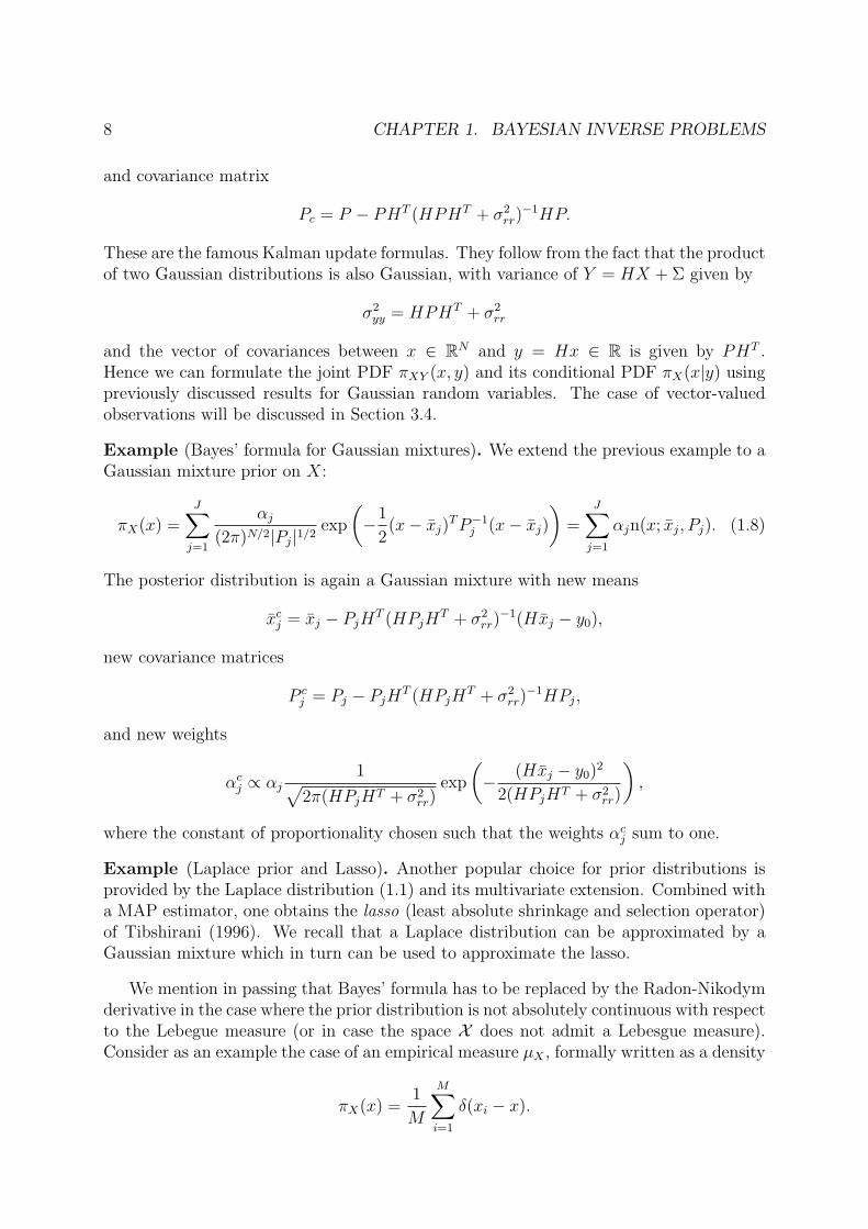
Example (Bayes’ formula for Gaussian mixtures). We extend the previous example to aGaussian mixture prior on X:

πX(x) =J∑

j=1

αj

(2π)N/2|Pj|1/2exp

(−1

2(x− xj)

TP−1j (x− xj)

)=

J∑j=1

αjn(x; xj, Pj). (1.8)

The posterior distribution is again a Gaussian mixture with new means

xcj = xj − PjH

T (HPjHT + σ2

rr)−1(Hxj − y0),

new covariance matrices

P cj = Pj − PjH

T (HPjHT + σ2

rr)−1HPj,

and new weights

αcj ∝ αj

1√2π(HPjHT + σ2

rr)exp

(− (Hxj − y0)

2

2(HPjHT + σ2rr)

),

where the constant of proportionality chosen such that the weights αcj sum to one.

Example (Laplace prior and Lasso). Another popular choice for prior distributions isprovided by the Laplace distribution (1.1) and its multivariate extension. Combined witha MAP estimator, one obtains the lasso (least absolute shrinkage and selection operator)of Tibshirani (1996). We recall that a Laplace distribution can be approximated by aGaussian mixture which in turn can be used to approximate the lasso.

We mention in passing that Bayes’ formula has to be replaced by the Radon-Nikodymderivative in the case where the prior distribution is not absolutely continuous with respectto the Lebegue measure (or in case the space X does not admit a Lebesgue measure).Consider as an example the case of an empirical measure µX , formally written as a density

πX(x) =1

M

M∑i=1

δ(xi − x).

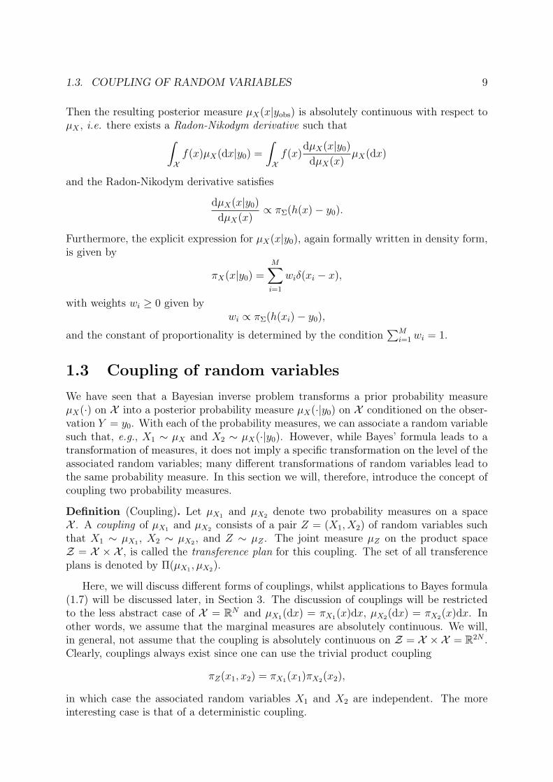
1.3. COUPLING OF RANDOM VARIABLES 9

Then the resulting posterior measure µX(x|yobs) is absolutely continuous with respect toµX , i.e. there exists a Radon-Nikodym derivative such that∫

Xf(x)µX(dx|y0) =

∫Xf(x)

dµX(x|y0)

dµX(x)µX(dx)

and the Radon-Nikodym derivative satisfies

dµX(x|y0)

dµX(x)∝ πΣ(h(x)− y0).

Furthermore, the explicit expression for µX(x|y0), again formally written in density form,is given by

πX(x|y0) =M∑i=1

wiδ(xi − x),

with weights wi ≥ 0 given bywi ∝ πΣ(h(xi)− y0),

and the constant of proportionality is determined by the condition∑M

i=1wi = 1.

1.3 Coupling of random variables

We have seen that a Bayesian inverse problem transforms a prior probability measureµX(·) on X into a posterior probability measure µX(·|y0) on X conditioned on the obser-vation Y = y0. With each of the probability measures, we can associate a random variablesuch that, e.g., X1 ∼ µX and X2 ∼ µX(·|y0). However, while Bayes’ formula leads to atransformation of measures, it does not imply a specific transformation on the level of theassociated random variables; many different transformations of random variables lead tothe same probability measure. In this section we will, therefore, introduce the concept ofcoupling two probability measures.

Definition (Coupling). Let µX1 and µX2 denote two probability measures on a spaceX . A coupling of µX1 and µX2 consists of a pair Z = (X1, X2) of random variables suchthat X1 ∼ µX1 , X2 ∼ µX2 , and Z ∼ µZ . The joint measure µZ on the product spaceZ = X × X , is called the transference plan for this coupling. The set of all transferenceplans is denoted by Π(µX1 , µX2).

Here, we will discuss different forms of couplings, whilst applications to Bayes formula(1.7) will be discussed later, in Section 3. The discussion of couplings will be restrictedto the less abstract case of X = RN and µX1(dx) = πX1(x)dx, µX2(dx) = πX2(x)dx. Inother words, we assume that the marginal measures are absolutely continuous. We will,in general, not assume that the coupling is absolutely continuous on Z = X × X = R2N .Clearly, couplings always exist since one can use the trivial product coupling

πZ(x1, x2) = πX1(x1)πX2(x2),

in which case the associated random variables X1 and X2 are independent. The moreinteresting case is that of a deterministic coupling.


Definition (Deterministic coupling). Assume that we have a random variable X1 withlaw µX1 and a probability measure µX2 . A diffeomorphism T : X → X is called a transportmap if the induced random variable X2 = T (X1) satisfies∫

Xf(x2)µX2(dx2) =

∫Xf(T (x1))µX1(dx1)

for all suitable functions f : X → R. The associated coupling

µZ(dx1, dx2) = δ(x2 − T (x1))µX1(dx1)dx2,

where δ(·) is the standard Dirac distribution, is called a deterministic coupling. Note thatµZ is not absolutely continuous even if both µX1 and µX2 are.

Using ∫Xf(x2)δ(x2 − T (x1))dx2 = f(T (x1)),

it indeed follows from the above definition of µZ that∫Zf(x2)µZ(dx1, dx2) =

∫Zf(T (x1))µZ(dx1, dx2).

We now discuss a simple example.

Example (One-dimensional transport map). Let πX1(x) and πX2(x) denote two PDFson X = R. We define the associated cumulative distribution functions by

FX1(x) =

∫ x

−∞πX1(x

′)dx′, FX2(x) =

∫ x

−∞πX2(x

′)dx′.

Since FX2 is monotonically increasing, it has a unique inverse F−1X2

given by

F−1X2

(p) = infx ∈ R : FX2(x) > p

for p ∈ [0, 1]. The inverse may be used to define a transport map that transforms X1 intoX2 as follows,

X2 = T (X1) = F−1X2

(FX1(X1)).

For example, consider the case where X1 is a random variable with uniform distributionU([0, 1]) and X2 is a random variable with standard uniform distribution N(0, 1). Thenthe transport map between X1 and X2 is simply the inverse of the cumulative distributionfunction

FX2(x) =1√2π

∫ x

−∞e−(x′)2/2dx′,

which provides a standard tool for converting uniformly distributed random numbers innormally distributed ones.

We now extend this transform method to random variables in RN with N = 2.

1.3. COUPLING OF RANDOM VARIABLES 11

Example (Knothe-Rosenblatt rearrangement). Let πX1(x1, x2) and πX2(x

1, x2) denotetwo PDFs on x = (x1, x2) ∈ R2. A transport map between πX1 and πX2 can be constructedin the following manner. We first find the two one-dimensional marginals πX1

1(x1) and

πX12(x1) of the two PDFs. We had seen in the previous example how to construct a

transport map X12 = T1(X

11 ) which couples these two one-dimensional marginal PDFs.

Here X1i denotes the first component of the random variables i = 1, 2. Next we write

πX1(x1, x2) = πX1(x

2|x1)πX11(x1), πX2(x

1, x2) = πX2(x2|x1)πX1

2(x1)

and find a transport map X22 = T2(X

11 , X

21 ) by considering one-dimensional couplings

between πX1(x2|x1) and πX2(x

2|T (x1)) with x1 fixed. The associated joint distribution isgiven by

πZ(x11, x

21, x

12, x

22) = δ(x1

2 − T1(x11))δ(x

22 − T2(x

11, x

21))πX1(x

11, x

21).

This is called the Knothe-Rosenblatt rearrangement, also well-known to statisticiansunder the name of conditional quantile transforms. It can be extended to RN , N ≥ 3 inthe obvious way by introducing the conditional PDFs

πX1(x3|x1, x2), πX2(x

3|x1, x2),

and by constructing an appropriate map X32 = T3(X

11 , X

21 , X

31 ) from those conditional

PDFs for fixed pairs (x11, x

21) and (x1

2, x22) = (T1(x

11), T2(x

11, x

21)) etc. While the Knothe-

Rosenblatt rearrangement can be used in quite general situations, it has the undesirableproperty that the map depends on the choice of ordering of the variables i.e., in twodimensions a different map is obtained if one instead first marginalises out the x1 compo-nent.

Example (Affine transport maps for Gaussian distributions). Consider two Gaussiandistributions N(x1,Σ1) and N(x2,Σ2) in RN with means x1 and x2 and covariance matricesΣ1 and Σ2, respectively. Then the affine transformation

x2 = T (x1) = x2 + Σ1/22 Σ

−1/21 (x1 − x1)

provides a deterministic coupling. Indeed, we find that

(x2 − x2)T Σ−1

2 (x2 − x2) = (x1 − x1)T Σ−1

1 (x1 − x1)

under the suggested coupling. The proposed coupling is, of course, not unique since

x2 = T (x1) = x2 + Σ1/22 QΣ

−1/21 (x1 − x1),

where Q is an orthogonal matrix, also provides a coupling.

Deterministic couplings can be viewed as a special case of Markov couplings

πX2(x2) =

∫X1

π(x2|x1)πX1(x1)dx1,

where π(x2|x1) denotes an appropriate conditional PDF for the random variable X2 givenX1 = x1. Indeed, we simply have

π(x2|x1) = δ(x2 − T (x1))


for deterministic couplings. We will come back to Markov couplings and, more generally,Markov processes in Section 2.

The trivial coupling πZ(x1, x2) = πX1(x1)πX2(x2) leads to a zero correlation betweenthe induced random variables X1 and X2 since

cor(X1, X2) = EZ [(x1 − x1)(x2 − x2)T ] = EZ [x1x

T2 ]− x1x

T2 = 0,

where xi = EXi[x]. A transport map leads instead to the correlation matrix

cor(X1, X2) = EZ [x1xT2 ]− EX1 [x1](EX2 [x2])

T = EX1 [x1T (x1)T ]− x1x

T2 ,

which is non-zero in general. If several transport maps exists then one could choose theone that maximizes the correlation. Consider, for example, univariate random variablesX1 and X2, then maximising their correlation for given marginal PDFs has an importantgeometric interpretation: it is equivalent to minimizing the mean square distance betweenx1 and T (x1) = x2 given by

EZ [|x2 − x1|2] = EX1 [|x1|2] + EX2 [|x2|2]− 2EZ [x1x2]

= EX1 [|x1|2] + EX2 [|x2|2]− 2EZ [(x1 − x1)(x2 − x2)]− 2x1x2

= EX1 [|x1|2] + EX2 [|x2|2]− 2x1x2 − 2cor(X1, X2).

Hence finding a joint measure µZ that minimization the expectation of (x1 − x2)2 simul-

taneously maximizes the correlation between X1 and X2. This geometric interpretationleads to the celebrated Monge-Kantorovitch problem.

Definition (Monge-Kantorovitch problem). A transference plan µ∗Z ∈ Π(µX1 , µX2) iscalled the solution to the Monge-Kantorovitch problem with cost function c(x1, x2) =‖x1 − x2‖2 if

µ∗Z = arg infµZ∈Π(µX1

,µX2)EZ [‖x1 − x2‖2]. (1.9)

The associated function

W (µX1 , µX2) = EZ [‖x1 − x2‖2], law(Z) = µ∗Z

is called the L2-Wasserstein distance of µX1 and µX2 .

Theorem (Optimal transference plan). If the measures µXi, i = 1, 2, are absolutely con-

tinuous, then the optimal transference plan that solves the Monge-Kantorovitch problemcorresponds to a deterministic coupling with transfer map

X2 = T (X1) = ∇xψ(x),

for some potential function ψ : RN → R.

Proof. We only demonstrate that the solution to the Monge-Kantorovitch problem isof the desired form when the infimum in (1.9) is restricted to deterministic couplings.See Villani (2003) for a complete proof and also for more general results in terms ofsubgradients and weaker conditions on the two marginal measures.

1.4. MONTE CARLO METHODS 13

We denote the associated PDFs by πXi, i = 1, 2. We also introduce the inverse transfer

map X1 = S(X2) = T−1(X2) and consider the functional

L[S,Ψ] =1

2

∫RN

‖S(x)− x‖2πX2(x)dx+∫RN

[Ψ(S(x))πX2(x)−Ψ(x)πX1(x)] dx

in S and a potential Ψ : RN → R. We note that∫RN

[Ψ(S(x))πX2(x)−Ψ(x)πX1(x)] dx =∫RN

Ψ(x) [πX2(T (x))|DT (x)| − πX1(x)] dx

by a simple change of variables. Here |DT (x)| denotes the determinant of the Jacobianmatrix of T at x and the potential Ψ can be interpreted as a Lagrange multiplier enforcingthe coupling of the two marginal PDFs under the desired transport map.

Taking variational derivatives with respect to S and Ψ, we obtain two equations

δLδS

= πX2(x) ((S(x)− x) +∇xΨ(S(x))) = 0

andδLδΨ

= −πX1(x) + πX2(T (x))|DT (x)| = 0 (1.10)

characterizing critical points of the functional L. The first equality implies

x2 = x1 +∇xΨ(x1) = ∇x

(1

2xT

1 x1 + Ψ(x1)

)= ∇xψ(x1)

and the second implies that T transforms πX1 into πX2 .

While optimal couplings are of broad theoretical and practical interest, their compu-tational implementation can be very demanding. In Section 3, we will discuss an em-bedding method originally due to Moser (1965), which leads to a generally non-optimalbut computationally tractable formulation in the context of Bayesian statistics and dataassimilation.

1.4 Monte Carlo methods

Monte Carlo methods, also called particle or ensemble methods depending on the contextin which they are being used, can be used to approximate statistics, namely expectationvalues EX [f ], for a random variable X. We begin by discussing the special case f(x) = x,namely, the mean.


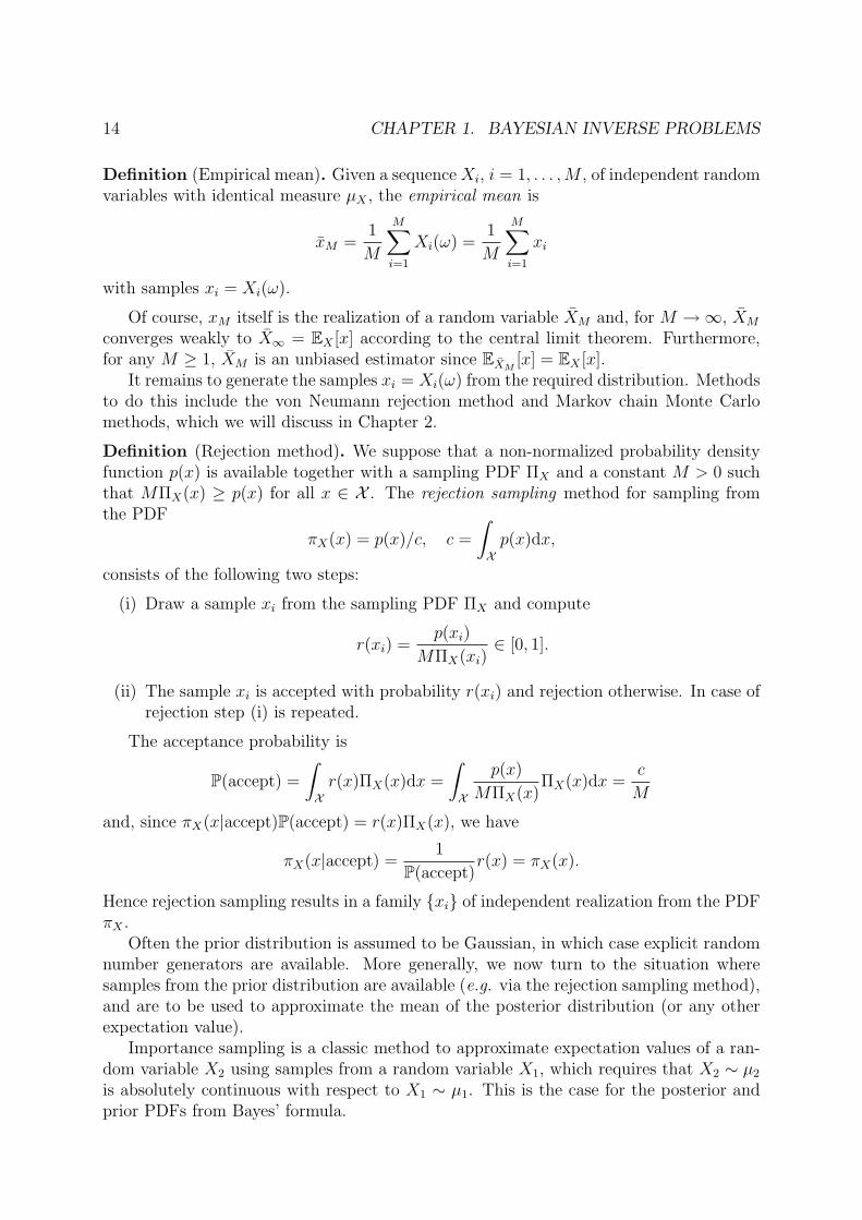
Definition (Empirical mean). Given a sequenceXi, i = 1, . . . ,M , of independent randomvariables with identical measure µX , the empirical mean is

xM =1

M

M∑i=1

Xi(ω) =1

M

M∑i=1

xi

with samples xi = Xi(ω).

Of course, xM itself is the realization of a random variable XM and, for M →∞, XM

converges weakly to X∞ = EX [x] according to the central limit theorem. Furthermore,for any M ≥ 1, XM is an unbiased estimator since EXM

[x] = EX [x].It remains to generate the samples xi = Xi(ω) from the required distribution. Methods

to do this include the von Neumann rejection method and Markov chain Monte Carlomethods, which we will discuss in Chapter 2.

Definition (Rejection method). We suppose that a non-normalized probability densityfunction p(x) is available together with a sampling PDF ΠX and a constant M > 0 suchthat MΠX(x) ≥ p(x) for all x ∈ X . The rejection sampling method for sampling fromthe PDF

πX(x) = p(x)/c, c =

∫Xp(x)dx,

consists of the following two steps:

(i) Draw a sample xi from the sampling PDF ΠX and compute

r(xi) =p(xi)

MΠX(xi)∈ [0, 1].

(ii) The sample xi is accepted with probability r(xi) and rejection otherwise. In case ofrejection step (i) is repeated.

The acceptance probability is

P(accept) =

∫Xr(x)ΠX(x)dx =

∫X

p(x)

MΠX(x)ΠX(x)dx =

c

M

and, since πX(x|accept)P(accept) = r(x)ΠX(x), we have

πX(x|accept) =1

P(accept)r(x) = πX(x).

Hence rejection sampling results in a family xi of independent realization from the PDFπX .

Often the prior distribution is assumed to be Gaussian, in which case explicit randomnumber generators are available. More generally, we now turn to the situation wheresamples from the prior distribution are available (e.g. via the rejection sampling method),and are to be used to approximate the mean of the posterior distribution (or any otherexpectation value).

Importance sampling is a classic method to approximate expectation values of a ran-dom variable X2 using samples from a random variable X1, which requires that X2 ∼ µ2

is absolutely continuous with respect to X1 ∼ µ1. This is the case for the posterior andprior PDFs from Bayes’ formula.

1.4. MONTE CARLO METHODS 15

Definition (Importance sampling). Let xpriori , i = 1, . . . ,M , denote samples from the

prior PDF πX , then the important sampler estimate of the mean of the posterior is

xpostM =

M∑i=1

wixpriori (1.11)

with importance weights

wi =πY (y0|xprior

i )∑Mi=1 πY (y0|xprior

i ). (1.12)

Another point of view is that statistics obtained in this way are exact statistics forthe weighted empirical measure

πemX (x) =

M∑i=1

wiδ(x− xpriori ).

Importance sampling becomes statistically inefficient when the weights have largelyvarying magnitude, which becomes particularly significant for high-dimensional problems.To demonstrate this effect consider a uniform prior on the unit hypercube V = [0, 1]N .Each of the M samples xi from this prior formally represent a hypercube with volume1/M . However, the likelihood measures the distance of a sample xi to the observation y0

in the Euclidean distance and the volume of a hypersphere decreases rapdily relative tothat of an associated hypercube as N increases.

To counteract this curse of dimensionality, one may utilize the concept of coupling. SeeFig. 1.1. In other words, assume that we have a transport map x2 = T (x1) which couplesthe prior and posterior distributions. Then, with transformed samples xpost

i = T (xpriori ),

we obtain the estimator

xpostM =

M∑i=1

wixposti (1.13)

with optimal weights wi = 1/M .Sometimes one cannot couple the prior and posterior distribution directly, or the

coupling is too expensive computationally. Then one can attempt to find a cou-pling between the prior PDF πX and an approximation π′X(x|y0) to the posterior PDFπX(x|y0) ∝ πY (y0|x)πX(x). Given an associated transport map x2 = T ′(x1), one obtains

xpostM =

M∑i=1

wix′i (1.14)

with x′i = T ′(xi) and weights

wi ∝πY (y0|x′i)πX(x′i)

π′X(x′i|y0), (1.15)

i = 1, . . . ,M , with the contstant of proportionality chosen such that∑M

i=1 wi = 1. Indeedif π′X(x|y0) = πX(x|y0) we are back to equal weights wi = 1/M and π′X(x|y0) = πX(x)leads back to the classic importance sampling using the prior samples, i.e. x′i = xi.


PDFs

RVs

MC

Figure 1.1: A cartoon like picture of the relation between Bayes formula at the level ofPDFs, associated coupled random variables and Monte Carlo sampling methods.

A weighted empirical measure of the form given in (1.13) can also be approximatedby another empirical measure with equal weights by resampling. The idea is to replaceeach of the original samples xi by ξi ≥ 0 offsprings with equal weights wi = 1/M . Thedistribution of offsprings is chosen to be equal to the distribution of M samples (withreplacement) drawn at random from the empirical distribution (1.13). In other words,the offsprings ξiM

i=1 follow a multinomial distribution defined by

P(ξi = ni, i = 1, . . . ,M) =M !∏Mi=1 ni!

M∏i=1

(wi)ni (1.16)

with ni ≥ 0 such that∑

i ni = M . Independent resampling is often replaced by residualresampling.

Definition (Residual resampling). Residual resampling generates

ξi = bMwic+ ξi,

offsprings of each ensemble member xi with weight wi, i = 1, . . . ,M . Here bxc denotesthe integer part of x and ξi follows the multinomial distribution (1.16) with M beingreplaced by

M = M −∑

i

bMwic

1.5. ESTIMATING DISTRIBUTIONS FROM SAMPLES 17

and weights wi being replaced by

wi =Mwi − bMwic∑M

j=1(Mwj − bMwjc).

1.5 Estimating distributions from samples

In same cases, the explicit form of the prior distribution πX is not known and can only beinferred from available realizations xi = X(ωi), law(X) = πX . This is a classic problem instatistics and one distinguishes between parametric and non-parametric statistics. Herewe will discuss two methods for parametric statistics, where one assumes knowledge aboutthe principal structure of πX such as being Gaussian.

Let us assume that we got M independen realizations xi ∈ RN of a Gaussian randomvariable with unknown mean x and unknown covariance matrix Σ. How can be find areliable estimator for those unknown quantities given our M realizations? We had alreadyintroduced the estimator

xM =1

M

∑i

xi

for the mean. An estimator for the covariance matrix is provided

Pm =1

M − 1

∑i

(xi − x)(xi − x)T . (1.17)

Furthermore, assuming that N = 1 for a moment and that the xi’s are treated as i.i.d.random variables with mean x and covariance σ2, we would find that the central limittheorem implies that the random variable (xM − x)

√M/σ behaves like a Gaussian ran-

dom variable with mean zero and variance equal to one for M → ∞ in the sense of itsdistribution. Furthermore, for any finite M we have

E[xM ] =1

M

M∑i=1

x = x

and the estimator is called unbiased. Similar statements can be derived for the empiricalcoveriance estimator.

Let us take another route of deriving empirical estimators for the mean and the co-variance matric. For that we write

1

(2π)N/2|Σ|1/2exp

(−1

2(x− x)T Σ−1(x− x)

)= exp(−L(x; θ)),

where the log-likelihood function L is defined as

L(x; θ) = −1

2log |Σ| − 1

2(x− x)T Σ−1(x− x)− N

2log 2π

and the unknown mean and covariance matrix are collected formally into a vector θ. Ina maximum likelihood approach one now solves the following maximization problem

θ∗ = arg maxθ

1

M

M∑i=1

L(xi, θ)


and θ∗ is taken as the empirical estimate for the mean and the covariance matrix. Notethat

1

M

∑i

L(xi, θ) = Eπem [L(x, θ)]

with empirical measure

πem(x) =1

M

∑i

δ(x− xi).

To obtain explicit formulas, we need to find the gradient ∇θL(x; θ). We now revertback to gradients with respect to x and Σ, respectively. The gradient with respect to xis simply given by

∇xL(x; θ) = Σ−1(x− x)

and we obtain for the associated estimator

M∑i=1

Σ−1(xi − x) = 0

which, provided Σ−1 exists is equivalent to the standard empirical estimate for the mean.To get a sense of where to go let us start with N = 1 and Σ = s > 0. Then simple

calculations reveal

d

ds

(−1

2log s− (x− x)2/2s

)=

1

2s+ (x− x)2/2s2)

and the estimate becomesM∑i=1

(s+ (xi − x)2

)= 0

and

s =1

M

M∑i=1

(xi − x)2,

which is almost identical to the previously stated estimator for the variance. The dif-ference stems from the fact that the maximum likelihood estimator is biased for finiteM . However, this is only of signficance for relatively small number of realizations M .Nevertheless, (1.17) should be used in practice.

Finding the gradient of L with respect to the covariance matrix Σ is quite a bit tougher.First we define the gradient of a functional f(Σ) ∈ RN×N using the directional derivative.This yields

〈∇Σf(Σ), D〉 = trace((∇Σf(Σ))TD) = limε→0

f(Σ + εD)− f(Σ)

ε

for all D ∈ RN×N . The first equality is simply the definition of the inner product

〈A,B〉 = trace(ATB)


for the space of matrices A,B ∈ RN×N (inducing the Frobenius matrix norm). Next wenote that

uT Σ−1v = trace(uvT Σ−1) = trace(Σ−1vuT ),

which implies

limε→0

uT (Σ + εD)−1v − uT Σ−1v

ε= −trace(uvT Σ−2D) = −〈Σ−2vuT , D〉.

Hence we obtain

∇Σ(x− x)T Σ−1(x− x) = −Σ−2(x− x)(x− x)T

Next we need to find ∇Σ log |Σ|. Here we make use that Σ is symmetric and positivesemi-definite and diagonalize Σ, i.e. Σ = QΛQT , where Q is orthogonal and Λ is diagonalwith diagonal entries λj ≥ 0. Then log |Σ| =

∑Nj=1 log λj,

log |Λ + εD| = log

(K∑

j=1

(λi + εdii)∏i6=j

λj

)+O(ε2).

and

limε→0

log |Λ + εD| − log |Λ|ε

= trace(Λ−1D) = 〈Σ−1, D〉

Therefore ∇Σ log |Σ| = Σ−1. In summary, we obtain

∇ΣL(x; θ) = −1

2Σ−1 +

1

2Σ−2(x− x)(x− x)T

and the maximum likelihood estimate of Σ follows from

0 =M∑i=1

∇ΣL(xi, θ) = −mΣ−1 +M∑i=1

Σ−2(xi − x)(xi − x)T

after left multiplication by Σ2 and division by M .We will now consider the following more general situation. Let samples xi, i =

1, . . . ,m, of a random variable X be given. Let us assume that we also know that thegenerating distribution is a mixture of K Gaussians with unknown mean xk and unknowncovariance matrix Pk. We also do not know the relative weight αk ≥ 0 of each Gaussian.Hence we can only make the ansatz

πX(x) =K∑

k=1

αkn(x; xk, Pk) (1.18)

with unknown weights αk ≥ 0,∑

k αk = 1, mean xk, and covariance matrix Pk, k =1, . . . , K.

In principle, one could treat this problem by the maximum likelihood method as muchas we did this before in case of a single Gaussian, i.e. K = 1. But let us pause for amoment and have a closer look at the problem. We notice that there is a hidden piece of


information, namely which Gaussian component a particular realization xi has been drawnfrom. Let us denote this unknown/hidden random variable by Y ∈ Y = 1, . . . , K. Sincewe treat Y as a random variable its distribution should be πY = (α1, . . . , αK)T ∈ RK inagreement with the ansatz (1.18).

Finding the parameters of (1.18) would be easy if we were provided the hidden variableY for each sample xi, i.e., if were given pairs (xi, yi) ∈ Rn × Y . Then a maximumlikelihood approach would determine αk by the relative frequency of k in the realizationsyi, i = . . . ,m, and the mean xk and covariance matrice Pk would be estimated in thestandard manner using all realizations xi for which yi = k. The bad news is that oftenwe do not have any direct access to Y .

However, one can utilize the following strategy. Let us assume that we have found orguessed an initial parameter set θ0 = α0

k, x0k, P

0k K

k=1. Then we can assign a probabilityp0

ki to each sample xi which represents the conditional probability that xi has been drawnfrom the kth Gaussian. Using (1.18), the explicit expression

p0ki = πY (y = k|xi, θ

0) =α0

kn(xi; x0k, P

0k )∑K

l=1 α0l n(xi; x0

l , P0l )

is found.With this newly gained additional piece of information we can now return to the

problem of actually estimating θ using a maximum likelihood approach. We find from(1.18) and the previous discussion on fitting a single Gaussian that the log-likelihood ofθ given that x was drawn from the kth Gaussian is

L(θ;x, y = k) = logαk −1

2log |Pk| −

1

2(x− xk)(Pk)

−1(x− xk)−N

2log 2π

We now take the expectation of L(θ;x, y) with respect to the joint conditional densityπXY (x, y|θ0) as approximated by the empirical measure

πemXY (x, y|θ) =

1

m

∑m

∑k

δ(x− xi)p0kiδk,y

where δky denotes the Kronecker delta, i.e. δky = 1 if y = k and δky = 0 otherwise. As inthe standard maximum likelihood approach we now define

θ∗ = arg maxθQ(θ, θ0)

withQ(θ, θ0) = Eπem

XY[L(θ;x, y)]

The maximization can be carried out explicitly and we obtain a new set of parametersθ1 = θ∗ given by

α1k =

1

M

M∑i=1

p0ki,

as well as

x1k =

∑i p

0kixk∑

j p0kj


and

P 1k =

1∑j p

0kj

M∑i=1

p0ki(xi − x1

k)(xi − x1k)

T .

This process can be repeated with θ0 being replaced by θ1 and is continued till convergence.What we have just witnessed is a special instance of the expectation-maximization

(EM) algorithm. The basis construction principle is a set of realization xi of a randomvariable x with which we associate the emprical measure

πemX (x) =

1

M

M∑i=1

δ(xi − x).

There is also a hidden random variable which we cannot access directly. We assume thatthe hidden variable is a finite random variable Y ∈ Y = 1, 2, . . . , K and that the desiredmarginalized PDF is

πX(x|θ) =K∑

k=1

πXY (x, y = k|θ)

with πXY (x, y|θ) being specified apriori.Given a current set of parameters θs, s ≥ 0, the associated joint density in (x, y)

conditioned on θs is used to estimate the conditional probability pski that sample xi belongs

to the kth mixture component, i.e.

pski = πY (y = k|x = xi, θ

s) =πXY (xi, y = k|θs)∑l πXY (xi, y = l|θs)

.

This in turn allows us to state an empirical measure approximation for the joint distribu-tion in (x, y) of the form

πemXY (x, y|θs) =

1

m

M∑i=1

K∑k=1

δ(x− xi)pski. (1.19)

The next step is to compute the expectation

Q(θ, θs) = EπemXY

[log π(x, y|θ)]

=1

M

M∑i=1

K∑k=1

pski log π(xi, k|θs)

with respect to the empirical measure (1.19). The function Q(θ, θs) is finally maximizedto yield a new set of parameters θs+1 via

θs+1 = arg maxθQ(θ, θs).

The process is interated till convergence.The EM algorithm only converges locally and may fail due to inappropriate starting

values and inappropriate number of mixture components. To make the EM algorithm


more robust It has been proposed to instead maximize a posterior based on combiningthe likelihood function with an appropriate prior density for the unknown parametersof the statistical model. The approach is closely related to the regularization approachdiscussed in Appendix A for the single Gaussian case and can be viewed as regularizingan ill-posed inverse problem.

So far we have investigated cases of parametric statistics. We now discuss kerneldensity estimation as an example of non-parametric statistics.

Definition (Univariate kernel density estimation). Let xi ∈ R, i = 1, . . . ,M , be in-dependent samples from an unknown density πX . The kernel density estimator of πX

is

πX,h(x) =1

hM

M∑i=1

K

(x− xi

h

)for a suitable kernel function K(x) ≥ 0 with

∫RK(x)dx = 1. We will work with the

Gaussian kernel

K(x) =1√2πe−x2/2.

The parameter h > 0 is called the bandwidth.

Kernel density estimators can be viewed as smoothed empirical measures. The amountof smoothing is controlled by the bandwidth parameter h. Hence selection of the band-width is of crucial importance for the performance of a kernel density estimator. Manybandwidth selectors are based on the mean integrated squared error defined by

MISE(h) =

∫R

(BIAS(x, h)2 + VAR(x, h)

)dx

with bias

BIAS(x, h) =M∑i=1

∫R

1

hMK

(x− xi

h

)πX(xi)dxi − πX(x)

=1

h

∫RK

(x− x′

h

)πX(x′)dx′ − πX(x)

and variance

VAR(x, h) =

∫RM

1

hM

M∑i=1

K

(x− xi

h

)2

πX(x1) · · ·πX(xM)dx1 · · · dxM−

1

h2

(∫RK

(x− x′

h

)πX(x′)dx′

)2

=M∑i=1

∫R

1

hMK

(x− xi

h

)2

πX(xi)dxi−

1

h2M

(∫RK

(x− x′

h

)πX(x′)dx′

)2

=1

h2M

∫RK

(x− x′

h

)2

πX(x′)dx′ − 1

h2M

(∫RK

(x− x′

h

)πX(x′)dx′

)2

.


We note that the bias vanished for h → 0 while the variances increases unless we alsoincrease the sample size M appropriately.

The MISE is based on taking the expectation of (πX,h(x) − πX(x)) over all possibleindependent samples xi following the law πX . Let us write this expectation as

E[(πX,h(x)− πX(x))2] = E[(πX,h(x)− E[πX,h(x)])2] + (E[πX,h(x)]− πX(x))2.

The first term on the left hand side yields VAR(x, h) while the second term givesBIAS(x, h).

We now derive an asymptotic approximation formula. Recall the Taylor expansion

πX(x+ hz) = πX(x) + hπ′X(x)z +h2

2π′′X(x)z2 +O(h3),

set hz = x′−x and make use of the fact that typical kernel functions satisfyK(x) = K(−x)to obtain, for example,

BIAS(x, h) =h2π′′X(x)

2

∫Rz2K(z)dz +O(h3)

and, after some more calculations,

MISE(h) ≈∫

R

h4

(π′′X(x)

2k2

)2

+1

MhπX(x)

∫RK(z)2dz

dx,

where k2 =∫

R z2K(z)dz.

Minimization with respect to h yields

hopt =

∫RK(z)2dz

Mk2

∫R(π′′X(x))2dx

1/5

.

Explicit calculation of hopt requires knowledge of πX which, however, is not known. Asimple estimate for hopt can be obtained by assuming that πX is Gaussian with varianceσ2. Then ∫

Rπ′′X(x)dx =

3

8√πσ−5 ≈ 0.212σ−5,

which leads to Silverman’s rule of thumb

hopt ≈ 1.06σM−1/5.

Here the variance σ2 is to be estimated from the data set.A different approach is to write

MISE(h) =

∫RπX(x)2dx− 2

∫R

E[πX(x)πX,h(x)]dx+

∫R

E[πX,h(x)2]dx

and to estimate the h dependent terms by leave-one-out cross validation. This approachyields the unbiased estimator

LSCV(h) =

∫RπX,h(x)

2dx− 2

M

M∑i=1

π(i)X,h(xi)

=

∫RπX,h(x)

2dx− 2

M − 1

M∑i=1

(πX,h(xi)−

K(0)

hM

).


Here π(i)X,h(x) is the leave-one-out kernel density estimator

π(i)X,h(x) =

1

M − 1

∑k,k 6=i

1

hK

(x− xk

h

).

Again, a suitable bandwidth can be obtained by minimizing LSCV(h).

References

An excellent introduction to many topics covered in this survey is Jazwinski (1970).Bayesian inference and a Bayesian perspective on inverse problems are discussed in Kaipioand Somersalo (2005), Neal (1996), Lewis et al. (2006). The two monographs by Villani(2003, 2009) provide an in depth introduction to optimal transportation and coupling ofrandom variables. Monte Carlo methods are covered in Liu (2001). See also Bain andCrisan (2009) for resampling methods with minimal variance. A discussion of infinite-dimensional Bayesian inverse problems can be found in Stuart (2010). Kernel densityestimators are discussed, for example, in Wand and Jones (1995). A broad perspectiveon statistical learning techniques is provided by Hastie et al. (2009).

Appendix A: Regularized estimators for the mean and

the covariance

In many practical applications the number of samples M will be relatively small comparedto the dimension of phase space X = RN and the problem of finding x and Σ is potentiallyill-posed in the sense of inverse problems. In those cases one can can resort to the followingregularization to estimate the mean and the covariance matrix robustly. The essential ideais to imposing appropriate priors on the unknown mean and covariance matrix. Of course,this is nothing else than regularizing an ill-posed inverse problem as discussed beforewithin a Bayesian framework. We first demonstrate the basic idea for one-dimensionaldata. The following prior for the mean

π(x|σ2, κ, µ) ∝(σ2)1/2

exp(− κ

2σ2(x− µ)

)and the variance

π(σ2|ν, ξ) ∝(σ2)− ν+2

2 exp

(− ξ2

2σ2

)have been proposed, where (µ, κ, ν, ξ) are hyperparameters called the mean, shrinkage,degrees of freedom, and scale, respectively. Maximization of the resulting posterior dis-tribution

π(x, σ2|D) ∝m∏

i=1

n(xi; x, σ2)π(x|σ2, κ, µ)π(σ2|ν, ξ)

leads to the (regularized) estimate

xr =Mxs + κµ

κ+M


for the mean and to the (regularized) estimate for the variance

σ2r =

ξ2 + κMκ+M

(xs − µ) +Mσ2s

ν +M + 3,

respectively. Here

xs =1

M

M∑i=1

xi

and

σ2s =

1

M

M∑i=1

(xi − xs)2

denote the standard (non-regularized) maximum likelihood estimates.This regularization approach can be generalized to N -dimensional data xi ∈ RN ,

i = 1, . . . ,M , in which case one uses a normal prior

x ∼ N(µ,Σ/κ)

on the mean and an inverse Wishart prior

Σ ∼ |Σ|−ν+N+1

2 exp

(−1

2trace

[Σ−1Λ−1

])for the covariance matrix. The resulting estimates are given by

xr =Mxs + κµ

κ+M

and

Σr =1

ν +M +N + 2

(Λ−1 +

κM

κ+M(xs − µ)(xs − µ)T +MΣs

),

respectively, with the standard estimates

xs =1

M

M∑i=1

xi

and

Σs =1

M

M∑i=1

(xi − xs)(xi − xs)T ,

respectively. In many application, only the covariance estimate needs to be regularizedin which case one can set µ = xs which implies xr = xs and

Σr =1

ν +M +N + 2

(Λ−1 +MΣs

).

The parameter ν needs to satisfy ν ≥ N + 2 to obtain a finite variance in the prior andone often sets ν to its smalest possible value.


Appendix B: Bayesian model selection

Suppose we want to use some data y0 to compare two competing statistical models M1

and M2 with parameter values θ1 and θ2. As an example, imagine the situation that wefit Gaussian mixture models with different number of mixtures to a set of samples xi,i = 1, . . . ,M from a random variable X. In this case y0 = xi and we also need someconditional PDF of how to assess the likelihood of y0 under model Mi and parametervalues θi. We denote this conditional PDF by πY (y|Mi, θi). Next we define the integratedlikelihood by

πY (y|Mi) =

∫RKi

πY (y|Mi, θi)πΘi(θi|Mi)dθi (1.20)

for i = 1, 2. Then, by Bayes’ formula, the posterior probability that M1 is the correctmodel given the data y0 is

P(M1|y0) =πY (y0|M1)P(M1)

πy(y0|M1)P(M1 + πy(y0|M2)P(M2

with a similar expression for P(M2|y0). A more meaningful quantity is provided by theposterior odds for M2 against M1, defined by

P(M2|y0)

P(M1|y0)=πy(y0|M2)

πy(y0|M1)

P(M2

P(M1

,

which measures the extend to which the data supports M2 over M1.The key factor underlying Bayesian model selection is the integrated likelihood (1.20).

The BIC (Bayesian information criterion) provides a computable approximation to theintegral

πy(y0) =

∫RK

πY (y0|θ)πTheta(θ)dθ

using Laplace method for integrals. We assume that the data y0 consists ofM independentobservations which allows us to expand

g(θ) = log[πY (y0|θ)πTheta(θ)]

abouts is posterior mode θ. Using the quadratic approximation

g(θ) ≈ g(θ) + (θ − θ)Tg′′(θ)(θ − θ)

in the integral one obtains the approximation

πY (y0) ≈ exp(g(θ))(2π)K/2|g′′(θ)|−1/2

with the approximation error being of order O(M−1).Furthermore removing also all terms of order O(M0) leads to the widely used BIC

approximationlog πY (y0) ≈ log πY (y0|θ)− (K/2) logM (1.21)

The fact that (1.21) ignores terms of order O(M0) implies that the estimator does notformally converge even for samples sizes M →∞. Empirical evidence suggests that (1.21)provides nevertheless a useful approximation for computing Bayesian model factors.


Appendix C: Frequentist approach and confidence in-

tervals

Let us consider the problem of estimating the mean m of a Gaussian random variable X ∼N(m,σ2) from M samples xi and known standard deviation σ. In a Bayesian approachto this problem one would consider m as a random variable, place some prior distributionπm on m and apply Bayes’ formula to obtain a posterior distribution conditioned on theobserved samples.

In contrast to the Bayesian approach of estimating m, the frequentist approach treatsthe unknown m as a fixed quantity. It is also assumed that the experiment of drawingM independent samples from X ∼ N(m,σ2) can be repeated arbitrarily often and eachsample gives rise to an estimated mean

x =1

M

M∑i=1

xi

It is easy to verify that x itself is the realization of a random variable X with mean mand standard deviation σ/

√M , i.e X ∼ N(m,σ2/M).

A key notion of the frequentist analysis is the confidence interval.

Definition (Confidence interval). Let 1 − α denote a real in the interval [0, 1] and Y agiven random variable with PDF πY . The 1−α confidence interval of the mean µ = EY [y]is the interval (a, b) such that

P(a < µ < b) =

∫ µ+b

µ−a

πY (y − µ)dy ≥ 1− α

We now set

Y =X −m

σ/M

in the definition of the confidence interval and find that πY (y) = n(y, 0, 1), i.e. µ = 0 andthe standard deviation has been normalized to one. The frequentist’s interpretation of aconfidence interval is now to say that a fraction of 1 − α of all specifically computed x(i.e. realizations of X computed from samples xi, i = 1, . . . ,M) will fall into the interval(m− a,m+ b), where

|m− a| = |m+ b| = σ√Mc,

∫ c

0

1√2πex2/2dx =

1− α

2.

The more common problem of estimating the mean of a Gaussian random variablealso requires estimating the standard deviation σ from samples xi, i = 1, . . . ,M , via

s =

√∑Mi=1(xi − x)2

M − 1.

Again s can be viewed as the realization of a random variable S and we consider theinduced random variable

Y =X −m

S/√M


in the definition of the confidence interval. It can be shown that Y follows the t-distribution of order M − 1 with mean zero and scale parameter one.

Definition (t-distribution of order M). A random variable Y if t-distributed of order Mwith mean m and precision λ if its PDF satisfies

πY (y) = cM

(1 +

λ(y −m)2

M

)−M+12

with the constant cM chosen such that∫

R πY (y)dy = 1. The t-distribution has mean mand finite variance

var(Y ) =1

λ

M

M − 2

for M > 2.

Chapter 2

Stochastic processes

In this section, we collect basic results concerning stochastic processes.

2.1 Preliminaries

Definition (Stochastic process). Let T be a set of indices. A stochastic process is a familyXtt∈T of random variables on a common space X , i.e. Xt(ω) ∈ X .

In the context of dynamical systems, the variable t corresponds to time. We distinguishbetween continuous time t ∈ [0, tend] ⊂ R or discrete time tn = n∆t, n ∈ 0, 1, 2, . . . = T ,with ∆t > 0 a time-increment. In cases where subscript indices can be confusing we willalso use the notations X(t) and X(tn), respectively.

A stochastic process can be seen as a function of two arguments: t and ω. For fixed ω,Xt(ω) becomes a function of t ∈ T , which we call a realization or trajectory of the stochas-tic process. We will restrict to the case where Xt(ω) is continuous in t (with probability1) in the case of a continuous time. Alternatively, one can fix the time t ∈ T and considerthe random variable Xt(·) and its distribution. More generally, one can consider l-tuples(t1, t2, . . . , tl) and associated l-tuples of random variables (Xt1(·), Xt2(·), . . . , Xtl(·)) andtheir joint distributions. This leads to concepts such as temporal correlation.

2.2 Discrete time Markov processes

First, we develop the concept of Markov processes for discrete time processes and startwith a simple example.

Example (Discrete time random walk). We consider a discrete time process with T =0, 1, 2, . . ., i.e. with time increments ∆t = 1, and with the sequence of univariate randomvariables being generated by the recursion

Xn+1 = Xn + Ξn

for i = 0, 1, 2 . . .. Here Ξn ∼ N(0, 1) are independent with respect to each other and allthe Xn’s. To complete the description of the random process we also need to prescribea measure for X0, which we set equal to the Dirac delta centered at x = 0. In other

29

30 CHAPTER 2. STOCHASTIC PROCESSES

words, the random variable X0 takes the value X(ω) = 0 with probability one. From thiswe may simply conclude that X1 is distributed according to N(0, 1) since we know thatΞ0 ∼ N(0, 1) and X0 = 0 almost surely. The next step is more difficult. First we concludethat, given a particular realization x1 = X1(ω), the conditional outcome for X2 must be

X2|x1 = X1(ω) ∼ N(x1, 1).

and, consequently, the joint probability density for (X1, X2) is given by

πX1X2(x1, x2) =1

2πe−

12(x2−x1)2e−

12x21 .

Finally we obtain the marginal distribution for X2 by integration over x = x1:

πX2(x′) =

1

2π

∫Re−

12(x′−x)2e−

12x2

dx.

By induction, we conclude that the recursion

πXn+1(x′) =

∫R

1√2πe

12(x′−x)2πXn(x)dx

covers the general case n ≥ 1. We see that the conditional PDF

πXn+1(x′|x) =

1√2πe−

12(x′−x)2

plays the role of a transition probability density. Since this PDF does not depend on time,we will use the simpler notation π(x′|x).

The example can be generalized in two ways. First, we may allow for multivariaterandom variables and second we can pick more complex transition probably densities.This leads us to the following definition.

Definition (Discrete time Markov processes). The discrete time stochastic processXnn∈T with X = RN and T = 0, 1, 2, . . .) is called a (time-independent) Markovprocess if its joint PDFs can be written as

πn(x0, x1, . . . , xn) = π(xn|xn−1)π(xn−1|xn−2) · · ·π(x1|x0)π0(x0)

for all n ∈ 0, 1, 2, . . . = T . The associated marginal distributions πn = πXn satisfy theChapman-Kolmogorov equation

πn+1(x′) =

∫RN

π(x′|x)πn(x)dx (2.1)

and the process can be recursively repeated to yield a family of marginal distributionsπnn∈T for given π0. This family can also be characterized by the linear Frobenius-Perronoperator

πn+1 = Pπn, (2.2)

which is induced by (2.1).

2.2. DISCRETE TIME MARKOV PROCESSES 31

The above definition is equivalent to the more traditional definition that a process isMarkov if the conditional distributions satisfy

πn(xn|x0, x1, . . . , xn−1) = π(xn|xn−1).

Note that, contrary to Bayes’ formula (1.7), which directly yields marginal distribu-tions, the Chapman-Kolmogorov equation (2.1) starts from a given coupling

πXn+1Xn(xn+1, xn) = π(xn+1|xn)πXn(xn)

followed by marginalization to derive πXn+1(xn+1). A Markov process is called time-dependent if the conditional PDF π(x′|x) depends on tn. While we have considered time-independent processes in this section, we will see in Section 3 that the idea of couplingapplied to Bayes’ formula leads to time-dependent Markov processes.

Example (Markov processes from dynamical systems). Let us given a map T : X → X .This maps gives rise to a dynamical system via the recursion

xn+1 = T (xn), n ≥ 0.

Typically one would consider trajectories xnn≥0 for given initial condition x0 ∈ X . Ifwe view the initial condition as the realization of a random variable X0 ∼ π0, then thedynamical system gives rise to a Markov process with transition probability

π(x′|x) = δ(x′ − T (x))

We have encountered such transition probabilities already in the context of transportmaps and recall that

πn+1(T (x))|DT (x)| = πn(x)

is the transformation formula for the associated marginal PDFs if T is a diffeomorphism.See Appendix A for more details on dynamical systems.

We now discuss some more specific examples.

Example (Logistic map). We now discuss a non-invertible map T . The logistic mapΨ : [0, 1] → [0, 1] is defined by

xn+1 = axn(1− xn)

wit 0 < a ≤ 4 being a parameter. Here the state space is given by X = [0, 1]. We computetwo time-series starting from x0 = 0.1 and parameter values a = 3.83 and a = 3.99027.Next we start from a uniform distribution and demonstrate its asymptotic evolution underthe logistic map, ToDo: limit set for the support of the evolving PDF, Cantor set

Example (Linear systems). We discuss general linear Markov models

Xn+1 = MXn + c+ Ξn,

X = RN , Ξn ∼ N(0, Q), M ∈ RN×N invertible, c ∈ RN . ToDo: Discuss first Q = 0.Introduce concept of stationary solution, stability of stationary solution, convergence ofinitial PDF to Dirac delta centered about the stationary point. Then discuss general caseQ 6= 0.


We complete this section by a discussion of the linear Frobenius-Perron operator (2.2)in the context of finite state space models.

Example (Discrete state space Markov process). Often random variables are definedover a finite state space X such as X = 1, 2, . . . , S. In this case, each random variableXn : Ω → X is entirely characterized by an S-tuple of non-negative numbers pn(i) =P(Xn = i), i = 1, . . . , S, which also satisfy

∑i pn(i) = 1. A discrete-time Markov process

is now defined through transition probabilities pji = P(Xn+1 = j|Xn = i) which we collectin a S × S transition matrix P . This transition matrix replaces the Frobenius-Perronoperator in (2.2) and we obtain instead the linear recursion

pn+1(j) =S∑

i=1

pjipn(i)

for the state probabilities pn+1(j). A matrix P with entries pji = (P )ji such that (i)pij ≥ 0 and (ii)

∑j pji = 1 is also called a stochastic matrix.

2.3 Stochastic difference and differential equations

We start from the stochastic difference equation

Xn+1 = Xn + ∆f(Xn) +√

2∆tZn, tn+1 = tn + ∆t, (2.3)

where ∆t > 0 is a small parameter (the step-size), f : RN → RN is a given (Lipschitz con-tinuous) function, and Zn ∼ N(0, Q) are independent and identically distributed randomvariables with correlation matrix Q.

The time evolution of the associated marginal densities πXn is governed by theChapman-Kolmogorov equation with conditional PDF

π(x′|x) =1

(4π∆t)n/2|Q|1/2×

exp

(− 1

4∆t(x′ − x−∆tf(x))TQ−1(x′ − x−∆tf(x))

). (2.4)

We wish to investigate the limit ∆t→ 0. Let us first consider the special case N = 1,f(x) = 0, and Q = 1 (univariate, normal random variable). We also drop the factor

√2

in (2.3) and consider linear interpolation in between time-steps, i.e.

X(t) = Xn +√

∆tt− tn

tn+1 − tnZn, t ∈ [tn, tn+1), (2.5)

and set X0 = 0. For each family of realizations zn = Zn(ω)n≥0 we obtain a piecewiselinear and continuous function X(t, ω). Furthermore, the limit ∆t→ 0 is well defined andthe thus constructed continuous time Markov process can be shown to converge weaklyto Brownian motion.

Definition. Standard, univariate Brownian motion is a stochastic process W (t), t ≥ 0such that:

2.3. STOCHASTIC DIFFERENCE AND DIFFERENTIAL EQUATIONS 33

(i) W (0) = 0.

(ii) Realizations W (t, ω) are continuous in t.

(iii) W (t2)−W (t1) ∼ N(0, t2 − t1) for t2 > t1 ≥ 0.

(iv) Increments W (t4) −W (t3) and W (t2) −W (t1) are independent for t4 > t3 ≥ t2 ≥t1 ≥ 0.

It follows from our construction (2.5) that Brownian motion is not differentiable withprobability one, since

Xn+1 −Xn

∆t= ∆t−1/2Zn ∼ N(0,∆t−1).

We now return to the stochastic difference equation (2.3) and its limit behavior as∆t→ 0.

Proposition (Stochastic differential and Fokker-Planck equation). Taking the limit ∆t→0, one obtains the stochastic differential equation (SDE)

dXt = f(Xt)dt+√

2Q1/2dW (2.6)

for Xt, where W (t) denotes standard N-dimensional Brownian motion, and the Fokker-Planck equation

∂πX

∂t= −∇x · (πXf) +∇x · (Q∇xπX) (2.7)

for the marginal density πX(x, t). Note that Q = 0 (no noise) leads to the Liouville,transport or continuity equation

∂πX

∂t= −∇x · (πXf), (2.8)

which implies that we may interpret f as a given velocity field in the sense of fluid me-chanics. We finally introduce the linear operator L acting on the space of PDFs via

Lπ := −∇x · (πf) +∇x · (Q∇xπ) (2.9)

and the Fokker-Planck equation can be written more abstractly as ∂πX/∂t = LπX .

Proof. The difference equation (2.3) is called the Euler-Maruyama method for approxi-mating the SDE (2.6). See Higham (2001); Kloeden and Platen (1992). The special casef(x) = 0 has already been discussed. The no noise case Q = 0, leads to the standardforward Euler discretization of the associated ordinary differential equations. Existenceand uniqueness results for SDEs require a number of assumptions:

(i) The vector field f(x) is globally Lipschitz continous, i.e.

‖f(u)− f(v)‖ ≤ L‖u− v‖

for all u, v ∈ RN .


(ii) The vector field satisfies a growth condition

‖f(x)‖ ≤ C(1 + ‖x‖)

for all x ∈ RN .

(iii) The initial random variable X0 has bounded second-order moments.

See Øksendal (2000); Kloeden and Platen (1992) for more details.We demonstrate the limit of the Chapman-Kolmogorov to the Fokker-Planck equation

for f = 0, x ∈ R, and Q = 1. In other words, we show that scalar Brownian motion

dX =√

2dW

leads to the heat equation∂πX

∂t=∂2πX

∂x2.

We first make the variable substition y = x − x′ in the Chapman-Kolmogorov equation(2.1) with conditional probability (2.4) to obtain

πn+1(x′) =

∫R

1√4π∆t

e−y2/(4∆t)πn(x′ + y)dy. (2.10)

We now expand πn(x′ + y) in y about y = 0, i.e.

πn(x′ + y) = πn(x) + y∂πn

∂x(x′) +

y2

2

∂2πn

∂x2(x′) + · · · ,

and substitute the expansion into (2.10):

πn+1(x′) =

∫R

1√4π∆t

e−y2/(4∆tπn(x′)dy

+

∫R

1√4π∆t

e−y2/(4∆t)y∂πn

∂x(x′)dy

+

∫R

1√4π∆t

e−y2/(4∆t)y2

2

∂2πn

∂x2(x′)dy + · · · .

The integrals correspond to the zeroth, first and second-order moments of the Gaussiandistribution with mean zero and variance 2∆t. Hence

πn+1(x′) = πn(x′) + ∆t

∂2πn

∂x2(x′) + · · ·

and it can also easily be shown that the neglected higher-order terms contribute withO(∆t2) terms. Therefore

πn+1(x′)− πn(xn)

∆t=∂2πn

∂x2(x′) +O∆t,

and the heat equation is obtained upon taking the limit ∆t→ 0. The non-vanishing driftcase, i.e. f(x) 6= 0, while being more technical, can be treated in the same manner.


One can also use (1.10) to derive Liouville’s equation (2.8) directly. We set

T (x) = x+ ∆tf(x)

and note that|DT (x)| = 1 + ∆t∇x · f +O(∆t2).

Hence (1.10) implies

πX1 = πX2 + ∆tπX2∇x · f + ∆t(∇xπx2) · f +O(∆t2)

andπX2 − πX1

∆t= −∇x · (πX2f) +O(∆t).

Taking the limit ∆t→ 0, we obtain (2.8).

We now extend the Monte Carlo method from Section 1.4 to the approximation of themarginal PDFs πX(x, t), t ≥ 0, evolving under the SDE model (2.6). Assume that wehave a set of independent samples xi(0), i = 1, . . . ,M , from the initial PDF πX(x, 0).

Definition (ensemble prediction). A Monte Carlo approximation to the time-evolvedmarginal PDFs πX(x, t) can be obtained from solving the SDEs

dxi = f(xi)dt+√

2Q1/2dwi(t) (2.11)

for i = 1, . . . ,M , where the wi(t)’s denote realizations of independent standard N -dimensional Brownian motion. This approximation provides an example for a particleor ensemble prediction method and it can be shown that the estimator

f =1

M

M∑i=1

f(xi(t))

provides a consistent and unbiased approximation to EXt [f ].

We now discuss a number of specific examples.

Example (Random motion under a double well potential). We consider the SDE

dX = γ(−X3 +X)dt+√

2dW (2.12)

on X = R for γ > 0. We note that

x3 − x =d

dx

(x4

4− x2

2

),

i.e. the deterministic part of (2.12) is generated by the negative gradient of the potential

U(x) = γx4

4− γ

x2

2.

Stationary points of the deterministic part are characterized by U ′(x) = 0, i.e.

0 = x(x2 − 1)

and we obtain the stationary points x0 = 0, and xm = ±1. Upon investigating the secondderivative U ′′(x) = 3x2 − 1, we find that x0 = 0 is unstable while xm = ±1 are stable.

To come: numerical examples, different values of γ, ensemble of solutions, histogram


Example (Henon map). The Henon map Ψ : [0, 1]2 → [0, 1]2 is provided by

x1n+1 = 1− a(x1

n)2 + x2n, x2

n+1 = bx1n

and x = (x1, x2) ∈ X = [0, 1]2. Here again (a, b) are parameters and we display results forthe particular choice a = 1.4 and b = 0.3. In the first figure, we display pairs xn = (x1

n, x2n)

from the computed trajectory in state space X . ToDo: Add simulation results, discussergodicity!

Example (Van der Pol oscillator). We start with the second-order differential equation

d2x

dt2+ x = α(1− x2)

dx

dt, α > 0,

which we reformulate as a pair of second-order differential equations

dx

dt= α

(y −

(x3

3− x

)),

dy

dt= −x

α.

We consider parameter values α > 0 such that α 1 1/α. In this case |x| |y| unless

y ≈ x3

3− x

Furthermore, we have y > 0 for x > 0 and y < 0 for x < 0, respectively. This allowsus to draw a qualitative phase portrait from which we conclude the existence of a periodsolution along y ≈ x3/3−x except for two rapid transitions. The periodic orbit consitutesan attractor. This is also verified by numerical experiments. ToDo: include figures. Thereis also an unstable equilibrium point at (0, 0).

Example (Lorenz-96 model). We introduce a higher-dimensional problem namely theLorenz 1998 model. Here the phase space has dimension N = 40. The equations ofmotion are provided by

dxl

dt= (xl+1 − xl−2)xl−1 − xl + 8

for l = 1, . . . , 40 and periodic boundary conditions, i.e. x−1 = x39, x0 = x40. The modelmimics advection under linear damping and forcing. The advection part

dxl

dt= (xl+1 − xl−2)xl−1

conserves the energy

E =1

2

40∑l=1

x2l =

1

2‖x‖2.

Hence we obtaindE

dt= −1

2E + 8

40∑l=1

xl.


We many conclude the existence of a sphere

BR = R40 : ‖x‖ ≤ R

such that

dE

dt< 0

for all x on the boundary of BR, i.e. ‖x‖ = R. This fact and the smoothness of the righthand side guarantee the global existence and uniqeness of solutions.

We appy the explicit midpoint method

xn+1 = xn + ∆tf(xn+1/2), (2.13)

xn+1/2 = xn +∆t

2f(xn), (2.14)

which results in a mapping

xn+1 = Ψ∆t(xn)

over phase space RN , N = 40. Some numerical results for slightly perturbed initialconditions:

0 1 2 3 4 56

4

2

0

2

4

6

8

10

time

two trajectories x1(t) with slightly perturbed ICs


0 1 2 3 4 5 615

10

5

0

5

10

15

time

1000 trajectories x1(t) with slightly perturbed ICs

To come: discuss Lyapunov exponents, QR method

To come: discuss grid based approximations for low dimensional systems, semi-Lagrangian methods for Liouville’s equations, see Appendix B, central differences forthe diffusion equation, stability, convergence

2.4 Brownian dynamics

We now focus on the SDE (2.6) with the vector field f being generated by a potentialU : RN → R and set Q = I.

Definition (Brownian dynamics and canonical distribution). We consider Brownian dy-namics

dXt = −∇xU(Xt)dt+√

2σdW, (2.15)

where U : RN → R is an appropriate potential. We introduce the canonical PDF

π∗X(x) = Z−1 exp(−U(x)), Z =

∫RN

exp(−U(x))dx, (2.16)

provided Z <∞. Following (2.9), we also define the linear operator

Lπ := ∇x · (π∇xU) +∇x · ∇xπ (2.17)

and write the Fokker-Planck equation for Brownian dynamics in the abstract operatorform

∂πX

∂t= LπX . (2.18)

Proposition (Stationary distribution). The canonical distribution (2.16) satisfies Lπ∗X =0 which implies that the canonical PDF is stationary under the associated Fokker-Planckequation.

2.4. BROWNIAN DYNAMICS 39

Proof. Follows from

∇x · (π∗X∇XU) +∇x · ∇xπ∗X = ∇x · (π∗X∇xU +∇xπ

∗X) = 0.

To understand the solution behavior of the linear Fokker-Planck equation (2.18) weinvestigate the spectral properties of L. First we notice that π∗X can be interpreted as aneigenfunction of L with eigenvalue zero. We now introduce the inner product

〈π1, π2〉∗ =

∫RN

π∗X(x)−1 π1(x)π2(x) dx

in the space of all integrable functions such that ‖π‖∗ = 〈π, π〉1/2∗ <∞. Since

〈Lπ1, π2〉∗ =

∫RN

(π∗X)−1π2∇x · (π1∇xU +∇xπ1)dx

= −∫

RN

∇x((π∗X)−1π2) (π1∇xU +∇xπ1)dx

= −∫

RN

(π∗X)−1(∇xπ2 + π2∇xU) · (π1∇xU +∇xπ1)dx

= −∫

RN

(π1π

∗X)−1∇xU · (∇xπ2 + π2∇xU) −

π1∇x · (π∗X)−1(∇xπ2 + π2∇xU)

dx

=

∫RN

(π∗X)−1π1∇x · (∇xπ2 + π2∇xU)dx

= 〈π1,Lπ2〉∗,

we may conclude that L is self-adjoint with respect to the inner product 〈·, ·〉∗. Hence thespectrum σ(L) of L is on the real axis. Furthermore, since

〈Lπ, π〉∗ =

∫RN

(π∗X)−1π∇x · (π∇xU +∇xπ)dx

= −∫

RN

(π∗X)−1∇xπ +∇xU) · (π∇xU +∇xπ)dx

= −‖π∇xU +∇xπ‖2∗

≤ 0

all eigenvalues of L have to be non-positive. We write this as σ(L) ⊂ λ ∈ R : λ ≤ 0.One can also define the adjoint operator L∗ with respect to the standard L2 inner

product, i.e.

〈π1,Lπ2〉 =

∫RN

π1(x)(Lπ2)(x) dx = 〈L∗π1, π2〉 =

∫RN

π2(x)(L∗π1)(x) dx.

A straightforward calculation using integration by parts yields

L∗π := −∇xU · ∇xπ +∇2xπ = eU(x)∇x ·

(e−U(x)∇xπ

).


We also mention the following reformulation of the Fokker-Planck equation for Brow-nian motion:

∂πX

∂t= ∇ · (πX∇xU(x) +∇xπX)

= ∇x ·(π∗X∇x

(πX

π∗X

)), (2.19)

where π∗X(x) denotes the canonical PDF (2.16). Note that (2.19) has the structure of aweighted diffusion equation with the diffusion equation formally obtained for π∗X ≡ 1. Wealso point out that (2.19) has a gradient flow structure

∂πX

∂t= J(π∗X)

δVD

δπX

with the self-adjoint operator (with respect to the standard L2 inner product)

J (π∗X)π = ∇x · (π∗X∇xπ)

the potential

VD(π) =1

2‖π‖2

∗

and its functional derivativeδVD

δπX

=π

π∗X.

The functional VD takes its minimum at π = π∗X with Vd(π∗X) = 1.

A number of interesting theoretical questions arise at this point. First one can askwhether (2.16) is the only eigenfunction (up to scaling by a constant) with eigenvaluezero. Second, in case (2.16) is the only stationary PDF for (2.18), then one may wonderif the remaining spectrum of L is bounded away from zero. It can indeed be shown thatunder appropriate assumptions on the potential U the canonical PFD (2.16) is the uniqueinvariant density and that

sup[σ(L) \ 0] ≤ −c

for a constant c > 0. Furthermore, solutions to the Fokker-Planck equation (2.18) can bewritten in the semi-group form

πX(·, t) = etLπX(·, 0).

Example (Discrete Frobenius-Perron operator for one-dimensional Brownian motion).We will explore this issue further by means of numerical approximations. To Come:study Brownian dynamics in 1D, double well potential with periodic boundary condi-tions, discretize Fokker-Planck equation to derive a discrete state space representation,investigate properties of associated stochastic matrix, especially spectral properties, in-variant PDF and the eigenfunction to the nearest to zero eigenvalue, relate to escapetimes. Discretization approach is only feasible for low dimensional problems.

Formulation (2.19) is now used to approximate the PDFs πXt for the one-dimensionalSDE (2.12) numerically. We introduce a space-time grid (xi, tn) = (i∆x, n∆t) for n ≥

2.4. BROWNIAN DYNAMICS 41

0 and i ∈ Z. The associated grid values πX(xi, tn) are denoted by πi(tn) and theirnumerical approximations by ri(tn). A straightforward generalization of the standardcentral difference approximation for the diffusion equation results in

ri(tn+1)− ri(tn)

∆t=π∗i+1/2

(ri+1(tn)

π∗i+1− ri(tn)

π∗i

)− π∗i−1/2

(ri(tn)

π∗i− ri−1(tn)

π∗i−1

)∆x2

(2.20)

with π∗i±1/2 = π∗X(xi±1/2), π∗i = π∗X(xi), and π∗i+1 = π∗X(xi+1). We next write the scheme

in discrete Markov chain form

ri(tn+1) = pi,i+1ri+1(tn) + pi,iri(tn) + pi,i−1ri−1(tn)

with transition probabilities

pi,i = 1− ∆t

∆x2

π∗i+1/2 + π∗i−1/2

π∗i, pi,i±1 =

∆t

∆x2

π∗i±1/2

π∗i±1

,

which sum to one, i.e.∑

j pj,i = 1, and are all non-negative provided

∆t ≤ ∆x2π∗i+1/2 + π∗i−1/2

π∗i.

In the subsequent numerical experiments we use ∆t = ∆x2/4. We also find that ri(tn) =π∗X(xi) for all i ∈ Z leads to ri(tn+1) = π∗X(xi) and π∗X is invariant under the numericalapproximation.

So far we have considered an infinite sequence of grid points xi = i∆xi∈Z. We nowrestric the grid to a finite domain |i| ≤ I with I > 0 sufficiently large and formally applyperiodic boundary conditions to obtain a finite-dimensional stochastic matrix P . ToDo:compute largest eigenvalue |λ| < 1 and deduce µ = ∆t−1 lnλ as an approximation to theeigenvalue closest to zero of L, check for ∆t→ 0, plot corresponding eigenvector/function.

It is straightforward to establish that

dU

dt= ∇xU(x) · dx

dt≤ 0 (2.21)

along solutions x(t) of noise-free Brownian dynamics

dx

dt= −∇xU(x).

The decay property holds for general gradient systems.

Definition (Gradient dynamics). An ordinary differential equation is called a gradientsystem if it is of the general form

dx

dt= −M∇xU(x),

where M ∈ RN×N is symmetric positive-definite and U : RN → R a potential.


Definition (Implicit Euler method for gradient dynamics). We have already encounteredthe explicit Euler method in the context of stochastic differential equations. We nowintroduce the implicit Euler approximation

xn+1 = xn −∆tM∇xU(xn+1)

for gradient dynamics and note that the solution xn+1 can also be characterized as theminimizer of an appropriate cost function, i.e.

xn+1 = arg minx∈R

(1

2(x− xn)T M−1(x− xn) + ∆tU(x)

).

This statement cannot be adapted to the explicit Euler method.

Example (Linear stability of Euler methods). We consider the simple linear gradientdynamics

dx

dt= −γx, γ > 0

and its approximation under the explicit and implicit Euler method. Here U(x) = γx2/2.ToCome: stability bounds for decay property U(xn+1) ≤ U(xn).

The decay condition (2.21) cannot hold true for all solutions to the associated Brow-nian dynamics model (2.15). We demonstrate this point by means of a simple example.

Example (Drift condition for linear Brownian dynamics). We consider linear Browniandynamics

dX = −Xdt+√

2dW

with potential V (x) = x2/2. The Euler-Maruyama scheme yields

xn+1 = xn −∆txn +√

2∆twn

with wn ∼ N(0, 1). Since wn = c for any c ≥ 0 with finite probability, V (xn+1) ≤ V (xn)will not hold in general. However, we obtain

EXn+1 [V (x)] = (1−∆t)2V (xn) + ∆t (2.22)

for the conditional expectation value and the geometric drift condition

EXn+1 [V (x)] ≤ λV (xn) + b

with λ = (1−∆t)2 < 1 for ∆t sufficiently small and b = ∆t.

Inequality (2.22) is an example for a drift condition for discrete time Markov processes.More generally, discrete time Markov processes can be shown to be ergodic (see AppendixC of a discussion of ergodicity in the context of discrete state Markov chains) if a driftcondition holds in combination with a Doeblin kind coupling argument on an appropriateset C ⊂ X , called a small set. The drift condition has to ensure that the set C is visitedsufficiently often to allow for a coupling of two Markov processes once realizations of bothprocesses enter C. At the same time C has to be chosen such that the probability of acoupling is sufficiently high as well. The coupling idea is explained in Appendix C fordiscrete state Markov chains. Note that a drift condition is not necessary for finite stateMarkov chains since the whole state space can be shown to be small under the Doeblincondition.

2.5. A GEOMETRIC VIEW ON DIFFUSION AND BROWNIAN DYNAMICS 43

2.5 A geometric view on diffusion and Brownian dy-

namics

Following the work of Felix Otto (see, e.g., Otto (2001); Villani (2003)), we demonstrate inthis section that certain evolution equations for PDFs, such as the diffusion equation andBrownian dynamics, possess a gradient flow structure. We first introduce some notation.

Definition (differential geometric structure on manifold of probability densities). Weformally introduce the manifold of all PDFs on X = RN

M = π : RN → R : π(x) ≥ 0,

∫RN

π(x)dx = 1

with tangent space

TπM = φ : RN → R :

∫RN

φ(x)dx = 0.

The variational derivative of a functional F : M→ R is defined as∫RN

δF

δπφ dx = lim

ε→0

F (π + εφ)− F (π)

ε.

where φ is a function such that∫

RN φdx = 0, i.e. φ ∈ TπM.

Consider the potential V : M→ R given by

V (πX) =

∫Rn

πX ln πXdx,

which has functional derivativeδV

δπX

= ln πX ,

since

V (πX + εφ) = V (πX) + ε

∫RN

(φ ln πX + φ)dx+O(ε2)

= V (πX) + ε

∫RN

ln πXφ dx+O(ε2),

Hence, we find that the diffusion part of the Fokker-Planck equation is equivalent to

∂πX

∂t= ∇x · (Q∇xπX) = ∇x ·

πXQ∇x

δV

δπX

. (2.23)

Proposition (Gradient on the manifold of probability densities). Let gπ be a metrictensor defined on TπM as

gπ(φ1, φ2) =

∫RN

(∇xψ1) · (M∇xψ2)πdx


with potentials ψi, i = 1, 2, determined by the elliptic partial differential equation (PDE)

−∇x · (π∇xψi) = φi,

where M is a symmetric, positive-definite matrix M ∈ RN×N .Then, the gradient of potential F (π) under gπ satisfies

gradπF (π) = −∇x ·(πM−1∇x

δF

δπ

). (2.24)

Proof. Given the metric tensor gπ, the gradient is defined by

gπ(gradπF (π), φ) =

∫RN

δF

δπφdx

for all φ ∈ TπM. Sinceφ = −∇x · (π∇xψ)

andgradπF (π) = −∇x · (π∇xψ)

for suitable potentials ψ and ψ, respectively, we obtain∫RN

π(∇xψ) · (M∇xψ)dx =

∫RN

δF

δπ∇x · (π∇xψ)dx

= −∫

RN

π

(M−1∇x

δF

δπ

)· (M∇xψ)dx.

Hence we may conclude that

∇xψ = −M−1∇xδF

δπ

and the desired formula for the gradient follows.

It follows that the diffusion part of the Fokker-Planck equation can be viewed as agradient flow on the manifold M. More precisely, set F (π) = V (πX) and M = Q−1 toobtain

∂πX

∂t= ∇x · (Q∇xπX) = −gradπX

V (πX).

We will find in Section 3 that related geometric structures arise from Bayes’ formula inthe context of filtering. We finally note that

dV

dt=

∫RN

δV

δπX

∂πX

∂sdx

= −∫

RN

(∇x

δV

δπX

)·(P−1∇x

δV

δπX

)πXdx ≤ 0.

While we have considered the diffusion equation so far, it turns out that the entireFokker-Planck equation (2.7) can be viewed as a gradient system on the manifold M ofall PDFs πX in case Brownian dynamics.

2.5. A GEOMETRIC VIEW ON DIFFUSION AND BROWNIAN DYNAMICS 45

Proposition (Geometric structure of Brownian dynamics). The Fokker-Planck equation(2.7) with f(x) = −∇xU(x) and Q = I (Brownian dynamics) can be formulated as agradient system

∂πX

∂t= −gradπX

VBD(πX) (2.25)

with potential

VBD(πX) =

∫RN

πX ln πXdx−∫

RN

πX ln π∗Xdx.

The canonical PDF (2.16) satisfies VBD(π∗X) = 0. Note that VBD(πX) is equal to theKullbeck-Leibler divergence

DKL(πX |π∗X) =

∫RN

πX lnπX

π∗Xdx

between πX and π∗X .

Proof. Follows from the definition of the gradient on the manifold M of PDFs.

There is an interesting generalization of the implicit Euler method to gradient flowson M which we now state.

Proposition (Implicit Euler method for geometric formulation of Brownian dynamics).On the manifolde M of densities πX the following abstract formulation of the implicitEuler method applied to (2.25) can be given:

πX(tn+1) = arg infπX

(W (πX(tn), πX) + ∆tVBD(πX))

where W (πX(tn), πX denotes the L2-Wasserstein distance between πX and πX(tn) and ∆tis the step-size.

Proof. We assume for simplicity that the solution πX(tn+1) is obtained from πX(tn)through an appropriate transport map y = T (x). We have already seen that such atransport map is necessarily of the form y = x + ∆t∇xψ(x), where ψ is an appropriatepotential which follows from the definition of the L2-Wasserstein distance. Hence the costfunctional induced by the implicit Euler approximation can be replaced by

L[∇xψ] = W (πX(tn), πX) + ∆tVBD(πX)

=∆t2

2

∫X‖∇xψ‖2πX(tn)dx+ ∆tVBD(πX)

and the infinium is taken over all πX satisfying

πX = πX(tn)−∆t∇x · (πX(tn)∇xψ) +O(∆t2).

Next we drop all terms of order ∆t2 and higher and take variations with respect to ∇xψ.After some algebra using variational derivatives one obtains

δLδ∇xψ

= ∆t2πX(tn)∇xψ + ∆t2πX(tn)∇xδVBD

δπX

.


Setting the variational derivative to zero yields an expression for ∇xψ which implies

y = x−∆t∇xδVBD

δπX

and the desired results follows from taking the limit ∆t→ 0.

We finally discuss an application of the formulation (2.23) in the context of ensembleprediction methods for the underlying SDE (2.6). More specifically, we introduce thealternative particle equations

dxi

dt= f(xi)−Q∇x

δV

δπX

= f(xi)−1

πX(xi, t)Q∇xπX(xi, t), (2.26)

i = 1, . . . ,M . Contrary to the SDE (2.11), this formulation requires the PDF πX(x, t),which is not explicitly available in general. However, a Gaussian approximation can beobtained from the available ensemble xi(t), i = 1, . . . ,M , using

πX(x, t) ≈ 1

(2π)N/2|P |1/2exp

(−1

2(x− x(t))TP (t)−1(x− x(t))

)with empirical mean

x =1

M

M∑i=1

xi (2.27)

and empirical covariance matrix

P =1

M − 1

M∑i=1

(xi − x)(xi − x)T . (2.28)

Substituting this Gaussian approximation into (2.26) yields the ensemble evolution equa-tions

dxi

dt= f(xi) +QP−1(xi − x), (2.29)

which becomes exact in case the vector field f is linear, i.e. f(x) = Ax + u, and forensemble sizes M →∞.

Example (Ensemble simulation for one-dimensional Brownian dynamics). include a nu-merical experiment for 1D Brownian dynamics under a single and double well potential.

2.6 Hamiltonian dynamics

In this section, we consider a kind of Markov process which is deterministic and which,contrary to Brownian motion, is build upon conservation of energy.

2.6. HAMILTONIAN DYNAMICS 47

Definition (Hamiltonian Systems). Given an even-dimensional phase space X ⊂ R2N , askew-symmetric and invertible matrix J ∈ R2N×2N , and an energy functional H : X → R,we call the induced ODE

dx

dt= J−1∇xH(x) (2.30)

a Hamiltonian ODE. In classical mechanics, the state variable x is partitioned into posi-tions q ∈ RN and momenta p ∈ RN , and the energy functional is of the form

H(q, p) =1

2pTM−1p+ U(q), (2.31)

where M is the symmetric positive-definite mass matrix and U(q) denotes the potentialenergy of the system. The equations of motion are given by

dq

dt= M−1p,

dp

dt= −∇qU(q)

which implies that the skew-symmetric matrix J is provided by

J =

[0N IN−IN 0N

].

Proposition (Conservation of energy). The Hamiltonian or energy of a Hamiltoniansystem is preserved along solutions, i.e.

dH

dt= ∇xH(x) · dx

dt= 0.

Proof. Follows from

∇xH(x) · dx

dt= ∇xH(x) · (J−1∇xH(x)) = 0.

We now discuss a couple of explicitely solvable Hamiltonian systems.

Example (Harmonic oscillator). We consider the harmonic oscillator

dq

dt= p,

dp

dt= −ω2q

with frequency ω > 0. Its solutions are

q(t) = cos(ωt)q(0) + ω−1 sin(ωt)p(0), p(t) = −ω sin(ωt)q(0) + cos(ωt)p(0).

Example (Drift and kick motion). We start from a separable Hamiltonian (2.31) whichwe split into the kinetic energy

T (p) =1

2pTM−1p


and the potential energy V (q). The equations of motion for each energy term are givenby

dq

dt= M−1p,

dp

dt= 0

anddq

dt= 0,

dp

dt= −∇qU(q),

respectively. These equations can be solved analytically and one obtains

q(t) = q(0) + tp(0), p(t) = p(0) (2.32)

andq(t) = q(0), p(t) = p(0)− t∇qU(q), (2.33)

respectively.

There are two complementary ways of looking at solutions to Hamiltonian systemsand ordinary differential equations in general. We may, for example, consider fixed initialconditions x(t0) = (q(t0), p(t0)) and consider the associated solution trajectory x(t)t.Alternatively, we may fix a time-interval τ and consider the map Φτ : R2N → R2N definedas follows: for each point x = (q, p) ∈ R2N , Φτ (x) = x(τ), where x(τ) denotes thetime-τ -solution with initial value x(0) = x at t = 0.

Example (Matrix exponential). The harmonic oscillator induces, for example, a linearmap Φτ given by

Φτ (x) = M(τ)x

with

M(τ) =

(cos(ωτ) ω−1 sin(ωτ)

−ω sin(ωτ) cos(ωτ)

)∈ R2×2.

Of course, the harmonic oscillator is a special case of a system of linear differential equa-tions

dx

dt= Ax

for which Φτ is given by the matrix exponential, i.e.

Φτ (x) = M(τ)x, M(τ) = exp(τA).

Definition (Flow map). The map Φτ is called the flow map of the Hamiltonian system(2.30). Flows map form a group, i.e. Φ−τ = Φ−1

τ and Φtau1+τ2 = Φτ1 Φτ2 , and satisfy

∂

∂τΦτ=0(x) = J−1∇xH(x).

Related statements hold for general differential equations.

While we have discussed the harmonic oscillator as an example of an analytically solv-able Hamiltonian for which the flow map can be written down explicitly, most Hamiltoniansystems require approximations. For Hamiltonian systems with separable Hamiltonian(2.31) the following approximation turns out to be extremely useful.


Definition (Stormer-Verlet method). The simple but powerful idea behind the Stormer-Verlet method is to use the splitting of the flow map over a small time-interval ∆t intoa composition of flows kick and drift flow maps. Using the sequence half a kick - drift -half a kick we obtain

pn+1/2 = pn −∆t

2∇qU(qn), (2.34)

qn+1 = qn + ∆tM−1pn+1/2, (2.35)

pn+1pn+1/2 −∆t

2∇qU(qn+1). (2.36)

We will also consider the classic family of θ-methods and their application to Hamil-tonian systems.

Definition (θ-method).

xn+1 = xn + ∆tJ−1∇xH(xn+θ), xn+θ = xn(1− θ) + xn+1θ

with θ ∈ [0, 1]. ToDo: Discuss special cases, explicit and implicit Euler, implicit midpoint

Example (Harmonic oscillator). ToDo: stability and qualitative behavior of Euler, im-plicit midpoint and SV

Example (Kepler problem and first integrals). The Kepler problem is a special case oftwo bodies interacting through a central force that varies in strength as the inverse squareof the distance between them. The equations of motion are Hamiltonian with energy

H(r, p) =1

2pTp− k

|r|,

where r ∈ R3 denotes the connecting vector between the two bodies,p = dr/dt ∈ R3 is anassociated momentum vector, and k = GM with G the universal gravitational constantand M the combined mass of the two bodies. The associated equations of motion aregiven by

dr

dt= p,

dp

dt= − k

|r|3r.

In addition to total energy, the equations conserve total angular momentum L = r×p ∈ R3

and the Runge-Lenz vector

A = p× L− k

|r|r ∈ R3.

These quantities are examples of first integrals, i.e. quantities which are conserved alongsolutions. ToDo: numerical simulation using Stormer-Verlet.

We next discuss a Hamiltonian system for which the energy cannot be separated intokinetic and potential energy. This implies that the Stormer-Verlet method (2.34)-(2.36)is not applicable while the implicit midpoint method can still be used.


Example (Stationary 2D fluid flow). We start from a stationary, incompressible, two-dimensional ideal fluid. Incompressibility implies that the fluid motion can be charac-terized by a stream function ψ(x, y) such that the x direction velocity field is providedby

u(x, y) =∂ψ

∂y(x, y)

and the y direction velocity is given by

v(x, y) = −∂ψ∂x

(x, y)

If we wish to track the motion of an infinitesimal fluid parcel with location (x(t), y(t)) ∈R2, then the equations of motion are

dx

dt=∂ψ

∂y(x, y),

dy

dt=∂ψ

∂y(x, y).

The stream function is conserved along solutions since

d

dtψ(x(t), y(t)) =

∂ψ

∂x(x, y)

dX

dt+∂ψ

∂y(x, y)

dY

dt= 0

In fact the equations are Hamiltonian with the stream function as Hamiltonian (energy).Consider the stream function

ψ(x, y) = −y +R cosx sin y

with parameter R > 1 as a specific example. Significant insight can be gained fromstudying the level sets of constant energy ψ(x, y) = constant in phase space which,because of periodicity, we can restrict to (x, y) ∈ [−π, π] × [0, π]. ToDo: Provide figureand numerical experiments.

Besides conserving energy and possibly other first integrals, Hamiltonian systems pos-sess other interesting geometric properties.

Definition (Time reversibility). Consider the momentum flip symmetry S defined by

S(q, p) = (q,−p).

A Hamiltonian system (2.30) is called time-reversible if H(x) = H(Sx) for all x ∈ R2N .

Proposition (Time-reversibility of classical mechanics). Classical mechanical systemswith Hamiltonian (2.31) are time-reversible. Flow maps of time reversible Hamiltoniansystems satisfy

SΦτ (Sx) = Φ−τ (x),

i.e. one may flip the initial momenta, integrate the equations of motion forward in timefollowed by another momentum flip and obtains the same results as from integrating back-wards in time over the same time interval.


Proof. The momentum-flip symmetry satisfies SJ−1S = −J−1 and SS = I. It follows forreversible Hamiltonian systems that

∇SxH(Sx) = S∇xH(x).

Hencedx′

dt= J−1∇x′H(x′)

with x′ = Sx is equivalent to

dx

dt= SJ−1S∇xH(x) = −J−1∇xH(x),

which implies SΦt(Sx) = Φ−t(x).

Hamiltonian systems conserve the symplectic structure of phase space. Here we onlydemonstrate a consequence of this conservation property, namely conservation of volume.We first introduce some general notations. Let Ψ : X → X be a smooth diffeomorphismand let A ⊂ X be a Lebesgue measurable subset. Then B = Ψ(A) ⊂ X is also measurable.Upon introducing the characteristic function

χA(x) =

1 forx ∈ A,0 otherwise

we define the volume of A and B by

vol(A) =

∫XχA(x)dx, vol(B) =

∫XχB(x)dx,

respectively. A map Ψ is now called volume conserving if vol(A) = vol(B).

Proposition (Conservation of volume). The Hamiltonian vector field f(x) = J−1∇xH(x)is divergence free, i.e.

∇x · f(x) =N∑

i=1

∂fi

∂xi

(x)

vanishes. Volume is conserved under flow maps of divergence free vector fields.

Proof. Consider the flow map, take limit τ → 0 and demonstrate that conservation ofvolume become the divergence free condition on the vector field. It remains to demonstratethat

∇x · f(x) = ∇x · (J−1∇xH(x)) = 0,

which follows from the fact that the diagonal entries of J−1 are zero (recall that J isskew-symmetric).

Proposition (Properties of Stormer-Verlet method). The Stormer-Verlet method (2.34)-(2.36) conserves phase space volume and the time-reversal symmetry of classical mechan-ics. Linear and angular momentum are also conserved in case those are invariants for theanalytic problem. The Stormer-Verlet method does not conserve energy exactly but thereare higher-order nearly conserved energies.


Proof. Most properties follows from the fact that the Stormer-Verlet method is a com-position method with each substep corresponding to a Hamiltonian problem (kick/drift).The method is second-order. However there are modified or shadow energies E∆t whichare conserved to higher-order along numerical solutions. For example, the modified energy

E∆t =1

2pT M−1p+ U(q) +

∆t2

24

2pTU ′′(q)p+∇qU(q)T∇qU(q)

is preserved to fourth-order along numerical solutions of the Stormer-Verlet method. Mod-ified energies of arbitrary high-order can formally be derived. However they do not con-verge in general and an exponentially small term in ∆t remains after optimal truncationeven for real-analytic potentials V . See Appendix F for a numerical construction of mod-ified/shadow energies.

Differential equations give rise to stochastic processes whenever the initial conditionsare treated as a random variable. We now discuss some consequences of this interpre-tation for Hamiltonian ODEs. Let us therefore assume that the initial conditions of aHamiltonian ODE (2.30) are provided as realizations of a random variable X0 and thatthe induced stochastic process is denoted by Xtt≥t0 . Then H(X0) is also a (scalar)random variable with its PDF denoted by πH(y). Since the energy H is preserved undersolutions of the ODE (2.30), it must hold that the induced stochastic variable H(Xt) isalso invariant with constant in time PDF πH . Furthermore, if the PDF of the randomvariable X0 can be written in the form

πX0(x) ∝ g(H(x)),

i.e. depends only on the values of the first integral H, then πX0 itself is invariant under(2.30).

Proposition (Invariant Distribution for Hamiltonian ODEs). Consider a Hamiltoniansystem (2.30) with energy functional H : X → R. Assume that the initial conditionsare realizations of a random variable with PDF of the form πX0(x) ∝ g(H(x)) for anappropriate (scalar) function g : R → R. Then the induced stochastic process Xtt≥t0

has constant marginal densities

πXt(x) = Z−1g(H(x)), Z =

∫Xg(H(x))dx.

The PDF πX(x) = Z−1g(F (x)) is an invariant PDF of (2.30).

Proof. We recall that πX(x) = Z−1g(H(x)) must satisfy Liouville’s equation

∂πX

∂t= −∇x · (πXf) = −∇xπX · f

with f(x) = J−1∇xH(x). We note that

∇xπX = g′(H(x))∇xH(x)

and therefore∇xπX(x) · f(x) = g′(H(x))∇xH(x) · (J−1H(x)) = 0,

which implies ∂πX

∂t= 0.

2.7. DYNAMIC SAMPLING METHODS 53

The canonical PDF (2.16) is a special case in the general class of invariant PDFs.This also implies that, contrary to Brownian dynamics, the canonical PDF is not theunique invariant distribution. However, the following randomized version of Hamiltoniandynamics in principle (i.e. certain technical assumption need to be satisfied) eliminatesthe non-uniqueness issue.

Proposition (Randomized Hamiltonian dynamics). We define a Markov process on statespace X = R2N as follows. Given a current realization (qn, pn) of the process we performthe two steps:

(i) Replace the current momentum pn by a new and independent sample p′ from thecanonical distribution (2.16).

(ii) Set (qn+1, pn+1) = Φτ (qn, p′), where Φτ denotes the time-τ -flow map of the Hamilto-

nian system with τ > 0 appropriately chosen.

The proposed randomized Hamiltonian dynamics possesses (2.16) as an invariant distri-bution.

Proof. The randomized Hamiltonian dynamics approach consists of the concatenation oftwo processes each of which conserves the canonical distribution. Hence the combinedprocess also conserves (2.16).

2.7 Dynamic Sampling methods

We outline the application of Brownian and Hamiltonian dynamics as a mean for gener-ating realizations xi from a given PDF πX .

As previously discussed, it can be shown under appropriate conditions on the potentialU(x) that the canonical distribution (2.16) is the unique stationary PDF under Brown-ian dynamics (2.15) and that an initial PDF πX(t = 0) approaches π∗X at exponentialrate under appropriate assumption on the potential U . Hence Xt ∼ π∗X for t → ∞.This allows us to use an ensemble of solutions xi(t) of (2.11) with an arbitrary initialPDF πX(x, 0) as a method for generating ensembles, e.g., from the prior or posteriorBayesian PDFs provided U(x) = − ln πX(x) or U(x) = − ln πX(x|y0), respectively. If theSDE formulation is replaced by the Euler-Maruyama method (2.3), time-stepping errorslead to sampling errors which can be corrected for by combining (2.3) with a Metropolisaccept-reject criterion. Similar considerations apply to the randomized Hamiltonian dy-namics approach of Section 2.6 and associated numerical approximations. The resultingMetropolis adjusted method gives rise to a particular instance of a Markov chain MonteCarlo (MCMC) method, called Metropolis adjusted Langevin algorithm (MALA) or hybridMonte Carlo (HMC) method.

ToCome: explain idea of MCMC for discrete state space Markov chains, outlineMALA/HMC. Here is a sketch:

Markov chain Monte Carlo methods (MCMC) is a very flexible tool for generatingsamples from a desired PDF π∗X . The basic idea is to combine a Markov process with sym-metric transition PDF π(x′|x) = π(x|x′) in combination with a Metropolis accept/rejectcriterion to generate a modified Markov process with π∗X an invariant PDF. We first


specify the details for a finite state space X = 1, 2, . . . , S. We assume that we havea symmetric Markov chain with stochastic transition matrix P ∈ RS×S. This transitionmatrix should be symmetric, i.e. pij = pji.

Definition (Discrete state space Markov chain Monte Carlo method). Given a desiredinvariante probability distribution v∗ ∈ RS and a symmetric random matrix P ∈ RS×S

over a discrete state-space S = 1, 2, . . . , S, the modified Markov chain with stochasticmatrix P with entries

pji = (1− αii)δii + αjipji, αji = 1 ∧ (v∗i /v∗j )

is called a Markov chain Monte Carlo method. The coefficients αji ∈ [0, 1] define theMetropolis accept/rejection criterion. Here δij denotes the Kronecker symbol with valuesδii = 1 and δij = 0 for i 6= j and

a ∧ b = mina, b.

In terms of practical implementation of an MCMC method one generates a proposali′n+1 given the last accepted state in with probability pi′n+1,in . One then computes thefactor α = 1 ∧ (v∗i′n+1

/v∗in) ∈ [0, 1] and accepts the proposal and sets in+1 = i′n+1 with

probability α and rejects with probability 1−α. In case of rejection the chain remains inthe old state, i.e. in+1 = in.

Proposition (Detailed balance for MCMC). The MCMC stochastic matrix P defined by(2.7) satisfies the detailed balance

pjiv∗i = pijv

∗j

and, consequently, v∗ is an invariant distribution of P .

Proof. It is shown in Appendix C that detailed balance implies the invariance of v∗. Hencewe only need to proof the detailed balance property for MCMC’s:

pjiv∗i = (1− αji)δjiv

∗i + αjipjiv

∗i

= (1− αji)δjiv∗i + (v∗i ∧ v∗j )pji

= (1− αji)δjiv∗i + ((v∗i /v

∗j ) ∧ 1)pijv

∗j

= (1− αij)δijv∗j + αjipijv

∗j

We now extend the concept of MCMC methods to continuous state space X = RN .We first need to find symmetric proposal densities π(x′|x).

Example (Random walk proposal). Consider the proposal step

X ′ = x+ Ξ

with Ξ ∼ N(0, σ2I) and σ > 0 an appropriate parameter. The associated transitionprobability is

π(x′|x) =1

(2π)N/2σNexp

(− 1

2σ2‖x′ − x‖2

).

We obviously have π(x′|x) = π(x|x′) and the proposal step is symmetric.


Example (Symmetric proposal maps). We now consider a deterministic proposal step

x′ = T (x),

where T : X → X is a diffeomorphism. The associated transition density is formallygiven by

π(x′|x) = δ(x′ − T (x)).

We now establish under which conditions on T , the proposal is symmetric. We first recallthat

δ(x′ − T (x)) = δ(T−1(x′)− x)|DT−1(x′)|.

Since

π(x|x′) = δ(x− T (x′)),

the proposal step is symmetric if (i) T−1(x′) = T (x′) and (ii) |DT (x)| = |DT−1(x′) = 1.Let us assume that X is even dimensional and that we can split the state variable x ∈ X

into two components q and p of equal dimension. Consider the map T (q, p) → (q′, p′)defined by

q′ = q + hp− h2

2∇qU(q), (2.37)

p′ = −p+h

2(∇qU(q) +∇qU(q′)) , (2.38)

for h > 0 and given potential U . The map satisfies T (T (q, p)) = (q, p), |DT (q′, p′)| = 1and, therefore, it generates a symmetric proposal step. The first property is easy to verifyexplicitly and is related to the time-reversal symmetry of classical mechanics and theStormer-Verlet method. The second property follows from conservation of volume underthe Stormer-Verlet method. Note that (2.37)-(2.38) could, for example, be generalized to

q = q + hp− h2

2∇qU(q), (2.39)

p = p− h

2(∇qU(q) +∇qU(q)) , (2.40)

q′ = q + hp− h2

2∇qU(q), (2.41)

p′ = −p+h

2(∇qU(q) +∇qU(q′)) , (2.42)

Definition (Markov chain Monte Carlo (MCMC) method). Given a continuous statespace X = RN , a symmetric proposal PDF π(x′|x), and a target PDF π∗, a MCMCmethod is defined as follows: We start with an arbitrary x0 ∈ X . For n = 0, 1, 2, 3, . . . wefirst generate a proposal x′ = X ′(ω) with X ′ ∼ π(x′|xn). The proposal is then acceptedwith probability

α = 1 ∧ π∗(x′)

π∗(x)

and xn+1 = x′. Otherwise we continue with xn, i.e. xn+1 = xn.


The simplest MCMC method is obtained from random walk proposal steps. Moresophisticated MCMC methods rely on the presentation of the target PDF π∗ by mean ofa smooth potential U , i.e.

π∗(q) = Z−1 exp(−U(q)), Z =

∫RN

exp(−U(q))dq.

We then augment q by the momentum vector p, introduce the energy

H =1

2pTp+ U(q)

and the state vector x = (q, p).

Definition (MALA/HMC method). The (generalized) HMC method is defined as follows.We initialize the MCMC method by an arbitrary q0 and a realization p0 from the N(0, I)distribution. For n = 0, 1, 2, . . ., we generate proposals using either (2.37)-(2.38) or (2.39)-(2.42) (or any generalization with even more internal time-steps) with q = qn and p = pn.The proposals are accepted with probability

α = 1 ∧ exp(−H(q′, p′)−H(qn, pn))

and we set qn+1 = q′ andpn+1 = cos(φ)p′ + sin(φ)ξn+1,

where ξn+1 is realization of N(0, 1). In case of rejection of the proposal step, we continuewith qn+1 = qn and

pn+1 = cos(φ)pn + sin(φ)ξn+1.

Here φ ∈ (0, π) is a given angle. The standard HMC method corresponds to φ = π/2.The MALA algorithm is equivalent to the HMC method with φ = π/2 and proposal step(2.37)-(2.38).

Proposition (MALA/HMC conserve canonical PDF). The MALA/HMC method con-serve the canonical distribution (2.16) in the variable q.

Proof. Conservation of (2.16) follows if we can show that HMC/MALA conserve

π∗(q, p) ∝ exp(−H(q, p)).

HMC/MALA can be viewed as the concatenation of two Markov chains each of whichleaves (2.7) invariant. First we note that

q′ = q, p′ = cos(φ)p+ sin(φ)ξ

with ξ a realization of N(0, I) leaves (2.7) invariant. Indeed, since p is distribution ac-cording to N(0, I) we find

E[p′] = 0, E[p′(p′)T ] = cos(φ)2I + sin(φ)2I = I

and p′ is also distributed according to N(0, I). Second, we had already discussed beforethat (2.37)-(2.38) or (2.39)-(2.42), respectively, lead to a symmetric proposal step whichimplies invariance of (2.7).

ToDo: Discuss relation to Euler-Maruyama scheme (HMC/MALA with α = 1)ToDo: application to coupling prior with posterior


References

A gentle introduction to stochastic processes can be found in Gardiner (2004) and Chorinand Hald (2009). A more mathematical treatment can be found in Brezniak and Za-stawniak (1999); Øksendal (2000); Lasota and Mackey (1994) and numerical issues arediscussed in Higham (2001); Kloeden and Platen (1992). See Otto (2001); Villani (2003)for a discussion of the gradient flow structure of the Fokker-Planck equation. The er-godic behavior of Markov chains are covered in Meyn and Tweedie (1993). Markov chainMonte Carlo methods and the hybrid Monte Carlo method in particular are treated inLiu (2001). See also Roberts and Tweedie (1996) for the Metropolis adjusted Langevinalgorithm (MALA).

Appendix A: Dynamical systems

We summarize a few key concepts from the theory of dynamical systems.

Definition (Dynamical System). A dynamical system is a map Ψ from state space X ⊂RN onto itself, which gives rise to sequences of states xnn≥0 satisfying

xn+1 = Ψ(xn)

for all n ≥ 0. Any such sequence is uniquely defined by its initial value x0 ∈ X and themap Ψ : X → X and is often called a (discrete) trajectory.

To come: ordinary differential equations and flow maps.

Definition (First Integral). A smooth functional F : X → R over phase space is calleda first integral of an ordindary differential equation if

∇xF (x) · f(x) = 0

for all x ∈ X . If F is a first integral, then it holds that

F (Ψτ (x) = F (x),

i.e. F (x(t)) is constant along solutions x(t). To come: redo for maps and then discuss forODEs.

Definition (Invariant Set). A subset B of phase space Rn is called invariant under anODE if

B = Ψτ (B)

under the flow map Ψτ for all τ .

The classic example of an invariant set if provided by an equilibrium point x of anODE, i.e. f(x) = 0. Furthermore, all circles of radius r ≥ 0, i.e.

B = (x, y) ∈ R2 : x2 + y2 = r2


are invariant sets for the harmonic oscillator, since solutions are of the form

x(t) = cos(t)x0 + sin(t)y0, y(t) = cos(t)y0 − sin(t)x0.

More generally, any level set of constant energy defines an invariant set for a HamiltonianODE.

Let ‖x‖ denote the Euclidian norm of a point x ∈ RN . Then we define the distanceof a point x ∈ RN and a subset A ⊂ RN by

dist (x,A) = infy∈A

‖x− y‖

and the distance between of a subset B to A by

dist (B,A) = supx∈B

dist (x,A).

The Hausdorff distance between two sets A,B is then defined as

dH(A,B) = maxdist (B,A), dist (A,B)

and an ε neighborhood of a set A by

N (A, ε) = x ∈ RN : dist (x,A) < ε.

Definition (Attractor). We say that a set A attracts another set B under a flow map Ψτ

if for all ε > 0 there is a t∗ = t∗(ε,A,B) > 0 such that

Ψτ (B) ⊂ N (ε,A)

for all τ > t∗. A set A is called attractor if the set is (i) compact, (ii) invariant under Ψt

and (iii) attracts a neighborhood B = N (ε∗,A) of itself.

To come: forward invariance and Lyapunov functions, Lyapunov exponents, QRmethod

Definition (Flow Maps of Autonomous ODEs). We start from a system of ordinarydifferential equations (ODEs)

dx

dt= f(x) (2.43)

in the state variable x ∈ RN for given function f : R → RN . A differentiable functionx(t), t ∈ [t0, tf ] is called a solution or (continuous) trajectory of (2.43) if

dx

dt(t) = f(x(t))

for all t ∈ [t0, tf ]. We also introduce the notation

x(t; t0, x0) = x(t)

to specify the dependence of a solution x(t) on the initial value x0 of the solution at timet0, i.e. x(t0) = x0. If such solutions exists for all x(t0) ∈ RN , then the family of mapsΨτ : RN → RN , defined by

Ψτ (x0) = x(t; t0x0), τ = t− t0,

are called the time-τ -flow maps of the ODE (2.43). Each time-τ -flow map defines adynamical system.


Proposition (Existence and Uniqueness). Provided the function f in (2.43) is Lipschitzcontinuous in x as well as continuous in t, then it can be shown that solutions x(t; t0, x0)with initial condition x(t0) = x0 exist for all t ∈ R and depend continuously on x0. ToDo:Need to define Lipschitz and an appropriate norm.

The existence of solutions for all times and all initial conditions has desirable impli-cations on the induced flow maps.

Proposition (One Parametric Group of Diffeomorphisms). Under appropriate condi-tions, the flow maps of an ODE (2.43) have the properties that (i) Ψ0(x) = (x) (identitymap), (ii) Ψτ2 φτ2 = φτ1+τ2 (composition of flow maps), and (iii) φ−1

τ = φ−τ (inverse offlow map). In other words, the family of flow maps Ψτ form a one-parametric group ofdiffeormorphisms.

It should be kept in mind that the existence and uniqueness of solutions for all timesis a non-trivial statement and simply counterexamples can be constructed

Example (Counterexample for global existence). Consider the scalar ODE

dx

dt= x2

with initial condition x(0) = 1. Separation of variables leads to∫ t

0

dt =

∫ x(t)

1

x−2dx

and, consequently,

t = − 1

x(t)+ 1,

which implies the explicit solution formula

x(t) =1

1− t.

The solution exists for t ∈ [0, 1) but not at t = 1. Note that f(x) = x2 is not Lipschitzcontinuous for all x ∈ R.

Analytic expressions for the flow maps are rarely available. An exception is pro-vided by linear ODEs, which we have already discussed and for which the above statedproperties can easily be verified. For general ODEs we will have to resort to numericalapproximations such as the forward Euler method

xn+1 = xn + ∆tf(xn), (2.44)

where ∆t is the step-size, i.e. tn+1 = tn + ∆t, and xn denotes the approximation to thesolution x(tn) at tn. The numerical method introduces a dynamical system.

Here we are now confronted with the problem that we have replaced the forecastingproblem by an approximation and, hence, we have to talk about the induced errors.


Proposition (Numerical convergence of forward Euler method). A standard results statesthat the global error of the forward Euler approximation at time T > t0 behaves like

‖x(T ; t0, x0)− xN(t0, x0)‖ ≤C∆t

L

(eL(T−t0) − 1

)where L > 0 is the Lipschitz condition of f in x, C > 0 is an appropriate constant, ∆t =T/N , N 1 the number of time-steps, and xN(t0, x0,∆t) the numerical approximationafter N steps with the forward Euler method with initial condition x0 at t0 and step-size∆t. The estimate quickly deteriorates for increasing forecasting intervals T − t0. ToDo:sketch proof.

Appendix B: Semi-Lagrangian transport schemes for

Liouville’s equation

In this appendix, we summarize a semi-Lagrangian scheme (SL) for solving Liouville’sequations numerically. For simplicity, we restrict the discussion to one dimensional sys-tems and denote the phase space variable by x ∈ R. We assume that the support ofπX(·, x) can be restricted to a compact subset X ⊂ R for all times t ≥ 0.

The SL scheme for a one-dimensional Liouville equation

∂πX

∂t= −∂x(πXf)

is based on the following discrete Lagrangian approximation scheme. We introduce afinite set of moving particles Xβ(t) ∈ Ω, β = 1, . . . , N , and a fixed grid xk = k∆x + xb,k = 0, . . . ,M , covering X . Each grid point xk carries a basis function ψk(x) ≥ 0, whichsatisfy the normalization condition

∫R ψk(x) dx = 1 and the partition of unity (PoU)

property ∑k

ψk(x) ∆x = 1 (2.45)

for all x ∈ X . We numerically approximate the PDF πX(t, x) at a grid point x = xk by

rk(t) =∑

β

mβ ψk(Xβ(t)), (2.46)

where mβ is the “probability” of particle β and∑

β mβ = 1. Conservation of totalprobability under the advection scheme (2.46) is a trivial consequence of (2.45) since∑

k

rk(t) ∆x =∑

k

∑β

mβ ψk(Xβ(t)) ∆x =∑

β

mβ = 1. (2.47)

The time evolution of a particle position Xβ(t) is defined by

dXβ

dt= f(Xβ). (2.48)


In terms of practical implementations, we assume that N = M + 1 and

Xβ(0) := xi, β = i (2.49)

at initial time. Hence we may replace the particle index β by the associated grid pointindex i.

To close the approximation scheme, we need to state a procedure for computing theparticle masses mi in (2.46). The RPM SL method is based on the interpolation condition

r0k =

∑i

mi ψk(xi) (2.50)

for given initial probability densities r0k satisfying

r0k∆x =

∫ xk+∆x/2

xk−∆x/2

πX(0, x)dx.

Note that (2.50) leads, in general, to a linear system of equations in the particle “proba-bilities” mi.

Combining (2.50) with (2.47) leads to conservation of the integral∫

R πXdx = 1 in thefollowing sense: ∑

k

rk(t) ∆x =∑

k

r0k ∆x = 1. (2.51)

The advection scheme is now further specified by a choice for the basis functions ψk.Here we restrict to

ψk(x) :=1

∆xψ

(x− xk

∆x

), (2.52)

where ψls(r) is the linear B-spline (hat function)

ψ(r) =

1− |r|, |r| ≤ 1,0, |r| > 1.

(2.53)

Since ψk(xi) = δki for linear B-splines, particle “probabilities” can simply be defined by

mi ∝ πX(0, xi) ∆x (2.54)

and the constant of proportionality is chosen such that∑

imi = 1. The resulting low-order advection scheme possesses the desirable property that r0

k ≥ 0 for all k implies thatrk(t) ≥ 0 for all k and all t ≥ 0.

We finally replace (2.48) by a forward Euler approximation with step-size ∆t. Acomplete time-step of the advection scheme over a time-step ∆t has now been specified.

Upon setting πX(tn, xi) = ri(tn), the advection algorithm implicitly defines a linearmap PA from rri(tn) to ri(tn+1). Since all entries of PA are also non-negative, PA isa stochastic matrix.

ToCome: discuss specific form of advection scheme for linear splines, discuss extensionto several space dimensions.


Appendix C: Discrete state Markov chains

Discrete state Markov chains over a finite state space X = 1, 2, . . . , S can be studiednicely in the context of their induced stochastic matrices P ∈ RS×S. Recall that a matrixP is called stochastic if the entiries satisfy pji ≥ 0 and

∑j pji = 1.

We introduce the norm

‖x‖1 =k∑

i=1

|xi|

and the associated matrix norm

‖A‖1 = maxi

∑j

|aji|.

Then we find from the definition of a stochastic matrix that ‖P‖1 = 1. Hence we find forthe eigenvalue problem

Pv = λv

that

|λ|‖v‖1 = ‖Pv‖1 ≤ ‖P‖1‖v‖1 = ‖v‖

and the eigenvalues need to satisfy |λ1‖ ≤ 1. Since, again by definition,

1TP = 1T

we conclude that there is at least one right eigenvector v ∈ RS with eigenvalue λ = 1 andall entries vi satisfy vi ≥ 0.

Definition (Invariant distribution). A vector v∗ with v∗i ≥ 0 and∑

i v∗i = 1 is called a

distribution. A probability vector v∗ is called a stationary (or invariant) distribution ofthe stochastic matrix P if v = Pv.

For the discrete state Markov chains considered in this appendix an invariant dis-tribution always exists. However the invariant distribution is not necessarily unique asdemonstrated by

P =

(1 00 1

).

Definition (Detailed balance). A stochastic matrix P is called to satisfy detailed balancewith respect to a distribution v∗, if

pijvj = pjiv∗i (or (v∗i )

−1pij = (v∗j )−1pji

for all i, j = 1, . . . , S. Let us also assume that v∗i > 0 for all i = 1, . . . , S. Then weintroduce the weighted inner product

〈u, v〉∗ =S∑

i=1

uivi(v∗i )−1.


Proposition (self-adjoint stochastic matrix). Let a stochastic matrix P be in detailedbalance with respect to a distribution v∗, then v∗ is an invariant distribution. Furthermore,if v∗i for i = 1, . . . , S, then P is self-adjoint with respect to the inner product 〈,·〉∗ and alleigenvalues λ of P are real and λ ∈ [−1, 1].

Proof. Detailed balance implies∑i

pjiv∗i =

∑i

pijv∗j = v∗j

and the invariance of v∗ under P has been shown. It follows from the definition of 〈,·〉∗that

〈u, Pv〉∗ =S∑

i=1

(v∗i )−1ui

S∑j=1

pijvj

=S∑

i=1

ui

S∑j=1

(v∗i )−1pijvj

=S∑

j=1

vj(v∗j )−1

S∑i=1

pjiui = 〈Pu, v〉∗

under the assumption of detailed balance and P is self-adjoint with respect to the weightedinner product 〈·, ·〉. This fact and the previously derived |λ| ≤ 1 imply that all eigenvaluesof P are real and in the interval [−1, 1].

Definition (Irreducible). A stochastic matrix is called irreducible if for all pairs (i, j) ∈X × X there exists an integer n ≥ 1 such that

(P n)ij => 0.

Let us provide an example of a irreducible P :

P =

(0 11 0

)(2.55)

for which we have P 2 = I, P 3 = P etc. The stationary distribution is v∗ = (1/2, 1/2)T .However, there is a second eigenvector with eigenvalue one which is v = (1/2,−1/2)T .Note that v is not a distribution.

If a stochastic matrix P has a unqiue invariant distribution v∗ and all other eigenvaluessatisfy |λ| < 1, then the associated Markov chain is ergodic. For simplicity of expositionwe use the following definition of ergodicity (which is normally stated as a consequenceof the formal mathematical definition of ergodicity):

Definition. Let inn≥0, in ∈ X = 1, 2, . . . , S, denote a realization of the Markov chainwith transition matrix P , then the Markov chain is called ergodic if

P

[1

N

N∑i=1

f(in) → f for N →∞

)= 1


where f : 1, . . . , k → R is any bounded function and

f = Ev∗ [f ] =S∑

i=1

v∗i f(i)

denotes the expectation value with respect to the invariant distribution.

Doeblin has introduced the following sufficient condition for ergodicity. Assume thatthere exists an integer n ≥ 1 such that the stochastic matrix P = P n with entries pij

satisfiesmin

jpij ≥ ci ≥ 0

and that∑

i ci = c > 0. Then define the probability distribution w with entries wi = ci/cand a matrix P with entries

pij =pij − ci1− c

=pij − cwi

1− c.

Since pij ≥ 0 and ∑i

pij =1− c

1− c= 1

we find that P is stochastic. Furthermore, since

pij = cwi + (1− c)pij, (2.56)

we conclude thatP v = cw + (1− c)P v

as well asP (u− v) = (1− c)P (u− v)

The second equality implies the contraction property

‖P (u− v)‖1 ≤ (1− c)‖P (u− v)‖1 ≤ (1− c)‖u− v‖1

over the set of all probability distributions. In particular, if v = v∗ and u arbitrary, we findthat u converges geometrically to the stationary distribution v∗ which implies ergodicity.

Note that irreducibility of a stochastic matrix alone does not imply the Doeblin con-dition. One also needs to require that the Markov chain is aperiodic as can be seen fromthe example (2.55).

The Doeblin approach can be rephrased in terms of coupling a sequence of two randomvariables (Xn, Yn)n≥0. The basic idea is to construct a Markov process for the combinedrandom variables such that the law of each random variable alone follows the given Markovchain P . Furthermore X0 and Y0 are independent with marginal distributions u0 = πX0 ∈RS and v0 = πY0 ∈ RS, respectively. We next devise an update rule for the pair ofrandom variables such that (i) Xn ∼ vn = P nv0 and Yn ∼ vn as well as (ii) Xn and Yn

are asymptotically coupled by the trivial transport map y = x as n → ∞, i.e formallyX∞ = Y∞.

We now specify the desired update rule. Given two realizations i0 = X0(ω) andi′0 = Y0(ω), the conditional update to i1 = X1(ω) and i′1 = Y1(ω) is constructed as follows:


(i) (independent update) With probability 1 − c the states i1 and i′1, respectively, aredrawn indenpendently from the conditional probability distributions πX(i1|i0) ∝Pi1i0 and πY (i′1|i′0) ∝ Pi′1i′0

, respectively.

(ii) (coupling) With probability c we set i1 = i′1 and i1 is drawn from the probabilitydistribution w.

This process can be repeated and provides realizations Xn(ω)n≥0 and Yn(ω)n≥0. Oncecoupling has occurred at some time-step k ≥ 1, then Xn(ω) = Yn(ω) for all n ≥ k.Asymptotically, all realizations couple as n→∞ with probability one.

If the constant c in Doebelin’s theorem is close to zero, then we can expect meta-stablebehavior as seen for the double well potential.

Example (Metastable Markov chain). Another (trivial) example for metastability is

P =

0.99 0.01 0.50.01 0.99 00 0 0.5

in which case c = 0.01. The stationary distribution is v∗ = (1/2, 1/2, 0)T . However, onefinds that both v = (1, 0, 0)T and u = (0, 1, 0)T are almost invariant.

Appendix D: Escape times from potential well under

Brownian dynamics

We consider a single degree of freedom system with a double well potential. The potentialhas minima at ±xm, xm > 0, and a potential barrier at x = 0. We consider the domainD = x ∈ R : x ≤ 0 and seek the expected time for a solution starting in D to escapefrom D. For a particular realization x(t) = Xt(ω) with initial condition x0 ∈ D at t = 0we call

τ(Xt(ω)t≥0) = inft ≥ 0 : x(t) ≥ 0the first exit time. Averaged over all possible realizations Xt(ω) with initial condition x0

we obtain the mean first exit time

τ(x0) = EΩ[τ(Xtt≥0)].

We now show that τ(x0) can be determined from an appropriate boundary value problem.Recall that the random variable Xt satisfies the Fokker-Planck equation (2.18) with initialPDF π0(x) = δ(x − x0). Furthermore, since we are only interested in processes withXt < 0, we impose the absorbing boundary condition πX(0, t) = 0. Because of thisboundary condition the integral of πX(·, t) is no longer preserved and

limt→∞

πX(x, t) = 0

for all x < 0. Such a PDFs can be defined for all initial conditions x0 ∈ D and we writeπX(x, t;x0) = etLδ(x − x0), where L is the associated Fokker-Planck operator. For anyfinite time,

S(t, x0) =

∫ 0

−∞πX(x, t, x0)dx =

∫ 0

−∞etLδ(x− x0)


characterizes the fraction of solutions with initial x(0) = x0 which have not yet left thedomain D. The function

f(x0, t) = −∂S∂t

satisfies f(x0, t) ≥ 0 and ∫ ∞

0

f(x0, s)ds = 1

since∫∞−∞ πX(x, 0)dx = 1 and

∫∞−∞ π(x,∞)dx = 0. Hence f(x0, ·) defines a PDF on [0,∞)

its first moment characterizes the mean first exit time, i.e.

τ(x0) =

∫ ∞

0

f(x0, s) s ds.

This expression for τ(x0) can be transformed into

τ(x0) =

∫ ∞

0

−s∂S∂s

ds

=

∫ ∞

0

S(s, x0)ds

=

∫ ∞

0

∫ 0

−∞esLδ(x− x0)dxds

=

∫ ∞

0

∫ 0

−∞(esL∗1)δ(x− x0)dxds

=

∫ ∞

0

(esL∗1

)ds.

When applying the adjoint operator L∗ to the above equation, we obtain

L∗τ =

∫ ∞

0

(L∗esL∗1

)ds =

∫ ∞

0

∂

∂s

(esL∗1

)ds = −1.

The explicit representation

σ−1e−U(x0) + ∂x

(e−U(x0)∂xτ(x0)

)= 0, x0 ∈ D,

is to be supplemented by the boundary condition τ(x0) = 0 at x0 = 0 and e−U(x0)∂τ(x0) =0 at x0 = −∞. The resulting boundary value problem can be solved by double integration;first ∫ y

−∞e−U(z)dz + e−U(y)∂xτ(y)) = 0

since e−U(−∞)∂τ(−∞) = 0 and, second,

τ(x0) =

∫ x0

0

eU(y)

∫ y

−∞e−U(z)dz

dy

since τ(0) = 0.


We now formally approximate the integrals by Laplace’s method. More precisely, weexpand U about the minima at −xm, i.e.

U(x) ≈ U(−xm) +1

2U ′′(−xm)(x+ xm)2, U ′′(−xm) > 0,

and the maximum at x = 0, i.e.

U(x) ≈ U(0)− 1

2U ′′(0)x2, U ′′(0) < 0,

respectively. Then∫ y

−∞e−U(z)dz ≈

∫ y

−∞e−U(−xm) exp

(−1

2U ′′(−xm)(z + xm)2

)dz

≈ e−U(−xm)

∫ ∞

−∞exp

(−1

2U ′′(−xm)(z + xm)2

)dz

= e−U(−xm)

√2π

U ′′(−xm)

and similarly∫ 0

x

eU(y)y ≈ eU(0)

∫ 0

−∞exp

(−1

2|U ′′(0)|y2

)=

1

2eU(0)

√2π

|U ′′(0)|.

Collecting all results, we find that the mean first exit time is approximated by

τ(x0) ≈π

U ′′(−xm)|U ′′(0)|exp (U(0)− U(−xm)) .

The associated escape rate is 1/2τ since only half of the solutions reaching x = 0 actuallyleave the domain D. Note that the calculated escape rate depends only on the barrierheight and is independent of the initial x0. Obviously our approximation can only bevalid if a trajectory starting in D remains in D for long enough to become “independent”of its initial condition before it potentially escapes the domain D.

Appendix E: Convergence of random variables, central

limit theorem, and Ito stochastic calculus

In many circumstances the concept of a limit of a sequence of random variables naturallyarises. However, there is no unique way of defining such a limit. We summarize the mostimportant conceptional approaches for giving a meaning to

X = limn→∞

Xn,

where Xn : Ω → R, n ≥ 0 is a sequence of random variables over a common probabilityspace Ω.


Definition (Convergence of a sequence of random variables). A sequence of randomvariables Xn : Ω → R, n ≥ 0 is called to converge with probability one if

limn→∞

Xn(ω) = X(ω)

for almost all ω ∈ Ω.The sequence of random variables is called to converge in probability if for any ε > 0

limn→∞

Pω : |Xn(ω)−X(ω)| ≥ ε = 0.

The sequence of random variables is called to converge in mean square if EXn [x2n] <∞

for all n ≥ 0, EX [x2] <∞, and

limn→∞

EXXn [(x− xn)2] = 0.

We write l.i.m.Xn = X.The sequence of random variables is called to converge weakly or in distribution if

limn→∞

EXn [f(xn)] = EX [f(x)]

for all continuous bounded functions f .

We remark that Brownian motion Wt is continuous with probability one which alsoimplies continuity in the mean square at any t, i.e.

l.i.m.∆t→0Wt+∆t = Wt

but not the other way round. At the same time Brownian motion is highly irregular andis, for example, nowhere differentiable with probability one.

Proposition (Central limit theorem). Let Xnn≥0 be a sequence of independent randomvariables with mean zero and covariance σ2 <∞. Then the partial sums

Sn =1√n

n∑i=1

Xi

converge to N(0, σ2) in distribution.

Definition (Ito and Stratonovitch integrals). Consider the interval t ∈ [0, T ] with parti-tion

0 = t0 < t1 < · · · < tn = T

and let ∆t = ti+1 − ti denote the (constant) step-size of the partition. Let the functiong(t, x) be continuous in t and continuously differentiable in x. Then the Stratonovitchintegral of g with respect to Brownian motion Wt is defined by∫ T

0

g(t,Wt)dWt = l.i.m.∆t→0

n−1∑i=0

g(ti, (Wti+1+Wti)/2)(Wti+1

−Wti). (2.57)

The corresponding Ito integral is defined by∫ T

0

g(t,Wt)dWt = l.i.m.∆→0

n−1∑i=0

g(ti,Wti)(Wti+1−Wti). (2.58)

We remark that the Ito integral can be defined for more general integrants.


We state without proof that a piecewise linear approximation (2.5) to Brownian motionWt leads to

l.i.m.∆t→0

∫ T

0

g(t, Z(t))dZ(t) =

∫ T

0

g(t,Wt)dWt

for sufficiently regular functions g, where the second integral is in the sense ofStratonovitch.

Example (Stochastic integrals). Consider the Ito and Stratonovitch stochastic integralsfor g(t, x) = x. Ito yields∫ T

0

WtdWt ≈N−1∑i=1

Wtn(Wtn+1 −Wtn)

=N−1∑i=0

(Wtn −Wt0)(Wtn+1 −Wtn)

=1

2(WT −W0)

2 − 1

2

N−1∑i=0

(Wtn+1 −Wtn)2

which, using the central limit theorem, leads to∫ T

0

WtdWt =1

2W 2

T −1

2T

in the limit ∆t→ 0. Here we have used that the sequence of partial sums

SN =N−1∑i=0

(Wtn+1 −Wtn)2

converges to a Gaussian random variable with mean T and variance zero as ∆t→ 0.Stratonovitch on the other hand leads to∫ T

0

WtdWt ≈N−1∑i=0

1

2(Wtn+1 +Wtn)(Wtn+1 −Wtn)

=1

2

N−1∑i=0

(W 2tn+1

−W 2tn) =

1

2(W 2

tN−W 2

t0) =

1

2W 2

tN

and the integral becomes equal to W 2T/2 since Wt0 = W0 = 0.

We stress that the difference between the Ito and Stratonovitch integral formulationsis irrelevant for stochastic differential equations with additive Brownian motion as con-sidered throughout this chapter.

Proposition (Stochastic differential). Given univariate Brownian motion Wt and asmooth function φ(x, t) with x ∈ R, the stochastic differential of φ is given by

dφ(Wt, t) =∂φ

∂t(Wt, t)dt+

∂φ

∂x(Bt, t)dWt +

1

2

∂2φ

∂x2(Wt, t)dt. (2.59)


Proof. We give a formal proof using two small step-sizes ∆t = Nδt and use the centrallimit theorem to first take the limit δt → 0 und the constraint Nδt = ∆t = const..Formal Taylor expansion of φ(t, x) yields the following approximation for the difference∆φ(tn,Wn) = φ(tn+1,Wtn+1)− φ(tn,Wtn):

∆φ(tn,Wn) ≈ ∂φ

∂t(tn,Wtn)∆t+

N∑i=1

∂φ

∂x(tn,Wtn+iδt)(Wtn+(i+1)δt −Wtn+iδt) +

1

2

N∑i=1

∂φ2

∂x2(tn,Wtn+iδt)(Wtn+(i+1)δt −Wtn+iδt)

2

≈ ∂φ

∂t∆t+

∂φ

∂x(tn,Wtn)

N∑i=1

(Wtn+(i+1)δt −Wtn+iδt) +

1

2

∂φ2

∂x2(tn,Wtn)

N∑i=1

(Wtn+(i+1)δt −Wtn+iδt)2

≈ ∂φ

∂t(tn,Wtn)∆t+

∂φ

∂x(tn,Wtn)(Wtn+1 −Wtn) +

1

2

∂φ2

∂x2(tn,Wtn)∆t

as δt→ 0. Here we have used that the central limit theorem implies that the sums

N∑i=1

(Wtn+(i+1)δt −Wtn+iδt)2 =

N∑i=1

δtZ2i ,

Zi ∈ N(0, 1) converges to N(∆t, 0) in probability, i.e. the variance vanishes. Ito’s formulais now obtained by also letting ∆t→ 0.

Along the same lines, one can also derive the more general Ito stochastic differential

dφ =∂φ

∂tdt+∇xφ · dx+

1

2tr[Q∇x(∇xφ)T ].

of a smooth function φ(x, t) along solutions x(t) ∈ RN of a stochastic differential equation

dx = f(x, t)dt+Q1/2dWt(ω),

where Q is symmetric positive definite and Wt denotes N -dimensional Brownian motion.

Proposition (Fundamental theorem of Ito stochastic calculus). Let φ(x) be a smoothfunction in x ∈ R and let ψ = φx denotes its derivative. Then∫ T

0

ψ(Wt)dWt = φ(WT )− φ(0)−∫ T

0

φxx(Wt)dt,

where Wt is standard univariate Brownian motion.

Proof. Follows from (2.59). Note that the special case φ = x2/2, ψ = x has been treatedexplicitly above in the example on stochastic integrals.


Appendix F: Shadow energies of Stormer-Verlet

method

Recall the Stormer-Verlet method (2.34)-(2.36) for Hamiltonian systems with Hamiltonian(2.31). It can be shown that the Stormer-Verlet method conserves, so called, shadow ormodified energies to even higher accuracy in ∆t. For example, a fourth-order shadowenergy is given by the expression

E[4]∆t(q, p) = E(q, p) +

∆t2

24

[2(∇qU(q))TM−1∇qU(q)− pTM−1Uqq(q)M

−1p], (2.60)

where E is given by

E(q, p) =1

2pTM−1p+ U(q) (2.61)

and Uqq(q) denotes the Hessian matrix of the potential energy U at q.We now summarize a very elegant construction how to monitor shadow energies along

numerically computed trajectories. We first introduce the extended formulation

d

dtq = M−1p,

d

dtp = −∇qU(q),

db

dt= qT∇qU(q)− 2U(q). (2.62)

Let the vector Y (t) = (q(t)T , 1, p(t)T , b(t))T denote a solution of (2.62). It can be shownthat

E(q, p) =1

2

p(t)Tp(t)− p(t)T q(t)− b(t)

=

1

2Y (t)TJY (t), (2.63)

which, using (2.62), is easy to verify. Here J is the skew-symmetric matrix

J =

[03N+1 I3N+1

−I3N+1 03N+1

]∈ R(6N+2)×(6N+2) (2.64)

and I3N+1 denotes the identity matrix of dimension 3N + 1, N the number of atoms.We now introduce an appropriate extension of the Stormer-Verlet method (2.34)-

(2.36), i.e.

pn+1/2 = pn −∆t

2∇qU(qn), (2.65)

bn+1/2 = bn +∆t

2

[(qn)T∇qU(qn)− 2U(qn)

], (2.66)

qn+1 = qn + ∆tM−1pn+1/2, (2.67)

bn+1 = bn+1/2 +∆t

2

[(qn+1)

T∇qU(qn+1)− 2U(qn+1)], (2.68)

pn+1 = pn+1/2 −∆t

2∇qU(qn+1). (2.69)

For further reference, we denote the induced time-stepping method in Y by

Yn+1 = Ψ∆t(Yn). (2.70)


We only consider solutions with a = 1 and provide explicit formulas for shadow Hamil-tonians of fourth and eighth order. Assume that we wish to determine the value of theshadow Hamiltonian about Yn = ((qn)T , 1, (pn)T , bn)T . Then k = 1 (fourth-order) or k = 2(eighth-order) time-steps forward and backward in time are performed with (2.70) (unlessthose steps have already been performed as part of the simulation). Hence we have 2k+1discrete approximations Yi, i = n− k, . . . , n, . . . , n + k, centered about Yn available and,for k = 2, we define

A0 = Yi, (2.71)

A1 =1

2(Yi+1 − Yi−1) , (2.72)

A2 = Yi+1 − 2Yi + Yi−1, (2.73)

A3 =1

2[Yi+2 − 2Yi+1 + 2Yi−1 − Yi−2] , (2.74)

A4 = Yi+2 − 4Yi+1 + 6Yi − 4Yi−1 + Yi−2 (2.75)

as well as

Alm =1

2∆tAT

l JAm, l,m = 0, . . . , 4, (2.76)

with the skew-symmetric matrix J defined by (2.64). In case of k = 1, we only need tocompute A0, A1, A2 and Alm for m, l = 0, . . . , 2.

The fourth-order shadow Hamiltonian at Y n is now defined by

H[4],MTS∆t (qn, pn) = A10 −

1

6A12 (2.77)

and the eighth-order shadow Hamiltonian by

H[8],MTS∆t (qn, pn) = A10 −

2

7A12 +

5

42A30 +

13

105A32 −

19

210A14 −

1

140A34, (2.78)

respectively. Note that (2.60) and (2.77) agree up to terms of O(∆t4). However, (2.77)is easier to implement than (2.60) which requires the explicit evaluation of the Hessianmatrix Vqq(q) of the potential energy V .

We demonstrate conservation of energy under the Stormer-Verlet method for a one-dimensional periodic chain of N = 10 particles with positions qi and mass m = 0.5interacting through a pair-wise Lennard-Jones potential

V (r) =(σr

)12

−(σr

)6

, σ = (1/2)1/6, r = qi − qi−1.

The length of the domain is l = 10. Relative changes in the numerical values of the energy(2.61) as well as fourth and eighth-order shadow energies (2.77) and (2.78), respectively,can be found in Figure 2.1.

The excellent conservation of shadow energies has motivated the development of HMCmethods which sample with respect to the canonical distribution associated with a shadowenergy.


10−3 10−210−12

10−10

10−8

10−6

10−4

10−2

100

step−size

relative change in energy

given energy functionfourth−order shadow energyeigth−order shadow energy

Figure 2.1: Displayed are relative changes in the total energy and fourth and eighth-order shadow energies as a function of the step-size ∆t. Simulations are performed withthe Stormer-Verlet method for a one-dimensional chain of Lennard-Jones particles. Theslope of the graphs correctly reflects the order of the method and its shadow energies forsufficiently small step-sizes.

Chapter 3

Dynamic data assimilation andfiltering

In this section, we combine Bayesian inference and stochastic processes to tackle theproblem of assimilating observation data into scientific models.

3.1 Preliminaries

We start from a time-discretized SDE, such as (2.3), with the initial random variablesatisfying X0 ∼ π0. In addition to the pure prediction problem of computing πn, n ≥ 1,for given π0, we assume that model states x ∈ X = RN are partially observed at equallyspaced instances in time. These observations are to be assimilated into the model. Moregenerally, intermittent data assimilation is concerned with fixed observation intervals∆tobs > 0 and model time-steps ∆t such that ∆tobs = L∆t, L ≥ 1, which allows one totake the limit L → ∞, ∆t = ∆tobs/L. For simplicity, we will restrict the discussion tothe case where observations Yn = y0(tn) ∈ RK are made at every time step tn = n∆t,n ≥ 1 and the limit ∆t→ 0 will not be considered here. We will further assume that theobserved random variables Yn satisfy the model (1.4), i.e.

Yn = h(Xn) + Ξn

and the measurement errors Ξn ∼ N(0, R) are mutually independent with common errorcovariance matrix R. We introduce the notation Yk = Yi = y0(ti)i=1,...,k to denote allobservations up to and including time tk.

Definition (Data assimilation). Data assimilation is the estimation of marginal PDFsπn(x|Yk) of the random variable Xn = X(tn) conditioned on the set of observations Yk.We distinguish three cases: (i) filtering k = n, (ii) smoothing k > n, and (iii) predictionk < n.

The subsequent discussions are restricted to the filtering problem. We have alreadyseen that evolution of the marginal distributions under (2.3) alone is governed by theChapman-Kolmogorov equation (2.1) with transition probability density (2.4). We denotethe associated Frobenius-Perron operator (2.2) by P∆t. Given X0 ∼ π0, we first obtain

π1 = P∆tπ0.

75

76 CHAPTER 3. DYNAMIC DATA ASSIMILATION AND FILTERING

This time propagated PDF is used as the prior PDF πX = π1 in Bayes’ formula (1.7) att = t1 with y0 = y0(t1) and likelihood

πY (y|x) =1

(2π)N/2|R|1/2exp

(−1

2(y − h(x))TR−1(y − h(x))

).

Bayes’ formula implies the posterior PDF

π1(x|Y1) ∝ πY (y0(t1)|x)π1(x),

where the constant of proportionality depends on y0(t1) only.

Proposition (Sequential filtering). The filtering problem leads to the recursion

πn+1(·|Yn) = P∆tπn(·|Yn),πn+1(x|Yn+1) ∝ πY (y0(tn+1)|x)πn+1(x|Yn),

(3.1)

n ≥ 0, and Xn ∼ πn(·|Yn) solves the filtering problem at time tn. The constant ofproportionality depends on yobs(tn+1) only.

Proof. The recursion follows by induction.

Recall that the Frobenius-Perron operator P∆t is generated by the stochastic difffer-ence equation (2.3). On the other hand, Bayes’ formula only leads to a transition fromthe predicted πn+1(x|Yn) to the filtered πn+1(x|Yn+1). Following our discussion on trans-port maps from Section 1.3, we assume the existence of a transport map X ′ = Tn+1(X)which couples the two PDFs. Note that the transport map depends on yobs(tn+1). Theuse of optimal transport maps in the context of Bayesian inference and intermittent dataassimilation was first proposed in Reich (2011a); Moselhy and Marzouk (2011).

Proposition (Filtering by transport maps). Assuming the existence of appropriate trans-port maps Tn+1, which couple πn+1(x|Yn) and πn+1(x|Yn+1), the filtering problem is solvedby the following recursion for the random variables Xn+1, n ≥ 0:

Xn+1 = Tn+1

(Xn + ∆tf(Xn) +

√2∆tZn

), (3.2)

which gives rise to a time-dependent Markov process.

Proof. Follows trivially from (3.1).

The rest of this section is devoted to several Monte Carlo implementations of (3.2).

3.2 Grid-based methods

In low dimension, it is often feasible to introduce a computation grid and to approximatethe Frobenius-Perron operator P∆t from the underlying dynamic model by a Markov chainover the grid. For example, one could use the semi-Lagrangian scheme of Appendix B inChapter 2 in case the Frobenius-Perron operator arises from an ODE model. Since it is

3.3. SEQUENTIAL MONTE CARLO METHOD 77

straightforward to conduct Bayes theorem on a computational grid by simple multipli-cation of the gridded PDF values with the associated gridded likelihood values followedby subsequent normalization, sequential data assimilation is then easy to implement andthere is no need for the computation of transport maps. However, this approach is nolonger computationally feasible once the dimension N of state space X = RN exceeds theorder of ten even with clever set oriented methods such as Dellnitz and Junge (1999).

Example (Dynamic parameter estimation). Consider the situation of having to estimatea single parameter γ from a sequence of measurements y0(tj), tj = j∆tobs, j ≥ 1, and givenlikelihood function l(γ, y). We also assume that we have a background prior distributionπ∗Γ(γ). Then consider the following dynamic parameter estimation scheme:

(i) We initially set the PDF πΓ(γ, 0) equal to the background prior distribution π∗Γ.

(ii) In between observations, we propgate πΓ(γ, t) under the modified diffusion equation(2.19), i.e.

∂πΓ

∂t= ε∇γ ·

(π∗Γ∇γ

(πΓ

π∗Γ

)),

where ε ≥ 0 is a relaxation parameter which determines how quickly πΓ approachesthe background prior distribution π∗Γ.

(iii) At observation times tj we perform a Bayesian assimiatation step and replaceπΓ(·, tj) by the posterior PDF obtained from l(γ, y0(tj))πX(γ, tj) and subsequentnormalization.

Step (ii) can be perform on a computational grid γi = i∆γ using the already dis-cussed scheme (2.20) and Step (iii) leads to an update of the form

ri(tj) → cri(tj)l(γi, y0(tj)),

with c > 0 a normalization constant. Note that ε = 0 leads to a classic parameterestimation approach while ε > 0 leads to a smoothed version. Also note that one oftenuses a non-informative (non-proper) background pior π∗Γ(γ) = 1.

3.3 Sequential Monte Carlo method

In our framework, a standard sequential Monte Carlo method, also called bootstrap particlefilter, may be described as an ensemble of random variables Xi and associated realizations(referred to as “particles”) xi = Xi(ω), which follow the stochastic difference equation(2.3) and the transport map in (3.2) is the identity map. Observational data is taken intoaccount by importance sampling as discussed in Section 1.4, i.e., each particle carries aweight wi(tn), which is updated according to Bayes’ formula

wi(tn+1) ∝ wi(tn)π(y0(tn+1)|xi(tn+1)).

The constant of proportionality is chosen such that the new weights wi(tn+1)Mi=1 sum to

one.


Whenever the particle weights wi(tn) start to become highly non-uniform (or possiblyalso after each assimilation step) the residual resampling method discussed in Section 1.4may be used to generate a new family of random variables with equal weights. Note thatresidual resampling introduces correlations between those random variables. More gen-erally, sequential Monte Carlo methods can differ by the way resampling is implementedand also in the choice of proposal step which in our context amounts to choosing transportmaps Tn+1 in (3.2) which are different from the identity map. See also the discussion inSection 3.6 below.

3.4 Ensemble Kalman filter (EnKF)

We now introduce an alternative to sequential Monte Carlo methods which has becomehugely popular in the geophysical community in recent years. The idea is to construct asimple but robust transport map T ′n+1 which replaces Tn+1 in (3.2). This transport map isbased on the Kalman update equations for linear SDEs and Gaussian prior and posteriordistributions. We recall the standard Kalman filter update equations.

Proposition (Kalman update for Gaussian distributions). Let the prior distribution πX

be Gaussian with mean xf and covariance matrix Pf . The observation satisfies

y0 = Hx+ Ξ(ω),

where Ξ ∼ N(0, R) and R is a symmetric, positive-definite matrix. Then the posteriordistribution πX(x|y0) is also Gaussian with mean

xa = xf − P fHT (HP fHT +R)−1(Hxf − y0) (3.3)

and covariance matrix

P a = P f − P fHT (HP fHT +R)HP f . (3.4)

Here we adopt the standard meteorological notation with superscript f (forecast) denotingprior statistics, and superscript a (analysis) denoting posterior statistics.

Proof. By straightforward generalization to vector-valued observations of the case of ascalar observation already discussed in Section 1.2.

EnKFs rely on the assumption that the predicted PDF πn+1(x|Yn) is Gaussian andthat the ensemble xiM

i=1 of model states is used to estimate the mean and the covari-ance matrix using the empirical estimates (2.27) and (2.28), respectively. The key novelidea of EnKFs is to then interpret the posterior mean and covariance matrix in termsof appropriately adjusted ensemble positions. This adjustment can be thought of as acoupling of the underlying prior and posterior random variables of which the ensemblesare realizations. The original EnKF (Burgers et al., 1998) uses perturbed observation toachieve the desired coupling.

3.4. ENSEMBLE KALMAN FILTER (ENKF) 79

Definition (Ensemble Kalman Filter). The EnKF with perturbed observations for a linearobservation operator h(x) = Hx is given by

Xfn+1 = Xn + ∆tf(Xn) +

√2∆tZn, (3.5)

Xn+1 = Xfn+1 − P f

n+1HT (HP f

n+1HT +R)−1(HXf

n+1 − y0 + Σn+1), (3.6)

where the random variables Zn ∼ N(0, Q), Σn+1 ∼ N(0, R) are mutually independent,y0 = y0(tn+1), x

fn+1 = EXf

n+1[x], and

P fn+1 = EXf

n+1[(x− xf

n+1)(x− xfn+1)

T ].

Next, we investigate the properties of the assimilation step (3.6).

Proposition (EnKF consistency). The EnKF update step (3.6) propagates the mean andcovariance matrix of X in accordance with the Kalman filter equations for Gaussian PDFs.

Proof. It is easy to verify that the ensemble mean satisfies

xn+1 = xfn+1 − P f

n+1HT (HP f

n+1HT +R)−1(Hxf

n+1 − y0),

which is consistent with the Kalman filter update for the ensemble mean. Furthermore,the deviation δX = X − x satisfies

δXn+1 = δXfn+1 − P f

n+1HT (HP f

n+1HT +R)−1(HδXf

n+1 + Σn+1),

which implies

Pn+1 = P fn+1 − 2P f

n+1HT (HP f

n+1HT +R)−1HP f

n+1+

P fn+1H

T (HP fn+1H

T +R)−1R(HP fn+1H

T +R)−1HP fn+1+

(HP fn+1H

T +R)−1HP fn+1H

T (HP fn+1H

T +R)−1HP fn+1

= P fn+1 − P f

n+1HT (HP f

n+1HT +R)−1HP f

n+1

for the update of the covariance matrix, which is also consistent with the Kalman updatestep for Gaussian random variables.

Practical implementations of the EnKF with perturbed observations replace the exactmean and covariance matrix by ensemble based empirical estimates (2.27) and (2.28),respectively.

Alternatively, we can derive a transport map T under the assumption of Gaussian priorand posterior distributions as follows. Using the empirical ensemble mean x we defineensemble deviations by δxi = xi − x ∈ RN and an associated ensemble deviation matrixδX = (δx1, . . . , δxM) ∈ RN×M . Using the notation, the empirical covariance matrix of theprior ensemble at tn+1 is then given by

P fn+1 =

1

M − 1δXf

n+1 (δXfn+1)

T


We next seek a matrix S ∈ RM×M such that

Pn+1 =1

M − 1δXf

n+1SST (δXf

n+1)T ,

where the rows of S sum to zero in order to preserve the zero mean property of δXn+1 =δXf

n+1S. Such matrices do exist (Evensen, 2006) and give rise the ensemble square rootfilters. The complete ensemble update of an ensemble square root filter is then given by

xi(tn+1) = xn+1 + δXfn+1Sei, (3.7)

where ei denotes the ith basis vector in RM and

xn+1 = xfn+1 − P f

n+1HT (HP f

n+1HT +R)−1(Hxf

n+1 − y0(tn+1))

denotes the updated ensemble mean. We also mention the related work of Julier andUhlmann (1997) on the unscented Kalman filter.

It has been noted by Xiong et al. (2006); Lei and Bickel (2011) that the updatedensemble mean xn+1 is not consistent with the Bayesian estimator (1.11). If desired thiscan be accounted for by replacing xn+1 in (3.7) by (1.11) with weights (1.12), where y0 =y0(tn+1) and xprior

i = xfi (tn+1). Higher-order moment corrections can also be implemented

(Xiong et al., 2006; Lei and Bickel, 2011). However, the filter performance only improvesfor sufficiently large ensemble sizes.

We also mention the rank histogram filter of Anderson (2010), which is based on firstconstructing an approximative coupling in the observed variable y alone followed by alinear regression of the updates in y onto the state space variable x.

Practical implementations of EnKFs for high-dimensional problem rely on additionalmodifications. We mention inflation and localization. While localization modifies thecovariance matrix P f in the Kalman update (3.6) in order to increase its rank and tolocalize the spatial impact of observations in physical space, inflation increases the en-semble spread δxi = xi − x by replacing xi by x + α(xi − x) with α > 1. Note that thesecond term on the righthand side of (2.29) achieves a similar effect. See Evensen (2006)for more details on inflation and localization techniques.

3.5 Ensemble transform Kalman-Bucy filter

In this section, we describe an alternative implementation of ensemble square root filtersbased on the Kalman-Bucy filter. We first describe the Kalman-Bucy formulation of thelinear filtering problem for Gaussian PDFs.

Proposition (Kalman-Bucy equations). The Kalman update step (3.3)-(3.4) can be for-mulated as a differential equation in artificial time s ∈ [0, 1]. The Kalman-Bucy equationsare

dx

ds= −PHTR−1(Hx− y0)

anddP

ds= −PHTR−1HP.

The initial conditions are x(0) = xf and P (0) = P f and the Kalman update is obtainedfrom the final conditions xa = x(1) and P a = P (1).

3.5. ENSEMBLE TRANSFORM KALMAN-BUCY FILTER 81

Proof. We present the proof for N = 1 (one dimensional state space) and K = 1 (a singleobservation). Under this assumption, the standard Kalman analysis step (3.3)-(3.4) givesrise to

P a =P fR

P f +R, xa =

xfR + y0Pf

P f +R,

for a given observation value y0.We now demonstrate that this update is equivalent to twice the application of a

Kalman analysis step with R replaced by 2R. Specifically, we obtain

P a =2PmR

Pm + 2R, Pm =

2P fR

P f + 2R,

for the resulting covariance matrix P a with intermediate value Pm. The analyzed meanxa is provided by

xa =2xmR + y0Pm

Pm + 2R, xm =

2xfR + y0Pf

P f + 2R.

We need to demonstrate that P a = P a and xa = xa. We start with the covariance matrixand obtain

P a =4P f R

P f+2RR

2P f RP f+2R

+ 2R=

4P fR2

4P fR + 4R2=

P fR

P f +R= P a.

A similar calculation for xa yields

xa =22xf R+y0P f

P f+2RR + y0

2P f RP f+2R

2R + 2P f RP f+2R

=4xfR2 + 4y0P

fR

4R2 + 4RP f= xa.

Hence, by induction, we can replace the standard Kalman analysis step by D > 2 iterativeapplications of a Kalman analysis with R replaced by DR. We set P0 = P f , x0 = xf , anditeratively compute Pj+1 from

Pj+1 =DPjR

Pj +DR, xj+1 =

DxjR + y0Pj

Pj +DR

for j = 0, . . . , D− 1. We finally set P a = PD and xa = xD. Next we introduce a step-size∆s = 1/D and assume D 1. Then

xj+1 =xjR + ∆sy0Pj

R + ∆sPj

= xj −∆sPjR−1 (xj − y0) +O(∆s2)

as well as

Pj+1 =PjR

R + ∆sPj

= Pj −∆sPjR−1Pj +O(∆s2).

Taking the limit ∆s→ 0, we obtain the two differential equations

dP

ds= −PR−1P,

dx

ds= −PR−1 (x− y0)


for the covariance and mean, respectively. The equation for P can be rewritten in termsof its square root Y (i.e. P = Y 2) as

dY

ds= −1

2PR−1Y. (3.8)

Upon formally setting Y = δX/√M − 1 in (3.8), the Kalman-Bucy filter equations

give rise to a particular implementation of ensemble square root filters in terms of evolutionequations in artificial time s ∈ [0, 1].

Definition (Ensemble transform Kalman-Bucy filter equations). The ensemble transformKalman-Bucy filter equations (Bergemann and Reich, 2010b, 2012; Amezcua et al., 2011)for the assimilation of an observation y0 = y0(tn) at tn are given by

dxi

ds= −1

2PHTR−1(Hxi +Hx− 2y0(tn))

in terms of the ensemble members xi, i = 1, . . . ,M and are solved over a unit time intervalin artificial time s ∈ [0, 1]. Here P denotes the empirical covariance matrix (2.28) and xthe empirical mean (2.27) of the ensemble.

The Kalman-Bucy equations are realizations of an underlying differential equation

dX

ds= −1

2PHTR−1(HX +Hx− 2y0(tn)) (3.9)

in the random variable X with mean

x = EX [x] =

∫ N

RxπXdx

and covariance matrixP = EX [(x− x)(x− x)T ].

The associated evolution of the PDF πX (here assumed to be absolutely continuous)is given by Liouville’s equation

∂πX

∂s= −∇x · (πXv) (3.10)

with velocity field

v(x) =1

2PHTR−1(Hx+Hx− 2y0(tn)). (3.11)

Recalling the earlier discussion of the Fokker-Planck equation in Section (2.3), we notethat (3.10) with velocity field (3.11) also has an interesting geometric structure.

Proposition (Ensemble transform Kalman-Bucy equations as a gradient flow). The ve-locity field (3.11) is equivalent to

v(x) = −P∇xδF

δπX

3.6. GUIDED SEQUENTIAL MONTE CARLO METHODS 83

with potential

F (πX) =1

4

∫RN

(Hx− y0(tn))TR−1(Hx− y0(tn))πXdx+

1

4(Hx− y0(tn))TR−1(Hx− y0(tn)). (3.12)

Liouville’s equation (3.10) can be stated as

∂πX

∂s= −∇x · (πXv) = −gradπX

F (πX),

where we have used M = P−1 in the definition of the gradient (2.24).

Proof. The result can be verified by direct calculation.

Nonlinear forward operators can be treated in this framework by replacing the poten-tial (3.12) by, for example,

F (πX) =1

4

∫RN

(h(x)− y0(tn))TR−1(h(x)− y0(tn))πXdx+

1

4(h(x)− y0(tn))TR−1(Hx− y0(tn)).

Efficient time-stepping methods for the ensemble transform Kalman-Bucy filter equationsare discussed in Amezcua et al. (2011) and an application to continuous data assimilationcan be found in Bergemann and Reich (2012).

3.6 Guided sequential Monte Carlo methods

EnKF techniques are limited by the fact that the empirical PDFs do not converge tothe filter solution in the limit of ensemble sizes M → ∞ unless the involved PDFs areGaussian. Sequential Monte Carlo methods, on the other hand, can be shown to convergeunder fairly general assumptions, but they do not work well in high-dimensional phasespaces. Hence, combining ensemble transform techniques, such as EnKF, with sequen-tial Monte Carlo methods appears as a natural compromise. Indeed, in the frameworkof Monte Carlo methods discussed in Section 1.4, the standard sequential Monte Carloapproach consists of importance sampling using proposal PDF π′X(x) = πn+1(x|Yn) andsubsequent reweighting of particles according to (1.12). As also already discussed in Sec-tion 1.4, the performance of importance sampling can be improved by applying modifiedproposal densities π′X = π′n+1(x|Yn+1) with the aim of pushing the updated ensemblemembers xi(tn+1) to regions of high and nearly equal probability in the targeted poste-rior PDF πn+1(x|Yn+1) (compare with eq. (1.15)). We call the resulting filter algorithmsguided sequential Monte Carlo methods.

More precisely, a guided sequential Monte Carlo method is defined by a conditionalproposal PDF π′n+1(x

′|x, y0(tn+1)) and an associated joint PDF

π′X′X(x′, x|Yn+1) = π′n+1(x′|x, y0(tn+1))πn(x|Yn). (3.13)


An ideal proposal density (in the sense of coupling) would lead to a marginal distributionπX′(x|Yn+1), which is identical to the posterior PDF πn+1(x|Yn+1). In guided sequentialMonte Carlo methods, a mismatch between πX′(x|Yn+1) and πn+1(x|Yn+1) is treated byadjusted particle weights wi(tn+1). Following the general methodology of importancesampling one obtains the recursion

wi(tn+1) ∝πY (y0(tn+1)|x′i)π(x′i|xi)

π′n+1(x′i|xi, y0(tn+1))

wi(tn).

Here π(x′|x) denotes the conditional PDF (2.4) describing the model dynamics, (x′i, xi),i = 1, . . . ,M , are realizations from the joint PDF (3.13) with weights wi(tn), and theapproximation

EXn+1 [g] =1

πY (y0(tn+1))

∫RN

∫RN

f(x′, x)π′X′X(x′, x|Yn+1)dx′dx

≈ 1

πY (y0(tn+1))

M∑i=1

wi(tn)f(x′i, xi)

∝M∑i=1

wi(tn+1)g(x′i)

with

f(x′, x) = g(x′)πY (y0(tn+1)|x′)π(x′|x)π′n+1(x

′|x, y0(tn+1))

has been used.Numerical implementations of guided sequential Monte Carlo methods have been dis-

cussed, for example, in Leeuwen (2010); Bocquet et al. (2010); Chorin et al. (2010);Morzfeld et al. (2012). More specifically, a combined particle and Kalman filter is pro-posed in Leeuwen (2010) to achieve almost equal particle weights (see also the discussionin Bocquet et al. (2010)), while in Chorin et al. (2010); Morzfeld et al. (2012), new particlepositions xi(tn+1) are defined by means of implicit equations.

Another broad class of methods is based on Gaussian mixture approximations to theprior PDF πn+1(x|Yn). Provided that the forward operator h is linear, the posterior PDFπn+1(x|Yn+1) is then also a Gaussian mixture and several procedures have been proposedto adjust the proposals xf

i (tn+1) such that the adjusted xi(tn+1) approximately follow theposterior Gaussian mixture PDF. See, for example, Smith (2007); Frei and Kunsch (2011);Stordal et al. (2011). Broadly speaking, these methods can be understood as providingapproximate transport maps T ′n+1 instead of an exact transport map Tn+1 in (3.2). Noneof these methods, however, avoids the need for particle reweighting and resampling.

The following section is devoted to an embedding technique for constructing accurateapproximations to the transport map Tn+1 in (3.2).

3.7 Continuous ensemble transform filter formula-

tions

The implementation of (3.2) requires the computation of a transport map T . Optimaltransportation (i.e., maximising the covariance of the transference plan), leads to T =

3.7. CONTINUOUS ENSEMBLE TRANSFORM FILTER FORMULATIONS 85

∇xψ and the potential satisfies the highly nonlinear, elliptic Monge-Ampere equation

πX2(∇xψ)|D∇xψ| = πX1 .

A direct numerical implementation for high-dimensional state spaces X = RN seems atpresent out of reach. Instead, in this section we utilize an embedding method due to MoserMoser (1965), replacing the optimal transport map by a differential equation in artificialtime s ∈ [0, 1]. At each time instant, the right hand side of the differential equationrequires the solution of a linear elliptic PDE; nonlinearity is exchanged for linearity at thecost of suboptimality. In some cases, such as Gaussian PDFs and mixtures of Gaussian,the linear PDE can be solved analytically. In other cases, further approximations, suchas a mean field approach discussed later in this section, are necessary.

Inspired by the embedding method of Moser (1965), we first summarize a dynamicalsystems formulation of Reich (2011a) for Bayes’ formula which generalizes the continuousEnKF formulation from Section 3.5. We first note that a single application of Bayes’ for-mula (1.7) can be replaced by an D-fold recursive application of the incremental likelihoodπ:

π(y|x) =1

(2π)K/2|R|1/2exp

(− 1

2D(h(x)− y)T R−1 (h(x)− y)

), (3.14)

i.e., we first write Bayes formula as

πX(x|y0) ∝ πX(x)D∏

j=1

π(y0|x),

where the constant of proportionality depends only on y0, and then consider the impliediteration

πj+1(x) =πj(x) π(y0|x)∫ N

R dx πj(x) π(y0|x)

with π0 = πX and πX(·|y0) = πD. We may now expand the exponential function in (3.14)in the small parameter ∆s = 1/D and to then derive in the limit D → ∞ the evolutionequation

∂π

∂s= −1

2(h(x)− y0)

T R−1 (h(x)− y0)π + µπ (3.15)

in the fictitious time s ∈ [0, 1]. The scalar Lagrange multiplier µ is equal to the expectationvalue of the negative log likelihood function

L(x; y0) =1

2(h(x)− y0)

T R−1 (h(x)− y0) (3.16)

with respect to π and ensures that∫

RN (∂π/∂s)dx = 0. We also set π(x, 0) = πX(x) andobtain πX(x|y0) = π(x, 1).

We now rewrite (3.15) in the equivalent, but more compact, form

∂π

∂s= −π

(L− L

), where L = EX [L]. (3.17)


Here EX denotes expectation with respect to the PDF πX = π(·, s). It should be notedthat the continuous embedding defined by (3.17) is not unique. Moser (1965), for example,used the linear interpolation

π(x, s) = (1− s)πX(x) + sπX(x|y0),

which results in∂π

∂s= πX(x|y0)− πX(x). (3.18)

Eq. (3.17) (or, alternatively, (3.18)) defines the change (or transport) of the PDF πin fictitious time s ∈ [0, 1]. Alternatively, following Moser (1965); Villani (2003), we canview this change as being induced by a continuity (Liouville) equation

∂π

∂s= −∇x · (πg) (3.19)

for an appropriate vector field g(x, s) ∈ RN .At any time s ∈ [0, 1] the vector field g(·, s) is not uniquely determined by (3.17) and

(3.19) unless we also require that it is the minimizer of the kinetic energy

T (v) =1

2

∫RN

πvT Mv dx

over all admissible vector fields v : RN → RN (i.e. g satisfies (3.19) for given π and∂π/∂s), where M ∈ RN×N is a positive definite mass matrix. Under these assumptions,minimization of the functional

L[v, φ] =1

2

∫RN

πvT Mv dx+

∫RN

φ

∂π

∂s+∇x · (πv)

dx

for given π and ∂π/∂s leads to the Euler-Lagrange equations

πMg − π∇xψ = 0,∂π

∂s+∇x · (πg) = 0

in the velocity field g and the potential ψ. Hence, provided that π > 0, the desired vectorfield is given by g = M−1∇xψ, and we have shown the following result.

Proposition (Transport map from gradient flow). If the potential ψ(x, s) is the solutionof the elliptic PDE

∇x ·(πXM−1∇xψ

)= πX

(L− L

), (3.20)

then the desired transport map x′ = T (x) for the random variable X with PDF πX(x, s)is defined by the time-one-flow map of the differential equations

dx

ds= −M−1∇xψ.

The continous Kalman-Bucy filter equations correspond to the special case M−1 = P andψ = δF/δπX with the functional F given by (3.12).


The elliptic PDE (3.20) can be solved analytically for Gaussian approximations to thePDF πX and the resulting differential equations are equivalent to the ensemble transformKalman-Bucy equations (3.9). Appropriate analytic expressions can also be found in casewhere πX can be approximated by a Gaussian mixture (1.8) and h(x) is linear (see Reich(2011b) and Appendix B for details).

Gaussian mixtures are contained in the class of kernel density estimators. It shouldhowever be noted that approximating a PDF πX over high-dimensional phase spacesX = RN using kernel smoothers is a challenging task, especially if only a relatively smallnumber of realizations xi, i = 1, . . . ,M , from the associated random variable X areavailable.

In order to overcome this curse of dimensionality, we outline a modification to theabove continuous formulation, which is inspired by the rank histogram filter of AndersonAnderson (2010). For simplicity of exposition, consider a single observation y ∈ R withforward operator h : RN → R. We augment the state vector x ∈ RN by y = h(x), i.e. weconsider (x, y) and introduce the associated joint PDF

πXY (x, y) = πX(x|y)πY (y).

We apply the embedding technique first to y alone resulting in

dy

ds= fy(y, s)

with∂y(πY (y)fy(y)) = πY (y)(L− L).

One then finds an equation in the state variable x ∈ RN from

∇x · (πX(x|y)fx(x, y, s)) + fy(y, s)∂yπX(x|y) = 0

anddx

ds= fx(x, s).

Next we introduce the mean field approximation

π1(x1|y)π2(x

2|y) · · ·πN(xN |y) (3.21)

for the conditional PDF πX(x|y) with the components of the state vector written asx = (x1, x2, . . . , xN)T ∈ RN . Under the mean field approximation the vector field fx =(fx1 , fx2 , . . . , fxN )T can be obtained component-wise by solving scalar equations

∂z(πk(z|y)fxk(z, y)) + fy(y) ∂yπk(z|y) = 0 (3.22)

k = 1, . . . , N , for fxk(z, y) with z = xk ∈ R. The (two-dimensional) conditional PDFsπk(x

k|y) need to be estimated from the available ensemble members xi ∈ RN by eitherusing parametric or non-parametric statistics.

We first discuss the case for which both the prior and the posterior distributions areassumed to be Gaussian. In this case, the resulting update equations in x ∈ RN become


equivalent to the ensemble transform Kalman-Bucy filter. This can be seens from firstnoting that the update in a scalar observable y ∈ R is

dy

ds= −1

2σ2

yyR−1(y + y − 2y0).

Furthermore, if the condition PDF πk(z|y), z = xk ∈ R, is of the form (1.2), then (3.22)leads to

fxk(xk, y) = σ2xyσ

−2yy fy(y),

which, combined with the approximation (3.21), results in the continuous ensemble trans-form Kalman-Bucy filter formulation discussed previously.

The rank histogram filter of Anderson (2010) corresponds in this continuous embed-ding formulation to choosing a general PDF πY (y) while a Gaussian approximation isused for the conditional PDFs πk(x

k|y).Other ensemble transform filters can be derived by using appropriate approximations

to the marginal PDF πY and the conditional PDFs πk(xk|y), k = 1, . . . , N , from the

available ensemble members xi, i = 1, . . . ,M .

Example (Gaussian mixture mean field approximation). We assume that a Gaussianmixture

πU(u) =1

J

J∑j=1

n(u, uj, βΣ)

has been fitted to a set of two-dimensional data points u = (xi, yi)T ∈ R2. Here Σ ∈ R2×2

denotes the empirical covariance matrix of the data set and β > 0 is a scaling factor.With

Σ =

[σ2

xx σ2xy

σ2yx σ2

yy

],

σxy = σyx, and ui = (xi, yi)T , we obtain the conditional means

xci = xi + σ2

xyσ−2yy (y − yi)

and the conditional varianceσ2

c = σ2xx − σ2

xyσ−2yy σ

2yx

for each component of the Gaussian mixture. Compare (1.2). Furthermore, using (1.3),we obtain

πX(x|y) =J∑

j=1

βj(y) n(x; xcj, βjσ

2c )

with

βj(y) =n(y; yj, βσ

2yy)∑J

l=1 n(y; yj, βσ2yy).

The associated vector field in x is given by

fx(x, y) =J∑

j=1

βj(y)

σ2xy

σ2yy

fy(y)−dβj(y)

dy

∫ x

−∞n(x′; xc

j, βσ2c )dx

′.


The Gaussian mixture can be determined by the transformation

u′ = Σ1/2(u− u)

and subsequent fitting of the data points ui, i = 1, . . . ,M , to a Gaussian kernel densityestimator with bandth widths β, centers ui, i = 1, . . . , J , and J = M .

References

An excellent introduction to filtering and Bayesian data assimilation is Jazwinski (1970).The linear filter theory (Kalman filter) can, for example, be found in Simon (2006).Fundamental issues of data assimilation in a meteorological context are covered in Kalnay(2002). Ensemble filter techniques and the ensemble Kalman filter are treated in depth inEvensen (2006). Sequential Monte Carlo methods are discussed in Doucet et al. (2001);Bain and Crisan (2009); Arulampalam et al. (2002) and by Leeuwen (2009); Bocquet et al.(2010) in a geophysical context. See also the recent monograph by Harlim and Majda(2012). The transport view has been proposed by Crisan and Xiong (2010) for continuousfilter problems and by Reich (2011a) for intermittent data assimilation. Gaussian mixturesare a special class of non-parametric kernel smoothing techniques which are discussed, forexample, by Wand and Jones (1995).

Appendix A: Zakai and Kushner-Stratonovitch equa-

tions for continuous data assimilation

We consider continuous measurements of type

dYt = h(Xt)dt+R1/2dWt (3.23)

where Wt denotes K-dimensional Brownian motion. We apply a Euler-Maruyama dis-cretization to obtain

∆Ytn = h(Xtn)∆t+√

∆tΞn

with Ξ ∈ N(0, R). The associated conditional PDF is

π(∆y|x) =1

(2π)n/2‖R‖1/2exp

(− 1

2∆t(∆y − h(x)∆t)TR−1(∆y − h(x)∆t)

).

For fixed finite step-size ∆t, we can apply our embedding approach to Bayes’ formula andobtain

∂π

∂s= −π

(1

2hTR−1h∆t− 1

2Eπ[hTR−1h]∆t+ (Eπ[h]− h)TR−1∆y

), (3.24)

which we integrate from s = 0 to s = 1 with the initial condition π(·, 0) being given by theprior PDF and with π(·, 1) yielding the posterior PDF. The next step is to also discretize(3.24) by a forward Euler approximation with step-size ∆s:

πn+1 = πn

(1− ∆s

2

(hTR−1h∆t− Eπn [hTR−1h]∆t+ 2(Eπn [h]− h)TR−1∆y

)),


For later reference we replace this iteration by the equivalent formulation

πn+1 = πn

(1− ∆s

2

(hTR−1h∆t− hTR−1h∆t+ 2(h− h)TR−1∆y + µn

)),

where f denotes the expection of a function f(x) with respect to πn and µn ∈ R is aLagrange multiplier which is chosen such that

∫RN πn+1(x)dx = 1. Since πn+1 = πn +

O(∆t), we find that µn = O(∆t3/2).Now we have to address the question of how to relate ∆s to ∆t. Since ∆t → 0, one

could be tempted to set ∆s = 1 and to use

π1 = π0 − π0

(1

2hTR−1h∆t− 1

2hTR−1h∆t+ (h− h)TR−1∆y + µ0

).

However, a more careful inspection of (3.24) reveals that we are dealing with a stochasticevolution equation and that the

√∆t term makes contributions at level ∆t when the limit

∆s =√

∆t and ∆t→ 0 is taken. In other words, ∆s = 1 is too coarse of a discretizationand leads to non-vanishing disretization errors for ∆t→ 0.

Hence we are faced with having to investigate the limit

lim∆t→0

(1−

√∆t

2

((hTR−1h− htR−1h)∆t− 2(h− h)TR−1∆y + µn

))1/√

∆t

.

The binomial formula yields the following terms of order ∆t:

c1(x, η) =∆t

2

(hTR−1h− hTR−1h− (h− h)TR−1

∆y∆yT

∆t

R−1(h− h) +

∑n

µn

),

which after replacing (∆y∆yT )/∆t by its leading order expectation value, which is equalto R, reduces to

c1(x) =∆t

2

(2h

TR−1(h− h)− hTR−1h+ h

TR−1h+

∑n

µn

).

The three last terms in the bracket have to cancel since the expectation of c1(x) shouldbe equal to zero, i.e. the constraint ∫

∂π

∂tdx = 0

needs to be satisfied in the limit ∆t → 0. Piecing everything together, we obain theevolution equation

dπ = π((dy − Eπ[h]dt)TR−1(h− Eπ[h])

)which is part of the Kushner-Stratonovitch filter equation for continuous measurements.More to come ...


Appendix B: Gaussian mixture ensemble transform fil-

ter

We now develop an ensemble transform filter algorithm based on a L ≥ 1 componentGaussian mixture model, i.e.

π(x) =L∑

l=1

αl

(2π)N/2 detP1/2l

exp

(−1

2(x− xl)

TP−1l (x− xl)

)=

L∑l=1

αln(x;xl, Pl). (3.25)

The Gaussian mixture parameters, i.e. αl, xl, Pl, l = 1, . . . , L, need to be determinedfrom the ensemble xi, i = 1, . . . ,M , in an appropriate manner using, for example, theexpectation-maximization (EM) algorithm (Dempster et al., 1977; Smith, 2007). SeeSection 3.7 for more details. Note that

∑Ll=1 αl = 1 and αl ≥ 0. To simplify notation, we

write πl(x) instead of n(x;xl, Pl) from now on.An implementation of the associated continuous formulation of the Bayesian analysis

step proceeds as follows. To simplify the discussion we derive our filter formulation for ascalar observation variable, i.e. K = 1, y0(tj)−Hx(tj) ∼ N(0, R), and

S(x; y0(tj)) =1

2R(y0(tj)−Hx)2 .

The vector-valued case can be treated accordingly provided the error covariance matrixR is diagonal. We first decompose the vector field g(x, s) ∈ RN in (3.17) into two contri-butions, i.e.

dx

ds= g(x, s) = uA(x, s) + uB(x, s). (3.26)

To simplify notation we drop the explicit s dependence in the following calculations. Wenext decompose the right hand side of the elliptic PDE (3.19) also into two contributions

π (S(x)− Ebπ[S]) =

L∑

l=1

αlπl (S(x)− Eπl[S])

+

L∑

l=1

αlπl (Eπl− Ebπ[S])

.

We now derive explicit expressions for uA(x) and uB(x).

Gaussian mixture Kalman filter contributions

We define the vector field uA(x) through the equation

uA(x) =L∑

l=1

αlπl(x)

π(x)Pl∇xψA,l(x), (3.27)

together with

∇x · π(x)uA(x) = ∇x ·

L∑

l=1

αlπl(x)Pl∇xψA,l(x)

=

L∑l=1

αlπl(x)(S(x)− Eπl[S])


which implies that the potentials ψA,l(x), l = 1, . . . , L, are uniquely determined by

∇x · πl(x)Pl∇xψA,l(x) = πl(x)(S(x)− Eπl[S])

for all l = 1, . . . , L. It follows that the potentials ψA,l(x) are equivalent to the ensem-ble Kalman filter potentials for the l-th Gaussian component. Hence, using the updateformula for the continuous ensemble Kalman filter and (3.27), we obtain

uA(x, s) = −1

2

L∑l=1

αl(s)πl(x, s)

π(x, s)Pl(s)H

TR−1 [Hx(s) +Hxl(s)− 2y0(tj)] . (3.28)

Gaussian mixture exchange contributions

The remaining contributions for solving (3.19) are collected in the vector field

uB(x) =L∑

l=1

αlπl(x)

π(x)Pl∇xψB,l(x),

which therefore needs to satisfy

∇x · π(x)uB(x) = ∇x ·

L∑

l=1

αlπl(x)Pl∇xψB,l(x)

=

L∑l=1

αlπl(x)(Eπl[S]− Ebπ[S])

and, hence, we may set

∇x · πl(x)Pl∇xψB,l(x) = πl(x)(Eπl[S]− Ebπ[S]) (3.29)

for all l = 1, . . . , L. To find a solution of (3.29) we introduce functions ψB,l such that

ψB,l(x) = ψB,l(Hx−Hxl) = ψB,l(y − yl)

with y := Hx and yl = Hxl. Now the right hand side of (3.29) gives rise to

∇x · πl(x)Pl∇xψB,l(x) = πl(x)

(−(y − yl)

dψB,l

dy(y − yl) +HPlH

T d2ψB,l

dy2(y − yl)

)

and (3.29) simplifies further to the scalar PDE

−(y − yl)dψB,l

dy(y − yl) +HPlH

T d2ψB,l

dy2(y − yl) = Eπl

[S]− Ebπ[S]. (3.30)

The PDE (3.30) can be solved for

f(z) =dψB,l

dy(y − yl), z = y − yl,


under the condition f(0) = 0 by explicit quadrature and one obtains

f(y − yl) =1

2

Eπl[S]− Ebπ[S]

HPlH

erf((y − yl)/

√2σ2

l

)πl(y)

with marginalized PDF

πl(y) :=1√2πσ2

l

exp

(−(y − yl)

2

2σ2l

), (3.31)

σl =√

HPlHT , and the standard error function

erf(y) =2√π

∫ y

0

e−s2

ds.

Note that1

2

d

dyerf

((y − yl)/

√2σ2

l

)= πl(y). (3.32)

We finally obtain the expression

uB(x, s) =1

2

L∑l=1

αl(s)πl(x, s)

π(x, s)Pl(s)H

T Eπl[S](s)− Ebπ[S](s)

σ2l

erf((y − yl)/

√2σ2

l

)πl(y)

(3.33)

for the vector field uB(x, s).The expectation values Eπl

[S], l = 1, . . . , L, can be computed analytically, i.e.

Eπl[S] =

1

2R

((y0(tj)− yl)

2 + σ2l

)or estimated numerically. Recall that

∑αl = 1 and, therefore,

Ebπ[S] =L∑

l=1

αlEπl[S].

It should be kept in mind that the Gaussian mixture parameters αl, xl, Pl can beupdated directly using the differential equations

dxl

ds= −PlH

TR−1(Hxl − y0(tj)),

dPl

ds= −PlH

TR−1HPl,

dαl

ds= −1

2αl

(Hxl − y0(tj))

TR−1(Hxl − y0(tj)) + λ,

for l = 1, . . . , L. Here λ ∈ R is chosen such that

L∑l=1

dαl

ds= 0.


Furthermore, uA(x, s) exactly mirrors the update of the Gaussian mixture means xl andcovariance matrices Pl, while uB(x, s) mimics the update of the weight factors αl byrearranging the particle positions accordingly.

As already eluded to, we can treat each uncorrelated observation separately and sumthe individual contributions in uA(x, s) and uB(x, s), respectively, to obtain the desiredtotal vector field (3.26).

Implementation aspects

Given a set of ensemble members xi, i = 1, . . . ,M , there are several options for imple-menting a Gaussian mixture filter. The trivial case L = 1 leads back to the continu-ous formulations of Bergemann and Reich (2010a,b). More interestingly, one can choseL M and estimate the mean and the covariance matrices for the Gaussian mixturemodel using the EM algorithm (Dempster et al., 1977; Smith, 2007). The EM algorithmself-consistently computes the mixture mean xl and covariance matrix Pl via

xl =1∑M

i=1 βi,l

M∑i=1

βi,lxi, Pl =1∑M

i=1 βi,l

M∑i=1

βi,l (xi − xl) (xi − xl)T (3.34)

for l = 1, . . . , L using weights βi,l defined by

βi,l =αlπl(xi)∑M

k=1 αkπk(xi), αl =

1

M

M∑i=1

βi,l. (3.35)

The EM algorithm can fail to converge and a possible remedy is to add a constant con-tribution δI to the empirical covariance matrix in (3.34) with the parameter δ > 0 ap-propriately chosen. We mention that more refined implementations of the EM algorithm,such as those discussed by Fraley and Raftery (2007), could also be considered. It is alsopossible to select the number of mixture components adaptively. See, for example, Smith(2007). The resulting vector fields for the ith ensemble member are given by

uA(xi, s) = −1

2

L∑l=1

βi,l(s)Pl(s)HTR−1 [Hxi(s) +Hxl(s)− 2y0(tj)] (3.36)

and, using (3.33),

uB(xi, s) =1

2

L∑l=1

βi,l(s)Pl(s)HT Eπl

[S](s)− Ebπ[S](s)

σ2l

erf((yi − yl)/

√2σ2

l

)πl(yi)

(3.37)

with weights βi,l given by (3.35) and yi = Hxi.Another option to implement an EGMF is to set the number of mixture components

equal to the number of ensemble members, i.e. L = M , and to use a prescribed covariancematrix B for all mixture components, i.e. Pl = B and xl = xl, l = 1, . . . , L. We also giveall mixture components equal weights αl = 1/M . In this setting, it is more appropriateto call (3.25) a kernel density estimator (Wand and Jones, 1995). Then

uA(xi, s) = −1

2

M∑l=1

βi,l(s)BHTR−1 [Hxi(s) +Hxl(s)− 2y0(tj)] (3.38)


and

uB(xi, s) =1

2

M∑l=1

βi,l(s)BHT Eπl

[S](s)− Ebπ[S](s)

HBHT

err((yi − yl)/

√2σ2

l

)πl(yi)

(3.39)

with weights βi,l given by (3.35), σl =√HBHT , and αl = 1/M . The Kalman filter

like contributions (3.38) can be replaced by a formulation with perturbed observations(Evensen, 2006; Reich, 2011a) which yields

uA(xi, s) = −BHTR−1 [Hxi(s)− y0(tj) + di] , (3.40)

where di ∈ R, i = 1, . . . ,m, are independent, identically distributed Gaussian randomnumbers with mean zero and variance R. A particular choice is B = cP , where P isthe empirical covariance matrix of the ensemble and c > 0 is an appropriate constant.Assuming that the underlying probability density is Gaussian with covariance P , thechoice

c = (2/(N + 2))4/(N+4)M−2/(N+4) (3.41)

is optimal for large ensemble sizes M in the sense of kernel density estimation (see,e.g. Wand and Jones (1995)). Recall that N denotes the dimension of phase space. Theresulting filter is then similar in spirit to the rank histogram filter (RHF) suggested byAnderson (2010) with the RHF increments in observation space being replaced by thosegenerated from a Gaussian kernel density estimator. Another choice is B ≈ P in whichcase (3.39) can be viewed as a correction term to the standard ensemble Kalman filter(3.40).

Note that localization, as introduced by Houtekamer and Mitchell (2001) and Hamillet al. (2001), can be combined with (3.36)-(3.37) and (3.38)-(3.39), respectively, as out-lined in Bergemann and Reich (2010a). For example, one could set the covariance matrixB in (3.38)-(3.39) equal to the localized ensemble covariance matrix. Localization will beessential for a successful application of the proposed filter formulations to high-dimensionalsystems. The same applies to ensemble inflation (Anderson and Anderson, 1999).

We also note that the computation of the particle-mixture weight factors (3.35) can bebecome expensive since it requires the computation of P−1

l . This can be avoided by eitherusing only the diagonal part of Pl in πl(xi) (Smith, 2007) or by using a marginalizeddensity such as (3.31), i.e. πl(yi), yi := Hxi, instead of the full Gaussian PDF valuesπl(xi). Some other suitable marginalization could also be performed.

The vector field uB(x, s) is responsible for a transfer of particles between differentmixture components according to the observation adjusted relative weight αl of eachmixture component. These transitions can be rather rapid implying that ‖uB(x, s)‖∞can become large in magnitude. This can pose numerical difficulties and we eliminatedthose by limiting the l∞-norm of uB(x, s) through a cut-off value ucut. Alternatively, wemight want to replace (3.31) by a PDF which leads to less stiff contributions to the vectorfield uB(x, s) such as the Student’s t-distributions (Schaefer, 1997). Hence a naturalapproximative PDF is provided by the the scaled t-distribution with three degrees offreedom, i.e.

φ(y; y, σ) =2σ3

π

1

(σ2 + (y − y)2)2 .


We also introduce the shorthand φl(y) = φ(y; yl, σl) with yl = Hxl and σl =√HPlHT . A

first observation is that

Eφl[y] = yl, Eφl

[(y − yl)2] = σ2

l ,

i.e., the first two moments of φl match those of (3.31). The second observation is that φl

can be integrated explicitly, i.e.

Φl(y) =

∫ y

yl

φl(u)du =1

πarctan

((y − yl)

σl

)+σl

π

(y − yl)

σ2l + (y − yl)2

.

Hence the relation (3.32) suggests the alternative formulation

uB(x, s) =L∑

l=1

αl(s)πl(x, s)

π(x, s)Pl(s)H

T Eπl[S](s)− Ebπ[S](s)

σ2l

Φl(y, s))

φl(y, s), (3.42)

where φl(y, s) = φ(y; yl(s), σl(s)).The differential equation (3.26) needs to be approximated by a numerical time-stepping

procedure. In this paper, we use the forward Euler method for simplicity. However, thelimited region of stability of an explicit method such as forward Euler implies that thestep-size ∆s needs to be made sufficiently small. This issue has been investigated byAmezcua et al. (2011) for the formulation with L = 1 (standard continuous ensembleKalman filter formulation) and a diagonally implicit scheme has been proposed whichovercomes the stability restrictions of the forward Euler method while introducing neg-ligible computational overhead. The computational cost of a single evaluation of (3.26)for given mixture components should be slightly lower than for a single EnKF step sinceno matrix inversion is required. Additional expenses arise from fitting the mixture com-ponents (e.g. using the EM algorithm) and from having to use a number of time-steps1/∆s > 1.

Algorithmic summary of the ensemble Gaussian mixture filter(EGMF)

Since the proposed methodology for treating nonlinear filter problems is based on anextension of the EnKF approach, we call the new filter the ensemble Gaussian mixturefilter (EGMF). We now provide an algorithmic summary.

First a set of M ensemble members xi(0) is generated at time t0 according to theinitial PDF π0.

In between observations, the ensemble members are propagated under the ODE model

xi = f(xi, t), (3.43)

for i = 1, . . . ,M and t ∈ [tj−1, tj].At an observation time tj, a Gaussian mixture model (3.25) is fitted to the ensemble

members xi, i = 1, . . . ,M . One can, for example, use the classic EM algorithm (Dempsteret al., 1977; Smith, 2007) for this purpose. In this paper we use a simple heuristic todetermine the number of components L ∈ 1, 2. An adaptive selection of L is, however,


feasible (see, e.g., Smith (2007)). Alternatively, one can set L = M and implement theEGMF with a Gaussian kernel density estimator with xl = xl, αl = 1/M . The covariancematrix B can be based on the empirical covariance matrix P of the whole ensemblevia B = cP with the constant c > 0 appropriately chosen. At this stage covariancelocalization can also be applied.

The vector fields uA(x, s) and uB(x, s) are computed according to (3.36) and (3.37),respectively, (or, alternatively, use (3.39)-(3.40)) for each independent observation and theresulting contributions are summed up to a total vector field g(x, s). Next the ensemblemembers are updated according to (3.26) for x = xi, i = 1, . . . ,M . Here we use asimple forward Euler discretization with step-size ∆s chosen sufficiently small. Aftereach time-step the Gaussian mixture components are updated, if necessary, using the EMalgorithm. The analyzed ensemble members xi(tj) are obtained after 1/∆s time-steps asthe numerical solutions at s = 1 and provide the new initial conditions for (3.43) withtime t now in the interval [tj, tj+1].

Ensemble induced estimates for the expectation value of a function h(x) can be com-puted via

h =1

M

M∑i=1

h(xi)

without reference to a Gaussian mixture model.


Concluding remarks

We have summarized the Bayesian perspective on sequential data assimilation and filteringin particular. Special emphasize has been put on discussing Bayes’ formula in the contextof coupling of random variables, which allows for a dynamical/Markovian interpretationof the data assimilation step. Within a Bayesian framework all variables are treatedas random. While this implies an elegant mathematical treatment of data assimilationproblems, any Bayesian approach should be treated with caution in the presence of sparsedata, high-dimensional model problems, and limited sample sizes. It should be noted inthis context that successful assimilation techniques such as 4DVar (not covered in thissurvey) and the ensemble Kalman filter either do not require a Bayesian interpretationor do not strictly follow a Bayesian perspective. At the same time proper Bayesianapproaches such as sequential Monte Carlo methods suffer from the curse of dimensionalityand have not yet been applied successfully, for example, in a geophysical context. Toovercome this limitation, one could consider more suitable proposal steps and/or imposecertain independence assumptions such as mean field approximations. Alternatively, non-Bayesian approaches to data assimilation could be explored in the future such as: (i)shadowing techniques for partially observed reference solutions, (ii) a nonlinear controlapproach with transport maps as dynamic feedback laws, (iii) derivation and analysis ofensemble filter techniques within the framework of stochastic interacting particle systems.

Bibliography

J. Amezcua, E. Kalnay, K. Ide, and S. Reich. Using the Kalman-Bucy filter in an ensembleframework. submitted, 2011.

J.L. Anderson. A non-Gaussian ensemble filter update for data assimilation. MonthlyWeather Review, 138:4186–4198, 2010.

J.L. Anderson and S.L. Anderson. A Monte Carlo implementation of the nonlinear filteringproblem to produce ensemble assimilations and forecasts. Mon. Wea. Rev., 127:2741–2758, 1999.

M.S. Arulampalam, S. Maskell, N. Gordon, and T. Clapp. A tutorial on particle filtersfor online nonlinear/non-Gaussian Bayesian tracking. IEEE Trans. Sign. Process., 50:174–188, 2002.

A. Bain and D. Crisan. Fundamentals of stochastic filtering, volume 60 of Stochasticmodelling and applied probability. Springer-Verlag, New-York, 2009.

K. Bergemann and S. Reich. A localization technique for ensemble Kalman filters. Q. J.R. Meteorological Soc., 136:701–707, 2010a.

K. Bergemann and S. Reich. A mollified ensemble Kalman filter. Q. J. R. MeteorologicalSoc., 136:1636–1643, 2010b.

K. Bergemann and S. Reich. An ensemble Kalman-Bucy filter for continuous data assim-ilation. Meteorolog. Zeitschrift, 2012.

M. Bocquet, C.A. Pires, and L. Wu. Beyond Gaussian statistical modeling in geophysicaldata assimilaition. Mon. Wea. Rev., 138:2997–3022, 2010.

Z. Brezniak and T. Zastawniak. Basic Stochastic Processes. Springer-Verlag, London,1999.

G. Burgers, P.J. van Leeuwen, and G. Evensen. On the analysis scheme in the ensembleKalman filter. Mon. Wea. Rev., 126:1719–1724, 1998.

A. Chorin and O.H. Hald. Stochastic tools in mathematics and science. Springer-Verlag,Berlin Heidelberg New York, 2nd edition, 2009.

A.J. Chorin, M. Morzfeld, and X. Tu. Implicit filters for data assimilation.Comm. Appl. Math. Comp. Sc., 5:221–240, 2010.

101

102 BIBLIOGRAPHY

D. Crisan and J. Xiong. Approximate McKean-Vlasov representation for a class of SPDEs.Stochastics, 82:53–68, 2010.

M. Dellnitz and O. Junge. On the approximation of complicated dynamical behavior.SIAM J. Num. Anal., 36:491–515, 1999.

A.P. Dempster, N.M. Laird, and D.B. Rubin. Maximum likelihood from incomplete datavia the EM algorithm. J. Royal Statistical Soc., 39B:1–38, 1977.

A. Doucet, N. de Freitas, and N. Gordon (eds.). Sequential Monte Carlo methods inpractice. Springer-Verlag, Berlin Heidelberg New York, 2001.

G. Evensen. Data assimilation. The ensemble Kalman filter. Springer-Verlag, New York,2006.

Ch. Fraley and A.E. Raftery. Bayesian regularization for normal mixture estimation andmodel-based clustering. Journal of Classification, 24:155–181, 2007.

M. Frei and H.R. Kunsch. Mixture ensemble Kalman filters. Computational Statisticsand Data Analysis, in press, 2011.

C.W. Gardiner. Handbook on stochastic methods. Springer-Verlag, 3rd edition, 2004.

Th.M. Hamill, J.S. Whitaker, and Ch. Snyder. Distance-dependent filtering of backgroundcovariance estimates in an ensemble Kalman filter. Mon. Wea. Rev., 129:2776–2790,2001.

J. Harlim and A. Majda. Filtering Complex Turbulent Systems. Cambridge UniversityPress, Cambridge, 2012.

T. Hastie, R. Tibshirani, and J. Friedman. The Elements of Statistical Learning. Springer-Verlag, New York, 2nd edition, 2009.

D.J. Higham. An algorithmic introduction to numerical simulation of stochastic differen-tial equations. SIAM Review, 43:525–546, 2001.

P.L. Houtekamer and H.L. Mitchell. A sequential ensemble Kalman filter for atmosphericdata assimilation. Mon. Wea. Rev., 129:123–136, 2001.

A.H. Jazwinski. Stochastic processes and filtering theory. Academic Press, New York,1970.

Simon J. Julier and Jeffrey K. Uhlmann. A new extension of the kalman filter to nonlinearsystems. In Signal processing, sensor fusion, and target recognition. Conference No. 6,volume 3068, pages 182–193, Orlando FL, 1997.

J. Kaipio and E. Somersalo. Statistical and computational inverse problems. Springer-Verlag, New York, 2005.

E. Kalnay. Atmospheric modeling, data assimilation and predictability. Cambridge Uni-versity Press, 2002.

BIBLIOGRAPHY 103

P.E. Kloeden and E. Platen. Numerical solution of stochastic differential equations.Springer-Verlag, Berlin Heidelberg New York, 1992.

A. Lasota and M.C. Mackey. Chaos, Fractals, and Noise. Springer-Verlag, New YorkBerlin Heidelberg, 2nd edition, 1994.

P.J. Van Leeuwen. Particle filtering in geophysical systems. Monthly Weather Review,137:4089–4114, 2009.

P.J. Van Leeuwen. Nonlinear data assimilation in the geosciences: an extremely efficientparticle filter. Q.J.R. Meteorolog. Soc., 136:1991–1996, 2010.

J. Lei and P. Bickel. A moment matching ensemble filter for nonlinear and non-Gaussiandata assimilation. Mon. Weath. Rev., 139:3964–3973, 2011.

J.M Lewis, S. Lakshmivarahan, and S.K. Dhall. Dynamic data assimilation: A leastsquares approach. Cambridge University Press, Cambridge, 2006.

J.S. Liu. Monte Carlo Strategies in Scientific Computing. Springer-Verlag, New York,2001.

S.P. Meyn and R.L. Tweedie. Markov chains and stochastic stability. Springer-Verlag,London New York, 1993.

M. Morzfeld, X. Tu, E. Atkins, and A.J. Chorin. A random map implementation ofimplicit filters. J. Comput. Phys., 231:2049–2066, 2012.

T.A. El Moselhy and Y.M. Marzouk. Bayesian inference with optimal maps. submitted,2011.

J. Moser. On the volume elements on a manifold. Trans. Amer. Math. Soc., 120:286–294,1965.

R.M. Neal. Bayesian learning for neural networks. Springer-Verlag, New York, 1996.

B. Øksendal. Stochastic Differential Equations. Springer-Verlag, Berlin-Heidelberg, 5thedition, 2000.

F. Otto. The geometry of dissipative evolution equations: the porous medium equation.Comm. Part. Diff. Eqs., 26:101–174, 2001.

S. Reich. A dynamical systems framework for intermittent data assimilation. BIT NumerMath, 51:235–249, 2011a.

S. Reich. A Gaussian mixture ensemble transform filter. Q. J. R. Meterolog. Soc., pub-lished online, 2011b.

G.O. Roberts and R.L. Tweedie. Exponential convergence of Langevin distributions andtheir discrete approximations. Bernoulli, 2:341–363, 1996.

104 BIBLIOGRAPHY

J.L. Schaefer. Analysis of incomplete multivariate data by simulation. Chapmann andHall, London, 1997.

D.J. Simon. Optimal state estimation. John Wiley & Sons, Inc., New York, 2006.

K.W. Smith. Cluster ensemble Kalman filter. Tellus, 59A:749–757, 2007.

A.S. Stordal, H.A. Karlsen, G. Nævdal, H.J. Skaug, and B. Valles. Bridging the ensem-ble Kalman filter and particle filters: the adaptive Gaussian mixture filter. Comput.Geosci., 15:293–305, 2011.

A.M. Stuart. Inverse problems: a bayesian perspective. In Acta Numerica, volume 17.Cambridge University Press, Cambridge, 2010.

R. Tibshirani. Regression shrinkage and selection via the lasso. J Royal Stat. Soc., 58:267–288, 1996.

C. Villani. Topics in Optimal Transportation. American Mathematical Society, Provi-dence, Rhode Island, NY, 2003.

C. Villani. Optimal transportation: Old and new. Springer-Verlag, Berlin Heidelberg,2009.

M.P. Wand and M.C. Jones. Kernel smoothing. Chapmann and Hall, London, 1995.

X. Xiong, I.M. Navon, and B. Uzungoglu. A note on the particle filter with posteriorGaussian resampling. Tellus, 85A:456–460, 2006.

Predicting the unpredictable: Combining … the unpredictable: Combining mathematical models with...

Documents

Transcript of Predicting the unpredictable: Combining … the unpredictable: Combining mathematical models with...