Predicting the Shear Strength of RC Beams without Stirrups ... · Predicting the Shear Strength of...

Predicting the Shear Strength of RC Beams without Stirrups Using Bayesian Neural Network

O. Iruansi1), M. Guadagnini2), K. Pilakoutas3), and K. Neocleous4)

1)

The University of Sheffield, Sheffield S1 3JD, UK, Centre for Cement and Concrete, Department of Civil and Structural Engineering,

[email protected])


[email protected])


[email protected])


[email protected]

Abstract:

This paper presents the application of Bayesian learning to train a multi layer perceptron network on experimental test on Reinforced Concrete (RC) beams without stirrups failing in shear. The trained network was found to provide good estimate of shear strength when the input variables (i.e. shear parameters) are within the range in the experimental database used for training. Within the Bayesian framework, a process known as the Automatic Relevance Determination is employed to assess the relative importance of different input variables on the output (i.e. shear strength). Finally the network is utilised to simulate typical RC beams failing in shear.

Advances in neural computing have shown that a neural learning approach that uses Bayesian inference can essentially eliminate the problem of over fitting, which is common with conventional back propagation Neural Networks. In addition, Bayesian Neural Network can provide the confidence (error) associated with its prediction.

Keywords: Bayesian learning, Neural Networks, Reinforced Concrete, Shear; Uncertainty modelling.

1. Introduction

Code writers have over the years aimed to improve the accuracy and rationalities of reinforced concrete design procedures for shear. However, despite years of intensive research, there still is no internationally accepted model to predict the ultimate shear strength of reinforced concrete members. Some of the promising rational shear models such as the Compression Field models (Vecchio and Collins, 1986, Hsu, 1988) are too complex to implement in design codes without further simplifications.

Consequently, the shear design provisions are often based on empirical expressions developed from regression analysis of databases of experimental test (Oreta, 2004) and thus differ from country to country.Variability arising from the different ways shear test are conducted introduces uncertainties into the database. This introduces a difficulty when using conventional regression analysis techniques. Another drawback of conventional regression analysis is that the relationship between the variables must be known or assumed. This implies that the complex interdependence between variables may not be adequately

4th International Workshop on Reliable Engineering Computing (REC 2010)Edited by Michael Beer, Rafi L. Muhanna and Robert L. MullenCopyright © 2010 Professional Activities Centre, National University of Singapore.ISBN: 978-981-08-5118-7. Published by Research Publishing Services.doi:10.3850/978-981-08-5118-7 067

597

O. Iruansi, M. Guadagnini, K. Pilakoutas & K. Neocleous

captured if the assumed relationship is incorrect. To date, there is still no consensus as to the most adequaterelationship between shear parameters for RC members without shear reinforcement.

Unlike for conventional regression analysis, with back propagation neural network a “best fit” solutionto a problem can be found without the need of specifying the relationships between variables. The ability of neural network models to generalise and find patterns in large quantities of often noisy data due to variability in material characteristics and uncertainties in test procedures is also a major advantage. Consequently, in recent years there has been a growing interest in the use of neural networks to analyse problems that are either poorly defined or not clearly understood. In particular, different researchers including Goh (1995), Sanad and Saka (2001), Cladera and Mari (2004), Mansour et al. (2004), Oreta(2004), El- Chabib et al.(2006), Seleemah (2005) and Yang et al (2007), Yang et al (2008) have applied conventional back propagation neural network to predict the shear capacity of RC beams. They concluded that better predictions could be obtained with their neural network models as compared to most existing shear design provisions.

One of the most difficult challenges in developing a neural network model using conventional back propagation learning is the determination of the optimal network architecture as well as the learning parameters. If a very complicated network is used, the network model fits the noise in individual data points rather than capturing the general trend underlying the data as a whole. This is referred to as over-fitting, which is often difficult to detect but can significantly impair the ability of the network to generalize well (i.e. the network predicts poorly on new sets of data that were not seen during training). Alternatively, if the network is too simple, the network will fail to model the trends in sufficient detail, and the generalization will again be poor. The most common approach to avoid over-fitting is to adopt the early stopping technique where one dataset is used for training and an independent dataset can be used to validate the network. The network is trained until the error starts increasing in the independent dataset. This can be tedious and rather computationally expensive. In addition, division of the dataset in two independent setsi.e. training and testing data, can become impractical if there are only limited available data. For example, because of laboratory and financial constraint the amount of experimental shear test on large reinforced concrete beams are usually very limited (Iruansi et al., 2009). Furthermore, if the test data are not a representative subset, the evaluation may be biased.

Mackay (1992) and Neal (1992) proposed the use of Bayesian inference in back propagation neural networks to overcome these limitations,. This approach offers the following advantages over conventional back propagation:

It provides a unifying approach for selecting optimum network architecture and learning parameters. The problem of over-fitting is resolved since parameter uncertainty is taken into account (Bishop, 1995)By avoiding over-fitting, the Bayesian approach gives good generalization.The prediction generated by a trained model can be assigned an error bar to indicate its confidence level.The relative importance of different input variables can be determined using the posterior distribution. This process is referred to as the Automatic Relevance Determination (ARD).

To date most of the neural networks application to predict the shear strength of reinforced concrete members have focused on the use of the conventional back propagation with early stopping technique to prevent over-fitting and have not exploited the Bayesian approach. This paper, will describe the implementation of the Bayesian inference learning technique to predict the shear strength of reinforced

598 4th International Workshop on Reliable Engineering Computing (REC 2010)

Predicting The Shear Strength of RC Beams without Stirrups Using Bayesian Neural network

concrete beams without stirrups. The shear test database used for developing the neural network relies on the data compiled by Collins et al. (2008) representing over 60 years of worldwide experimental research on shear. It should be pointed out that this database covers a very wide range of beam depth, width, shear span to depth ratio, concrete compressive strength, longitudinal reinforcement ratio, and yield stress than has been used by most researchers in their NN models.

2. Theory

2.1. BACK PROPAGATION NEURAL NETWORK

The Neural Network (NN) is composed of simple interconnected nodes or neurons. The feed forward neural network, otherwise known as the Multi-Layer Perceptron (MLP) is one of the most widely used architecture for practical application of neural networks. The MLP consists of a series of layers which are connected so that the neuron in a layer receives inputs from the preceding layer and sends output to the following layer. External inputs are placed in the first layer (input layer) and the system outputs are stored in the last layer(output layer). In this study the external input is the vector of shear parameters while the system output is the vector of shear strengths. The intermediate layers are called the hidden layer. The hidden layer is usually made up of several neurons (or nodes). The numbers and size of the hidden layers (i.e. number of neurons) determines the complexity of the neural network.

Each hidden and output layer processes its input by multiplying each input by its weight, summing the product and then processes the sum using a non-linear transfer function to produce a result. For a 2-layer neural network with N inputs h hidden neurons, the relationship between the input x and output y is given by:

0 00 0

( ; )h N

j jh ji ij i

y y x w g b w f b w x (1)

where 0b is the bias at the output layer; 0 jw is the weight connection between neuron j of the hidden

layer and the single output neuron; jhb is the bias at neuron j of the hidden layer (j=1,h); jiw =weight

connection between input variable (i =1,N) and neuron j of the hidden layer; ix is the input parameter i; and

the function g(·) is the nonlinear transfer function(also called activation function) at the output node and f (·)is the common nonlinear transfer function at each of the hidden nodes. The activation function f is usually taken to be sigmoidal, and therefore nonlinear, the most common choices being the log-sigmoid, for

which ( ) 1 / (1 )uf u e , giving a range of output between 0 and 1, and the tan-sigmoid( i.e. “tanh”

function) for which ( ) tanh( ) /u u u uf u u e e e e , giving a range of output between -1 and 1.

Training of the neural network involves the iterative adjustment of the connection weights so that the network produces the desired output in response to every input pattern in a predetermined set of training sample (Goh et al., 2005). An optimisation algorithm such as the popular gradient-descent method is used to carry out this weight adjustment. These procedures are described in detail in the neural network literature (e.g. Bishop, 1995, Nabney, 2002). In mathematical terms, the back-propagation algorithm essentially seeks to minimise an error function ( )DE w which is usually the sum of squares error between the experimental or

actual output it and the network output ( ; )iy x w ( Eq. (2))

4th International Workshop on Reliable Engineering Computing (REC 2010) 599


2 2

1 1

1 1( ) ( ; )

2 2

N N

D i i ii i

E w y x w t e (2)

At the end of the training, the capability of the trained neural network model to predict a set of data that the network has not seen during training known as the testing set is assessed ( i.e. generalisation process).The common approach is to use early stopping (or cross validation) technique. With this approach the network is trained until the error starts increasing in the testing dataset. However a challenge with this method of improving generalisation is that it can be tedious and rather computationally expensive. In addition, division of the dataset in two independent sets (i.e. training and testing data), can become impractical if there are only limited available data or the data samples are skewed as is always the case for experimental dataset on RC beams failing in shear.

Another method of improving generalisation of neural network models is called regularisation. This involves modifying the objective function (Eq. 2) by adding a weight decay (also known as regulariser)

WE to the objective function. The resulting new objective function can be written as follows:

( ) ( ) ( )D WS w E w E w (3)

and controls the degree of regularization. The additional term WE is the sum squares of network weights which decreases the tendency of the model to

over fit the data (Bishop, 1995). It is given as:2

1( ) (1 / 2)

m

W iiE w w (4)

where m is the total number of parameters in the network.The problem with regularization however, is that it is difficult to determine the optimum value of the

regularisation coefficient. If a too large coefficient is assigned, over fitting can occur. If the coefficient is too small, the network may not fit the training data adequately. The usual approach therefore is to adopt atrial and error technique to optimise this coefficient. However, with the Bayesian evidence framework, this regularisation parameter can be automatically determined.

2.2. THE PRINCIPLE OF BAYESIAN LEARNING

To improve the generalization capabilities of the conventional back-propagation algorithm, MacKay (1991) and Neal (1992) proposed the use of Bayesian back propagation neural networks. The following briefly describes the Bayesian inference method. A more detailed review can be found in the works of MacKay (1991), Neal (1992) and Bishop (1995).

In the Bayesian framework, the neural learning process is assigned a probabilistic interpretation. The regularised objective function which is similar to Eq. (3) is given by:

D wS w E E (5)

where DE and wE are given by Eq. (2) and Eq. (4). and are termed hyper-parameters

(regularisation parameter).The objective, during training is to maximize the posterior distribution over the weights w, to obtain the

most probable parameter values MPw . The posterior distribution is then used to evaluate the predictions of

the trained network for new values of the input variables.



For a particular Network A, trained to fit a dataset 1

,N

i i iD x t by minimising an error function S(w) given

by EQ. 5, Bayes’ theorem can be used to estimate the posterior probability distribution | , , ,p w D A for

the weights as follows: | , , ( | , )

| , , ,( | , , )

p D w A p w Ap w D A

p D A (6)

Where ( | , )P w A is the prior density, which represents our knowledge of the weights before any data is

observed, | , ,p D w A is the likelihood function which represents a model for the noise process on the

target data, ( | , , )P D A is known as the evidence and is the normalisation factor that guarantees that the

total probability is 1. This is given by an integral over the weight space Eq. (7).

( | , , ) | , , ( , , )P D A P D w A P w A (7)

As can be observed in Eq. (6), in order to evaluate the posterior distribution, the expressions for the prior distribution and the likelihood function need to be defined. This are briefly discussed in the following section.

2.2.1. The Prior Distribution

MacKay (1992) showed that a Gaussian distribution with a zero mean and variance 2 1 /w can be used

to represents the prior distribution of the weight. Therefore the Gaussian prior can be expressed as follows:exp( )

( | , ) W

W

EP w A

Z (8)

where and WZ represents the normalization constant of the probability distribution function and

is the inverse of the variance on the set of weights and biases. In the Bayesian framework, is called a hyper-parameter as it controls the distribution of other parameters. Since a Gaussian prior was assumed, the normalization factor WZ is given by Eq. (9) (MacKay, 1992)

/22

exp( )m

W WZ E dw (9)

where m is the total number of NN parameters.It is important to point out that other choices of prior can be considered (Bishop, 1995), the choice of

Gaussians distributions greatly simplifies the analysis (MacKay, 1992).

2.2.2. The Likelihood Function (Noise model)

Given a training dataset D of N examples of the form1

,N

i i iD x t the goal of NN learning is to find a

relationship iR x between ix and it . Since there are uncertainties in this relation as well as noise or

phenomena that are not taken into account, this relation can be expressed as:



i i it R x (10)

where the noise i is an expression of the various uncertainties.

If it is further assumed that i (i.e. the errors) have a normal distribution with zero mean and

variance 2 1 /D , then the probability of the data D given the parameter w which is the likelihood

function | , ,P D w A is expressed as:

1| , , exp( )

( ) DD

P D w A EZ

(11)

Where is also a hyper-parameter.

The normalization factor ( )DZ is given by:/2

2( ) exp( )

N

D DZ E dw (12)

2.2.3. The Posterior Distribution

Once the prior probability distribution function and the likelihood function have been defined, the probability density function of the posterior can be obtained by substituting Eq. (8) and Eq. (11) into Eq. (6)to obtain

1 1exp

( ) ( )( | , , . )

normalisationfactor

D wD W

E EZ Z

p w D A (13)

1( | , , . ) exp ( )

( , )s

p w D A S wZ

(14)

where ( )S w is given by Eq. (5).

The normalization constant is given by

( , ) exp ( )sZ S w (15)

The optimal weight MPw corresponds to finding the maximum posterior distribution ( | , , . )p w D A .

Since the normalizing factor ( , )sZ is independent of the weight, it is clear that minimising the negative

logarithm of Eq. (14) with respect to the weights is equivalent to minimizing the quantity ( )S w given by

Eq. (5).Since the evaluation of ( , )sZ cannot be evaluated analytically, MacKay (1992) proposed a

Gaussian approximation to the posterior distribution of the weights by considering the Taylor expansion of ( )S w around its minimum value and retaining terms up to the second order Eq. (16).

1( ) ( )

2T

MPS w S w w H w (16)

where 2 2 2( ) D WH S w E E is the Hessian (second partial derivative) matrix of the objective

function ( )S w and MPw w w .



The substitution of Eq. (16) into Eq. (14) leads to a posterior distribution that is now a Gaussian function of the weights given by:

*

1 1( | , , , ) exp ( )

2( , )T

MPs

p w D A S w w H wZ

(17)

And the normalisation term becomes [see (MacKay, 1992) for details]:1/21* 2( , ) (2 ) exp ( )

mMP

s MPZ H S w (18)

2.3. THE EVIDENCE FRAMEWORK

The hyper-parameters and control the complexity of the NN model. Thus far these hyper-parameters

have been assumed to be known. To infer optimal values of the hyper-parameters and from the data

D, Bayes’ rule is used to evaluate the posterior probability distribution as follows:( | , , ) ( , | )

( , | , )( | )

p D A p Ap D A

p D A (19)

where ( , | )p A is the prior over the hyper-parameters and ( | , , )p D A is the likelihood term which is

also the normalisation constant (or evidence) for the previous inference given in Eq. (6). It is usually called the evidence for and . As no prior knowledge about the noise level ( ) and the smoothness of the

interpolant ( ) exist, the evidence framework optimises the hyper-parameters f and by finding the

maximum of the evidence. Further, since the normalization factor ( | )p D A is independent of and ,

maximizing the posterior ( , | , )p D A turns out to maximize the likelihood term ( | , , )p D A . Since all

probabilities have a Gaussian form, it can be shown (MacKay, 1992, Bishop, 1995) that the evidence for and can be expressed as:

( | , , ) ( | , )( | , , )

( | , , , )

p D w A p w Ap D A

p w D A (20)

1 1exp( ) exp( )

( ) ( )( | , , )

1exp ( )

( , )

D WD W

S

E EZ Z

p D AS w

Z

(21)

( , ) exp(

( ) ( ) exp ( )S D W

D W

Z E E

Z Z S w (22)

( , )( | , , )

( ) ( )S

D W

Zp D A

Z Z (23)

Substituting the value for gauss approximation for ( , )SZ given in Eq. (18) into Eq. (23) above the

following is obtained:



1/212(2 ) exp ( )

( | , , )( ) ( )

mMP

MP

D W

H S wp D A

Z Z (24)

further substituting the values of ( )DZ and ( )WZ given by Eq. (8) and Eq. (11) respectively [Eq. (25)] is

obtained.1/21

2

/2 /2

(2 ) exp ( )( | , , )

2 2

mMP

MP

N m

H S wp D A (25)

The optimal values MP and MP correspond to the maximum of the evidence for and . The optimal

values of the hyper-parameters are then obtained by differentiating the log evidence Eq. (25) with respect to these hyper-parameters and setting them equal to zero, hence giving (Bishop, 1995):

1log ( | , , ) log log log log(2 )

2 2 2 2MP MPW D

m N Np D A E E H (26)

2MP MP

WE (27)

2MP MP

D

N

E (28)

with ( )MPW W MPE E w ; ( )MP

D D MPE E w ; the quantity ) 12 tr( )MPMPm H is the number of well

determined parameters and m is the total number of parameters in the network. The parameter is a

measure of how many parameters in the neural network are effectively used to reduce the error function,which can range from zero to m.

2.4. AUTOMATIC RELEVANCE DETERMINATION (ARD) PROCESS

With finite data set, random correlation between inputs and output are likely to occur. Conventional neural networks (even with regularisation) do not set the coefficient for these irrelevant inputs to zero (MacKay, 1992). Thus the irrelevant variables can deter the model performance, particularly when the variables are many and the data are few.Mackay (1992) proposed that the concept of relevance can be embodied into Bayesian learning by placing

a prior Gaussian distribution on the weights. This implies that each input variable has its own prior variance parameter. Thus, with the ARD technique, a separate regularization coefficient is assigned to each input. More precisely, all weights related to the same input are controlled by the same hyper-parameter c . This

hyper-parameter is associated with a Gaussian prior with zero mean and variance1 / c . After training, the

weights with a large c (or, conversely, a small variance1 / c ) are close to zero and have little influence

on subsequent values. Consequently, one can state that the corresponding input is irrelevant and, therefore, can be eliminated. On the other hand a large variance indicates that the variable is important in explainingthe data.



2.5. ERROR BAR ON OUTPUT

Instead of the single ‘‘best’’ estimate predictions offered by the classical approach, the Bayesian technique allows the derivation of an error bar on the model output. Indeed, in the Bayesian formalism, the (posterior) distribution of weights will give rise to a distribution of network outputs. Under some approximations and using the Gaussian approximation of the posterior of weights, it can be shown (Bishop, 1995)that the distribution of outputs is also Gaussian and has the following form:

2

22

1( | , ) exp

22

MP

tt

t yp t x D (29)

This output distribution has a mean given by ( ; )MP MPy y x w (the model response for the optimal estimate

MPw ) and a variance given by2

2 11 Tt g A g

where

(30)

|w wMPg y is the gradient of the model output evaluated at the best estimate.

One can interpret the standard deviation of the output as an error bar on the mean value MPy . This error

bar has two contributions, one arising from the intrinsic noise on the data and one arising from the width of the posterior distribution that is related to the uncertainties on the NN weights.

2.6. MODEL SELECTION

The evidence of the model can be used as a measure to select the best model. In other words, the model that exhibits the greater evidence is the most probable, given the data. In the NN context, NNs with different numbers of hidden neurons can be compared and ranked according to their evidence. If a set of models Ai is considered (which, in this study may correspond to a set of NNs with various numbers of hidden neurons). The posterior probabilities of the different models Ai, given the data D can be computed as

( | ) ( )( | )

( )i i

i

p D A p Ap A D

p D (31)

where ( )ip A is the prior probability assigned to model iA , ( )p D is the normalization constant and the

quantity ( | )ip D A is called the evidence for Ai.

By considering the Gaussian approximation of the posterior weight distribution, Bishop (1995) proposed the expression of the log of the evidence of a NN having h hidden neurons as follows:

1log ( | ) log

2

log log log( !)2 2

1 2 1 22log log log

2 2

MP MPi MP W MP D

MP MP

p D A E E H

M Nh

hN

(31)



This equation will be used to rank the various NN models in this study and the log evidence of NNs with increasing numbers of hidden neurons will be estimated. The maximum of the log of the evidence will correspond to the most probable NN model (or optimal NN structure).

3. Method

3.1. EXPERIMENTAL DATABASE

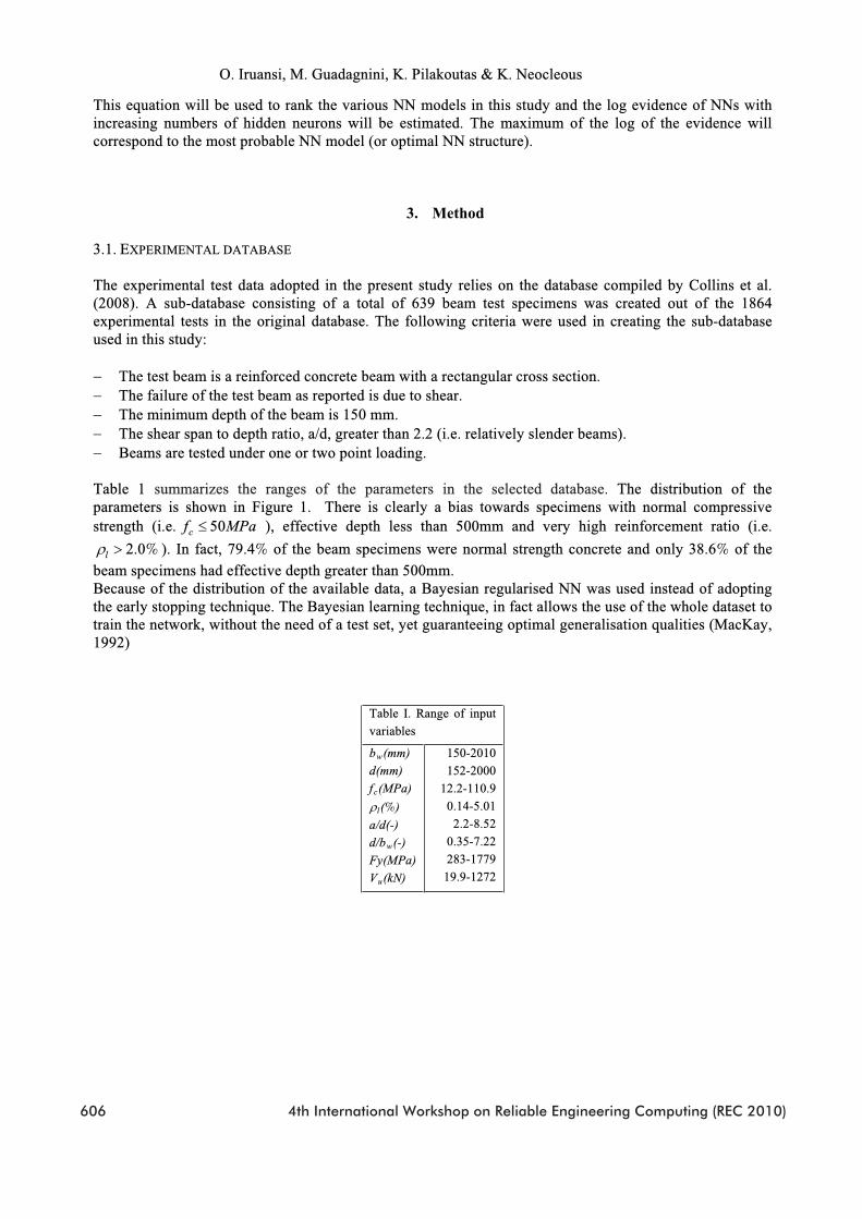
The experimental test data adopted in the present study relies on the database compiled by Collins et al.(2008). A sub-database consisting of a total of 639 beam test specimens was created out of the 1864 experimental tests in the original database. The following criteria were used in creating the sub-database used in this study:

The test beam is a reinforced concrete beam with a rectangular cross section.The failure of the test beam as reported is due to shear.The minimum depth of the beam is 150 mm.The shear span to depth ratio, a/d, greater than 2.2 (i.e. relatively slender beams).Beams are tested under one or two point loading.

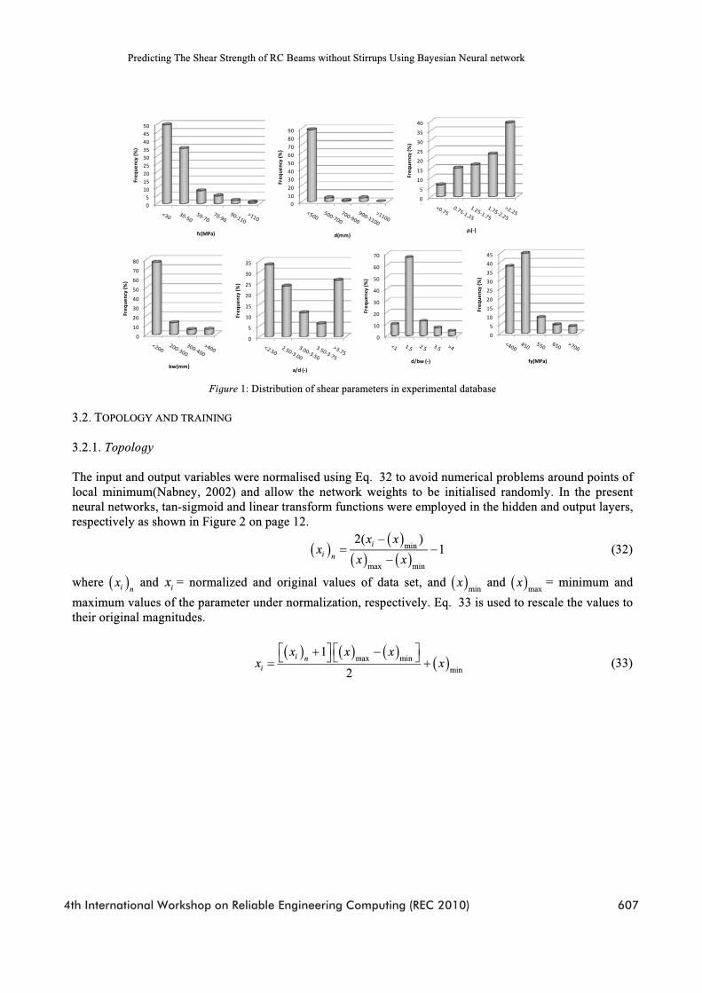
Table 1 summarizes the ranges of the parameters in the selected database. The distribution of the parameters is shown in Figure 1. There is clearly a bias towards specimens with normal compressive strength (i.e. 50cf MPa ), effective depth less than 500mm and very high reinforcement ratio (i.e.

2.0%l ). In fact, 79.4% of the beam specimens were normal strength concrete and only 38.6% of the

beam specimens had effective depth greater than 500mm. Because of the distribution of the available data, a Bayesian regularised NN was used instead of adopting the early stopping technique. The Bayesian learning technique, in fact allows the use of the whole dataset to train the network, without the need of a test set, yet guaranteeing optimal generalisation qualities (MacKay, 1992)

Table I. Range of input

variables

bw(mm)

d(mm)

fc(MPa)

l(%)

a/d(-)

d/bw(-)

Fy(MPa)

Vu

150-2010

(kN)

152-2000

12.2-110.9

0.14-5.01

2.2-8.52

0.35-7.22

283-1779

19.9-1272



0

5

10

15

20

25

30

35

Freq

uenc

y (%

)

a/d (-)

0

10

20

30

40

50

60

70

80

Freq

uenc

y (%

)

bw(mm)

0102030405060708090

Freq

uenc

y (%

)

d(mm)

0

10

20

30

40

50

60

70

Freq

uenc

y (%

)d/bw (-)

05101520253035404550

Freq

uenc

y (%

)

fc(MPa)

0

5

10

15

20

25

30

35

40

45

Freq

uenc

y (%

)

fy(MPa)

0

5

10

15

20

25

30

35

40

Freq

uenc

y (%

)

l(-)

Figure 1: Distribution of shear parameters in experimental database

3.2. TOPOLOGY AND TRAINING

3.2.1. Topology

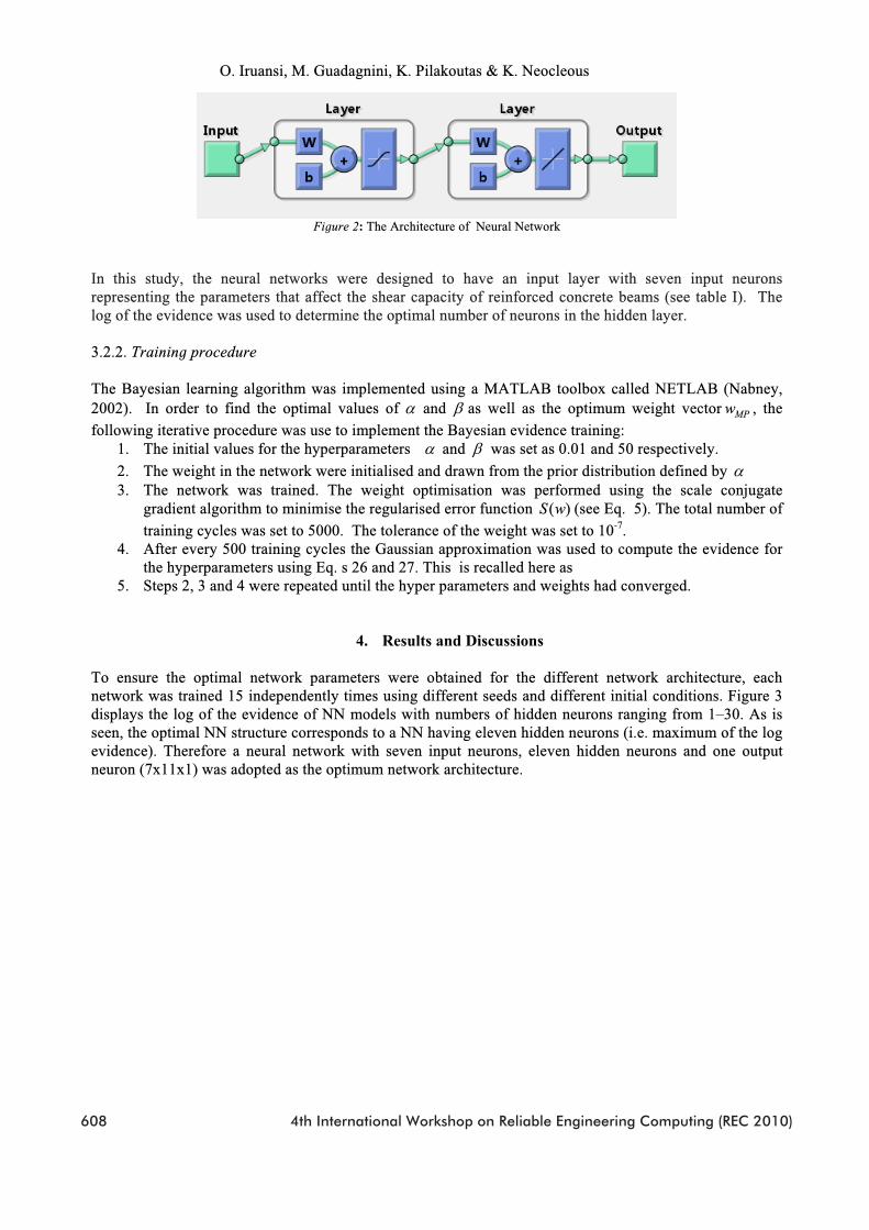
The input and output variables were normalised using Eq. 32 to avoid numerical problems around points of local minimum(Nabney, 2002) and allow the network weights to be initialised randomly. In the present neural networks, tan-sigmoid and linear transform functions were employed in the hidden and output layers, respectively as shown in Figure 2 on page 12.

min

max min

2( )1i

i n

x xx

x x (32)

where i nx and ix = normalized and original values of data set, and

minx and

maxx = minimum and

maximum values of the parameter under normalization, respectively. Eq. 33 is used to rescale the values to their original magnitudes.

max min

min

1

2

i ni

x x xx x (33)



Figure 2: The Architecture of Neural Network

In this study, the neural networks were designed to have an input layer with seven input neuronsrepresenting the parameters that affect the shear capacity of reinforced concrete beams (see table I). The log of the evidence was used to determine the optimal number of neurons in the hidden layer.

3.2.2. Training procedure

The Bayesian learning algorithm was implemented using a MATLAB toolbox called NETLAB (Nabney, 2002). In order to find the optimal values of and as well as the optimum weight vector MPw , the

following iterative procedure was use to implement the Bayesian evidence training:1. The initial values for the hyperparameters and was set as 0.01 and 50 respectively.

2. The weight in the network were initialised and drawn from the prior distribution defined by 3. The network was trained. The weight optimisation was performed using the scale conjugate

gradient algorithm to minimise the regularised error function ( )S w (see Eq. 5). The total number of

training cycles was set to 5000. The tolerance of the weight was set to 10-7

4. After every 500 training cycles the Gaussian approximation was used to compute the evidence for the hyperparameters using Eq. s 26 and 27. This is recalled here as

.

5. Steps 2, 3 and 4 were repeated until the hyper parameters and weights had converged.

4. Results and Discussions

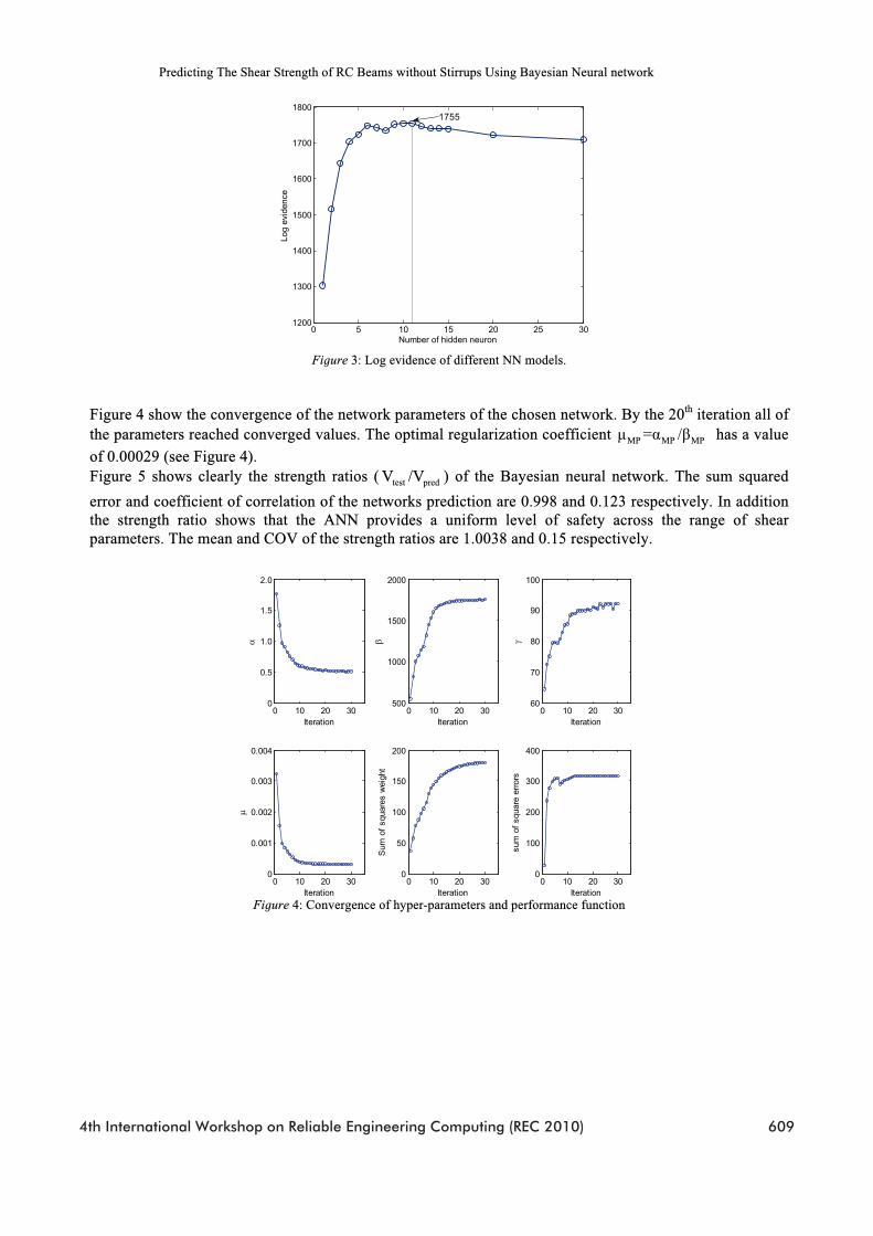
To ensure the optimal network parameters were obtained for the different network architecture, each network was trained 15 independently times using different seeds and different initial conditions. Figure 3displays the log of the evidence of NN models with numbers of hidden neurons ranging from 1–30. As is seen, the optimal NN structure corresponds to a NN having eleven hidden neurons (i.e. maximum of the log evidence). Therefore a neural network with seven input neurons, eleven hidden neurons and one output neuron (7x11x1) was adopted as the optimum network architecture.



0 5 10 15 20 25 301200

1300

1400

1500

1600

1700

1800

Number of hidden neuron

Log e

vidence

1755

Figure 3: Log evidence of different NN models.

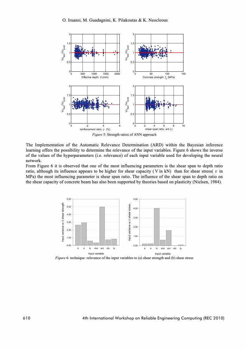
Figure 4 show the convergence of the network parameters of the chosen network. By the 20th

MP MP MP

iteration all of the parameters reached converged values. The optimal regularization coefficient has a value

of 0.00029 (see Figure 4).Figure 5 shows clearly the strength ratios ( test predV /V ) of the Bayesian neural network. The sum squared

error and coefficient of correlation of the networks prediction are 0.998 and 0.123 respectively. In addition the strength ratio shows that the ANN provides a uniform level of safety across the range of shear parameters. The mean and COV of the strength ratios are 1.0038 and 0.15 respectively.

0 10 20 300

0.5

1.0

1.5

2.0

Iteration0 10 20 30

500

1000

1500

2000

Iteration0 10 20 30

60

70

80

90

100

Iteration

0 10 20 300

0.001

0.002

0.003

0.004

Iteration0 10 20 30

0

50

100

150

200

Iteration

Sum

of

squa

res

wei

ght

0 10 20 300

100

200

300

400

Iteration

sum

of

squa

re e

rror

s

Figure 4: Convergence of hyper-parameters and performance function



0 500 1000 1500 20000

0.5

1

1.5

2

Effective depth, d (mm)

Vu te

st/V

u pred

0 50 100 1500

0.5

1

1.5

2

Concrete strength, fc (MPa)

Vu te

st/V

u pred

0 2 4 60

0.5

1

1.5

2

reinforcement ratio, (%)

Vu te

st/V

u pred

0 2 4 6 8 100

0.5

1

1.5

2

shear span ratio, a/d (-)V

u test

/Vu pr

ed

Figure 5: Strength ratios of ANN approach

The Implementation of the Automatic Relevance Determination (ARD) within the Bayesian inference learning offers the possibility to determine the relevance of the input variables. Figure 6 shows the inverse of the values of the hyperparameters (i.e. relevance) of each input variable used for developing the neural network. From Figure 6 it is observed that one of the most influencing parameters is the shear span to depth ratioratio, although its influence appears to be higher for shear capacity ( V in kN) than for shear stress( v in MPa) the most influencing parameter is shear span ratio. The influence of the shear span to depth ratio on the shear capacity of concrete beam has also been supported by theories based on plasticity (Nielsen, 1984).

Input variable

b d fc rhol a/d d/b fy

Inpu

t va

rianc

e w

.r.t

she

ar s

tren

gth

0.00

1.00

2.00

3.00

4.00

5.00

6.00

Input variable

b d fc rhol a/d d/b fy

Inpu

t va

rianc

e w

.r.t

she

ar s

tres

s

0.00

1.00

2.00

3.00

4.00

5.00

Figure 6: technique: relevance of the input variables to (a) shear strength and (b) shear stress



4.6. SIMULATION OF SHEAR STRENGTH OF RC BEAMS

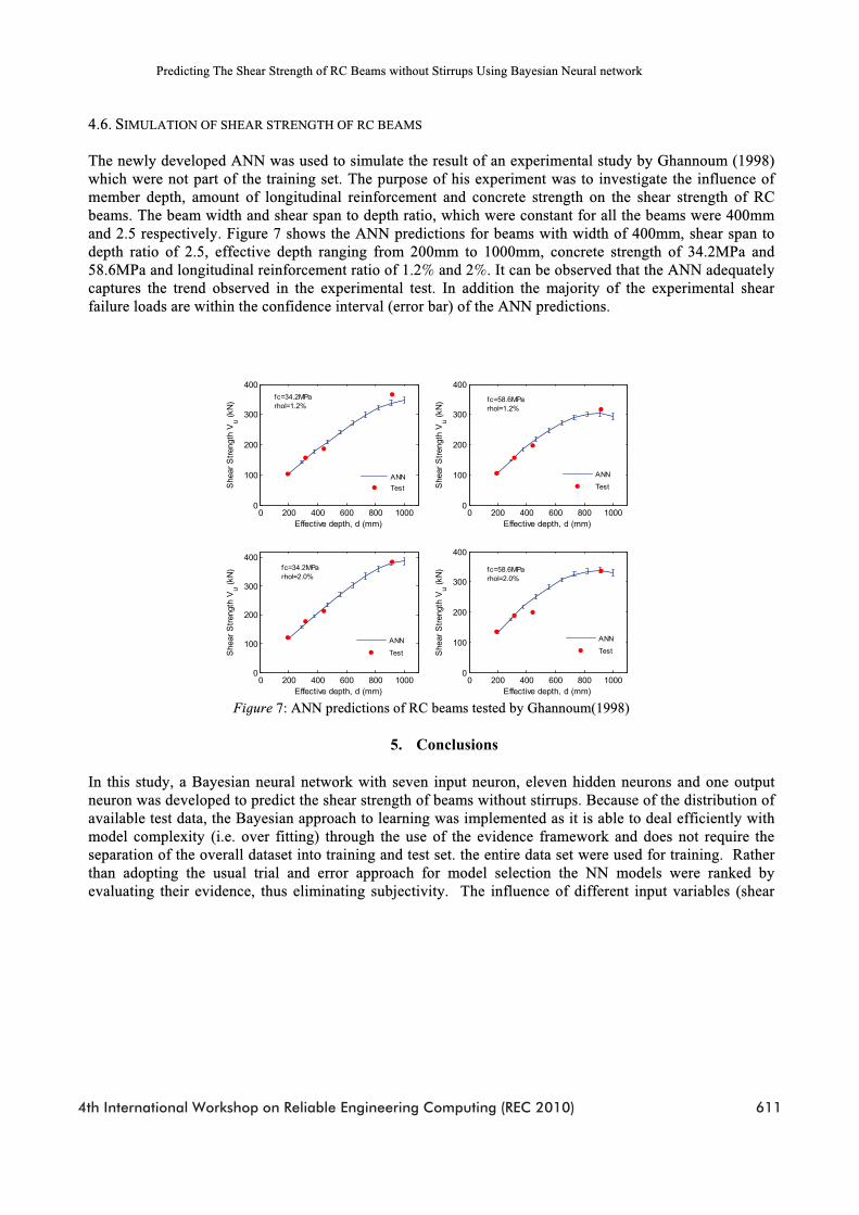
The newly developed ANN was used to simulate the result of an experimental study by Ghannoum (1998)which were not part of the training set. The purpose of his experiment was to investigate the influence of member depth, amount of longitudinal reinforcement and concrete strength on the shear strength of RC beams. The beam width and shear span to depth ratio, which were constant for all the beams were 400mmand 2.5 respectively. Figure 7 shows the ANN predictions for beams with width of 400mm, shear span to depth ratio of 2.5, effective depth ranging from 200mm to 1000mm, concrete strength of 34.2MPa and 58.6MPa and longitudinal reinforcement ratio of 1.2% and 2%. It can be observed that the ANN adequately captures the trend observed in the experimental test. In addition the majority of the experimental shear failure loads are within the confidence interval (error bar) of the ANN predictions.

0 200 400 600 800 10000

100

200

300

400


She

ar S

tren

gth

Vu (

kN)

0 200 400 600 800 10000

100

200

300

400


She

ar S

tren

gth

Vu (

kN)

0 200 400 600 800 10000

100

200

300

400


She

ar S

tren

gth

Vu (

kN)

0 200 400 600 800 10000

100

200

300

400


She

ar S

tren

gth

Vu (

kN)

ANN

Test

ANN

Test

ANN

Test

ANN

Test

fc=34.2MParhol=1.2%

fc=58.6MParhol=1.2%

fc=34.2MParhol=2.0%

fc=58.6MParhol=2.0%

Figure 7: ANN predictions of RC beams tested by Ghannoum(1998)

5. Conclusions

In this study, a Bayesian neural network with seven input neuron, eleven hidden neurons and one output neuron was developed to predict the shear strength of beams without stirrups. Because of the distribution of available test data, the Bayesian approach to learning was implemented as it is able to deal efficiently with model complexity (i.e. over fitting) through the use of the evidence framework and does not require the separation of the overall dataset into training and test set. the entire data set were used for training. Rather than adopting the usual trial and error approach for model selection the NN models were ranked by evaluating their evidence, thus eliminating subjectivity. The influence of different input variables (shear



parameters) on the shear strength was evaluated. The study showed that within the range of input parameters used to train the network, the predictions of the ANN provide a uniform level of safety.The application of the neural network to RC beams specimens which were not part of the training showed that the network is capable of simulating the effect of various parameters on the shear strength. Finally thisstudy showed the potential of using Neural Networks as an alternative method for predicting the strength strength of RC beams and investigating the effect of the many variables on the shear strength as well as their complete interaction.

Reference

BISHOP, C. M. 1995. Neural networks for pattern recognition, Oxford, Oxford University Press.CLADERA, A. & MARI, A. R. 2004. Shear Design procedure for Reinforced Normal and High

Strength Concrete Beams using Artificial Neural Networks. Part 1: Beams without Stirrups. Engineering Structures, 26, 917-926.

COLLINS, M. P., BENTZ, E. C. & SHERWOOD, E. G. 2008. Where is Shear Reinforcement Required? A Review of Research Results and Design Procedures. ACI Structural Journal, 105.

EL CHABIB, H., NEHDI, M. & SAÏD, A. 2006. Predicting the effect of stirrups on shear strength of reinforced normal-strength concrete (NSC) and high-strength concrete (HSC) slender beams using artificial intelligence. Canadian Journal of Civil Engineering, 33, 933-944.

GOH, A. T. C. 1995. Prediction of ultimate shear strength of deep beams using neural networks. ACI Structural Journal, 92, 28-32.

GOH, A. T. C., KULHAWY, F. H. & CHUA, C. G. 2005. Bayesian Neural Network Analysis of Undrained Side Resistance of Drilled Shafts. JOURNAL OF GEOTECHNICAL AND GEOENVIRONMENTAL ENGINEERING, 131, 84-93.

HSU, C.-T. T. 1988. Softened truss model theory for shear and torsion. ACI Structural Journal, 85,624-35.

IRUANSI, O., GUADAGNINI, M. & PILAKOUTAS, K. 2009. Design Provisions for Large and Lightly RC beams. Concrete Comunication Symposium. Leeds: The Concrete Centre.

K. H. YANG, A. F. ASHOUR, SONG, J. K. & LEE, E.-T. 2008. Neural Network Modelling for Shear Strength of Reinforced Concrete Deep Beams. Structures & Buildings, 161, 29-39.

MACKAY, D. J. C. 1992. A practical Bayesian framework for back-propagation networks. Neural Computation, 4, 448-72.

MANSOUR, M. Y., DICLELI, M., LEE, J. Y. & ZHANG, J. 2004. Predicting the shear strength of reinforced concrete beams using artificial neural networks Engineering Structures, 26, 781-799.

NABNEY, I. T. 2002. NETLAB: Algorithms for pattern recognition, London, Springer.NEAL, R. M. 1992. Bayesian Learning for Neural Networks. PhD Ph.D. thesis, University of Toronto.NIELSEN, M. P. 1984. Limit State Analysis and concrete plasticity, Englewood Cliffs, N.J., Prentice-

hall.ORETA, A. W. 2004. Simulating size effect on shear strength of RC beams without stirrups using

neural networks Engineering Structures, 26, 681-691 SANAD, A. & SAKA, M. P. 2001. Shear Strength of Reinforced-Concrete Deep Beams using Neural

Networks. Journal of Structural Engineering, 127, 818-828.SELEEMAH, A. A. 2005. A neural network model for predicting maximum shear capacity of concrete

beams without transverse reinforcementCanadian Journal of Civil Engineering, 32, 644–657



VECCHIO, F. J. & COLLINS, M. P. 1986. The Modified Compression Field Theory for Reinforced Concrete Elements Subjected to Shear. ACI Journal, 83, 219-231.

YANG, K. H., ASHOUR, A. F. & SONG, J. K. 2007. Shear Capacity of Reinforced Concrete Beams using Neural network. International Journal of Concrete Structures and Materials, 1, 63-73.


Predicting the Shear Strength of RC Beams without Stirrups ... · Predicting the Shear Strength of...

Documents

Transcript of Predicting the Shear Strength of RC Beams without Stirrups ... · Predicting the Shear Strength of...