Predicting the Performance of Contestants in Competitive ...

Olympiads in Informatics, 2020, Vol. 14, 3–20© 2020 IOI, Vilnius UniversityDOI: 10.15388/ioi.2020.01

3

Predicting the Performance of Contestants in Competitive Programming Using Machine Learning Techniques

Ammar ALNAHHAS, Nour MOURTADA Faculty of information technology engineeringDamascus University – Damascus – Syriae-mail: [email protected], [email protected]

Abstract. Training is an important task in competitive programming, coaches can improve the training experience if they can get information about the performance of contestants. In this paper, we study the possibility of using machine learning techniques to build a system that is able to predict the future performance of a contestant by analyzing their historical rating list. This system learns from a dataset of contestant ratings. We propose to apply five different baseline machine learning techniques, then we propose a new deep learning model. We conduct an experiment us-ing public data from the Codeforces website. We show that most techniques achieve acceptable results. In addition, the proposed deep learning model outperformed all baseline methods and achieved results that proved its efficiency in predicting the future performance of contestants. This paper confirms the possibility of using machine learning techniques to help in the process of preparing contestants in competitive programming.

Keywords: competitive programming, machine learning, artificial intelligence, programming training, Informatics Olympiads.

1. Introduction

Competitive programming has become very popular in recent years. It has been attract-ing more interest all over the world. Many important competitions in competitive pro-gramming are organized each year, such as the International Olympiad in Informatics (IOI) and the International Collegiate Programming Contest (ICPC). Thousands of con-testants are participating in competitive programming competitions that are held online and onsite all over the world.

Training is a key element in preparing for competitive programming, therefore, many institutions like organizers of national Olympiads in informatics and universities are interested in creating and adopting successful training plans for their contestants (Combéfis & Paques, 2015), and many training methods are introduced and discussed.

A. Alnahhas, N. Mourtada4

Because of the importance of the training, many coaches follow up with their contes-tants to support their training process and provide suitable materials and tools. For this reason, it is important for coaches and people in charge of training to observe and track contestant performance. It is useful if they have an indicator if the performance of a contestant is decreasing, so they can help in the early stage and support the con-testant.

Artificial intelligence has gained more interest in both research and application in the recent years, it is becoming part of everyday life, many intelligent applications are helping people doing their work, and it has been used in modern educational systems to make them more adaptive for learners (Colchester, Hagras, Alghazzawi, & Aldab-bagh, 2017), machine learning is one of the most interesting branches of artificial intel-ligence, this field of science is interested in building intelligent systems that can learn by itself, usually by observing and analyzing a large amount of available data.

As thousands of contestants are now interested in competitive programming, online training websites like Codeforces provide large amounts of contestant data, so it is pos-sible to build an intelligent system to help analyze this data and support the training process using artificial intelligence.

In this paper, we are going to present a methodology that aims at using machine learning techniques in order to build a system that can predict the future performance of competitive programming contestants by analyzing a sequence of their historical rat-ings. We implement some known machine learning models, then we propose a new deep learning model and prove its efficacy in tracking contestants’ performance by providing results of empirical experiments on data from Codeforces.

Although coaches can observe their contestants to ensure their performance is not going to decrease, there are some reasons an automatic system can support this pro-cess:

The relation between contestant performance and their historical ratings may be ●not simple to be detected by humans. Complex patterns may exist in this case. Computer systems can detect these patterns especially using machine learning techniques by analyzing big amount of data, and extracting useful information by generalization.The number of contestants may be large for coaches to follow up in some cases, ●so an automatic system can help by pointing the coaches to potential performance-decreasing contestants, so that they can do further observations and check the situation.

Therefore, the proposed system can be seen as a decision support system that helps coaches during the training process by providing an early alarm, so that they can act in a timely manner. This system can help coaches of national Olympiads where number of contestants participating in the training process may be large.

This paper is organized as follows: section 2 provides some related works in the field of predicting student performance, section 3 presents a formal description of the prob-lem we are trying to solve, section 4 introduces the baseline machine learning models application, section 5 proposes a new deep learning model, section 6 contains the details and results of the experiments, and finally section 7 concludes this paper.

Predicting the Performance of Contestants in Competitive Programming ... 5

2. Related Work

Although no researchers have tried to predict the performance of contestants in competi-tive programming using artificial intelligence techniques; much research has focused on using related methodologies to predict school or university student performance as well as detecting students with poor educational progress. This research varied in the way they addressed and solved the problem. Some of them used traditional machine learning techniques, while others tried to use deep learning methods such as convolutional and recurrent neural networks.

Kotsiantis, Pierrakeas, & Pintelas (2004) proposed to use various machine learning algorithms to predict the performance of students in a distance learning environment, they used a dataset that consists of students in an informatic course. The students were represented by two types of attributes: demographic and performance. Five different machine learning techniques were applied to predict if a student would succeed or fail in the final exam. The results showed that the Naïve Bayes algorithm achieved the best results. Tanner & Toivonen (2010) tried to predict students’ final exam results in an online touch-typing course in which each student had to pass 12 lessons and a final exam. The goal of the research was to predict in early stages of the course if a student was going to fail the exam so that the teachers could provide more tutoring. The researchers suggested using the K-nearest neighbors (KNN) algorithm, a machine learning technique that depends on the idea that students with similar attributes tend to have similar exam results. The authors reported good results using KNN in predicting student performance. Tan & Shao (2015) presented a machine learning-based system that helped predict student dropout in an educational system. They argued that the per-formance of the students is an important factor of dropout, so they suggested building a binary classifier that can predict if a student will drop out or graduate eventually. The proposed system used the grades of each student as input, and applied two differ-ent algorithms to analyze the data: logistic regression and decision trees. The authors showed that both methods achieved good results. Amra & Maghari (2017) proposed a system that can predict secondary students’ future performance based on various attri-butes. They compared two different machine learning algorithms: K-nearest neighbors and the Naïve Bayes classifier. The results they presented showed that the Naïve Bayes model achieved higher accuracy. Babić (2017) presented a system that aimed at pre-dicting student academic motivation. The proposed system depended on the behavior of students in an online learning management system, and used three different machine learning methods to classify students: artificial neural networks (ANN), decision trees and support vector machines. The results were promising and could help educators find students with poor performance at early stages. Waheed et al. (2020) tried to build a system that can predict the academic performance of students in a virtual learning envi-ronment based on clickstream data and assessment results. Their system used artificial neural networks to categorize students into two classes: success and failure. Authors compared the results with baseline methods: logistic regression and support vector ma-chines, and proved that ANN outperformed them. Similarly, researchers Hussain et al. (2019) proposed to use artificial neural networks to predict student performance based


on internal assessment results. They presented the issue as a classification problem, as other researchers did, but they compared the results of ANN with two different classi-fiers: The Artificial Immune Recognition System and AdaBoost. The proposed model used exam scores and internal assessment marks; the results showed that ANN out-performed other methods. Sekeroglu, Dimililer, & Tuncal (2019) also used neural net-works to predict student performance. They suggested two different neural networks, multilayer perceptron (MLP) and recurrent neural networks, and compared the perfor-mance of these two networks with support vector machines. MLP proved to be best at classifying students and predicting performance. Koutina & Kermanidis (2011) tried to build a system to predict the performance of postgraduate students in order to help tutors detect students at risk of failing in early stages. The authors used students’ marks along with some demographic attributes to predict the performance and compared six well-known machine learning algorithms including support vector machines, Naïve Bayes and K-nearest neighbor. Their research led to the result that the Naive Bayes classifier achieved the best results.

Many other researchers were interested in this field (Al-Shabandar et al., 2017; Ofori, Maina, & Gitonga, 2020; Thai-Nghe, Drumond, Krohn-Grimberghe, & Schmidt-Thie-me, 2010; Xu, Moon, & Van Der Schaar, 2017). The successful use of machine learning and deep learning techniques to predict the performance of students in the previous work is a good indicator that these methods can help predict the performance of contestants in competitive programming. Especially as many researchers use a similar input pattern which is the sequence of level rates of the contestant. We are going to apply different well-known traditional machine learning techniques along with a new deep learning model to try to achieve the research goal.

3. Formal Problem Statement

The problem we present in this paper is about predicting the future performance of a contestant participating in a competitive programming training program. Each contes-tant is assumed to have a rate that reflects their excellence level, which changes over time to reflect change in contestant performance. The goal is to predict if the level of the contestant is going to increase or decrease according to the historical ratings we already recorded for them.

We can measure the performance of a contestant by the average of their level ratings, so if the average increases over time, then we can say that the student performance is getting better and vice versa.

Formally, if a contestant c has a sequence of n temporally ordered ratings R = r1, r2, …, rn, we define the function RC(R) as the following:

𝑅𝐶(𝑅) = 1𝑛 2⁄ � 𝑟�

�=𝑛

�=𝑛/2− 1𝑛 2⁄ � 𝑟�

𝑛/2−1

�=1


The function RC denotes the difference in rating average between the first half and the second half of the rating sequence. Intuitively, if the function RC has a positive value, the contestant performance is increasing while a negative value means the performance is decreasing, and this is the case we are interested in, because detecting contestants who tend to do worse in the future will guide the coaches to provide suitable solutions.Formally, we define the function T(R) as the following:

𝑅𝐶(𝑅) = 1𝑛 2⁄ � 𝑟�

�=𝑛

�=𝑛/2− 1𝑛 2⁄ � 𝑟�

𝑛/2−1

�=1

𝑇(𝑅) = �1, 𝑅𝐶(𝑅) < 00, 𝑅𝐶(𝑅) ≥ 0

So, the goal of the models in this paper is to predict the value of T(R) given n/2 ratings of a contestant. As the value of T(R) is binary, the problem can be addressed as a binary classification, that is, each sequence of ratings belongs to either a positive or negative class. Binary classification problems are well-known to be solved by many ma-chine learning and deep learning methods that can be trained using a dataset of existing instances, so the model can generalize and classify new instances of data.

To solve the proposed classification problem, we will apply different types of baseline machine learning algorithms, then present a novel deep learning model that achieves good results and outperforms all other methods, as we will elaborate in the results section.

4. Baseline Machine Learning Algorithms

Machine learning is used to discover data patterns and relationships between variables, which is helpful in the decision-making process. It is a useful tool for detecting contes-tants whose level is going to decrease based on their rating sequence. Coaches are then able to help the weakest ones in a timely manner, and to promote the strongest, thereby improving contestants’ level. There are several well-known machine learning models that are usually used in classification tasks. We choose five of them to apply in our study, and will provide a brief description of how we apply them in this section.

4.1. Random Forest

Random forest (Liaw & Wiener, 2002) is a classification methodology widely used in machine learning. Random forest is a collection of decision trees (Quinlan, 1986) built up with some element of random choice. Each decision tree is constructed using ran-dom features of the data. The trees are not pruned, and each leaf of each tree represents a class. The algorithm is trained using a bootstrap sampling method. The prediction of a new item is done by the voting technique, that is, the prediction of each tree is found according to the leaf reached, then each class is assigned a ratio of trees that voted for it. The random forest algorithm has been successfully used in many applications; in our


case we construct the forest using our dataset. We build trees from the ratings of the con-testants, and the forest we construct contains 100 decision trees. We use Gini impurity as a criterion for splitting tree nodes.

4.2. Logistic Regression

Logistic regression is a binary classification model. It is considered as a baseline for any binary classification problem, and is a basic fundamental concept in machine learn-ing. It describes data and estimates the relation between one dependent binary variable and independent variables. It is a special case of linear regression where the dependent binary variable is categorical in nature. Linear regression gives a continuous output, but logistic regression gives a constant output. Logistic regression is suitable for our goal, where the dependent variable is the contestant class or performance prediction, and the independent variables are the historical ratings of this contestant. Given the rating se-quence R = r1, r2, …, rn of a contestant, we define a linear function Z:

𝑅𝐶(𝑅) = 1𝑛 2⁄ � 𝑟�

�=𝑛

�=𝑛/2− 1𝑛 2⁄ � 𝑟�

𝑛/2−1

�=1

𝑇(𝑅) = �1, 𝑅𝐶(𝑅) < 00, 𝑅𝐶(𝑅) ≥ 0

𝑍(𝑅) = 𝛽0 + 𝛽1𝑟1 + 𝛽2𝑟2 + ⋯+ 𝛽𝑛𝑟𝑛

The factors

𝑅𝐶(𝑅) = 1𝑛 2⁄ � 𝑟�

�=𝑛

�=𝑛/2− 1𝑛 2⁄ � 𝑟�

𝑛/2−1

�=1

𝑇(𝑅) = �1, 𝑅𝐶(𝑅) < 00, 𝑅𝐶(𝑅) ≥ 0

𝑍(𝑅) = 𝛽0 + 𝛽1𝑟1 + 𝛽2𝑟2 + ⋯+ 𝛽𝑛𝑟𝑛

𝛽0,𝛽1,𝛽2, … ,𝛽𝑛 are the model parameters whose value should be found by the model fitting process.

We apply a logistic function L to the result of the above function to get the value in the range (0,1):

𝑅𝐶(𝑅) = 1𝑛 2⁄ � 𝑟�

�=𝑛

�=𝑛/2− 1𝑛 2⁄ � 𝑟�

𝑛/2−1

�=1

𝑇(𝑅) = �1, 𝑅𝐶(𝑅) < 00, 𝑅𝐶(𝑅) ≥ 0

𝑍(𝑅) = 𝛽0 + 𝛽1𝑟1 + 𝛽2𝑟2 + ⋯+ 𝛽𝑛𝑟𝑛

𝛽0,𝛽1,𝛽2, … ,𝛽𝑛

𝐿(𝑅) = 11 − 𝑒−𝑍(𝑅)

The function L represents the output of the model, and the predicted class is then found by choosing a suitable threshold th and find the class accordingly:

𝑅𝐶(𝑅) = 1𝑛 2⁄ � 𝑟�

�=𝑛

�=𝑛/2− 1𝑛 2⁄ � 𝑟�

𝑛/2−1

�=1

𝑇(𝑅) = �1, 𝑅𝐶(𝑅) < 00, 𝑅𝐶(𝑅) ≥ 0

𝑍(𝑅) = 𝛽0 + 𝛽1𝑟1 + 𝛽2𝑟2 + ⋯+ 𝛽𝑛𝑟𝑛

𝛽0,𝛽1,𝛽2, … ,𝛽𝑛

𝐿(𝑅) = 11 − 𝑒−𝑍(𝑅)

𝑐𝑙𝑎𝑠𝑠 = �0, 𝐿(𝑅) < 𝑡ℎ1, 𝐿(𝑅) ≥ 𝑡ℎ

The training of the model is done by minimizing the mean squared error between the function L of the model and the real output of the training samples.

4.3. Artificial Neural Networks

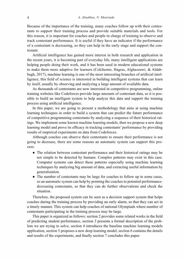
A neural network consists of connected items called neurons, where each neuron has multiple inputs and a single output. There are many types of neural networks which vary in the way the neurons are connected to each other. Multilayer perceptron (MLP) is one of the famous types of neural networks. In MLP neurons are arranged in consecutive layers where the output of neurons of each layer constitutes the input of the next layer.


The first layer is the input layer, and the last layer is the output layer whose output is considered the output of the whole network. MLP is used widely in machine learning as it can learn from existing samples of data and generalize the pattern to be applied to new items, so it is useful in various classification and regression tasks. In our work, we use MLP as a binary classifier; we use a three-layer MLP. The first layer is the input layer which consists of neurons where each neuron corresponds to a rating from the input, the second layer is a hidden layer and the third layer is the output layer which consists of a single neuron. Fig. 1 shows the network architecture. The activation function for the first and second layers is the ReLU function, which is a positive linear function, whereas the activation function of the output layer is sigmoid:

𝑅𝐶(𝑅) = 1𝑛 2⁄ � 𝑟𝑖

𝑖=𝑛

𝑖=𝑛/2− 1𝑛 2⁄ � 𝑟𝑖

𝑛/2−1

𝑖=1

𝑇(𝑅) = �1, 𝑅𝐶(𝑅) < 00, 𝑅𝐶(𝑅) ≥ 0

𝑍(𝑅) = 𝛽0 + 𝛽1𝑟1 + 𝛽2𝑟2 + ⋯+ 𝛽𝑛𝑟𝑛

𝛽0,𝛽1,𝛽2, … ,𝛽𝑛

𝐿(𝑅) = 11 − 𝑒−𝑍(𝑅)

𝑐𝑙𝑎𝑠𝑠 = �0, 𝐿(𝑅) < 𝑡ℎ1, 𝐿(𝑅) ≥ 𝑡ℎ

𝑆𝑖𝑔𝑚𝑜𝑖𝑑(𝑥) = 11 + 𝑒−𝑥

The output of the Sigmoid function is in range (0,1). To get the final class we choose a suitable threshold th and find the class accordingly:

𝑅𝐶(𝑅) = 1𝑛 2⁄ � 𝑟𝑖

𝑖=𝑛

𝑖=𝑛/2− 1𝑛 2⁄ � 𝑟𝑖

𝑛/2−1

𝑖=1

𝑇(𝑅) = �1, 𝑅𝐶(𝑅) < 00, 𝑅𝐶(𝑅) ≥ 0

𝑍(𝑅) = 𝛽0 + 𝛽1𝑟1 + 𝛽2𝑟2 + ⋯+ 𝛽𝑛𝑟𝑛

𝛽0,𝛽1,𝛽2, … ,𝛽𝑛

𝐿(𝑅) = 11 − 𝑒−𝑍(𝑅)

𝑐𝑙𝑎𝑠𝑠 = �0, 𝐿(𝑅) < 𝑡ℎ1, 𝐿(𝑅) ≥ 𝑡ℎ


𝑐𝑙𝑎𝑠𝑠 = �0, 𝑜𝑢𝑡𝑝𝑢𝑡 < 𝑡ℎ1, 𝑜𝑢𝑡𝑝𝑢𝑡 ≥ 𝑡ℎ

To train the network we use the Adam algorithm (Kingma & Ba, 2014) and cross entropy as a loss function.

. . . .

. . . .

Contestant's rating list

Output

Fig. 1. Proposed MLP architecture.


4.4. Naïve Bayes Classifier

The Naive Bayes algorithm is an effective and efficient classification method in machine learning. A Naive Bayes classifier is a simple probabilistic classifier based on applying Bayes’ theorem with strong (naive) independence assumptions. Bayes’ theorem depends on the following relationship, given class variable y which denotes contestant perfor-mance prediction and the dependent feature vector, which is the historical ratings of this contestant r1 through rn:

𝑅𝐶(𝑅) = 1𝑛 2⁄ � 𝑟𝑖

𝑖=𝑛

𝑖=𝑛/2− 1𝑛 2⁄ � 𝑟𝑖

𝑛/2−1

𝑖=1

𝑇(𝑅) = �1, 𝑅𝐶(𝑅) < 00, 𝑅𝐶(𝑅) ≥ 0

𝑍(𝑅) = 𝛽0 + 𝛽1𝑟1 + 𝛽2𝑟2 + ⋯+ 𝛽𝑛𝑟𝑛

𝛽0,𝛽1,𝛽2, … ,𝛽𝑛

𝐿(𝑅) = 11 − 𝑒−𝑍(𝑅)

𝑐𝑙𝑎𝑠𝑠 = �0, 𝐿(𝑅) < 𝑡ℎ1, 𝐿(𝑅) ≥ 𝑡ℎ



𝑃(𝑟, … . , 𝑟𝑛) = 𝑃(𝑦)𝑃(𝑟1, … , 𝑟𝑛|𝑦)𝑃(𝑟1, … . . , 𝑟𝑛)

To train our model, we use two different methods. Firstly, we train a Gaussian Naïve Bayes Model which implements the Gaussian Naive Bayes algorithm for classification. Gaussian Naïve Bayes theorem states the following relationship:

𝑅𝐶(𝑅) = 1𝑛 2⁄ � 𝑟𝑖

𝑖=𝑛

𝑖=𝑛/2− 1𝑛 2⁄ � 𝑟𝑖

𝑛/2−1

𝑖=1

𝑇(𝑅) = �1, 𝑅𝐶(𝑅) < 00, 𝑅𝐶(𝑅) ≥ 0

𝑍(𝑅) = 𝛽0 + 𝛽1𝑟1 + 𝛽2𝑟2 + ⋯+ 𝛽𝑛𝑟𝑛

𝛽0,𝛽1,𝛽2, … ,𝛽𝑛

𝐿(𝑅) = 11 − 𝑒−𝑍(𝑅)

𝑐𝑙𝑎𝑠𝑠 = �0, 𝐿(𝑅) < 𝑡ℎ1, 𝐿(𝑅) ≥ 𝑡ℎ




𝑃(𝑦) = 1�2𝜋𝜎𝑦2

exp� −�𝑟𝑖 − 𝜇𝑦�

2

2𝜎𝑦2�

Secondly, we train a Multinomial Naïve Bayes Model which implements the naive Bayes algorithm for multinomial distributed data. The distribution is parametrized by vectors

𝑅𝐶(𝑅) = 1𝑛 2⁄ � 𝑟𝑖

𝑖=𝑛

𝑖=𝑛/2− 1𝑛 2⁄ � 𝑟𝑖

𝑛/2−1

𝑖=1

𝑇(𝑅) = �1, 𝑅𝐶(𝑅) < 00, 𝑅𝐶(𝑅) ≥ 0

𝑍(𝑅) = 𝛽0 + 𝛽1𝑟1 + 𝛽2𝑟2 + ⋯+ 𝛽𝑛𝑟𝑛

𝛽0,𝛽1,𝛽2, … ,𝛽𝑛

𝐿(𝑅) = 11 − 𝑒−𝑍(𝑅)

𝑐𝑙𝑎𝑠𝑠 = �0, 𝐿(𝑅) < 𝑡ℎ1, 𝐿(𝑅) ≥ 𝑡ℎ




𝑃(𝑦) = 1�2𝜋𝜎𝑦2


2

2𝜎𝑦2�

𝜃𝑦 = ( 𝜃𝑦1,𝜃𝑦2, … ., 𝜃𝑦𝑛) for each class y.Where:

● n is the number of ratings. ●

𝑅𝐶(𝑅) = 1𝑛 2⁄ � 𝑟𝑖

𝑖=𝑛

𝑖=𝑛/2− 1𝑛 2⁄ � 𝑟𝑖

𝑛/2−1

𝑖=1

𝑇(𝑅) = �1, 𝑅𝐶(𝑅) < 00, 𝑅𝐶(𝑅) ≥ 0

𝑍(𝑅) = 𝛽0 + 𝛽1𝑟1 + 𝛽2𝑟2 + ⋯+ 𝛽𝑛𝑟𝑛

𝛽0,𝛽1,𝛽2, … ,𝛽𝑛

𝐿(𝑅) = 11 − 𝑒−𝑍(𝑅)

𝑐𝑙𝑎𝑠𝑠 = �0, 𝐿(𝑅) < 𝑡ℎ1, 𝐿(𝑅) ≥ 𝑡ℎ




𝑃(𝑦) = 1�2𝜋𝜎𝑦2


2

2𝜎𝑦2�

𝜃𝑦 = ( 𝜃𝑦1,𝜃𝑦2, … ., 𝜃𝑦𝑛)

𝜃𝑦𝑖

is the probability

𝑅𝐶(𝑅) = 1𝑛 2⁄ � 𝑟𝑖

𝑖=𝑛

𝑖=𝑛/2− 1𝑛 2⁄ � 𝑟𝑖

𝑛/2−1

𝑖=1

𝑇(𝑅) = �1, 𝑅𝐶(𝑅) < 00, 𝑅𝐶(𝑅) ≥ 0

𝑍(𝑅) = 𝛽0 + 𝛽1𝑟1 + 𝛽2𝑟2 + ⋯+ 𝛽𝑛𝑟𝑛

𝛽0,𝛽1,𝛽2, … ,𝛽𝑛

𝐿(𝑅) = 11 − 𝑒−𝑍(𝑅)

𝑐𝑙𝑎𝑠𝑠 = �0, 𝐿(𝑅) < 𝑡ℎ1, 𝐿(𝑅) ≥ 𝑡ℎ




𝑃(𝑦) = 1�2𝜋𝜎𝑦2


2

2𝜎𝑦2�

𝜃𝑦 = ( 𝜃𝑦1,𝜃𝑦2, … ., 𝜃𝑦𝑛)

𝜃𝑦𝑖

𝑃(𝑟|𝑦) of rating i appearing in a sample belonging to class y.

Multinomial Naïve Bayes theorem states the following relationship:

𝑅𝐶(𝑅) = 1𝑛 2⁄ � 𝑟𝑖

𝑖=𝑛

𝑖=𝑛/2− 1𝑛 2⁄ � 𝑟𝑖

𝑛/2−1

𝑖=1

𝑇(𝑅) = �1, 𝑅𝐶(𝑅) < 00, 𝑅𝐶(𝑅) ≥ 0

𝑍(𝑅) = 𝛽0 + 𝛽1𝑟1 + 𝛽2𝑟2 + ⋯+ 𝛽𝑛𝑟𝑛

𝛽0,𝛽1,𝛽2, … ,𝛽𝑛

𝐿(𝑅) = 11 − 𝑒−𝑍(𝑅)

𝑐𝑙𝑎𝑠𝑠 = �0, 𝐿(𝑅) < 𝑡ℎ1, 𝐿(𝑅) ≥ 𝑡ℎ




𝑃(𝑦) = 1�2𝜋𝜎𝑦2


2

2𝜎𝑦2�

𝜃𝑦 = ( 𝜃𝑦1,𝜃𝑦2, … ., 𝜃𝑦𝑛)

𝜃𝑦𝑖

𝑃(𝑟|𝑦)

𝜃𝑦𝑖 = 𝑁𝑦𝑖+∝𝑁𝑦+∝ 𝑛

Where:

●

𝑅𝐶(𝑅) = 1𝑛 2⁄ � 𝑟𝑖

𝑖=𝑛

𝑖=𝑛/2− 1𝑛 2⁄ � 𝑟𝑖

𝑛/2−1

𝑖=1

𝑇(𝑅) = �1, 𝑅𝐶(𝑅) < 00, 𝑅𝐶(𝑅) ≥ 0

𝑍(𝑅) = 𝛽0 + 𝛽1𝑟1 + 𝛽2𝑟2 + ⋯+ 𝛽𝑛𝑟𝑛

𝛽0,𝛽1,𝛽2, … ,𝛽𝑛

𝐿(𝑅) = 11 − 𝑒−𝑍(𝑅)

𝑐𝑙𝑎𝑠𝑠 = �0, 𝐿(𝑅) < 𝑡ℎ1, 𝐿(𝑅) ≥ 𝑡ℎ




𝑃(𝑦) = 1�2𝜋𝜎𝑦2


2

2𝜎𝑦2�

𝜃𝑦 = ( 𝜃𝑦1, 𝜃𝑦2, … ., 𝜃𝑦𝑛)

𝜃𝑦𝑖

𝑃(𝑟|𝑦)


𝑁𝑦𝑖 = ∑ 𝑟𝑖𝑟∈𝑇

𝑁𝑦 = ∑ 𝑁𝑦𝑖 𝑛𝑖=1 .

is the number of times rating appears in a sample of class in the training set . ●

𝑅𝐶(𝑅) = 1𝑛 2⁄ � 𝑟𝑖

𝑖=𝑛

𝑖=𝑛/2− 1𝑛 2⁄ � 𝑟𝑖

𝑛/2−1

𝑖=1

𝑇(𝑅) = �1, 𝑅𝐶(𝑅) < 00, 𝑅𝐶(𝑅) ≥ 0

𝑍(𝑅) = 𝛽0 + 𝛽1𝑟1 + 𝛽2𝑟2 + ⋯+ 𝛽𝑛𝑟𝑛

𝛽0,𝛽1,𝛽2, … ,𝛽𝑛

𝐿(𝑅) = 11 − 𝑒−𝑍(𝑅)

𝑐𝑙𝑎𝑠𝑠 = �0, 𝐿(𝑅) < 𝑡ℎ1, 𝐿(𝑅) ≥ 𝑡ℎ




𝑃(𝑦) = 1�2𝜋𝜎𝑦2


2

2𝜎𝑦2�

𝜃𝑦 = ( 𝜃𝑦1,𝜃𝑦2, … ., 𝜃𝑦𝑛)

𝜃𝑦𝑖

𝑃(𝑟|𝑦)




the total count of all ratings for class .

4.5. Support Vector Machine

The Support Vector Machine (SVM) is one of the most popular machine learning clas-sifiers. It is a supervised learning algorithm used for both classification and regression. SVM is effective and efficient for two-class problems; it is based on finding a hyper-


plane in n dimensional space that splits the data points. This hyperplane should have the maximum margin to the nearest data points, and it forms a decision boundary so that the separation between two classes is as wide as possible. In this paper, as our target is formulated as a binary classification problem, we train a Support Vector Machine Classi-fication Model in the space with n dimensions where n is the number of historical ratings we consider for each contestant. We train a nonlinear support vector machine with the kernel trick, using the radial basis function kernel.

As SVM output is discrete, probabilistic Support Vector Machine (PSVM) is a varia-tion of SVM where multiple SVM is applied with multiple cross-fold operations on the dataset, the output of PSVM is continuous and falls in range [0,1]. In this paper we try out both SVM and PSVM.

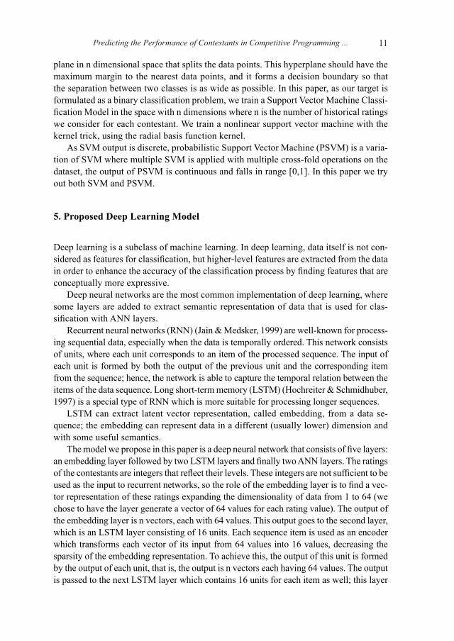
5. Proposed Deep Learning Model

Deep learning is a subclass of machine learning. In deep learning, data itself is not con-sidered as features for classification, but higher-level features are extracted from the data in order to enhance the accuracy of the classification process by finding features that are conceptually more expressive.

Deep neural networks are the most common implementation of deep learning, where some layers are added to extract semantic representation of data that is used for clas-sification with ANN layers.

Recurrent neural networks (RNN) (Jain & Medsker, 1999) are well-known for process-ing sequential data, especially when the data is temporally ordered. This network consists of units, where each unit corresponds to an item of the processed sequence. The input of each unit is formed by both the output of the previous unit and the corresponding item from the sequence; hence, the network is able to capture the temporal relation between the items of the data sequence. Long short-term memory (LSTM) (Hochreiter & Schmidhuber, 1997) is a special type of RNN which is more suitable for processing longer sequences.

LSTM can extract latent vector representation, called embedding, from a data se-quence; the embedding can represent data in a different (usually lower) dimension and with some useful semantics.

The model we propose in this paper is a deep neural network that consists of five layers: an embedding layer followed by two LSTM layers and finally two ANN layers. The ratings of the contestants are integers that reflect their levels. These integers are not sufficient to be used as the input to recurrent networks, so the role of the embedding layer is to find a vec-tor representation of these ratings expanding the dimensionality of data from 1 to 64 (we chose to have the layer generate a vector of 64 values for each rating value). The output of the embedding layer is n vectors, each with 64 values. This output goes to the second layer, which is an LSTM layer consisting of 16 units. Each sequence item is used as an encoder which transforms each vector of its input from 64 values into 16 values, decreasing the sparsity of the embedding representation. To achieve this, the output of this unit is formed by the output of each unit, that is, the output is n vectors each having 64 values. The output is passed to the next LSTM layer which contains 16 units for each item as well; this layer


generates a single vector representation of the ratings sequence, which is the output of the last unit of this network. This vector has 16 values. The vector representation is passed to a fully connected ANN network with 10 neurons, this layer is a classification layer whose activation function is ReLU. Its output is connected to a single neuron which constitutes the last layer of the network. This neuron has a Sigmoid activation function whose output is the probability that the input ratings sequence belongs to the positive class, that is, the contestant performance will decrease. Fig. 2 shows the network structure.

The network is trained by minimizing the cross-entropy loss function and the Adam optimizer is used to train the network.

6. Experiment and Results

To evaluate the proposed machine learning method along with the deep learning model, we conduct a real experiment. This section explains the data collection, the evaluation metrics and the detailed results.

Rating sequence

Embedding layer

LSTM layer

LSTM layer

Dense layer

Output dense layer

Input (n values)

n*64

n*16

16

10

Output: Single value, probability of positive class

Fig. 2. Structure of proposed deep learning model.


6.1. The Dataset

To get data about competitive programming contestants, we use the data available from the website CodeForces.* This website is widely used for training people in competitive programming, moreover, it provides a rating system that allows each member to have a rate, which reflects the level of this member and changes after each round of competition conducted by the website.

Codeforces provides a public application programming interface (API)**, this API allows access to public data from the website and its users. To collect our dataset, firstly we used the ‘user.ratedList’ API method to get a list of users who have participated in at least one rated contest, we are interested only in active users, so we got about 21,000 users. We could get the rating history of each user by using ‘user.rating’ API method, so we eliminated the users who had less than 20 ratings, leaving us with 6876 users.

We chose 10 as the length of rating sequence that can reflect the contestant perfor-mance. We generated the dataset items where each item input is a sequence of 10 ratings and the output is a binary number 0 or 1 calculated by the next 10 ratings using the func-tion T as described in section 3 of this paper.

Many items may be generated by a single user, as every 20 consecutive ratings of the user can generate an item, so we used a window with a width of 20 to pass over the con-testant ratings and generate the items. Eventually our dataset contained 233629 items.

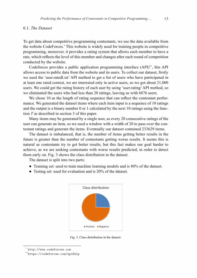
The dataset is imbalanced, that is, the number of items getting better results in the future is greater than the number of contestants getting worse results. It seems this is natural as contestants try to get better results, but this fact makes our goal harder to achieve, as we are seeking contestants with worse results predicted, in order to detect them early on. Fig. 3 shows the class distribution in the dataset.

The dataset is split into two parts:Training set: used to train machine learning models and is 80% of the dataset. ●Testing set: used for evaluation and is 20% of the dataset. ●

* http://www.codeforces.com** https://codeforces.com/apiHelp

Class distribution

Positive Negative

Fig. 3. Class distribution in the dataset.


6.2. Evaluation Metrics

To evaluate the different proposed models, we are going to use well-known evaluation metrics in classification tasks.

6.2.1. Area Under ROC Curve (AUROC)The receiver operating characteristics (ROC) curve is an important curve used to evaluate machine learning models. It represents the relation among sensitivity of the model with the specificity and the threshold used to choose the class. This curve reflects the perfor-mance of the model, so the area under this curve can reflect how perfect the model is.

6.2.2. Accuracy The accuracy of the model is the ratio of the items that are classified correctly:

]

𝑅𝐶(𝑅) = 1𝑛 2⁄ � 𝑟𝑖

𝑖=𝑛

𝑖=𝑛/2− 1𝑛 2⁄ � 𝑟𝑖

𝑛/2−1

𝑖=1

𝑇(𝑅) = �1, 𝑅𝐶(𝑅) < 00, 𝑅𝐶(𝑅) ≥ 0

𝑍(𝑅) = 𝛽0 + 𝛽1𝑟1 + 𝛽2𝑟2 + ⋯+ 𝛽𝑛𝑟𝑛

𝛽0,𝛽1,𝛽2, … ,𝛽𝑛

𝐿(𝑅) = 11 − 𝑒−𝑍(𝑅)

𝑐𝑙𝑎𝑠𝑠 = �0, 𝐿(𝑅) < 𝑡ℎ1, 𝐿(𝑅) ≥ 𝑡ℎ




𝑃(𝑦) = 1�2𝜋𝜎𝑦2


2

2𝜎𝑦2�

𝜃𝑦 = ( 𝜃𝑦1,𝜃𝑦2, … ., 𝜃𝑦𝑛)

𝜃𝑦𝑖

𝑃(𝑟|𝑦)




𝑎𝑐𝑐𝑢𝑟𝑎𝑐𝑦 = 𝑇𝑃 + 𝑇𝑁𝑁

Where TP is the number of positive items classified correctly, TN is the number of negative items classified correctly, and N is the number of all classified items.

6.2.3. Precision The precision of the model is the ratio of correct positive items:

𝑅𝐶(𝑅) = 1𝑛 2⁄ � 𝑟𝑖

𝑖=𝑛

𝑖=𝑛/2− 1𝑛 2⁄ � 𝑟𝑖

𝑛/2−1

𝑖=1

𝑇(𝑅) = �1, 𝑅𝐶(𝑅) < 00, 𝑅𝐶(𝑅) ≥ 0

𝑍(𝑅) = 𝛽0 + 𝛽1𝑟1 + 𝛽2𝑟2 + ⋯+ 𝛽𝑛𝑟𝑛

𝛽0,𝛽1,𝛽2, … ,𝛽𝑛

𝐿(𝑅) = 11 − 𝑒−𝑍(𝑅)

𝑐𝑙𝑎𝑠𝑠 = �0, 𝐿(𝑅) < 𝑡ℎ1, 𝐿(𝑅) ≥ 𝑡ℎ




𝑃(𝑦) = 1�2𝜋𝜎𝑦2


2

2𝜎𝑦2�

𝜃𝑦 = ( 𝜃𝑦1,𝜃𝑦2, … ., 𝜃𝑦𝑛)

𝜃𝑦𝑖

𝑃(𝑟|𝑦)





𝑃𝑟𝑒𝑐𝑖𝑠𝑖𝑜𝑛 = 𝑇𝑃𝑇𝑃 + 𝐹𝑃

Where FP is the items that are wrongly classified as positive when they are negative.

6.2.4. RecallThe recall is the ratio of positive items that are correctly classified as positive:

𝑅𝐶(𝑅) = 1𝑛 2⁄ � 𝑟𝑖

𝑖=𝑛

𝑖=𝑛/2− 1𝑛 2⁄ � 𝑟𝑖

𝑛/2−1

𝑖=1

𝑇(𝑅) = �1, 𝑅𝐶(𝑅) < 00, 𝑅𝐶(𝑅) ≥ 0

𝑍(𝑅) = 𝛽0 + 𝛽1𝑟1 + 𝛽2𝑟2 + ⋯+ 𝛽𝑛𝑟𝑛

𝛽0,𝛽1,𝛽2, … ,𝛽𝑛

𝐿(𝑅) = 11 − 𝑒−𝑍(𝑅)

𝑐𝑙𝑎𝑠𝑠 = �0, 𝐿(𝑅) < 𝑡ℎ1, 𝐿(𝑅) ≥ 𝑡ℎ




𝑃(𝑦) = 1�2𝜋𝜎𝑦2


2

2𝜎𝑦2�

𝜃𝑦 = ( 𝜃𝑦1,𝜃𝑦2, … ., 𝜃𝑦𝑛)

𝜃𝑦𝑖

𝑃(𝑟|𝑦)






𝑅𝑒𝑐𝑎𝑙𝑙 = 𝑇𝑃𝑇𝑃 + 𝐹𝑁

Where FN are positive items that are wrongly classified as negative. This metric is the

most important one in our study, because it is more important to detect most of the con-testants with performance decreasing rather than getting high classification precision.

6.2.5. F1 ScoreF1 score can merge both precision and recall; it is more suitable than accuracy when data is imbalanced:

𝑅𝐶(𝑅) = 1𝑛 2⁄ � 𝑟𝑖

𝑖=𝑛

𝑖=𝑛/2− 1𝑛 2⁄ � 𝑟𝑖

𝑛/2−1

𝑖=1

𝑇(𝑅) = �1, 𝑅𝐶(𝑅) < 00, 𝑅𝐶(𝑅) ≥ 0

𝑍(𝑅) = 𝛽0 + 𝛽1𝑟1 + 𝛽2𝑟2 + ⋯+ 𝛽𝑛𝑟𝑛

𝛽0,𝛽1,𝛽2, … ,𝛽𝑛

𝐿(𝑅) = 11 − 𝑒−𝑍(𝑅)

𝑐𝑙𝑎𝑠𝑠 = �0, 𝐿(𝑅) < 𝑡ℎ1, 𝐿(𝑅) ≥ 𝑡ℎ




𝑃(𝑦) = 1�2𝜋𝜎𝑦2


2

2𝜎𝑦2�

𝜃𝑦 = ( 𝜃𝑦1,𝜃𝑦2, … ., 𝜃𝑦𝑛)

𝜃𝑦𝑖

𝑃(𝑟|𝑦)







𝐹1 𝑠𝑐𝑜𝑟𝑒 = 2 ∗ 𝑃𝑟𝑒𝑐𝑖𝑠𝑖𝑜𝑛 ∗ 𝑟𝑒𝑐𝑎𝑙𝑙𝑃𝑟𝑒𝑐𝑖𝑠𝑖𝑜𝑛 + 𝑟𝑒𝑐𝑎𝑙𝑙


7. Results

The six models presented in this paper are trained using the training part of the dataset, then the testing set is used to evaluate the performance of these models.

To handle the data imbalance problem of the dataset, we use class weights during the training of the models, where each class is weighted so that the weights reflect the ratio of class in the training data:

𝑅𝐶(𝑅) = 1𝑛 2⁄ � 𝑟𝑖

𝑖=𝑛

𝑖=𝑛/2− 1𝑛 2⁄ � 𝑟𝑖

𝑛/2−1

𝑖=1

𝑇(𝑅) = �1, 𝑅𝐶(𝑅) < 00, 𝑅𝐶(𝑅) ≥ 0

𝑍(𝑅) = 𝛽0 + 𝛽1𝑟1 + 𝛽2𝑟2 + ⋯+ 𝛽𝑛𝑟𝑛

𝛽0,𝛽1,𝛽2, … ,𝛽𝑛

𝐿(𝑅) = 11 − 𝑒−𝑍(𝑅)

𝑐𝑙𝑎𝑠𝑠 = �0, 𝐿(𝑅) < 𝑡ℎ1, 𝐿(𝑅) ≥ 𝑡ℎ




𝑃(𝑦) = 1�2𝜋𝜎𝑦2


2

2𝜎𝑦2�

𝜃𝑦 = ( 𝜃𝑦1,𝜃𝑦2, … ., 𝜃𝑦𝑛)

𝜃𝑦𝑖

𝑃(𝑟|𝑦)







𝐹1 𝑠𝑐𝑜𝑟𝑒 = 2 ∗ 𝑃𝑟𝑒𝑐𝑖𝑠𝑖𝑜𝑛 ∗ 𝑟𝑒𝑐𝑎𝑙𝑙𝑃𝑟𝑒𝑐𝑖𝑠𝑖𝑜𝑛 + 𝑟𝑒𝑐𝑎𝑙𝑙

𝑊𝑐 = 𝑁2 ∗ 𝑁𝑐

Where Wc is the weight for class c, N is the total number of items in the dataset and

Nc is the number of items with class c in the dataset.Fig. 4 shows the AUROC of the models:

Linear regression (LR). ●Random forest (RF). ●Artificial neural network (ANN). ●Multinomial Naïve Bayes (MNB). ●Gaussian Naïve Bayes (GNB). ●Probabilistic Support vector machine (PSVM). ●Deep learning model (DL). ●

Note that this measure cannot be calculated for support vector machines as their out-put is discrete, unlike other models where the output is a probabilistic continuous value that falls in range (0,1).

We can notice that the deep learning model achieved the best value for this metric. MLP and RF achieved good results as well, whereas probabilistic models had poor per-formance.

Class distribution

Positive Negative

Class distribution

Positive Negative

0,53306943 0,638623737 0,672690034 0,679866965 0,720696435 0,733851101

0,899119249

00,10,20,30,40,50,60,70,80,9

1

GNB MNB LR PSVM RF MLP DL

AUROC

AUROC

Fig. 4. AUROC of different models.


Fig. 5 shows the accuracy of different models: deep learning achieved the best result for this metric, and the support vector machine had good accuracy as well, whereas lin-ear regression had the poorest result.

Fig. 6 shows the precision of different models: linear regression outperformed all other models including the deep learning one. However, this metric does not reflect the overall performance of the model, because it is more important to detect most con-testants with poor predicted performance rather than getting a high ratio of correctly detected contestants.

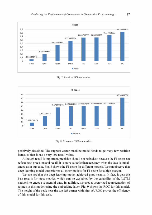
Fig. 7 shows the recall metric of the different models: the deep learning model has the highest recall while the random forest model also achieved good results. Recall is very important as it refers to the ratio of contestants with poor performance that are

Class distribution

Positive Negative

Class distribution

Positive Negative

0,53306943 0,638623737 0,672690034 0,679866965 0,720696435 0,733851101

0,899119249

00,10,20,30,40,50,60,70,80,9

1

GNB MNB LR PSVM RF MLP DL

AUROC

AUROC

0,408787399 0,497410435

0,669434576 0,674485297 0,674990371 0,696657107 0,754697599

0,837242649

00,10,20,30,40,50,60,70,80,9

LR RF MNB MLP PSVM GNB SVM DL

Accuracy

Accuracy

Fig. 5. Accuracy of different models.

Class distribution

Positive Negative

Class distribution

Positive Negative

0,408787399 0,497410435

0,669434576 0,674485297 0,674990371 0,696657107 0,754697599

0,837242649

00,10,20,30,40,50,60,70,80,9


Accuracy

Accuracy

0,34092219 0,37759229 0,399142128 0,411353803 0,417046228

0,564546784 0,636617704

0,755522828

0

0,1

0,2

0,3

0,4

0,5

0,6

0,7

0,8

RF GNB MNB SVM MLP PSVM DL LR

Precision

Precision

Fig. 6. Precision of different models.


positively classified. The support vector machine model tends to get very few positive items, so that it has a very low recall value.

Although recall is important, precision should not be bad, so because the F1 score can reflect both precision and recall, it is more suitable than accuracy when the data is imbal-anced as in our case. Fig. 8 shows the F1 score for different models. We can observe that deep learning model outperforms all other models for F1 score for a high margin.

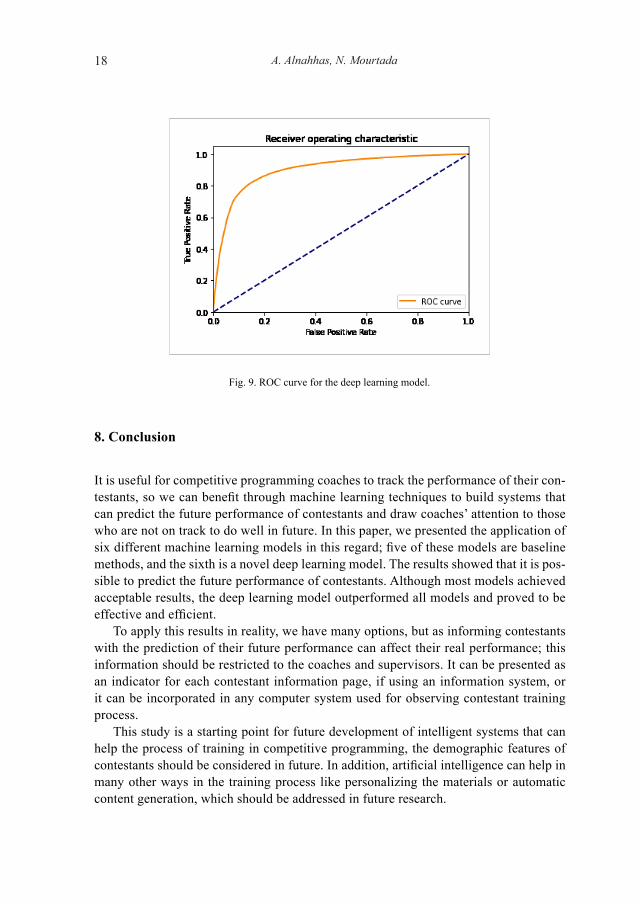
We can see that the deep learning model achieved good results. In fact, it gets the best results for most metrics, which can be explained by the capability of the LSTM network to encode sequential data. In addition, we used a vectorized representation of ratings in this model using the embedding layer. Fig. 9 shows the ROC for this model. The height of the peak near the top left corner with high AUROC proves the efficiency of this model for this task.

Class distribution

Positive Negative

Class distribution

Positive Negative

0,408787399 0,497410435

0,669434576 0,674485297 0,674990371 0,696657107 0,754697599

0,837242649

00,10,20,30,40,50,60,70,80,9


Accuracy

Accuracy

0,043441443

0,197726893

0,455499853

0,575463814 0,665719539 0,668219155

0,733411332 0,829452113

00,10,20,30,40,50,60,70,80,9

SVM GNB PSVM MNB LR MLP RF DL

Recall

Recall

Fig. 7. Recall of different models.

Class distribution

Positive Negative

Class distribution

Positive Negative

0,408787399 0,497410435

0,669434576 0,674485297 0,674990371 0,696657107 0,754697599

0,837242649

00,10,20,30,40,50,60,70,80,9


Accuracy

Accuracy

0,082158873

0,250290913

0,471353275 0,498523063 0,504194549 0,509228188 0,512827116

0,720353006

0

0,1

0,2

0,3

0,4

0,5

0,6

0,7

0,8

SVM GNB MNB RF PSVM MLP LR DL

F1 score

F1 score

Fig. 8. F1 score of different models.


8. Conclusion

It is useful for competitive programming coaches to track the performance of their con-testants, so we can benefit through machine learning techniques to build systems that can predict the future performance of contestants and draw coaches’ attention to those who are not on track to do well in future. In this paper, we presented the application of six different machine learning models in this regard; five of these models are baseline methods, and the sixth is a novel deep learning model. The results showed that it is pos-sible to predict the future performance of contestants. Although most models achieved acceptable results, the deep learning model outperformed all models and proved to be effective and efficient.

To apply this results in reality, we have many options, but as informing contestants with the prediction of their future performance can affect their real performance; this information should be restricted to the coaches and supervisors. It can be presented as an indicator for each contestant information page, if using an information system, or it can be incorporated in any computer system used for observing contestant training process.

This study is a starting point for future development of intelligent systems that can help the process of training in competitive programming, the demographic features of contestants should be considered in future. In addition, artificial intelligence can help in many other ways in the training process like personalizing the materials or automatic content generation, which should be addressed in future research.

Fig. 9. ROC curve for the deep learning model.


References

Al-Shabandar, R., Hussain, A., Laws, A., Keight, R., Lunn, J., & Radi, N. (2017). Machine learning approaches to predict learning outcomes in Massive open online courses. Paper presented at the 2017 International Joint Conference on Neural Networks (IJCNN).

Amra, I. A. A., & Maghari, A. Y. (2017). Students performance prediction using KNN and Naïve Bayesian. Paper presented at the 2017 8th International Conference on Information Technology (ICIT).

Babić, I. Đ. (2017). Machine learning methods in predicting the student academic motivation. Croatian Opera-tional Research Review, 443–461.

Colchester, K., Hagras, H., Alghazzawi, D., & Aldabbagh, G. (2017). A survey of artificial intelligence tech-niques employed for adaptive educational systems within e-learning platforms. Journal of Artificial Intel-ligence and Soft Computing Research, 7(1), 47–64.

Combéfis, S., & Paques, A. (2015). Organising national olympiads in informatics: A review of selection pro-cesses, trainings and promotion activities. Olympiads in Informatics, 9.

Hochreiter, S., & Schmidhuber, J. (1997). Long short-term memory. Neural Computation, 9(8), 1735–1780. Hussain, S., Muhsion, Z. F., Salal, Y. K., Theodoru, P., KurtoÄ lu, F., & Hazarika, G. (2019). Prediction model

on student performance based on internal assessment using deep learning. International Journal of Emerg-ing Technologies in Learning (iJET), 14(08), 4–22.

Jain, L. C., & Medsker, L. R. (1999). Recurrent Neural Networks: Design and Applications: CRC Press, Inc.Kingma, D. P., & Ba, J. (2014). Adam: A method for stochastic optimization. arXiv preprint arXiv:1412.6980. Kotsiantis, S., Pierrakeas, C., & Pintelas, P. (2004). Predicting students’ performance in distance learning using

machine learning techniques. Applied Artificial Intelligence, 18(5), 411–426. Koutina, M., & Kermanidis, K. L. (2011). Predicting postgraduate students’ performance using machine learn-

ing techniques Artificial intelligence applications and innovations (pp. 159–168): Springer.Liaw, A., & Wiener, M. (2002). Classification and regression by randomForest. R news, 2(3), 18–22. Ofori, F., Maina, E., & Gitonga, R. (2020). Using machine learning algorithms to predict students’ performance

and improve learning outcome: A literature based review. Journal of Information and Technology, 4(1), 33–55.

Quinlan, J. R. (1986). Induction of decision trees. Machine Learning, 1(1), 81–106. Sekeroglu, B., Dimililer, K., & Tuncal, K. (2019). Student performance prediction and classification using ma-

chine learning algorithms. Paper presented at the Proceedings of the 2019 8th International Conference on Educational and Information Technology.

Tan, M., & Shao, P. (2015). Prediction of student dropout in e-learning program through the use of machine learning method. International Journal of Emerging Technologies in Learning, 10(1).

Tanner, T., & Toivonen, H. (2010). Predicting and preventing student failure-using the k-nearest neighbour method to predict student performance in an online course environment. International Journal of Learning Technology, 5(4), 356.

Thai-Nghe, N., Drumond, L., Krohn-Grimberghe, A., & Schmidt-Thieme, L. (2010). Recommender system for predicting student performance. Procedia Computer Science, 1(2), 2811–2819.

Waheed, H., Hassan, S.-U., Aljohani, N. R., Hardman, J., Alelyani, S., & Nawaz, R. (2020). Predicting academ-ic performance of students from VLE big data using deep learning models. Computers in Human Behavior, 104, 106189.

Xu, J., Moon, K. H., & Van Der Schaar, M. (2017). A machine learning approach for tracking and predicting student performance in degree programs. IEEE Journal of Selected Topics in Signal Processing, 11(5), 742–753.


A. Alnahhas is a teacher at the faculty of information technology en-gineering, Damascus University, he holds a Ph.D. in artificial intel-ligence, he was involved in the training and preparation of national Olympiad in informatics since 2005, he was involved in many com-petitive programming activities, he has been the leader of Syrian del-egation to IOI for many years.

N. Mourtada is an information technology engineering student at the department of artificial intelligence, faculty of information technology engineering, Damascus University.

Predicting the Performance of Contestants in Competitive ...

Documents

Transcript of Predicting the Performance of Contestants in Competitive ...