Predicting stomatal responses to the environment from …€¦ · Original Article Predicting...

Original Article

Predicting stomatal responses to the environment from theoptimization of photosynthetic gain and hydraulic cost

John S. Sperry1, Martin D. Venturas1, William R. L. Anderegg1, Maurizio Mencuccini2,3, D. Scott Mackay4, YujieWang1 &David M. Love1

1Department of Biology, University of Utah, 257 S 1400E, Salt Lake City, UT 84112, USA, 2School of GeoSciences, University ofEdinburgh, West Mains Road, Edinburgh EH9 3Ju, UK, 3ICREA at CREAF, Cerdanyola del Vallès, Barcelona 08193, Spain and4Department of Geography, State University of New York, Buffalo, NY 14260, USA

ABSTRACT

Stomatal regulation presumably evolved to optimize CO2 forH2O exchange in response to changing conditions. If theoptimization criterion can be readily measured or calculated,then stomatal responses can be efficiently modelled without re-course to empirical models or underlying mechanism. Previousefforts have been challenged by the lack of a transparent indexfor the cost of losing water. Yet it is accepted that stomatacontrol water loss to avoid excessive loss of hydraulic conduc-tance from cavitation and soil drying. Proximity to hydraulicfailure and desiccation can represent the cost of water loss. Ifat any given instant, the stomatal aperture adjusts to maximizethe instantaneous difference between photosynthetic gain andhydraulic cost, then a model can predict the trajectory of sto-matal responses to changes in environment across time. Resultsof this optimization model are consistent with the widely usedBall–Berry–Leuning empirical model (r2> 0.99) across a widerange of vapour pressure deficits and ambient CO2 concentra-tions for wet soil. The advantage of the optimization approachis the absence of empirical coefficients, applicability to dry aswell as wet soil and prediction of plant hydraulic status alongwith gas exchange.

Key-words: Ball–Berry–Leuning model; Cowan–Farquhar op-timization; hydraulic limitations; photosynthetic optimization;plant drought responses; plant gas exchange; stomatal model-ling; stomatal regulation; xylem cavitation.

INTRODUCTION

Land plants face a fundamental carbon-for-water trade-off.They must open their stomata for photosynthetic gain, butdoing so promotes water loss. Plant responses to environmentrepresent a balancing act that presumably optimizes thistrade-off in some manner (Cowan & Farquhar 1977; Katulet al. 2010; Manzoni et al. 2011; Medlyn et al. 2011; Bonanet al. 2014; Prentice et al. 2014). When air and soil are dry,photosynthesis is sacrificed in favour of reduced water loss(Schulze & Hall 1982). When ambient CO2 is scarce, greaterwater loss is tolerated in favour of photosynthesis (Morison

1987). The trade-off has seemingly resulted in tight coordina-tion between capacity to supply and transpire water (hydraulicconductance, k, and diffusive conductance to water vapour,Gw) and the maximum capacity for photosynthesis (carboxyla-tion rate,Vmax, and electron transport rate, Jmax; Brodribb et al.2002). If the fulcrum on which this trade-off balances could beidentified, it would greatly simplify the difficult problem ofpredicting how plant gas exchange responds to environmentalcues (Prentice et al. 2014). In this paper, we describe such abalancing point, explain how it can be readily quantified frommeasurable plant traits and processes, and evaluate theresulting patterns in stomatal regulation of gas exchange andxylem pressure.

The utility of a stomatal optimization framework has longbeen recognized, but uncertainty in the optimization criteriaand its relation to true fitness costs and benefits has limited itspotential for understanding and modelling stomatal behaviour,particularly in response to drying soil. A long-standing theory(Cowan & Farquhar 1977) assumes stomatal regulationmaximizes cumulative photosynthesis (A) for a fixed amountof water transpired (cumulative E) over a time period. This isa ‘constrained-optimization’ problem (total E is constrained)whose solution specifies a constant Lagrangian multiplier, λ′,which equals a constant ∂E/∂A. Stomata are assumed tomaintain ∂E/∂A= λ′ at every instant throughout the time pe-riod, and this behaviour can be modelled (Cowan & Farquhar1977; Cowan 1982; Makala et al. 1996; Medlyn et al. 2011;Manzoni et al. 2013). But a persistent problem is in puttingan a priori number on λ′. Which of the infinite values for∂E/∂A is the right one? The ∂E/∂A is assumed to representthe ‘unit marginal cost’ (∂cost/∂gain) where the cost of stoma-tal opening is equated with E and A is the gain (Cowan 1982;p. 591). But it has been challenging to specify the optimal mar-ginal cost, and how it might vary with species, environmentand time (Givnish 1986; Manzoni et al. 2011; Manzoni et al.2013; Buckley et al. 2016).

A related issue is whether the optimization problem is prop-erly framed (Wolf et al. 2016). Instead of maximizing photosyn-thesis for an arbitrarily fixed amount of water loss over someperiod of time, is it not more to the point that plants wouldmaintain the greatest carbon gain relative to the actual cost ofwater loss at all times, regardless of the amount of water usedor time period involved? Such plants will use more water whenCorrespondence: J. S. Sperry. e-mail: [email protected]

© 2016 John Wiley & Sons Ltd 1

doi: 10.1111/pce.12852Plant, Cell and Environment (2016)

it is cheap and there is opportunity for more photosyntheticgain, and they will use less water when its cost rises or thereis less photosynthetic opportunity. In this ‘profit maximization’optimization, there is no arbitrary constraint on the amount ofwater the plant can use over time, and there is no constantLagrangian multiplier involved in its solution (no λ′). Theequation is: profit = gain� cost. Maximum profit is found bysetting the derivative of this equation to zero, at which point∂cost/∂gain= 1. In profit maximization, the unit marginal costshould always equal 1. But to implement this scheme, the costof water use must be specified.

After the leaf scale concept of coupled carbon and watereconomy arose we have learned how xylem cavitation limitsthe transpiration stream (Tyree & Sperry 1988; Sperry et al.1998; Sperry & Love 2015). As the physiological importanceof cavitation became accepted, a second perspective on stoma-tal regulation emerged, which is that stomata act to maximizephotosynthesis under the constraint of avoiding excessivexylem cavitation (Feild & Holbrook 1989; Sparks & Black1999; Tombesi et al. 2015; Novick et al. 2016). It is possible tomodel stomatal behaviour in response to water stress solelyon the principle that stomata close in proportion to the threatof cavitation on canopy water supply (Sperry & Love 2015;Sperry et al. 2016). While this hydraulic approach may provepractical in many applications, it ignores the role of stomatain regulating and responding to photosynthesis, and it doesnot emerge explicitly from the carbon-for-water tradeoff. How-ever, it does identify the loss of conductivity to cavitation as animportant fitness cost ofmoving water.Mortality is the ultimatefitness cost, and it exhibits a strong linkage to vascular dysfunc-tion (Kukowski et al. 2013; McDowell et al. 2013; Anderegget al. 2015; Anderegg et al. 2016).

Perhaps, the hydraulic models are providing a proxy for thecost of water loss, thus allowing the implementation of theprofit maximization theory. Hydraulics provide a ‘cost’ functionfor stomatal opening, and the corresponding photosynthetic‘gain’ function can be obtained from trait- and process-basedmodels of photosynthesis. The stomatal regulation that maxi-mizes the profit (where ∂cost/∂gain= 1) can bemodelled on thisbasis. In this paper, we develop this perspective and explore itspotential for improving our understanding and ability to modelstomatal responses to environmental forcing. Its predictionsare compared to those of a purely hydraulic model for stomatalconductance (Sperry & Love 2015; Sperry et al. 2016) and to awidely used empirical model (Ball, Berry, Leuning [BBL];Leuning 1995). The contrast in stomatal behaviour betweenprofit maximization versus the ∂E/∂A= λ′ constrained optimi-zation is discussed.

Stomatal response modelling does need improvement. Wecan model leaf energy balance, photosynthesis, hydraulic con-ductance and transpiration reasonably well under any environ-mental situation if the diffusive conductance of the leaf (Gw) isknown (Collatz et al. 1991; Collatz et al. 1992). In lieu of a traitand process-based predictive model for stomatal control ofGw,models have relied on empirical relationships. Conventionalformulations employed by land-surface models assume anempirical model for the Gw response to atmospheric vapourpressure deficit (D), photosynthetic rate (A) and ambient

CO2 concentration (Ca) under wet soil conditions (e.g. theBBL model; Leuning 1995). The wet soil model is scaled witha second empirical model to yield theGw response to soil waterpotential (Ps; Powell et al. 2013). Besides the unsatisfying needto rely on empirical coefficients of unknown physiologicalmeaning, these coefficients must be either robust to widely dif-ferent plant and soil types or else known for relevant functionaltypes. The stomatal response to drying soil is especially chal-lenging (Williams et al. 1996; Darmour et al. 2010; Manzoniet al. 2011; Manzoni et al. 2013; Powell et al. 2013). Hence, thesearch continues for a better way to model stomatal responsesthat is grounded in relevant process and measurable traits.

THE MODEL

The hydraulic cost function

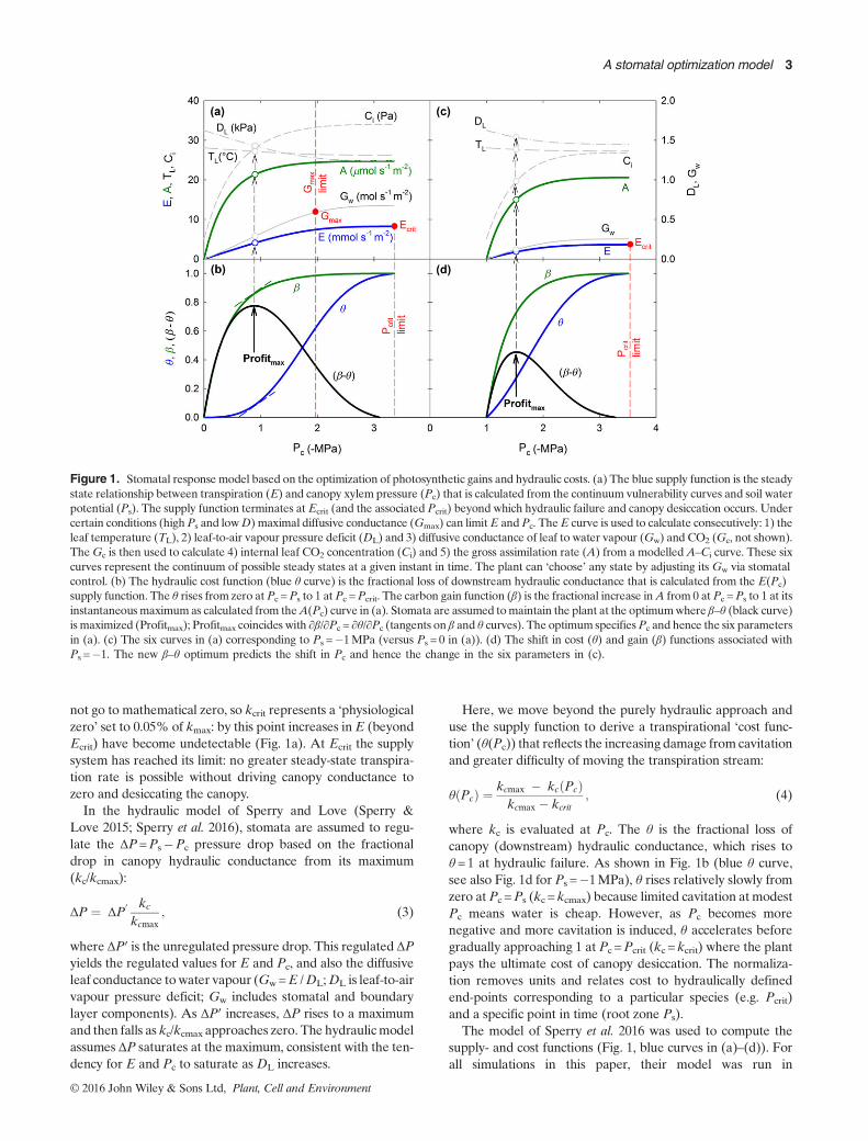
The hydraulic cost function is based on a ‘supply function’which describes the theoretical steady-state relation betweenE and canopy xylem pressure (Pc) at a given root zone soilwater potential, Ps (Fig. 1a blue E curve for Ps = 0; Fig. 1c bluecurve for Ps =�1MPa). Supply functions are calculated fromsoil and xylem vulnerability curves that describe how hydraulicconductance (k) of a soil or plant component declines from itsmaximum (kmax) in response to negative water pressure (P):

k ¼ kmax f Pð Þ: (1a)

For the plant, a two-parameter Weibull function for f(P)describes a wide range of vulnerability curves (Neufeldet al. 1992):

f Pð Þ ¼ e� �P=bð Þcð Þ; (1b)

analogous to the van Genuchten function used for in soil(van Genuchten 1980). The Weibull ‘b’ parameter is P atk/kmax = 0.37, and c controls whether the curve is a thresholdsigmoidal form (c> 1) or non-threshold ‘exponential’ curve(c near 1). Transpiration (E) induces a pressure drop(upstream P� downstream P=Pup�Pdown) across each soiland xylem element. At steady-state, E is the integral of eachelement’s vulnerability curve from Pup to Pdown (Sperry &Love 2015):

E ¼ ∫Pdown

Pupkmax f Pð Þ dP: (2)

By integrating across all vulnerability curves in the soil–plantsystem, the relation between E and a given total Ps�Pc pres-sure drop can be found. This ‘supply function’ starts at E=0at Pc =Ps, and rises to E=Ecrit at Pc =Pcrit (Fig. 1a, blue Ecurve, expressed per leaf area). It is a curve of increasing dam-age and risk. The curve is steepest and nearly linear at firstwhen pressures are modest and cavitation is minimal. It beginsto flatten as cavitation reduces hydraulic conductance andmore pressure drop is required to move water. The instanta-neous slope of the supply function at Pc is proportional to thehydraulic conductance in the canopy (kc∝ ∂E/∂Pc; Sperryet al. 2016). The kc declines from a maximum at E=0 (kcmax)to near 0 (kcrit) at E=Ecrit (Fig. 1a, end of blue E curve). Thef(P) functions (Eqn 1b and soil van Genuchten curves) do

2 J. S. Sperry et al.

© 2016 John Wiley & Sons Ltd, Plant, Cell and Environment

not go to mathematical zero, so kcrit represents a ‘physiologicalzero’ set to 0.05% of kmax: by this point increases inE (beyondEcrit) have become undetectable (Fig. 1a). At Ecrit the supplysystem has reached its limit: no greater steady-state transpira-tion rate is possible without driving canopy conductance tozero and desiccating the canopy.In the hydraulic model of Sperry and Love (Sperry &

Love 2015; Sperry et al. 2016), stomata are assumed to regu-late the ΔP=Ps�Pc pressure drop based on the fractionaldrop in canopy hydraulic conductance from its maximum(kc/kcmax):

ΔP ¼ ΔP′ kckcmax

; (3)

where ΔP′ is the unregulated pressure drop. This regulated ΔPyields the regulated values for E and Pc, and also the diffusiveleaf conductance towater vapour (Gw=E /DL;DL is leaf-to-airvapour pressure deficit; Gw includes stomatal and boundarylayer components). As ΔP′ increases, ΔP rises to a maximumand then falls as kc/kcmax approaches zero. The hydraulicmodelassumes ΔP saturates at the maximum, consistent with the ten-dency for E and Pc to saturate as DL increases.

Here, we move beyond the purely hydraulic approach anduse the supply function to derive a transpirational ‘cost func-tion’ (θ(Pc)) that reflects the increasing damage from cavitationand greater difficulty of moving the transpiration stream:

θ Pcð Þ ¼ kcmax � kc Pcð Þkcmax � kcrit

; (4)

where kc is evaluated at Pc. The θ is the fractional loss ofcanopy (downstream) hydraulic conductance, which rises toθ =1 at hydraulic failure. As shown in Fig. 1b (blue θ curve,see also Fig. 1d for Ps =�1MPa), θ rises relatively slowly fromzero at Pc =Ps (kc =kcmax) because limited cavitation at modestPc means water is cheap. However, as Pc becomes morenegative and more cavitation is induced, θ accelerates beforegradually approaching 1 at Pc =Pcrit (kc =kcrit) where the plantpays the ultimate cost of canopy desiccation. The normaliza-tion removes units and relates cost to hydraulically definedend-points corresponding to a particular species (e.g. Pcrit)and a specific point in time (root zone Ps).

The model of Sperry et al. 2016 was used to compute thesupply- and cost functions (Fig. 1, blue curves in (a)–(d)). Forall simulations in this paper, their model was run in

Figure 1. Stomatal response model based on the optimization of photosynthetic gains and hydraulic costs. (a) The blue supply function is the steadystate relationship between transpiration (E) and canopy xylem pressure (Pc) that is calculated from the continuum vulnerability curves and soil waterpotential (Ps). The supply function terminates at Ecrit (and the associated Pcrit) beyond which hydraulic failure and canopy desiccation occurs. Undercertain conditions (highPs and lowD) maximal diffusive conductance (Gmax) can limitE andPc. TheE curve is used to calculate consecutively: 1) theleaf temperature (TL), 2) leaf-to-air vapour pressure deficit (DL) and 3) diffusive conductance of leaf to water vapour (Gw) and CO2 (Gc, not shown).TheGc is then used to calculate 4) internal leaf CO2 concentration (Ci) and 5) the gross assimilation rate (A) from a modelledA–Ci curve. These sixcurves represent the continuum of possible steady states at a given instant in time. The plant can ‘choose’ any state by adjusting its Gw via stomatalcontrol. (b) The hydraulic cost function (blue θ curve) is the fractional loss of downstream hydraulic conductance that is calculated from the E(Pc)supply function. The θ rises from zero atPc =Ps to 1 at Pc =Pcrit. The carbon gain function (β) is the fractional increase inA from 0 at Pc =Ps to 1 at itsinstantaneousmaximumas calculated from theA(Pc) curve in (a). Stomata are assumed tomaintain the plant at the optimumwhere β–θ (black curve)is maximized (Profitmax); Profitmax coincides with ∂β/∂Pc = ∂θ/∂Pc (tangents on β and θ curves). The optimum specifiesPc and hence the six parametersin (a). (c) The six curves in (a) corresponding to Ps =�1MPa (versus Ps = 0 in (a)). (d) The shift in cost (θ) and gain (β) functions associated withPs =�1. The new β–θ optimum predicts the shift in Pc and hence the change in the six parameters in (c).

A stomatal optimization model 3


unsegmented mode (all xylem components assigned the sameWeibull f(P) function), with the xylem being limiting (rhizo-sphere average resistance of 5%). Themodel runs in reversibleand irreversible cavitation modes, but for the present purposereversibility was moot because all simulations were run fromlow to high water stress. The Sperry et al. model was revised

to express conductances on a leaf area basis to allow energybalance and photosynthesis calculations (‘big-leaf’ canopycomposed of identical leaves). The revised model is a VisualBasic for Applications macro in Microsoft Excel (code avail-able from the senior author). Hydraulic parameters underlyingthe supply function are listed in Table 1.

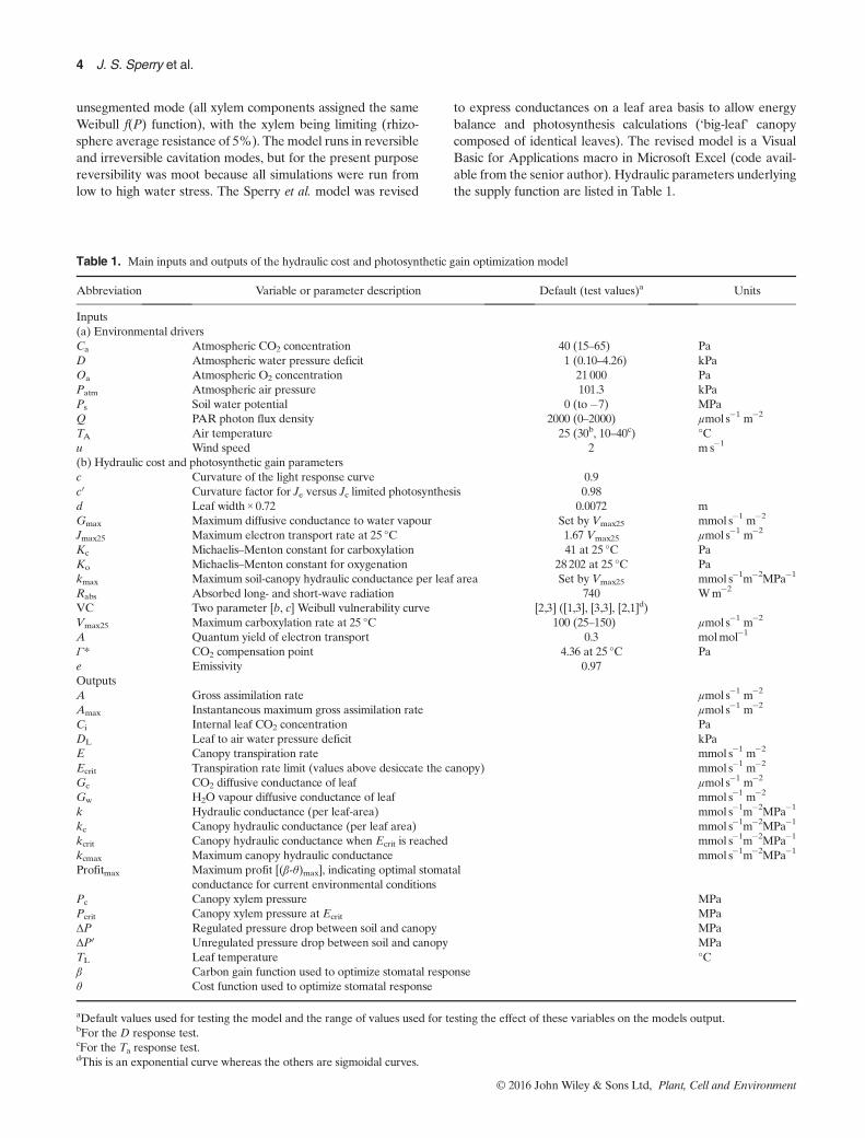
Table 1. Main inputs and outputs of the hydraulic cost and photosynthetic gain optimization model

Abbreviation Variable or parameter description Default (test values)a Units

Inputs(a) Environmental driversCa Atmospheric CO2 concentration 40 (15–65) PaD Atmospheric water pressure deficit 1 (0.10–4.26) kPaOa Atmospheric O2 concentration 21 000 PaPatm Atmospheric air pressure 101.3 kPaPs Soil water potential 0 (to�7) MPaQ PAR photon flux density 2000 (0–2000) μmol s�1 m�2

TA Air temperature 25 (30b, 10–40c) °Cu Wind speed 2 m s�1

(b) Hydraulic cost and photosynthetic gain parametersc Curvature of the light response curve 0.9c′ Curvature factor for Je versus Jc limited photosynthesis 0.98d Leaf width × 0.72 0.0072 mGmax Maximum diffusive conductance to water vapour Set by Vmax25 mmol s�1 m�2

Jmax25 Maximum electron transport rate at 25 °C 1.67 Vmax25 μmol s�1 m�2

Kc Michaelis–Menton constant for carboxylation 41 at 25 °C PaKo Michaelis–Menton constant for oxygenation 28 202 at 25 °C Pakmax Maximum soil-canopy hydraulic conductance per leaf area Set by Vmax25 mmol s�1m�2MPa�1

Rabs Absorbed long- and short-wave radiation 740 Wm�2

VC Two parameter [b, c] Weibull vulnerability curve [2,3] ([1,3], [3,3], [2,1]d)Vmax25 Maximum carboxylation rate at 25 °C 100 (25–150) μmol s�1 m�2

A Quantum yield of electron transport 0.3 molmol�1

Γ* CO2 compensation point 4.36 at 25 °C Pae Emissivity 0.97OutputsA Gross assimilation rate μmol s�1 m�2

Amax Instantaneous maximum gross assimilation rate μmol s�1 m�2

Ci Internal leaf CO2 concentration PaDL Leaf to air water pressure deficit kPaE Canopy transpiration rate mmol s�1 m�2

Ecrit Transpiration rate limit (values above desiccate the canopy) mmol s�1 m�2

Gc CO2 diffusive conductance of leaf μmol s�1 m�2

Gw H2O vapour diffusive conductance of leaf mmol s�1 m�2

k Hydraulic conductance (per leaf-area) mmol s�1m�2MPa�1

kc Canopy hydraulic conductance (per leaf area) mmol s�1m�2MPa�1

kcrit Canopy hydraulic conductance when Ecrit is reached mmol s�1m�2MPa�1

kcmax Maximum canopy hydraulic conductance mmol s�1m�2MPa�1

Profitmax Maximum profit [(β-θ)max], indicating optimal stomatalconductance for current environmental conditions

Pc Canopy xylem pressure MPaPcrit Canopy xylem pressure at Ecrit MPaΔP Regulated pressure drop between soil and canopy MPaΔP′ Unregulated pressure drop between soil and canopy MPaTL Leaf temperature °Cβ Carbon gain function used to optimize stomatal responseθ Cost function used to optimize stomatal response

aDefault values used for testing the model and the range of values used for testing the effect of these variables on the models output.bFor the D response test.cFor the Ta response test.dThis is an exponential curve whereas the others are sigmoidal curves.



The photosynthetic gain function

The water supply function was translated into its correspond-ing carbon gain function. Figure 1a,b illustrates the step-wiseprocess for the indicated supply function for Psoil = 0,D=1kPa and Ta = 25 °C. In a nutshell, E from the supplyfunction is used to compute leaf temperature (TL) and DL

from energy balance (Fig. 1a, grey dashed TL and dash-dotted DL curves). The diffusive conductances of the leaf towater vapour and CO2 (Gw, Gc, respectively) are obtainedfrom E and DL (Fig. 1a, solid grey Gw curve). The gross as-similation rate, A, is then obtained from Gc and a modelledA–Ci curve (Fig. 1a, green A curve). A normalized gain func-tion (β(Pc)) is computed to complement the hydraulic costfunction (θ(Pc), Fig. 1b, green β curve). The gain functionis based on gross assimilation, without subtracting respira-tion, because in parallel with the cost function, its purposeis to represent the instantaneous gain of opening the stomata.The gross gain provides all energy needs, of which leaf respi-ration is just one.The leaf temperature, TL (°C), was calcu-lated for each supply-function E (E converted to two-sidedleaf area basis; Campbell & Norman 1998, Eqns 14.1, 14.3)using the linearized expression:

TL ¼ TA þ Rabs � εσTa4 � λE

Cp gr þ gHað Þ ; (5)

where Rabs is absorbed long- and short-wave radiation(Wm�2), ε is emissivity (0.97), σ is the Stefan–Boltzmanconstant (5.67 E� 8Wm�2 °K�4), Ta is mean air temperaturein °K (TA is in °C), λ is latent heat of vaporization (Jmol�1),Cp is specific heat capacity of dry air at constant pressure(29.3 Jmol�1 °C�1), gr and gHa are radiative and heatconductances (molm�2 s�1), respectively, for the leaf. ThegHa=0.189 (u/d)

�0.5, where u is mean windspeed (m s�1) abovethe leaf boundary layer, and d is set to 0.72∙leaf width in m.Temperature dependence of λ and gr were obtained fromCampbell & Norman (1998). Simulations used values inTable 1 unless noted. For constant TA, leaf temperature fallsfrom a maximum at E=0 as transpiration increases (Fig. 1a,grey dashed TL line).Leaf temperature was used to calculate Gw, by firstly

calculatingDL. The DL falls from a maximum at E=0 as tran-spiration lowers TL (Fig. 1a, grey dash-dotted DL line). TheGw=E/DL (Fig. 1a, grey solid Gw curve), and Gc =Gw / 1.6.The portion of the curves to the right of the vertical Gmax

dashed line in Fig. 1a,b corresponds to E above a limit set bya maximum Gw of the leaf (e.g. Gmax for maximal stomatalopening at the prevailing boundary layer conductance). TheGmax quickly becomes non-limiting as soil dries (e.g. Fig. 1c,dfor Ps =�1MPa) or D increases. Cuticular water loss wasassumed zero for present purposes of modelling Gw, becauseit only influences results at or beyond the point of completestomatal closure.With TL and Gc known, gross A was calculated from

established photosynthesis models. Rubisco-limited photosyn-thesis rate, Jc, was obtained from (e.g. Collatz et al. 1991;Medlyn et al. 2002):

Jc ¼ Vmax Ci � Γ�ð ÞCi þ Kc 1þ Oa

Ko

� � ; (6)

where Vmax is Rubisco’s maximum carboxylation rate(μmol s�1 m�2), Ci is internal CO2 concentration (Pa), Γ* isthe CO2 compensation point (Pa), Kc and Ko are Michaelis–Menten constants for carboxylation and oxygenation, respec-tively, and Oa is atmospheric O2 concentration (21000Pa; Kc,Ko, Γ* values from Bernacchi et al. 2001).

Electron transport-limited photosynthesis, Je (μmol s�1

m�2), was obtained from Medlyn et al. (2002):

Je ¼ J4� Ci � Γ �

Ci þ 2Γ � (7a)

J ¼αQ þ Jmax – αQ þ Jmaxð Þ2 � 4cαQJmax

� �0:5

2c; (7b)

where α is the quantum yield of electron transport (assumed at0.3mol photon mol�1 e), Q=PAR photon flux density(μmol s�1 m�2), J is the actual rate of electron transport(μmol s�1 m�2), Jmax is the maximum rate of electron transport(μmol s�1 m�2) and c defines the curvature of the light re-sponse curve (0.9).

The gross assimilation rate at a given Ci is the minimumvalue of Je and Jc. To obtain a smooth A versus Ci curve weused (Collatz et al. 1991):

A ¼Je þ Jc – Je þ Jcð Þ2 � 4c′JeJc

� �0:5

2c′; (8)

where c′ is a curvature factor (0.98).The temperature dependence of Ko, Kc and Γ* relative to

25 °C was modelled as in Bernacchi et al. (2001) and Medlynet al. (2002). The temperature dependence of Jmax and Vmax

relative to 25 °C (Jmax25 andVmax25, respectively) was modelledusing Leuning (2002) (his equation 1 with parameters from hisTable 2). We assumed Vmax25 and Jmax25 co-varied, usingJmax25 =Vmax25 ∙ 1.67 (Medlyn et al. 2002).

The only unknown variable in Eqn 8 is Ci. However, weknow Gc from the supply function, which gives a secondequation for A:

A ¼ Gc Ca � Cið ÞPatm

; (9)

whereCa is atmospheric CO2 concentration (40Pa) and Patm isatmospheric pressure (101.3 kPa).We set Eqns 9 and 8 equal toeach other and solved for Ci, thereby obtainingA. Both Ci andA rise steeply with Gw before approaching saturation (Fig. 1a,grey dashed Ci curve and green A curve for parameter valueslisted in Table 1).

A normalized photosynthetic gain function (β(Pc)) wascalculated as

β Pcð Þ ¼ A Pcð ÞAmax

; (10)

whereA is evaluated at Pc, and Amax is the instantaneousmax-imumA over the full Pc range from Pc =Ps to Pc =Pcrit (not the



biochemical Amax). The gain function rises steeply from β =0 atPc =Ps as stomata open before flattening to β =1 asPc becomesmore negative and photosynthesis saturates (Fig. 1b, green βcurve). Like the θ(Pc) cost function, the gain function is nor-malized by the extremes, making it dimensionless, and relevantonly to the moment in time for which it is computed.

It is important to know that the family of f(Pc) curves inFig. 1a,b [E(Pc), TL(Pc), DL(Pc), Gw(Pc), Ci(Pc), A(Pc),θ(Pc), β(Pc)] represent steady-state values at a fixed instantwhere root zone Ps, atmosphericD, air temperature (Ta), windspeed (u) and light level (Q) are frozen in time. The plant canonly occupy one stable point on this theoretical constellationof possibilities. At the next time step, gradual shifts in soiland air moisture, temperature, windspeed and light create anew set of possibilities, only one of which the leaf will ‘target’via its stomatal response (assuming stomata keep pace withtypically gradual changes). Figure 1c,d shows, for example,how these functions shift when Ps drops to�1MPa. If a simplerule that approximated the presumably adaptive stomatal re-sponse can be found, then it becomes possible to anticipatewhere the plant regulates itself on these gradually shiftingcurves, assuming approximately steady-state conditions.

Instantaneous profit maximization

Wolf et al. (2016) pose the optimization criterion that at eachinstant in time, the stomata regulate canopy gas exchange andpressure to achieve themaximum profit, which is themaximumdifference between the normalized photosynthetic gain andhydraulic cost functions:

Prof itmax ¼ β Pcð Þ � θ Pcð Þ½ �max: (11a)

The maximization is achieved when:

∂β∂Pc

¼ ∂θ∂Pc

: (11b)

Note that β and θ can be expressed as functions ofGw insteadof Pc because of the coupling evident in Fig. 1. Figure 1b showsthe β–θ curve and its maximum (black curve), which coincideswith equal gain and cost derivatives (Fig. 1b, green and bluetangent lines to their respective curves). Instantaneous profit

maximization assumes a ‘use it or lose it’ reality with regardsto available soil water. Any more conservative water use strat-egy would backfirewhen soil water is not safe from competitors(i.e. instantaneous optimizers), drainage or surface evapora-tion. Although modelling optimization avoids specifying mech-anism, β and θ are determined by leaf-level phenomena: A forβ, and ∂E/∂Pc for θ. Plants can sense their photosynthetic statusand water balance (Paul & Foyer 2001; Tombesi et al. 2015),and hence potentially how both change in response to activecontrol of Gw and E. The steady-state assumption representsthe sustainable baseline β and θ. This is most appropriate formiddle of day gas exchange, which is generally a good predictorof daily totals (e.g. von Allmen et al. 2015).

Because the gain function accelerates more quickly fromzero and reaches 1 sooner than the cost function (Fig. 1b, greenversus blue curves), their maximum difference occurs at aunique intermediate Pc (Fig. 1b, black β–θ curve), which yieldsthe corresponding solutions for actualE,Gw,A,Gc,Ci, TL, andDL at that instant (Fig. 1, dashed arrows from maximum toopen symbols on curves in (a)).

As environmental conditions shift, so does the optimum. Theinfluence of drier soil (Ps =�1MPa) is shown in Fig. 1c,d. Thecost and gain functions are reset to start from 0 at Pc =Ps andrise to 1, but they rise from a more negative Ps. The rise ofthe gain function is not materially altered (only via changes inTL) because we assumed no direct effect of Pc onA. However,the cost function rises more steeply because it is computedfrom the more curved part of the supply function where morecavitation is occurring. The rapidly rising cost results in asmaller optimal soil-canopy ΔP, and a lower optimal Gw. TheFig. 1 example was computed from a sigmoidal vulnerabilitycurve (b=2, c=3). As explored under ‘model performance’the shape of the vulnerability curve influences how Ps changesthe cost function shape, and hence how the optimal pressuredrop and Gw change with drying soil.

The optimal solution also depends on D, TA, Ca and light.These environmental variables influence the optimum bychanging the shape of the gain function, as discussed under‘model performance’. When conditions flatten the gain func-tion (e.g. highD, lowCa, high TA; Fig. 2a, dashed green curve),the optimum shifts to more negative Pc (dashed black curve)driving an increase in the optimal soil-canopy pressure drop

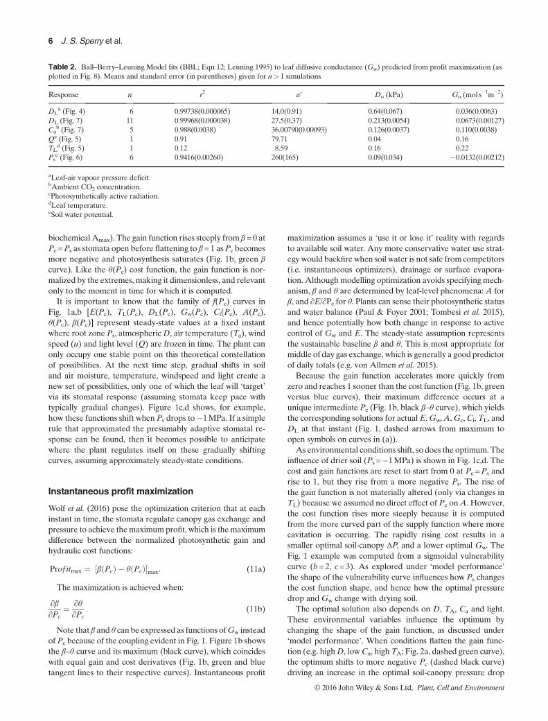
Table 2. Ball–Berry–Leuning Model fits (BBL; Eqn 12; Leuning 1995) to leaf diffusive conductance (Gw) predicted from profit maximization (asplotted in Fig. 8). Means and standard error (in parentheses) given for n> 1 simulations

Response n r2 a′ Do (kPa) Go (mol s�1m�2)

DLa (Fig. 4) 6 0.99738(0.000065) 14.0(0.91) 0.64(0.067) 0.036(0.0063)

DL (Fig. 7) 11 0.99968(0.000038) 27.5(0.37) 0.213(0.0054) 0.0673(0.00127)Ca

b (Fig. 7) 5 0.988(0.0038) 36.00790(0.00093) 0.126(0.0037) 0.110(0.0038)Qc (Fig. 5) 1 0.91 79.71 0.04 0.16TL

d (Fig. 5) 1 0.12 8.59 0.16 0.22Ps

e (Fig. 6) 6 0.9416(0.00260) 260(165) 0.09(0.034) �0.0132(0.00212)

aLeaf-air vapour pressure deficit.bAmbient CO2 concentration.cPhotosynthetically active radiation.dLeaf temperature.eSoil water potential.



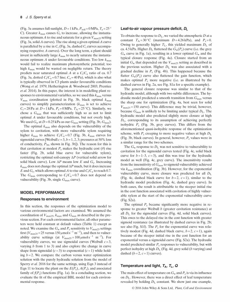
(Fig. 2a, red arrow, dashed vertical arrow). When conditionssteepen the gain function (e.g. low D, high Ca, low TA; Fig. 2asolid green curve), the optimum results in less negative Pc

(solid black curve) and a smaller soil-canopy pressure drop(Fig. 2a, solid vertical arrow).The key plant traits that influence the optimum include the

vulnerability curve (Weibull b, c parameters), the maximumsoil-canopy hydraulic conductance (kmax) and leaf diffusiveconductance (Gmax), and the photosynthetic capacity (Vmax25).More vulnerable xylem creates a faster rise in the cost functionand forces a less negative optimal Pc (Fig. 2b, solid curves forvulnerable xylem versus dashed for resistant). A higher kmax

andGmax increase E and Gw for a given optimal Pc. A greaterVmax25 creates a slower rise in the gain function and drivesoptimal Pc to a more negative value (Fig. 2a, dashed curves;see also Fig. S1d). As described next, the model predicts thatthese plant traits should be highly coordinated.

Longer-term optimization of photosynthetic andhydraulic parameters

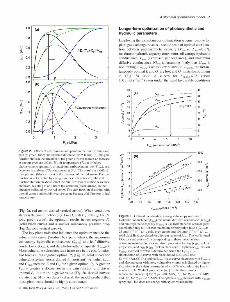
Employing the instantaneous optimization scheme to solve forplant gas exchange reveals a second scale of optimal coordina-tion between photosynthetic capacity (Vmax25 = Jmax25/1.67),maximum hydraulic capacity (maximum soil-canopy hydraulicconductance, kmax (expressed per leaf area), and maximumdiffusive conductance (Gmax). Assuming firstly that Gmax isnot limiting, if kmax is set too low relative to Vmax25, the instan-taneously optimalE andGc are low, andGc limits the optimumA (Fig. 3a, solid A curves for Vmax25 = 25 versus150μmol s�1m�2) even under the most favourable conditions

Figure 2. Effects of environment and plant on the cost (θ, blue) andgain (β, green) functions and their difference (β–θ, black). (a) The gainfunction shifts in the direction of the green arrow if there is an increasein vapour pressure deficit (D), air temperature (TA; at or belowphotosynthetic optimum), or maximum carboxylation rate (Vmax), or adecrease in ambient CO2 concentration (Ca). This results in a shift ofthe optimum (black arrows) in the direction of the red arrow. The costfunction is not affected by changes in these variables. (b) The costfunction shifts in the direction of the blue arrow as cavitation resistanceincreases, resulting in an shift of the optimum (black arrows) in thedirection indicated by the red arrow. The gain function also shifts withthe soil-canopy vulnerability curve change because of differences in leaftemperature.

Figure 3. Optimal coordination among soil-canopy maximumhydraulic conductance (kmax), maximum diffusive conductance (Gmax)and photosynthetic capacity (Vmax25). (a) Instantaneous optimal grossassimilation rate (A) for two maximum carboxylation rates (Vmax25):25μmol s�1 m�2 (A25, solid grey curve) and 150 μmol s�1 m�2 (A150,solid black line) calculated for different values of kmax. The leaf internalCO2 concentrations (Ci) corresponding to these instantaneousoptimum assimilation rates are also represented for A25 (Ci25, brokengrey curve) andA150 (Ci150, broken black curve). Optimal kmax for eachVmax25 (vertical arrows) is determined when the Ci/Ca = 0.7(intersection of Ci curves with black dotted Ci/Ca = 0.7 line;Ca = 40 kPa). (b) The optimal kmax (black curves) increases withVmax25,and also increases with more vulnerable xylem (as indicated by higherP50, which is the xylem pressure at which 50% of conductivity loss isreached). The Weibull parameters [b,c] for the three curvesrepresented were [1,3] for P50 =�0.88MPa, [2,3] for P50 =�1.77MPaand [3,3] for P50 =�2.70MPa. The optimalGmax increases with Vmax25

(grey line), but does not change with xylem vulnerability.



(Fig. 3a assumes full sunlight,D=1kPa, Psoil = 0MPa, Ta = 25 °C). Greater kmax causes Gc to increase, allowing the instanta-neous optimumA to rise and saturate for a givenVmax25 setting(Fig. 3a, solidA curves). The rise along a given optimalA curveis paralleled by a rise inCi (Fig. 3a, dashed Ci curves accompa-nying respective A curves). Over the long term, a plant shouldinvest in sufficiently large kmax to nearly saturate the instanta-neous optimum A under favourable conditions. Too low kmax

would fail to realize maximum photosynthetic potential; toohigh kmax would be wasted on negligible return. The theorypredicts near saturated optimal A at a Ci/Ca ratio of ca. 0.7(Fig. 3a, dotted Ci/Ca = 0.7 line; Ca = 40Pa), which is also whatis typically observed in C3 plants under favourable conditions(Wong et al. 1979; Hetherington & Woodward 2003; Prenticeet al. 2014). In this paper, the interest is in modelling plant re-sponses to environmental variables, so we used this kmax versusVmax coordination (plotted in Fig. 3b, black optimal kmax

curves) to simplify parameterization (kmax is set to achieveCi = 28Pa at D=1kPa, Ps = 0MPa, TA=25 °C). Similarly, wechose a Gmax that was sufficiently high so as not to limitoptimal A under favourable conditions, but not overly high.We usedGw atD=0.25 kPa as ourGmax setting (Fig. 3b,Gmax).

The optimal kmax also depends on the vulnerability of thexylem to cavitation, with more vulnerable xylem requiringhigher kmax to achieve Ci/Ca = 0.7 (Fig. 3b, kmax curves forsigmoidal curves [Weibull c=3, b=1, 2, 3; pressures at 50% lossof conductivity, P50, shown in Fig. 3b]). The reason for this isthat cavitation at modest Pc makes the hydraulic cost (θ) risefaster (Fig. 2b, solid blue curve for vulnerable xylem),restricting the optimal soil-canopy ΔP (vertical solid arrow forsolid black curve). Low ΔP means low E and Gc. Increasingkmax does not change the optimal ΔPmuch, but it does increaseE andGc, which allows optimalA to rise andCi/Ca to reach 0.7.The Gmax corresponding to Ci/Ca = 0.7 does not depend onvulnerability (Fig. 3b, single Gmax curve).

MODEL PERFORMANCE

Responses to environment

In this section, the responses of the optimization model tovarious environmental factors are examined. We assumed thecoordination of Vmax25, kmax andGmax as described in the pre-vious section. For each environmental factor, all other parame-ters were held constant at default values (Table 1) except asnoted. We examine theGw and Pc sensitivity to Vmax25 settingsfirst (Vmax25 = 25 versus 150μmol s�1 m�2), and then to vulner-ability curve settings (at Vmax25 = 100μmol s�1 m�2). Forvulnerability curves, we use sigmoidal curves (Weibull c=3,varying b from 1 to 3) and also explore the change in curveshape from sigmoidal (c=3) to exponential (c=1) while hold-ing b=2. We compare the carbon versus water optimizationsolution with the purely hydraulic solution from the model ofSperry et al. 2016 for the same settings, using Eqn 3 instead ofEqn 11 to locate the plant on the E(Pc), A(Pc), and associatedfamily of f(Pc) functions (Fig. 1a). In a concluding section, weevaluate the fit of the empirical BBL model for each environ-mental response.

Leaf-to-air vapour pressure deficit, DL

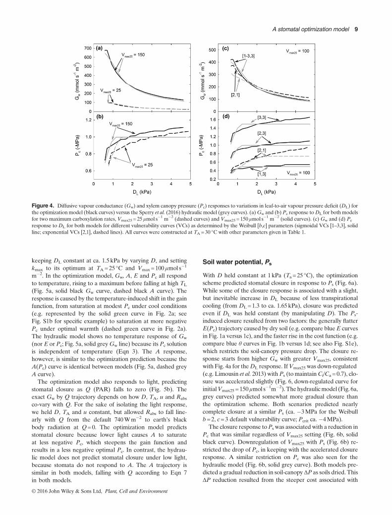
To obtain the response toDL, we varied the atmosphericD at aconstant TA=30 °C (maximum D=4.26kPa), and Ps = 0.Owing to generally higher TL, this yielded maximum DL ofca. 4.5kPa. HigherDL flattened theGw(Pc) curve (i.e. the greyGw curve in Fig. 1a), resulting in a lower optimal Gw and thetypical closure response (Fig. 4a). Closure started from aninitial Gw that depended on the Vmax25 setting as described inthe previous section. Higher DL was also associated with agradual decline in Pc (Fig. 4b). This happened because theflatter Gw(Pc) curve also flattened the gain function, whichmakes optimal Pc more negative (i.e. as illustrated by thedashed curves in Fig. 2a, see Fig. S1a for a specific example).

The general closure response was similar to that of thehydraulic model, although with two subtle differences. The hy-draulic model predicted a smooth transition from Gmax versusthe sharp one for optimization (Fig. 4a, best seen for solidVmax25 = 150 curve). This difference may be trivial, however,because Gmax is unlikely to be limiting under typical DL. Thehydraulic model also predicted slightly more closure at highDL, corresponding to its assumption of achieving perfectlyisohydric Pc (Fig. 3b, grey curves). This differs from theaforementioned quasi-isohydric response of the optimizationscheme, with Pc creeping to more negative values at high DL

(Fig. 3b, black curves). In general, however, Pc values were ina similar range for the two schemes.

The Gw response to DL was not sensitive to vulnerability tocavitation for the sigmoidal curves tested (Fig. 4c, solid blackcurve for b=1–3, c=3), and this was true for the hydraulicmodel as well (Fig. 4c, grey curve). The insensitivity resultsfrom the insensitivity ofGmax to sigmoid vulnerability achievedvia kmax coordination (Fig. 3b). However, for the exponentialvulnerability curve, more closure was predicted for all DL

(Fig. 4c, dashed black curve for b=2, c=1), similar to thehydraulic model prediction (Fig. 4c, dashed grey curve). Inboth cases, the result is attributable to the steeper initial risein the cost function associated with cavitation of highly vulner-able xylem at the start of the exponential vulnerability curve(Fig. S2a).

The optimal Pc became significantly more negative in re-sponse to greater Weibull b (greater cavitation resistance) atall DL for the sigmoidal curves (Fig. 4d, solid black curves).This owes to the delayed rise in the cost function with greatersigmoid resistance (as illustrated by dashed curves in Fig. 2b;see also Fig. S1f). The Pc for the exponential curve was rela-tively modest (Fig. 4d, dashed black curve, b=2, c=1), againbecause of the steeper initial rise in the cost function for anexponential versus a sigmoidal curve (Fig. S2a). The hydraulicmodel predicted similar Pc responses to vulnerability, but withperfect isohydry at highDL (Fig. 4d, grey solid (b varying) anddashed (b=2, c=1) curves).

Temperature and light, TA, TL, Q

Themain effect of temperature onGw andPc is via its influenceon DL. However, there was a direct effect of leaf temperaturerevealed by holding DL constant. We show just one example,



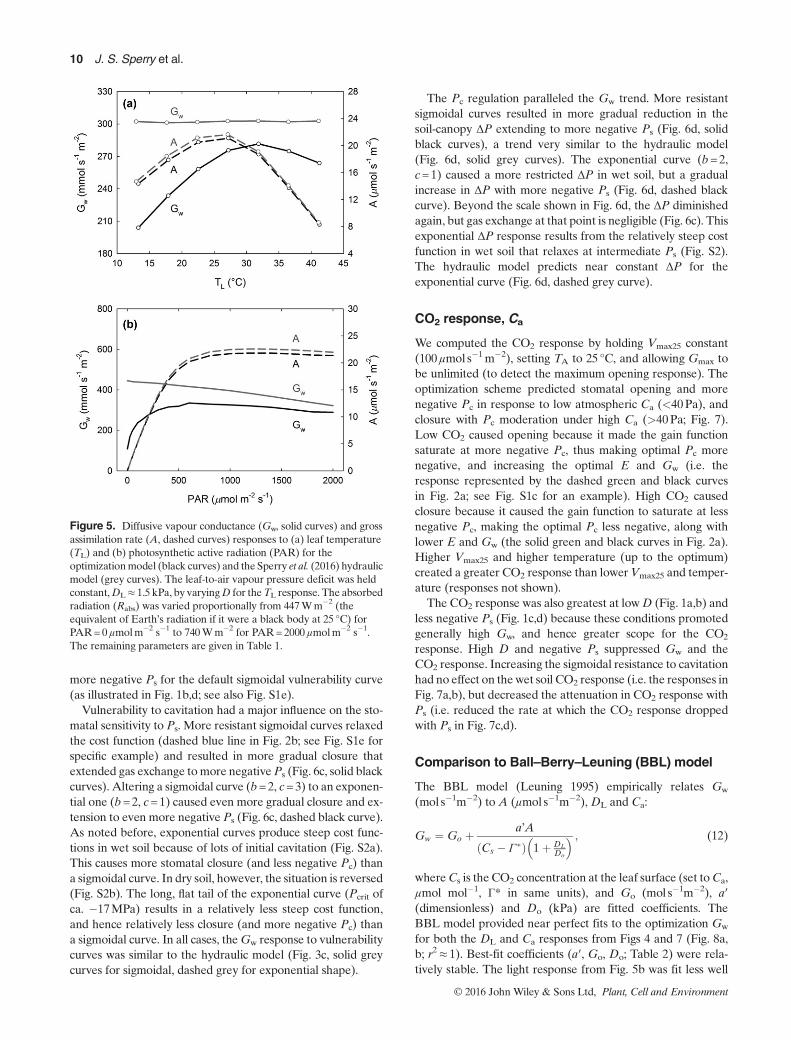
keeping DL constant at ca. 1.5kPa by varying D, and settingkmax to its optimum at TA=25 °C and Vmax =100μmol s�1

m�2. In the optimization model, Gw, A, E and Pc all respondto temperature, rising to a maximum before falling at high TL

(Fig. 5a, solid black Gw curve, dashed black A curve). Theresponse is caused by the temperature-induced shift in the gainfunction, from saturation at modest Pc under cool conditions(e.g. represented by the solid green curve in Fig. 2a; seeFig. S1b for specific example) to saturation at more negativePc under optimal warmth (dashed green curve in Fig. 2a).The hydraulic model shows no temperature response of Gw

(nor E or Pc; Fig. 5a, solid greyGw line) because its Pc solutionis independent of temperature (Eqn 3). The A response,however, is similar to the optimization prediction because theA(Pc) curve is identical between models (Fig. 5a, dashed greyA curve).The optimization model also responds to light, predicting

stomatal closure as Q (PAR) falls to zero (Fig. 5b). Theexact Gw by Q trajectory depends on how D, TA, u and Rabs

co-vary with Q. For the sake of isolating the light response,we held D, TA and u constant, but allowed Rabs to fall line-arly with Q from the default 740Wm�2 to earth’s blackbody radiation at Q=0. The optimization model predictsstomatal closure because lower light causes A to saturateat less negative Pc, which steepens the gain function andresults in a less negative optimal Pc. In contrast, the hydrau-lic model does not predict stomatal closure under low light,because stomata do not respond to A. The A trajectory issimilar in both models, falling with Q according to Eqn 7in both models.

Soil water potential, Ps

With D held constant at 1 kPa (Ta = 25 °C), the optimizationscheme predicted stomatal closure in response to Ps (Fig. 6a).While some of the closure response is associated with a slight,but inevitable increase in DL because of less transpirationalcooling (from DL=1.3 to ca. 1.65 kPa), closure was predictedeven if DL was held constant (by manipulating D). The Ps-induced closure resulted from two factors: the generally flatterE(Pc) trajectory caused by dry soil (e.g. compare blueE curvesin Fig. 1a versus 1c), and the faster rise in the cost function (e.g.compare blue θ curves in Fig. 1b versus 1d; see also Fig. S1e),which restricts the soil-canopy pressure drop. The closure re-sponse starts from higher Gw with greater Vmax25, consistentwith Fig. 4a for theDL response. IfVmax25 was down-regulated(e.g. Limousin et al. 2013) with Ps (to maintainCi/Ca = 0.7), clo-sure was accelerated slightly (Fig. 6, down-regulated curve forinitialVmax25 = 150μmol s�1m�2). Thehydraulicmodel (Fig. 6a,grey curves) predicted somewhat more gradual closure thanthe optimization scheme. Both scenarios predicted nearlycomplete closure at a similar Ps (ca. �3MPa for the Weibullb=2, c=3 default vulnerability curve; Pcrit ca. �4MPa).

The closure response toPs was associated with a reduction inPc that was similar regardless of Vmax25 setting (Fig. 6b, solidblack curve). Downregulation of Vmax25 with Ps (Fig. 6b) re-stricted the drop of Pc, in keeping with the accelerated closureresponse. A similar restriction on Pc was also seen for thehydraulic model (Fig. 6b, solid grey curve). Both models pre-dicted a gradual reduction in soil-canopy ΔP as soils dried. ThisΔP reduction resulted from the steeper cost associated with

Figure 4. Diffusive vapour conductance (Gw) and xylem canopy pressure (Pc) responses to variations in leaf-to-air vapour pressure deficit (DL) forthe optimizationmodel (black curves) versus the Sperry et al. (2016) hydraulic model (grey curves). (a)Gw and (b)Pc response toDL for both modelsfor two maximum carboxylation rates, Vmax25 = 25 μmol s�1 m�2 (dashed curves) and Vmax25 = 150μmol s�1 m�2 (solid curves). (c) Gw and (d) Pc

response toDL for both models for different vulnerability curves (VCs) as determined by the Weibull [b,c] parameters (sigmoidal VCs [1–3,3], solidline; exponential VCs [2,1], dashed lines). All curves were constructed at TA= 30 °C with other parameters given in Table 1.



more negative Ps for the default sigmoidal vulnerability curve(as illustrated in Fig. 1b,d; see also Fig. S1e).

Vulnerability to cavitation had a major influence on the sto-matal sensitivity to Ps. More resistant sigmoidal curves relaxedthe cost function (dashed blue line in Fig. 2b; see Fig. S1e forspecific example) and resulted in more gradual closure thatextended gas exchange tomore negativePs (Fig. 6c, solid blackcurves). Altering a sigmoidal curve (b=2, c=3) to an exponen-tial one (b=2, c=1) caused even more gradual closure and ex-tension to even more negative Ps (Fig. 6c, dashed black curve).As noted before, exponential curves produce steep cost func-tions in wet soil because of lots of initial cavitation (Fig. S2a).This causes more stomatal closure (and less negative Pc) thana sigmoidal curve. In dry soil, however, the situation is reversed(Fig. S2b). The long, flat tail of the exponential curve (Pcrit ofca. �17MPa) results in a relatively less steep cost function,and hence relatively less closure (and more negative Pc) thana sigmoidal curve. In all cases, theGw response to vulnerabilitycurves was similar to the hydraulic model (Fig. 3c, solid greycurves for sigmoidal, dashed grey for exponential shape).

The Pc regulation paralleled the Gw trend. More resistantsigmoidal curves resulted in more gradual reduction in thesoil-canopy ΔP extending to more negative Ps (Fig. 6d, solidblack curves), a trend very similar to the hydraulic model(Fig. 6d, solid grey curves). The exponential curve (b=2,c=1) caused a more restricted ΔP in wet soil, but a gradualincrease in ΔP with more negative Ps (Fig. 6d, dashed blackcurve). Beyond the scale shown in Fig. 6d, the ΔP diminishedagain, but gas exchange at that point is negligible (Fig. 6c). Thisexponential ΔP response results from the relatively steep costfunction in wet soil that relaxes at intermediate Ps (Fig. S2).The hydraulic model predicts near constant ΔP for theexponential curve (Fig. 6d, dashed grey curve).

CO2 response, Ca

We computed the CO2 response by holding Vmax25 constant(100μmol s�1m�2), setting TA to 25 °C, and allowing Gmax tobe unlimited (to detect the maximum opening response). Theoptimization scheme predicted stomatal opening and morenegative Pc in response to low atmospheric Ca (<40Pa), andclosure with Pc moderation under high Ca (>40Pa; Fig. 7).Low CO2 caused opening because it made the gain functionsaturate at more negative Pc, thus making optimal Pc morenegative, and increasing the optimal E and Gw (i.e. theresponse represented by the dashed green and black curvesin Fig. 2a; see Fig. S1c for an example). High CO2 causedclosure because it caused the gain function to saturate at lessnegative Pc, making the optimal Pc less negative, along withlower E and Gw (the solid green and black curves in Fig. 2a).Higher Vmax25 and higher temperature (up to the optimum)created a greater CO2 response than lowerVmax25 and temper-ature (responses not shown).

The CO2 response was also greatest at lowD (Fig. 1a,b) andless negative Ps (Fig. 1c,d) because these conditions promotedgenerally high Gw, and hence greater scope for the CO2

response. High D and negative Ps suppressed Gw and theCO2 response. Increasing the sigmoidal resistance to cavitationhad no effect on thewet soil CO2 response (i.e. the responses inFig. 7a,b), but decreased the attenuation in CO2 response withPs (i.e. reduced the rate at which the CO2 response droppedwith Ps in Fig. 7c,d).

Comparison to Ball–Berry–Leuning (BBL) model

The BBL model (Leuning 1995) empirically relates Gw

(mol s�1m�2) to A (μmol s�1m�2), DL and Ca:

Gw ¼ Go þ a’A

Cs � Γ �ð Þ 1þ DLDo

� � ; (12)

whereCs is the CO2 concentration at the leaf surface (set toCa,μmol mol�1, Γ* in same units), and Go (mol s�1m�2), a′(dimensionless) and Do (kPa) are fitted coefficients. TheBBL model provided near perfect fits to the optimization Gw

for both the DL and Ca responses from Figs 4 and 7 (Fig. 8a,b; r2≈ 1). Best-fit coefficients (a′, Go, Do; Table 2) were rela-tively stable. The light response from Fig. 5b was fit less well

Figure 5. Diffusive vapour conductance (Gw, solid curves) and grossassimilation rate (A, dashed curves) responses to (a) leaf temperature(TL) and (b) photosynthetic active radiation (PAR) for theoptimizationmodel (black curves) and the Sperry et al. (2016) hydraulicmodel (grey curves). The leaf-to-air vapour pressure deficit was heldconstant,DL≈ 1.5 kPa, by varyingD for theTL response. The absorbedradiation (Rabs) was varied proportionally from 447Wm�2 (theequivalent of Earth’s radiation if it were a black body at 25 °C) forPAR=0 μmolm�2 s�1 to 740Wm�2 for PAR= 2000 μmolm�2 s�1.The remaining parameters are given in Table 1.



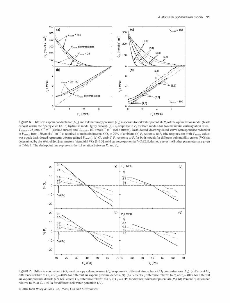
Figure 6. Diffusive vapour conductance (Gw) and xylem canopy pressure (Pc) responses to soil water potential (Ps) of the optimizationmodel (blackcurves) versus the Sperry et al. (2016) hydraulic model (grey curves). (a) Gw response to Ps for both models for two maximum carboxylation rates,Vmax25 = 25μmol s�1 m�2 (dashed curves) andVmax25 = 150μmol s�1 m�2 (solid curves). Dash-dotted ‘downregulated’ curve corresponds to reductionin Vmax25 from 150 μmol s�1 m�2 as required to maintain internal CO2 at 70% of ambient. (b) Pc response to Ps (the response for both Vmax25 valueswas equal; dash-dotted represents downregulatedVmax25). (c)Gw and (d)Pc response toPs for both models for different vulnerability curves (VCs) asdetermined by theWeibull [b,c] parameters (sigmoidal VCs [1–3,3], solid curves; exponential VCs [2,1], dashed curves).All other parameters are givenin Table 1. The dash-point line represents the 1:1 relation between Pc and Ps.

Figure 7. Diffusive conductance (Gw) and canopy xylem pressure (Pc) responses to different atmospheric CO2 concentrations (Ca). (a) PercentGw

difference relative toGw at Ca = 40 Pa for different air vapour pressure deficits (D). (b) Percent Pc difference relative to Pc at Ca = 40Pa for differentair vapour pressure deficits (D). (c) PercentGw difference relative toGw atCa = 40Pa for different soil water potentials (Ps). (d) Percent Pc differencerelative to Pc at Ca = 40 Pa for different soil water potentials (Ps).



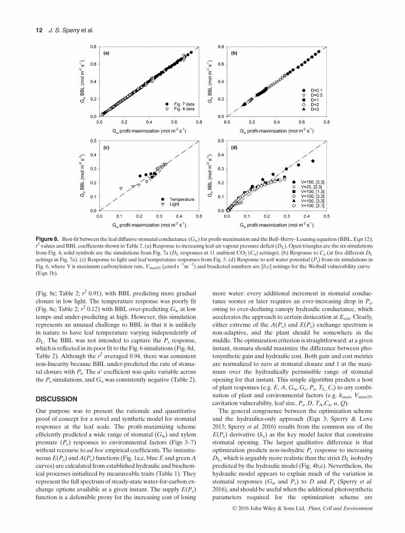
(Fig. 8c; Table 2; r2 0.91), with BBL predicting more gradualclosure in low light. The temperature response was poorly fit(Fig. 8c; Table 2; r2 0.12) with BBL over-predicting Gw at lowtemps and under-predicting at high. However, this simulationrepresents an unusual challenge to BBL in that it is unlikelyin nature to have leaf temperature varying independently ofDL. The BBL was not intended to capture the Ps response,which is reflected in its poor fit to the Fig. 6 simulations (Fig. 8d,Table 2). Although the r2 averaged 0.94, there was consistentnon-linearity because BBL under-predicted the rate of stoma-tal closure with Ps. The a′ coefficient was quite variable acrossthe Ps simulations, andGo was consistently negative (Table 2).

DISCUSSION

Our purpose was to present the rationale and quantitativeproof of concept for a novel and synthetic model for stomatalresponses at the leaf scale. The profit-maximizing schemeefficiently predicted a wide range of stomatal (Gw) and xylempressure (Pc) responses to environmental factors (Figs 3–7)without recourse to ad hoc empirical coefficients. The instanta-neousE(Pc) andA(Pc) functions (Fig. 1a,c, blueE and greenAcurves) are calculated from established hydraulic and biochem-ical processes initialized by measureable traits (Table 1). Theyrepresent the full spectrum of steady-state water-for-carbon ex-change options available at a given instant. The supply E(Pc)function is a defensible proxy for the increasing cost of losing

more water: every additional increment in stomatal conduc-tance sooner or later requires an ever-increasing drop in Pc,owing to ever-declining canopy hydraulic conductance, whichaccelerates the approach to certain desiccation at Ecrit. Clearly,either extreme of the A(Pc) and E(Pc) exchange spectrum isnon-adaptive, and the plant should be somewhere in themiddle. The optimization criterion is straightforward: at a giveninstant, stomata should maximize the difference between pho-tosynthetic gain and hydraulic cost. Both gain and cost metricsare normalized to zero at stomatal closure and 1 at the maxi-mum over the hydraulically permissible range of stomatalopening for that instant. This simple algorithm predicts a hostof plant responses (e.g. E, A,Gw, Gc, Pc, TL, Ci) to any combi-nation of plant and environmental factors (e.g. kmax, Vmax25,cavitation vulnerability, leaf size, Ps, D, TA,Ca, u, Q).

The general congruence between the optimization schemeand the hydraulics-only approach (Eqn 3; Sperry & Love2015; Sperry et al. 2016) results from the common use of theE(Pc) derivative (kc) as the key model factor that constrainsstomatal opening. The largest qualitative difference is thatoptimization predicts non-isohydric Pc response to increasingDL, which is arguably more realistic than the strictDL isohydrypredicted by the hydraulic model (Fig. 4b,c). Nevertheless, thehydraulic model appears to explain much of the variation instomatal responses (Gw and Pc) to D and Ps (Sperry et al.2016), and should be useful when the additional photosyntheticparameters required for the optimization scheme are

Figure 8. Best-fit between the leaf diffusive stomatal conductance (Gw) for profit-maximation and theBall–Berry–Leuning equation (BBL, Eqn 12);r2 values andBBL coefficients shown inTable 2. (a) Response to increasing leaf-air vapour pressure deficit (DL). Open triangles are the six simulationsfrom Fig. 4; solid symbols are the simulations from Fig. 7a (DL responses at 11 ambient CO2 (Ca) settings). (b) Response to Ca (at five different DL

settings in Fig. 7a). (c) Response to light and leaf temperature responses from Fig. 5. (d) Response to soil water potential (Ps) from six simulations inFig. 6, where V is maximum carboxylation rate, Vmax25 (μmol s�1m�2) and bracketed numbers are [b,c] settings for the Weibull vulnerability curve(Eqn 1b).



unavailable, and CO2 and light do not vary substantially. All ofits advantages in capturing the isohydric-to-anisohydric spec-trum (e.g. Fig. 6d; and see Sperry et al. 2016), and the coupledresponses toDL and Ps (Figs 4 & 6), carry over in the optimiza-tion model. However, the optimization model captures themost complete suite of stomatal responses because Gw re-sponds to A. This allows it to predict additional responses toTA, Q and Ca (Figs 5 & 7).The comparison to the Ball–Berry–Luening (Leuning 1995)

model (BBL) represents a ‘zero-order’ test of the optimizationmodel. The BBL fit was essentially perfect for the stomatal re-sponse toDL andCa (Figs 4 & 7). This result was anticipated bytheBBL form of theoretical derivations for profit maximization(Wolf et al. 2016). TheBBL congruency suggests that the trendsin Figs 4 (closure at highDL) and 7 (opening at low Ca, closureat high Ca) are quantitatively as well as qualitatively consistentwith observations. The advantage of the optimization approachover BBL (or other empirical models) is the absence of ad hocfitting parameters (e.g. Table 2) and its basis in trait and pro-cess. Even more importantly, the optimization model appliesequally well to dry soil (e.g. Fig. 6a,c). The BBL model lacksany parameter for capturing the Gw response to drying soil(Eqn 12; Darmour et al. 2010), and under-predicts stomatal clo-sure relative to the optimization model (Fig. 8d). This criticaldefect is often patched up in ecosystem models by the additionof more ad hoc functions and coefficients (Jarvis 1976; Powellet al. 2013). But the optimization model provides a simplerand more powerful alternative. Its integration of photosynthe-sis and hydraulics predicts not only gas exchange and energybalance, but the accompanying water relations and hydraulicstatus. As the rapidly growing literature on drought inducedtree mortality suggests, metabolic, temperature and hydraulicstresses are inextricably intertwined during drought(McDowell et al. 2008; Rowland et al. 2015; Anderegg et al.2016). Models need to represent their integration to best pre-dict responses to environmental change (McDowell et al. 2013).Additional evidence for the optimization model comes from

its prediction of a tightly coupled coordination between kmax,Gmax and Vmax25 (Fig. 3). This is consistent with an abundanceof data showing a positive relationship between kleaf and Vmax

(Clearwater & Meinzer 2001; Brodribb et al. 2002; Brodribbet al. 2005; Brodribb et al. 2007; Campanello et al. 2008;Brodribb 2009; Brodribb & Feild 2010; Limousin et al. 2013;Novick et al. 2016). The coordination between hydraulic andphotosynthetic capacity emerges from the assumption thatCi/Ca is maintained at a set value under favourable conditions.A constant Ci/Ca target was also proposed as a carbon-for-water transport optimization criterion by Prentice et al.(2014), and previous modelling has demonstrated its theoreti-cal link to plant hydraulic properties (Katul et al. 2003). Theoptimal kmax settings also correspond to leaf area-specifichydraulic conductances within the measured range (5–65mmol s�1m�2MPa; assuming leaves are 25% of plant resis-tance at full hydration; Sack&Tyree 2005). The further predic-tion that kmax should increase with vulnerability to cavitation(Fig. 3b) is consistent with generally observed trends (Gleasonet al. 2015). Interestingly, however, this trend is predicted inde-pendently of any safety versus efficiency trade-off at the xylem

level. Instead, it emerges from vulnerable xylem limiting thesoil-canopy ΔP, thus requiring higher kmax to achieve the Gw

required to keep A and Ci at optimal levels (Fig. 3a).Our optimization criterion, that of instantaneously maximiz-

ing carbon gain (β) minus hydraulic cost (θ; Eqn 11; Wolf et al.2016), is importantly different from the Cowan–Farquharmaximization of carbon gain for a fixed amount of water loss.The ∂E/∂A= λ′ target for stomatal regulation in the Cowan–Farquhar scheme is unspecified, which prevents direct compar-ison ofGw. But the response shape can be compared by settingλ′= ∂E/∂A at the initialGw for profit maximization, and plottingthe alternative Gw trajectory that maintains λ′ instead of profitmaximization. When soil is wet, the Gw response to DL can bequite similar (Fig. 9a, Ps = 0 curves; Vmax25 = 100μmol s�1m�2,TA=30 °C), which is consistent with support for a near-constant ∂E/∂A over diurnal time frames of favourable soilmoisture (e.g. Farquhar et al. 1980). It is also consistent with rel-atively low hydraulic cost under these conditions. However, assoil dries, the new λ′ setting (reduced to match the lower initialGw) predicts more severe closure withDL (even toGw≈ 0) andmore conservative water use versus profit maximization, whichpredicts ∂E/∂A should rise withDL (rather than stay constant).Such a rise has been observed (Thomas et al. 1999; but seeBuckley et al. 2016) and is also predicted if TL increases withDL beyond the photosynthetic optimum (simulations notshown). The response to Ps (constantD) is dramatically differ-ent in the two schemes: maintaining λ′ results in no stomatalclosure and premature hydraulic failure (Fig. 9b, desiccationat the asterisk). Profit maximization predicts a strong closureresponse (and declining ∂E/∂A) because of the rising cost ofextracting water from drying soil. The reduction in λ′with driersoil has been anticipated and observed, although its a priorispecification remains very difficult (Cowan 1982; Makala et al.1996; Thomas et al. 1999; Manzoni et al. 2011; Manzoni et al.2013). The CO2 response is also dramatically different: as Ca

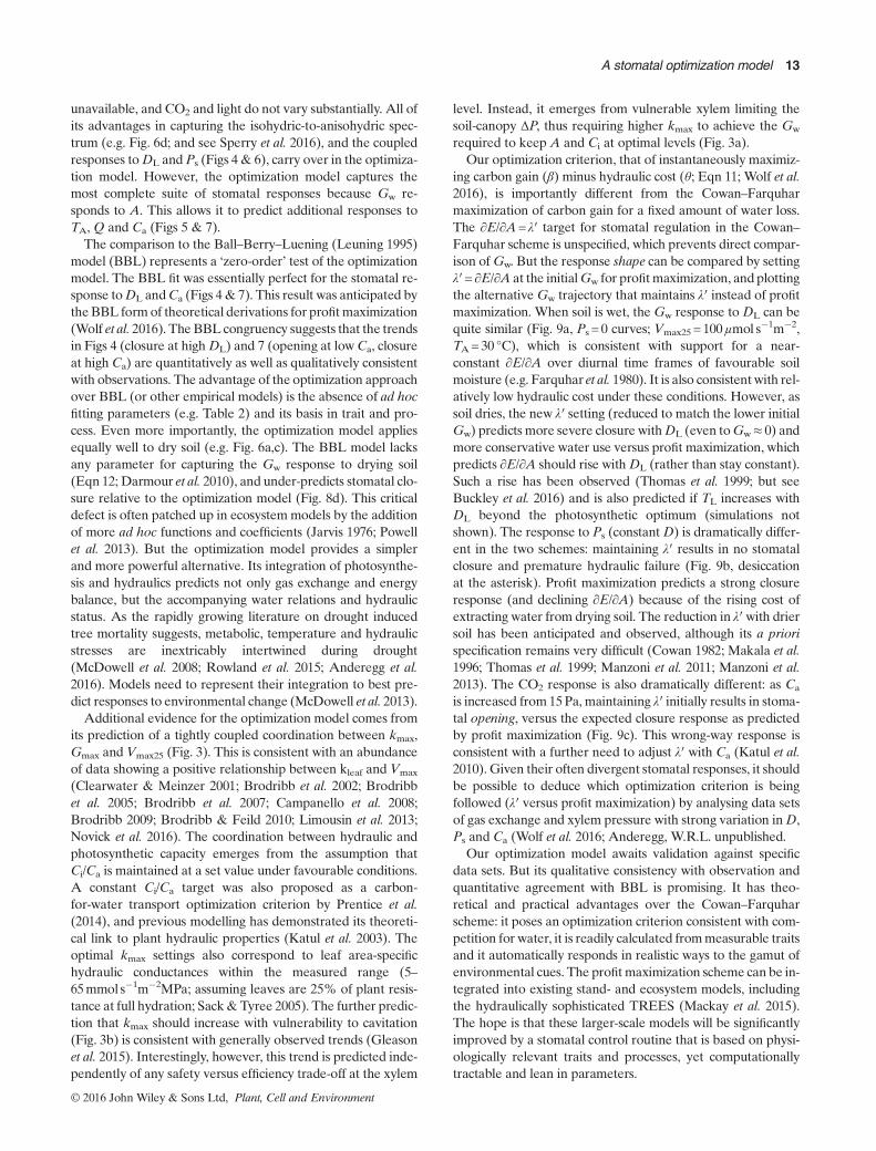
is increased from 15Pa, maintaining λ′ initially results in stoma-tal opening, versus the expected closure response as predictedby profit maximization (Fig. 9c). This wrong-way response isconsistent with a further need to adjust λ′ with Ca (Katul et al.2010). Given their often divergent stomatal responses, it shouldbe possible to deduce which optimization criterion is beingfollowed (λ′ versus profit maximization) by analysing data setsof gas exchange and xylem pressure with strong variation inD,Ps and Ca (Wolf et al. 2016; Anderegg, W.R.L. unpublished.

Our optimization model awaits validation against specificdata sets. But its qualitative consistency with observation andquantitative agreement with BBL is promising. It has theo-retical and practical advantages over the Cowan–Farquharscheme: it poses an optimization criterion consistent with com-petition for water, it is readily calculated frommeasurable traitsand it automatically responds in realistic ways to the gamut ofenvironmental cues. The profit maximization scheme can be in-tegrated into existing stand- and ecosystem models, includingthe hydraulically sophisticated TREES (Mackay et al. 2015).The hope is that these larger-scale models will be significantlyimproved by a stomatal control routine that is based on physi-ologically relevant traits and processes, yet computationallytractable and lean in parameters.



ACKNOWLEDGMENTS

We thank Plant Cell and Environment for this special issueinvitation. Funding was from NSF-IOS-1450650 and NSF-IOS-1450679. Dr. Gabriel Katul (Duke University) generously

provided feedback on an early draft, and we benefitted frominformative discussions with Fred Adler (University of Utah).Belinda Medlyn (Western Sydney University) and an anony-mous referee provided excellent review feedback.

REFERENCES

von Allmen A.I., Sperry J.S. & Bush S.E. (2015) Contrasting whole-tree wateruse, hydraulics, and growth in a co-dominant diffuse-porous vs. ring-porousspecies pair. Trees Structure and Function 29, 717–728.

AndereggW.R.L., Flint A., Huang C., Flint L., Berry J.A., Davis F., Sperry J.S. &Field C.B. (2015) Tree mortality predicted from drought-induced vasculardamage. Nature Geoscience 8, 367–371.

AndereggW.R.L., Klein T., BartlettM., Sack L., Pellegrini B., Choat B.& JansenS. (2016) Meta-analysis reveals that hydraulic traits explain cross-speciespatterns of drought-induced tree mortality across the globe. Proceedings ofthe National Academy of Sciences of the United States of America 113,5024–5029.

Bernacchi C.J., Singsaas E.L., Pinentel C., Portis A.R. & Long S.P. (2001)Improved temperature response functions for models of Rubisco-limitedphotosynthesis. Plant, Cell & Environment 24, 253–259.

Bonan G.B., Williams M., Fisher R.A. & Oleson K.W. (2014) Modeling stomatalconductance in the earth system: linking leaf water-use efficiency and watertransport along the soil-plant-atmosphere continuum. Geosciences ModelDevelopment 7, 2193–2222.

Brodribb T.J. (2009) Xylem hydraulic physiology: the functional backbone ofterrestrial plant productivity. Plant Science 177, 245–251.

Brodribb T.J. & Feild T.S. (2010) A surge in leaf photosynthetic capacity duringearly angiosperm diversification. Ecology Letters 13, 175–183.

Brodribb T.J., Feild T.S. & Jordan G.J. (2007) Leaf maximum photosyn-thetic rate and venation are linked by hydraulics. Plant Physiology 144,1890–1898.

Brodribb T.J., Holbrook N.M. &Gutierrez M.V. (2002) Hydraulic and photosyn-thetic co-ordination in seasonally dry tropical forest trees. Plant, Cell &Environment 25, 1435–1444.

Brodribb T.J., HolbrookN.M., Zwieniecki M.A.& Palma B. (2005) Leaf hydrau-lic capacity in ferns, conifers, and angiosperms: impacts on photosyntheticmaxima. New Phytologist 165, 839–846.

Buckley T.N., Sack L. & Farquhar G.D. (2016) Optimal plant water economy.Plant, Cell & Environment. DOI:10.1111/pce.12823.

Campanello P.I., Gatti M.G.&GoldsteinG. (2008) Coordination betweenwater-transport efficiency and photosynthetic capacity in canopy tree species atdifferent growth irradiances. Tree Physiology 28, 85–94.

Campbell G.S. &Norman J.N. (1998)An Introduction toEnvironmental Biophys-ics 2nd edn. Springer, New York.

ClearwaterM.J. &Meinzer F.C. (2001) Relationship between hydraulic architec-ture and leaf photosynthetic capacity in nitrogen-fertilized Eucalyptus grandistrees. Tree Physiology 21, 683–690.

Collatz G.J., Ball J.T., Grivet C. & Berry J.A. (1991) Physiological and environ-mental regulation of stomatal conductance, photosynthesis and transpiration:a model that includes a laminar boundary layer. Agricultural and ForestMeteorology 54, 107–136.

Collatz G.J., Ribas-Carbo M. & Berry J.A. (1992) Coupled photosynthesis-stomatal conductancemodel for leaves ofC4 plants.Australian Journal of PlantPhysiology 19, 519–538.

Cowan I.R. (1982) Regulation of water use in relation to carbon gain in higherplants. In Physiological Plant Ecology II. Encyclopedia of Plant Physiology(eds Lange O.L., Nobel P.S., Osmond C.B. & Ziegler H.), Vol. 12B,pp. 589–613. Springer-Verlag, Berlin.

Cowan I.R. & Farquhar G.D. (1977) Stomatal function in relation to leafmetabolism and environment. In Integration of Activity in the Higher Plant(ed Jennings D.H.), pp. 471–505. Cambridge University Press, Cambridge.

Darmour G., Simonneau T., Cochard H. & Urban L. (2010) An overview ofmodels of stomatal conductance at the leaf level. Plant, Cell & Environment33, 1419–1438.

Farquhar G.D., Schulze E.D. & Kuppers M. (1980) Responses to humidity bystomata of Nicotiana glauca L. and Corylus avellana L. are consistent withthe optimization of carbon dioxide uptake with respect to water loss.Australian Journal of Plant Physiology 7, 315–327.

Feild C.B. & Holbrook N.M. (1989) Catastrophic xylem failure: life at the brink.Trends in Ecology and Evolution 4, 124–126.

Figure 9. The response of leaf diffusive conductance (Gw) for profitmaximization (black curves) versus the constrained optimization ofCowan & Farquhar (1977; grey curves) where marginal water useefficiency (λ′= ∂E/∂A) is constant at the initial value for profitmaximization. (a) The response to leaf-air vapour pressure deficit (DL)at three soil water potentials (Ps = 0,�0.75,�1.5MPa). (b)Response toPs; asterisk denotes point of hydraulic failure and canopy desiccation.(c) Response to ambient CO2 concentration (Ca).



http://dx.doi.org/10.1111/pce.12823

van Genuchten M.T. (1980) A closed form equation for predicting the hydraulicconductivity of unsaturated soils. Soil Science Society of America Journal 44,892–898.

Givnish T.J. (1986) Optimal stomatal conductance, allocation of energy betweenleaves and roots, and the marginal cost of transpiration. InOn the Economy ofPlant Form and Function (ed Givnish T.J.), pp. 171–213. CambridgeUniversityPress, Cambridge.

Gleason S.M., Westoby M., Jansen S., Choat B., Hacke U.G., Pratt R.B., …Zanne A.E. (2015) Weak tradeoff between xylem safety and xylem-specifichydrualic efficiency across the world’s woody plant species. New Phytologist209, 123–136.

Hetherington A.M. & Woodward F.I. (2003) The role of stomata in sensing anddriving environmental change. Nature 424, 901–908.

Jarvis P.G. (1976) The interpretation of the variations in leaf water potential andstomatal conductance found in canopies in the field.Philosophical Transactionsof the Royal Society London, Series B 273, 593–610.

Katul G.G., Leuning R. & Oren R. (2003) Relationship between plant hydraulicand biochemical properties derived from a steady-state coupled water andcarbon transport model. Plant, Cell & Environment 26, 339–350.

Katul G.G., Manzoni S., Palmroth S. & Oren R. (2010) A stomatal optimizationtheory to describe the effects of atmospheric CO2 on leaf photosynthesis andtranspiration. Annals of Botany 105, 431–442.

Kukowski K., Schwinning S. & Schwartz B. (2013) Hydraulic responses toextreme drought conditions in three co-dominant tree species in shallow soilover bedrock. Oecologia 171, 819–830.

Leuning R. (1995) A critical appraisal of a coupled stomatal-photosynthesismodel for C3 plants. Plant, Cell & Environment 18, 339–357.

LeuningR. (2002) Temperature dependence of two parameters in a photosynthe-sis model. Plant, Cell & Environment 25, 1205–1210.

Limousin J., Bickford C., Dickman L., Pangle R., Hudson P., Boutz A., … Mc-Dowell N. (2013) Regulation and acclimation of leaf gas exchange in a piñon-juniper woodland exposed to three different precipitation regimes. Plant, Cell& Environment 36, 1812–1825.

Mackay D.S., Roberts D.E., Ewers B.E., Sperry J.S., McDowell N. & PockmanW. (2015) Interdependence of chronic hydraulic dysfunction and canopyprocesses can improve integrated models of tree response to drought. WaterResources Research 51. DOI:10.1002/2015WR017244.

Makala A., Berninger F. &Hari P. (1996)Optimal control of gas exchange duringdrought: theoretical analysis. Annals of Botany 77, 461–468.

Manzoni S., Vico G., Katul G., Fay P.A., Polley W., Palmroth S. & Porporato A.(2011) Optimizing stomatal conductance for maximum carbon gain under wa-ter stress: a meta-analysis across plant functional types and climates. FunctionalEcology 25, 456–467.

Manzoni S., Vico G., Porporato A., Palmroth S. & Katul G. (2013) Optimizationof stomatal conductance for maximum carbon gain under dynamic soil mois-ture. Advances in Water Resources 62, 90–105.

McDowell N., Fisher R.A., Xu C., Domec J.C., Holtta T., Mackay D.S., …Pockman W.T. (2013) Evaluating theories of drought-induced vegetationmortality using a multimodel-experimental framework. New Phytologist 200,304–321.

McDowell N., Pockman W.T., Allen C.D., Breshears D.D., Cobb N., Kolb T.,…Yepez E.A. (2008)Mechanisms of plant survival and mortality during drought.Why do someplants survive while others succumb to drought?NewPhytologist178, 719–739.

Medlyn B.E., DreyerE., EllsworthD.S., ForstreuterM., Harley P.C.,KirschbaumM.U.F., … Loustau D. (2002) Temperature response of parameters of abiochemically based model on photosynthesis. II. A review of experimentaldata. Plant, Cell & Environment 25, 1167–1179.

Medlyn B.E., Duursma R.A., Eamus D., Ellsworth D.S., Prentice I.C., BartonC.V.M., … Wingate L. (2011) Reconciling the optimal and empirical ap-proaches to modelling stomatal conductance. Global Change Biology 17,2134–2144.

Morison J.I.L. (1987) Intercellular CO2 concentration and stomatal response toCO2. In Stomatal Function (eds Zeiger E., Cowan I.R. & Farquhar G.D.),pp. 229–251. Stanford University Press, Stanford.

Novick K.R.,Miniat C.F. & Vose J.M. (2016) Drought limitations to leaf-level gasexchange: results from a model linking stomatal optimization and cohesion–tension theory. Plant, Cell & Environment 39, 583–596.

NeufeldH.S., GrantzD.A.,Meinzer F.C.,GoldsteinG., CrisostoG.M.&CrisostoC. (1992) Genotypic variability in vulnerability of leaf xylem to cavitation inwater-stressed and well-irrigated sugarcane. Plant Physiology 100, 1020–1028.

Paul M.J. & Foyer C.H. (2001) Sink regulation of photosynthesis. Journal ofExperimental Botany 52, 1383–1400.

Powell T., GalbraithD., Christoffersen B., Harper A., Imbuzeiro H., Rowland L.,… Moorcroft P. (2013) Confronting model predictions of carbon fluxes withmeasurements of Amazon forests subjected to experimental drought. NewPhytologist 200, 350–365.

Prentice I.C., DongN., Gleason S.M.,MaireV.&Wright I.J. (2014)Balancing thecosts of carbon gain and water transport: testing a new theoretical frameworkfor plant functional ecology. Ecology Letters 17, 82–91.

Rowland L., da Costa A.C.L., Galbraith D.R., Oliveira R.S., Binks O.J., OliveiraA.A., … Meir P. (2015) Death from drought in tropical forests is triggered byhydraulics not carbon starvation. Nature 528, 119–122.

Sack L. & Tyree M.T. (2005) Leaf hydraulics and its implications in plantstructure and function. In Vascular Transport in Plants (eds Holbrook N.M.& Zwieniecki M.A.), pp. 93–114. Elsevier/Academic Press, Oxford.

Schulze E.D. & Hall A.E. (1982) Stomatal responses water loss and CO2-assimi-lation rates of plant in contrasting environments. In Physiological PlantEcology II. Water Relations and Carbon Assimilation (eds Lange O.L., NobelP.S., Osmond C.B. & Ziegler H.), pp. 181–230. Springer Verlag, Berlin.

Sparks J.P. & Black R.A. (1999) Regulation of water loss in populations ofPopulus trichocarpa: the role of stomatal control in preventing xylem cavita-tion. Tree Physiology 19, 453–459.

Sperry J.S.,Adler F.R., Campbell G.S. &Comstock J.P. (1998) Limitation of plantwater use by rhizosphere and xylem conductance: results from a model. Plant,Cell & Environment 21, 347–359.

Sperry J.S. & LoveD.M. (2015) Tansley review:What plant hydraulics can tell usabout plant responses to climate-change droughts.New Phytologist 207, 14–27.

Sperry J.S., Wang Y., Wolfe B., Mackay D.S., AndereggW.R.L., McDowell N.G.& Pockman W.T. (2016) Pragmatic hydraulic theory predicts stomatal re-sponses to climatic water deficits. New Phytologist 212, 577–589.

ThomasD.S., EamusD.&Bell D. (1999)Optimization theory of stomatal behav-iour II. Stomatal responses of several tree species of north Australia to changesin light, soil and atmospheric water content and temperature. Journal ofExperimental Botany 50, 393–400.

Tombesi S., Nardini A., Frioni T., Soccolini M., Zadra C., Farinelli D.,… PalliottiA. (2015) Stomatal closure is induced by hydraulic signals and maintained byABA in drought-stressed grapevine. Scientific Reports 5, 12449.

Tyree M.T. & Sperry J.S. (1988) Do woody plants operate near the point ofcatastrophic xylem dysfunction caused by dynamic water stress? Answers froma model. Plant Physiology 88, 574–580.

Williams M., Rastetter E.B., Fernandes D.N., GouldenM.L., Wofsy S.C., ShaverG.R.,… Nadelhoffer K.J. (1996) Modelling the soil-atmosphere continuum ina Quercus-Acer stand at Harvard Forest: the regulation of stomatal conduc-tance by light, nitrogen and soil/plant hydraulic properties. Plant, Cell & Envi-ronment 19, 911–927.

Wolf A., Anderegg W.R.L. & Pacala S. (2016) Optimal stomatal behavior withcompetition for water and risk of hydraulic impairment. Proceedings of theNational Academy of Sciences of the United States of America. In Press.

Wong S.C., Cowan I.R.& FarquharG.D. (1979) Stomatal conductance correlateswith photosynthetic capacity. Nature 282, 424–426.

Received 11 July 2016; received in revised form 28 September 2016;accepted for publication 6 October 2016

SUPPORTING INFORMATION

Additional Supporting Information may be found in the onlineversion of this article at the publisher’s web-site:

Figure S1. Examples of how specific plant- and environmentalparameters shifts the gain-cost (β–θ) optimization.Figure S2. Example of how an exponential vulnerability curveshifts the gain-cost (β–θ) optimization in wet versus dry soil.



http://dx.doi.org/10.1002/2015WR017244

Predicting stomatal responses to the environment from …€¦ · Original Article Predicting...

Documents

Transcript of Predicting stomatal responses to the environment from …€¦ · Original Article Predicting...