PREDICTING PEDESTRIAN CRASH OCCURRENCE AND …
21
PREDICTING PEDESTRIAN CRASH OCCURRENCE AND INJURY SEVERITY IN 1 TEXAS USING TREE-BASED MACHINE LEARNING MODELS 2 3 4 Bo Zhao, M.Sc. 5 Graduate Research Assistant 6 Department of Plant Biology 7 The University of Texas at Austin 8 Austin, TX, 78712 9 [email protected] 10 11 Natalia Zuniga-Garcia, Ph.D. 12 Postdoctoral Fellow 13 Department of Civil, Architectural and Environmental Engineering 14 The University of Texas at Austin 15 Austin, TX, 78712 16 [email protected] 17 18 Lu Xing, M.Sc. 19 Graduate Research Assistant 20 Department of Civil, Architectural and Environmental Engineering 21 The University of Texas at Austin 22 Austin, TX, 78712 23 [email protected] 24 25 Kara M. Kockelman, Ph.D., P.E. 26 (Corresponding Author) 27 Professor and Dewitt Greer Centennial Professor of Transportation Engineering 28 Department of Civil, Architectural and Environmental Engineering 29 The University of Texas at Austin – 6.9 E. Cockrell Jr. Hall 30 Austin, TX, 78712-1076 31 [email protected] 32 33 34 Under review for presentation at the 101st Annual Meeting of the Transportation Research 35 Board and for publication in Transportation Research Record 36 37 38 ABSTRACT 39 This study investigates the frequency and injury severity of pedestrian crashes across Texas using 40 tree-based machine learning models. Ten years of police records are used along with roadway 41 inventory and other sources to map more than 78,000 pedestrian crashes over 700,000 road 42 segments along with road design, land use, transit stops, and hospital location and weather 43 information. Methods such as random forests (RF), gradient boosting (LightGBM and XGBoost), 44 and Bayesian additive regression trees (XBART) are applied and compared. The crash frequency 45 models indicate that highway design variables significantly positively impact crash frequencies. 46
Transcript of PREDICTING PEDESTRIAN CRASH OCCURRENCE AND …

PREDICTING PEDESTRIAN CRASH OCCURRENCE AND INJURY SEVERITY IN 1
TEXAS USING TREE-BASED MACHINE LEARNING MODELS 2
3
4
Bo Zhao, M.Sc. 5
Graduate Research Assistant 6
Department of Plant Biology 7
The University of Texas at Austin 8
Austin, TX, 78712 9
11
Natalia Zuniga-Garcia, Ph.D. 12
Postdoctoral Fellow 13
Department of Civil, Architectural and Environmental Engineering 14
The University of Texas at Austin 15
Austin, TX, 78712 16
18
Lu Xing, M.Sc. 19
Graduate Research Assistant 20
Department of Civil, Architectural and Environmental Engineering 21
The University of Texas at Austin 22
Austin, TX, 78712 23
25
Kara M. Kockelman, Ph.D., P.E. 26
(Corresponding Author) 27
Professor and Dewitt Greer Centennial Professor of Transportation Engineering 28
Department of Civil, Architectural and Environmental Engineering 29
The University of Texas at Austin – 6.9 E. Cockrell Jr. Hall 30
Austin, TX, 78712-1076 31
33
34
Under review for presentation at the 101st Annual Meeting of the Transportation Research 35
Board and for publication in Transportation Research Record 36
37
38
ABSTRACT 39
This study investigates the frequency and injury severity of pedestrian crashes across Texas using 40
tree-based machine learning models. Ten years of police records are used along with roadway 41
inventory and other sources to map more than 78,000 pedestrian crashes over 700,000 road 42
segments along with road design, land use, transit stops, and hospital location and weather 43
information. Methods such as random forests (RF), gradient boosting (LightGBM and XGBoost), 44
and Bayesian additive regression trees (XBART) are applied and compared. The crash frequency 45
models indicate that highway design variables significantly positively impact crash frequencies. 46

Zhao, Zuniga-Garcia, Xing, and Kockelman
Increments in total or fatal crash counts are related to a higher number of lanes, while higher speed 1
and greater median and shoulder widths lead to fewer crash frequencies. Other variables such as 2
proximity to schools, the number of transit stops, and population and job density increased 3
pedestrian crash occurrences. Pedestrian severity models found that a high speed limit significantly 4
increases the likelihood of pedestrian fatalities and severe injuries, and intoxicated drivers and 5
pedestrians lead to more severe injuries. Also, pedestrian crashes are more likely to be severe and 6
fatal at night and in areas with poor lighting conditions. An analysis of the vehicle type found that 7
light-duty trucks (pickups, SUVs, and vans) also increase pedestrian severity. The comparison of 8
the four models indicates that they performed similarly in predicting crash occurrences, with 9
LightGBM showing significantly lower computational time. While for crash injury severity 10
models, XBART obtained a higher precision value but with a significantly high computational 11
time. 12
13
Keywords: Pedestrian safety; Crash counts; Injury severity; Machine learning; Random forest; 14
Gradient boosting; Bayesian Additive Regression Trees (BART). 15

Zhao, Zuniga-Garcia, Xing, and Kockelman
1
INTRODUCTION 1
Walking is the most environmentally friendly form of transportation and has numerous health 2
benefits [1], [2]. However, walking has become increasingly risky in recent years. During the ten 3
years 2010-2019, the number of U.S. pedestrian fatalities increased by 46% [3], while the total 4
walking miles traveled risen approximately 16% from 2009 to 2017 [4]. Walking trips accounted 5
for 10% of the total trips taken in the nation in 2017, but pedestrians represented 16% of total 6
traffic fatalities in the same year [3], [5]. This indicates that pedestrians experience a higher risk 7
of fatality than motorists based on their exposure level. Furthermore, the risk of injury when 8
walking is four times more than when driving a car [6]. There were 1.14 pedestrian fatalities per 9
100,000 people in Texas during 2019 [3], a rate 26% higher than the national average of 0.9. This 10
study aims to investigate pedestrian-involved crashes in Texas using ten years of data from police 11
records to determine which factors are critical to developing countermeasures for safer roadways. 12
13
Several studies have been conducted to examine the factors contributing to the frequency and 14
severity of pedestrian crashes. Research findings suggest that pedestrian crash frequency can be 15
influenced by roadway design characteristics, demographic, land use, and environmental, and 16
weather conditions [7]–[11]. Several studies are based on macro-level information, with data 17
aggregated at area levels like traffic analysis zones, census tracts, and zip code, while studies using 18
micro-level aggregation, such as intersection and street segments, are more limited. Macro-level 19
studies are useful to understand a city or state as a complex system. However, conducting micro-20
level studies can be crucial for the implementation of countermeasures for safety improvements. 21
Using macro-level data at the Census tract, Wier et al. (2009) found that statistically significant 22
predictors of vehicle-pedestrian collisions including traffic volume, employee and resident 23
populations, arterial streets without public transit, proportions of the land area zoned for 24
neighborhood commercial use, and residential-neighborhood commercial use, land area, the 25
proportion of people living in poverty, and proportion of people aged 65 and over are statistically 26
significant predictors of vehicle-pedestrian collisions. The micro-level analysis includes the work 27
by Lee and Abdel-Aty (2005). They analyzed pedestrian crashes at intersections in Florida using 28
negative binomial (NB) and log-linear models. They found that middle-aged male drivers and 29
pedestrians were correlated to more pedestrian crashes than the other age and gender groups. With 30
data aggregated at two different road segment levels, Vahedi Saheli and Effati (2021) used four 31
count-based regression models (Poisson, NB, and their zero-inflated extensions) to show that 32
residential, commercial, governmental, institutional, utility, and religious land uses have decisive 33
impacts on the increase of pedestrian crash frequency. 34
35
Pedestrian injury severity analysis has also been widely used to the analyze factors leading to 36
pedestrian injuries and fatalities. Tay et al. (2011) estimated a multinomial logit (MNL) model to 37
identify the factors determining the severity of pedestrian-vehicle crashes. They found that fatal 38
and serious crashes were associated with collisions involving heavy vehicles, drunk drivers, males 39
or those under the age of 65, on high-speed roads, with inclement weather conditions, at night, on-40
road links, or on wider roads. Lee and Abdel-Aty (2005) used an ordered probit (OP) model and 41
similarly found that pedestrian injury severity is closely related to pedestrians’ physical condition 42
(age and alcohol or drug use), the speed at the time of crashes, location of crashes, the presence of 43
traffic control, weather and lighting conditions, and vehicle type. Kim et al. (2008) used 44
heteroskedastic ordered probit (HOP) and MNL models to explore injury severity. The results 45
show that pedestrian age induces heteroskedasticity, which affects the probability of fatal injury, 46

Zhao, Zuniga-Garcia, Xing, and Kockelman
2
and the effect grows more pronounced with increasing age past 65. They found that the HOP model 1
provides a better fit than the MNL model. 2
3
While extensive research has been developed using traditional frequency and severity models, 4
studies using machine learning (ML) methods are limited. ML methods have been applied recently 5
in the transportation safety literature to provide more accurate prediction models due to their ability 6
to deal with more complex functions [16], [17]. Tree-based ML models are popular methods to 7
make predictions. Ensemble tree models implementing bagging or boosting approaches usually 8
outperform traditional statistically-based prediction models due to the informative and deliverable 9
prediction. Examples of tree-based ML analysis include the use of random forest (FR) to evaluate 10
the injury severity in pedestrian-bus crashes [18] and extreme gradient boosting (XGBoost) was 11
used by Guo et al. (2021) to study older pedestrian crash severity. However, there is a lack of 12
studies developing crash count models for pedestrian frequency prediction using tree-based ML 13
models. There is also a need for model performance comparison across other models, such as light 14
gradient boosting machine (LightGBM) and Bayesian additive regression tree (BART). In this 15
study, four different tree-based machine learning models (RF, XGBoost, LightGBM, and 16
accelerated BART) are applied to identify major factors contributing to pedestrian-vehicle crash 17
occurrences and pedestrian injury severity. 18
DATA DESCRIPTION 19
Several data sources are used in this study. Crash records from 2010 to 2019 are obtained from the 20
Texas Department of Transportation (TxDOT) Crash Records Information System (CRIS). The 21
CRIS system comprises records of police reports generated in all 254 Texas counties and the 22
hundreds of municipalities therein. Variables within the database characterize crashes according 23
to time, location, severity, and road conditions. Also, the TxDOT Roadway Inventory database 24
was used to obtain road-specific attributes. 25
26
The CRIS data was spatially matched with land use, population, job, rainfall, and other location 27
features (schools, hospitals, transit stops) to examine the association between pedestrian crash 28
counts and various contributing factors along Texas roads. Census tract-level population and job 29
data were obtained from the 2010 US Census and Longitudinal Employer-Household Dynamics 30
(LEHD) dataset respectively. Road segments were matched with the closest census tract centroid 31
using the ArcGIS spatial join routine. Data were normalized by the area of census tracts. Other 32
data sources include annual rainfall data (1981–2010) from the Texas Water Board, school 33
locations from the Texas Education Agency, hospital locations from the Homeland Infrastructure 34
Foundation, and transit stop locations from OpenStreetMap. ArcGIS Spatial Analysis tools were 35
utilized to calculate numbers of transit stops and Euclidean distances from each road segment to 36
the nearest schools and hospitals. 37
38
During the period between 2010 and 2019, a total of 5,631,223 crashes were recorded in the CRIS 39
system. Among these crashes, 78,497 involved collisions or avoidance of pedestrians and a total 40
of 72,243 pedestrians were involved. The distribution of the pedestrian crashes by fatality is 41
described as follows: 5.9 % pedestrians were not injured, 33.0% presented a possible injury, 36.1% 42
suffered a non-incapacitating injury, 15.8% were incapacitated, and 7.7% were killed, with 1.5% 43
of unknown severity. Table 1 shows summary statistics of the variables at the road-segment level. 44

Zhao, Zuniga-Garcia, Xing, and Kockelman
3
TABLE 1: Summary statistics of variables for road segments across Texas 1
Variables Mean Std. Dev Min Median Max
Number of pedestrian crashes 0.08 0.65 0.00 0.00 115
Number of fatal pedestrian crashes 0.01 0.10 0.00 0.00 10.00
Segment length (in miles) 0.43 0.81 0.00 0.19 44.24
Number of lanes 2.23 0.78 1.00 2.00 14.00
Median width (in feet) 1.74 11.79 0.00 0.00 519.00
Average shoulder width (in feet) 1.41 3.62 0.00 0.00 42.00
On-system road 0.23 0.42 0.00 0.00 1.00
Indicator of curvature 0.11 0.31 0.00 0.00 1.00
Curve length (in meters) 21.68 125.77 0.00 0.00 9,630.57
Curve angle (degrees) 3.54 12.95 0.00 0.00 331.80
Average daily traffic (ADT) per lane 888 2,366 0.00 165 92,090
Percentage of truck ADT 5.96 7.22 0.00 3.20 95.80
Daily VMT (DVMT) 1,035 7,319 0.00 54 793,942
Speed limit (mph) 56.97 28.69 10.00 0.00 85.00
Rural (pop. < 5000) 0.41 0.49 0.00 0.00 1.00
Small urban (pop: 5000–49999) 0.10 0.30 0.00 0.00 1.00
Urbanized (pop: 50000–199999) 0.09 0.29 0.00 0.00 1.00
Large urbanized (pop: 200000+) 0.40 0.49 0.00 0.00 1.00
Population density (per sq. mile) 1,672 2,275 0.00 636 55,240
Job density (per sq. mile) 805 3,285 0.00 140 130,011
Average yearly precipitation (1981–2010)
(inches) 36.48 11.52 8.00 37.00 61.00
Distance to nearest hospital (miles) 6.82 7.28 0.00 3.97 98.21
Distance to nearest school (miles) 2.08 3.09 0.01 0.74 53.95
Presence of transit stop within 100-meter buffer 0.01 0.08 0.00 0.00 1.00
Number of transit stops within 100-meter buffer 0.01 0.20 0.00 0.00 27.00
METHODOLOGY 2
This study investigates the performance of tree-based ensemble machine learning models in 3
predicting pedestrian occurrence and severity in roadway segments in Texas. An outline of the 4
proposed model training and sensitivity analysis process is presented in Figure 1. First, the 5
pedestrian crash dataset is split into training and test sets. After fitting the models on the training 6
set, the performance of the models is evaluated based on several metrics, such as the root mean 7
squared error (RMSE) and R-squared in crash occurrence models. For crash severity prediction 8
models, the metrics used include F1 score, area under the curve (AUC)—specifically under the 9
Receiver Operating Characteristic (ROC) curve—a widely used measure of performance of 10
classification, and model margins. Subsequently, the Bayesian optimization algorithm is applied 11
to obtain the hyperparameter settings to achieve optimal model performance. Finally, the 12
sensitivity analysis is carried out to identify the importance of the features. The models are 13
developed using Python programming language. 14

Zhao, Zuniga-Garcia, Xing, and Kockelman
4
1 FIGURE 1: The process of model building, testing, and sensitivity analysis 2
Tree-Based Ensample Machine Learning Models 3
Tree-based models use a series of if-then rules to generate predictions from one or more decision 4
trees. Various methods combining a set of tree models, i.e., ensemble methods, have attracted 5
much attention and have been widely used for supervised learning tasks. These include random 6
forests [20], [21], gradient boosting [22], [23], and Bayesian additive regression trees [24], [25], 7
each of which uses different techniques to fit a linear combination of trees. This section 8
investigates the performance of different tree-based ML models in predicting pedestrian crash 9
occurrence and injury severity in Texas. The following subsections briefly introduce the 10
investigated tree-based models. 11
12
Random Forest (RF) 13
An RF model comprises decision trees constructed by splitting each node using the best among a 14
subset of predictors randomly chosen at that node with a different bootstrap sample of the data 15
[20]. Running an RF algorithm can be described as follows [21]: (1) draw 𝑛𝑡𝑟𝑒𝑒 bootstrap samples 16
from the original data; (2) for each bootstrap sample, grow an unpruned tree using the following 17
procedure: at each node, randomly sample 𝑚𝑡𝑟𝑦 of the predictors and choose the best split from 18
among those variables; and, (3) predict new data by aggregating the prediction of the 𝑛𝑡𝑟𝑒𝑒 trees, 19
i.e., majority votes for classification, average for regression. With the two layers of randomness, 20
i.e., random feature selection and bootstrap/bagging, RF is powerful at handling complex and non-21
linear relationships. RF can also be trained quickly since the trees do not rely on each other and 22
thus can be trained in parallel. However, RF is known to be less accurate for regression problems 23
as it tends to overfit. 24
25
Extreme Gradient Boosting (XGBoost) 26
XGBoost is a scalable ML system for gradient tree boosting, which gives state-of-the-art results 27
on a wide range of problems [22]. Boosting is an ensemble tree method that builds consecutive 28
small trees with each tree focused on correcting the net error from the previous trees. For example, 29
the first tree is split on the most predictive feature, and then the weights are updated to ensure that 30

Zhao, Zuniga-Garcia, Xing, and Kockelman
5
the subsequent tree splits on whichever feature allows it to correctly classify the data points that 1
were misclassified in the initial tree. The next tree will then focus on correctly classifying errors 2
from that tree, and so on. The final prediction is a weighted sum of all individual predictions. 3
Gradient boosting is the most popular extension of boosting and uses the gradient descent 4
algorithm for optimization. 5
6
Efficient Gradient Boosting Decision Tree (LightGBM) 7
LightGBM is a popular gradient boosting decision tree model. Compared with XGBoost, 8
LightGBM incorporates gradient-based one-side sampling (GOSS) to improve computational 9
efficiency [23]. The basic assumption behind GOSS is that those samples with larger gradients, 10
i.e., under-trained instances, will contribute more to the information gain. Therefore, to retain the 11
accuracy of information gain estimation, GOSS keeps all the instances with large gradients (e.g., 12
larger than a pre-defined threshold or among the top percentiles) and only randomly drops those 13
instances with small gradients. It was shown that LightGBM could lead to a more accurate gain 14
estimation than uniformly random sampling, with the same target sampling rate, especially when 15
the value of information gain has a large range. 16
17
Accelerated Bayesian Additive Regression Trees (XBART) 18
XBART is a variant of the Bayesian additive regression tree (BART) model with improved 19
computational efficiency [25]. Conceptually, BART is a Bayesian nonparametric approach that 20
fits a parameter-rich model using a strongly influential prior distribution [24]. BART is similar to 21
GBT models, i.e., XGBoost and LightGBM, in that they all sum the contribution of sequential 22
weak learners. However, BART weakens the individual trees using a prior, instead of multiplying 23
each sequential tree by a small constant, i.e., the learning rate, as in GBT models. Additionally, 24
BART performs the iterative fitting by using the back-fitting Monte Carlo Markov Chain (MCMC) 25
algorithm rather than using gradient descent algorithms. The Bayesian perspective yields a number 26
of practical advantages of BART, including the robustness to hyperparameter settings, more 27
accurate predictions, and the inherent Bayesian measure of uncertainties. On the other side, the 28
incorporation of the MCMC algorithm also imposes severe computational demands, especially in 29
the application of high-dimensional large datasets. XBART improves the computational efficiency 30
by adopting the novel stochastic hill-climbing algorithms, which follow the Gibbs update 31
framework in BART but replace the Metropolis-Hasting updates of each tree with a novel grown-32
from-root back-fitting strategy [25]. XBART is shown to yield very similar results to BART, but 33
with much higher computational efficiency [25]. 34
Hyperparameter Tuning 35
The aim of hyperparameter optimization is to find the hyperparameters of a given ML algorithm 36
that return the best performance as measured by the specified evaluation metric. The optimization 37
of hyperparameters (𝜃) can be represented in equation form as: 38
39
𝜃∗ = 𝑎𝑟𝑔𝑚𝑖𝑛𝜃∈𝛩𝑓(ℳ, 𝜃) (1) 40
41
where, ℳ is the ML model; f(x) represents an objective function to minimize, such as RMSE for 42
regression models or F1 score for classification models, evaluated on the validation set; 𝜃∗ is the 43
set of hyperparameters that yields the lowest value of the score; and 𝜃 can take on any value in the 44
domain Θ. Bayesian hyperparameter optimization methods build a probability model of the 45
objective function, i.e., 𝑃(𝑓(ℳ, 𝜃)|𝜃), by tracking the past evaluation results and using them to 46
Zhao, Zuniga-Garcia, Xing, and Kockelman
6
select the most promising hyperparameters to evaluate in the true objective function [26]. 1
Specifically, the process of Bayesian hyperparameter tuning can be described as follows: (1) build 2
a surrogate probability model of the objective function; (2) find the hyperparameters that perform 3
best on the surrogate; (3) apply these hyperparameters to the true objective function; (4) update 4
the surrogate model incorporating the new results; and, (5) repeat steps 2–4 until the maximum 5
number of iterations or specified time is reached. 6
Sensitivity Analysis 7
ML models excel at capturing complex relationships between input independent and output 8
response variables. However, they can be less intuitive in explaining how and why such 9
relationships are captured. Several sensitivity analysis methods were developed to mitigate the 10
interpretability deficiency, aiming to unveil the cause-and-effect relationship between the input 11
and output variables. Sensitivity analysis is a simple yet powerful way to understand an ML model 12
by examining what impact each feature has on the model’s prediction. The feature value was 13
changed to calculate feature sensitivity, while all the other features stay constant, and the output 14
of the model was recorded. If the model’s outcome has been altered drastically by changing the 15
feature value, it means that this feature significantly impacts the prediction. 16
17
Specifically, given a test set 𝑋, the process of evaluating the sensitivity of feature 𝑋𝑖 can be 18
described as follows: (1) train the baseline model on X and denote the prediction vector as 𝑦; (2) 19
create a new set 𝑋∗ where a transformation was applied, such as reshuffling or dropping, over 20
feature 𝑋𝑖; (3) perform prediction on 𝑋∗ and denote the prediction vector as 𝑦∗; (4) measure the 21
change in the outcome using the percentage change in the prediction mean, i.e., 𝑦∗̅̅̅̅ −�̅�
�̅�× 100%. In 22
pedestrian crash occurrence prediction, the transformation is defined as in Li and Kockelman 23
(2020): an increase of one standard deviation for continuous input variables and binary (0 to 1) 24
change for binary input variables. Specifically, for each input variable, one standard deviation or 25
binary change is applied to each data point. The modified variables are passed to the model to 26
calculate the prediction, i.e., permuted prediction. Then, the difference between the mean of 27
original prediction and permuted prediction is calculated to represent the contribution of that 28
feature. In injury severity prediction, the probability of each class was obtained for every single 29
data point. The same imputation and computation approach was used to analyze the marginal 30
effects, as in pedestrian crash occurrence prediction, except that each class’s probability is used 31
instead of class values. 32
Ordinal Classification 33
In classification problems, the class labels can be ordered, e.g. injury severity (0,1,2,3,4) and 34
cancer stage (I,II,III,IV) [28]. It is clear that there is an order among these labels and in terms of 35
the severity, where 4>3>2>1>0. The ordered probit or ordered logit models are widely used in this 36
case [8], [29]. Standard machine learning methods for multiclass classification commonly assume 37
the class labels are not ordered. Frank and Hall [30] proposed a simple method to implement 38
ordinal classification with standard binary classification, such as RandomForest classifier. Take 39
injury severity as an example, the process is summarized as: the injury class that is higher than 0 40
is encoded as 1, resulting in new injury classes (0,1,1,1,1). After applying the standard binary 41
classification, we have the probability for new classes, 𝑃(𝑦∗ = 0) and 𝑃(𝑦∗ = 1) where 42
𝑃(𝑦∗ = 1) is actually equivalent to 𝑃(𝑦 > 0). In second time iteration, the injury class that is 43
higher than 1 is encoded as 1 and that is lower than 1 is encoded as 0, resulting in new classes 44

Zhao, Zuniga-Garcia, Xing, and Kockelman
7
(0,0,1,1,1). Similarly, the probability 𝑃(𝑦 > 1) is obtained. After iterating all injury class values, 1
the probability 𝑃(𝑦 > 𝑖), 𝑖 = 0, 1,2,3 is obtained. In general, for class value 𝑖: 2
3
𝑃(𝑦 = 𝑖) = {
1 − 𝑃(𝑦 > 𝑖), 𝑖 = 0
𝑃(𝑦 > 𝑖 − 1) − 𝑃(𝑦 > 𝑖), 𝑖 = 1, 2, 3
𝑃(𝑦 > 𝑖 − 1), 𝑖 = 4
(2) 4
RESULTS 5
Pedestrian Crash Occurrence Prediction 6
Four tree-based ensemble ML models were developed to predict pedestrian crash occurrence: RF, 7
XGBoost, LightGBM, and XBART. For each model configuration, two models were trained—one 8
for total pedestrian crashes and another for fatal pedestrian crashes. The optimal hyperparameters 9
for each model were obtained using Bayesian optimization. 10
11
Model Performance Evaluation 12
Table 2 summarizes the model performance measured by R-square and RMSE on the testing set 13
to predict total and fatal pedestrian crash occurrence. For the total pedestrian crash occurrence 14
prediction model, LightGBM achieves the best performance in terms of both R-square and RMSE, 15
while for predicting the fatal pedestrian crash occurrence, RF yields the best performance. The R-16
square values for the fatal pedestrian crashes are lower than the values for the total pedestrian 17
crashes, which can be related to the significantly low number of fatal pedestrian crashes. The 18
computation times, including training and testing after the optimal hyperparameters are obtained, 19
are also compared among the models. LightGBM is the most computationally efficient model due 20
to the efficient GOSS optimization algorithm. XBART is the most computationally expensive 21
model, which can be explained by the expensive MCMC connection between the trees. 22
TABLE 2: Comparison of model performance and computation time 23
Model Total pedestrian crash occurrence Fatal pedestrian crash occurrence
R-square RMSE Time (s) R-square RMSE Time (s)
RF 0.359 0.242 216 0.148 0.008 278
XGBoost 0.318 0.258 126 0.070 0.009 133
LightGBM 0.363 0.241 43 0.133 0.009 25
XBART 0.351 0.245 354 -0.001 0.010 5110
24
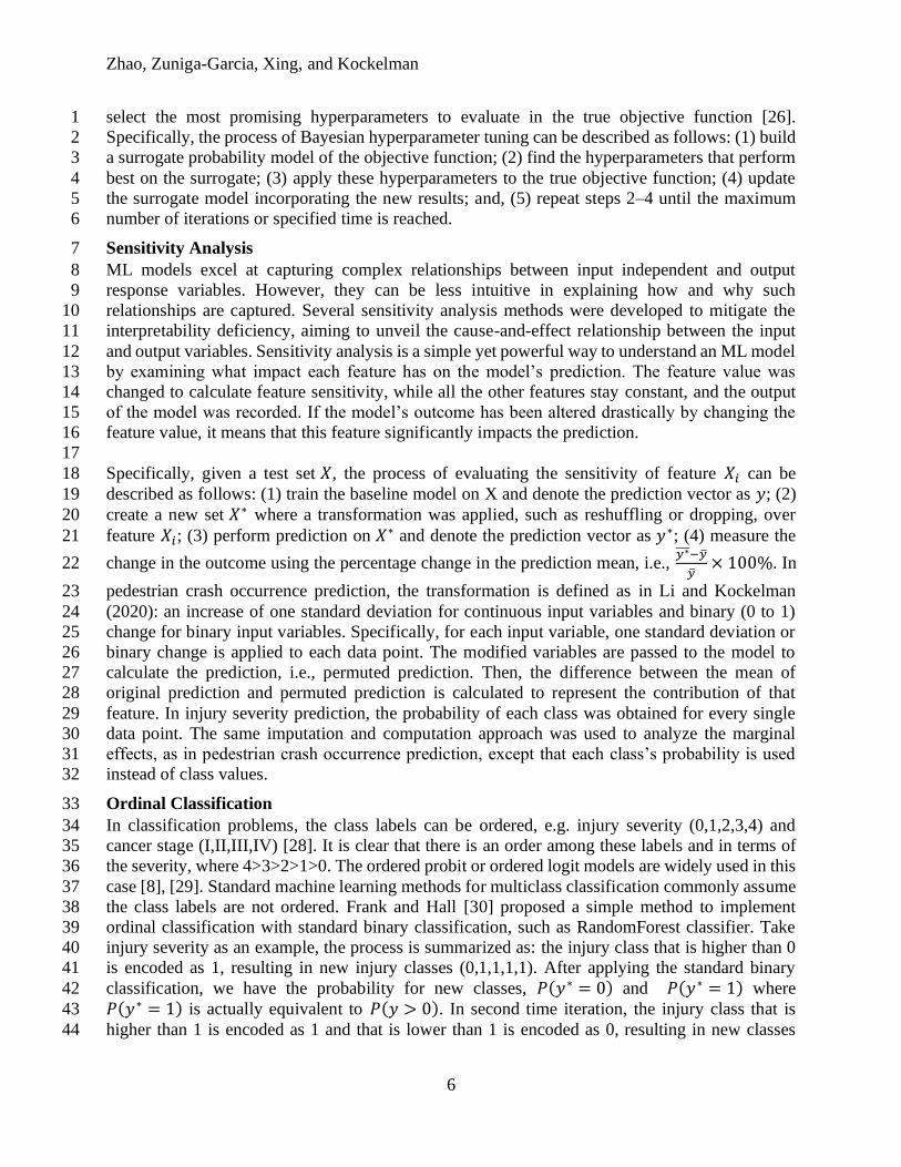
Feature Sensitivity Analysis 25
The practical importance of input variables can be estimated using the proposed sensitivity analysis 26
approach. The value of continuous features is increased by one standard deviation, and binary 27
changes are made on binary features for each data point in the dataset. Then the percentage change 28
in the mean of the model prediction is estimated. The estimated feature importance for total and 29
fatal pedestrian crash occurrence are shown in Figure 2. The y-axis shows the name of the input 30
variables. The x-axis represents the percentage change in the mean of model prediction, i.e., total 31
or fatal pedestrian crash occurrence, after applying the proposed transformation on the 32
corresponding input features. Different colors represent different ML models: blue for RF, orange 33
for LightGBM, green for XGBoost, and red for XBART. 34
35

Zhao, Zuniga-Garcia, Xing, and Kockelman
8
As shown in Figure 2, the vehicle miles traveled (VMT) have the most significant impact on total 1
and fatal pedestrian crash occurrence. One standard deviation increase on VMT can lead to around 2
a 270% and more than 300% increase in the total number and number of fatal pedestrian crash 3
occurrences per roadway segment, respectively. However, it should be noted that one standard 4
deviation increase of VMT (7,319) on all roadway segments is not practical, considering the 5
capacity limit of segments. Therefore, the process was repeated considering a double VMT on 6
each segment. The results indicate that the total and fatal pedestrian occurrence will increase by 7
50%, which is still a significant impact. These results, consistent with literature findings [31], 8
represent the higher crash risk faced by pedestrians with increasing VMT, which is consistent with 9
the expectation that crash frequencies increase with the increase in pedestrian exposure to 10
motorized vehicles. 11
12
The number of transit stops within a buffer of 100 meters is a relevant variable in predicting total 13
and fatal pedestrian crashes in roadway segments, according to the results of the LightGBM and 14
XBART models. This variable is an indirect measure of pedestrian exposure as pedestrian activity 15
surrounding transit stops is high. Similarly, variables for the distance to nearest school and distance 16
to nearest hospital offer a practical significance. The number of pedestrian crashes increases in 17
areas near schools and decreases as distance from schools increases, consistent with literature 18
findings [32]. Interestingly, the hospital proximity is particularly significant for fatal crashes, 19
where the frequency increases as the distance to the hospital increases, possibly related to the 20
response time of emergency services. Although relevant, these variables are rarely considered in 21
pedestrian safety literature [8]. 22
23
Highway design variables such as on-system roads (or state-maintained arterials), number of lanes, 24
curve angle, curvature indicator, and curvature length have a significant positive impact on 25
pedestrian crash frequencies. One standard deviation increment on the number of lanes can lead to 26
more than a 25% increment in total or fatal crash counts. On-system roads are found to be strongly 27
correlated to the number of total crashes. The speed limit is found to be negatively correlated to 28
the number of crashes. This can be related to the reduced exposure of pedestrians to high-speed 29
roadway segments. However, high speed limits lead to more severe injuries, as discussed in the 30
following section. Variables such as median and shoulder widths show diverse variations across 31
the different models, limiting the conclusions for these variables. 32
33
Land use characteristics are described by variables such as population, job density, and types of 34
urban areas. These metrics are directly related to pedestrian exposure. For example, dense urban 35
areas with high job density usually have higher traffic volumes and pedestrian activity. Changes 36
in one standard deviation led to a positive, significant increment in pedestrian crash frequencies, 37
as expected. The number of pedestrian crash occurrences increases by approximately 50% for total 38
counts and 30% for fatal counts when the population and job density are increased by one standard 39
deviation. Large-urbanized, urbanized, and small urban locations have more conservative 40
increments of 10% for total pedestrian crashes. However, for the fatal count model, the effect 41
differs significantly across models, possibly related to the low count number within the different 42
categories. 43
44
The four different models come to a similar conclusion about the significance of some features, 45
such as distance to the nearest school, job density, population density, and VMT. However, the 46

Zhao, Zuniga-Garcia, Xing, and Kockelman
9
results diverge on other features, such as the number of transit stops within a 100-meter buffer. 1
XBART and LightGBM consider the number of transit stops a very important feature in predicting 2
the total pedestrian crash occurrence. One standard deviation increase on the transit stop variable 3
can lead to 150% and 300% increase on total pedestrian crash occurrence, respectively. However, 4
results from LightGBM and XGBoost show that the number of transit stops has little impact on 5
the total pedestrian crash occurrence. This observation indicates that different ML models interpret 6
the significance of the input features differently. It might make more sense to look only at the 7
model that yields the best performance, i.e., prediction accuracy. Noticeably, the discrepancies in 8
the results from different models are even more obvious in fatal pedestrian occurrence prediction 9
as compared with total pedestrian occurrence. This again stresses the importance of choosing the 10
best performing model when comparing the evaluation metrics and then analyzing the feature 11
importance using the chosen optimal model. 12
Pedestrian Crash Injury Severity Prediction 13
To estimate the crash injury severity models, first, the complete dataset was randomly split into 14
training and testing datasets to predict crash injury severity. Then, four models (RF, XGBoost, 15
LightGBM, and XBART) were fitted on the training dataset and tested on the testing dataset. 16
Before model fitting, parameters for each model were tuned with the Bayesian optimization 17
method to obtain optimal parameters. The simulation was repeated ten times. 18
19
Model Performance Evaluation 20
Table 3 summarizes model performance on model running time, accuracy, precision, recall, F1 21
score, and GM. In general, RF, XGBoost, and LightGBM behave similarly in terms of these 22
classification metrics, but LightGBM runs much faster than the other two GBT models. Even with 23
higher precision, XBART shows lower recall and F1, and it is heavily time-consuming. The crash 24
injury data is imbalanced with 7%, 33%, 36%, 17%, and 7% of class 0 (not injured), 1 (possibly 25
injury), 2 (non-incapacitating), 3 (incapacitating) and 4 (killed), respectively. The geometric mean 26
(GM) metric is less sensitive to an imbalanced dataset [33]. Results show that RF, XGBoost, and 27
LightGBM achieve the same GM value of 0.53, which is higher than XBART with 0.51. This 28
indicates that XBART may be more sensitive to imbalanced data. 29
30
TABLE 3: Summary of model performance on injury severity prediction 31
Models Time (s) Accuracy Precision Recall F1 score GM
RandomForest 36.55 0.42 0.49 0.33 0.34 0.53
XGBoost 75.17 0.42 0.43 0.33 0.34 0.53
LightGBM 18.59 0.42 0.45 0.34 0.34 0.53
XBART 1447.56 0.42 0.53 0.31 0.32 0.51
32
Zhao, Zuniga-Garcia, Xing, and Kockelman
10
(a) Total pedestrian crash occurrence prediction
(b) Fatal pedestrian crash count prediction
FIGURE 2: Sensitivity analysis for crash occurrence predictions 1
2

Zhao, Zuniga-Garcia, Xing, and Kockelman
11
The model margins show the confidence of a classifier making a correct classification. A positive 1
margin value means the classifier votes for the right classification [20], and a negative margin 2
value indicates the classifier voted incorrectly. Figure 12 shows ten-time repeated results plotted 3
in a bar graph; model margins are affected by the injury class. For example, all four models achieve 4
higher margins on class 2 and class 4 (around 0.2), while the margin values for class 0 and class 3 5
are negative (-0.4 and -0.6), indicating a high discrepancy between true class and predicted class. 6
This discrepancy is not necessarily related to data imbalance as class 3 makes up a greater 7
proportion of the data than class 4, which has a higher margin. Also, XBART shows a much greater 8
capacity for correctly classifying class 2, while for other classes XBART is limited to a weak 9
classification capacity. 10
11
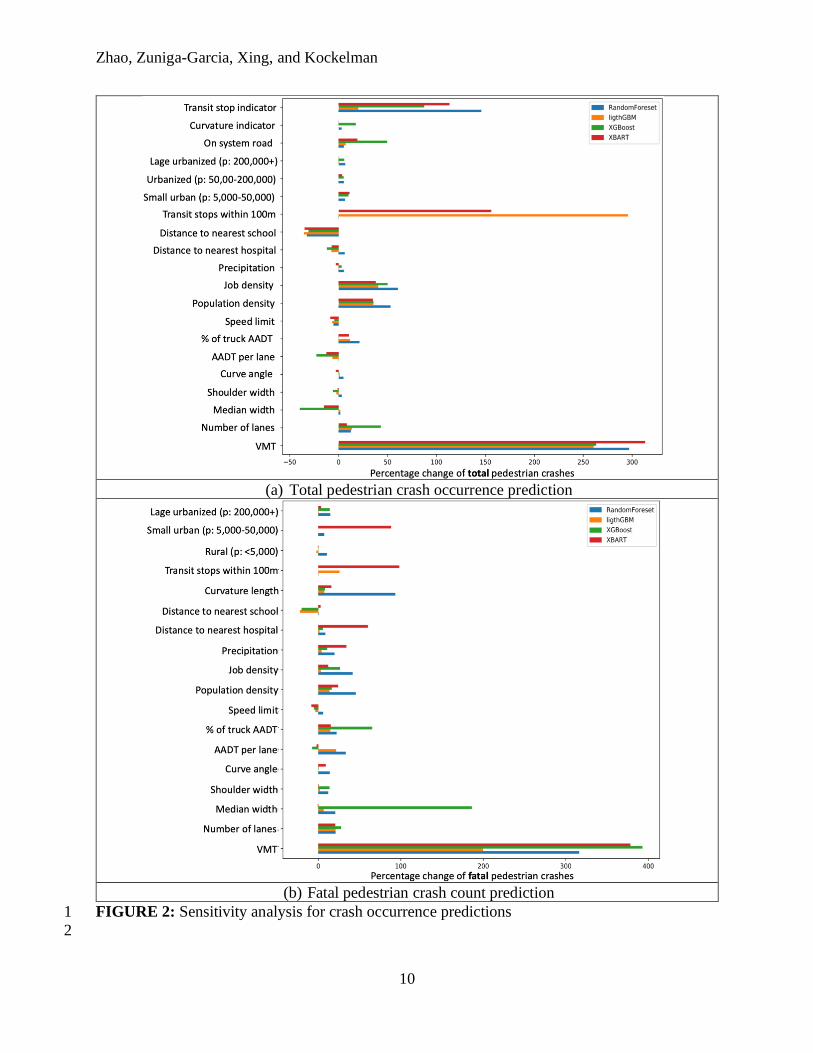
The ROC curve is one of the most important metrics to visualize the performance of multiclass 12
classification models. It quantifies the extent to which the model is able to distinguish between 13
classes (Narkhede, 2018). The AUC is the quantitative measure of ROC. The point (0,1) in the 14
ROC curve represents the prefect classifier, meaning no false-positive error happens (Fawcett, 15
2006). The ROC curve of one simulated result is presented in Figure 4 to analyze how those models 16
behave in the different classes. Based on the results, RF, XGBoost, and LightGBM are capable of 17
classifying on class 4 while achieving an AUC around 0.9. However, XBART shows less ability 18
to vote for the right classification on class 4 (AUC = 0.72). For other injury classes, RF, XGBoost, 19
and LightGBM obtain an AUC value ranging from 0.59 to 0.67, which exceeds that of XBART. 20
21
22 FIGURE 3: Margins of classification models on different classes 23
Zhao, Zuniga-Garcia, Xing, and Kockelman
12
a) RandomForest b) XGBoost
c) LightGBM d) XBART
FIGURE 4: ROC curve of different classification models 1
2
Marginal Effects 3
The marginal effects of each variable are analyzed by data imputation to identify the most 4
important factors that contribute to fatal pedestrian injury. First, the data is randomly split for 5
training and testing data. Then, the hyperparameters are optimized on the training data, and models 6
are trained on training data with optimal hyperparameters. Finally, the model is used for prediction 7
on the testing dataset before and after one variable is imputed, and the probability difference 8
between two times of prediction is defined as the marginal effect for that imputed variable. This 9
process is repeated ten times, and the results are summarized in Figure 5. 10
11
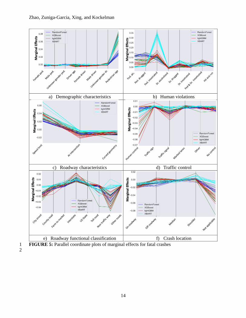
The variables are classified into ten categories. In terms of driver and pedestrian characteristics, 12
driver age seems to have both positive and negative marginal effects. This can be related to the 13
impact of driver age observed in some literature, with the involvement of younger drivers 14
increasing the risk of high severity as compared to the presence of middle-age drivers [34], [35]. 15
One study found that drivers aged 65 and older also increase the risk for pedestrian injury severity 16
[36]. However, some researchers have found that this is not always the case, as older drivers may 17
also be more experienced [37]. Furthermore, a high value for pedestrian age has a high likelihood 18
of increasing injury severity, which might be due to the greater physical vulnerability of older 19
people. 20
21

Zhao, Zuniga-Garcia, Xing, and Kockelman
13
Several human violation variables were tested to analyze the effect of pedestrian and driver 1
intoxication. Figure 5b shows that the intoxicated pedestrian variable is the most important factor 2
that contributes to fatal pedestrian injury among those variables. The probability of a pedestrian 3
fatality shows significant positive changes after data imputation, indicating that pedestrian 4
intoxication greatly increases the risks of pedestrian death in a crash. When pedestrian intoxication 5
is imputed, the probability of pedestrian death increases by 15% on average in RF, XGBoost, and 6
LightGBM models, and XBART shows a probability change as great as 30%. Driver intoxication 7
also leads to an increase in pedestrian death probability change. Intoxication is more likely to cause 8
pedestrian fatality in a crash, and this result is also supported by the CRIS dataset, where 9
intoxication is involved in 38% of fatal crashes. The simulation result is consistent with the 10
previous report that intoxication has the strongest effect on pedestrian death [8]. Hit-and-run 11
accidents are also related to a high pedestrian severity level. In the CRIS data, 19% of pedestrian 12
deaths are hit-and-run cases, highlighting the relevance of this variable. The high severity is largely 13
due to the time delay incurred when the driver leaves the crash location, which delays emergency 14
services and prompt attention to the pedestrian. 15
16
Speed limit contributes significantly to the probability of pedestrian death, and the marginal effect 17
ranges from 2% to 6% among these classification models. As expected, roads with higher speed 18
limits led to more pedestrian injuries, consistent with previous studies [38]. However, crash 19
frequency is reduced as speed limit increases, as found in the analysis of the previous section. 20
Approximately 21% of the crashes were located at intersections. The results indicate that those 21
crashes have a lesser risk of pedestrian fatalities than mid-segment crashes, likely due to reduced 22
speed at these locations. Traffic control, including traffic signs and traffic signals, can help to 23
reduce the probability of a crash and thus pedestrian death. Results suggest that traffic control is 24
predicted to reduce pedestrian death probability on average by 3% in LightGBM, 2% in XGBoost, 25
1% in XBART, and 0.5% in RF. Also, data imputation on traffic signals decreases pedestrian death 26
probability by as much as 2% on average in LightGBM. 27
28
Roadway functional classification is also an important factor. Different road types (such as country 29
roads, city streets, and interstate roads) also play distinct roles in fatal pedestrian injury. For 30
example, city streets and non-trafficways help reduce the marginal effect in RF, XGBoost, and 31
LightGBM models, while the interstate seems to increase the marginal impact on all models. In 32
Texas, interstate highways account for 6% of pedestrian crashes but 21% of pedestrian fatalities. 33
This outcome is likely related to the speed of the crash. As analyzed previously, high-speed 34
roadway segments tend to have fewer pedestrian crashes, but the severity is higher due to the speed 35
of impact. The crash location analysis seems to indicate that crashes occurring on the roadway 36
shoulder have a higher risk of causing pedestrian fatalities compared to crashes on the roadway 37
and in the median area. 38
39
The area type is also an important factor for injury severity. The results suggest that rural and small 40
urban areas present a higher risk for pedestrian fatalities. Factors such as distance to hospitals and 41
speed limits can influence this finding. Rural and small urban areas tend to be less dense, and the 42
emergency response time is slower than in urban areas. However, results from the previous section 43
indicate that pedestrian activity is lower in these areas compared to large urban areas. 44
45
Zhao, Zuniga-Garcia, Xing, and Kockelman
14
a) Demographic characteristics b) Human violations
c) Roadway characteristics d) Traffic control
e) Roadway functional classification f) Crash location
FIGURE 5: Parallel coordinate plots of marginal effects for fatal crashes 1
2

Zhao, Zuniga-Garcia, Xing, and Kockelman
15
g) Area type h) Vehicle type
i) Time of the day j) Lighting conditions
FIGURE 5: Parallel coordinate plots of marginal effects for fatal crashes (Cont.) 1
2
In terms of vehicle types, research in the field indicates that high injury severity is associated with 3
light-duty vehicles, such as SUV/CUVs, pickup trucks, and vans, due to the heavy mass involved 4
in the collision [8], [35], [39], [40]. However, this study shows that trucks involved in a crash are 5
more likely to cause the death of pedestrians, but the effects of vans and SUV/CUVs are not 6
significant. Busses also have a significant effect, but it is important to mention that the number of 7
crashes involving buses is low compared to other vehicle body types. 8
9
Environmental factors such as crash time and lighting condition strongly affect the pedestrian 10
injury severity [35], [41]. The time of day is found to influence its marginal effect. Specifically, 11
the period after 8 PM and before 7 AM (under dark conditions) has a positive effect on pedestrian 12
deaths. Approximately 80% of pedestrian deaths occurred at this time. In contrast, in the daytime, 13
the probability of pedestrian death is reduced in all models. Similarly, the brighter daytime 14
conditions significantly help to lower the likelihood of pedestrian death in all models, but not the 15
other light types. This finding highlights the importance of streetlight improvements to reduce 16
pedestrian crashes. 17
CONCLUSIONS 18
Tree-based machine learning models were applied to identify major factors contributing to 19
pedestrian-vehicle crash occurrences and pedestrian injury severity. The analysis showed that 20
Zhao, Zuniga-Garcia, Xing, and Kockelman
16
pedestrian and driver intoxication levels, speed limit, and lighting conditions significantly affect 1
the severity of crashes. Variables such as crash location, traffic control, and roadway 2
characteristics were also analyzed. The principal findings suggest that crashes located at 3
intersections have a lesser risk of pedestrian fatalities than mid-segment crashes, likely due to 4
reduced speeds at these locations. Also, traffic control, including traffic signs and traffic signals, 5
can help to reduce the probability of a crash and pedestrian death. In terms of pedestrian crash 6
frequencies, VMT was one of the most significant variables, and the number of transit stops within 7
a buffer of 100 meters was relevant in predicting total and fatal pedestrian crashes in roadway 8
segments. Results also found that highway design variables significantly positively impact 9
pedestrian crash frequencies. Finally, the number of pedestrian crash occurrences increases by 10
more than one third when the population and job density increase by one standard deviation. 11
12
This study also showed a comparison across four different tree-based models. In the pedestrian 13
crash occurrence prediction, the principal results showed that all four models perform similarly, 14
with close root mean square error (RMSE) and R-square for total crash occurrence. Still, 15
LightGBM exceeds the other three models in terms of computational efficiency. For fatal crash 16
occurrence, LightGBM and RF have comparable performance. However, XGBoost and XBART 17
showed significantly lower goodness of fit values. Also, XBART is more sensitive to imbalanced 18
data than the other models are. In the injury severity prediction, RF, XGBoost, and LightGBM 19
achieved similar goodness of fit performance, evaluated by the metrics’ accuracy, precision, recall, 20
F1, and geometric mean. XBART obtained a higher precision value, but the other metrics were 21
lower, with a significantly high computational time. 22
23
Findings from this study underscore the importance of campaigns against driving and walking 24
while intoxicated, installation of streetlights in pedestrian-active areas, improved roadway design, 25
and enforcement of safety countermeasures in areas where pedestrians are more vulnerable (such 26
as near bus stops and schools). It also highlights the importance of detailed police reports to 27
develop analyses of this type that can be used to improve pedestrian safety. 28
AUTHOR CONTRIBUTION STATEMENT 29
The authors confirm contribution to the paper as follows: writing-original draft preparation: B. 30
Zhao, N. Zuniga-Garcia, L. Xing; conceptualization and design: K. Kockelman, B. Zhao, L. Xing; 31
methodology: K. Kockelman, B. Zhao, L. Xing; data assembly and analysis: B. Zhao, L. Xing, N. 32
Zuniga-Garcia; writing-reviewing and editing: N. Zuniga-Garcia, B. Zhao, L. Xing, K. 33
Kockelman. All authors have reviewed the results and approved the final version of the 34
manuscript. 35
REFERENCES 36
[1] H. Christian et al., “Encouraging Dog Walking for Health Promotion and Disease Prevention,” 37
Am. J. Lifestyle Med., vol. 12, no. 3, pp. 233–243, May 2018, doi: 38
10.1177/1559827616643686. 39
[2] P. Kelly, M. Murphy, and N. Mutrie, “The Health Benefits of Walking,” in Walking, vol. 9, 40
Emerald Publishing Limited, 2017, pp. 61–79. doi: 10.1108/S2044-994120170000009004. 41
[3] G. H. S. A. GHSA, “Pedestrian Traffic Fatalities by State,” 2020. 42
[4] U. States. D. O. Transportation. B. O. T. S. BTS, “National Transportation Statistics: U.S. 43
Passenger-Miles,” 2019. 44

Zhao, Zuniga-Garcia, Xing, and Kockelman
17
https://rosap.ntl.bts.gov/gsearch?collection=dot:35533&type1=mods.title&fedora_terms1=1
National+Transportation+Statistics (accessed May 16, 2021). 2
[5] F. H. A. FHWA, “Summary of Travel Trends 2017 National Household Travel Survey,” 3
ORNL/TM-2004/297, 885762, 2018. doi: 10.2172/885762. 4
[6] R. Elvik, “The non-linearity of risk and the promotion of environmentally sustainable 5
transport,” Accid. Anal. Prev., vol. 41, no. 4, pp. 849–855, Jul. 2009, doi: 6
10.1016/j.aap.2009.04.009. 7
[7] C. Lee and M. Abdel-Aty, “Comprehensive analysis of vehicle–pedestrian crashes at 8
intersections in Florida,” Accid. Anal. Prev., vol. 37, no. 4, pp. 775–786, Jul. 2005, doi: 9
10.1016/j.aap.2005.03.019. 10
[8] Rahman, M. and Kockelman, K.M., 2020. Predicting Pedestrian Crash Occurrences and Injury 11
Severity in Texas Presented at the 100th Annual Meeting of the Transportation Research Board. 12
Under review for publication in Traffic Injury and Prevention. 13
[9] S. Ukkusuri, L. F. Miranda-Moreno, G. Ramadurai, and J. Isa-Tavarez, “The role of built 14
environment on pedestrian crash frequency,” Saf. Sci., vol. 50, no. 4, pp. 1141–1151, Apr. 15
2012, doi: 10.1016/j.ssci.2011.09.012. 16
[10] Y. Wang and K. M. Kockelman, “A Poisson-lognormal conditional-autoregressive model for 17
multivariate spatial analysis of pedestrian crash counts across neighborhoods,” Accid. Anal. 18
Prev., vol. 60, pp. 71–84, Nov. 2013, doi: 10.1016/j.aap.2013.07.030. 19
[11] L. Yue, M. Abdel-Aty, Y. Wu, O. Zheng, and J. Yuan, “In-depth approach for identifying 20
crash causation patterns and its implications for pedestrian crash prevention,” J. Safety Res., 21
vol. 73, pp. 119–132, Jun. 2020, doi: 10.1016/j.jsr.2020.02.020. 22
[12] M. Wier, J. Weintraub, E. H. Humphreys, E. Seto, and R. Bhatia, “An area-level model of 23
vehicle-pedestrian injury collisions with implications for land use and transportation 24
planning,” Accid. Anal. Prev., vol. 41, no. 1, pp. 137–145, Jan. 2009, doi: 25
10.1016/j.aap.2008.10.001. 26
[13] M. Vahedi Saheli and M. Effati, “Segment-Based Count Regression Geospatial Modeling of 27
the Effect of Roadside Land Uses on Pedestrian Crash Frequency in Rural Roads,” Int. J. 28
Intell. Transp. Syst. Res., vol. 19, no. 2, pp. 347–365, Jun. 2021, doi: 10.1007/s13177-020-29
00250-1. 30
[14] R. Tay, J. Choi, L. Kattan, and A. Khan, “A multinomial logit model of pedestrian–vehicle 31
crash severity,” Int. J. Sustain. Transp., vol. 5, no. 4, pp. 233–249, 2011. 32
[15] J.-K. Kim, G. F. Ulfarsson, V. N. Shankar, and S. Kim, “Age and pedestrian injury severity 33
in motor-vehicle crashes: A heteroskedastic logit analysis,” Accid. Anal. Prev., vol. 40, no. 34
5, pp. 1695–1702, Sep. 2008, doi: 10.1016/j.aap.2008.06.005. 35
[16] M. Effati and M. Vahedi Saheli, “Examining the influence of rural land uses and 36
accessibility-related factors to estimate pedestrian safety: The use of GIS and machine 37
learning techniques,” Int. J. Transp. Sci. Technol., Apr. 2021, doi: 38
10.1016/j.ijtst.2021.03.005. 39
[17] S. Mokhtarimousavi, J. C. Anderson, A. Azizinamini, and M. Hadi, “Factors affecting injury 40
severity in vehicle-pedestrian crashes: A day-of-week analysis using random parameter 41
ordered response models and Artificial Neural Networks,” Int. J. Transp. Sci. Technol., vol. 42
9, no. 2, pp. 100–115, Jun. 2020, doi: 10.1016/j.ijtst.2020.01.001. 43
[18] S. K. Sivasankaran and V. Balasubramanian, “Severity of Pedestrians in Pedestrian - Bus 44
Crashes: An Investigation of Pedestrian, Driver and Environmental Characteristics Using 45
Random Forest Approach,” in Proceedings of the 21st Congress of the International 46

Zhao, Zuniga-Garcia, Xing, and Kockelman
18
Ergonomics Association (IEA 2021), Cham, 2021, pp. 825–833. doi: 10.1007/978-3-030-1
74608-7_101. 2
[19] M. Guo, Z. Yuan, B. Janson, Y. Peng, Y. Yang, and W. Wang, “Older Pedestrian Traffic 3
Crashes Severity Analysis Based on an Emerging Machine Learning XGBoost,” 4
Sustainability, vol. 13, no. 2, Art. no. 2, Jan. 2021, doi: 10.3390/su13020926. 5
[20] L. Breiman, “Random forests,” Mach. Learn., vol. 45, no. 1, pp. 5–32, 2001, doi: 6
10.1023/A:1010933404324. 7
[21] A. Liaw and M. Wiener, “Classification and Regression by randomForest,” R News, vol. 2, 8
no. 3, pp. 18–22, 2002. 9
[22] T. Chen and C. Guestrin, “XGBoost: A scalable tree boosting system,” in Proceedings of the 10
ACM SIGKDD International Conference on Knowledge Discovery and Data Mining, 2016, 11
pp. 785--794. doi: 10.1145/2939672.2939785. 12
[23] G. Ke et al., “LightGBM: A highly efficient gradient boosting decision tree,” 2017. 13
[24] H. A. Chipman, E. I. George, and R. E. McCulloch, “BART: Bayesian additive regression 14
trees,” Ann. Appl. Stat., 2012, doi: 10.1214/09-AOAS285. 15
[25] J. He, S. Yalov, and P. R. Hahn, “XBART: Accelerated Bayesian additive regression trees,” 16
arXiv. 2018. 17
[26] A. Klein, S. Falkner, S. Bartels, P. Hennig, and F. Hutter, “Fast Bayesian optimization of 18
machine learning hyperparameters on large datasets,” in Artificial Intelligence and Statistics, 19
2017, pp. 528--536. 20
[27] W. Li and K. M. Kockelman, “How does machine learning compare to conventional 21
econometrics for transport data sets? A test of ML vs MLE,” Transp. Res. Rec., 2020. 22
[28] B. Misganaw and M. Vidyasagar, “Exploiting Ordinal Class Structure in Multiclass 23
Classification: Application to Ovarian Cancer,” IEEE Life Sci. Lett., 2015, doi: 24
10.1109/LLS.2015.2451291. 25
[29] X. Wang and K. M. Kockelman, “Occupant injury severity using a heteroscedastic ordered 26
logit model: distinguishing the effects of vehicle weight and type,” Transp. Res. Rec., vol. 27
1908, pp. 195–204, 2005. 28
[30] E. Frank and M. Hall, “A simple approach to ordinal classification,” in European Conference 29
on Machine Learning, 2001, pp. 145--156. doi: 10.1007/3-540-44795-4_13. 30
[31] T. Nashad, S. Yasmin, N. Eluru, J. Lee, and M. A. Abdel-Aty, “Joint Modeling of Pedestrian 31
and Bicycle Crashes: Copula-Based Approach,” Transp. Res. Rec., vol. 2601, no. 1, pp. 119–32
127, Jan. 2016, doi: 10.3141/2601-14. 33
[32] J. Warsh, L. Rothman, M. Slater, C. Steverango, and A. Howard, “Are school zones 34
effective? An examination of motor vehicle versus child pedestrian crashes near schools,” 35
Inj. Prev. J. Int. Soc. Child Adolesc. Inj. Prev., vol. 15, no. 4, pp. 226–229, Aug. 2009, doi: 36
10.1136/ip.2008.020446. 37
[33] A. Tharwat, “Classification assessment methods,” Appl. Comput. Inform., 2018, doi: 38
10.1016/j.aci.2018.08.003. 39
[34] J.-K. Kim, G. F. Ulfarsson, V. N. Shankar, and F. L. Mannering, “A note on modeling 40
pedestrian-injury severity in motor-vehicle crashes with the mixed logit model,” Accid. Anal. 41
Prev., vol. 42, no. 6, pp. 1751–1758, Nov. 2010, doi: 10.1016/j.aap.2010.04.016. 42
[35] M. Pour-Rouholamin and H. Zhou, “Investigating the risk factors associated with pedestrian 43
injury severity in Illinois,” J. Safety Res., vol. 57, pp. 9–17, Jun. 2016, doi: 44
10.1016/j.jsr.2016.03.004. 45
Zhao, Zuniga-Garcia, Xing, and Kockelman
19
[36] M. G. Mohamed, N. Saunier, L. F. Miranda-Moreno, and S. V. Ukkusuri, “A clustering 1
regression approach: A comprehensive injury severity analysis of pedestrian–vehicle crashes 2
in New York, US and Montreal, Canada,” Saf. Sci., vol. 54, pp. 27–37, Apr. 2013, doi: 3
10.1016/j.ssci.2012.11.001. 4
[37] J. M. Wood, P. Lacherez, and R. A. Tyrrell, “Seeing pedestrians at night: effect of driver age 5
and visual abilities,” Ophthalmic Physiol. Opt., vol. 34, no. 4, pp. 452–458, 2014. 6
[38] Z. Chen and W. (David) Fan, “A multinomial logit model of pedestrian-vehicle crash severity 7
in North Carolina,” Int. J. Transp. Sci. Technol., vol. 8, no. 1, pp. 43–52, Mar. 2019, doi: 8
10.1016/j.ijtst.2018.10.001. 9
[39] A. J. Anarkooli, M. Hosseinpour, and A. Kardar, “Investigation of factors affecting the injury 10
severity of single-vehicle rollover crashes: A random-effects generalized ordered probit 11
model,” Accid. Anal. Prev., vol. 106, pp. 399–410, Sep. 2017, doi: 12
10.1016/j.aap.2017.07.008. 13
[40] J. Liu, A. Hainen, X. Li, Q. Nie, and S. Nambisan, “Pedestrian injury severity in motor 14
vehicle crashes: An integrated spatio-temporal modeling approach,” Accid. Anal. Prev., vol. 15
132, p. 105272, Nov. 2019, doi: 10.1016/j.aap.2019.105272. 16
[41] H. M. A. Aziz, S. V. Ukkusuri, and S. Hasan, “Exploring the determinants of pedestrian–17
vehicle crash severity in New York City,” Accid. Anal. Prev., vol. 50, pp. 1298–1309, Jan. 18
2013, doi: 10.1016/j.aap.2012.09.034. 19
20